Conformal Prediction Beyond Exchangeability

Abstract

Conformal prediction is a popular, modern technique for providing valid predictive inference for arbitrary machine learning models. Its validity relies on the assumptions of exchangeability of the data, and symmetry of the given model fitting algorithm as a function of the data. However, exchangeability is often violated when predictive models are deployed in practice. For example, if the data distribution drifts over time, then the data points are no longer exchangeable; moreover, in such settings, we might want to use a nonsymmetric algorithm that treats recent observations as more relevant. This paper generalizes conformal prediction to deal with both aspects: we employ weighted quantiles to introduce robustness against distribution drift, and design a new randomization technique to allow for algorithms that do not treat data points symmetrically. Our new methods are provably robust, with substantially less loss of coverage when exchangeability is violated due to distribution drift or other challenging features of real data, while also achieving the same coverage guarantees as existing conformal prediction methods if the data points are in fact exchangeable. We demonstrate the practical utility of these new tools with simulations and real-data experiments on electricity and election forecasting.

1 Introduction

The field of conformal prediction addresses a challenging modern problem: given a “black box” algorithm that fits a predictive model to available training data, how can we calibrate prediction intervals around the output of the model so that these intervals are guaranteed to achieve some desired coverage level?

As an example, consider a holdout set approach. Suppose we have a pre-fitted model $\widehat{\mu}$ mapping features $X$ to a prediction of a real-valued variable $Y$ (e.g., $\widehat{\mu}$ is the output of some machine learning algorithm trained on a prior data set), and a fresh holdout set of data $(X_{1},Y_{1}),\dots,(X_{n},Y_{n})$ not used for training. We can then use the empirical quantiles of the errors $|Y_{i}-\widehat{\mu}(X_{i})|$ on the holdout set to compute a prediction interval around our prediction $\widehat{\mu}(X_{n+1})$ that aims to cover the unseen response $Y_{n+1}$. Split conformal prediction (Vovk et al., 2005) formalizes this method, and gives guaranteed predictive coverage when the data points $(X_{i},Y_{i})$ are drawn i.i.d. from any distribution (see Section 2). However, the validity of this method hinges on the assumption that the data points are drawn independently from the same distribution, or more generally, that $(X_{1},Y_{1}),\dots,(X_{n+1},Y_{n+1})$ are exchangeable.

In many applied domains, this assumption is often substantially violated, due to distribution drift, correlations between data points, or other phenomena. As an example, Figure 1 shows results from an experiment on a real data set monitoring electricity usage in Australia (the ELEC2 data set (Harries, 1999), which we return to in Section 5.2). We see that over a substantial stretch of time, conformal prediction loses coverage, its intervals decreasing far below the target 90% coverage level, while our proposed method, nonexchangeable conformal prediction, is able to maintain approximately the desired coverage level. In this paper, we will see how to quantify the loss of coverage due to violations of exchangeability, and how we can modify the conformal prediction methodology to regain predictive coverage even in the presence of distribution drift or other violations of exchangeability.

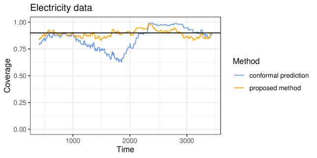
Figure 1: Empirical results from a real data set (details will be given in Section 5.2).

1.1 Beyond exchangeability

In this paper, we will consider three important classes of methods for distribution-free prediction: split conformal, full conformal, and the jackknife+. (We give background on split and full conformal in Section 2, and on jackknife+ in Appendix B.) These methods rely on exchangeability in two different ways:

• The data $Z_{i}=(X_{i},Y_{i})$ are assumed to be exchangeable (for example, i.i.d.).

• The algorithm $\mathcal{A}$, which maps data to a fitted model $\widehat{\mu}:\mathcal{X}\rightarrow\mathbb{R}$, is assumed to treat the data points symmetrically, to ensure that exchangeability of the data points $Z_{i}$ still holds even after we observe the fitted model(s).

In this work, we aim to provide distribution-free prediction guarantees when we drop both of these assumptions:

• We may have data points $Z_{i}$ that are not exchangeable—for instance, they may be independent but nonidentically distributed (e.g., due to distribution drift), or there may be dependence among them that creates nonexchangeability (e.g., correlation over space or time).

• We may wish to use an algorithm $\mathcal{A}$ that does not treat the input data points symmetrically—for example, if $Z_{i}$ denotes data collected at time $i$, we may prefer to fit a model $\widehat{\mu}$ that places higher weight on more recent data points.

1.2 Our contributions

We generalize the split conformal, full conformal, and jackknife+ methods (detailed later) to allow for both of these sources of nonexchangeability. Our procedures can recover the original variants if a symmetric algorithm is employed. We will provide coverage guarantees that are identical to existing guarantees if the data points are in fact exchangeable, and only slightly lower if the deviation from exchangeability is mild.

To elaborate, let us define the coverage gap as the loss in coverage compared to what is achieved under exchangeability. For example, in split conformal prediction run with a desired coverage level $1-\alpha$, we have

$$\textnormal{Coverage gap}=(1-\alpha)-\mathbb{P}\left\{{Y_{n+1}\in\widehat{C}_{n}(X_{n+1})}\right\},$$

since, under exchangeability, the method guarantees coverage with probability $1-\alpha$. To give an informal preview of our results, we write $Z_{i}=(X_{i},Y_{i})$ to denote the $i$th data point and

$$Z=(Z_{1},\dots,Z_{n+1})$$ (1)

to denote the full (training and test) data sequence, and let $Z^{i}$ denote this sequence after swapping the test point $(X_{n+1},Y_{n+1})$ with the $i$th training point $(X_{i},Y_{i})$:

$$Z^{i}=(Z_{1},\dots,Z_{i-1},Z_{n+1},Z_{i+1},\dots,Z_{n},Z_{i}).$$ (2)

To enable robustness, our methods will allow for weights: let $w_{i}\in[0,1]$ denote a prespecified weight placed on data point $i$. We will see that the coverage gap can be bounded as

$$\textnormal{Coverage gap}\leq\frac{\sum_{i=1}^{n}w_{i}\cdot\mathsf{d}_{\mathsf{TV}}(Z,Z^{i})}{1+\sum_{i=1}^{n}w_{i}},$$ (3)

where $\mathsf{d}_{\mathsf{TV}}$ denotes the total variation distance between distributions. Notably, we do not make any assumption on the joint distribution of the $n+1$ points. Of course, the result will only be meaningful if we are able to select fixed (non-data-dependent) weights $w_{i}$ such that this upper bound is likely to be small. In particular, if we use these methods, we are implicitly assuming that this weighted sum of total variation terms is small. In contrast, past work on conformal prediction in a model-free setting has relied on the assumption that the data are exactly exchangeable, since no prior results offered an analysis of the coverage gap under violations of exchangeability. See Section 4.3 for further discussion.

Note that the upper bound in (3) is a far stronger result than simply asking whether the data is “nearly exchangeable”. For instance, in a time series, it might be the case that $\mathsf{d}_{\mathsf{TV}}(Z,Z^{i})$ is quite small but $\mathsf{d}_{\mathsf{TV}}(Z,Z_{\pi})\approx 1$ for most permutations $\pi$. In words, if the observations are noisy, then permuting only two data points might not be detectable—but if there is nonstationarity or dependence over time then $Z$ is likely to be far from exchangeable.

Several further remarks are in order. First, for $w_{i}\equiv 1$ and a symmetric algorithm, the proposed weighted methods will reduce to the usual conformal (or jackknife+) methods. Thus, the result (3) also quantifies the degradation in coverage of standard methods in nonexchangeable settings. Second, this result has new implications in exchangeable settings: if the data points are in fact exchangeable (with i.i.d. as a special case), then $Z\stackrel{{\scriptstyle\textnormal{d}}}{{=}}Z^{i}$ and the coverage gap bound in (3) is equal to zero (here we use $\stackrel{{\scriptstyle\textnormal{d}}}{{=}}$ for equality in distribution). Therefore, our use of a weighted conformal procedure (rather than choosing $w_{i}\equiv 1$, which is the original unweighted procedure) does not hurt coverage if the data are exchangeable. Finally, the result provides insights on why one might prefer to use our new weighted procedures in (possibly) nonexchangeable settings: it can provide robustness in the case of distribution shift. To elaborate, consider a setting where the data points $Z_{i}$ are independent, but are not identically distributed due to distribution drift. The following result relates $\mathsf{d}_{\mathsf{TV}}(Z,Z^{i})$ to the distributions of the individual data points.

Lemma 1.

If $Z_{1},\dots,Z_{n+1}$ are independent, then

$$\mathsf{d}_{\mathsf{TV}}(Z,Z^{i})\leq 2\mathsf{d}_{\mathsf{TV}}(Z_{i},Z_{n+1})-\mathsf{d}_{\mathsf{TV}}(Z_{i},Z_{n+1})^{2}\leq 2\mathsf{d}_{\mathsf{TV}}(Z_{i},Z_{n+1}).$$

Combining this lemma with (3), we can see that if we are able to place small weights $w_{i}$ on data points $Z_{i}$ with large total variation distance $\mathsf{d}_{\mathsf{TV}}(Z_{i},Z_{n+1})$, then the coverage gap will be low. For example, under distribution drift, we might have $\mathsf{d}_{\mathsf{TV}}(Z_{i},Z_{n+1})$ decreasing with $i$; we can achieve a low coverage gap by using, say, weights $w_{i}=\rho^{n+1-i}$ for some $\rho<1$. We will return to this example in Section 4.4.

We will also see that the result in (3) actually stems from a stronger result:

$$\textnormal{Coverage gap}\leq\frac{\sum_{i=1}^{n}w_{i}\cdot\mathsf{d}_{\mathsf{TV}}(R(Z),R(Z^{i}))}{1+\sum_{i=1}^{n}w_{i}}.$$ (4)

Here $R(Z)$ denotes a vector of residuals: for split conformal prediction, this is the vector with entries $R(Z)_{i}=|Y_{i}-\widehat{\mu}(X_{i})|$, where $\widehat{\mu}$ is a pre-fitted model, while for full conformal the entries are again given by $R(Z)_{i}=|Y_{i}-\widehat{\mu}(X_{i})|$ but now $\widehat{\mu}$ is the model obtained by running $\mathcal{A}$ on the entire data sequence $Z$. Now $R(Z^{i})$ is simply the same function applied to the swapped data $Z^{i}$ instead of $Z$—that is, the residuals are computed after swapping data points $i$ and $n+1$ in the data set. (We also later generalize to any outcome space $\mathcal{Y}$ and to other definitions of residuals.)

Clearly, the bound in (4) is strictly stronger than (3), because the total variation distance between any function applied to each of $Z$ and $Z^{i}$, cannot be larger than $\mathsf{d}_{\mathsf{TV}}(Z,Z^{i})$ itself—and in many cases, the bound in (4) may be substantially tighter. For example, if the data is high dimensional, with $Z_{i}=(X_{i},Y_{i})\in\mathbb{R}^{p}\times\mathbb{R}$ for large $p$, then the distance $\mathsf{d}_{\mathsf{TV}}(Z,Z^{i})$ may be extremely large since $Z$ and $Z^{i}$ each contain $p+1$ dimensions of information about each data point. On the other hand, if we only observe the residuals (e.g., $R(Z)_{i}=|Y_{i}-\widehat{\mu}(X_{i})|$ for each $i$), then this reveals only a one-dimensional summary of each data point; this typically reduces the distance between the two distributions, and by a considerable amount if the distribution drift occurs in features that happen to be irrelevant for prediction and are thus ignored by $\widehat{\mu}$. In Section 4.4, we will see a specific example demonstrating the potentially large gap between these two upper bounds.

2 Background and related work

We briefly review several distribution-free prediction methods that offer guarantees under an exchangeability assumption on the data and symmetry of the underlying algorithm. We also set up notation that will be useful later in the paper.

Split conformal prediction.

Split conformal prediction (Vovk et al., 2005) (also called inductive conformal prediction) is a holdout method for constructing prediction intervals around a pre-trained model. Specifically, given a model $\widehat{\mu}:\mathcal{X}\rightarrow\mathbb{R}$ that was fitted on an initial training data set, and given $n$ additional data points $(X_{1},Y_{1}),\dots,(X_{n},Y_{n})$ (the holdout set), we define residuals

$$R_{i}=|Y_{i}-\widehat{\mu}(X_{i})|,\ i=1,\dots,n,$$

and then compute the prediction interval at the new feature vector $X_{n+1}$ as

$$\widehat{C}_{n}(X_{n+1})=\widehat{\mu}(X_{n+1})\pm\textnormal{(the $\lceil(1-\alpha)(n+1)\rceil$-th smallest of $R_{1},\dots,R_{n}$)}.$$

Equivalently, we can write

$$\widehat{C}_{n}(X_{n+1})=\widehat{\mu}(X_{n+1})\pm\mathsf{Q}_{1-\alpha}\left(\sum_{i=1}^{n}\tfrac{1}{n+1}\cdot\delta_{R_{i}}+\tfrac{1}{n+1}\cdot\delta_{+\infty}\right),$$ (5)

where $\mathsf{Q}_{\tau}(\cdot)$ denotes the $\tau$-quantile of its argument, and $\delta_{a}$ denotes the point mass at $a$. This method is well-known to guarantee distribution-free predictive coverage at the target level $1-\alpha$.

A drawback of the split conformal method is the loss of accuracy due to sample splitting, since the pre-trained model $\widehat{\mu}$ needs to be independent from the holdout set—in practice, if only $n$ labeled data points are available in total, we might use $n/2$ data points for training $\widehat{\mu}$, and then the procedure defined in (5) above would actually be run with a holdout set of size $n/2$ in place of $n$. In this paper, however, we will continue to write $n$ to denote the holdout set size for the split conformal method, in order to allow for universal notation across different methods.

Full conformal prediction.

To avoid the cost of data splitting, an alternative is the full conformal method (Vovk et al., 2005), also referred to as transductive conformal prediction. Fix any regression algorithm

$$\mathcal{A}:\ \cup_{n\geq 0}\left(\mathcal{X}\times\mathbb{R}\right)^{n}\ \rightarrow\ \left\{\textnormal{measurable functions $\widehat{\mu}:\mathcal{X}\rightarrow\mathbb{R}$}\right\},$$

which maps a data set containing any number of pairs $(X_{i},Y_{i})$, to a fitted regression function $\widehat{\mu}$. The algorithm $\mathcal{A}$ is required to treat data points symmetrically, i.e.,

$$\mathcal{A}\big{(}(x_{\pi(1)},y_{\pi(1)}),\dots,(x_{\pi(n)},y_{\pi(n)})\big{)}=\mathcal{A}\big{(}(x_{1},y_{1}),\dots,(x_{n},y_{n})\big{)}$$ (6)

for all $n\geq 1$, all permutations $\pi$ on $[n]:=\{1,\dots,n\}$, and all $\{(x_{i},y_{i})\}_{i=1,\dots,n}$. Next, for each $y\in\mathbb{R}$, let

$$\widehat{\mu}^{y}=\mathcal{A}\big{(}(X_{1},Y_{1}),\dots,(X_{n},Y_{n}),(X_{n+1},y)\big{)}$$

denote the trained model, fitted to the training data together with a hypothesized test point $(X_{n+1},y)$, and let

$$R^{y}_{i}=\begin{cases}|Y_{i}-\widehat{\mu}^{y}(X_{i})|,&i=1,\dots,n,\\ |y-\widehat{\mu}^{y}(X_{n+1})|,&i=n+1.\end{cases}$$ (7)

The prediction set (which might or might not be an interval) for feature vector $X_{n+1}$ is then defined as

$$\widehat{C}_{n}(X_{n+1})=\left\{y\in\mathbb{R}\ :\ R^{y}_{n+1}\leq\mathsf{Q}_{1-\alpha}\left(\sum_{i=1}^{n+1}\tfrac{1}{n+1}\cdot\delta_{R^{y}_{i}}\right)\right\}.$$ (8)

The full conformal method is known to guarantee distribution-free predictive coverage at the target level $1-\alpha$:

Theorem 1 (Full conformal prediction (Vovk et al., 2005)).

If the data points $(X_{1},Y_{1}),\dots,(X_{n},Y_{n}),(X_{n+1},Y_{n+1})$ are i.i.d. (or more generally, exchangeable), and the algorithm $\mathcal{A}$ treats the input data points symmetrically as in (6), then the full conformal prediction set defined in (8) satisfies

$$\mathbb{P}\left\{{Y_{n+1}\in\widehat{C}_{n}(X_{n+1})}\right\}\geq 1-\alpha.$$

The same result holds true for split conformal.

Indeed, since split conformal can be viewed as a special case of full conformal (by considering a trivial algorithm $\mathcal{A}$ that returns the same fixed pre-fitted function $\widehat{\mu}$ regardless of the input data), this theorem also implies that the same coverage result holds for the split conformal method (5). For completeness, and to set up our proof strategy, we will give a succinct proof of this theorem in Section 6.1.

By avoiding data splitting, full conformal often (but not always) yields more precise prediction intervals than split conformal. This potential benefit comes at a steep computational cost, since in order to compute the prediction set (8) we need to rerun the model training algorithm $\mathcal{A}$ for each $y\in\mathbb{R}$ (or in practice, for each $y$ in a fine grid). Luckily, in certain special cases such as ordinary least squares, kernel ridge regression (Burnaev and Vovk, 2014), or the Lasso (Lei, 2019), the prediction set (8) can be computed more efficiently using specialized techniques.

As a compromise between the greater computational efficiency of split conformal and the greater statistical efficiency of full conformal, the jackknife+ and CV+ methods (Barber et al., 2021) (closely related to cross-conformal prediction (Vovk, 2015)) use a cross-validation-style approach for distribution-free predictive inference. For example, for jackknife+, the procedure requires fitting $n$ leave-one-out models $\widehat{\mu}_{-i}$. Later, in Appendix B, we will give more detailed background on these methods, and provide a nonexchangeable version of the jackknife+.

General nonconformity scores.

In the exchangeable setting, conformal prediction (both split and full) was initially proposed in terms of “nonconformity scores” $\widehat{S}(X_{i},Y_{i})$, where $\widehat{S}$ is a fitted function that measure the extent to which a data point $(X_{i},Y_{i})$ is unusual relative to a training data set (Vovk et al., 2005) (whose dependence we make implicit in the notation). For simplicity, so far we have only presented the most commonly used nonconformity score, which is the residual from the fitted model

$$\widehat{S}(X_{i},Y_{i}):=|Y_{i}-\widehat{\mu}(X_{i})|$$ (9)

(where $\widehat{\mu}$ is pre-trained for split conformal, and $\widehat{\mu}=\mathcal{A}((X_{j},Y_{j}):j\in[n+1])$ for full conformal). We will also present our new methods with this particular form of score. In many settings, other nonconformity scores can be more effective—for example, Romano et al. (2019); Kivaranovic et al. (2020) propose scores based on quantile regression that often lead to tighter prediction intervals in practice. Our proposed nonexchangeable conformal prediction procedures can also be extended to allow for general nonconformity scores—we will return to this generalization in Appendix A.

Further related work.

Conformal prediction was pioneered by Vladimir Vovk and various collaborators in the early 2000s; the book by Vovk et al. (2005) details their advances and remains a critical resource. The recent spurt of interest in these ideas in the field of statistics was catalyzed by Jing Lei, Larry Wasserman, and colleagues (see, e.g., Lei et al. (2013); Lei and Wasserman (2014); Lei et al. (2018)). For gentle introduction and more history, we refer to the tutorials by Shafer and Vovk (2008) and Angelopoulos and Bates (2021).

Tibshirani et al. (2019) extended conformal prediction to handle nonexchangeable data under an assumption called covariate shift, where training and test data can have a different $X$ distribution, but are assumed to have an identical distribution of $Y$ given $X$. The data is reweighted using the likelihood ratio to compare the test and training covariate distributions (with this likelihood ratio assumed to be known or accurately approximable), coverage can be guaranteed via an argument based on a concept that they called weighted exchangeability.

Our current work differs from Tibshirani et al. (2019) in several fundamental ways, such that neither work subsumes the other in terms of methodology or theory. In their work, the covariate shift assumption must hold, and the aforementioned high-dimensional likelihood ratio must be known exactly or well approximated for correct coverage. Furthermore, the weights on the data points are then calculated as a function of the data point $(X_{i},Y_{i})$ to compensate for the known distribution shift. In the present work, on the other hand, the weights are required to be fixed rather than data-dependent, and can compensate for unknown violations of the exchangeability assumption, as long as the violations are small (to ensure a low coverage gap). Moreover, our theory can handle nonsymmetric algorithms that treat different data points differently, and in particular, can depend on their order. Finally, and importantly, if there was actually no distribution shift, and the data happened to be exchangeable, their weighted algorithm does not have any coverage guarantee, while ours retains exact coverage.

Since its publication, the ideas and methods from Tibshirani et al. (2019) have been applied and extended in several ways. For example, Podkopaev and Ramdas (2021) demonstrate that reweighting can also deal with label shift (the marginal distribution of $Y$ changes from training to test, but the conditional distribution of $X$ given $Y$ is assumed unchanged). Lei and Candès (2021a) show how reweighting can be extended to causal inference setups for predictive inference on individual treatment effects, and Candès et al. (2021) show how to apply these ideas in the context of censored outcomes in survival analysis. Fannjiang et al. (2022) use reweighting in a setup where the test covariate distribution is under the statistician’s control. A different weighted approach is taken in Guan (2021), called “localized” conformal prediction, where the weight on data point $i$ is determined as a function of the distance $\|X_{i}-X_{n+1}\|_{2}$, to enable predictive coverage that holds locally (in neighborhoods of $X$ space, i.e., an approximation of prediction that holds conditional on the value of $X_{n+1}$). Each of these works also contributes new ideas to problem-specific challenges (and differs substantially from the work proposed here, both in terms of methods and the nature of the resulting guarantees), but we omit the details for brevity.

Conformal methods have also be used for sequential tests for exchangeability of the underlying data (Vovk, 2021), and these sequential tests can form the basis of sequential algorithms for changepoint detection (Volkhonskiy et al., 2017) or outlier detection (Bates et al., 2021). This line of work is differs from ours in that they employ conformal prediction for detecting nonexchangeability, but do not provide algorithms or guarantees for the use of conformal methods for predictive inference on nonexchangeable data. Several other recent works propose conformal inference type methods for time series (Chernozhukov et al., 2018; Xu and Xie, 2021; Stankeviciute et al., 2021), but these results require exchangeability assumptions or other distributional conditions (e.g., assuming a strongly mixing time series), while in our present work we aim to avoid these conditions.

The recent work of Gibbs and Candès (2021) takes a different approach towards handling distribution drift in an online manner. Informally, they compare the current attained coverage to the target $1-\alpha$ level, and if the former is bigger (or smaller) than the latter, then they iteratively increase (or decrease) the nominal level $\alpha_{t}$ to employ for the next prediction. Zaffran et al. (2022) build further on this approach, allowing for adaptivity to the amount of dependence in the time series. An alternative approach is that of Cauchois et al. (2020), where robustness is introduced under the assumption that the test distribution is bounded in $f$-divergence from the distribution of the training data points.

For data that is instead drawn from a spatial domain, the recent work of Mao et al. (2020) uses weighted conformal prediction with higher weights assigned to data points drawn at spatial locations near that of the test point (or, as a special case, giving a weight of 1 to the nearest neighbors of the test point, and weight 0 to all other points), but their theoretical guarantees require distributional assumptions.

Finally, we return full circle to the book of Vovk et al. (2005), which has chapters that discuss moving beyond exchangeability, for example using Mondrian conformal prediction (and its generalization, online compression models). Mondrian methods informally divide the observations into groups, and assume that the observations within each group are still exchangeable (e.g., class-conditional conformal classification). We also note the work of Dunn et al. (2022) that studies the case of two-layer hierarchical models (like random effect models) that shares strength across groups. These works involve very different ideas from those presented in the current paper.

3 Nonexchangeable conformal prediction

We now present our new nonexchangeable conformal prediction method, in both its split and full versions, in this section. For clarity of the exposition, we will use $|y-\widehat{\mu}(x)|$ as the score used to measure the nonconformity of a point $(x,y)$ in the data set, as in (9), but our methods and accompanying theoretical guarantees can be extended in a straightforward way to arbitrary nonconformity scores—we give details for this extension in Appendix A.

3.1 Robust inference through weighted quantiles

As described above, our new methodology moves beyond the exchangeable setting by allowing both for nonexchangeable data, and for nonsymmetric algorithms. For simplicity, we will first consider only the first extension—the data points $Z_{i}=(X_{i},Y_{i})$ are no longer required to be exchangeable, but the model fitting algorithm $\mathcal{A}$ will still be assumed to be symmetric for now. The next subsection generalizes the method to allow nonsymmetric algorithms as well.

For our nonexchangeable conformal methods, we choose weights $w_{1},\dots,w_{n}\in[0,1]$, with the intuition that a higher weight $w_{i}$ should be assigned to a data point $Z_{i}$ that is “trusted” more, i.e., that we believe comes from (nearly) the same distribution as the test point $Z_{n+1}$. We assume the weights $w_{i}$ are fixed (see Section 4.5 for further discussion on this point). For instance if data point $Z_{i}$ occurs at time $i$, and we are concerned about distribution drift, we might choose weights $w_{1}\leq\dots\leq w_{n}$ so that our prediction interval relies mostly on recent data points and places little weight on data from the distant past. Alternatively, in a spatial setting, if data point $i$ is collected at a (prespecified) location $L_{i}$, then the weight $w_{i}$ might be chosen as a function of the distance $\textnormal{dist}(L_{i},L_{n+1})$, with the intuition that data points collected nearby in the spatial domain are more likely to have similar distributions.

We now modify the split and full conformal predictive inference methods to use weighted quantiles, rather than the original definitions where all data points are implicitly given equal weight. To simplify notation, in what follows, given $w_{i}\in[0,1]$, $i=1,\dots,n$, we will define normalized weights

$$\tilde{w}_{i}=\frac{w_{i}}{w_{1}+\dots+w_{n}+1},\ i=1,\dots,n,\textnormal{ and }\tilde{w}_{n+1}=\frac{1}{w_{1}+\dots+w_{n}+1}.$$ (10)

Nonexchangeable split conformal with a symmetric algorithm.

The prediction interval is given by

$$\widehat{C}_{n}(X_{n+1})=\widehat{\mu}(X_{n+1})\pm\mathsf{Q}_{1-\alpha}\left(\sum_{i=1}^{n}\tilde{w}_{i}\cdot\delta_{R_{i}}+\tilde{w}_{n+1}\cdot\delta_{+\infty}\right),$$ (11)

where $R_{i}=|Y_{i}-\widehat{\mu}(X_{i})|$ for the pre-trained model $\widehat{\mu}$, as before.

Nonexchangeable full conformal with a symmetric algorithm.

The prediction set is given by

$$\widehat{C}_{n}(X_{n+1})=\left\{y:R^{y}_{n+1}\leq\mathsf{Q}_{1-\alpha}\left(\sum_{i=1}^{n+1}\tilde{w}_{i}\cdot\delta_{R^{y}_{i}}\right)\right\},$$ (12)

where as before, we define $\widehat{\mu}^{y}=\mathcal{A}((X_{1},Y_{1}),\dots,(X_{n},Y_{n}),(X_{n+1},y))$ by running the algorithm $\mathcal{A}$ on the training data together with the hypothesized test point $(X_{n+1},y)$, and define $R^{y}_{i}$ as in (7) from before.

Notice that for both methods, their original (unweighted) versions are recovered by choosing weights $w_{1}=\dots=w_{n}=1$.

The theoretical results for this section, which we previewed in (3) and (4), will follow as a corollary of more general results that also accommodate nonsymmetric algorithms (introduced next); we avoid restating the results here for brevity. In addition, the interested reader may already jump forward to Appendix C to examine a different style of result on the robustness of weighted (and unweighted) conformal methods—using symmetric algorithms—under a Huber-style adversarial contamination model (which relies on stronger assumptions to allow for a tighter guarantee).

3.2 Enhanced predictions with nonsymmetric algorithms

Now, we will allow the algorithm $\mathcal{A}$ to be an arbitrary function of the data points, removing the requirement of a symmetric algorithm. This generalization will require only a small modification to the previous conformal method to ensure validity, and can result in more accurate predictors and boost efficiency of the resulting prediction sets, as we will demonstrate in the experiments (Section 5).

To begin, let us give some examples of algorithms that do not treat data points symmetrically, to see what types of settings we want to handle:

• Weighted regression. The algorithm $\mathcal{A}$ might fit a model $\widehat{\mu}(x)=x^{\top}\widehat{\beta}$ where the parameter vector $\widehat{\beta}$ is fitted via a weighted regression. Specifically, for nonnegative weights $t_{i}$, consider solving

  $$\widehat{\beta}=\arg\min_{\beta\in\mathbb{R}^{p}}\left\{\sum_{i}t_{i}\cdot\ell(X_{i}^{\top}\beta,Y_{i})+h(\beta)\right\},$$ (13)

  for some loss function $\ell$ and penalty function $h$. For example, weighted least squares would be obtained by taking the loss function $\ell(u,y)=(u-y)^{2}$.

• Adapting to changepoints. In a streaming data setting, if sudden changes may occur in the data distribution, then the quality of our predictions will suffer if our models are always trained on the full set of available training data without accounting for possible changepoints. We might therefore aim to improve the model by building in a changepoint detection step. Assume data points arrive in an ordered fashion so that $i=1$ is the first arrival, $i=2$ the second, and so on. Then, we might have

  $$\widehat{\beta}=\arg\min_{\beta\in\mathbb{R}^{p}}\left\{\sum_{i>\widehat{T}}\ell(X_{i}^{\top}\beta,Y_{i})+h(\beta)\right\},$$ (14)

  for some loss function $\ell$ and penalty function $h$, where $\widehat{T}$ is the time of the most recent detected changepoint (or $\widehat{T}=0$ if no changepoint is detected). To be clear, here the algorithm $\mathcal{A}$ incorporates estimation of both $\widehat{T}$ and of $\widehat{\beta}$.

• Autoregressive models. Suppose that the response $Y_{n+1}$ is best predicted by combining information from the features $X_{n+1}$ together with response $Y_{n}$ from the previous time point—for example, we might solve for

  $$(\widehat{\beta},\widehat{\gamma})=\arg\min_{(\beta,\gamma)\in\mathbb{R}^{p}\times\mathbb{R}}\left\{\sum_{i}\left(Y_{i}-(X_{i}^{\top}\beta+\gamma Y_{i-1})\right)^{2}\right\},$$ (15)

  to return a fitted function of the form $\widehat{\mu}(x,y_{\textnormal{prev}}):=x^{\top}\widehat{\beta}+\widehat{\gamma}\cdot y_{\textnormal{prev}}$.

To accommodate these and many other settings, we will now define $\mathcal{A}$ as

$$\mathcal{A}:\ \cup_{n\geq 0}\left(\mathcal{X}\times\mathbb{R}\times\mathcal{T}\right)^{n}\ \rightarrow\ \left\{\textnormal{measurable functions $\widehat{\mu}:\mathcal{X}\rightarrow\mathbb{R}$}\right\},$$ (16)

mapping a data sequence containing any number of “tagged” data points $(X_{i},Y_{i},t_{i})\in\mathcal{X}\times\mathbb{R}\times\mathcal{T}$, to a fitted regression function $\widehat{\mu}$. The tag $t_{i}$ associated with data point $(X_{i},Y_{i})$ can play a variety of different roles, depending on the application:

• $t_{i}$ can provide the weight for data point $i$ in a weighted regression;

• $t_{i}$ can indicate the time or spatial location at which data point $i$ is sampled;

• $t_{i}$ can simply indicate the order of the data points (i.e., setting $t_{i}=i$ for each $i$), so that $\mathcal{A}$ is “aware” that data point $(X_{i},Y_{i})$ is the $i$th data point, and is thus able to use the ordering of the data points when fitting the model.

In particular, the algorithm $\mathcal{A}$ is no longer required to treat the input data points $(X_{i},Y_{i})$ symmetrically, because if we swap $(X_{i},Y_{i})$ with $(X_{j},Y_{j})$ (and the algorithm receives tagged data points $(X_{j},Y_{j},t_{i})$ and $(X_{i},Y_{i},t_{j})$), the fitted model may indeed change. As for the weights $w_{i}$, we require the tags $t_{1},\dots,t_{n+1}$ to be fixed.

With the added flexibility of a nonsymmetric regression algorithm, we will need a key modification to the methods defined earlier in Section 3.1 to maintain predictive coverage. Our modification requires that, before applying the model fitting algorithm $\mathcal{A}$, we first randomly swap the tags of two of the data points in the ordering. First, draw a random index $K\in[n+1]$ from the multinomial distribution that takes the value $i$ with probability $\tilde{w}_{i}$ (defined in (10)):

$$K\sim\sum_{i=1}^{n+1}\tilde{w}_{i}\cdot\delta_{i}.$$ (17)

Note that $K$ is drawn independently from the data. We will apply our algorithm to the data $Z^{K}$ (defined in (2)) in place of $Z$. In particular, the tagged data points are now $(X_{n+1},Y_{n+1},t_{K})$ and $(X_{K},Y_{K},t_{n+1})$, i.e., these two data points have swapped tags. This modification is carried out as follows.

Nonexchangeable split conformal with a nonsymmetric algorithm.

For split conformal, the model $\widehat{\mu}$ is pre-fitted on separate data, and does not depend on the data points $(X_{i},Y_{i})$ of the holdout set—in other words, $\widehat{\mu}$ is trivially a symmetric function of the $(X_{i},Y_{i})$ points. Thus, no modification is needed, and our prediction interval (11) is unaltered.

Nonexchangeable full conformal with a nonsymmetric algorithm.

First, for any $y\in\mathbb{R}$ and any $k\in[n+1]$, define

$$\widehat{\mu}^{y,k}=\mathcal{A}\left((X_{\pi_{k}(i)},Y^{y}_{\pi_{k}(i)},t_{i}):i\in[n+1]\right),$$

where $\pi_{k}$ is the permutation on $[n+1]$ swapping indices $k$ and $n+1$ (and $\pi_{n+1}$ is the identity permutation), and where we define

$$Y^{y}_{i}=\begin{cases}Y_{i},&i=1,\ldots,n,\\ y,&i=n+1.\end{cases}$$

In other words, $\widehat{\mu}^{y,k}$ is fitted by applying the algorithm $\mathcal{A}$ to the training data $(X_{1},Y_{1}),\dots,(X_{n},Y_{n})$ together with the hypothesized test point $(X_{n+1},y)$, but with the $k$th and $(n+1)$st data points swapped (note that the tags $t_{k}$ and $t_{n+1}$ are now assigned to data points $(X_{n+1},y)$ and $(X_{k},Y_{k})$, respectively, after this swap).

Define the residuals from this model,

$$R^{y,k}_{i}=\begin{cases}|Y_{i}-\widehat{\mu}^{y,k}(X_{i})|,&i=1,\dots,n,\\ |y-\widehat{\mu}^{y,k}(X_{n+1})|,&i=n+1.\end{cases}$$

Then, after drawing a random index $K$ as in (17), the prediction set is given by

$$\widehat{C}_{n}(X_{n+1})=\left\{y:R^{y,K}_{n+1}\leq\mathsf{Q}_{1-\alpha}\left(\sum_{i=1}^{n+1}\tilde{w}_{i}\cdot\delta_{R^{y,K}_{i}}\right)\right\}.$$ (18)

Symmetric algorithms as a special case.

The symmetric setting, discussed in Section 3.1, is actually a special case of the broader setting defined here. Specifically, for any symmetric algorithm $\mathcal{A}$ that acts on (untagged) data points $(x_{i},y_{i})$, we can trivially regard it as an algorithm $\mathcal{A}^{\prime}$ that acts on tagged data points $(x_{i},y_{i},t_{i})$ by simply ignoring the tags. For this reason, we will only give theoretical results for the general forms of the methods given in this section, but our theorems apply also to the symmetric setting considered in Section 3.1.

The swap step.

In the case of a nonsymmetric algorithm, our swap step requires that $\mathcal{A}$ is run on the swapped data set—that is, with data points $(X_{n+1},Y_{n+1},t_{K})$ and $(X_{K},Y_{K},t_{n+1})$, rather than the original tagged data points $(X_{K},Y_{K},t_{K})$ and $(X_{n+1},Y_{n+1},t_{n+1})$. This swap step is necessary for our theoretical guarantees to hold (in fact, it plays a key role in the theory even for symmetric algorithms, with fixed weights $w_{i}$ as in (12), even though the fitted models are unchanged in that case).

Of course, for nonsymmetric algorithm $\mathcal{A}$, the swap step will alter the fitted model $\widehat{\mu}$ produced by $\mathcal{A}$ and thus may affect the precision of the resulting prediction interval. The extent to which this swap will perturb the output of the algorithm $\mathcal{A}$, will undoubtedly depend on the nature of the algorithm itself. In many practical situations, we would not expect the random swap to have a large impact on the output of the method, since many algorithms $\mathcal{A}$ applied to a large number of data points are often not very sensitive to perturbing the training set in this fashion, although interestingly, our theoretical results do not rely on any stability conditions or any assumptions of this type. (For comparison, if we were to instead permute the data at random before applying the algorithm $\mathcal{A}$—that is, use a permutation $\pi$ chosen uniformly at random, rather than the single swap permutation $\pi_{K}$, so that the algorithm is now trained on tagged data points $(X_{\pi(i)},Y_{\pi(i)},t_{i})$—then this would restore the symmetric algorithm assumption, but could potentially result in a highly inaccurate model since the information carried by the tags is now meaningless.)

However, in certain settings it may be the case that the fitted model $\widehat{\mu}$ returns predictions that are far less accurate due to the swap. For instance, this may be the case in an autoregressive setting where the tag $t_{n+1}$ indicates the most recent data point and thus plays a disproportionately large role in the resulting predictions. We leave the important question of practical implementation for such settings, and the question of how to choose algorithms $\mathcal{A}$ that will not be too sensitive to the swap, to future work.

4 Theory

In this section, we establish theory on the coverage of our proposed method. Since split conformal is a special case of full conformal (even in this nonexchangeable setting), we only present theory for the nonexchangeable full conformal method.

We first need to define the map from a data sequence $z=(z_{1},\dots,z_{n+1})\in(\mathcal{X}\times\mathbb{R})^{n+1}$, with entries $z_{i}=(x_{i},y_{i})$, to a vector of residuals $R(z)$. Given $z$, we first define the model

$$\widehat{\mu}=\mathcal{A}\big{(}(x_{i},y_{i},t_{i}):i\in[n+1]\big{)}.$$

Then define the residual vector $R(z)\in\mathbb{R}^{n+1}$ with entries

$$\big{(}R(z)\big{)}_{i}=|y_{i}-\widehat{\mu}(x_{i})|,\ i=1,\ldots,n+1.$$

4.1 Lower bounds on coverage

Recall the notation $Z_{i},Z,Z^{i}$ defined in (1) and (2). We now present our coverage guarantee for nonexchangeable full conformal (and consequently, the same bound holds for nonexchangeable split conformal as a special case). This theorem can be viewed as a generalization of Theorem 1.

Theorem 2 (Nonexchangeable full conformal prediction).

Let $\mathcal{A}$ be an algorithm mapping a sequence of triplets $(X_{i},Y_{i},t_{i})$ to a fitted function as in (16). Then the nonexchangeable full conformal method defined in (18) satisfies

$$\mathbb{P}\left\{{Y_{n+1}\in\widehat{C}_{n}(X_{n+1})}\right\}\geq 1-\alpha-\sum_{i=1}^{n}\tilde{w}_{i}\cdot\mathsf{d}_{\mathsf{TV}}\big{(}R(Z),R(Z^{i})\big{)}.$$

The same result holds true for nonexchangeable split conformal.

To summarize, we see that the coverage gap is bounded by $\sum_{i=1}^{n}\tilde{w}_{i}\cdot\mathsf{d}_{\mathsf{TV}}(R(Z),R(Z^{i}))$. Since it holds that

$$\mathsf{d}_{\mathsf{TV}}\big{(}R(Z),R(Z^{i})\big{)}\leq\mathsf{d}_{\mathsf{TV}}(Z,Z^{i})$$

for each $i$, we therefore also see that

$$\textnormal{Coverage gap}\leq\sum_{i}\tilde{w}_{i}\cdot\mathsf{d}_{\mathsf{TV}}(Z,Z^{i}).$$

This last bound is arguably more interpretable, but could also be significantly more loose, and we consider it an important point that the coverage gap depends on the total variation between swapped residual vectors, and not the swapped raw data vectors. Finally, recalling Lemma 1, we see that in the case of independent data points, we have

$$\textnormal{Coverage gap}\leq 2\sum_{i}\tilde{w}_{i}\cdot\mathsf{d}_{\mathsf{TV}}\big{(}(X_{i},Y_{i}),(X_{n+1},Y_{n+1})\big{)}.$$

4.2 Upper bounds on coverage

To complement the results in the last subsection, it is also possible to verify, for the nonexchangeable conformal method, that the procedure does not substantially overcover—that is, under mild deviations from exchangeability, our method is not overly conservative.

For the exchangeable setting, Lei et al. (2018, Theorem 2.1) show that, in a setting where the residuals $R_{i}$ (for split conformal) or $R^{y}_{i}$ (for full conformal) are distinct with probability 1, conformal prediction satisfies

$$1-\alpha\leq\mathbb{P}\left\{{Y_{n+1}\in\widehat{C}_{n}(X_{n+1})}\right\}<1-\alpha+\frac{1}{n+1}.$$

Here we give the analogous results for our nonexchangeable methods.

Theorem 3.

For any algorithm $\mathcal{A}$ as in (16), if $R^{Y_{n+1},K}_{1},\dots,R^{Y_{n+1},K}_{n},R^{Y_{n+1},K}_{n+1}$ are distinct with probability 1, then the nonexchangeable full conformal method (18) satisfies

$$\mathbb{P}\left\{{Y_{n+1}\in\widehat{C}_{n}(X_{n+1})}\right\}<1-\alpha+\tilde{w}_{n+1}+\sum_{i=1}^{n}\tilde{w}_{i}\cdot\mathsf{d}_{\mathsf{TV}}\big{(}R(Z),R(Z^{i})\big{)}.$$

The same result holds true for nonexchangeable split conformal.

(In the split conformal context, since $R^{Y_{n+1},K}_{i}=|Y_{i}-\widehat{\mu}(X_{i})|$ for the pre-fitted function $\widehat{\mu}$, the statement becomes simpler—we simply require that the residuals $|Y_{i}-\widehat{\mu}(X_{i})|$ are distinct with probability 1.)

From this result, we see that if $\tilde{w}_{n+1}=\frac{1}{w_{1}+\dots+w_{n}+1}$ is small (which corresponds to the effective sample size of our weighted method being large), then mild violations of exchangeability can only lead to mild undercoverage (as in Theorem 2) or to mild overcoverage.

Of course, when we use these methods in practice, it would be useful to know whether overcoverage or undercoverage is to be expected; however, without further assumptions, this cannot be determined in advance. As a simple example, if the data exhibits mild violations of exchangeability due to the conditional variance of $Y\mid X$ changing over time, then we might see undercoverage if $\textnormal{Var}(Y\mid X)$ increases over time (and thus the residual of the test point $(X_{n+1},Y_{n+1})$ is larger than typical training residuals), or overcoverage if $\textnormal{Var}(Y\mid X)$ is instead decreasing over time.

4.3 Remarks on the theorems

A few comments are in order to help us further understand the implications of these theoretical results.

New results in the exchangeable setting.

We point out that when the data happen to be exchangeable, that is, $\mathsf{d}_{\mathsf{TV}}(Z,Z^{i})=0$ for all $i$, then the above results are new and cannot be inferred from the existing conformal literature. In particular, existing conformal methods are not able to handle nonsymmetric algorithms, which limits their applicability in many practical settings (e.g., streaming data, as described above). In addition, our results show that, under exchangeability, there is no coverage lost by introducing fixed weights $w_{i}$ into the quantile calculations used for constructing the prediction interval; this means that we are free to use these weights to help ensure robustness against nonexchangeability without sacrificing any guarantees if indeed exchangeability happens to hold.

Robustness results for the original algorithms.

Another interesting implication of these new bounds is that they yield robustness results for the original algorithms. In more detail, the original split conformal (5) and full conformal (8) algorithms presented in Section 2 can be viewed as special cases of our proposed nonexchangeable methods (11) and (18), respectively, by taking weights $w_{1}=\dots=w_{n}=1$ and using a symmetric $\mathcal{A}$, i.e., without tags. (As we will see in Appendix B below, the same is true for viewing jackknife+ as a special case of the nonexchangeable jackknife+.) In this setting, our theorems establish a new robustness result,

$$\textnormal{Coverage gap}\leq\frac{\sum_{i=1}^{n}\mathsf{d}_{\mathsf{TV}}(R(Z),R(Z^{i}))}{n+1}\leq\frac{\sum_{i=1}^{n}\mathsf{d}_{\mathsf{TV}}(Z,Z^{i})}{n+1}.$$

For example, in the case of independent data points, applying Lemma 1 we obtain

$$\textnormal{Coverage gap}\leq\frac{2\sum_{i=1}^{n}\mathsf{d}_{\mathsf{TV}}\big{(}(X_{i},Y_{i}),(X_{n+1},Y_{n+1})\big{)})}{n+1}.$$

These new bounds ensure robustness of existing methods against mild violations of the exchangeability (or i.i.d.) assumption, and thus help explain the success of these methods on real data, where the exchangeability assumption may not hold.

Choosing the weights.

Our theoretical results above confirm the intuition that we should give higher weights $w_{i}$ to data points $(X_{i},Y_{i})$ that we believe are drawn from a similar distribution as $(X_{n+1},Y_{n+1})$, and lower weights to those that are less reliable. As is always the case with inference methods, we are faced with a tradeoff: if many weights $w_{i}$ are chosen to be quite low, then this reduces the effective sample size of the method (e.g., for split conformal prediction, we are reducing the effective sample size for estimating the empirical quantile of the residual distribution). Thus, overly low weights will often lead to wider prediction intervals—at the extreme, if we choose $w_{1}=\dots=w_{n}=0$, this yields a coverage gap of zero but results in $\widehat{C}_{n}(X_{n+1})\equiv\mathbb{R}$, a completely uninformative prediction interval. How to choose weights optimally (and, even how to quantify optimality) is an interesting and important question that we leave for future work.

Is the guarantee useful?

While the upper bound on the coverage gap holds with no assumptions on the distribution of the data, the result is meaningless if this upper bound is extremely large. Thus we would ideally use these methods in settings where we have some a priori knowledge about the properties of the data distribution, so that the weights $w_{i}$ can be chosen in advance in such a way that we believe the resulting coverage gap is likely to be small. We emphasize in practice we likely only need qualitative (not quantitative) knowledge of the likely deviations from exchangeability—for example, under gradual distribution drift, a geometric decay as in $w_{i}=\rho^{n+1-i}$ will likely lead to a low coverage gap, without requiring knowledge of the exact rate or nature of the distribution drift. On the other hand, if the test point comes from a new distribution that bears no resemblance to the training data, neither our bound nor any other method would be able to guarantee valid coverage without further assumptions. An important open question is whether it may be possible to determine, in an adaptive way, whether coverage will likely hold for a particular data set, or whether that data set exhibits high deviations from exchangeability such that the coverage gap may be large.

4.4 Examples

Before turning to our empirical results, we pause to give several examples of settings where the coverage gap bound is favorable.

Bounded distribution drift.

First, consider a setting where the data points $(X_{i},Y_{i})$ are independent, but experience distribution drift over time. In this type of setting, we would want to choose weights $w_{i}$ that decay as we move into the distant past, for example, $w_{i}=\rho^{n+1-i}$ for some decay parameter $\rho\in(0,1)$. If we assume that the distribution drift is bounded with a Lipschitz-type condition,

$$\mathsf{d}_{\mathsf{TV}}(Z_{i},Z_{n+1})\leq\epsilon\cdot(n+1-i),\ i=1,\dots,n+1,$$

for some $\epsilon>0$, then the coverage gap for our proposed methods is bounded as

$$\textnormal{Coverage gap}\leq\sum_{i}\tilde{w}_{i}\cdot\mathsf{d}_{\mathsf{TV}}(Z,Z^{i})\leq\sum_{i}\tilde{w}_{i}\cdot 2\mathsf{d}_{\mathsf{TV}}(Z_{i},Z_{n+1})\\ \leq\sum_{i=1}^{n}\frac{\rho^{n+1-i}}{1+\sum_{j=1}^{n}\rho^{n+1-j}}\cdot 2\epsilon\cdot(n+1-i)\leq\frac{2\epsilon}{1-\rho},$$

which is small as long as the distribution drift parameter $\epsilon$ is sufficiently small.

Changepoints.

In other settings with independent data points $(X_{i},Y_{i})$, we might have periodic large changes in the distribution rather than the gradual drift studied above—that is, we may be faced with a changepoint. Suppose that the most recent changepoint occurred $k$ time steps ago, so that $\mathsf{d}_{\mathsf{TV}}(Z_{i},Z_{n+1})=0$ for $i>n-k$ (but, before that time, the distribution might be arbitrarily different from the test point, so we might even have $\mathsf{d}_{\mathsf{TV}}(Z_{i},Z_{n+1})=1$ for $i\leq n-k$). In this setting, again taking weights $w_{i}=\rho^{n+1-i}$ that decay as we move into the past, we have

$$\textnormal{Coverage gap}\leq\sum_{i=1}^{n}\tilde{w}_{i}\cdot\mathsf{d}_{\mathsf{TV}}(Z,Z^{i})\leq\sum_{i=1}^{n-k}\tilde{w}_{i}=\frac{\sum_{i=1}^{n-k}\rho^{n+1-i}}{1+\sum_{i=1}^{n}\rho^{n+1-i}}\leq\rho^{k}.$$

This yields a small coverage gap as long as $k$ is large, i.e., as long as we have plenty of data observed after the most recent changepoint.

Covariate time series.

Next, to highlight the distinction between $\mathsf{d}_{\mathsf{TV}}(Z,Z^{i})$ and $\mathsf{d}_{\mathsf{TV}}(R(Z),R(Z^{i}))$, we will consider a setting where the data points $(X_{i},Y_{i})$ are no longer independent. Suppose that $Y_{i}=X_{i}^{\top}\beta+\epsilon_{i}$ where $\epsilon_{i}\stackrel{{\scriptstyle\textnormal{iid}}}{{\sim}}\mathcal{N}(0,\sigma^{2})$ but where the covariates $X_{i}$ are not i.i.d. For example, the covariates may be dependent due to a time series structure, or may be independent but not identically distributed. Writing $X\in\mathbb{R}^{(n+1)\times p}$ to denote the covariate matrix (with $i$th row $X_{i}$), we will assume that $\textnormal{vec}(X)\sim\mathcal{N}(0,\Sigma)$ for some $\Sigma\in\mathbb{R}^{(n+1)p\times(n+1)p}$, allowing for both nonindependent and/or nonidentically distributed rows $X_{i}$. Now consider running full conformal with least squares regression as the base algorithm, so that we have residuals

$$R(Z)=Y-X(X^{\top}X)^{-1}X^{\top}Y=\mathcal{P}^{\perp}_{X}(Y)=\mathcal{P}^{\perp}_{X}(\epsilon),$$

where $Y=(Y_{1},\dots,Y_{n+1})$, $\epsilon=(\epsilon_{1},\dots,\epsilon_{n+1})$, and $\mathcal{P}^{\perp}_{X}$ denotes projection to the orthogonal complement of the column span of $X$. In Appendix E.3 we prove that

$$\mathsf{d}_{\mathsf{TV}}(R(Z),R(Z^{i}))\leq\sqrt{8}\kappa_{\Sigma}\cdot\frac{p}{\sqrt{n+1-p}},$$ (19)

where $\kappa_{\Sigma}$ is the condition number of $\Sigma$; if $n\gg p^{2}$ while $\kappa_{\Sigma}$ is bounded, then this total variation distance is very small.

On the other hand, it is likely that $\mathsf{d}_{\mathsf{TV}}(Z,Z^{i})$ is very large (it may even be close to the largest possible value of 1), unless the covariates are essentially exchangeable. For example, in dimension $p=1$, we can consider the autoregressive model $X_{i}=\gamma X_{i-1}+\mathcal{N}(0,1-\gamma^{2})$, with $X_{1}\sim\mathcal{N}(0,1)$, so $X_{1},\dots,X_{n+1}$ are identically distributed. Then, for $2\leq i\leq n$ we have

$$\mathsf{d}_{\mathsf{TV}}(Z,Z^{i})\geq\mathsf{d}_{\mathsf{TV}}(X_{i}-\gamma X_{i-1},X_{n+1}-\gamma X_{i-1})\\ =\mathsf{d}_{\mathsf{TV}}\big{(}\mathcal{N}(0,1-\gamma^{2}),\mathcal{N}(0,1+\gamma^{2}-2\gamma^{n+3-i})\big{)},$$

which is proportional to $\gamma^{2}$. This shows that $\mathsf{d}_{\mathsf{TV}}(R(Z),R(Z^{i}))$ can be vanishingly small even when $\mathsf{d}_{\mathsf{TV}}(Z,Z^{i})$ is bounded away from zero.

4.5 Extensions and explorations

We now briefly describe several extensions of our general framework.

Additive versus multiplicative bounds.

In our theoretical results above, the reduction in coverage is additive—that is, the probability $\mathbb{P}\{Y_{n+1}\not\in\widehat{C}_{n}(X_{n+1})\}$ has the form $\alpha+\Delta$, where the term $\Delta$ reflects the extent to which the exchangeability assumption is violated (as measured by total variation distance). If the target non-coverage level $\alpha$ is extremely low, then this additive bound may represent a substantial increase in the probability of error. In Appendix C, we give an alternative bound under a Huber contamination model, which is multiplicative rather than additive, but holds only for the symmetric algorithm case.

Fixed versus data-dependent weights.

Throughout this paper, we have worked under the assumption that the weights $w_{i}$ on the conformal residuals, as well as the tags $t_{i}$ used in model fitting in the nonsymmetric case, are fixed a priori. In contrast, when weighted versions of conformal prediction are used for addressing problems such as covariate shift (Tibshirani et al., 2019), data censoring (Candès et al., 2021), or local coverage (Guan, 2021), the weights are data-dependent, i.e., $w_{i}=w(X_{i})$ or $w_{i}=w(X_{i},X_{n+1})$, in each of these settings. We pause here to comment on this distinction.

In practical applications of our proposed methods, it may be the case that we would like to use weights and/or tags that are somehow random—for example, if each data point $(X_{i},Y_{i})$ is gathered at a random time $T_{i}$, the weight $w_{i}$ and tag $t_{i}$ might then need to depend on $T_{i}$. In the setting where the weights $w_{i}$ and/or tags $t_{i}$ may be random or data-dependent, our results will still apply if the terms $\mathsf{d}_{\mathsf{TV}}(Z,Z^{i})$ appearing in our bounds on the coverage gap are replaced with suitable conditional versions,

$$\textnormal{Coverage gap}\leq\mathbb{E}\left[{\sum_{i=1}^{n}\tilde{w}_{i}\cdot\mathsf{d}_{\mathsf{TV}}\big{(}Z,Z_{i}\mid w_{1},\dots,w_{n},t_{1},\dots,t_{n+1}\big{)}}\right],$$

where now the $i$th term on the right-hand side is the total variation distance between the conditional distributions of $Z$ and $Z^{i}$, conditioning on the weights and tags. We might therefore consider a possible extension that unifies the proposed framework with the weighted conformal prediction (Tibshirani et al., 2019) and/or localized conformal prediction (LCP) (Guan, 2021) methods, where the weight $w_{i}$ (and, potentially, the tag $t_{i}$) placed on data point $i$ might now additionally incorporate data-dependent information—e.g., the weight $w_{i}$ might depend on both the index $i$, as in our framework, and on $\|X_{i}-X_{n+1}\|_{2}$, as in the LCP framework. We leave a more detailed investigation of data dependent weights for future work.

Are these results assuming the data is approximately exchangeable?

Finally, we point out that these coverage gap bounds are very different in flavor than simply assuming that $Z$ is “nearly exchangeable”. In particular, in a setting where $\mathsf{d}_{\mathsf{TV}}(Z,\tilde{Z})$ is small for some exchangeable $\tilde{Z}$, it follows immediately that the coverage gap is bounded by $\mathsf{d}_{\mathsf{TV}}(Z,\tilde{Z})$ for (unweighted) split or full conformal, since these methods are guaranteed to have coverage $1-\alpha$ with exchangeable data $\tilde{Z}$. By comparison, our coverage gap bound $\sum_{i}\tilde{w}_{i}\cdot\mathsf{d}_{\mathsf{TV}}(Z,Z^{i})$ is substantially stronger.

To see this through an example, consider a distribution where the covariates $X_{i}$ are i.i.d., and where $Y_{i}\sim\textnormal{Bernoulli}(0.5+(-1)^{i}\cdot\epsilon)$, for some small constant $\epsilon>0$. Suppose that we run conformal prediction without weights, $w_{i}\equiv 1$. Then we have $\mathsf{d}_{\mathsf{TV}}(Z_{i},Z_{n+1})\leq 2\epsilon$ for all $i$, and so our coverage gap bound ensures that conformal prediction has coverage at least $1-\alpha-4\epsilon$. On the other hand, we have

$$\mathsf{d}_{\mathsf{TV}}(Z,\tilde{Z})\approx 1\textnormal{ for any exchangeable $\tilde{Z}$}.$$

To verify the above claim, note that under the distribution of $Z$, we have

$$\sum_{i=1}^{\lfloor\frac{n+1}{2}\rfloor}{\mathbbm{1}}\left\{{Y_{2i-1}<Y_{2i}}\right\}+B_{i}{\mathbbm{1}}\left\{{Y_{2i-1}=Y_{2i}}\right\}\sim\textnormal{Binomial}\left(\lfloor\tfrac{n+1}{2}\rfloor,0.5+\epsilon\right),$$

where $B_{i}\stackrel{{\scriptstyle\textnormal{iid}}}{{\sim}}\textnormal{Bernoulli}(0.5)$, while under any exchangeable distribution, the left-hand side above is distributed as $\textnormal{Binomial}\left(\lfloor\tfrac{n+1}{2}\rfloor,0.5\right)$, and these two binomial distributions have total variation distance $\approx 1$, for large $n$. Thus, in this example, we see that our coverage gap is low even though it is not the case that $Z$ is “nearly exchangeable”.

5 Experiments

In this section, we examine the empirical performance of nonexchangeable full conformal prediction, with residual weights and allowing for a nonsymmetric algorithm, against the original full conformal method. (Additional experiments that implement split conformal and jackknife+ can be found in Appendix F.) We will see that adding weights enables robustness against changes in the data distribution (i.e., better coverage), while moving to a nonsymmetric algorithm enables shorter prediction intervals.

5.1 Simulations

We consider three simulated data distributions:

• Setting 1: i.i.d. data. We generate $N=2000$ i.i.d. data points $(X_{i},Y_{i})$, with $X_{i}\stackrel{{\scriptstyle\textnormal{iid}}}{{\sim}}\mathcal{N}(0,\mathbf{I}_{4})$ and $Y_{i}\sim X_{i}^{\top}\beta+\mathcal{N}(0,1)$ for a coefficient vector $\beta=(2,1,0,0)$.

• Setting 2: changepoints. We generate $N=2000$ data points $(X_{i},Y_{i})$, with $X_{i}\stackrel{{\scriptstyle\textnormal{iid}}}{{\sim}}\mathcal{N}(0,\mathbf{I}_{4})$ and $Y_{i}\sim X_{i}^{\top}\beta^{(i)}+\mathcal{N}(0,1)$. Here $\beta^{(i)}$ is the coefficient vector at time $i$, and changes two times over the duration of data collection:

  $$\beta^{(1)}=\dots=\beta^{(500)}=(2,1,0,0),$$

  $$\beta^{(501)}=\dots=\beta^{(1500)}=(0,-2,-1,0),$$

  $$\beta^{(1501)}=\dots=\beta^{(2000)}=(0,0,2,1).$$

• Setting 3: distribution drift. We generate $N=2000$ data points $(X_{i},Y_{i})$, with $X_{i}\stackrel{{\scriptstyle\textnormal{iid}}}{{\sim}}\mathcal{N}(0,\mathbf{I}_{4})$ and $Y_{i}\sim X_{i}^{\top}\beta^{(i)}+\mathcal{N}(0,1)$. As before, $\beta^{(i)}$ is the coefficient vector at time $i$; but now we set $\beta^{(1)}=(2,1,0,0)$, $\beta^{(N)}=(0,0,2,1)$, and then compute each intermediate $\beta^{(i)}$ by linear interpolation.

For each task, we implement the following three methods, with target coverage level $1-\alpha=0.9$.

• CP+LS: full conformal prediction with least squares. We consider the original definition of full conformal prediction (8), with $\widehat{\mu}$ the least squares fit, i.e., $\mathcal{A}$ is the least squares regression algorithm.

• NexCP+LS: nonexchangeable full conformal with least squares. We also run nonexchangeable full conformal prediction (12) using weights $w_{i}=0.99^{n+1-i}$, and with the same algorithm $\mathcal{A}$ (least squares regression).

• NexCP+WLS: nonexchangeable full conformal with weighted least squares. Lastly we use nonexchangeable full conformal prediction (12) but now with a nonsymmetric algorithm, weighted least squares regression. Specifically, to fit $\widehat{\mu}$ given tagged data points $(x_{i},y_{i},t_{i})$, the algorithm $\mathcal{A}$ will run weighted least squares regression placing weight $t_{i}$ on data point $(x_{i},y_{i})$. We implement the algorithm with $t_{i}=0.99^{n+1-i}$, and again use weights $w_{i}=0.99^{n+1-i}$.

After a burn-in period of the first 100 time points, at each time $n=100,\dots,N-1$ we run the methods with training data $i=1,\dots,n$ and test point $n+1$. The results shown are averaged over 200 independent replications of the simulation.

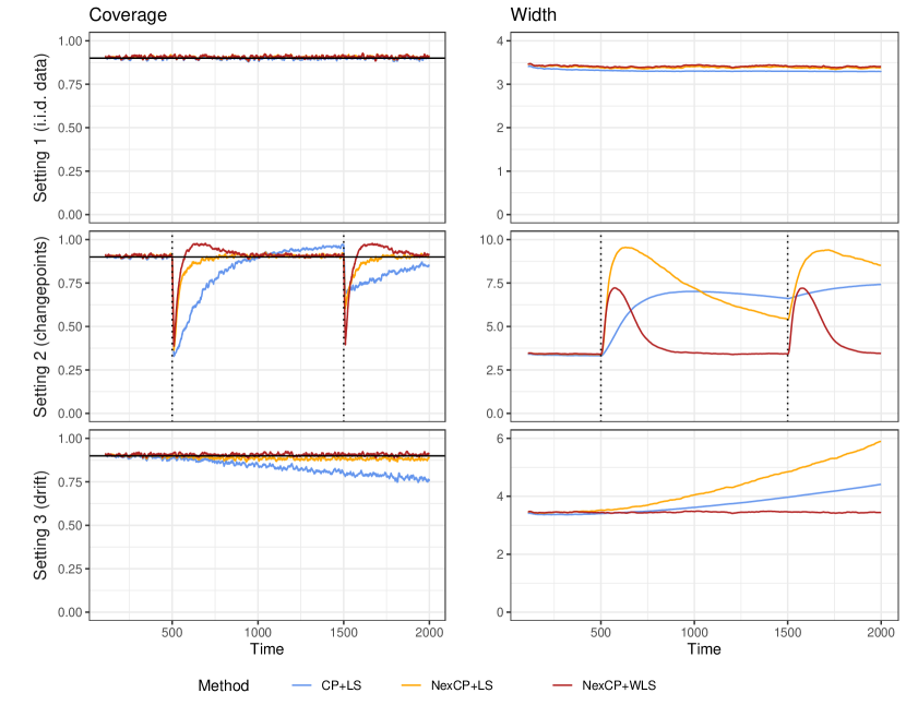
Figure 2: Simulation results showing mean prediction interval coverage and width, averaged over 200 independent trials. The displayed curves are smoothed by taking a rolling average with a window of 10 time points.

Our results are shown in Figure 2, and are summarized in Table 1. In terms of coverage, we see that all three methods have coverage $\approx 90\%$ across the time range of the experiment for the i.i.d. data setting (Setting 1), while for the changepoint (Setting 2) and distribution drift (Setting 3) experiments, the two proposed methods achieve approximately the desired coverage level, but the original full conformal method CP+LS undercovers. In particular, as expected, CP+LS shows steep drops in coverage in Setting 2 after changepoints, while in Setting 3 the coverage for CP+LS declines gradually over time as the distribution drift grows. The NexCP+LS and NexCP+WLS methods are better able to maintain coverage in these settings. (In fact, in Setting 2, we see that NexCP+WLS overcovers for a period of time after each changepoint—this is because, a short period of time after the changepoint, the fitted weighted least squares model is already quite accurate for the new data distribution, but the weights $\tilde{w}_{i}$ are still placing some weight on residuals from data points from before the changepoint, leading briefly to an overestimate of our model error.)

	Setting 1 (i.i.d. data)		Setting 2 (changepoints)		Setting 3 (drift)
	Coverage	Width	Coverage	Width	Coverage	Width
CP+LS	0.900	3.31	0.835	5.99	0.838	3.73
NexCP+LS	0.907	3.39	0.884	6.83	0.888	4.29
NexCP+WLS	0.907	3.42	0.906	4.13	0.907	3.45

Table 1: Simulation results showing mean prediction interval coverage and width, averaged over all time points and over 200 trials.

Turning to the prediction interval width, for the i.i.d. data setting (Setting 1), the three methods show similar mean widths, although the widths for NexCP+LS and NexCP+WLS are very slightly higher than for CP+LS; in addition, variability is higher for NexCP+LS and NexCP+WLS than for CP+LS, which is to be expected since using decaying weights $w_{i}$ for computing the prediction intervals leads to a lower effective sample size. For the changepoint (Setting 2) and distribution drift (Setting 3) experiments, we see that NexCP+LS leads to wider prediction intervals than the original method CP+LS, which is to be expected since NexCP+LS is using the same model fitting algorithm but avoiding the undercoverage issue of CP+LS. More importantly, NexCP+WLS is able to construct narrower prediction intervals than CP+LS, while avoiding undercoverage. This is due to the fact that weighted least squares leads to more accurate fitted models. This highlights the utility of nonsymmetric algorithms for settings where data are not exchangeable.

5.2 Electricity data set

We now compare the three methods on a real data set. The ELEC2 data set (Harries, 1999) tracks electricity usage and pricing in the states of New South Wales and Victoria in Australia, every 30 minutes over a 2.5 year period in 1996–1999. (This data set was previously analyzed by Vovk et al. (2021) in the context of conformal prediction, finding distribution drift that violated exchangeability.)

For our experiment, we use four covariates: nswprice and vicprice, the price of electricity in each of the two states, and nswdemand and vicdemand, the usage demand in each of the two states. Our response variable is transfer, the quantity of electricity transferred between the two states. We work with a subset of the data, keeping only those observations in the time range 9:00am–12:00pm (aiming to remove daily fluctuation effects), and discarding an initial stretch of time during which the value transfer is constant. After these steps, we have $N=3444$ time points. We then implement the same three methods as in the simulations (CP+LS, NexCP+LS, and NexCP+WLS), using the exact same definitions and settings as before.

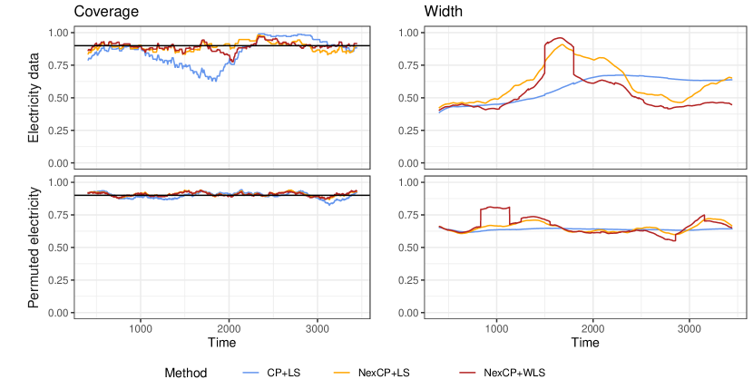
Figure 3: Electricity data results showing coverage and prediction interval width on the original data and the permuted data. The displayed curves are smoothed by taking a rolling average with a window of 300 time points.

Our goal is to examine how distribution drift over the duration of this 2.5 year period will affect each of the three methods. As a sort of “control group”, we also perform the experiment with a permuted version of this same data set—we draw a permutation $\pi$ on $[N]$ uniformly at random, and then repeat the same experiment on the permuted data set $(X_{\pi(1)},Y_{\pi(1)}),\dots,(X_{\pi(N)},Y_{\pi(N)})$. The random permutation ensures that the distribution of this data set now satisfies exchangeability.

Our results are shown in Figure 3, and summarized in Table 2. On the original data set, we see that the unweighted method CP+LS shows some undercoverage, while both NexCP+LS and NexCP+WLS achieve nearly the desired $90\%$ coverage level. In particular, CP+LS shows undercoverage during a long range of time around the middle of the duration of the experiment, and then recovers, showing the effects of distribution drift in this data set—this occurs as the response variable transfer is more noisy during the middle of the time range, as compared to the beginning and end of the time range. On the permuted data set, on the other hand, all three methods show coverage that is close to $90\%$ throughout the time range, which is expected since the permuted data set is exchangeable.

	Electricity data		Permuted electricity data
	Coverage	Width	Coverage	Width
CP+LS	0.852	0.565	0.899	0.639
NexCP+LS	0.890	0.606	0.908	0.652
NexCP+WLS	0.893	0.527	0.908	0.663

Table 2: Electricity data results showing coverage and prediction interval width on the original data and the permuted data, averaged over all time points.

Turning now to prediction interval width, on the original data set we see that the interval width of NexCP+LS is generally larger than that of NexCP+WLS, again demonstrating the advantage of a nonsymmetric algorithm. For the permuted data set, on the other hand, the interval widths are similar, although NexCP+LS and NexCP+WLS show higher variability; this is explained by the lower effective sample size that is introduced by weighting the data points, combined with the heavy-tailed nature of the data.

5.3 Election data set

Finally, we apply our weighted methods to predict how Americans voted in the 2020 U.S. presidential election. Our experiments in this subsection are inspired by the work of Cherian and Bronner (2020) for The Washington Post.

The left map in Figure 4 shows, county by county, the relative change in the number of votes for the Democratic Candidate between 2016 and 2020, defined as:

$$Y=\frac{\textnormal{Dem}_{2020}-\text{Dem}_{2016}}{\textnormal{Dem}_{2016}},$$

where $\textnormal{Dem}_{2020}$ is the number of Democratic votes in a given county in 2020 (and similarly for 2016). In our experiments, the covariate vector $X$ includes information on the makeup of the county population by ethnicity, age, sex, median income and education (see Appendix G for details and for information about the data sources), given the data that was available in 2020.

During real-time election forecasting, after observing the response $Y$ for a subset of the counties (those counties that have reported), the problem is to predict the vote change $Y$ in each of the counties where vote counts are not yet available. If the order in which counties report their vote totals were drawn uniformly at random, then the exchangeability of the resulting training and test sets would mean that conformal prediction can be applied in a straightforward manner to obtain valid predictive intervals for the unobserved counties. In practice, however, the time at which a county reports its votes may depend on various factor such as the time zone of the county, the size of the county, and so on. Therefore, if at any point in time we were to train on counties whose votes have already been reported, then this can create a division of training and test sets that violates exchangeability, and can thus lead to a failure of the predictive coverage guarantee.

To mimic this type of biased split, for the current experiment, we use counties that fall under the Eastern time zone as our training set, and the remaining counties as the test set, as highlighted in the right-hand map in Figure 4. This results in 1119 training points and 1957 test points.

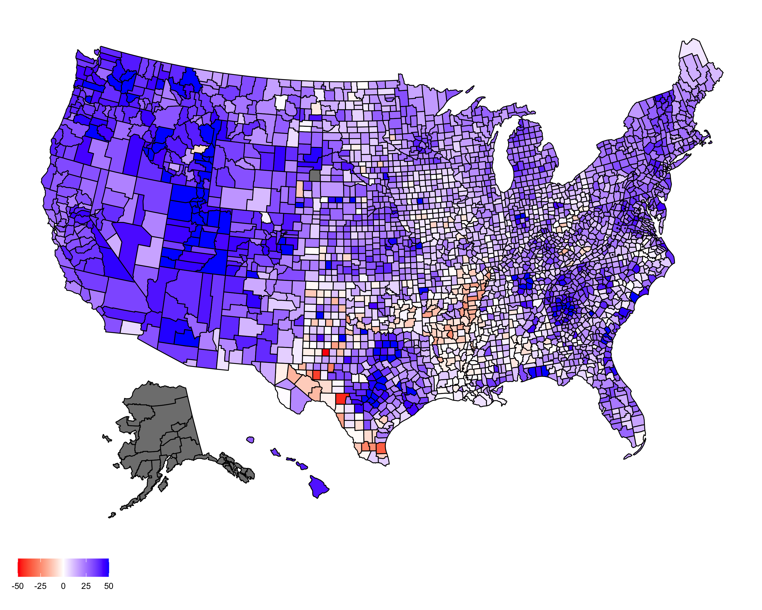
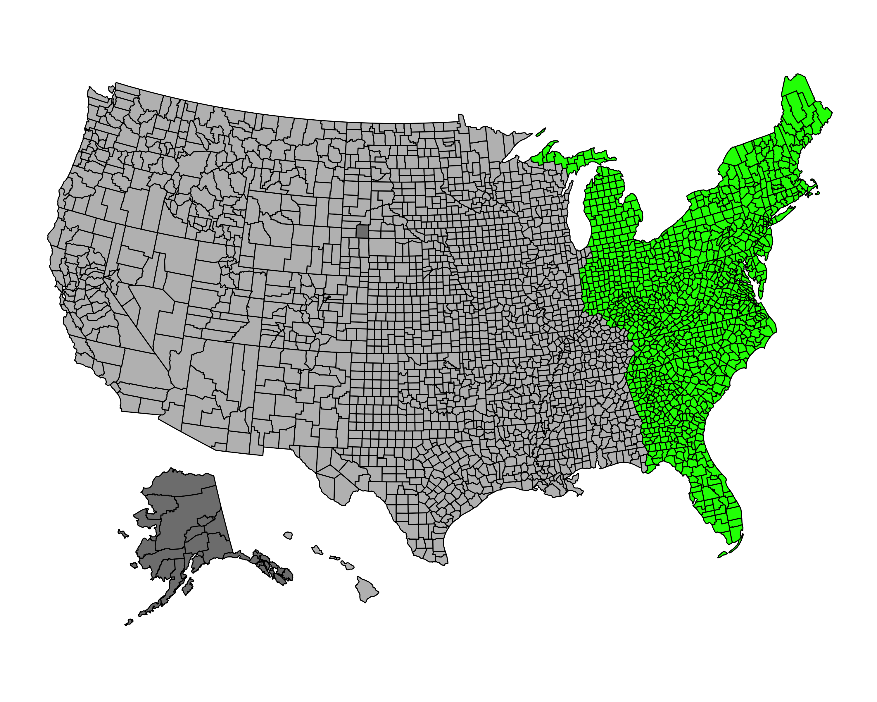
Figure 4: Left map: relative change in the number of votes for the Democratic presidential candidate from 2016 to 2020. Blue colors indicate an increase in Democratic votes and red colors indicate a decrease, with the darkest shade of blue (respectively, red) corresponding to a 50% increase (respectively, decrease). Right map: the counties that form the training set (in green), and all remaining counties are in the test set.

To run the experiment, we implement the same three full conformal methods as before (CP+LS, NexCP+LS, and NexCP+WLS). To define weights $w_{i}$ for NexCP, we will use some available side information—namely, $X^{\textnormal{prev}}\in\mathbb{R}^{p}$, which gives the 2016 measurements for the same set of demographic and socioeconomic variables as contained in $X$ for 2020. The weights are then defined as $w_{i}=e^{-\gamma\|X^{\textnormal{prev}}_{i}-X^{\textnormal{prev}}_{n+1}\|_{2}}$, where we choose $\gamma$ to satisfy

$$\frac{(\sum_{i=1}^{n}w_{i}+1)^{2}}{\sum_{i=1}^{n}w_{i}^{2}+1}=100,$$

essentially corresponding to an effective training sample size of $100$ once we use the weighted training sample. We note that, since these weights depend only on data from 2016, we can treat these weights as fixed (i.e., these weights were determined “earlier” than gathering the data set $\{(X_{i},Y_{i})\}_{i=1}^{3076}$ in 2020). By using these weights within nonexchangeable conformal, we are implicitly invoking a hypothesis that counties which had similar demographics in 2016 will generate approximately exchangeable data in 2020. Finally, for NexCP+WLS, we use the same choice for the tags used for running the weighted least squares regression, i.e., setting $t_{i}=w_{i}$.

In addition, we also repeat the entire experiment with quantile regression in place of linear regression, and use a corresponding choice of the nonconformity score function—specifically, after fitting a lower 5% percentile function $\hat{q}_{0.05}(\cdot)$, and an upper 95% percentile function $\hat{q}_{0.95}(\cdot)$ to the data, the nonconformity score is given by $\widehat{S}(X_{i},Y_{i})=\max\{\hat{q}_{0.05}(X_{i})-Y_{i},Y_{i}-\hat{q}_{0.95}(X_{i})\}$, as in Romano et al. (2019). This yields three additional methods: conformal prediction with quantile regression (CP+QR), nonexchangeable conformal with quantile regression (NexCP+QR), and nonexchangeable conformal with weighted quantile regression (NexCP+WQR), where the weights $w_{i}$ and the tags $t_{i}$ are defined the same way as in linear regression.

Table 3 shows the resulting predictive coverage, averaged over the test set, for each of the three methods, when they are run with target coverage level $1-\alpha=0.9$. We can see that CP undercovers substantially, particularly when combined with least squares, due to the construction of nonexchangeable training and test counties. In contrast, NexCP (with or without the nonsymmetric algorithm) is able to achieve a coverage level that is much closer to the target level $90\%$.

	Coverage
CP+LS	0.743
NexCP+LS	0.820
NexCP+WLS	0.840

	Coverage
CP+QR	0.782
NexCP+QR	0.836
NexCP+WQR	0.835

Table 3: Election data results showing coverage, averaged over all test counties.

6 Proofs

In this section, we give proofs of all theorems presented so far.

6.1 Background: proof of Theorem 1

To help build intuition for the proof techniques we will use later on, we reformulate Vovk et al. (2005)’s proofs of these results, and we then explain some of the challenges in extending these existing results to our new setting.

Let $R_{i}=R^{Y_{n+1}}_{i}$ denote the $i$th residual, at the hypothesized value $y=Y_{n+1}$. By our assumptions, the data points $(X_{1},Y_{1}),\dots,(X_{n+1},Y_{n+1})$ are i.i.d. (or exchangeable), and the fitted model $\widehat{\mu}=\widehat{\mu}^{Y_{n+1}}=\mathcal{A}((X_{1},Y_{1}),\dots,(X_{n+1},Y_{n+1}))$ is constructed via an algorithm $\mathcal{A}$ that treats these $n+1$ data points symmetrically. The residuals $R_{i}=|Y_{i}-\widehat{\mu}(X_{i})|$ are thus exchangeable.

Now define the set of “strange” points

$$\mathcal{S}(R)=\left\{i\in[n+1]\ :\ R_{i}>\mathsf{Q}_{1-\alpha}\left(\sum_{j=1}^{n+1}\frac{1}{n+1}\cdot\delta_{R_{j}}\right)\right\}.$$

That is, an index $i$ corresponds to a “strange” point if its residual $R_{i}$ is one of the $\lfloor\alpha(n+1)\rfloor$ largest elements of the list $R_{1},\dots,R_{n+1}$. By definition, this can include at most $\alpha(n+1)$ entries of the list, i.e.,

$$|\mathcal{S}(R)|\leq\alpha(n+1).$$

Next, by definition of the full conformal prediction set, we see that $Y_{n+1}\not\in\widehat{C}_{n}(X_{n+1})$ (i.e., coverage fails) if and only if $R_{n+1}>\mathsf{Q}_{1-\alpha}\left(\sum_{i=1}^{n+1}\frac{1}{n+1}\cdot\delta_{R_{i}}\right)$, or equivalently, if and only if the test point $n+1$ is “strange”, i.e., $n+1\in\mathcal{S}(R)$. Therefore, we have

$$\mathbb{P}\left\{{Y_{n+1}\not\in\widehat{C}_{n}(X_{n+1})}\right\}=\mathbb{P}\left\{{n+1\in\mathcal{S}(R)}\right\}=\frac{1}{n+1}\sum_{i=1}^{n+1}\mathbb{P}\left\{{i\in\mathcal{S}(R)}\right\}\\ =\frac{1}{n+1}\mathbb{E}\left[{\sum_{i=1}^{n+1}{\mathbbm{1}}\left\{{i\in\mathcal{S}(R)}\right\}}\right]=\frac{1}{n+1}\mathbb{E}\left[{|\mathcal{S}(R)|}\right]\leq\frac{1}{n+1}\cdot\alpha(n+1)=\alpha,$$

where the second equality holds due to the exchangeability of $R_{1},\dots,R_{n+1}$.

Challenges for the new algorithms.

We will now see why the above proof does not obviously extend to our nonexchangeable conformal method, even if we were to assume that the data points $(X_{i},Y_{i})$ are exchangeable. First, suppose that $\mathcal{A}$ is symmetric (i.e., we do not use tags $t_{i}$). For the original full conformal prediction method, in the proof of Theorem 1, exchangeability of the data points is used to verify that $\mathbb{P}\left\{{n+1\in\mathcal{S}(R)}\right\}=\mathbb{P}\left\{{i\in\mathcal{S}(R)}\right\}$ for each $i\in[n]$, or equivalently,

$$\mathbb{P}\left\{{R_{n+1}>\mathsf{Q}_{1-\alpha}\left(\sum_{j=1}^{n+1}\tfrac{1}{n+1}\cdot\delta_{R_{j}}\right)}\right\}=\mathbb{P}\left\{{R_{i}>\mathsf{Q}_{1-\alpha}\left(\sum_{j=1}^{n+1}\tfrac{1}{n+1}\cdot\delta_{R_{j}}\right)}\right\}.$$

This equality holds since the residuals $R_{i}$ are exchangeable (by assumption on the data) and since $\mathsf{Q}_{1-\alpha}(\sum_{j=1}^{n+1}\frac{1}{n+1}\cdot\delta_{R_{j}})$ is a symmetric function of $R_{1},\dots,R_{n+1}$. For the nonexchangeable full conformal algorithm proposed in (12), on the other hand, we would need to check whether

$$\mathbb{P}\left\{{R_{n+1}>\mathsf{Q}_{1-\alpha}\left(\sum_{j=1}^{n+1}\tilde{w}_{j}\cdot\delta_{R_{j}}\right)}\right\}\stackrel{{\scriptstyle\textnormal{\normalsize?}}}{{=}}\mathbb{P}\left\{{R_{i}>\mathsf{Q}_{1-\alpha}\left(\sum_{j=1}^{n+1}\tilde{w}_{j}\cdot\delta_{R_{j}}\right)}\right\}.$$

Even when the residuals $R_{i}$ are exchangeable (i.e., when the data points are exchangeable and the algorithm is symmetric), the weighted quantile $\mathsf{Q}_{1-\alpha}(\sum_{j=1}^{n+1}\tilde{w}_{j}\cdot\delta_{R_{j}})$ is no longer a symmetric function of $R_{1},\dots,R_{n+1}$ if the weights $\tilde{w}_{j}$ are not all equal, and therefore, the equality will no longer be true in general.

Next, if we use nonsymmetric algorithms that take tagged data points $(X_{i},Y_{i},t_{i})$ as input, the situation becomes even more complex—even if the data points $(X_{i},Y_{i})$ are exchangeable, the residuals $R_{1},\dots,R_{n+1}$ may no longer be exchangeable as they depend on a fitted model $\widehat{\mu}$ that treats the training data points nonsymmetrically.

Finally, in this paper we are of course primarily interested in the setting where the data points are no longer exchangeable, and in bounding the resulting coverage gap. This leads to additional challenges, all of which we address in the proofs below.

6.2 Proof of Theorem 2

Since nonexchangeable split conformal is simply a special case of nonexchangeable full conformal, we only need to prove the result for full conformal.

For each $k\in[n+1]$, denote

$$\widehat{\mu}^{k}=\widehat{\mu}^{Y_{n+1},k}=\mathcal{A}\Big{(}(X_{\pi_{k}(1)},Y_{\pi_{k}(1)},t_{1}),\dots,(X_{\pi_{k}(n+1)},Y_{\pi_{k}(n+1)},t_{n+1})\Big{)},$$

where for any $k\in[n]$, as before $\pi_{k}$ denotes the permutation on $[n+1]$ that swaps indices $k$ and $n+1$, while $\pi_{n+1}$ is the identity permutation. Then, for any $k\in[n+1]$, we can calculate

$$\big{(}R(Z^{k})\big{)}_{i}=|Y_{\pi_{k}(i)}-\widehat{\mu}^{k}(X_{\pi_{k}(i)})|,$$

and therefore,

$$\big{(}R(Z^{K})\big{)}_{i}=\begin{cases}R^{Y_{n+1},K}_{i},&\textnormal{if }i\not=K\textnormal{ and }i\not=n+1,\\ R^{Y_{n+1},K}_{n+1},&\textnormal{if }i=K,\\ R^{Y_{n+1},K}_{K},&\textnormal{if }i=n+1.\end{cases}$$ (20)

The definition of the nonexchangeable full conformal prediction set (18) reveals

$$Y_{n+1}\not\in\widehat{C}_{n}(X_{n+1})\ \iff\ R^{Y_{n+1},K}_{n+1}>\mathsf{Q}_{1-\alpha}\left(\sum_{i=1}^{n+1}\tilde{w}_{i}\cdot\delta_{R^{Y_{n+1},K}_{i}}\right),$$

and we can equivalently write this as

$$Y_{n+1}\not\in\widehat{C}_{n}(X_{n+1})\ \iff\ R^{Y_{n+1},K}_{n+1}>\mathsf{Q}_{1-\alpha}\left(\sum_{i=1}^{n}\tilde{w}_{i}\cdot\delta_{R^{Y_{n+1},K}_{i}}+\tilde{w}_{n+1}\cdot\delta_{+\infty}\right).$$ (21)

Next, we verify that deterministically (20) implies

$$\mathsf{Q}_{1-\alpha}\left(\sum_{i=1}^{n}\tilde{w}_{i}\cdot\delta_{R^{Y_{n+1},K}_{i}}+\tilde{w}_{n+1}\cdot\delta_{+\infty}\right)\geq\mathsf{Q}_{1-\alpha}\left(\sum_{i=1}^{n+1}\tilde{w}_{i}\cdot\delta_{(R(Z^{K}))_{i}}\right).$$ (22)

Indeed, if $K=n+1$, then $R(Z^{K})=R^{Y_{n+1},K}$ by (20), and so the bound holds trivially. If instead $K\leq n$, then the distribution on the left-hand side of (22) equals

$$\sum_{i=1}^{n}\tilde{w}_{i}\cdot\delta_{R^{Y_{n+1},K}_{i}}+\tilde{w}_{n+1}\cdot\delta_{+\infty}\\ =\sum_{i=1,\dots,n;i\neq K}\tilde{w}_{i}\cdot\delta_{R^{Y_{n+1},K}_{i}}+\tilde{w}_{K}(\delta_{R^{Y_{n+1},K}_{K}}+\delta_{+\infty})+(\tilde{w}_{n+1}-\tilde{w}_{K})\delta_{+\infty},$$

while the distribution on the right-hand side of (22) can be rewritten as

$$\sum_{i=1}^{n+1}\tilde{w}_{i}\cdot\delta_{(R(Z^{K}))_{i}}=\sum_{i=1,\dots,n;i\neq K}\tilde{w}_{i}\cdot\delta_{R^{Y_{n+1},K}_{i}}+\tilde{w}_{K}\delta_{R^{Y_{n+1},K}_{n+1}}+\tilde{w}_{n+1}\delta_{R^{Y_{n+1},K}_{K}}\\ =\sum_{i=1,\dots,n;i\neq K}\tilde{w}_{i}\cdot\delta_{R^{Y_{n+1},K}_{i}}+\tilde{w}_{K}(\delta_{R^{Y_{n+1},K}_{K}}+\delta_{R^{Y_{n+1},K}_{n+1}})+(\tilde{w}_{n+1}-\tilde{w}_{K})\delta_{R^{Y_{n+1},K}_{K}},$$

by applying (20). Since $w_{K}\in[0,1]$ by assumption, we have $\tilde{w}_{n+1}\geq\tilde{w}_{K}$, which from the last two displays verifies that (22) must hold. Combining (21) and (22), we have

$$Y_{n+1}\not\in\widehat{C}_{n}(X_{n+1})\ \implies\ R^{Y_{n+1},K}_{n+1}>\mathsf{Q}_{1-\alpha}\left(\sum_{i=1}^{n+1}\tilde{w}_{i}\cdot\delta_{(R(Z^{K}))_{i}}\right),$$

or equivalently by (20),

$$Y_{n+1}\not\in\widehat{C}_{n}(X_{n+1})\ \implies\ (R(Z^{K}))_{K}>\mathsf{Q}_{1-\alpha}\left(\sum_{i=1}^{n+1}\tilde{w}_{i}\cdot\delta_{(R(Z^{K}))_{i}}\right).$$ (23)

Next define a function $\mathcal{S}$ from $\mathbb{R}^{n+1}$ to subsets of $[n+1]$, as follows: for any $r\in\mathbb{R}^{n+1}$,

$$\mathcal{S}(r)=\left\{i\in[n+1]\ :\ r_{i}>\mathsf{Q}_{1-\alpha}\left(\sum_{j=1}^{n+1}\tilde{w}_{j}\cdot\delta_{r_{j}}\right)\right\}.$$ (24)

These are the “strange” points—indices $i$ for which $r_{i}$ is unusually large, relative to the (weighted) empirical distribution of $r_{1},\dots,r_{n+1}$. A direct argument (see, e.g., the deterministic inequality in (Harrison, 2012, Lemma A.1)) shows that

$$\sum_{i\in\mathcal{S}(r)}\tilde{w}_{i}\leq\alpha\textnormal{ for all $r\in\mathbb{R}^{n+1}$},$$ (25)

that is, the (weighted) fraction of “strange” points cannot exceed $\alpha$. From (23), we have that noncoverage of $Y_{n+1}$ implies strangeness of point $K$:

$$Y_{n+1}\not\in\widehat{C}_{n}(X_{n+1})\ \implies\ K\in\mathcal{S}\big{(}R(Z^{K})\big{)}.$$ (26)

Finally,

$$\mathbb{P}\left\{{K\in\mathcal{S}\big{(}R(Z^{K})\big{)}}\right\} =\sum_{i=1}^{n+1}\mathbb{P}\left\{{K=i\textnormal{ and }i\in\mathcal{S}\big{(}R(Z^{i})\big{)}}\right\}$$

$$=\sum_{i=1}^{n+1}\tilde{w}_{i}\cdot\mathbb{P}\left\{{i\in\mathcal{S}\big{(}R(Z^{i})\big{)}}\right\}$$ (27)

$$\leq\sum_{i=1}^{n+1}\tilde{w}_{i}\cdot\left(\mathbb{P}\left\{{i\in\mathcal{S}\big{(}R(Z)\big{)}}\right\}+\mathsf{d}_{\mathsf{TV}}\big{(}R(Z),R(Z^{i})\big{)}\right)$$

$$=\mathbb{E}\left[{\sum_{i\in\mathcal{S}(R(Z))}\tilde{w}_{i}}\right]+\sum_{i=1}^{n}\tilde{w}_{i}\cdot\mathsf{d}_{\mathsf{TV}}\big{(}R(Z),R(Z^{i})\big{)}$$

$$\leq\alpha+\sum_{i=1}^{n}\tilde{w}_{i}\cdot\mathsf{d}_{\mathsf{TV}}\big{(}R(Z),R(Z^{i})\big{)},$$

where the last step holds by (25), whereas step (27) holds because $K\mathchoice{\mathrel{\hbox to0.0pt{$\displaystyle\perp$\hss}\mkern 2.0mu{\displaystyle\perp}}}{\mathrel{\hbox to0.0pt{$\textstyle\perp$\hss}\mkern 2.0mu{\textstyle\perp}}}{\mathrel{\hbox to0.0pt{$\scriptstyle\perp$\hss}\mkern 2.0mu{\scriptstyle\perp}}}{\mathrel{\hbox to0.0pt{$\scriptscriptstyle\perp$\hss}\mkern 2.0mu{\scriptscriptstyle\perp}}}Z$ and $Z^{i}=\pi_{i}(Z)$ is a function of the data $Z$, and therefore, $K\mathchoice{\mathrel{\hbox to0.0pt{$\displaystyle\perp$\hss}\mkern 2.0mu{\displaystyle\perp}}}{\mathrel{\hbox to0.0pt{$\textstyle\perp$\hss}\mkern 2.0mu{\textstyle\perp}}}{\mathrel{\hbox to0.0pt{$\scriptstyle\perp$\hss}\mkern 2.0mu{\scriptstyle\perp}}}{\mathrel{\hbox to0.0pt{$\scriptscriptstyle\perp$\hss}\mkern 2.0mu{\scriptscriptstyle\perp}}}Z^{i}$.

7 Discussion

Our main contribution in this paper was to demonstrate how conformal prediction, which has crucially relied on exchangeability, can be modified to handle nonsymmetric regression algorithms, and utilize weighted residual distributions in order to provide robustness against deviations from exchangeability in the data. With no assumptions whatsoever on the underlying joint distribution of the data, it is possible to give a coverage guarantee for both existing conformal methods, and our new proposed nonexchangeable conformal procedures. The coverage gap, expressing the extent to which the guaranteed coverage level is lower than what would be guaranteed under exchangeability, is bounded by a weighted sum of total variation distances between the residual vectors obtained by swapping the $i$th point with the $(n+1)$st point.

Our work opens the door to applying conformal prediction in applications where the data is globally likely far from exchangeable but locally deviates mildly from exchangeability. Tags and weights can be prudently used to downweight “far away” points during training and calibration, and recover reasonable coverage in practice. We hope our work will lead to more targeted methods that focus on custom design of nonsymmetric algorithms and weighting schemes to improve efficiency and robustness in specific applications, through the lens of nonexchangeable conformal prediction.

Appendix A Extension to general nonconformity scores

In this section, we extend our new nonexchangeable inference methods for split and full conformal to the setting of general nonconformity scores. The response is no longer required to be real-valued, so we will consider the general setting with data points $(X_{i},Y_{i})\in\mathcal{X}\times\mathcal{Y}$.

For split conformal, as usual, we assume that the nonconformity score function $\widehat{S}:\mathcal{X}\times\mathcal{Y}\rightarrow\mathbb{R}$ is pre-fitted. The nonexchangeable split conformal set is given by

$$\widehat{C}_{n}(X_{n+1})=\left\{y\in\mathcal{Y}:\widehat{S}(X_{n+1},y)\leq\mathsf{Q}_{1-\alpha}\left(\sum_{i=1}^{n}\tilde{w}_{i}\cdot\delta_{\widehat{S}(X_{i},Y_{i})}+\tilde{w}_{n+1}\cdot\delta_{+\infty}\right)\right\}.$$ (28)

For the special case $\widehat{S}(x,y)=|y-\widehat{\mu}(x)|$ (where $\widehat{\mu}$ is a pre-fitted function), note that this reduces to the previous definition (11) from before.

For full conformal, we now consider algorithms $\mathcal{A}$ of the form

$$\mathcal{A}:\ \cup_{n\geq 0}\left(\mathcal{X}\times\mathcal{Y}\times\mathcal{T}\right)^{n}\ \rightarrow\ \left\{\textnormal{measurable functions $\widehat{S}:\mathcal{X}\times\mathcal{Y}\rightarrow\mathbb{R}$}\right\}.$$ (29)

(As before, the symmetric algorithm setting, with no tags $t_{i}$, is simply a special case of this general formulation.) First, for any $y\in\mathbb{R}$ and any $k\in[n+1]$, define

$$\widehat{S}^{y,k}=\mathcal{A}\left((X_{\pi_{k}(i)},Y^{y}_{\pi_{k}(i)},t_{i}):i\in[n+1]\right),$$

where the permutation $\pi_{k}$ is defined as before (that swaps indices $k$ and $n+1$), and where

$$Y^{y}_{i}=Y_{i},\ i=1,\ldots,n,\quad Y^{y}_{n+1}=y,$$

as before. Define the scores from this model,

$$S^{y,k}_{i}=\widehat{S}^{y,k}(X_{i},Y_{i}),\ i=1,\dots,n,\quad S^{y,k}_{n+1}=\widehat{S}^{y,k}(X_{n+1},y).$$

Then, after drawing a random index $K$ as in (17), the prediction set is given by

$$\widehat{C}_{n}(X_{n+1})=\left\{y\in\mathcal{Y}:S^{y,K}_{n+1}\leq\mathsf{Q}_{1-\alpha}\left(\sum_{i=1}^{n+1}\tilde{w}_{i}\cdot\delta_{S^{y,K}_{i}}\right)\right\}.$$ (30)

For the special case $\widehat{S}(x,y)=|y-\widehat{\mu}(x)|$ (where $\widehat{\mu}$ is fitted on the same data), this again reduces to the previous definition (18) from before.

Importantly, the same theoretical result (i.e., Theorem 2) holds for these more general methods as well. The proof does not fundamentally rely on residual scores, and the modifications required for the general case are straightforward, so we omit the details here.

Appendix B Nonexchangeable jackknife+

B.1 Background

The jackknife+ [Barber et al., 2021] (closely related to “cross-conformal prediction” [Vovk, 2015]) is a method that offers a compromise between the computational and statistical costs of the split and full conformal methods. For each $i=1,\dots,n$, define the $i$th leave-one-out model as

$$\widehat{\mu}_{-i}=\mathcal{A}\big{(}(X_{1},Y_{1}),\dots,(X_{i-1},Y_{i-1}),(X_{i+1},Y_{i+1}),\dots,(X_{n},Y_{n})\big{)},$$ (31)

fitted to the training data with $i$th point removed. Define also the $i$th leave-one-out residual $R_{i}^{\textnormal{LOO}}=|Y_{i}-\widehat{\mu}_{-i}(X_{i})|$, which avoids overfitting since data point $(X_{i},Y_{i})$ is not used for training $\widehat{\mu}_{-i}$. The jackknife+ prediction interval is then given by

$$\Bigg{[}\mathsf{Q}_{\alpha}\left(\sum_{i=1}^{n}\tfrac{1}{n+1}\cdot\delta_{\widehat{\mu}_{-i}(X_{n+1})-R^{\textnormal{LOO}}_{i}}+\tfrac{1}{n+1}\cdot\delta_{-\infty}\right),\\ \mathsf{Q}_{1-\alpha}\left(\sum_{i=1}^{n}\tfrac{1}{n+1}\cdot\delta_{\widehat{\mu}_{-i}(X_{n+1})+R^{\textnormal{LOO}}_{i}}+\tfrac{1}{n+1}\cdot\delta_{+\infty}\right)\Bigg{]}.$$ (32)

While in practice the jackknife+ generally provides coverage close to the target level $1-\alpha$ (and provably so under a stability assumption on $\mathcal{A}$), its theoretical guarantee only ensures $1-2\alpha$ probability of coverage in the worst case:

Theorem 4 (Jackknife+ [Barber et al., 2021]).

If $(X_{1},Y_{1}),\dots,(X_{n},Y_{n}),(X_{n+1},Y_{n+1})$ are i.i.d. (or more generally, exchangeable), and the algorithm $\mathcal{A}$ treats the input data points symmetrically as in (6), then the jackknife+ prediction interval defined in (32) satisfies

$$\mathbb{P}\left\{{Y_{n+1}\in\widehat{C}_{n}(X_{n+1})}\right\}\geq 1-2\alpha.$$

This method can be viewed as a form of $n$-fold cross-validation; more generally, the CV+ method [Barber et al., 2021] uses $K$-fold cross-validation for any desired $K$, and obtains a similar distribution-free guarantee.

B.2 Methods

We next present the nonexchangeable jackknife+ method.

Nonexchangeable jackknife+ with a symmetric algorithm.

We first consider the setting where the algorithm $\mathcal{A}$ is symmetric. To begin, we choose weights $w_{i}\in[0,1]$, $i=1,\dots,n$, which are fixed ahead of time, and as before, this gives rise to normalized weights as in (10). The prediction interval is then given by

$$\Bigg{[}\mathsf{Q}_{\alpha}\left(\sum_{i=1}^{n}\tilde{w}_{i}\cdot\delta_{\widehat{\mu}_{-i}(X_{n+1})-R^{\textnormal{LOO}}_{i}}+\tilde{w}_{n+1}\cdot\delta_{-\infty}\right),\\ \mathsf{Q}_{1-\alpha}\left(\sum_{i=1}^{n}\tilde{w}_{i}\cdot\delta_{\widehat{\mu}_{-i}(X_{n+1})+R^{\textnormal{LOO}}_{i}}+\tilde{w}_{n+1}\cdot\delta_{+\infty}\right)\Bigg{]},$$ (33)

where $\widehat{\mu}_{-i}$ is defined as in (31), and $R^{\textnormal{LOO}}_{i}=|Y_{i}-\widehat{\mu}_{-i}(X_{i})|$ as before.

Analogous to split and full conformal, here the original (unweighted) version of jackknife+ is recovered by choosing weights $w_{1}=\dots=w_{n}=1$ in the new algorithm.

Nonexchangeable jackknife+ with a nonsymmetric algorithm.

We now extend the nonexchangeable jackknife+ to allow for a nonsymmetric algorithm $\mathcal{A}$. For any $k\in[n+1]$ and any $i\in[n]$, define the model $\widehat{\mu}^{k}_{-i}$ as

$$\widehat{\mu}^{k}_{-i}=\mathcal{A}\left((X_{\pi_{k}(j)},Y_{\pi_{k}(j)},t_{j}):j\in[n+1],\pi_{k}(j)\not\in\{i,n+1\}\right).$$

As before, $\pi_{k}$ is the permutation on $[n+1]$ that swaps indices $k$ and $n+1$ (or, the identity permutation in the case $k=n+1$). Equivalently,

$$\widehat{\mu}^{k}_{-i}=\begin{cases}\mathcal{A}\left((X_{j},Y_{j},t_{j}):j\in[n]\backslash\{i,k\},(X_{k},Y_{k},t_{n+1})\right),&\textnormal{ if }k\in[n]\textnormal{ and }k\neq i,\\ \mathcal{A}\left((X_{j},Y_{j},t_{j}):j\in[n]\backslash\{i\}\right),&\textnormal{ if }k=n+1\textnormal{ or }k=i.\end{cases}$$

In other words, this model is fitted on the training data $(X_{1},Y_{1}),\dots,(X_{n},Y_{n})$ but with the $i$th point removed, and furthermore the data point $(X_{k},Y_{k})$ is given the tag $t_{n+1}$ rather than $t_{k}$. (We note that computing the fitted model $\widehat{\mu}^{k}_{-i}$ does not require knowledge of the test point $(X_{n+1},Y_{n+1})$, because $\pi_{k}(j)=n+1$ is excluded from the data set when running $\mathcal{A}$.) For the model $\widehat{\mu}^{k}_{-i}$, we define its corresponding leave-one-out residuals as

$$R^{k,\textnormal{LOO}}_{i}=|Y_{i}-\widehat{\mu}^{k}_{-i}(X_{i})|.$$

To run the method, we first draw a random index $K$ as in (17), and then compute the nonexchangeable jackknife+ prediction interval as

$$\Bigg{[}\mathsf{Q}_{\alpha}\left(\sum_{i=1}^{n}\tilde{w}_{i}\cdot\delta_{\widehat{\mu}^{K}_{-i}(X_{n+1})-R^{K,\textnormal{LOO}}_{i}}+\tilde{w}_{n+1}\cdot\delta_{-\infty}\right),\\ \mathsf{Q}_{1-\alpha}\left(\sum_{i=1}^{n}\tilde{w}_{i}\cdot\delta_{\widehat{\mu}^{K}_{-i}(X_{n+1})+R^{K,\textnormal{LOO}}_{i}}+\tilde{w}_{n+1}\cdot\delta_{+\infty}\right)\Bigg{]}.$$ (34)

Again, as was the case for nonexchangeable conformal, this method is a generalization of the symmetric case for nonexchangeable jackknife+, which was presented above.

B.3 Theory

As for the proof for nonexchangeable full conformal, we first need to define how we map a data sequence $z=(z_{1},\dots,z_{n+1})\in(\mathcal{X}\times\mathbb{R})^{n+1}$, with entries $z_{i}=(x_{i},y_{i})$, to the residuals $R_{\textnormal{jack+}}(z)$. In the setting of jackknife+, however, the residuals are now a matrix rather than a vector. Given $z$, we define ${n+1\choose 2}$ leave-two-out models: for each $i,j\in[n+1]$ with $i\neq j$, let

$$\widehat{\mu}_{-ij}=\widehat{\mu}_{-ji}=\mathcal{A}\big{(}(x_{k},y_{k},t_{k}):k\in[n+1]\backslash\{i,j\}\big{)}.$$

Then define the matrix of residuals $R_{\textnormal{jack+}}(z)\in\mathbb{R}^{(n+1)\times(n+1)}$ with entries

$$\big{(}R_{\textnormal{jack+}}(z)\big{)}_{ij}=|y_{i}-\widehat{\mu}_{-ij}(x_{i})|,$$

for all $i\neq j$, and zeros on the diagonal.

Theorem 5 (Nonexchangeable jackknife+).

Let $\mathcal{A}$ be an algorithm mapping a sequence of triplets $(X_{i},Y_{i},t_{i})$ to a fitted function as in (16). Then the nonexchangeable jackknife+ defined in (34) satisfies

$$\mathbb{P}\left\{{Y_{n+1}\in\widehat{C}_{n}(X_{n+1})}\right\}\geq 1-2\alpha-\sum_{i=1}^{n}\tilde{w}_{i}\cdot\mathsf{d}_{\mathsf{TV}}\big{(}R_{\textnormal{jack+}}(Z),R_{\textnormal{jack+}}(Z^{i})\big{)}.$$

The proof of this result is given in Appendix E.4 below. To summarize, we see that the coverage gap is bounded by

$$\sum_{i=1}^{n}\tilde{w}_{i}\cdot\mathsf{d}_{\mathsf{TV}}(R_{\textnormal{jack+}}(Z),R_{\textnormal{jack+}}(Z^{i})).$$

As for the full conformal guarantee, this therefore implies the coverage gap is bounded by $\sum_{i}\tilde{w}_{i}\cdot\mathsf{d}_{\mathsf{TV}}(Z,Z^{i}),$ as well. Again, while this last bound can be viewed as more interpretable, in many settings it is substantially more loose.

While jackknife+ is defined specifically for the residual-based nonconformity score (i.e., the score $|y-\widehat{\mu}(x)|$ to measure the extent to which a data point $(x,y)$ does not conform to observed trends in the data), in other settings we may wish to use alternative nonconformity scores. Jackknife+ is closely related to earlier work on the cross-conformal method [Vovk, 2015, Vovk et al., 2018]. Unlike jackknife+, the cross-conformal method can be applied to arbitrary nonconformity scores. In Appendix D, we will present a nonexchangeable version of the cross-conformal algorithm.

Appendix C Huber-robustness of conformal prediction

In this section, we consider an alternative form of robustness, which requires stricter assumptions on the distribution drift but will yield a stronger predictive coverage guarantee. First, consider a version of the classic Huber contamination model from robust statistics, where most of the data is i.i.d. from the target distribution $\mathcal{D}_{\textnormal{target}}$, but some fraction $\epsilon$ of the data is arbitrarily corrupted. For simplicity, to start we consider observing training data point $Z_{i}=(X_{i},Y_{i})$ from the mixture model

$$\mathcal{D}_{i}=(1-\epsilon)\mathcal{D}_{\textnormal{target}}+\epsilon\mathcal{D}^{\prime}_{i}.$$ (35)

Here $\mathcal{D}^{\prime}_{i}$ denotes an arbitrary adversarial distribution, that could potentially corrupt the $i$th training data point. However, we want to ensure coverage with respect to the target distribution $\mathcal{D}_{\textnormal{target}}$—that is, the test point $Z_{n+1}=(X_{n+1},Y_{n+1})$ will be drawn from $\mathcal{D}_{\textnormal{target}}$. Standard conformal prediction assumes $\epsilon=0$. But, one may ask: how badly can such adversarial corruptions hurt coverage? Here, we will answer that question, but do so in a slightly more general manner. First, define a new measure of distance between distributions,

$$\mathsf{d}_{\textnormal{mix}}(\mathcal{D},\mathcal{D}^{\prime})=\inf\left\{t\geq 0:\mathcal{D}=(1-t)\cdot\mathcal{D}^{\prime}+t\cdot\mathcal{D}^{\prime\prime}\textnormal{ for some distribution $\mathcal{D}^{\prime\prime}$}\right\}.$$ (36)

Abusing notation, we will write $\mathsf{d}_{\textnormal{mix}}(Z,Z^{\prime})=\mathsf{d}_{\textnormal{mix}}(\mathcal{D},\mathcal{D}^{\prime})$ if $Z\sim\mathcal{D}$ and $Z^{\prime}\sim\mathcal{D}^{\prime}$.

This “distance” can be thought of as measuring the contamination of $\mathcal{D}^{\prime}$, in the Huber sense. Indeed, if the data did indeed come from the mixture model in (35), then we would have $\mathsf{d}_{\textnormal{mix}}(Z_{i},Z_{n+1})\leq\epsilon$. (We note that $\mathsf{d}_{\textnormal{mix}}$ is not a metric, and in particular, is not symmetric in its two arguments.)

We now state our theory for our weighted version of split conformal, full conformal, and jackknife+, in a more restricted setting where the data points are independent and the algorithm is symmetric. From this point on we assume $w_{1}+\dots+w_{n}>0$ to avoid a trivial setting. Define

$$\bar{w}_{i}=\frac{w_{i}}{w_{1}+\dots+w_{n}},\ i=1,\dots,n.$$

Theorem 6 (Multiplicative bounds).

Suppose that $Z_{1},\dots,Z_{n+1}$ are independent. For any symmetric algorithm $\mathcal{A}$, the nonexchangeable full conformal method (12) satisfies

$$\mathbb{P}\left\{{Y_{n+1}\notin\widehat{C}_{n}(X_{n+1})}\right\}\leq\frac{\alpha}{1-\sum_{i=1}^{n}\bar{w}_{i}\cdot\mathsf{d}_{\textnormal{mix}}(Z_{i},Z_{n+1})}$$

(which includes the nonexchangeable split conformal method (11) as a special case), and the nonexchangeable jackknife+ method (33) satisfies

$$\mathbb{P}\left\{{Y_{n+1}\notin\widehat{C}_{n}(X_{n+1})}\right\}\leq\frac{2\alpha}{1-\sum_{i=1}^{n}\bar{w}_{i}\cdot\mathsf{d}_{\textnormal{mix}}(Z_{i},Z_{n+1})}.$$

In particular, if each $Z_{i}$ follows an $\epsilon$-Huber contamination model relative to $Z_{n+1}$ as in (35), then the bound on the noncoverage rate for both unweighted and weighted conformal methods inflates by a factor of at most $1/(1-\epsilon)$, i.e., for split or full conformal prediction we get a noncoverage guarantee of $\alpha/(1-\epsilon)$ instead of the nominal level $\alpha$. We note that the coverage gap here is multiplicative—that is, $\alpha/(1-\epsilon)\approx\alpha+\alpha\epsilon$, and so the coverage gap is proportional to $\alpha$. If the target error level $\alpha$ is small, then this multiplicative bound can offer much tighter error control, as compared to the earlier additive bounds in Theorem 2, if the terms $\mathsf{d}_{\textnormal{mix}}(Z_{i},Z_{n+1})$ are small.

On the other hand, notice that in general we have $\mathsf{d}_{\textnormal{mix}}(Z_{i},Z_{n+1})\geq\mathsf{d}_{\mathsf{TV}}(Z_{i},Z_{n+1})$, and furthermore, it is possible to have $\mathsf{d}_{\textnormal{mix}}(Z_{i},Z_{n+1})=1$ even when $\mathsf{d}_{\mathsf{TV}}(Z_{i},Z_{n+1})$ is arbitrarily small. In a such setting the original additive bounds may give tighter results. Of course, an additional restriction is that the multiplicative bounds require independent data and symmetric algorithms, whereas the earlier theorems make no such assumptions.

Appendix D Nonexchangeable cross-conformal

While jackknife+ is defined specifically for the residual-based nonconformity score (i.e., the score $|y-\widehat{\mu}(x)|$ to measure the extent to which a data point $(x,y)$ does not conform to observed trends in the data), in other settings we may wish to use alternative nonconformity scores. Jackknife+ is closely related to earlier work on the cross-conformal method [Vovk, 2015, Vovk et al., 2018]. Unlike jackknife+, the cross-conformal method can be applied to arbitrary nonconformity scores.

In this section, we present a nonexchangeable version of the $n$-fold cross-conformal algorithm [Vovk, 2015], which can be implemented with an arbitrary nonconformity score. In the case of the regression score $\widehat{S}(x,y)=|y-\widehat{\mu}(x)|$, the jackknife+ prediction interval always contains the $n$-fold cross-conformal prediction set. (See Barber et al. [2021] for a more detailed comparison of these methods in the exchangeable setting.)

As for the extension of nonexchangeable full conformal prediction to the setting of general nonconformity scores (in Appendix A), the algorithm $\mathcal{A}$ is now a function mapping tagged data sets to scoring functions, as in (29). For any $k\in[n+1]$ and any $i\in[n]$, define the $i$th leave-one-out scoring function $\widehat{S}^{k}_{-i}$ as

$$\widehat{S}^{k}_{-i}=\mathcal{A}\left((X_{\pi_{k}(i)},Y^{y}_{\pi_{k}(i)},t_{i}):i\in[n+1],\pi_{k}(j)\not\in\{i,n+1\}\right),$$

or equivalently,

$$\widehat{S}^{k}_{-i}=\begin{cases}\mathcal{A}\Big{(}(X_{j},Y_{j},t_{j}):j\in[n]\backslash\{i,k\},(X_{k},Y_{k},t_{n+1})\Big{)},&\textnormal{ if }k\in[n]\textnormal{ and }k\neq i,\\ \mathcal{A}\left((X_{j},Y_{j},t_{j}):j\in[n]\backslash\{i\}\right),&\textnormal{ if }k=n+1\textnormal{ or }k=i.\end{cases}$$

As before, $\pi_{k}$ is the permutation on $[n+1]$ that swaps indices $k$ and $n+1$ (or, the identity permutation in the case $k=n+1$). In other words, this scoring function is fitted on the training data $(X_{1},Y_{1}),\dots,(X_{n},Y_{n})$ but with the $i$th point removed, and furthermore the data point $(X_{k},Y_{k})$ is given the tag $t_{n+1}$ rather than $t_{k}$. We then define the corresponding leave-one-out scores as

$$S^{k,\textnormal{LOO}}_{i}=\widehat{S}^{k}_{-i}(X_{i},Y_{i}).$$

Finally, to define the prediction set, we first draw a random index $K$ as in (17), and then compute the nonexchangeable cross-conformal prediction set as

$$\widehat{C}_{n}(X_{n+1})=\left\{y\in\mathcal{Y}:S^{K,\textnormal{LOO}}_{n+1}\leq\mathsf{Q}_{1-\alpha}\left(\sum_{i=1}^{n+1}\tilde{w}_{i}\cdot\delta_{S^{K,\textnormal{LOO}}_{i}}\right)\right\}.$$

As for the exchangeable setting, in the special case of the standard nonconformity score $S(x,y)=|y-\widehat{\mu}(x)|$, the nonexchangeable $n$-fold cross-conformal prediction set defined here is always contained inside the nonexchangeable jackknife+ prediction interval defined in (34).

Importantly, the same guarantee that holds for jackknife+, i.e., the result of Theorem 5, also holds for the $n$-fold cross-conformal method run with an arbitrary nonconformity score. The proof of this coverage guarantee is essentially the same as for jackknife+ and so we omit it here for brevity. (For the exchangeable case, the connection between the proofs for these two different methods is explained in detail in Barber et al. [2021], and extends in a straightforward way to the nonexchangeable case considered here.)

Appendix E Additional proofs and calculations

E.1 Proof of Lemma 1

First, by the maximal coupling theorem (e.g., [Ross and Peköz, 2007, Proposition 2.7]), there exists a distribution $\mathcal{D}$ on a pair of random variables $(Z_{i}^{\prime},Z_{n+1}^{\prime})$ such that, marginally, $Z_{i}^{\prime}\stackrel{{\scriptstyle\textnormal{d}}}{{=}}Z_{i}$ and $Z_{n+1}^{\prime}\stackrel{{\scriptstyle\textnormal{d}}}{{=}}Z_{n+1}$, and such that

$$\mathbb{P}\left\{{Z_{i}^{\prime}=Z_{n+1}^{\prime}}\right\}=1-\mathsf{d}_{\mathsf{TV}}(Z_{i},Z_{n+1}).$$

Now let $Z=(Z_{1},\dots,Z_{n+1})$, with $Z_{j}$ drawn independently for each $j\in[n+1]$, then draw $(Z_{i}^{\prime},Z_{n+1}^{\prime}),(Z_{i}^{\prime\prime},Z_{n+1}^{\prime\prime})\stackrel{{\scriptstyle\textnormal{iid}}}{{\sim}}\mathcal{D}$, independently from $Z$. Define

$$Z^{\prime}=(Z_{1},\dots,Z_{i-1},Z_{i}^{\prime},Z_{i+1},\dots,Z_{n},Z_{n+1}^{\prime\prime}),$$

and

$$Z^{\prime\prime}=(Z_{1},\dots,Z_{i-1},Z_{i}^{\prime\prime},Z_{i+1},\dots,Z_{n},Z_{n+1}^{\prime}).$$

Then clearly, $Z^{\prime}\stackrel{{\scriptstyle\textnormal{d}}}{{=}}Z^{\prime\prime}\stackrel{{\scriptstyle\textnormal{d}}}{{=}}Z$. In particular, recalling the swapped indices notation (2), this implies that $(Z^{\prime\prime})^{i}\stackrel{{\scriptstyle\textnormal{d}}}{{=}}Z^{i}$, and so

$$\mathsf{d}_{\mathsf{TV}}(Z,Z^{i})=\mathsf{d}_{\mathsf{TV}}(Z^{\prime},(Z^{\prime\prime})^{i}).$$

Again applying the maximal coupling theorem, we have

$$\mathsf{d}_{\mathsf{TV}}(Z^{\prime},(Z^{\prime\prime})^{i}) \leq 1-\mathbb{P}\left\{{Z^{\prime}=(Z^{\prime\prime})^{i}}\right\}$$

$$=1-\mathbb{P}\left\{{Z_{i}^{\prime}=Z_{n+1}^{\prime},Z_{i}^{\prime\prime}=Z_{n+1}^{\prime\prime}}\right\}$$

$$=1-\mathbb{P}\left\{{Z_{i}^{\prime}=Z_{n+1}^{\prime}}\right\}\cdot\mathbb{P}\left\{{Z_{i}^{\prime\prime}=Z_{n+1}^{\prime\prime}}\right\}$$

$$=1-\left(1-\mathsf{d}_{\mathsf{TV}}(Z_{i},Z_{n+1})\right)^{2}$$

$$=2\mathsf{d}_{\mathsf{TV}}(Z_{i},Z_{n+1})-\mathsf{d}_{\mathsf{TV}}(Z_{i},Z_{n+1})^{2},$$

completing the proof.

E.2 Proof of Theorem 3

Since nonexchangeable split conformal is simply a special case of nonexchangeable full conformal, we only need to prove the result for full conformal. We recall from the proof of Theorem 2, found in Section 6.2, that for nonexchangeable full conformal, the coverage event can be characterized as

$$Y_{n+1}\in\widehat{C}_{n}(X_{n+1})\ \iff\ R^{Y_{n+1},K}_{n+1}\leq\mathsf{Q}_{1-\alpha}\left(\sum_{i=1}^{n+1}\tilde{w}_{i}\cdot\delta_{R^{Y_{n+1},K}_{i}}\right),$$

or equivalently,

$$Y_{n+1}\in\widehat{C}_{n}(X_{n+1})\ \iff\ R(Z^{K})_{K}\leq\mathsf{Q}_{1-\alpha}\left(\sum_{i=1}^{n+1}\tilde{w}_{\pi_{K}(i)}\cdot\delta_{R(Z^{K})_{i}}\right).$$

Therefore,

$$\mathbb{P}\left\{{Y_{n+1}\in\widehat{C}_{n}(X_{n+1})}\right\}$$

$$=\mathbb{P}\left\{{R(Z^{K})_{K}\leq\mathsf{Q}_{1-\alpha}\left(\sum_{i=1}^{n+1}\tilde{w}_{\pi_{K}(i)}\cdot\delta_{R(Z^{K})_{i}}\right)}\right\}$$

$$=\sum_{k=1}^{n+1}\mathbb{P}\left\{{K=k\textnormal{ and }R(Z^{k})_{k}\leq\mathsf{Q}_{1-\alpha}\left(\sum_{i=1}^{n+1}\tilde{w}_{\pi_{k}(i)}\cdot\delta_{R(Z^{k})_{i}}\right)}\right\}$$

$$=\sum_{k=1}^{n+1}\tilde{w}_{k}\cdot\mathbb{P}\left\{{R(Z^{k})_{k}\leq\mathsf{Q}_{1-\alpha}\left(\sum_{i=1}^{n+1}\tilde{w}_{\pi_{k}(i)}\cdot\delta_{R(Z^{k})_{i}}\right)}\right\}$$

$$\leq\sum_{k=1}^{n+1}\tilde{w}_{k}\cdot\mathbb{P}\left\{{R(Z)_{k}\leq\mathsf{Q}_{1-\alpha}\left(\sum_{i=1}^{n+1}\tilde{w}_{\pi_{k}(i)}\cdot\delta_{R(Z)_{i}}\right)}\right\}$$

$$\hskip 150.0pt+\sum_{k=1}^{n+1}\tilde{w}_{k}\cdot\mathsf{d}_{\mathsf{TV}}(R(Z),R(Z^{k}))$$

$$=\mathbb{E}\left[{\sum_{k=1}^{n+1}\tilde{w}_{k}\cdot{\mathbbm{1}}\left\{{R(Z)_{k}\leq\mathsf{Q}_{1-\alpha}\left(\sum_{i=1}^{n+1}\tilde{w}_{\pi_{k}(i)}\cdot\delta_{R(Z)_{i}}\right)}\right\}}\right]$$

$$\hskip 150.0pt+\sum_{k=1}^{n+1}\tilde{w}_{k}\cdot\mathsf{d}_{\mathsf{TV}}(R(Z),R(Z^{k})).$$

Here, as in the proof of Theorem 2, the third equality holds as $K$ is drawn independently from $Z$. Below, we will show that, for any distinct and fixed $r_{1},\dots,r_{n+1}\in\mathbb{R}$, it holds that

$$\sum_{k=1}^{n+1}\tilde{w}_{k}\cdot{\mathbbm{1}}\left\{{r_{k}\leq\mathsf{Q}_{1-\alpha}\left(\sum_{i=1}^{n+1}\tilde{w}_{\pi_{k}(i)}\cdot\delta_{r_{i}}\right)}\right\}<1-\alpha+\tilde{w}_{n+1}.$$ (37)

Applying this inequality with $r_{i}=R(Z)_{i}$ (and recalling, by assumption in the theorem, the values $R(Z)_{1},\dots,R(Z)_{n+1}$ are distinct with probability 1), we obtain

$$\mathbb{P}\left\{{Y_{n+1}\in\widehat{C}_{n}(X_{n+1})}\right\}\leq 1-\alpha+\tilde{w}_{n+1}+\sum_{k=1}^{n+1}\tilde{w}_{k}\cdot\mathsf{d}_{\mathsf{TV}}(R(Z),R(Z^{k})),$$

which would complete the proof of the theorem.

Now we need to verify (37). Define

$$\mathcal{K}=\left\{k\in[n+1]:r_{k}\leq\mathsf{Q}_{1-\alpha}\left(\sum_{i=1}^{n+1}\tilde{w}_{\pi_{k}(i)}\cdot\delta_{r_{i}}\right)\right\},$$

so that proving (37) is equivalent to proving that $\sum_{k\in\mathcal{K}}\tilde{w}_{k}<1-\alpha+\tilde{w}_{n+1}$. Let

$$k_{*}=\arg\max_{k}\left\{r_{k}:k\in\mathcal{K}\right\},$$

indexing the largest value $r_{k}$ over indices $k\in\mathcal{K}$. Since $k_{*}\in\mathcal{K}$ by definition,

$$r_{k_{*}}\leq\mathsf{Q}_{1-\alpha}\left(\sum_{i=1}^{n+1}\tilde{w}_{\pi_{k_{*}}(i)}\cdot\delta_{r_{i}}\right)\ \implies\ \sum_{i=1}^{n+1}\tilde{w}_{\pi_{k_{*}}(i)}\cdot{\mathbbm{1}}\left\{{r_{i}<r_{k_{*}}}\right\}<1-\alpha.$$

As $k_{*}$ is defined to attain the maximum, we also have $\mathcal{K}\subseteq\{k\in[n+1]:r_{k}\leq r_{k_{*}}\}$. Therefore,

$$\sum_{k\in\mathcal{K}}\tilde{w}_{k} \leq\sum_{k=1}^{n+1}\tilde{w}_{k}\cdot{\mathbbm{1}}\left\{{r_{k}\leq r_{k_{*}}}\right\}$$

$$=\tilde{w}_{k_{*}}+\sum_{k=1}^{n+1}\tilde{w}_{k}\cdot{\mathbbm{1}}\left\{{r_{k}<r_{k_{*}}}\right\}$$

$$=\tilde{w}_{k_{*}}+\sum_{k=1}^{n+1}\left(\tilde{w}_{k}-\tilde{w}_{\pi_{k_{*}}(k)}\right)\cdot{\mathbbm{1}}\left\{{r_{k}<r_{k_{*}}}\right\}+\sum_{k=1}^{n+1}\tilde{w}_{\pi_{k_{*}}(k)}\cdot{\mathbbm{1}}\left\{{r_{k}<r_{k_{*}}}\right\}$$

$$<\tilde{w}_{k_{*}}+\sum_{k=1}^{n+1}\left(\tilde{w}_{k}-\tilde{w}_{\pi_{k_{*}}(k)}\right)\cdot{\mathbbm{1}}\left\{{r_{k}<r_{k_{*}}}\right\}+(1-\alpha).$$

The second line holds because $r_{1},\ldots,r_{n+1}$ are distinct, and the last line holds by the calculations above.

Finally, consider the term $(\tilde{w}_{k}-\tilde{w}_{\pi_{k_{*}}(k)})\cdot{\mathbbm{1}}\left\{{r_{k}<r_{k_{*}}}\right\}$ in the remaining sum. If $k=k_{*}$, then ${\mathbbm{1}}\left\{{r_{k}<r_{k_{*}}}\right\}=0$. If $k=n+1$, then

$$\left(\tilde{w}_{k}-\tilde{w}_{\pi_{k_{*}}(k)}\right)\cdot{\mathbbm{1}}\left\{{r_{k}<r_{k_{*}}}\right\}=\left(\tilde{w}_{n+1}-\tilde{w}_{k_{*}}\right)\cdot{\mathbbm{1}}\left\{{r_{k}<r_{k_{*}}}\right\}\leq\tilde{w}_{n+1}-\tilde{w}_{k_{*}}.$$

If $k\not\in\{k_{*},n+1\}$, then $\pi_{k_{*}}(k)=k$ and so the term is again zero. Therefore, we have

$$\sum_{k=1}^{n+1}\left(\tilde{w}_{k}-\tilde{w}_{\pi_{k_{*}}(k)}\right)\cdot{\mathbbm{1}}\left\{{r_{k}<r_{k_{*}}}\right\}\leq\tilde{w}_{n+1}-\tilde{w}_{k_{*}},$$

and combining this with the work above, we have shown that

$$\sum_{k\in\mathcal{K}}\tilde{w}_{k}<1-\alpha+\tilde{w}_{n+1}.$$

This verifies (37), and therefore we have proved the theorem.

E.3 Calculation for (19)

Define $R=R(Z)=\mathcal{P}^{\perp}_{X}(\epsilon)$, $U=R/\|R\|_{2}$ and $L=\|R\|_{2}$. Then $R=U\cdot L$. Let $R^{i}=R(Z^{i})$, and write $U^{i}=R^{i}/\|R^{i}\|_{2}$. Note that $R^{i}$ and $U^{i}$ are obtained from $R$ and $U$, respectively, by swapping the $i$th and $(n+1)$st entries, and note also that $\|R\|_{2}=\|R^{i}\|_{2}$ and so $R^{i}=U^{i}\cdot L$. We then have

$$\mathsf{d}_{\mathsf{TV}}(R,R^{i})=\mathsf{d}_{\mathsf{TV}}(U\cdot L,U^{i}\cdot L)\leq\mathsf{d}_{\mathsf{TV}}((U,L),(U^{i},L))=\mathsf{d}_{\mathsf{TV}}(U,U^{i}),$$

where the last step holds because $U\mathchoice{\mathrel{\hbox to0.0pt{$\displaystyle\perp$\hss}\mkern 2.0mu{\displaystyle\perp}}}{\mathrel{\hbox to0.0pt{$\textstyle\perp$\hss}\mkern 2.0mu{\textstyle\perp}}}{\mathrel{\hbox to0.0pt{$\scriptstyle\perp$\hss}\mkern 2.0mu{\scriptstyle\perp}}}{\mathrel{\hbox to0.0pt{$\scriptscriptstyle\perp$\hss}\mkern 2.0mu{\scriptscriptstyle\perp}}}L$, and consequently, $U^{i}\mathchoice{\mathrel{\hbox to0.0pt{$\displaystyle\perp$\hss}\mkern 2.0mu{\displaystyle\perp}}}{\mathrel{\hbox to0.0pt{$\textstyle\perp$\hss}\mkern 2.0mu{\textstyle\perp}}}{\mathrel{\hbox to0.0pt{$\scriptstyle\perp$\hss}\mkern 2.0mu{\scriptstyle\perp}}}{\mathrel{\hbox to0.0pt{$\scriptscriptstyle\perp$\hss}\mkern 2.0mu{\scriptscriptstyle\perp}}}L$ also. (To see why $U\mathchoice{\mathrel{\hbox to0.0pt{$\displaystyle\perp$\hss}\mkern 2.0mu{\displaystyle\perp}}}{\mathrel{\hbox to0.0pt{$\textstyle\perp$\hss}\mkern 2.0mu{\textstyle\perp}}}{\mathrel{\hbox to0.0pt{$\scriptstyle\perp$\hss}\mkern 2.0mu{\scriptstyle\perp}}}{\mathrel{\hbox to0.0pt{$\scriptscriptstyle\perp$\hss}\mkern 2.0mu{\scriptscriptstyle\perp}}}L$ holds, we note that $R\mid X\sim\mathcal{N}(0,\sigma^{2}\mathcal{P}^{\perp}_{X})$, and thus $U\mathchoice{\mathrel{\hbox to0.0pt{$\displaystyle\perp$\hss}\mkern 2.0mu{\displaystyle\perp}}}{\mathrel{\hbox to0.0pt{$\textstyle\perp$\hss}\mkern 2.0mu{\textstyle\perp}}}{\mathrel{\hbox to0.0pt{$\scriptstyle\perp$\hss}\mkern 2.0mu{\scriptstyle\perp}}}{\mathrel{\hbox to0.0pt{$\scriptscriptstyle\perp$\hss}\mkern 2.0mu{\scriptscriptstyle\perp}}}L\mid X$ by properties of the normal distribution; moreover, $L\mid X\sim\sigma\cdot\chi_{n+1-p}$, meaning that $L\mathchoice{\mathrel{\hbox to0.0pt{$\displaystyle\perp$\hss}\mkern 2.0mu{\displaystyle\perp}}}{\mathrel{\hbox to0.0pt{$\textstyle\perp$\hss}\mkern 2.0mu{\textstyle\perp}}}{\mathrel{\hbox to0.0pt{$\scriptstyle\perp$\hss}\mkern 2.0mu{\scriptstyle\perp}}}{\mathrel{\hbox to0.0pt{$\scriptscriptstyle\perp$\hss}\mkern 2.0mu{\scriptscriptstyle\perp}}}X$.) On the other hand, we have

$$\mathsf{d}_{\mathsf{TV}}(U,U^{i})=\mathsf{d}_{\mathsf{TV}}(R/\|R\|_{2},R^{i}/\|R^{i}\|_{2})\leq\mathsf{d}_{\mathsf{TV}}(R,R^{i}),$$

and so we see that $\mathsf{d}_{\mathsf{TV}}(R,R^{i})=\mathsf{d}_{\mathsf{TV}}(U,U^{i})$. From this point on, we only need to bound $\mathsf{d}_{\mathsf{TV}}(U,U^{i})$.

Conditional on the subspace $\textnormal{span}(X)^{\perp}$, the unit vector $U$ is drawn uniformly from this subspace intersected with the unit sphere, and therefore the joint density of $(X,U)$ is given by

$$f_{(X,U)}(x,u)\propto\frac{1}{(2\pi)^{(n+1)p/2}|\Sigma|^{1/2}}e^{-\textnormal{vec}(x)^{\top}\Sigma^{-1}\textnormal{vec}(x)/2}$$

with respect to Lebesgue measure on the manifold $\left\{(x,u)\in\mathbb{R}^{(n+1)\times p}\times\mathbb{S}^{n}:x\perp u\right\}$. Therefore the marginal density of $u$ is given by

$$g_{U}(u)\propto\int_{x\in\mathbb{R}^{(n+1)\times p};x\perp u}\frac{1}{(2\pi)^{(n+1)p/2}|\Sigma|^{1/2}}e^{-\textnormal{vec}(x)^{\top}\Sigma^{-1}\textnormal{vec}(x)/2}\;\mathsf{d}x,$$

where the integral is taken over the $np$-dimensional subspace of matrices $x$ where all columns are orthogonal to $u$. Equivalently we can take $x=W_{u}y$ where $W_{u}\in\mathbb{R}^{(n+1)p\times np}$ is an orthonormal basis for the subspace orthogonal to $u$, and so

$$g_{U}(u)\propto\int_{y\in\mathbb{R}^{n\times p}}\frac{1}{(2\pi)^{(n+1)p/2}|\Sigma|^{1/2}}e^{-(W_{u}\textnormal{vec}(y))^{\top}\Sigma^{-1}(W_{u}\textnormal{vec}(y))/2}\;\mathsf{d}y\\ =\frac{(2\pi)^{np/2}|(W_{u}^{\top}\Sigma^{-1}W_{u})^{-1}|^{1/2}}{(2\pi)^{(n+1)p/2}|\Sigma|^{1/2}}\propto|(W_{u}^{\top}\Sigma^{-1}W_{u})^{-1}|^{1/2}=|W_{u}^{\top}\Sigma^{-1}W_{u}|^{-1/2}.$$

Since $[W_{u}\ |\ u\otimes\mathbf{I}_{p}]$ is an orthogonal matrix, we can verify through matrix identities that

$$|W_{u}^{\top}\Sigma^{-1}W_{u}|=|(u\otimes\mathbf{I}_{p})^{\top}\Sigma(u\otimes\mathbf{I}_{p})|\cdot|\Sigma|^{-1},$$

and therefore,

$$g_{U}(u)=g(u)\propto\frac{1}{\sqrt{|(u\otimes\mathbf{I}_{p})^{\top}\Sigma(u\otimes\mathbf{I}_{p})|}}.$$

We can also calculate the marginal density of $U^{i}$,

$$g_{U^{i}}(u)=g(u^{i})\propto\frac{1}{\sqrt{|(u^{i}\otimes\mathbf{I}_{p})^{\top}\Sigma(u^{i}\otimes\mathbf{I}_{p})|}},$$

and note that these two densities have the same normalizing constant, so we have

$$\frac{g_{U^{i}}(u)}{g_{U}(u)}=\frac{g(u^{i})}{g(u)}=\sqrt{\frac{|(u\otimes\mathbf{I}_{p})^{\top}\Sigma(u\otimes\mathbf{I}_{p})|}{|(u^{i}\otimes\mathbf{I}_{p})^{\top}\Sigma(u^{i}\otimes\mathbf{I}_{p})|}}.$$

Next, the multiplicative property of the determinant yields

$$|(u^{i}\otimes\mathbf{I}_{p})^{\top}\Sigma(u^{i}\otimes\mathbf{I}_{p})|=|(u\otimes\mathbf{I}_{p})^{\top}\Sigma(u\otimes\mathbf{I}_{p})|\\ {}\cdot\left|\left((u\otimes\mathbf{I}_{p})^{\top}\Sigma(u\otimes\mathbf{I}_{p})\right)^{-1/2}\cdot(u^{i}\otimes\mathbf{I}_{p})^{\top}\Sigma(u^{i}\otimes\mathbf{I}_{p})\cdot\left((u\otimes\mathbf{I}_{p})^{\top}\Sigma(u\otimes\mathbf{I}_{p})\right)^{-1/2}\right|,$$

and so

$$\frac{g_{U^{i}}(u)}{g_{U}(u)}=\Bigg{|}\left((u\otimes\mathbf{I}_{p})^{\top}\Sigma(u\otimes\mathbf{I}_{p})\right)^{-1/2}\cdot(u^{i}\otimes\mathbf{I}_{p})^{\top}\Sigma(u^{i}\otimes\mathbf{I}_{p})\\ {}\cdot\left((u\otimes\mathbf{I}_{p})^{\top}\Sigma(u\otimes\mathbf{I}_{p})\right)^{-1/2}\Bigg{|}^{-1/2}.$$

Next, for any positive definite matrices $A,B\in\mathbb{R}^{p\times p}$, we calculate

$$|A^{-1/2}\cdot B\cdot A^{-1/2}|\leq\|A^{-1/2}\cdot B\cdot A^{-1/2}\|^{p}=\|\mathbf{I}_{p}+A^{-1/2}\cdot(B-A)\cdot A^{-1/2}\|^{p}\\ \leq\left(1+\|A^{-1/2}\cdot(B-A)\cdot A^{-1/2}\|\right)^{p}\leq\left(1+\|A^{-1}\|\cdot\|B-A\|\right)^{p},$$

and so applying this with $A=(u\otimes\mathbf{I}_{p})^{\top}\Sigma(u\otimes\mathbf{I}_{p})$ and $B=(u^{i}\otimes\mathbf{I}_{p})^{\top}\Sigma(u^{i}\otimes\mathbf{I}_{p})$, we have

$$\frac{g_{U^{i}}(u)}{g_{U}(u)}\geq\left(1+\|\Sigma^{-1}\|\cdot\left\|(u^{i}\otimes\mathbf{I}_{p})^{\top}\Sigma(u^{i}\otimes\mathbf{I}_{p})-(u\otimes\mathbf{I}_{p})^{\top}\Sigma(u\otimes\mathbf{I}_{p})\right\|\right)^{-p/2}.$$

Now we calculate the remaining matrix norm. Fix any unit vector $v\in\mathbb{R}^{p}$. We have

$$\left|v^{\top}\left((u^{i}\otimes\mathbf{I}_{p})^{\top}\Sigma(u^{i}\otimes\mathbf{I}_{p})-(u\otimes\mathbf{I}_{p})^{\top}\Sigma(u\otimes\mathbf{I}_{p})\right)v\right|$$

$$=\left|(u^{i}\otimes v)^{\top}\Sigma(u^{i}\otimes v)-(u\otimes v)^{\top}\Sigma(u\otimes v)\right|$$

$$=\left|(u^{i}\otimes v)^{\top}\Sigma((u^{i}-u)\otimes v)+((u^{i}-u)\otimes v)^{\top}\Sigma(u\otimes v)\right|$$

$$\leq\|\Sigma\|\cdot\left(\|u^{i}\otimes v\|_{2}\cdot\|(u^{i}-u)\otimes v\|_{2}+\|(u^{i}-u)\otimes v\|_{2}\cdot\|u\otimes v\|_{2}\right)$$

$$=\|\Sigma\|\cdot\left(\|u^{i}\|_{2}\cdot\|v\|_{2}\cdot\|u^{i}-u\|_{2}\cdot\|v\|_{2}+\|u^{i}-u\|_{2}\cdot\|v\|_{2}\cdot\|u\|_{2}\cdot\|v\|_{2}\right)$$

$$=2\|\Sigma\|\|u^{i}-u\|_{2}$$

$$=\sqrt{8}\|\Sigma\||u_{i}-u_{n+1}|.$$

Combining everything so far, then, we have

$$\frac{g_{U^{i}}(u)}{g_{U}(u)}\geq\left(1+\sqrt{8}\|\Sigma\|\|\Sigma^{-1}\||u_{i}-u_{n+1}|\right)^{-p/2}=\left(1+\sqrt{8}\kappa_{\Sigma}|u_{i}-u_{n+1}|\right)^{-p/2}.$$

In particular, this implies that

$$1-\frac{g_{U^{i}}(u)}{g_{U}(u)}\leq 1-\left(1+\sqrt{8}\kappa_{\Sigma}|u_{i}-u_{n+1}|\right)^{-p/2}\leq p\sqrt{2}\kappa_{\Sigma}\cdot|u_{i}-u_{n+1}|.$$

Next we have

$$\mathsf{d}_{\mathsf{TV}}(U,U^{i}) =\int_{u\in\mathbb{S}^{n}}\left(g_{U}(u)-g_{U^{i}}(u)\right)_{+}\;\mathsf{d}u$$

$$=\int_{u\in\mathbb{S}^{n}}g_{U}(u)\left(1-\frac{g_{U^{i}}(u)}{g_{U}(u)}\right)_{+}\;\mathsf{d}u$$

$$\leq\int_{u\in\mathbb{S}^{n}}g_{U}(u)\cdot p\sqrt{2}\kappa_{\Sigma}\cdot|u_{i}-u_{n+1}|\;\mathsf{d}u$$

$$=\mathbb{E}\left[{p\sqrt{2}\kappa_{\Sigma}\cdot|U_{i}-U_{n+1}|}\right]$$

$$\leq p\sqrt{2}\kappa_{\Sigma}\cdot\left(\mathbb{E}\left[{|U_{i}|}\right]+\mathbb{E}\left[{|U_{n+1}|}\right]\right).$$

Now we need to bound $\mathbb{E}\left[{|U_{i}|}\right]$. Recall that $R=U\cdot L$, with $U\mathchoice{\mathrel{\hbox to0.0pt{$\displaystyle\perp$\hss}\mkern 2.0mu{\displaystyle\perp}}}{\mathrel{\hbox to0.0pt{$\textstyle\perp$\hss}\mkern 2.0mu{\textstyle\perp}}}{\mathrel{\hbox to0.0pt{$\scriptstyle\perp$\hss}\mkern 2.0mu{\scriptstyle\perp}}}{\mathrel{\hbox to0.0pt{$\scriptscriptstyle\perp$\hss}\mkern 2.0mu{\scriptscriptstyle\perp}}}L\mid X$. We can therefore calculate

$$\mathbb{E}\left[{R_{i}^{2}}\ \middle|\ {X}\right]=\mathbb{E}\left[{U_{i}^{2}\cdot L^{2}}\ \middle|\ {X}\right]=\mathbb{E}\left[{U_{i}^{2}}\ \middle|\ {X}\right]\cdot\mathbb{E}\left[{L^{2}}\ \middle|\ {X}\right]=\mathbb{E}\left[{U_{i}^{2}}\ \middle|\ {X}\right]\cdot\sigma^{2}(n+1-p),$$

since $L\mid X\sim\sigma\cdot\chi_{n+1-p}$. Therefore,

$$\mathbb{E}\left[{U_{i}^{2}}\ \middle|\ {X}\right]=\frac{\mathbb{E}\left[{R_{i}^{2}}\ \middle|\ {X}\right]}{\sigma^{2}(n+1-p)}=\frac{\sigma^{2}(\mathcal{P}^{\perp}_{X})_{ii}}{\sigma^{2}(n+1-p)}\leq\frac{1}{n+1-p},$$

where the last equality holds because $R\mid X\sim\mathcal{N}(0,\sigma^{2}\mathcal{P}^{\perp}_{X})$. Therefore,

$$\mathbb{E}\left[{|U_{i}|}\right]\leq\sqrt{\mathbb{E}\left[{U_{i}^{2}}\right]}\leq\frac{1}{\sqrt{n+1-p}}.$$

Since this also holds for $U_{n+1}$ in place of $U_{i}$, we therefore have

$$\mathsf{d}_{\mathsf{TV}}(U,U^{i})\leq\kappa_{\Sigma}\sqrt{8}\cdot\frac{p}{\sqrt{n+1-p}},$$

which completes the proof.

E.4 Proofs for the jackknife+

E.4.1 Background: proof of Theorem 4

Before proving our new results for nonexchangeable jackknife+, we first recall the proof of Theorem 4, from Barber et al. [2021], for the exchangeable case. Denote by $\widehat{\mu}_{-ij}$ the model fitted by running the symmetric algorithm $\mathcal{A}$ on the $n-1$ data points $\big{\{}(X_{k},Y_{k}):k\in[n+1]\backslash\{i,j\}\big{\}}$. Let $R_{\textnormal{jack+}}\in\mathbb{R}^{(n+1)\times(n+1)}$ be the matrix with entries

$$(R_{\textnormal{jack+}})_{ij}=|Y_{i}-\widehat{\mu}_{-ij}(X_{i})|,$$

for each $i\neq j$, and zeros on the diagonal. By exchangeability of the $n+1$ data points, the matrix $R_{\textnormal{jack+}}$ also satisfies an exchangeability property, namely, $\Pi\cdot R_{\textnormal{jack+}}\cdot\Pi^{\top}\stackrel{{\scriptstyle\textnormal{d}}}{{=}}R_{\textnormal{jack+}}$ for any fixed permutation matrix $\Pi$. Moreover, for each $i\in[n]$, we have

$$\widehat{\mu}_{-i,(n+1)}=\widehat{\mu}_{-(n+1),i}=\widehat{\mu}_{-i},$$

where $\widehat{\mu}_{-i}$ is the usual leave-one-out model defined earlier, and so also

$$(R_{\textnormal{jack+}})_{n+1,i}=|Y_{n+1}-\widehat{\mu}_{-i}(X_{n+1})|\textnormal{ and }(R_{\textnormal{jack+}})_{i,n+1}=R^{\textnormal{LOO}}_{i}=|Y_{i}-\widehat{\mu}_{-i}(X_{i})|.$$

Next, define the set of “strange” points

$$\mathcal{S}(R_{\textnormal{jack+}})=\left\{i\in[n+1]\ :\ \sum_{j=1}^{n+1}{\mathbbm{1}}\left\{{(R_{\textnormal{jack+}})_{ij}>(R_{\textnormal{jack+}})_{ji}}\right\}\geq(1-\alpha)(n+1)\right\}.$$

In [Barber et al., 2021, Proof of Theorem 1] it is shown that the bound

$$|\mathcal{S}(R_{\textnormal{jack+}})|\leq 2\alpha(n+1)$$

must hold deterministically as a consequence of Landau’s theorem for tournaments [Landau, 1953]. Furthermore, by definition of the jackknife+ prediction interval, Barber et al. [2021, Proof of Theorem 1] verify that failure of coverage, i.e., the event $Y_{n+1}\not\in\widehat{C}_{n}(X_{n+1})$, implies that $n+1\in\mathcal{S}(R_{\textnormal{jack+}})$. Thus, we have

$$\mathbb{P}\left\{{Y_{n+1}\not\in\widehat{C}_{n}(X_{n+1})}\right\}\leq\mathbb{P}\left\{{n+1\in\mathcal{S}(R_{\textnormal{jack+}})}\right\}=\frac{1}{n+1}\sum_{i=1}^{n+1}\mathbb{P}\left\{{i\in\mathcal{S}(R)}\right\}\leq 2\alpha,$$

where the equality holds due to the exchangeability property of the matrix $R_{\textnormal{jack+}}$, while the last step follows the bound on the size of the set of “strange” points.

E.4.2 Proof of Theorem 5

Observe that, for $i\in[n]$,

$$\big{(}R_{\textnormal{jack+}}(Z^{K})\big{)}_{\pi_{K}(i),K}=|Y_{i}-\widehat{\mu}^{K}_{-i}(X_{i})|=R^{K,\textnormal{LOO}}_{i},$$

where $\pi_{K}$ is the permutation swapping indices $K$ and $n+1$ as before, and also

$$\big{(}R_{\textnormal{jack+}}(Z^{K})\big{)}_{K,\pi_{K}(i)}=|Y_{n+1}-\widehat{\mu}^{K}_{-i}(X_{n+1})|.$$

Therefore,

$$\sum_{i=1}^{n}\tilde{w}_{i}\cdot{\mathbbm{1}}\left\{{|Y_{n+1}-\widehat{\mu}^{K}_{-i}(X_{n+1})|>R^{K,\textnormal{LOO}}_{i}}\right\}$$

$$=\sum_{i=1}^{n}\tilde{w}_{i}\cdot{\mathbbm{1}}\left\{{\big{(}R_{\textnormal{jack+}}(Z^{K})\big{)}_{K,\pi_{K}(i)}>\big{(}R_{\textnormal{jack+}}(Z^{K})\big{)}_{\pi_{K}(i),K}}\right\}$$

$$=\sum_{i\in[n+1]\backslash\{n+1\}}\tilde{w}_{i}\cdot{\mathbbm{1}}\left\{{\big{(}R_{\textnormal{jack+}}(Z^{K})\big{)}_{K,\pi_{K}(i)}>\big{(}R_{\textnormal{jack+}}(Z^{K})\big{)}_{\pi_{K}(i),K}}\right\}$$

$$=\sum_{i\in[n+1]\backslash\{K\}}\tilde{w}_{\pi_{K}(i)}\cdot{\mathbbm{1}}\left\{{\big{(}R_{\textnormal{jack+}}(Z^{K})\big{)}_{Ki}>\big{(}R_{\textnormal{jack+}}(Z^{K})\big{)}_{iK}}\right\}$$

$$\leq\sum_{i\in[n+1]\backslash\{K\}}\tilde{w}_{i}\cdot{\mathbbm{1}}\left\{{\big{(}R_{\textnormal{jack+}}(Z^{K})\big{)}_{Ki}>\big{(}R_{\textnormal{jack+}}(Z^{K})\big{)}_{iK}}\right\}$$

$$=\sum_{i=1}^{n+1}\tilde{w}_{i}\cdot{\mathbbm{1}}\left\{{\big{(}R_{\textnormal{jack+}}(Z^{K})\big{)}_{Ki}>\big{(}R_{\textnormal{jack+}}(Z^{K})\big{)}_{iK}}\right\},$$

where the third step holds by simply substituting $i$ with $\pi_{K}(i)$ in the sum indexing, and the next step (the inequality) holds since $\tilde{w}_{\pi_{K}(i)}\leq\tilde{w}_{i}$ for all $i\in[n+1]\backslash\{K\}$, as we either have $i=\pi_{K}(i)$, or $i=n+1$ in which case we have $\tilde{w}_{\pi_{K}(n+1)}=\tilde{w}_{K}\leq\tilde{w}_{n+1}$, as $w_{K}\in[0,1]$ by assumption.

Next, by its construction, we can verify that the noncoverage event satisfies

$$Y_{n+1}\not\in\widehat{C}_{n}(X_{n+1})\ \implies\ \sum_{i=1}^{n}\tilde{w}_{i}\cdot{\mathbbm{1}}\left\{{|Y_{n+1}-\widehat{\mu}^{K}_{-i}(X_{n+1})|>R^{K,\textnormal{LOO}}_{i}}\right\}\geq 1-\alpha.$$

The proof of this claim in the unweighted case is given in Barber et al. [2021, Proof of Theorem 1]; the proof for the weighted case is similar. Combined with the above, this gives

$$Y_{n+1}\not\in\widehat{C}_{n}(X_{n+1})\ \implies\ \sum_{i=1}^{n+1}\tilde{w}_{i}\cdot{\mathbbm{1}}\left\{{\big{(}R_{\textnormal{jack+}}(Z^{K})\big{)}_{Ki}>\big{(}R_{\textnormal{jack+}}(Z^{K})\big{)}_{iK}}\right\}\geq 1-\alpha.$$ (38)

Now for any $r\in\mathbb{R}^{(n+1)\times(n+1)}$, define

$$\mathcal{S}(r)=\left\{i\in[n+1]:\sum_{j=1}^{n+1}\tilde{w}_{j}\cdot{\mathbbm{1}}\left\{{r_{ij}>r_{ji}}\right\}\geq 1-\alpha\right\},$$ (39)

a weighted set of “strange” points. The following lemma (proved in Appendix E.4.3 for completeness) verifies that $\sum_{i\in\mathcal{S}(r)}\tilde{w}_{i}\leq 2\alpha$ for any $r$.

Lemma 2 (Lei and Candès [2021b]).

Fix $\tilde{w}_{1},\dots,\tilde{w}_{n+1}\geq 0$, with $\sum_{i=1}^{n+1}\tilde{w}_{n+1}=1$. Let $\mathcal{S}(r)$ be defined as in (39). Then

$$\sum_{i\in\mathcal{S}(r)}\tilde{w}_{i}\leq 2\alpha\textnormal{ for all $r\in\mathbb{R}^{(n+1)\times(n+1)}$.}$$

In words, the above lemma shows that the (weighted) fraction of “strange” points cannot exceed $2\alpha$. From (38), we see that noncoverage of $Y_{n+1}$ implies strangeness of point $K$:

$$Y_{n+1}\not\in\widehat{C}_{n}(X_{n+1})\ \implies\ K\in\mathcal{S}\big{(}R_{\textnormal{jack+}}(Z^{K})\big{)},$$ (40)

and finally, following the exact same steps as in the proof of Theorem 2, we have

$$\mathbb{P}\left\{{K\in\mathcal{S}\big{(}R_{\textnormal{jack+}}(Z^{K})\big{)}}\right\}\leq 2\alpha+\sum_{i=1}^{n}\tilde{w}_{i}\cdot\mathsf{d}_{\mathsf{TV}}\big{(}R_{\textnormal{jack+}}(Z),R_{\textnormal{jack+}}(Z^{i})\big{)},$$

which completes the proof.

E.4.3 Proof of Lemma 2

Lemma 2 is stated and proved in Lei and Candès [2021b]; we reproduce the proof here for completeness since that paper is currently an unpublished manuscript. For each $i\in\mathcal{S}$, by definition of $\mathcal{S}$, we have

$$1-\alpha\leq\sum_{j=1}^{n+1}\tilde{w}_{j}{\mathbbm{1}}\left\{{r_{ij}>r_{ji}}\right\}\leq\sum_{j\in\mathcal{S}(r)}\tilde{w}_{j}{\mathbbm{1}}\left\{{r_{ij}>r_{ji}}\right\}\;+\sum_{j\in[n+1]\backslash\mathcal{S}(r)}\tilde{w}_{j}\\ =\sum_{j\in\mathcal{S}(r)}\tilde{w}_{j}{\mathbbm{1}}\left\{{r_{ij}>r_{ji}}\right\}+1-\sum_{j\in\mathcal{S}(r)}\tilde{w}_{j},$$

where the last step holds since $\sum_{i=1}^{n+1}\tilde{w}_{i}=1$ by definition. Taking a weighted sum over $i\in\mathcal{S}(r)$,

$$(1-\alpha)\sum_{i\in\mathcal{S}(r)}\tilde{w}_{i}\leq\sum_{i\in\mathcal{S}(r)}\tilde{w}_{i}\cdot\left[\sum_{j\in\mathcal{S}(r)}\tilde{w}_{j}{\mathbbm{1}}\left\{{r_{ij}>r_{ji}}\right\}+1-\sum_{j\in\mathcal{S}(r)}\tilde{w}_{j}\right].$$

Rearranging terms, we have

$$\left(\sum_{i\in\mathcal{S}(r)}\tilde{w}_{i}\right)^{2} \leq\sum_{i,j\in\mathcal{S}(r)}\tilde{w}_{i}\tilde{w}_{j}{\mathbbm{1}}\left\{{r_{ij}>r_{ji}}\right\}+\alpha\sum_{i\in\mathcal{S}(r)}\tilde{w}_{i}$$

$$=\frac{1}{2}\sum_{i,j\in\mathcal{S}(r)}\tilde{w}_{i}\tilde{w}_{j}\left({\mathbbm{1}}\left\{{r_{ij}>r_{ji}}\right\}+{\mathbbm{1}}\left\{{r_{ji}>r_{ij}}\right\}\right)+\alpha\sum_{i\in\mathcal{S}(r)}\tilde{w}_{i}$$

$$\leq\frac{1}{2}\sum_{i,j\in\mathcal{S}(r)}\tilde{w}_{i}\tilde{w}_{j}+\alpha\sum_{i\in\mathcal{S}(r)}\tilde{w}_{i}=\frac{1}{2}\left(\sum_{i\in\mathcal{S}(r)}\tilde{w}_{i}\right)^{2}+\alpha\sum_{i\in\mathcal{S}(r)}\tilde{w}_{i}.$$

Rearranging terms again we have

$$\frac{1}{2}\left(\sum_{i\in\mathcal{S}(r)}\tilde{w}_{i}\right)^{2}\leq\alpha\left(\sum_{i\in\mathcal{S}(r)}\tilde{w}_{i}\right)\ \implies\ \sum_{i\in\mathcal{S}(r)}\tilde{w}_{i}\leq 2\alpha,$$

which proves the lemma.

E.5 Proof of Theorem 6

To prove the theorem, we first need a lemma on weighted sums of Bernoulli random variables. Its proof will follow shortly.

Lemma 3.

Fix $p_{1},\dots,p_{n},a_{1},\dots,a_{n}\in[0,1]$, with $a_{1}+\dots+a_{n}>0$. Let $B_{1},\dots,B_{n}$ be independent, with $B_{i}\sim\textnormal{Bernoulli}(p_{i})$. Then

$$\frac{a_{1}+\dots+a_{n}+1}{a_{1}p_{1}+\dots+a_{n}p_{n}+1}\leq\mathbb{E}\left[{\frac{a_{1}+\dots+a_{n}+1}{a_{1}B_{1}+\dots+a_{n}B_{n}+1}}\right]\leq\frac{a_{1}+\dots+a_{n}}{a_{1}p_{1}+\dots+a_{n}p_{n}}.$$

The lower bound clearly holds by Jensen’s inequality, but the upper bound is more challenging to prove. Several special cases of this upper bound are well-known in the multiple testing literature. For example, the case where $a_{1}=\dots=a_{n}=1$ and $p_{1}=\dots=p_{n}$ is proved in [Storey et al., 2004, Theorem 3] and used for proving FDR control of Storey’s modification of the Benjamini-Hochberg procedure [Storey, 2002]. The case where $p_{1}=\dots=p_{n}$ (and $a_{1},\ldots,a_{n}$ are arbitrary) can be found in [Ramdas et al., 2019, Lemma 3] and is used for proving FDR control for a hierarchical multiple testing procedure (the p-filter).

We are now ready to prove the theorem. By definition of $\mathsf{d}_{\textnormal{mix}}$ (36), note that we can view $Z_{1},\dots,Z_{n+1}$ as being generated by the following procedure.

• Draw $C_{1},\dots,C_{n}$ independently, with $C_{i}\sim\textnormal{Bernoulli}(\mathsf{d}_{\textnormal{mix}}(Z_{i},Z_{n+1}))$.

• For each $i\in[n]$ with $C_{i}=0$, and for $i=n+1$, draw $Z_{i}$ i.i.d. from the distribution of $Z_{n+1}$.

• For each $i\in[n]$ with $C_{i}=1$, draw $Z_{i}$ from the contamination distribution, i.e., the distribution $\mathcal{D}^{\prime\prime}$ achieving the infimum in (36) (applied with $\mathcal{D}$ and $\mathcal{D}^{\prime}$ equal to the distribution of $Z_{i}$ and of $Z_{n+1}$, respectively).

Below, we will show that for nonexchangeable conformal,

$$\mathbb{P}\left\{{Y_{n+1}\not\in\widehat{C}_{n}(X_{n+1})}\ \middle|\ {C_{1},\dots,C_{n}}\right\}\leq\frac{\alpha}{\sum_{i=1}^{n}\tilde{w}_{i}{\mathbbm{1}}\left\{{C_{i}=0}\right\}+\tilde{w}_{n+1}},$$ (41)

while for nonexchangeable jackknife+,

$$\mathbb{P}\left\{{Y_{n+1}\not\in\widehat{C}_{n}(X_{n+1})}\ \middle|\ {C_{1},\dots,C_{n}}\right\}\leq\frac{2\alpha}{\sum_{i=1}^{n}\tilde{w}_{i}{\mathbbm{1}}\left\{{C_{i}=0}\right\}+\tilde{w}_{n+1}}.$$ (42)

Having shown this, observe that

$$\mathbb{E}\left[{\frac{1}{\sum_{i=1}^{n}\tilde{w}_{i}{\mathbbm{1}}\left\{{C_{i}=0}\right\}+\tilde{w}_{n+1}}}\right]=\mathbb{E}\left[{\frac{\sum_{i=1}^{n}w_{i}+1}{\sum_{i=1}^{n}w_{i}{\mathbbm{1}}\left\{{C_{i}=0}\right\}+1}}\right]\\ \leq\frac{\sum_{i=1}^{n}w_{i}}{\sum_{i=1}^{n}w_{i}(1-\mathsf{d}_{\textnormal{mix}}(Z_{i},Z_{n+1}))}=\frac{1}{\sum_{i=1}^{n}\bar{w}_{i}(1-\mathsf{d}_{\textnormal{mix}}(Z_{i},Z_{n+1}))}\\ =\frac{1}{1-\sum_{i=1}^{n}\bar{w}_{i}\mathsf{d}_{\textnormal{mix}}(Z_{i},Z_{n+1})},$$

where the inequality holds by Lemma 3. This implies that

$$\mathbb{P}\left\{{Y_{n+1}\not\in\widehat{C}_{n}(X_{n+1})}\right\}=\mathbb{E}\left[{\mathbb{P}\left\{{Y_{n+1}\not\in\widehat{C}_{n}(X_{n+1})}\ \middle|\ {C_{1},\dots,C_{n}}\right\}}\right]\\ \leq\frac{\alpha}{1-\sum_{i=1}^{n}\bar{w}_{i}\mathsf{d}_{\textnormal{mix}}(Z_{i},Z_{n+1})},$$

for nonexchangeable conformal prediction, and

$$\mathbb{P}\left\{{Y_{n+1}\not\in\widehat{C}_{n}(X_{n+1})}\right\}=\mathbb{E}\left[{\mathbb{P}\left\{{Y_{n+1}\not\in\widehat{C}_{n}(X_{n+1})}\ \middle|\ {C_{1},\dots,C_{n}}\right\}}\right]\\ \leq\frac{2\alpha}{1-\sum_{i=1}^{n}\bar{w}_{i}\mathsf{d}_{\textnormal{mix}}(Z_{i},Z_{n+1})},$$

for nonexchangeable jackknife+, as desired.

To complete the proof, we now need to verify the bounds (41) and (42). For the bound (41) for conformal prediction, we have

$$Y_{n+1}\not\in\widehat{C}_{n}(X_{n+1})\ \iff\ R^{Y_{n+1},K}_{n+1}>\mathsf{Q}_{1-\alpha}\left(\sum_{i=1}^{n+1}\tilde{w}_{i}\delta_{R^{Y_{n+1},K}_{i}}\right)\\ \iff\ \sum_{i=1}^{n+1}\tilde{w}_{i}{\mathbbm{1}}\left\{{R^{Y_{n+1},K}_{n+1}\leq R^{Y_{n+1},K}_{i}}\right\}\leq\alpha.$$

Now let $w^{\prime}_{i}=w_{i}{\mathbbm{1}}\left\{{C_{i}=0}\right\}$ and let

$$\tilde{w}^{\prime}_{i}=\frac{w^{\prime}_{i}}{w^{\prime}_{1}+\dots+w^{\prime}_{n}+1},\ i=1,\dots,n;\ \tilde{w}^{\prime}_{n+1}=\frac{1}{w^{\prime}_{1}+\dots+w^{\prime}_{n}+1}.$$

Then, deterministically,

$$\sum_{i=1}^{n+1}\tilde{w}_{i}{\mathbbm{1}}\left\{{R^{Y_{n+1},K}_{n+1}\leq R^{Y_{n+1},K}_{i}}\right\}\geq\sum_{i=1}^{n+1}\tilde{w}_{i}\cdot{\mathbbm{1}}\left\{{C_{i}=0}\right\}\cdot{\mathbbm{1}}\left\{{R^{Y_{n+1},K}_{n+1}\leq R^{Y_{n+1},K}_{i}}\right\},$$

and so we can write

$$Y_{n+1}\not\in\widehat{C}_{n}(X_{n+1})\ \implies\ \sum_{i=1}^{n+1}\tilde{w}^{\prime}_{i}{\mathbbm{1}}\left\{{R^{Y_{n+1},K}_{n+1}\leq R^{Y_{n+1},K}_{i}}\right\}\leq\alpha\cdot\frac{w_{1}+\dots+w_{n}+1}{w^{\prime}_{1}+\dots+w^{\prime}_{n}+1}.$$

Now suppose we had instead conditioned on $C_{1},\dots,C_{n}$ and we ran nonexchangeable full conformal on the same data set $Z$ but with weights $w^{\prime}_{i}$ in place of $w_{i}$, and with a level $\alpha\cdot\frac{w_{1}+\dots+w_{n}+1}{w^{\prime}_{1}+\dots+w^{\prime}_{n}+1}$ in place of $\alpha$. Let $\widehat{C}^{\prime}_{n}(X_{n+1})$ be the resulting prediction interval. Then by the same arguments as above, we have

$$Y_{n+1}\not\in\widehat{C}_{n}^{\prime}(X_{n+1})\ \iff\ \sum_{i=1}^{n+1}\tilde{w}^{\prime}_{i}{\mathbbm{1}}\left\{{R^{Y_{n+1},K}_{n+1}\leq R^{Y_{n+1},K}_{i}}\right\}\leq\alpha\cdot\frac{w_{1}+\dots+w_{n}+1}{w^{\prime}_{1}+\dots+w^{\prime}_{n}+1}.$$

and combining this with the work above, we obtain

$$Y_{n+1}\not\in\widehat{C}_{n}(X_{n+1})\ \implies\ Y_{n+1}\not\in\widehat{C}_{n}^{\prime}(X_{n+1}).$$

Moreover, Theorem 2 ensures that

$$\mathbb{P}\left\{{Y_{n+1}\not\in\widehat{C}_{n}^{\prime}(X_{n+1})}\ \middle|\ {C_{1},\dots,C_{n}}\right\}\leq\alpha\cdot\frac{w_{1}+\dots+w_{n}+1}{w^{\prime}_{1}+\dots+w^{\prime}_{n}+1}\\ +\sum_{i=1}^{n}\tilde{w}^{\prime}_{i}\cdot\mathsf{d}_{\mathsf{TV}}(Z,Z^{i}\mid C_{1},\dots,C_{n}),$$

where $\mathsf{d}_{\mathsf{TV}}(Z,Z^{i}\mid C_{1},\dots,C_{n})$ is the total variation distance between the conditional distributions of $Z$ and of $Z^{i}$ conditional on $C_{1},\dots,C_{n}$. Furthermore, we can see that $\mathsf{d}_{\mathsf{TV}}(Z,Z^{i}\mid C_{1},\dots,C_{n})=0$ for all $i\in[n]$ with $C_{i}=0$. Since $\tilde{w}^{\prime}_{i}$ is nonzero only for $i$ with $C_{i}=0$, we thus have

$$\mathbb{P}\left\{{Y_{n+1}\not\in\widehat{C}_{n}^{\prime}(X_{n+1})}\ \middle|\ {C_{1},\dots,C_{n}}\right\}\\ \leq\alpha\cdot\frac{w_{1}+\dots+w_{n}+1}{w^{\prime}_{1}+\dots+w^{\prime}_{n}+1}=\frac{\alpha}{\sum_{i=1}^{n}\tilde{w}_{i}{\mathbbm{1}}\left\{{C_{i}=0}\right\}+\tilde{w}_{n+1}},$$

where the last step applies the definitions of $\tilde{w}_{i}$ (10) and of $w^{\prime}_{i}$. Therefore,

$$\mathbb{P}\left\{{Y_{n+1}\not\in\widehat{C}_{n}(X_{n+1})}\ \middle|\ {C_{1},\dots,C_{n}}\right\}\\ \leq\mathbb{P}\left\{{Y_{n+1}\not\in\widehat{C}_{n}^{\prime}(X_{n+1})}\ \middle|\ {C_{1},\dots,C_{n}}\right\}\leq\frac{\alpha}{\sum_{i=1}^{n}\tilde{w}_{i}{\mathbbm{1}}\left\{{C_{i}=0}\right\}+\tilde{w}_{n+1}},$$

which verifies (41).

Finally, the proof of the bound (42) for the jackknife+ is nearly identical. As calculated before, we have

$$Y_{n+1}\not\in\widehat{C}_{n}(X_{n+1})\ \implies\ \sum_{i=1}^{n}\tilde{w}_{i}{\mathbbm{1}}\left\{{|Y_{n+1}-\widehat{\mu}_{-i}(X_{n+1})|>R^{\textnormal{LOO}}_{i}}\right\}\geq 1-\alpha\\ \ \iff\ \sum_{i=1}^{n}\tilde{w}_{i}{\mathbbm{1}}\left\{{|Y_{n+1}-\widehat{\mu}_{-i}(X_{n+1})|\leq R^{\textnormal{LOO}}_{i}}\right\}\leq\alpha.$$

Define $w^{\prime}_{i}$ and $\tilde{w}^{\prime}_{i}$ as above. Then, deterministically,

$$\sum_{i=1}^{n}\tilde{w}_{i}{\mathbbm{1}}\left\{{|Y_{n+1}-\widehat{\mu}_{-i}(X_{n+1})|\leq R^{\textnormal{LOO}}_{i}}\right\}\\ \geq\sum_{i=1}^{n}\tilde{w}_{i}\cdot{\mathbbm{1}}\left\{{C_{i}=0}\right\}\cdot{\mathbbm{1}}\left\{{|Y_{n+1}-\widehat{\mu}_{-i}(X_{n+1})|\leq R^{\textnormal{LOO}}_{i}}\right\},$$

and so we can write

$$Y_{n+1}\not\in\widehat{C}_{n}(X_{n+1})\\ \implies\ \sum_{i=1}^{n+1}\tilde{w}^{\prime}_{i}{\mathbbm{1}}\left\{{|Y_{n+1}-\widehat{\mu}_{-i}(X_{n+1})|\leq R^{\textnormal{LOO}}_{i}}\right\}\leq\alpha\cdot\frac{w_{1}+\dots+w_{n}+1}{w^{\prime}_{1}+\dots+w^{\prime}_{n}+1}.$$

As argued before, suppose that we had instead conditioned on $C_{1},\dots,C_{n}$, then ran nonexchangeable jackknife+ on the same data set $Z$ but with weights $w^{\prime}_{i}$ in place of $w_{i}$, and with a level $\alpha\cdot\frac{w_{1}+\dots+w_{n}+1}{w^{\prime}_{1}+\dots+w^{\prime}_{n}+1}$ in place of $\alpha$. Then by the same arguments as in the proof of Theorem 5, we have

$$\mathbb{P}\left\{{Y_{n+1}\not\in\widehat{C}_{n}(X_{n+1})}\ \middle|\ {C_{1},\dots,C_{n}}\right\}\\ =\mathbb{P}\left\{{\sum_{i=1}^{n+1}\tilde{w}^{\prime}_{i}{\mathbbm{1}}\left\{{|Y_{n+1}-\widehat{\mu}_{-i}(X_{n+1})|\leq R^{\textnormal{LOO}}_{i}}\right\}\leq\alpha\cdot\frac{w_{1}+\dots+w_{n}+1}{w^{\prime}_{1}+\dots+w^{\prime}_{n}+1}}\ \middle|\ {C_{1},\dots,C_{n}}\right\}\\ \leq 2\alpha\cdot\frac{w_{1}+\dots+w_{n}+1}{w^{\prime}_{1}+\dots+w^{\prime}_{n}+1}+\sum_{i=1}^{n}\tilde{w}^{\prime}_{i}\cdot\mathsf{d}_{\mathsf{TV}}(Z^{i},Z\mid C_{1},\dots,C_{n})\\ =2\alpha\cdot\frac{w_{1}+\dots+w_{n}+1}{w^{\prime}_{1}+\dots+w^{\prime}_{n}+1}=\frac{2\alpha}{\sum_{i=1}^{n}\tilde{w}_{i}{\mathbbm{1}}\left\{{C_{i}=0}\right\}+\tilde{w}_{n+1}},$$

where the next-to-last step is shown exactly as for full conformal. This verifies (42).

E.5.1 Proof of Lemma 3

The lower bound holds by Jensen’s inequality. For the upper bound, we will instead prove the claim

$$\mathbb{E}\left[{\frac{a^{\top}\mathbf{1}+c+1}{a^{\top}B+c+1}}\right]\leq\frac{a^{\top}\mathbf{1}+c}{a^{\top}p+c},$$ (43)

for any $c\geq 0$ and any $p_{1},\dots,p_{n},a_{1},\dots,a_{n}\in[0,1]$ with $a_{1}+\dots+a_{n}+c>0$, where $a=(a_{1},\dots,a_{n})$, $p=(p_{1},\dots,p_{n})$, $B=(B_{1},\dots,B_{n})$, and as before, the expectation is taken with respect to independent Bernoulli random variables $B_{i}\sim\textnormal{Bernoulli}(p_{i})$. Initially this appears stronger than the claim in the lemma (i.e., the lemma claims this bound only for the case $c=0$), but in fact these claims are equivalent.

To see why, suppose that the lemma holds and now we want to prove (43) for some $p,a\in[0,1]^{n}$ and some $c>0$. Let $m\geq c$ be any integer, and let $\tilde{p},\tilde{a}\in[0,1]^{n+m}$ be defined as

$$\tilde{p}=(p_{1},\dots,p_{n},1\dots,1),\ \tilde{a}=(a_{1},\dots,a_{n},c/m,\dots,c/m).$$

Then writing $\tilde{B}=(\tilde{B}_{1},\dots,\tilde{B}_{n+m})$ for independent Bernoullis$\tilde{B}_{i}\sim\textnormal{Bernoulli}(\tilde{p}_{i})$, the claim (43) is equivalent to

$$\mathbb{E}\left[{\frac{\tilde{a}^{\top}\mathbf{1}+1}{\tilde{a}^{\top}\tilde{B}+1}}\right]\leq\frac{\tilde{a}^{\top}\mathbf{1}}{\tilde{a}^{\top}\tilde{p}},$$

which holds by applying the lemma with $\tilde{p},\tilde{a},n+m$ in place of $p,a,n$.

Case 1: $a_{1}=\dots=a_{n}=1$ and $p_{1}=\dots=p_{n}$.

Proving that (43) holds for this case is equivalent to proving that

$$\mathbb{E}\left[{\frac{n+c+1}{A+c+1}}\right]\leq\frac{n+c}{np_{1}+c}$$

for $A\sim\textnormal{Binomial}(n,p_{1})$. In particular, if $c=0$, then this is the well-known bound $\mathbb{E}\left[{\frac{n+1}{A+1}}\right]\leq\frac{1}{p_{1}}$ (e.g., [Storey et al., 2004, Theorem 3]), while if $p_{1}=0$ then the result is trivial. If instead $c>0$ and $p_{1}>0$, then we calculate

$$\mathbb{E}\left[{\frac{n+c+1}{A+c+1}}\right] =1+\mathbb{E}\left[{\frac{n-A}{A+c+1}}\right]$$

$$=1+\sum_{k=0}^{n-1}\mathbb{P}\left\{{A=k}\right\}\cdot\frac{n-k}{k+c+1}$$

$$=1+\frac{1-p_{1}}{p_{1}}\cdot\sum_{k=0}^{n-1}\mathbb{P}\left\{{A=k+1}\right\}\cdot\frac{k+1}{k+c+1}$$

$$=1+\frac{1-p_{1}}{p_{1}}\cdot\mathbb{E}\left[{\frac{A}{A+c}}\right]$$

$$\leq 1+\frac{1-p_{1}}{p_{1}}\cdot\frac{\mathbb{E}\left[{A}\right]}{\mathbb{E}\left[{A}\right]+c}=\frac{n+c}{np_{1}+c},$$

where the inequality holds by Jensen’s inequality.

Case 2: $a_{1},\ldots,a_{n}$ arbitrary and $p_{1}=\dots=p_{n}$.

Proving that (43) holds for this next case is equivalent to proving that

$$\mathbb{E}\left[{\frac{a^{\top}\mathbf{1}+c+1}{a^{\top}B+c+1}}\right]\leq\frac{a^{\top}\mathbf{1}+c}{a^{\top}\mathbf{1}\cdot p_{1}+c}.$$

For the special case $c=0$, this result is shown in [Ramdas et al., 2019, Lemma 3]. Let $A=(A_{1},\dots,A_{n})$, where $A_{i}\sim\textnormal{Bernoulli}(a_{i})$ are drawn independently for $i=1,\ldots,n$, and $A\mathchoice{\mathrel{\hbox to0.0pt{$\displaystyle\perp$\hss}\mkern 2.0mu{\displaystyle\perp}}}{\mathrel{\hbox to0.0pt{$\textstyle\perp$\hss}\mkern 2.0mu{\textstyle\perp}}}{\mathrel{\hbox to0.0pt{$\scriptstyle\perp$\hss}\mkern 2.0mu{\scriptstyle\perp}}}{\mathrel{\hbox to0.0pt{$\scriptscriptstyle\perp$\hss}\mkern 2.0mu{\scriptscriptstyle\perp}}}B$. Note that, conditional on $B$, it holds that $A^{\top}B\mathchoice{\mathrel{\hbox to0.0pt{$\displaystyle\perp$\hss}\mkern 2.0mu{\displaystyle\perp}}}{\mathrel{\hbox to0.0pt{$\textstyle\perp$\hss}\mkern 2.0mu{\textstyle\perp}}}{\mathrel{\hbox to0.0pt{$\scriptstyle\perp$\hss}\mkern 2.0mu{\scriptstyle\perp}}}{\mathrel{\hbox to0.0pt{$\scriptscriptstyle\perp$\hss}\mkern 2.0mu{\scriptscriptstyle\perp}}}A^{\top}(\mathbf{1}-B)$. Therefore,

$$\mathbb{E}\left[{\frac{A^{\top}\mathbf{1}+c+1}{A^{\top}B+c+1}}\ \middle|\ {B}\right] =1+\mathbb{E}\left[{\frac{A^{\top}(\mathbf{1}-B)}{A^{\top}B+c+1}}\ \middle|\ {B}\right]$$

$$=1+\mathbb{E}\left[{A^{\top}(\mathbf{1}-B)}\ \middle|\ {B}\right]\cdot\mathbb{E}\left[{\frac{1}{A^{\top}B+c+1}}\ \middle|\ {B}\right]$$

$$\geq 1+\frac{\mathbb{E}\left[{A^{\top}(\mathbf{1}-B)}\ \middle|\ {B}\right]}{\mathbb{E}\left[{A^{\top}B+c+1}\ \middle|\ {B}\right]}\textnormal{ (by Jensen's inequality)}$$

$$=1+\frac{a^{\top}(\mathbf{1}-B)}{a^{\top}B+c+1}=\frac{a^{\top}\mathbf{1}+c+1}{a^{\top}B+c+1},$$

and therefore after marginalizing over $B$, we obtain

$$\mathbb{E}\left[{\frac{a^{\top}\mathbf{1}+c+1}{a^{\top}B+c+1}}\right]\leq\mathbb{E}\left[{\frac{A^{\top}\mathbf{1}+c+1}{A^{\top}B+c+1}}\right].$$

Next, writing $S=A^{\top}\mathbf{1}$, we see that $A^{\top}B$ follows a Binomial$(S,p_{1})$ distribution conditional on $S$, and therefore,

$$\mathbb{E}\left[{\frac{A^{\top}\mathbf{1}+c+1}{A^{\top}B+c+1}}\ \middle|\ {S}\right]=\mathbb{E}\left[{\frac{S+c+1}{\textnormal{Binomial}(S,p_{1})+c+1}}\ \middle|\ {S}\right]\leq\frac{S+c}{Sp_{1}+c},$$

where the last step holds by case 1. We can also observe that $s\mapsto\frac{s+c}{sp_{1}+c}$ is a concave function, and so

$$\mathbb{E}\left[{\frac{a^{\top}\mathbf{1}+c+1}{a^{\top}B+c+1}}\right]\leq\mathbb{E}\left[{\frac{A^{\top}\mathbf{1}+c+1}{A^{\top}B+c+1}}\right]\\ =\mathbb{E}\left[{\mathbb{E}\left[{\frac{A^{\top}\mathbf{1}+c+1}{A^{\top}B+c+1}}\ \middle|\ {S}\right]}\right]\leq\mathbb{E}\left[{\frac{S+c}{Sp_{1}+c}}\right]\leq\frac{\mathbb{E}\left[{S}\right]+c}{\mathbb{E}\left[{S}\right]\cdot p_{1}+c}=\frac{a^{\top}\mathbf{1}+c}{a^{\top}\mathbf{1}\cdot p_{1}+c},$$

as desired.

Case 3: $a_{1},\ldots,a_{n}$ and $p_{1},\ldots,p_{n}$ arbitrary.

In this final case, we will prove (43), proceeding by induction on $n$. For $n=1$, this reduces to case 1, so we can proceed to the case $n\geq 2$. Without loss of generality, assume $p_{1}\leq\dots\leq p_{n}$. If $p_{n}=0$ then the claim is trivial. Otherwise, let $A_{i}\sim\textnormal{Bernoulli}(p_{i}/p_{n})$ for $i=1,\dots,n-1$, and let $C_{i}\sim\textnormal{Bernoulli}(p_{n})$ for $i=1,\dots,n$, with $A_{1},\dots,A_{n-1},C_{1},\dots,C_{n}$ all drawn independently. Then $a_{1}B_{1}+\dots+a_{n}B_{n}\stackrel{{\scriptstyle\textnormal{d}}}{{=}}a_{1}A_{1}C_{1}+\dots+a_{n-1}A_{n-1}C_{n-1}+a_{n}C_{n}$.

Next, define random weights $W=(W_{1},\dots,W_{n})$, where $W_{i}=a_{i}A_{i}$ for each $i=1,\dots,n-1$ and $W_{n}=a_{n}$. Then by case 2, we have

$$\mathbb{E}\left[{\frac{W_{1}+\dots+W_{n}+c+1}{W_{1}C_{1}+\dots+W_{n}C_{n}+c+1}}\ \middle|\ {W}\right]\leq\frac{W^{\top}\mathbf{1}+c}{W^{\top}\mathbf{1}\cdot p_{n}+c}.$$

Equivalently, we have shown that

$$\mathbb{E}\left[{\frac{a_{-n}^{\top}A+a_{n}+c+1}{a^{\top}B+c+1}}\ \middle|\ {A}\right]\leq\frac{a_{-n}^{\top}A+a_{n}+c}{(a_{-n}^{\top}A+a_{n})\cdot p_{n}+c}=\frac{1}{p_{n}}-\frac{c\left(\frac{1}{p_{n}}-1\right)}{(a_{-n}^{\top}A+a_{n})\cdot p_{n}+c}.$$

Thus,

$$\mathbb{E}\left[{\frac{a^{\top}\mathbf{1}+c+1}{a^{\top}B+c+1}}\right]=\mathbb{E}\left[{\frac{a^{\top}\mathbf{1}+c+1}{a_{-n}^{\top}A+a_{n}+c+1}\cdot\frac{a_{-n}^{\top}A+a_{n}+c+1}{a^{\top}B+c+1}}\right]$$

$$=\mathbb{E}\left[{\frac{a^{\top}\mathbf{1}+c+1}{a_{-n}^{\top}A+a_{n}+c+1}\cdot\mathbb{E}\left[{\frac{a_{-n}^{\top}A+a_{n}+c+1}{a^{\top}B+c+1}}\ \middle|\ {A}\right]}\right]$$

$$\leq\mathbb{E}\left[{\frac{a^{\top}\mathbf{1}+c+1}{a_{-n}^{\top}A+a_{n}+c+1}\cdot\left(\frac{1}{p_{n}}-\frac{c\left(\frac{1}{p_{n}}-1\right)}{(a_{-n}^{\top}A+a_{n})\cdot p_{n}+c}\right)}\right]$$

$$\leq\mathbb{E}\left[{\frac{a^{\top}\mathbf{1}+c+1}{a_{-n}^{\top}A+a_{n}+c+1}}\right]\cdot\mathbb{E}\left[{\frac{1}{p_{n}}-\frac{c\left(\frac{1}{p_{n}}-1\right)}{(a_{-n}^{\top}A+a_{n})\cdot p_{n}+c}}\right],$$ (44)

where the last step holds since the first quantity is a monotone decreasing function of $a_{-n}^{\top}A$, and the second quantity is a monotone increasing function of $a_{-n}^{\top}A$. By induction, we can apply (43) at size $n-1$ in place of $n$ to see that the first expected value is bounded as

$$\mathbb{E}\left[{\frac{a^{\top}\mathbf{1}+c+1}{a_{-n}^{\top}A+a_{n}+c+1}}\right]\leq\frac{a^{\top}\mathbf{1}+c}{a_{-n}^{\top}(p_{n}^{-1}p_{-n})+a_{n}+c}=p_{n}\cdot\frac{a^{\top}\mathbf{1}+c}{a^{\top}p+cp_{n}}.$$

Moreover, applying Jensen’s inequality, we calculate

$$\mathbb{E}\left[{\frac{1}{p_{n}}-\frac{c\left(\frac{1}{p_{n}}-1\right)}{(a_{-n}^{\top}A+a_{n})\cdot p_{n}+c}}\right]\leq\left(\frac{1}{p_{n}}-\frac{c\left(\frac{1}{p_{n}}-1\right)}{(a_{-n}^{\top}\mathbb{E}\left[{A}\right]+a_{n})\cdot p_{n}+c}\right)\\ =\left(\frac{1}{p_{n}}-\frac{c\left(\frac{1}{p_{n}}-1\right)}{a^{\top}p+c}\right)=\frac{a^{\top}p+cp_{n}}{p_{n}(a^{\top}p+c)}.$$

Combining these calculations with (44) above, we have

$$\mathbb{E}\left[{\frac{a^{\top}\mathbf{1}+c+1}{a^{\top}B+c+1}}\right]\leq p_{n}\cdot\frac{a^{\top}\mathbf{1}+c}{a^{\top}p+cp_{n}}\cdot\frac{a^{\top}p+cp_{n}}{p_{n}(a^{\top}p+c)}=\frac{a^{\top}\mathbf{1}+c}{a^{\top}p+c},$$

which proves that (43) holds as desired.

Appendix F Simulations for split conformal and jackknife+

The simulations presented in Section 5.1 used only full conformal methods. In this section, we repeat these simulated data experiments with split conformal prediction and jackknife+. The same data is used in these experiments as was generated for the results in Section 5.1. (Code for reproducing these additional experiments is available at https://rinafb.github.io/code/nonexchangeable_conformal.zip.)

For split conformal prediction, we split the training data indices $[n]$ by assigning odd indices to the training set and even indices to the holdout set. The methods compared for split conformal are SplitCP+LS, NexSplitCP+LS, NexSplitCP+WLS, defined exactly as the full conformal experiments but with split conformal in place of full conformal. For jackknife+, the methods compare are Jack+LS, NexJack+LS, NexJack+WLS, again defined analogously.

For both split conformal and jackknife+, the details for defining $\widehat{\mu}$ for choosing the weights $w_{i}$ and tags $t_{i}$ are exactly the same as for the full conformal experiments given in Section 5.1. Also as in the full conformal experiments, after a burn-in period of the first 100 time points, at each time $n=100,\dots,N-1$ we run the inference methods with training data $i=1,\dots,n$ and test point $n+1$. The results shown are averaged over 200 independent replications of the simulation.

	Setting 1 (i.i.d. data)		Setting 2 (changepts)		Setting 3 (drift)
	Coverage	Width	Coverage	Width	Coverage	Width
SplitCP+LS	0.902	3.34	0.836	6.04	0.839	3.76
NexSplitCP+LS	0.915	3.51	0.893	7.09	0.896	4.43
NexSplitCP+WLS	0.915	3.56	0.914	4.33	0.914	3.59

Table 4: Simulation results showing mean prediction interval coverage and width, averaged over all time points and over 200 trials, for split conformal methods.

	Setting 1 (i.i.d. data)		Setting 2 (changepoints)		Setting 3 (drift)
	Coverage	Width	Coverage	Width	Coverage	Width
Jack+LS	0.899	3.30	0.834	5.98	0.837	3.72
NexJack+LS	0.906	3.38	0.881	6.79	0.887	4.27
NexJack+WLS	0.906	3.40	0.905	4.11	0.905	3.44

Table 5: Simulation results showing mean prediction interval coverage and width, averaged over all time points and over 200 trials, for jackknife+ methods.

Results for split conformal and for jackknife+ are summarized in Tables 5 and 5, respectively, while Figures 5 and 6 display the average coverage and the prediction interval width over the time range of the simulation. Overall, we see similar trends as for the full conformal prediction experiments in Section 5.1, where for the i.i.d. data in Setting 1 the performance of all three versions of each method are comparable, while for the changepoint data in Setting 2 and the distribution drift data in Setting 3, the original methods lose coverage substantially, while nonexchangeable versions of split conformal and of jackknife+ remain closer to the target coverage level, and the nonsymmetric algorithm (weighted least squares) allows for a narrower prediction interval.

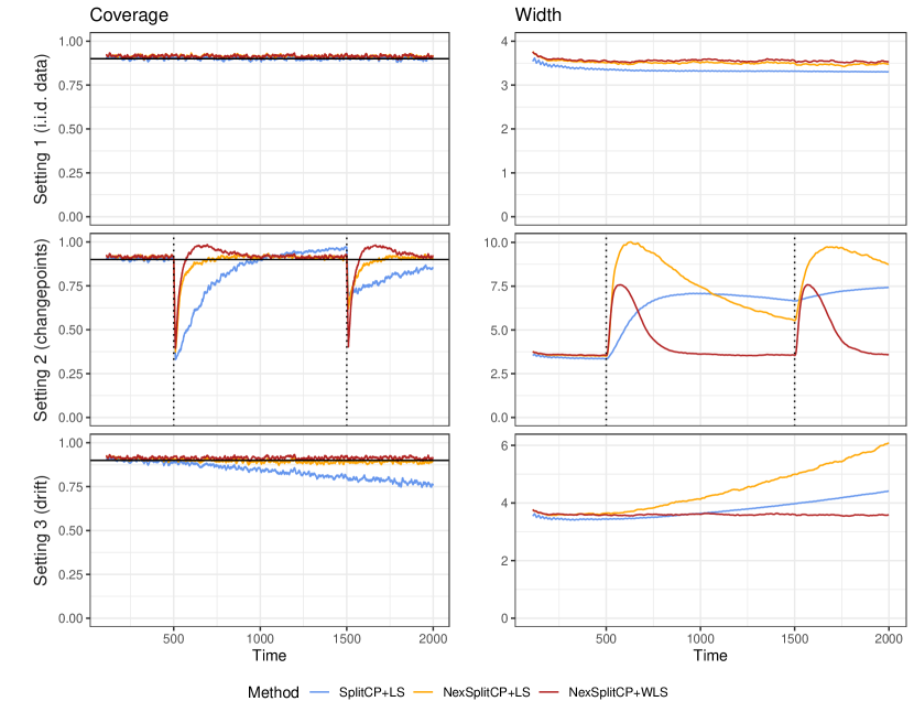
Figure 5: Simulation results showing mean prediction interval coverage and width for split conformal methods, averaged over 200 independent trials. The curves are smoothed by taking a rolling average with a window of 10 time points.

Figure 6: Simulation results showing mean prediction interval coverage and width for jacknife+ methods, averaged over 200 independent trials. The curves are smoothed by taking a rolling average with a window of 10 time points.

Appendix G Election data set description

To prepare the data, we followed the protocol from Gibbs and Candès [2021] and, therefore, quote from the above reference:

The county-level demographic characteristics used for prediction were the proportion of the total population that fell into each of the following race categories (either alone or in combination): black or African American, American Indian or Alaska Native, Asian, Native Hawaiian or other Pacific islander. In addition to this, we also used the proportion of the total population that was male, of Hispanic origin and that fell within each of the age ranges 20-29, 30-44, 45-64, and 65+. Demographic information was obtained from 2019 estimates published by the United States Census Bureau and available at [United States Census Bureau, 2019a]. In addition to these demographic features we also used the median household income and the percentage of individuals with a bachelors degree or higher as covariates. Data on county-level median household incomes was based on 2019 estimates obtained from [United States Census Bureau, 2019c]. The percentage of individuals with a bachelors degree or higher was computed based on data collected during the years 2015-2019 and published at [United States Census Bureau, 2019b]. As an aside, we remark that we used 2019 estimates because this was the most recent year for which data was available.

For 2016 covariate data, we used the same data sources, subject to the important distinction that we—almost exclusively—used published figures available by 2016. (The U.S. Census Bureau sometimes updates its figures so we cannot rule out the possibility that a few entries were changed post 2016.) Finally, vote counts for the 2016 election were obtained from MIT Election Data and Science Lab [2018], while 2020 election data was taken from Leip [2020]. In total, matching covariate and election vote count data were obtained for 3111 counties. Merging 2016 and 2020 data left us with 3076 counties (1119 in the training set and 1957 in the test set).

References

• Angelopoulos and Bates [2021] Anastasios N. Angelopoulos and Stephen Bates. A gentle introduction to conformal prediction and distribution-free uncertainty quantification. arXiv preprint arXiv:2107.07511, 2021.
• Barber et al. [2021] Rina Foygel Barber, Emmanuel J. Candès, Aaditya Ramdas, and Ryan J. Tibshirani. Predictive inference with the jackknife+. Annals of Statistics, 49(1):486–507, 2021.
• Bates et al. [2021] Stephen Bates, Emmanuel J. Candès, Lihua Lei, Yaniv Romano, and Matteo Sesia. Testing for outliers with conformal p-values. arXiv preprint arXiv:2104.08279, 2021.
• Burnaev and Vovk [2014] Evgeny Burnaev and Vladimir Vovk. Efficiency of conformalized ridge regression. In Conference on Learning Theory, pages 605–622, 2014.
• Candès et al. [2021] Emmanuel J. Candès, Lihua Lei, and Zhimei Ren. Conformalized survival analysis. arXiv preprint arXiv:2103.09763, 2021.
• Cauchois et al. [2020] Maxime Cauchois, Suyash Gupta, Alnur Ali, and John C. Duchi. Robust validation: Confident predictions even when distributions shift. arXiv preprint arXiv:2008.04267, 2020.
• Cherian and Bronner [2020] John Cherian and Leonard Bronner. How The Washington Post estimates outstanding votes for the 2020 presidential election, 2020. URL https://s3.us-east-1.amazonaws.com/elex-models-prod/2020-general/write-up/election_model_writeup.pdf.
• Chernozhukov et al. [2018] Victor Chernozhukov, Kaspar Wüthrich, and Zhu Yinchu. Exact and robust conformal inference methods for predictive machine learning with dependent data. In Conference On learning theory, pages 732–749. PMLR, 2018.
• Dunn et al. [2022] Robin Dunn, Larry Wasserman, and Aaditya Ramdas. Distribution-free prediction sets for two-layer hierarchical models. Journal of the American Statistical Association (to appear), 2022.
• Fannjiang et al. [2022] Clara Fannjiang, Stephen Bates, Anastasios N. Angelopoulos, Jennifer Listgarten, and Michael I. Jordan. Conformal prediction for the design problem. arXiv preprint arXiv:2202.03613, 2022.
• Gibbs and Candès [2021] Isaac Gibbs and Emmanuel J. Candès. Adaptive conformal inference under distribution shift. Advances in Neural Information Processing Systems, 34, 2021.
• Guan [2021] Leying Guan. Localized conformal prediction: A generalized inference framework for conformal prediction. arXiv preprint arXiv:2106.08460, 2021.
• Harries [1999] Michael Harries. Splice-2 comparative evaluation: Electricity pricing. Technical report, University of New South Wales, 1999.
• Harrison [2012] Matthew T. Harrison. Conservative hypothesis tests and confidence intervals using importance sampling. Biometrika, 99(1):57–69, 2012.
• Kivaranovic et al. [2020] Danijel Kivaranovic, Kory D. Johnson, and Hannes Leeb. Adaptive, distribution-free prediction intervals for deep networks. In International Conference on Artificial Intelligence and Statistics. PMLR, 2020.
• Landau [1953] Hyman G. Landau. On dominance relations and the structure of animal societies: III. The condition for a score structure. The Bulletin of Mathematical Biophysics, 15(2):143–148, 1953.
• Lei [2019] Jing Lei. Fast exact conformalization of the lasso using piecewise linear homotopy. Biometrika, 106(4):749–764, 2019.
• Lei and Wasserman [2014] Jing Lei and Larry Wasserman. Distribution-free prediction bands for non-parametric regression. Journal of the Royal Statistical Society: Series B, 76(1):71–96, 2014.
• Lei et al. [2013] Jing Lei, James Robins, and Larry Wasserman. Distribution-free prediction sets. Journal of the American Statistical Association, 108(501):278–287, 2013.
• Lei et al. [2018] Jing Lei, Max G’Sell, Alessandro Rinaldo, Ryan J. Tibshirani, and Larry Wasserman. Distribution-free predictive inference for regression. Journal of the American Statistical Association, 113(523):1094–1111, 2018.
• Lei and Candès [2021a] Lihua Lei and Emmanuel J. Candès. Conformal inference of counterfactuals and individual treatment effects. Journal of the Royal Statistical Society: Series B, 2021a.
• Lei and Candès [2021b] Lihua Lei and Emmanuel J. Candès. Theory of weighted conformal inference. Technical report, Stanford University, 2021b.
• Leip [2020] David Leip. Dave Leip’s atlas of U.S. presidential elections, 2020. URL http://uselectionatlas.org.
• Mao et al. [2020] Huiying Mao, Ryan Martin, and Brian Reich. Valid model-free spatial prediction. arXiv preprint arXiv:2006.15640, 2020.
• MIT Election Data and Science Lab [2018] MIT Election Data and Science Lab. County Presidential Election Returns 2000-2016, 2018. URL https://doi.org/10.7910/DVN/VOQCHQ.
• Podkopaev and Ramdas [2021] Aleksandr Podkopaev and Aaditya Ramdas. Distribution-free uncertainty quantification for classification under label shift. In Uncertainty in Artificial Intelligence. PMLR, 2021.
• Ramdas et al. [2019] Aaditya Ramdas, Rina Foygel Barber, Martin J. Wainwright, and Michael I. Jordan. A unified treatment of multiple testing with prior knowledge using the p-filter. Annals of Statistics, 47(5):2790–2821, 2019.
• Romano et al. [2019] Yaniv Romano, Evan Patterson, and Emmanuel J. Candès. Conformalized quantile regression. Advances in Neural Information Processing Systems, 32, 2019.
• Ross and Peköz [2007] Sheldon M. Ross and Erol A. Peköz. A Second Course in Probability. Probability Bookstore, 2007.
• Shafer and Vovk [2008] Glenn Shafer and Vladimir Vovk. A tutorial on conformal prediction. Journal of Machine Learning Research, 9(3), 2008.
• Stankeviciute et al. [2021] Kamile Stankeviciute, Ahmed M Alaa, and Mihaela van der Schaar. Conformal time-series forecasting. Advances in Neural Information Processing Systems, 34, 2021.
• Storey [2002] John D Storey. A direct approach to false discovery rates. Journal of the Royal Statistical Society: Series B, 64(3):479–498, 2002.
• Storey et al. [2004] John D. Storey, Jonathan E. Taylor, and David Siegmund. Strong control, conservative point estimation and simultaneous conservative consistency of false discovery rates: A unified approach. Journal of the Royal Statistical Society: Series B, 66(1):187–205, 2004.
• Tibshirani et al. [2019] Ryan J. Tibshirani, Rina Foygel Barber, Emmanuel J. Candès, and Aaditya Ramdas. Conformal prediction under covariate shift. Advances in Neural Information Processing Systems, 32, 2019.
• United States Census Bureau [2019a] United States Census Bureau. County characteristics resident population estimates, 2019a. Data retrieved from https://www.census.gov/data/tables/time-series/demo/popest/2010s-counties-detail.html.
• United States Census Bureau [2019b] United States Census Bureau. 2015-2019 american community survey 5-year average county-level estimates, 2019b. Data retrieved from https://www.ers.usda.gov/data-products/county-level-data-sets/download-data/.
• United States Census Bureau [2019c] United States Census Bureau. Small area income and poverty estimates: 2019, 2019c. Data retrieved from https://www.ers.usda.gov/data-products/county-level-data-sets/download-data/.
• Volkhonskiy et al. [2017] Denis Volkhonskiy, Evgeny Burnaev, Ilia Nouretdinov, Alexander Gammerman, and Vladimir Vovk. Inductive conformal martingales for change-point detection. In Conformal and Probabilistic Prediction and Applications, pages 132–153. PMLR, 2017.
• Vovk [2015] Vladimir Vovk. Cross-conformal predictors. Annals of Mathematics and Artificial Intelligence, 74(1):9–28, 2015.
• Vovk [2021] Vladimir Vovk. Testing randomness online. Statistical Science, 36(4):595–611, 2021.
• Vovk et al. [2005] Vladimir Vovk, Alex Gammerman, and Glenn Shafer. Algorithmic Learning in a Random World. Springer Science & Business Media, 2005.
• Vovk et al. [2018] Vladimir Vovk, Ilia Nouretdinov, Valery Manokhin, and Alexander Gammerman. Cross-conformal predictive distributions. In Conformal and Probabilistic Prediction and Applications, pages 37–51. PMLR, 2018.
• Vovk et al. [2021] Vladimir Vovk, Ivan Petej, and Alex Gammerman. Protected probabilistic classification. In Conformal and Probabilistic Prediction and Applications, pages 297–299. PMLR, 2021.
• Xu and Xie [2021] Chen Xu and Yao Xie. Conformal prediction interval for dynamic time-series. In International Conference on Machine Learning. PMLR, 2021.
• Zaffran et al. [2022] Margaux Zaffran, Olivier Féron, Yannig Goude, Julie Josse, and Aymeric Dieuleveut. Adaptive conformal predictions for time series. In International Conference on Machine Learning. PMLR, 2022.