Experimental study of turbulent thermal diffusion of particles in inhomogeneous and anisotropic turbulence

Abstract

We study experimentally turbulent thermal diffusion of small particles in inhomogeneous and anisotropic stably stratified turbulence produced by one oscillating grid in the air flow. The velocity fields have been measured using a Particle Image Velocimetry (PIV). We have determined various turbulence characteristics: the mean and turbulent velocities, two-point correlation functions of the velocity field and an integral scale of turbulence from the measured velocity fields. The temperature field have been measured with a temperature probe equipped with 12 E thermocouples. Spatial distributions of micron size particles have been determined by a PIV system using the effect of the Mie light scattering by particles in the flow. The experiments have demonstrated that particles are accumulated at the minimum of mean fluid temperature due to phenomenon of turbulent thermal diffusion. Using measured spatial distributions of particles and temperature fields, we have determined the effective turbulent thermal diffusion coefficient of particles in inhomogeneous temperature stratified turbulence. This experimental study has clearly detected phenomenon of turbulent thermal diffusion in inhomogeneous turbulence.

I Introduction

Turbulent transport and mixing of aerosols and droplets is of fundamental importance in a large variety of applications ranging from environmental sciences, physics of the atmosphere and meteorology to industrial turbulent flows and turbulent combustion [1, 2, 3, 4, 5, 6, 7]. Various laboratory experiments and numerical simulations as well as observations in atmospheric and astrophysical turbulence have detected large-scale long-living clusters of particles as well as small-scale particle clusters [4, 5, 6, 7, 8, 9, 10, 11, 12]. Characteristic scales of large-scale clusters are much larger than the integral turbulence scale, while characteristic scales of small-scale clusters are much smaller than the integral turbulence scale.

Turbulent diffusion causes a decay of inhomogeneous particle clusters. On the other hand, turbulence can create inhomogeneous particle spatial distributions. For instance, small-scale clusters are formed in non-stratified [13, 18, 14, 15, 16, 17] and stratified turbulence [18, 19, 20]. The large-scale clusters of inertial particles in isothermal non-stratified inhomogeneous turbulence are caused by turbophoresis [21, 22, 23, 24, 11, 25], which is a combined effect of particle inertia and inhomogeneity of turbulence.

The large-scale clusters in a temperature-stratified turbulence are formed due to turbulent thermal diffusion [26, 27], resulting in additional turbulent non-diffusive flux of particles directed to the minimum of the mean temperature. The characteristic spatial scale of particle clusters formed due to turbulent thermal diffusion is much larger than the integral scale of turbulence, and the characteristic time scale of the formation of the particle clusters is much larger than the characteristic turbulent time scale. Turbulent thermal diffusion is a purely collective phenomenon resulting in a pumping effect, described in terms of effective velocity of particles in the direction opposite to the mean temperature gradient. A balance between the turbulent thermal diffusion and turbulent diffusion determines the conditions for the formation of large-scale particle clusters.

Turbulent thermal diffusion has been studied theoretically [26, 27, 28, 29, 30, 31, 32, 33] and detected in different laboratory experiments in stably and convective temperature-stratified turbulence produced by oscillating grids [34, 35, 36] or a multi-fan generator [37]. This phenomenon has been also detected in direct numerical simulations [38, 39]. Turbulent thermal diffusion is shown to be a crucial importance in the atmospheric turbulence with temperature inversions [40] and in astrophysical temperature stratified turbulent flows [41]. Turbulent thermal diffusion plays an important role in formation of small-scale particle clusters in turbulence with a mean vertical temperature gradient [19, 20].

Turbulent thermal diffusion of small particles has been investigated mainly in a homogeneous turbulence produced by two oscillating grids [34, 35, 36, 37]. In the present experimental study we investigate phenomenon of turbulent thermal diffusion of small particles in inhomogeneous and anisotropic stably stratified turbulence produced by one oscillating grid in the air flow. Previous experiments [42, 43, 44, 45, 46, 47, 48] with one oscillating grid have been performed in a water flow with isothermal turbulence. It has been shown in these experiments that the integral scale $\ell_{0}$ of turbulence is proportional to the distance $Y$ from a grid ($\ell_{0}\propto Y$), and the root mean square (r.m.s.) velocity scales as $\sqrt{\langle{\bf u^{\prime}}^{2}\rangle}\propto f\,Y^{-1}$, where $f$ is the frequency of the grid oscillations. This implies that Reynolds numbers and the turbulent diffusion coefficient in the core flow of inhomogeneous turbulence are weakly dependent on the distance from the grid.

In this paper we discuss the results of experimental study of turbulent transport of small particles in inhomogeneous stably stratified turbulence in the air flow with an imposed temperature gradient. This paper is organized as follows. In Section II we discuss physics of the phenomenon of turbulent thermal diffusion. In Section  III we describe the experimental setup and measurements techniques. In Section  IV we discuss the experimental results of particle transport in inhomogeneous and anisotropic stably stratified turbulence produced by one oscillating grid. In this section we determine spatial distributions of turbulence parameters and find spatial distributions of the mean fluid temperature and the mean number density of particles. This allows us to determine the characteristics of turbulent thermal diffusion of particles in inhomogeneous turbulence. Finally, conclusions are drawn in Section V.

II Physics of turbulent thermal diffusion

In this section we discuss the physics of phenomenon of turbulent thermal diffusion. First, we consider dynamics of small non-inertial particles or gaseous admixtures in a turbulent fluid flow. Equation for the evolution of the particle number density $n(t,{\bm{x}})$ in a compressible fluid velocity field ${\bm{U}}(t,{\bm{x}})$ reads [49, 50]

$${\partial n\over\partial t}+{\bm{\nabla}}{\bf\cdot}({\bm{U}}\,n)=D\,\Delta n,$$ (1)

where $D=k_{B}\,T/(3\pi\rho\,\nu\,d_{\rm p})$ is the coefficient of the molecular (Brownian) diffusion of particles, $d_{\rm p}$ is the particle diameter, $\nu$ is the kinematic viscosity of the fluid, $T$ and $\rho$ are the fluid temperature and density and $k_{B}$ is the Boltzmann constant. We consider fluid flows with a low Mach number, Ma $=|{\bm{U}}|/c_{\rm s}\ll 1$, which implies that fluid velocity is much less than the sound speed, $c_{\rm s}$. In this case the continuity equation for the fluid density can be used in an anelastic approximation, $\mbox{\boldmath$\nabla$}{\bf\cdot}(\rho\,{\bm{U}})=0$, which takes into account an inhomogeneous distribution of the fluid density.

We study a long-term evolution of the particle number density in spatial scales $L_{n}$ which are much larger than the integral scale of turbulence $\ell_{0}$, and during the time scales $t_{n}$ which are much larger than the turbulent time scales $\tau_{0}$. We use a mean-field approach, where all quantities are decomposed into the mean and fluctuating parts, and the fluctuating parts have zero mean values, i.e., we use the Reynolds averaging. In particular, the particle number density $n=\overline{n}+n^{\prime}$, where $\overline{n}=\langle n\rangle$ is the mean particle number density, $n^{\prime}$ are particle number density fluctuations and $\langle n^{\prime}\rangle=0$. The angular brackets denote ensemble averaging. Averaging Eq. (1) over an ensemble of turbulent velocity field, we arrive at the mean-field equation for the particle number density:

$${\partial\overline{n}\over\partial t}+{\bm{\nabla}}{\bf\cdot}\langle{\bm{u}}\,n^{\prime}\rangle=D\,\Delta\overline{n},$$ (2)

where $\langle{\bm{u}}\,n^{\prime}\rangle$ is the turbulent flux of particles and ${\bm{u}}$ are velocity fluctuations. Here we consider for simplicity the case when the mean velocity vanishes, i.e., $\overline{\bm{U}}=0$.

Equation (2) is not yet closed because we do not know how the particle turbulent flux $\langle{\bm{u}}n^{\prime}\rangle$ depends on the mean particle number density $\overline{n}$. To determine the particle turbulent flux, we derive an equation for particle number density fluctuations $n^{\prime}$, that is obtained by subtracting Eq. (2) from Eq. (1):

$${\partial n^{\prime}\over\partial t}+{\bm{\nabla}}{\bf\cdot}\left(n^{\prime}{\bm{u}}-\langle n^{\prime}{\bm{u}}\rangle\right)-D\Delta n^{\prime}=-({\bm{u}}{\bf\cdot}{\bm{\nabla}})\overline{n}-\overline{n}({\bm{\nabla}}{\bf\cdot}{\bm{u}}).$$

(3)

The term, ${\cal Q}={\bm{\nabla}}{\bf\cdot}\left(n^{\prime}\,{\bm{u}}-\langle n^{\prime}\,{\bm{u}}\rangle\right)$, in the left-hand side of Eq. (3) is the nonlinear term, while the terms, $-({\bm{u}}{\bf\cdot}{\bm{\nabla}})\overline{n}-\overline{n}({\bm{\nabla}}{\bf\cdot}{\bm{u}})$, in the right-hand side of Eq. (3) are the source terms for particle number density fluctuations. The first source term, $-({\bm{u}}{\bf\cdot}\mbox{\boldmath$\nabla$})\overline{n}$, in Eq. (3) causes production of particle number density fluctuations by the tangling of the gradient of the mean particle number density ${\bm{\nabla}}\,\overline{n}$ by velocity fluctuations.

The second source term in Eq. (3) is $-\overline{n}({\bm{\nabla}}{\bf\cdot}{\bm{u}})$. Let us decompose the fluid density into the mean fluid density $\overline{\rho}$ and fluctuations $\rho^{\prime}$, i.e., $\rho=\overline{\rho}+\rho^{\prime}$, where for low Mach numbers $|\rho^{\prime}|\ll\overline{\rho}$. The anelastic approximation yields $\mbox{\boldmath$\nabla$}{\bf\cdot}(\rho\,{\bm{u}})\approx\mbox{\boldmath$\nabla$}{\bf\cdot}(\overline{\rho}\,{\bm{u}})=0$, so that $\mbox{\boldmath$\nabla$}{\bf\cdot}{\bm{u}}\approx-({\bm{u}}\cdot{\bm{\nabla}})\,\overline{\rho}/\overline{\rho}$. Introducing a vector ${\bm{\lambda}}=-{\bm{\nabla}}\overline{\rho}/\overline{\rho}$, we obtain that $\mbox{\boldmath$\nabla$}{\bf\cdot}{\bm{u}}\approx{\bm{u}}\cdot{\bm{\lambda}}$. Thus, the second source term, $-\overline{n}({\bm{\nabla}}{\bf\cdot}{\bm{u}})=(\overline{n}/\overline{\rho}\,)({\bm{u}}{\bf\cdot}{\bm{\nabla}})\overline{\rho}=-\overline{n}\,({\bm{u}}{\bf\cdot}{\bm{\lambda}})$, causes production of particle number density fluctuations by the tangling of the gradient of the mean fluid density ${\bm{\nabla}}\,\overline{\rho}\,$ by velocity fluctuations. The ratio of the absolute values of the nonlinear term $|{\cal Q}|$ to the diffusion term $|D\Delta n^{\prime}|$ is the Péclet number for particles, that can be estimated as ${\rm Pe}=u_{0}\,\ell_{0}/D$.

Equation (3) is a nonlinear equation for particle number density fluctuations. Since this nonlinear equation cannot be solved exactly for arbitrary Péclet numbers, one has to use different approximate methods for the solution of Eq. (3). We consider a one-way coupling, i.e., we take into account the effect of the turbulent velocity on the particle number density, but we neglect the feedback effect of the particle number density on the turbulent fluid flow. This approximation is valid when the spatial density of particles $n\,m_{p}$ is much smaller than the fluid density $\rho$, where $m_{p}$ is the particle mass. We also consider non-inertial particles or gaseous admixtures. In this case the particles move with the fluid velocity. These assumptions imply that the particle number density is a passive scalar.

We use for simplicity the dimensional analysis to solve Eq. (3). The dimension of the left-hand side of Eq. (3) is the rate of change of particle number density fluctuations $n^{\prime}/\tau_{n^{\prime}}$, where $\tau_{n^{\prime}}$ is the characteristic time of particle number density fluctuations. For large Reynolds and Péclet numbers, the characteristic time of particle number density fluctuations $\tau_{n^{\prime}}$ can be identified with the correlation time $\tau_{0}$ of the turbulent velocity field. Therefore, in the framework of the dimensional analysis, we replace the left-hand side of Eq. (3) by $n^{\prime}/\tau_{0}$. This yields:

$$n^{\prime}=-\tau_{0}\,\left[({\bm{u}}{\bf\cdot}{\bm{\nabla}})\overline{n}+\overline{n}\,({\bm{\nabla}}{\bf\cdot}{\bm{u}})\right].$$ (4)

Multiplying Eq. (4) by velocity fluctuations, $u_{i}$, and averaging over an ensemble of turbulent velocity field, we arrive at the expression for the turbulent flux of particles:

$$\left\langle n^{\prime}\,u_{i}\right\rangle = -\tau_{0}\,\left\langle u_{i}u_{j}\right\rangle\,\nabla_{j}\overline{n}-\tau_{0}\,\overline{n}\,\left\langle u_{i}(\mbox{\boldmath$\nabla$}{\bf\cdot}{\bm{u}})\right\rangle$$ (5)

$$\equiv V_{i}^{\rm eff}\,\overline{n}-D_{ij}^{(n)}\,\nabla_{j}\overline{n},$$

where the last term, $-D_{ij}^{(n)}\,\nabla_{j}\overline{n}$, in Eq. (5) determines the contribution to the flux of particles caused by turbulent diffusion, and $D_{ij}^{(n)}=\tau_{0}\,\left\langle u_{i}u_{j}\right\rangle$ is the turbulent diffusion tensor. For an isotropic turbulence $\langle u_{i}u_{j}\rangle=\delta_{ij}\,\langle{\bm{u}}^{2}\rangle/3$, so that the turbulent diffusion tensor for large Péclet numbers is given by $D_{ij}^{(n)}=D_{\rm T}\delta_{ij}$, where $D_{\rm T}=\tau_{0}\,\left\langle{\bm{u}}^{2}\right\rangle/3$ is the turbulent diffusion coefficient.

The term ${\bm{V}}^{\rm eff}\,\overline{n}$ in Eq. (5) determines the contribution to the turbulent flux of particles caused by the effective pumping velocity: ${\bm{V}}^{\rm eff}=-\tau_{0}\,\left\langle{\bm{u}}(\mbox{\boldmath$\nabla$}{\bf\cdot}{\bm{u}})\right\rangle$. Next, we take into account the anelastic approximation, ${\bm{\nabla}}{\bf\cdot}{\bm{u}}=-(1/\overline{\rho})\,({\bm{u}}{\bf\cdot}{\bm{\nabla}})\overline{\rho}$, so that the effective pumping velocity is given by $V_{i}^{\rm eff}=-\tau_{0}\,\left\langle u_{i}u_{j}\right\rangle\,\lambda_{j}$, where ${\bm{\lambda}}=-{\bm{\nabla}}\overline{\rho}/\overline{\rho}$. For an isotropic turbulence, the effective pumping velocity is given by [26, 27]

$${\bm{V}}^{\rm eff}=D_{\rm T}\,{{\bm{\nabla}}\overline{\rho}\over\overline{\rho}},$$ (6)

and the particle turbulent flux $\langle{\bm{u}}\,n^{\prime}\rangle$ is

$$\left\langle{\bm{u}}\,n^{\prime}\right\rangle={\bm{V}}^{\rm eff}\,\overline{n}-D_{\rm T}\,{\bm{\nabla}}\overline{n}.$$ (7)

To understand the physics related to the effective pumping velocity ${\bm{V}}^{\rm eff}$, let us first express the effective pumping velocity via physical parameters. We use the equation of state for a perfect gas, $P=(k_{B}/m_{\mu})\,\rho\,T$, that can be also rewritten for the mean fields as $\overline{P}=(k_{B}/m_{\mu})\,\overline{\rho}\,\overline{T}$, where $\overline{P}$ and $\overline{T}$ are the mean pressure and mean temperature, respectively. Here we assume that $\overline{\rho}\,\overline{T}\gg\langle\rho^{\prime}\,\theta\rangle$. By means of the equation of state, we express the gradient of the mean fluid density in terms of the gradients of the mean fluid pressure ${\bm{\nabla}}\overline{P}$ and mean fluid temperature ${\bm{\nabla}}\overline{T}$ as ${\bm{\nabla}}\,\ln\overline{\rho}={\bm{\nabla}}\ln\overline{P}-{\bm{\nabla}}\ln\overline{T}$. For small mean pressure gradient, ${\bm{\nabla}}\,\ln\overline{\rho}\approx-{\bm{\nabla}}\overline{T}$, so that the effective pumping velocity of non-inertial particles is given by [26, 27]

$${\bm{V}}^{\rm eff}=-D_{\rm T}\,{{\bm{\nabla}}\overline{T}\over\overline{T}}.$$ (8)

The rigorous methods yield the result similar to Eq. (8) (see, e.g., [7]). For inertial particles, the effective pumping velocity is given by

$${\bm{V}}^{\rm eff}=-\alpha\left(d_{\rm p},{\rm Re}\right)\,D_{\rm T}\,{{\bm{\nabla}}\overline{T}\over\overline{T}},$$ (9)

where the effective turbulent thermal diffusion coefficient of particles is

$$\alpha(d_{\rm p},{\rm Re})=1+{\tau_{p}(d_{\rm p})\over\tau_{0}}\,{\rm Re}^{1/4}\,\ln({\rm Re})\,\left({L_{\rm eff}\over\ell_{0}}\right),$$

(10)

(see [24, 28, 20, 33]). Here $L_{\rm eff}=2c_{s}^{2}\tau_{\eta}^{3/2}/3\nu^{1/2}$ is the effective length scale, $c_{s}$ is the sound speed, $\tau_{\rm p}=m_{\rm p}/(3\pi\rho\,\nu d_{\rm p})$ is the Stokes time for particles having mass $m_{\rm p}$ and diameter $d_{\rm p}$, $\tau_{\eta}=\tau_{0}/\sqrt{\rm Re}$ is the Kolmogorov viscous time, ${\rm Re}=\tau_{0}\langle{\bm{u}}^{2}\rangle/\nu$ is the Reynolds number and $\nu$ is the kinematic viscosity. For the conditions pertinent to our laboratory experiments, the function $\alpha$ varies for the micron-size particles from 2 to 3 depending on Reynolds number.

Substituting Eq. (7) into Eq. (2), we arrive at the evolutionary equation for the particle mean number density as

$${\partial\overline{n}\over\partial t}+\nabla_{z}\left[V_{z}^{\rm(eff)}\,\overline{n}-\left(D+D_{\rm T}\right)\,\nabla_{z}\overline{n}\right]=0.$$ (11)

The steady-state solution of Eq. (11) for the mean number density of particles with a zero total flux of particles at the vertical boundaries is given by

$${\overline{n}(z)\over\overline{n}_{0}}=\left({\overline{T}(z)\over\overline{T}_{0}}\right)^{-{\alpha D_{\rm T}\over D_{\rm T}+D}},$$ (12)

where $\overline{T}_{0}$ and $\overline{n}_{0}$ are the values of the mean fluid temperature and the particle mean number density at the vertical boundaries. Here we take into account Eq. (9). It follows from Eq. (12), that particles are accumulated at the vicinity of the minimum of the mean temperature.

The physics of the effect of turbulent thermal diffusion for solid particles is as follows [26, 27]. The inertia causes particles inside the turbulent eddies to drift out to the boundary regions between eddies due to the centrifugal inertial force, so that inertial particles are locally accumulated in these regions. These regions have low vorticity fluctuations, high strain rate and high pressure fluctuations [51]. Similarly, there is an outflow of inertial particles from regions with minimum fluid pressure fluctuations. In homogeneous and isotropic turbulence with a zero gradient of the mean temperature, there is no preferential direction, so that there is no large-scale effect of particle accumulation.

In temperature-stratified turbulence, fluctuations of fluid temperature $\theta$ and velocity ${\bm{u}}$ are correlated due to a non-zero turbulent heat flux, $\langle\theta\,{\bm{u}}\rangle\not=\bm{0}$. Fluctuations of temperature cause pressure fluctuations, which result in fluctuations of the number density of particles. In the mechanism of turbulent thermal diffusion, only pressure fluctuations which are correlated with velocity fluctuations due to a non-zero turbulent heat flux play a crucial role. Increase of the fluid pressure fluctuations is accompanied by an accumulation of particles, and the direction of the mean flux of particles coincides with that of the turbulent heat flux. The turbulent flux of particles is directed to the minimum of the mean temperature, and the particles tend to be accumulated in this region [7].

The similar effect of accumulation of particles in the vicinity of the mean temperature minimum (or in the vicinity of the maximum of the mean fluid density) and the formation of inhomogeneous spatial distributions of the mean particle number density exists also for non-inertial particles or gaseous admixtures in density-stratified or temperature-stratified turbulence, i.e., for a low-Mach-number compressible turbulent fluid flow [27, 38, 39].

The physics of the accumulation of non-inertial particles in the vicinity of the maximum of the mean fluid density can be explained as follows. Let us assume that the mean fluid density $\overline{\rho}_{2}$ at point $2$ is larger than the mean fluid density $\overline{\rho}_{1}$ at point $1$. Consider two small control volumes a and b located between these two points, and let the direction of the local turbulent velocity in volume a at some instant be the same as the direction of the mean fluid density gradient $\mbox{\boldmath$\nabla$}\,\overline{\rho}$ (i.e., along the $x$ axis toward point $2$). Let the local turbulent velocity in volume b at this instant be directed opposite to the mean fluid density gradient (i.e., toward point $1$).

In a fluid flow with a nonzero mean fluid density gradient, one of the sources of particle number density fluctuations, $n^{\prime}\propto-\tau_{0}\,\overline{n}\,(\mbox{\boldmath$\nabla$}{\bf\cdot}\,{\bm{u}})$, is caused by a non-zero $\mbox{\boldmath$\nabla$}\cdot{\bm{u}}\approx-{\bm{u}}\cdot\mbox{\boldmath$\nabla$}\ln\overline{\rho}\not=0$. Since fluctuations of the fluid velocity ${\bm{u}}$ are positive in volume a and negative in volume b, we have the negative divergence of the fluid velocity, $\mbox{\boldmath$\nabla$}{\bf\cdot}\,{\bm{u}}<0$, in volume a, and the positive divergence of the fluid velocity, $\mbox{\boldmath$\nabla$}{\bf\cdot}\,{\bm{u}}>0$, in volume b. Therefore, fluctuations of the particle number density $n^{\prime}\propto-\tau_{0}\,\overline{n}\,(\mbox{\boldmath$\nabla$}{\bf\cdot}\,{\bm{u}})$ are positive in volume a and negative in volume b. However, the flux of particles $n^{\prime}\,u_{x}$ is positive in volume a (i.e., it is directed toward point $2$), and it is also positive in volume b (because both fluctuations of fluid velocity and number density of particles are negative in volume b). Therefore, the mean flux of particles $\langle n^{\prime}{\bm{u}}\rangle$ is directed, as is the mean fluid density gradient $\mbox{\boldmath$\nabla$}\,\overline{\rho}$, toward point 2. This results in formation large-scale heterogeneous structures of non-inertial particles in regions with a mean fluid density maximum. When the gradient $\mbox{\boldmath$\nabla$}\,\overline{P}$ of the mean fluid pressure vanishes, $(\mbox{\boldmath$\nabla$}\,\overline{\rho})/\overline{\rho}=-(\mbox{\boldmath$\nabla$}\,\overline{T})/\overline{T}$. This implies that particles are accumulated at the vicinity of the minimum of the fluid temperature [27, 7].

Compressibility in a low-Mach-number stratified turbulent fluid flow causes an additional non-diffusive component of the turbulent flux of non-inertial particles or gases, and results in the formation of large-scale inhomogeneous structures in spatial distributions of non-inertial particles. In a temperature stratified turbulence, preferential concentration of particles caused by turbulent thermal diffusion can occur in the vicinity of the minimum of the mean temperature.

III Experimental setup

In the present paper we study turbulent thermal diffusion of small particles in experiments with inhomogeneous and anisotropic stably stratified turbulence produced by one oscillating grid in the air flow. In this section we describe very briefly the experimental set-up and measurement facilities in the oscillating grid turbulence. The experiments in stably stratified turbulence have been conducted in rectangular chamber. The dimensions of the chamber are $L_{x}\times L_{y}\times L_{z}$, where $L_{x}=L_{z}=26$ cm, $L_{y}=53$ cm. The axis $Z$ is in the vertical direction and the axis $Y$ is perpendicular to the grid plain, so that the distance from the grid is measured along the $Y$ axis. Turbulence in a transparent chamber is produced by one oscillating vertically oriented grid with bars arranged in a square array. The grid is parallel to the side walls and positioned at a distance of two grid meshes from the chamber left wall (see Fig.  1). The grid is operated at the frequency $10.5$ Hz. The chosen frequency applied to the grid is the maximum possible frequency in our experimental setup before the grid can be damaged. It allows us to produce turbulence with the maximum intensity.

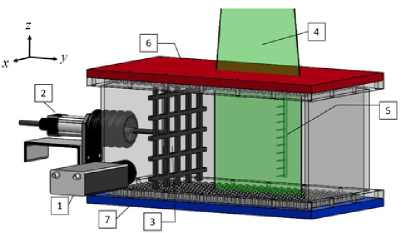
Figure 1: Experimental setup: (1) digital CCD camera; (2) rod driven by the speed-controlled motor; (3) oscillating grid; (4) laser light sheet; (5) temperature probe equipped with 12 E - thermocouples; (6) heat exchanger at the top cooled wall of the chamber; (7) heat exchanger at the bottom heated wall of the chamber.

A vertical mean temperature gradient in the turbulent air flow is formed by attaching two aluminium heat exchangers to the bottom (cooled) and top (heated) walls of the chamber which allow us to form a mean temperature gradient in a turbulent flow. To improve the heat transfer in the boundary layers at the bottom and top walls of the chamber, we use the heat exchangers with rectangular pins $3\times 3\times 15$ mm. This allows us to support a large mean temperature gradient in the core of the flow.

The temperature field is measured with a temperature probe equipped with 12 E - thermocouples (with the diameter of 0.13 mm and the sensitivity of $\approx 75\,\mu$V/K) attached to a vertical rod with a diameter 4 mm. The mean spacing between thermal couples along the rod is about 21.6 mm. Each thermocouple is inserted into a 1.15 mm diameter and 36 mm long case. A tip of a thermocouple protruded at the length of 8 mm out of the case.

The temperature is measured for 12 rod positions with 20 mm intervals in the horizontal direction. A sequence of 530 temperature readings for every thermocouple at every rod position is recorded and processed using the developed software based on LabView 7.0. Temperature maps are obtained using Matlab 9.7.0. A large mean temperature gradient up to 1.2 K/cm in the core flow and 3 K/cm close to the walls at a mean temperature of about 310 K can be formed.

The velocity field is measured using a Particle Image Velocimetry (PIV) [52, 53, 54]. In the experiments we use LaVision Flow Master III system. A double-pulsed light sheet is provided by a Nd-YAG laser (Continuum Surelite $2\times 170$ mJ). The light sheet optics includes spherical and cylindrical Galilei telescopes with tuneable divergence and adjustable focus length. We use a progressive-scan 12 bit digital CCD camera (with pixel size $6.45\,\mu$m $\times\,6.45\,\mu$m and $1376\times 1040$ pixels) with a dual-frame-technique for cross-correlation processing of captured images. A programmable Timing Unit (PC interface card) generate sequences of pulses to control the laser, camera and data acquisition rate. The software package LaVision DaVis 8.3 is applied to control all hardware components and for 32 bit image acquisition and visualization. This software package comprises PIV software for calculating the flow fields using cross-correlation analysis.

An incense smoke with sub-micron particles ($\rho_{\rm p}/\rho\sim 10^{3})$, is used as a tracer for the PIV measurements, where $\rho_{\rm p}$ is the material density of particles. Smoke is produced by high temperature sublimation of solid incense grains. Analysis of smoke particles using a microscope (Nikon, Epiphot with an amplification of 560) and a PM-300 portable laser particulate analyzer shows that these particles have an approximately spherical shape and that their mean diameter is of the order of $0.7\mu$m. The probability density function of the particle size measured with the PM-300 particulate analyzer is independent of the location in the flow for incense particle size of $0.5-1\,\mu$m. The maximum tracer particle displacement in the experiment is of the order of $1/4$ of the interrogation window. The average displacement of tracer particles is of the order of $1.5$ pixels. The average accuracy of the velocity measurements is of the order of $4\%$ for the accuracy of the correlation peak detection in the interrogation window of the order of $0.1$ pixel [52, 53, 54].

We have determined the following turbulence characteristics in the experiments: the mean and the root mean square (r.m.s.) velocities, two-point correlation functions and an integral scale of turbulence from the measured velocity fields. Series of 530 pairs of images acquired with a frequency of 4 Hz, are stored for calculating velocity maps and for ensemble and spatial averaging of turbulence characteristics. We measure velocity in a flow domain $197.12\times 157.7$ mm² with a spatial resolution of $1280\times 1024$ pixels. This corresponds to a spatial resolution 154 $\mu$m / pixel. The velocity field in the probed region is analyzed with interrogation windows of $32\times 32$ pixels. In every interrogation window a velocity vector is determined from which velocity maps comprising $80\times 64$ vectors are constructed. The mean and r.m.s. velocities for every point of a velocity map are calculated by averaging over 530 independent maps.

The two-point correlation functions of the velocity field are determined for every point of the velocity map (with $80\times 64$ vectors) by averaging over 530 independent velocity maps. The integral scales of turbulence $\ell_{y}$ and $\ell_{z}$ are determined in the horizontal $Y$ and the vertical $Z$ directions from the two-point correlation functions of the velocity field.

Particle spatial distribution is determined using PIV system. In particular, the effect of the Mie light scattering by particles was used to determine the particle spatial distribution in the flow [55]. The mean intensity of scattered light was determined in $40\times 32$ interrogation windows with the size $32\times 32$ pixels. The vertical distribution of the intensity of the scattered light was determined in 40 vertical strips composed of 32 interrogation windows.

The light radiation energy flux scattered by small particles is $E_{s}\propto E_{0}\Psi(\pi d_{\rm p}/\lambda;a_{0};n)$, where $E_{0}\propto\pi d_{\rm p}^{2}/4$ is the energy flux incident at the particle, $d_{\rm p}$ is the particle diameter, $\lambda$ is the wavelength, $a_{0}$ is the index of refraction and $\Psi$ is the scattering function. For wavelengths $\lambda$ which are larger than the particle perimeter $(\lambda>\pi d_{\rm p})$, the function $\Psi$ is given by Rayleigh’s law, $\Psi\propto d_{\rm p}^{4}$. If the wavelength is small, the function $\Psi$ tends to be independent of $d_{\rm p}$ and $\lambda$. In the general case the function $\Psi$ is given by the Mie equations [56].

The scattered light energy flux incident on the CCD camera probe (producing proportional charge in every CCD pixel) is proportional to the particle number density $n$, i.e., $E_{s}\propto E_{0}\,n\,(\pi d_{\rm p}^{2}/4)$. The probability density function of the particle size (measured with the PM300 particulate analyzer) was independent of the location in the flow. Indeed, since the number density of particles is small, so that they are about $1$ mm apart, it can be safely assumed that a change in particle number density $n$ does not affect their size distribution. Consequently, the ratio of the scattered radiation fluxes at two locations in the flow and at the image measured with the charge-coupled device (CCD) camera is equal to the ratio of the particle number densities at these two locations. Measurements performed using different concentration of the incense smoke showed that the distribution of the average scattered light intensity over a vertical coordinate was independent of the particle number density in the isothermal flow.

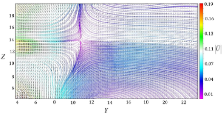
Figure 2: Mean velocity field in the core flow for isothermal turbulence. The velocity is measured in m/s and coordinates are in cm.

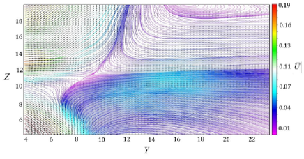
Figure 3: Mean velocity field in the core flow for temperature stratified turbulence. The velocity is measured in m/s and coordinates are in cm.

To characterize the spatial distribution of particle number density $n\propto E^{T}/E$ in the non-isothermal flow, the distribution of the scattered light intensity E measured in the isothermal case was used for the normalization of the scattered light intensity $E^{T}$ obtained in a non-isothermal flow under the same conditions. The scattered light intensities $E^{T}$ and $E$ in each experiment were normalized by corresponding scattered light intensities averaged over the vertical coordinate. The Mie scattering is not affected by temperature change because it depends on the electric permittivity of particles, the particle size and the laser light wave length. The temperature effect on these characteristics is negligibly small.

Similar experimental set-up and data processing procedure have been previously used by us in the experimental study of different aspects of turbulent convection [37, 57, 58], stably stratified turbulence [59], phenomenon of turbulent thermal diffusion in homogeneous turbulence [34, 35, 36, 37, 33] and small-scale particle clustering [19].

IV Experimental results

In this section we describe the obtained experimental results. The experiments for the temperature difference $\Delta T=50$ K between the top and bottom walls have been performed in the present study. From the measured velocity fields, we determine various turbulence characteristics for isothermal and stably stratified turbulence in horizontal and vertical directions: the mean velocity patterns, the turbulent velocity distributions, the two-point correlation functions of the velocity field which allow us to find the integral scales of turbulence.

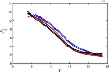
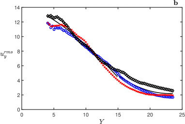
Figure 4: Horizontal component of the turbulent velocity $u^{\rm(rms)}_{y}$ versus $Y$ averaged over different vertical regions: $Z=6.5-11$ cm (black, diamonds); $Z=11-15$ cm (red, slanting crosses); $Z=15.2-18$ cm (blue, circles) for (a) isothermal turbulence (upper panel); fitting: $u^{\rm(rms)}_{y}=-0.05Y^{1.8}+12$ (solid) from $Y=4$ cm to 15 cm and $u^{\rm(rms)}_{y}=10^{5}Y^{-4}+1$ (solid) from $Y=15$ cm to 23.7 cm; and (b) temperature stratified turbulence (lower panel); fitting: $u^{\rm(rms)}_{y}=-0.17Y^{1.496}+14.15$ (solid) from $Y=4$ cm to 15 cm, $u^{\rm(rms)}_{y}=0.038\,Y^{-1.786}+22.73$ (solid) from $Y=15$ cm to 23.7 cm. The velocity is measured in cm/s and coordinates are in cm.

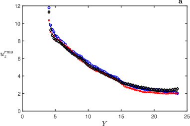
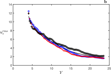
Figure 5: Vertical component of the turbulent velocity $u^{\rm(rms)}_{z}$ versus $Y$ averaged over different vertical regions: $Z=6.5-11$ cm (black, diamonds); $Z=11-15$ cm (red, slanting crosses); $Z=15.2-18$ cm (blue, circles) for (a) isothermal turbulence (upper panel); fitting: $u^{\rm(rms)}_{z}=33.58Y^{-1}+2$ (solid) from $Y=4$ cm to 10 cm, and $u^{\rm(rms)}_{z}=0.02Y^{2}-0.95Y+12.7$ (solid) from $Y=10$ cm to 23.7 cm; and (b) temperature stratified turbulence (lower panel); fitting: $u^{\rm(rms)}_{z}=42.8Y^{-1}+1$ (solid) from $Y=4$ cm to 11.5 cm; and $u^{\rm(rms)}_{z}=213Y^{-1.6}+0.36$ (solid) from $Y=11.5$ cm to 23.7 cm. The velocity is measured in cm/s and coordinates are in cm.

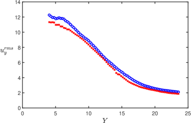
Figure 6: Horizontal component of the turbulent velocity $u^{\rm(rms)}_{y}$ versus $Y$ averaged over $Z$ for isothermal turbulence (red) and temperature stratified turbulence (blue). The velocity is measured in cm/s and coordinates are in cm.

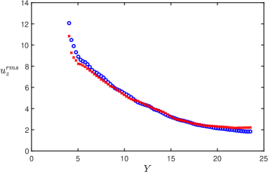
Figure 7: Horizontal component of the turbulent velocity $u^{\rm(rms)}_{z}$ versus $Y$ averaged over $Z$ for isothermal turbulence (red) and temperature stratified turbulence (blue). The velocity is measured in cm/s and coordinates are in cm.

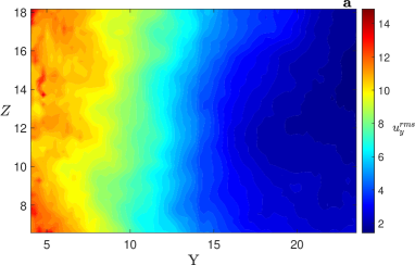
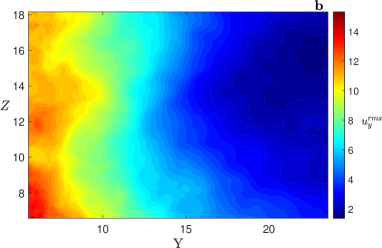
Figure 8: Counter lines of the horizontal component of the turbulent velocity $u^{\rm(rms)}_{y}$ for (a) isothermal turbulence (upper panel) and (b) temperature stratified turbulence (lower panel) in the $YZ$ plane. The velocity is measured in cm/s and coordinates are in cm.

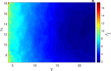
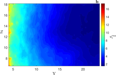
Figure 9: Counter lines for the vertical component of the turbulent velocity $u^{\rm(rms)}_{z}$ for (a) isothermal turbulence (upper panel) and (b) temperature stratified turbulence (lower panel) in the $YZ$ plane. The velocity is measured in cm/s and coordinates are in cm.

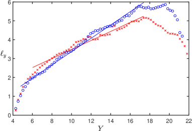
Figure 10: Horizontal integral turbulent scale $\ell_{y}$ versus $Y$ averaged over $Z$ for isothermal turbulence (red); fitting: $\ell_{y}=0.24Y+0.96$ (solid) from $Y=$ 6 cm to 17.3 cm and temperature stratified turbulence (blue); $\ell_{y}=0.36Y-0.33$ (solid) from $Y=$ 4.7 cm to 17.3 cm. The integral scale and coordinates are measured in cm.

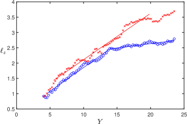
Figure 11: Vertical integral turbulent scale $\ell_{z}$ versus $Y$ averaged over $Z$ for isothermal turbulence (red); fitting: $\ell_{z}=0.15Y+0.6$ (solid) from $Y=$ 5.5 cm to 19.8 cm and temperature stratified turbulence (blue); fitting: $\ell_{z}=0.155Y+0.3$ (solid) from $Y=$ 4.5 cm to 13.5 cm and $\ell_{z}=0.027Y+2.08$ from $Y=$ 13.5 cm to 23.7 cm. The integral scale and coordinates are measured in cm.

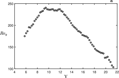
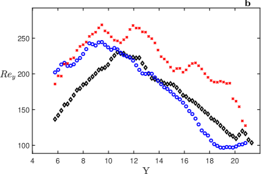
Figure 12: Reynolds number Re${}_{y}=u^{\rm(rms)}_{y}\,\ell_{y}/\nu$ in the horizontal direction versus $Y$ (a) averaged over $Z$ (upper panel) or (b) averaged over different vertical regions (lower panel): $Z=4.3-9.6$ cm (red, slanting crosses); $Z=9.6-15$ cm (blue, circles); $Z=15-20$ cm (black, diamond) for temperature stratified turbulence.

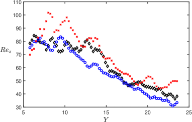
Figure 13: Reynolds number Re${}_{z}=u^{\rm(rms)}_{z}\,\ell_{z}/\nu$ in the vertical direction versus $Y$ averaged over different vertical regions: $Z=4.3-9.6$ cm (red, slanting crosses); $Z=9.6-15$ cm (blue, circles) and $Z=15-20$ cm (black, diamond) for temperature stratified turbulence.

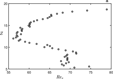
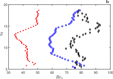
Figure 14: Reynolds number Re${}_{z}=u^{\rm(rms)}_{z}\,\ell_{z}/\nu$ in the vertical direction versus $Z$ (a) averaged over $Y$ (upper panel) or (b) averaged over different horizontal regions (lower panel): $Y=4-10$ cm (black, diamond); $Y=10-17$ cm (blue, circles) and $Y=17-23$ cm (red, slanting crosses) for temperature stratified turbulence.

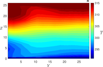
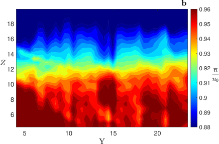
Figure 15: Distributions of (a) the mean temperature $\overline{T}(Y,Z)$ (upper panel) and (b) normalized mean particle number density $\overline{n}(Y,Z)/\overline{n}_{0}$ (lower panel) for temperature stratified turbulence. Temperature is measured in K and coordinates are measured in cm.

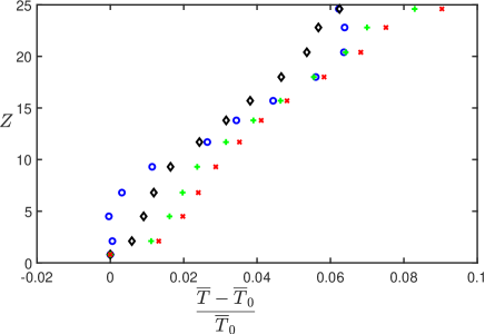
Figure 16: Vertical profiles of the relative normalized mean temperature $(\overline{T}-\overline{T}_{0})/\overline{T}_{0}$ averaged over different horizontal regions: $Y=0.5-6.5$ cm (blue, circles); $Y=8.5-14.5$ cm (black, diamond); $Y=16.5-22.5$ cm (green, crosses) and $Y=24.5-28.5$ cm (red, slanting crosses).

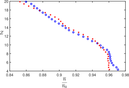
Figure 17: Vertical profiles of the normalized mean particle number density $\overline{n}/\overline{n}_{0}$ averaged over different horizontal regions: $Y=4-15$ cm (blue, circles) and $Y=15-24$ cm (slanting crosses) for temperature stratified turbulence.

In Figs. 2 and 3 we show mean velocity patterns $\overline{U}$ in the core flow for isothermal turblulence and temperature stratified turbulence. All measurements of the velocity field in the horizontal direction $Y$ are performed starting 20 cm away from the left wall of the chamber where the grid is located. The amplitude of the grid oscillations is 6 cm, and velocity is measured beginning of the distance 4 cm away from the oscillating grid. Figures 2and 3 demonstrates that the nonuniform mean temperature field affects the mean velocity patterns.

In Figs. 4 and 5 we plot turbulent velocities $u^{\rm(rms)}_{y}$ and $u^{\rm(rms)}_{z}$ versus $Y$ averaged over different vertical regions (see for details, captions of Figs. 4 and 5) for isothermal and temperature stratified turbulence. In Fig. 6 and 7 we also show turbulent velocities $u^{\rm(rms)}_{y}$ and $u^{\rm(rms)}_{z}$ versus $Y$ averaged over $Z$ (without the separation to different vertical regions) for isothermal and temperature stratified turbulence. The differences in the turbulent velocities for isothermal and temperature stratified turbulence are not essential. This is also seen in Figs. 8 and 9 where we show the counter lines for the horizontal and vertical components of the turbulent velocity in the $YZ$ plane for isothermal and temperature stratified turbulence.

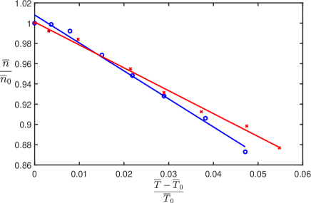
Figure 18: The normalized mean particle number density $\overline{n}/\overline{n}_{0}$ versus the relative normalized mean temperature $(\overline{T}-\overline{T}_{0})/\overline{T}_{0}$ averaged over different horizontal regions: $Y=4-15$ cm (blue, circles) and $Y=15-24$ cm (red, slanting crosses) for temperature stratified turbulence.

In Figs. 10 and 11 we plot the integral turbulent scales $\ell_{y}$ and $\ell_{z}$ in horizontal and vertical directions versus $Y$ averaged over $Z$ for isothermal and temperature stratified turbulence. In both cases, in isothermal and temperature stratified turbulence, the vertical component of the turbulent velocity $u^{\rm(rms)}_{z}$ decreases as $Y^{-1}$, while the integral turbulent scales $\ell_{y}$ and $\ell_{z}$ increase linearly with the distance from the grid $Y$ in agreement with previous studies for isothermal turbulence in water experiments [42, 43, 44, 45, 46, 47, 48].

Using the obtained turbulent velocities $u^{\rm(rms)}_{i}$ and the integral turbulence scales $\ell_{i}$, we determine the Reynolds numbers in the horizontal $\left({\rm Re}_{y}=u^{\rm(rms)}_{y}\,\ell_{y}/\nu\right)$ and the vertical $\left({\rm Re}_{z}=u^{\rm(rms)}_{z}\,\ell_{z}/\nu\right)$ directions as functions of horizontal coordinate $Y$ (see Figs. 12 and 13). In a similar way, we determine the vertical profiles of Re_z plotted in Fig. 14. The Reynolds numbers ${\rm Re}_{y}$ in the horizontal direction are essentially larger than the Reynolds numbers ${\rm Re}_{z}$ in the vertical direction, because the turbulent velocities and the integral turbulence scales are larger in the horizontal direction.

The Stokes number for particles used in our experiments varies in the range from $5\times 10^{-6}$ far from the grid to $2\times 10^{-4}$ near the grid. In particular, the Stokes time for particles having the diameter 0.7 $\mu$m is $1.5\times 10^{-6}$ s, and the Kolmogorov time varies from $7\times 10^{-3}$ s in turbulence near the grid to $0.3$ s in turbulence far from the grid.

The initial distribution of particles injected into the chamber is nearly homogeneous. Turbulent thermal diffusion results in formation of strongly inhomogeneous particle distributions. Sedimentation of particles is very weak in our experiments, since the terminal fall velocity for particles having the mean diameter $0.7\mu$m is about $10^{-2}$ cm/s. Characteristic turbulent velocity (that is about $12$ cm/s near the grid and is about $2$ cm/s far from the grid) and the effective pumping velocity caused by turbulent thermal diffusion (that is about $1$ cm/s near the grid and is about $0.1$ cm/s far from the grid) are much larger than the terminal fall velocity.

Measurements of temperature and particle number density allow us to determine spatial distribution of the mean temperature $\overline{T}$ and the normalized mean particle number density $\overline{n}/\overline{n}_{0}$ (see Fig. 15). Inspection of Fig. 15 shows that particles are accumulated in the vicinity of the minimum of the mean temperature (i.e., in the vicinity of the bottom wall of the chamber) due to phenomenon of turbulent thermal diffusion.

In Fig. 16 we show vertical profiles of the relative normalized mean temperature $(\overline{T}-\overline{T}_{0})/\overline{T}_{0}$ averaged over different horizontal regions (see the caption of Fig. 16), where $\overline{T}_{0}$ is the reference mean temperature. In Fig. 17 we plot the normalized mean particle number density $\overline{n}/\overline{n}_{0}$ averaged over different horizontal regions (see the caption of Fig. 17), where $\overline{n}_{0}=\overline{n}(\overline{T}=\overline{T}_{0})$. The normalized mean temperature increases linearly with the height $Z$ in the flow core (see Fig. 16), while the normalized mean particle number density decreases linearly with the height $Z$ (see Fig. 17).

The vertical profiles of the mean temperature and the mean particle number density allow us to determine the normalized mean particle number density $\overline{n}/\overline{n}_{0}$ versus the relative normalized mean temperature $(\overline{T}-\overline{T}_{0})/\overline{T}_{0}$ (see Fig. 18). The slope of this dependence allows us to find the effective turbulent thermal diffusion coefficient $\alpha$ for particles in inhomogeneous and anisotropic stably stratified turbulence. Indeed, the steady-state solution (12) of the equation for the mean particle number density yields $\delta\overline{n}/\overline{n}_{0}=-\alpha\,\delta\overline{T}/\overline{T}_{0}$, where we take into account that $D_{\rm T}\gg D$. This equation can be rewritten as $\overline{n}/\overline{n}_{0}=1-\alpha\,(\overline{T}-\overline{T}_{0})/\overline{T}_{0}$. Using this equation, we find from Fig. 13, that $\alpha=2.765$ for particles accumulated in the regions $Y=4-15$ cm, and $\alpha=2.26$ for particles accumulated in the regions $Y=16-24$ cm. For the second region that is far from the grid, the level of turbulence is lower than that for the first region. This explains the difference in the effective turbulent thermal diffusion coefficient $\alpha$ determined for these regions. This experimental study has clearly detected phenomenon of turbulent thermal diffusion in an inhomogeneous turbulence.

V Conclusions

Turbulent thermal diffusion of particles in inhomogeneous stably stratified turbulence produced by one oscillating grid in the air flow has been studied. Measurements of the velocity fields using a Particle Image Velocimetry (PIV) allow us to determine the mean and the r.m.s. velocities, two-point correlation functions of the velocity field and an integral scale of turbulence. Spatial distributions of the temperature field have been determined using a temperature probe equipped with 12 E – thermocouples. We also determine the spatial distributions of particles by means of the PIV system using the effect of the Mie light scattering by particles in the flow. The experiments have shown that particles are accumulated at the vicinity of the minimum of the mean temperature due to the phenomenon of turbulent thermal diffusion. The obtained spatial distributions of particles and temperature fields allow us to determine the effective turbulent thermal diffusion coefficient of particles in inhomogeneous temperature stratified turbulence. This coefficient varies from $2.765$ for particles accumulated in the vicinity of the cold wall of the chamber in the regions more close to the grid to $2.26$ for particles accumulated in the regions far from the grid where turbulence is less intensive. These values are in agreement with theoretical predictions [33] for the micron-size particles.

DATA AVAILABILITY

The data that support the findings of this study are available from the corresponding author upon reasonable request.

References

- [1] G. T. Csanady, Turbulent Diffusion in the Environment (Reidel, Dordrecht, 1980).
- [2] Ya. B. Zeldovich, A. A. Ruzmaikin, and D. D. Sokoloff, The Almighty Chance (Word Scientific Publ., Singapore, 1990).
- [3] A. K. Blackadar, Turbulence and Diffusion in the Atmosphere (Springer, Berlin, 1997).
- [4] J. H. Seinfeld and S. N. Pandis, Atmospheric Chemistry and Physics. From Air Pollution to Climate Change., 2nd ed. (John Wiley & Sons, NY, 2006).
- [5] L. I. Zaichik, V. M. Alipchenkov, and E. G. Sinaiski, Particles in turbulent flows (John Wiley & Sons, NY, 2008).
- [6] C. T. Crowe, J. D. Schwarzkopf, M. Sommerfeld and Y. Tsuji, Multiphase flows with droplets and particles, second edition (CRC Press LLC, NY, 2011).
- [7] I. Rogachevskii, Introduction to Turbulent Transport of Particles, Temperature and Magnetic Fields (Cambridge University Press, Cambridge, 2021).
- [8] Z. Warhaft, Passive scalars in turbulent flows, Annu. Rev. Fluid Mech. 32, 203 (2000).
- [9] R. A. Shaw, Particle-turbulence interactions in atmospheric clouds, Annu. Rev. Fluid Mech. 35, 183 (2003).
- [10] A. Khain, M. Pinsky, T. Elperin, N. Kleeorin, I. Rogachevskii and A. Kostinski, Critical comments to results of investigations of drop collisions in turbulent clouds, Atmosph. Res. 86, 1 (2007).
- [11] A. Guha, Transport and deposition of particles in turbulent and laminar flow, Annu. Rev. Fluid Mech. 40, 311 (2008).
- [12] Z. Warhaft, Laboratory studies of droplets in turbulence: towards understanding the formation of clouds, Fluid Dyn. Res. 41, 011201 (2009).
- [13] J. Bec, L. Biferale, M. Cencini, A. Lanotte, S. Musacchio and F. Toschi, Heavy particle concentration in turbulence at dissipative and inertial scales, Phys. Rev. Lett. 98, 084502 (2007).
- [14] F. Toschi and E. Bodenschatz, Lagrangian properties of particles in turbulence, Annu. Rev. Fluid Mech. 41, 375 (2009).
- [15] S. Balachandar and J. K. Eaton, Turbulent dispersed multiphase flow, Annu. Rev. Fluid Mech. 42, 111 (2010).
- [16] T. Elperin, N. Kleeorin, I. Rogachevskii, Self-excitation of fluctuations of inertial particles concentration in turbulent fluid flow, Phys. Rev. Lett. 77, 5373 (1996).
- [17] T. Elperin, N. Kleeorin, V. L’vov, I. Rogachevskii, D. Sokoloff, Clustering instability of the spatial distribution of inertial particles in turbulent flows, Phys. Rev. E 66, 036302 (2002).
- [18] M. van Aartrijk and H. J. H. Clercx, Preferential concentration of heavy particles in stably stratified turbulence, Phys. Rev. Lett. 100, 254501 (2008).
- [19] A. Eidelman, T. Elperin, N. Kleeorin, B. Melnik and I. Rogachevskii, Tangling clustering of inertial particles in stably stratified turbulence, Phys. Rev. E 81, 056313 (2010).
- [20] T. Elperin, N. Kleeorin, M. A. Liberman and I. Rogachevskii, Tangling clustering instability for small particles in temperature stratified turbulence, Phys. Fluids 25, 085104 (2013).
- [21] M. Caporaloni, F. Tampieri, F. Trombetti and O. Vittori, Transfer of particles in nonisotropic air turbulence, J. Atmosph. Sci. 32, 565 (1975).
- [22] M. Reeks, The transport of discrete particle in inhomogeneous turbulence, J. Aerosol Sci. 14, 729 (1983).
- [23] A. Guha, A unified Eulerian theory of turbulent deposition to smooth and rough surfaces, J. Aerosol Sci. 28, 1517 (1997).
- [24] T. Elperin, N. Kleeorin and I. Rogachevskii, Formation of inhomogeneities in two-phase low-Mach-number compressible turbulent fluid flows, Int. J. Multiphase Flow 24, 1163 (1998).
- [25] Dh. Mitra, N. E. L. Haugen and I. Rogachevskii, Turbophoresis in forced inhomogeneous turbulence, Europ. Phys. J. Plus 133, 35 (2018).
- [26] T. Elperin, N. Kleeorin and I. Rogachevskii, Turbulent thermal diffusion of small inertial particles, Phys. Rev. Lett. 76, 224 (1996).
- [27] T. Elperin, N. Kleeorin and I. Rogachevskii, Turbulent barodiffusion, turbulent thermal diffusion and large-scale instability in gases, Phys. Rev. E 55, 2713 (1997).
- [28] T. Elperin, N. Kleeorin and I. Rogachevskii, Mechanisms of formation of aerosol and gaseous inhomogeneities in the turbulent atmosphere, Atmosph. Res. 53, 117 (2000).
- [29] T. Elperin, N. Kleeorin, I. Rogachevskii and D. Sokoloff, Passive scalar transport in a random flow with a finite renewal time: Mean-field equations, Phys. Rev. E 61, 2617 (2000).
- [30] T. Elperin, N. Kleeorin, I. Rogachevskii and D. Sokoloff, Mean-field theory for a passive scalar advected by a turbulent velocity field with a random renewal time, Phys. Rev. E 64, 026304 (2001).
- [31] R. V. R. Pandya and F. Mashayek, Turbulent thermal diffusion and barodiffusion of passive scalar and dispersed phase of particles in turbulent flows, Phys. Rev. Lett. 88, 044501 (2002).
- [32] M. W. Reeks, On model equations for particle dispersion in inhomogeneous turbulence, Int. J. Multiph. Flow 31, 93 (2005).
- [33] G. Amir, N. Bar, A. Eidelman, T. Elperin, N. Kleeorin and I. Rogachevskii, Turbulent thermal diffusion in strongly stratified turbulence: Theory and experiments, Phys. Rev. Fluids 2, 064605 (2017).
- [34] J. Buchholz, A. Eidelman, T. Elperin, G. Grünefeld, N. Kleeorin, A. Krein, I. Rogachevskii, Experimental study of turbulent thermal diffusion in oscillating grids turbulence, Experim. Fluids 36, 879 (2004).
- [35] A. Eidelman, T. Elperin, N. Kleeorin, A. Krein, I. Rogachevskii, J. Buchholz, and G. Grünefeld, Turbulent thermal diffusion of aerosols in geophysics and in laboratory experiments, Nonl. Proc. Geophys. 11, 343 (2004).
- [36] A. Eidelman, T. Elperin, N. Kleeorin, A. Markovich, I. Rogachevskii, Experimental detection of turbulent thermal diffusion of aerosols in non-isothermal flows, Nonl. Proc. Geophys. 13, 109 (2006).
- [37] A. Eidelman, T. Elperin, N. Kleeorin, I. Rogachevskii and I. Sapir-Katiraie, Turbulent thermal diffusion in a multi-fan turbulence generator with the imposed mean temperature gradient, Experim. Fluids 40, 744 (2006).
- [38] N. E. L. Haugen, N. Kleeorin, I. Rogachevskii and A. Brandenburg, Detection of turbulent thermal diffusion of particles in numerical simulations, Phys. Fluids 24, 075106 (2012).
- [39] I. Rogachevskii, N. Kleeorin and A. Brandenburg, Compressibility in turbulent magnetohydrodynamics and passive scalar transport: mean-field theory, J. Plasma Phys. 84, 735840502 (2018).
- [40] M. Sofiev, V. Sofieva, T. Elperin, N. Kleeorin, I. Rogachevskii and S. S. Zilitinkevich, Turbulent diffusion and turbulent thermal diffusion of aerosols in stratified atmospheric flows, J. Geophys. Res. 114, D18209 (2009).
- [41] A. Hubbard, Turbulent thermal diffusion: a way to concentrate dust in protoplanetary discs, Monthly Notes Roy. Astron. Soc. 456, 3079-3089 (2016).
- [42] J. S. Turner, The influence of molecular diffusivity on turbulent entrainment across a density interface, J. Fluid Mech. 33, 639-656 (1968).
- [43] Turner, S. T., Buoyancy Effects in Fluids (Cambridge Univ. Press, Cambridge, 1973).
- [44] S. M. Thompson and J. S. Turner, Mixing across an interface due to turbulence generated by an oscillating grid, J. Fluid Mech. 67, 349-368 (1975).
- [45] E. J. Hopfinger and J.-A. Toly, Spatially decaying turbulence and its relation to mixing across density interfaces, J. Fluid Mech. 78, 155-175 (1976).
- [46] E. Kit, E. J. Strang and H. J. S. Fernando, Measurement of turbulence near shear-free density interfaces, J. Fluid Mech. 334, 293-314 (1997).
- [47] M. A. Snchez and J. M. Redondo, Observations from grid stirred turbulence, Appl. Sci. Res. 59, 243-254 (1998).
- [48] P. Medina, M. A. Snchez and J. M. Redondo, Grid stirred turbulence: applications to the initiation of sediment motion and lift-off studies, Phys. Chem. Earth B 26, 299-304 (2001).
- [49] S. Chandrasekhar, Stochastic problems in physics and astronomy, Rev. Modern Phys. 15, 1 (1943).
- [50] A. I. Akhiezer and S. V. Peletminsky, Methods of Statistical Physics (Pergamon, Oxford, 1981).
- [51] M. R. Maxey, The gravitational settling of aerosol particles in homogeneous turbulence and random flow field, J. Fluid Mech. 174, 441 (1987).
- [52] R. J. Adrian, Particle-imaging tecniques for experimental fluid mechanics, Annu. Rev. Fluid Mech. 23, 261 (1991).
- [53] M. Raffel, C. Willert, S. Werely and J. Kompenhans, Particle Image Velocimetry (Springer, Berlin-Heidelberg, 2007).
- [54] J. Westerweel, Theoretical analysis of the measurement precision in particle image velocimetry, Experim. Fluids 29, S3 (2000).
- [55] P. Guibert, M. Durget and M. Murat, Concentration fields in a confined two-gas mixture and engine in cylinder flow: laser tomography measurements by Mie scattering, Experim. Fluids 31, 630-642 (2001).
- [56] C. F. Bohren and D. R. Huffman, Absorbtion and Scattering of Light by Small Particles (John Wiley and Sons, New York, 1983).
- [57] M. Bukai, A. Eidelman, T. Elperin, N. Kleeorin, I. Rogachevskii and I. Sapir-Katiraie, Effect of large-scale coherent structures on turbulent convection, Phys. Rev. E 79, 066302 (2009).
- [58] M. Bukai, A. Eidelman, T. Elperin, N. Kleeorin, I. Rogachevskii and I. Sapir-Katiraie, Transition phenomena in unstably stratified turbulent flows, Phys. Rev. E 83, 036302 (2011).
- [59] A. Eidelman, T. Elperin, I. Gluzman, N. Kleeorin and I. Rogachevskii, Experimental study of temperature fluctuations in forced stably stratified turbulent flows, Phys. Fluids 25, 015111 (2013).