Explorations of pseudo-Dirac dark matter having keV splittings and interacting via transition electric and magnetic dipole moments

Abstract

We study a minimal model of pseudo-Dirac dark matter, interacting through transition electric and magnetic dipole moments. Motivated by the fact that xenon experiments can detect electrons down to $\sim$ keV recoil energies, we consider $\mathcal{O}$(keV) splittings between the mass eigenstates. We study the production of this dark matter candidate via the freeze-in mechanism. We discuss the direct detection signatures of the model arising from the down-scattering of the heavier state, that are produced in Solar upscattering, finding observable signatures at the current and near-future xenon based direct detection experiments. We also study complementary constraints on the model from fixed target experiments, lepton colliders, supernovae cooling and cosmology. We show that the latest XENONnT results rule out parts of the parameter space for this well motivated and minimal dark matter candidate. Next generation xenon experiments can either discover or further constrain how strongly inelastic dark matter can interact via the dipole moment operators.

I Introduction

The identity of dark matter (DM) is one of the most important questions in science. Multiple broad approaches are pursued in order to address this important question Green:2021jrr ; Cooley:2021rws ; Slatyer:2021qgc . One of the frontiers of DM physics today can be understood to lie along the reach of current detection methodologies looking to identify the particle nature of DM and/ or its interactions with Standard Model (SM) particles, pushed farther along by the projections of near future detectors. From this perspective, hints of anomalies in data as well as new detectors that achieve improved efficiency and background control make for exciting progress and spur new investigations into the physics of DM. One such result came from the XENON1T experiment XENON:2020rca that reported a $3\sigma$ excess in the electron recoil spectrum between $2-3$ keV and attracted wide attention from the perspective of DM interpretation An:2020bxd ; Baryakhtar:2020rwy ; Keung:2020uew ; Takahashi:2020bpq ; Choudhury:2020xui ; Harigaya:2020ckz ; Cao:2020bwd ; Fornal:2020npv ; Ko:2020gdg ; Su:2020zny ; Alonso-Alvarez:2020cdv ; Lee:2020wmh ; Bramante:2020zos ; Paz:2020pbc ; Nakayama:2020ikz ; Bell:2020bes ; Chen:2020gcl ; Chao:2020yro ; Smirnov:2020zwf ; Kannike:2020agf ; Boehm:2020ltd ; Du:2020ybt ; Choi:2020udy ; Buch:2020mrg ; Dey:2020sai ; Jho:2020sku ; Bloch:2020uzh ; Lindner:2020kko ; Budnik:2020nwz ; Zu:2020idx ; Gao:2020wer ; DeRocco:2020xdt ; Dent:2020jhf ; McKeen:2020vpf ; DelleRose:2020pbh ; Alhazmi:2020fju ; An:2020tcg ; Croon:2020ehi ; Chigusa:2020bgq ; Okada:2020evk ; Davighi:2020vap ; Choi:2020kch ; Baek:2020owl ; Davoudiasl:2020ypv ; Chiang:2020hgb ; He:2020wjs ; Long:2020uyf ; Croon:2020oga ; Arcadi:2020zni ; Ema:2020fit ; Khan:2020pso ; Farzan:2020llg ; Zu:2020bsx ; Lasenby:2020goo ; Chakraborty:2020vec ; Guo:2020oum ; Aboubrahim:2020iwb ; Buttazzo:2020vfs ; Choi:2020ysq ; He:2020sat ; Jia:2020omh ; Xu:2020qsy ; Dutta:2021wbn ; Bell:2021zkr ; Dutta:2021nsy ; Baek:2021yos ; PandaX-II:2020udv ; Dror:2019dib ; Dror:2019onn ; Dror:2020czw ; Borah:2020jzi ; Borah:2021yek ; Emken:2021vmf ; Borah:2021jzu or for background considerations Robinson:2020gfu ; Bhattacherjee:2020qmv ; Szydagis:2020isq . It also reported a background rate of $76\pm 2$ events$/(\textrm{tonne}\times\textrm{year}\times\textrm{keV})$ for electron recoil energies between $1-30$ keV. Subsequently, this background was reduced to $15.8\pm 1.3$  events$/(\textrm{tonne}\times\textrm{year}\times\textrm{keV})$ by the XENONnT experiment XENONCollaboration:2022kmb , while observing no excess, with an exposure of 1.16 tonne$\times$years.

The scattering of typical WIMP-like DM, with velocity distributions following the Standard Halo Model, against electrons lead to recoil energies of $\mu_{e,DM}v_{DM}^{2}\sim\mathcal{O}$(eV), where $\mu_{e,DM}$ is the electron-DM reduced mass and $v_{DM}$ is the incoming DM velocity. The $\mathcal{O}$(keV) recoil energies that XENON1T probes currently can broadly arise from various DM models like boosted DM Fornal:2020npv ; Su:2020zny ; Cao:2020bwd ; Ko:2020gdg ; Chen:2020gcl that acquire higher velocities than the typical DM halo velocities, absorption of $\mathcal{O}$(keV) particles Takahashi:2020bpq , or through down-scattering of inelastic DM with two nearly degenerate DM states with mass splittings of $\mathcal{O}$(keV) Baryakhtar:2020rwy ; Keung:2020uew ; Harigaya:2020ckz ; Lee:2020wmh ; An:2020tcg ; Chao:2020yro . The coincidence of similarity in the recoil energies probed by XENONnT and the temperature at the Sun’s core ($\sim$ 1.1 keV) motivates the study of inelastic DM which is upscattered in the Sun. Specifically, if the heavier particle is not cosmologically stable, and the lighter particle constitutes the DM, they can be excited to the heavier particle by upscattering against Solar electrons. It can subsequently down-scatter via electron scatterings at XENONnT, depositing an energy approximately equal to the mass splitting.

With this in mind, we study the most minimal model of pseudo-Dirac DM with two Majorana fermions. The lowest dimension interactions with SM allowed, in the absence of any additional dark sector particles, are the transition electric and magnetic dipole moments. Dipolar DM Masso:2009mu ; Blanchet:2009zu with scattering processes mediated by the photon, gives enhanced scattering rates in the small velocity limit applicable in terrestrial direct detection (DD) experiments Hambye:2018dpi . We therefore study:

• The freeze-in (FI) production McDonald:2001vt ; Hall:2009bx of pseudo-Dirac DM with mass splittings of $\mathcal{O}$(keV).

• The DD of this DM via up-scattering in the Sun followed by down-scattering in electron recoil events at the XENONnT experiment (as well as projections for future runs of XENONnT and DARWIN). We study the DD rates for generic parts of the parameter space without the relic density constraint from FI production.

• Complementary bounds on generic parts of the parameter space. These include constraints from fixed target experiments, lepton colliders, SN1987A and $N_{\rm eff}$ constraints.

Inelastic DM with interaction via transition dipolar moments have previously been studied with focus on different parameter spaces Weiner:2012cb ; Patra:2011aa ; Masso:2009mu . Refs. CarrilloGonzalez:2021lxm ; Filimonova:2022pkj ; Herrera:2023fpq have also studied pseudo-Dirac type DM in a dark photon model. Dipolar DM motivated by lepton sector minimal flavor violation was recently studied in DAmbrosio:2021wpd .

In section II, we discuss our model and the production of the DM via FI mechanism. In section III, we discuss the signatures at DD experiments from electron and nuclear scatterings. In section IV, we discuss complementary bounds on the model from various existing experiments and observations. Finally, we present the results in section V and conclude in section VI.

II Model Framework and Freeze-in Production

We consider a dark sector consisting of two Majorana fermions $\chi_{1}$ and $\chi_{2}$ that form a pseudo-Dirac state with mass splitting $\delta\equiv m_{\chi_{2}}-m_{\chi_{1}}\sim\mathcal{O}(\textrm{keV})$. The lowest dimension interaction operators allowed in the absence of any additional new particles are through the DM dipole moments where the interaction is mediated by photons. Since the only dipolar type interactions that are allowed for Majorana fermions are of transition type, we get the following Lagrangian for DM interaction Masso:2009mu

$$\mathcal{L}_{DM}\supset\underbrace{\frac{\mu_{\chi}}{2}\bar{\chi}_{1}\sigma_{\mu\nu}\chi_{2}\,F^{\mu\nu}}_{MDM}+\underbrace{i\frac{d_{\chi}}{2}\bar{\chi}_{1}\sigma_{\mu\nu}\gamma_{5}\chi_{2}\,F^{\mu\nu}}_{EDM},$$ (1)

where $\mu_{\chi}$ and $d_{\chi}$ are the transition magnetic dipole moment (MDM) and electric dipole moment (EDM), respectively.

We consider the production of DM by the FI mechanism which is operative when the DM coupling to SM is small enough for the DM to have never entered thermal equilibrium with the SM bath. With an assumption of negligible DM number density at the earliest epoch, it is produced via annihilation and decay of SM particles; some relevant Feynman diagrams for dipolar DM are shown in fig. 1. As the temperature of SM bath falls, the DM production ceases as follows. For $m_{DM}>m_{SM}$, as the bath temperature falls below the DM mass, the DM production becomes kinematically suppressed. While for $m_{SM}>m_{DM}$, as the bath temperature falls below the SM particle mass, it freezes out and its annihilation rate is suppressed. Thus the DM number density per comoving volume becomes a constant, and the DM is said to have frozen into the current relic abundance.

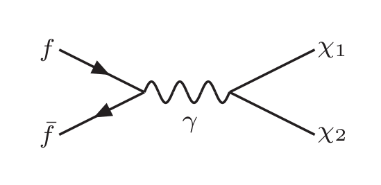
(a)

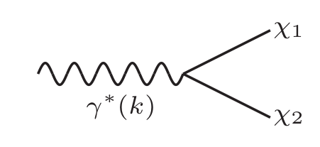
(b)

Figure 1: Two example processes for FI production of dipolar DM: (a) $2\rightarrow 2$ annihilation production from SM fermions (we do not show here the diagram for production from $W^{+}W^{-}$) and (b) production from plasmon decay.

We solve the Boltzmann equation to calculate the DM relic density. For convenience, we define the number per co-moving volume as Yield, $Y\equiv n/s$, with $n$ representing the number density and $s$ being the entropy density. The Boltzmann equation then gives McDonald:2001vt ; Hall:2009bx ; Dutra:2019gqz

$$\frac{dY}{dT}=-\left(\frac{45}{\pi}\right)^{3/2}\frac{M_{Pl}}{4\pi^{2}g_{\star}^{s}\sqrt{g_{\star}}}\left(1+\frac{1}{3}\frac{d\,ln\,g_{\star}}{d\,ln\,T}\right)\frac{R(T)}{T^{6}},$$ (2)

where T is the temperature of the SM bath, $M_{Pl}$ is the Planck mass, $g^{s}_{*}$ and $g_{*}$ are the temperature dependent relativistic degrees of freedom contributing to entropy and energy densities, respectively. $R(T)$ is the rate for DM production and is a sum of rates of production from $2\rightarrow 2$ annihilation, $R_{2\rightarrow 2}$, and from the decay of plasmon, $R_{\gamma^{*}}$,

$$R(T)=R_{2\rightarrow 2}(T)+R_{\gamma^{*}}(T).$$ (3)

We discuss these two modes of production in the following subsections.

The total DM relic density is

$$\Omega\,h^{2}=\frac{Y(T_{0})\,s(T_{0})m_{\chi_{1}}h^{2}}{\rho_{crit}}=Ym_{\chi_{1}}h^{2}\frac{2.89\times 10^{9}\,\text{m}^{-3}}{10.5\,h^{2}\,\text{GeVm}^{-3}}=Ym_{\chi_{1}}\frac{2.89\times 10^{9}\,\text{m}^{-3}}{10.5\,\text{GeVm}^{-3}},$$ (4)

where we have assumed only the lighter particle $\chi_{1}$ with mass $m_{\chi_{1}}$ to be stable on cosmological timescales. Here, $\rho_{crit}$ is the critical density and $T_{0}$ is the temperature of current epoch, with the values for the physical constants taken from ref. Belanger:2018ccd .

II.1 Annihilation production

The rate of production of particles $\chi_{1},\chi_{2}$ from the annihilation of SM fermions, as shown in fig. 1 (a), is Hall:2009bx ; Bernal:2017kxu ; Dutra:2019gqz

$$R_{2\rightarrow 2}(T) = \sum_{f}N_{c}^{f}\frac{T}{(2\pi)^{6}2^{4}}\int_{s_{min}}^{\infty}ds\sqrt{s-4m_{f}^{2}}\frac{|\vec{p}_{3}^{\,\,0}|}{\sqrt{m_{\chi_{1}}^{2}+|\vec{p}_{3}^{\,\,0}|^{2}}+\sqrt{m_{\chi_{2}}^{2}+|\vec{p}_{3}^{\,\,0}|^{2}}}$$ (5)

$$\times\,K_{1}\left(\frac{\sqrt{s}}{T}\right)\int d\Omega_{3}^{\star}\,|\mathcal{M}|^{2},$$

where $N_{c}^{f}$ are the color degrees of freedom of SM fermion $f$ with mass $m_{f}$. The total rate is a sum over the SM fermions $f$. $K_{1}$ is the modified Bessel function of the second kind, $s_{min}=\textrm{Max}\left[(m_{\chi_{1}}+m_{\chi_{2}})^{2},4m_{f}^{2}\right]$, and the 3-momentum of $\chi_{1}$ in the center-of-mass (CM) frame is

$$|\vec{p}_{3}^{\,\,0}|=\sqrt{\left(\frac{\sqrt{s}}{2}+\frac{m_{\chi_{1}}^{2}-m_{\chi_{2}}^{2}}{2\sqrt{s}}\right)^{2}-m_{\chi_{1}}^{2}}.$$

The squared-amplitude $|\mathcal{M}|^{2}$ is summed over initial and final spins Masso:2009mu

$$\int d\Omega_{3}^{\star}\sum\big{|}\mathcal{M}\big{|}_{f}^{2}\simeq\begin{cases}32\pi d_{\chi}^{2}e^{2}q_{f}^{2}\frac{(s-4m_{\chi_{1}}^{2})(s+2m_{f}^{2})}{3s}-128\pi\,\delta d_{\chi}^{2}e^{2}q_{f}^{2}\frac{m_{\chi_{1}}(s+2m_{f}^{2})}{3s}+\mathcal{O}(\delta^{2}),&\text{ for EDM,}\\ 32\pi\mu_{\chi}^{2}e^{2}q_{f}^{2}\frac{(s+8m_{\chi_{1}}^{2})(s+2m_{f}^{2})}{3s}+64\pi\,\delta\mu_{\chi}^{2}e^{2}q_{f}^{2}\frac{m_{\chi_{1}}(s+2m_{f}^{2})}{3s}+\mathcal{O}(\delta^{2}),&\text{ for MDM,}\end{cases}$$ (6)

where we give the expressions upto leading order in $\delta\equiv m_{\chi_{2}}-m_{\chi_{1}}$. In the limit of vanishing SM fermion and DM masses, we find that the production rate scales with temperature as $R(T)\propto T^{6}$. From eq. (2), we see that this leads to UV (UltraViolet) FI with maximum yield produced at the largest temperature of the SM bath, equal to the reheating temperature for models with instantaneous reheating Chen:2017kvz ; Elahi:2014fsa ; Chowdhury:2018tzw ; Giudice:2000ex .

Of phenomenological interest is the parameter space with large coupling which can lead to large scattering rate at DD experiments. We note that for $m_{DM}\geq T_{RH}$, there is kinematic suppression in DM production, requiring large couplings to reproduce the observed relic density. For the light DM we consider in this work, $m_{DM}\leq 1\,{\rm GeV}$, we choose low reheating temperatures ($T_{RH}$ = 5 MeV and 10 MeV) from allowed values. We verify our calculations using the expressions given above, with those obtained from micrOMEGAs 5.0 Belanger:2018ccd , for fermionic channels of production.

We discuss the results in section V.

II.2 Plasmon decay

The SM bath consists of charged particles that couple to the photon. An electromagnetic wave propagating through this bath behaves qualitatively differently from that in vacuum. Coherent vibrations of the electromagnetic field and the density of charged particles results in a spin-1 particle with 1 longitudinal and 2 transverse polarizations, propagating at a speed less than the speed of light in vacuum. Its dispersion relation depends on the properties of the SM plasma and is therefore known as the ‘plasmon’. We follow the discussion in refs. Braaten:1993jw ; Raffelt:1996wa for the plasmon properties and decay rates.

The significance of plasmon decay leading to production of DM in FI scenarios was noted in ref. Dvorkin:2019zdi (see also Chu:2019rok ; Chang:2019xva ; Hambye:2019dwd ). The massive plasmon can decay to DM in cases where the DM couples to the photon. This is true in the dipolar interaction case we study here. For DM produced via FI mechanism, the final abundance is accumulated over time and summed over the various production channels of SM particles annihilating and decaying to DM. Therefore, the production from plasmon decay can play a significant role in FI produced DM (as opposed to freeze-out production).

To calculate the DM abundance resulting from plasmon decay, we must begin with the modified dispersion relations which depend on the temperature $T$ and the net density of the charged particles in the SM plasma. Since ref. Braaten:1993jw was addressing the energy loss from the plasma in a supernova with typical energies of $\mathcal{O}(10)$ MeV, only electrons and positrons were considered as charged particles of relevance that modify the dispersion relations. But for the case of a UV FI with large enough $T_{RH}$, all charged particles with masses much smaller than the reheating temperature would add to the plasmon effect (see appendix A for further details). The rate of DM production from plasmon decay is

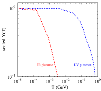
Figure 2: Production of DM from plasmon decay, for IR and UV ($T_{RH}=1$ GeV) FI models. We consider $m_{DM}=1\,$keV here.

$$R_{\gamma^{*}}(T) = \sum_{\textrm{pol}=T,L}g_{\textrm{pol}}\int\frac{d^{3}k}{(2\pi)^{3}}f(\omega_{\textrm{pol}})\Gamma_{\textrm{pol}},$$ (7)

where we assume that only the lighter particle $\chi_{1}$ survives. The transverse and longitudinal polarizations are $g_{T}=2$ and $g_{L}=1$, respectively. The distribution for the plasmon is given by $f(\omega_{\rm pol})=1/({\rm exp}\frac{\omega_{\rm pol}}{T}-1)$.

The decay width of a plasmon $\Gamma_{\textrm{pol}}$ with four momentum $k=(\omega,\vec{k})$ in the medium frame, with a definite polarization ‘pol’ is Raffelt:1996wa

$$\Gamma_{\text{pol}=T,L}=\int\frac{d^{3}p_{\chi_{2}}}{(2\pi)^{3}\,(2E_{\chi_{2}})}\frac{d^{3}p_{\chi_{1}}}{(2\pi)^{3}\,(2E_{\chi_{1}})}(2\pi)^{4}\delta^{4}\left(k-p_{\chi_{1}}-p_{\chi_{2}}\right)\frac{1}{2\omega_{\textrm{pol}=T,L}}\sum_{\text{spins}}|\mathcal{M}|_{\gamma^{*}_{\textrm{pol}}\rightarrow\chi_{1},\chi_{2}}^{2},$$ (8)

with $|\mathcal{M}|_{\gamma^{*}_{\text{pol}}\rightarrow\chi_{1}\chi_{2}}^{2}$ being the squared amplitude for plasmon decay to DM, expressions for which are given in eq. (62). For dipolar DM we find that the rate of DM production from plasmon decay is also maximised at the largest temperatures of the SM bath. We call this a UV plasmon production. We show in fig. 2, the scaled DM yield as a function of temperature, from plasmon production for dipolar interaction (UV plasmon) and millicharged interaction Dvorkin:2019zdi ; Dvorkin:2020xga (Infrared, IR, plasmon). Here, we have considered a DM of mass 1 keV for both the cases. The UV plasmon production can be seen to be maximum at the reheating temperature, taken to be 1 GeV in this figure. As $T_{RH}$ is changed, the IR produced yield is unchanged. While the UV plasmon line would shift towards right (higher temperatures) as $T_{RH}$ is increased .

Although we have only shown the yield for EDM interacting DM in fig. 2 for the UV plasmon, the same is also true for MDM interaction. Note that we show the UV plasmon production for $T_{RH}=1\,{\rm GeV}$ to clearly show the difference in IR vs UV production; the maximum production of DM happens at the largest temperatures even for smaller values of $T_{RH}$.

This is in contrast with IR plasmon production where the maximum production takes place at the lowest temperatures so that the plasmon production mechanism begins to dominate for small DM masses, $m_{DM}\lesssim 400$ keV Dvorkin:2019zdi . This can be understood by noting that the $2\rightarrow 2$ annihilation process becomes ineffective when electrons freeze out, while the plasmon production continues to be effective. While for UV plasmon production (with small $T_{RH}$), the plasmon decay production does not take over the annihilation production as we decrease the DM mass, since both the processes maximize at the largest temperatures of the SM bath. For the small reheating temperatures we consider, mindful of the sub-GeV DM masses that are of interest to the DD discussed in the following, the plasmon production is always subdominant and can be safely ignored. For much larger reheating temperatures $T_{RH}\gtrsim 100$ GeV though, the plasmon production can dominate and must be taken into account.

III Direct Detection

We discuss the DD of inelastic DM with interactions via transition EDM and MDM operators. As mentioned above, an $\mathcal{O}$(keV) splitting is of interest for production of the excited state in the Sun Baryakhtar:2020rwy , as well as for detection at electron scattering experiments. Additionally, mediation by the photon leads to an enhanced scattering cross section at low velocities Hambye:2019dwd .

For couplings of interest that reproduce the observed relic density, the heavier state $\chi_{2}$ is not stable on cosmological scales and $\chi_{1}$ makes up the full DM density. We assume that this is also true for other parts of the parameter space. For the given model, a scattering process can either proceed through the inelastic scattering process of $\chi_{1}e\rightarrow\chi_{2}e$ or through a loop-suppressed elastic scattering process, $\chi_{1}e\rightarrow\chi_{1}e$. The up-scattering process requires larger DM velocities than those allowed in the Galactic halo, while the elastic scattering rate is loop-suppressed. The only avenue for DD is then from the up-scattering of $\chi_{1}$ against electrons in the Sun to $\chi_{2}$ An:2017ojc ; An:2020bxd ; Baryakhtar:2020rwy . The $\chi_{2}$ that have outgoing velocities large enough to overcome the gravitational potential well of the Sun, can then reach the Earth (as depicted in fig. 3) and down-scatter at DD experiments via $\chi_{2}\,e\rightarrow\chi_{1}\,e$.

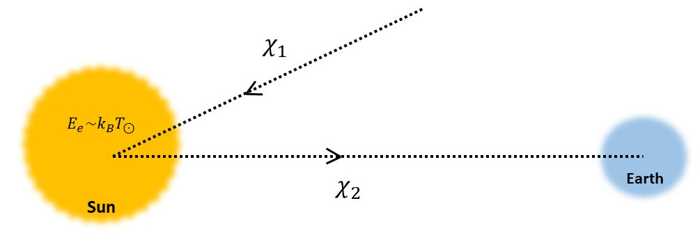
Figure 3: Direct detection of DM up-scattered in the Sun (adapted from An:2017ojc ).

In the following, we follow the discussion in refs. Baryakhtar:2020rwy ; An:2017ojc ; Emken:2021lgc to find the event rates at DD experiments.

III.1 Up-scattering from the Sun

The maximum velocity of DM falling into the Sun is $\sqrt{(v^{\rm{esc}}_{\odot})^{2}+(v_{\rm{DM}}^{\rm{\,halo}})^{2}}\simeq 4\times 10^{-3}$, where $v^{\rm{esc}}_{\odot}$ is the Solar escape velocity. We take the value of the Solar escape velocity to be the number averaged escape velocity, over the Solar core Emken:2021lgc (since most of the scatterings are expected to happen inside the core), giving $v^{\rm{esc}}_{\odot}\simeq\,1307\,\text{km/s}$ Emken:2021lgc . DM particle’s most probable Galactic velocity is given by $v_{DM}^{\textrm{halo}}\simeq 220\,\text{km/s}$. This is much smaller than the most probable electron velocity in the Solar core

$$v^{e}_{\odot}(\text{core})=\sqrt{\frac{2T_{\odot}}{m_{e}}}\simeq 0.066\text{, for }T_{\odot}=1.1\,\rm{keV},$$ (9)

where $T_{\odot}$ is the temperature at the Sun’s core. Hence, the DM particles can be understood to be at rest, with Solar electrons scattering against them. The steady state DM number density in the Sun is given by

$$n_{\chi_{1},\odot} =n_{\chi_{1}}^{\rm{\,halo}}\left(1+\left(\frac{v^{\text{esc}}_{\odot}}{v_{\text{DM}}^{\text{\,halo}}}\right)^{2}\right)\left(\frac{v_{\text{DM}}^{\text{\,halo}}}{v^{\rm{esc}}_{\odot}}\right)$$

$$\simeq n_{\chi_{1}}^{\rm{\,halo}}\left(\frac{v_{\rm{esc}}}{v_{\text{DM}}^{\text{\,halo}}}\right).$$ (10)

Here, the gravitational focusing effect, that enhances the area at spatial infinity, is given by the factor $(1+(v^{\text{esc}}_{\odot})^{2}/(v_{\text{DM}}^{\text{\,halo}})^{2})$, and the factor $(v_{\text{DM}}^{\text{\,halo}}/v_{\rm{esc}})$ accounts for the decrease in the number density of DM owing to its larger velocity near the Sun (from conservation of flux). The velocity distribution of electrons in the Sun is taken to be Maxwell Boltzmann (MB)

$$f_{{\rm MB}}(v_{e})=4\pi v_{e}^{2}\left(\frac{m_{e}}{2\pi T_{\odot}}\right)^{3/2}{\rm exp}\left(-\frac{m_{e}v_{e}^{2}}{2T_{\odot}}\right),$$ (11)

where $m_{e}$ and $v_{e}$ are the electron mass and velocity, respectively. The differential flux of particles $\chi_{2}$ generated with recoil energy $K_{\chi_{2}}$ is given as

$$\frac{d\Phi}{dK_{\chi_{2}}} = n_{e}\left\langle\frac{d\sigma_{\chi_{1}\rightarrow\chi_{2}}}{dK_{\chi_{2}}}v_{e}\right\rangle\frac{n_{\chi_{1},\odot}V_{\odot}}{4\pi(1{\rm AU})^{2}}$$ (12)

$$= \frac{n_{e}n_{\chi_{1},\odot}V_{\odot}}{4\pi(1{\rm AU})^{2}}\int_{v_{min}(K_{\chi_{2}})}^{\infty}dv_{e}\,f_{MB}\left(v_{e}\right)\frac{d\sigma_{\chi_{1}\rightarrow\chi_{2}}}{dK_{\chi_{2}}}\,v_{e}$$ (13)

$$= \begin{cases}\frac{n_{e}n_{\chi_{1},\odot}V_{\odot}}{4\pi(1{\rm AU})^{2}}\frac{\pi\alpha^{2}m_{e}^{2}}{\mu_{\chi e}^{2}}\frac{T_{\odot}}{m_{e}}\left(\frac{m_{e}}{2\pi T_{\odot}}\right)^{3/2}\bar{\sigma}_{e}\frac{1}{K_{\chi_{2}}}\text{exp}\left(-\frac{m_{e}}{4m_{\chi_{1}}T_{\odot}}\frac{(m_{\chi_{1}}K_{\chi_{2}}/\mu_{\chi e}+\delta)^{2}}{K_{\chi_{2}}}\right),\text{ EDM }\\ \frac{n_{e}n_{\chi_{1},\odot}V_{\odot}}{4\pi(1{\rm AU})^{2}}\left(\frac{m_{e}}{2\pi T_{\odot}}\right)^{1/2}\bar{\sigma}_{e}^{F_{DM}(q)=1}\frac{m_{\chi_{1}}}{\mu_{\chi e}^{2}}\,\text{exp}\left(-\frac{m_{e}}{4m_{\chi_{1}}T_{\odot}}\frac{(m_{\chi_{1}}K_{\chi_{2}}/\mu_{\chi e}+\delta)^{2}}{K_{\chi_{2}}}\right)\\ \qquad\times\Big{(}1+\frac{4m_{\chi_{1}}}{m_{\chi_{1}}-2m_{e}}\left(\frac{m_{e}^{2}}{4\mu_{\chi e}^{2}}+\frac{\delta m_{e}^{2}}{2\mu_{\chi e}m_{\chi_{1}}K_{\chi_{2}}}+\frac{m_{e}T_{\odot}}{m_{\chi_{1}}K_{\chi_{2}}}+\frac{m_{e}^{2}\delta^{2}}{4m_{\chi_{1}}^{2}K_{\chi_{2}}^{2}}\right)\Big{)},\text{ MDM,}\end{cases}$$ (14)

where $n_{e}=2\times 10^{25}\,\textrm{cm}^{-3}$ and $V_{\odot}=2.2\times 10^{31}\,\textrm{cm}^{3}$ are the Solar mean electron number density and volume, respectively Bahcall:2000nu ; Baryakhtar:2020rwy . The factor of $1/4\pi(1\textrm{AU})^{2}$ is the scaling in the flux on account of traveling from the Sun to the Earth, with the distance travelled being 1 AU (astronomical unit). The reduced mass is given by $\mu_{i,j}\equiv m_{i}m_{j}/(m_{i}+m_{j})$.

Here, we have plugged in the explicit expressions for the temperature averaged differential cross section for up-scattering, given by

$$\left\langle\frac{d\sigma_{\chi_{1}\rightarrow\chi_{2}}}{dK_{\chi_{2}}}v_{e}\right\rangle=\int_{v_{\rm min}}^{\infty}dv_{e}f_{\rm MB}(v_{e})\frac{d\sigma_{\chi_{1}\rightarrow\chi_{2}}}{dK_{\chi_{2}}}v_{e},$$ (15)

where $v_{\rm min}(K_{\chi_{2}})$ is the minimum velocity an electron must have in order to up-scatter a $\chi_{1}$ into a $\chi_{2}$, with recoil energy $K_{\chi_{2}}$, given as

$$v_{\rm min}=\frac{1}{\sqrt{2K_{\chi_{2}}m_{\chi_{1}}}}\left(\frac{m_{\chi_{1}}K_{\chi_{2}}}{\mu_{\chi_{1},e}}+\delta\right),$$ (16)

and

$$\frac{d\sigma_{\chi_{1}\rightarrow\chi_{2}}}{dK_{\chi_{2}}}\simeq\frac{\bar{\sigma}_{e}m_{\chi_{1}}}{2\mu_{\chi_{1},e}^{2}v_{e}^{2}}|F_{DM}(q)|^{2},$$ (17)

in the limit $\delta<<m_{e}$ and $m_{\chi_{1}}$. Here, $\bar{\sigma}_{e}$ is the DM-electron reference cross section Essig:2011nj with the 3-momentum transfer fixed at $q=(\alpha m_{e})$ (appropriate for atomic processes),

$$\bar{\sigma}_{e} \equiv\frac{\mu_{\chi_{1},e}^{2}}{16\pi m_{\chi_{1}}^{2}m_{e}^{2}}\overline{|\mathcal{M}_{\chi_{1}e}(q)|^{2}}\Big{|}_{q^{2}=(\alpha m_{e})^{2}}$$ (18)

$$=\begin{cases}\frac{4d_{\chi}2}{\alpha}\frac{m_{\chi_{1}}^{2}}{(m_{\chi_{1}}+m_{e})^{2}},\text{ with }F_{DM}(q)=\frac{\alpha m_{e}}{q},&\text{ for EDM,}\\ \left.\begin{array}[]{l}\alpha\mu_{\chi}^{2}\frac{m_{\chi_{1}}^{2}}{(m_{\chi_{1}}+m_{e})^{2}}\left(1-\frac{2m_{e}}{m_{\chi_{1}}}\right),\text{ with }F_{DM}(q)=1,\\ \frac{4}{\alpha}\mu_{\chi}^{2}v^{2}\frac{m_{\chi_{1}}^{2}}{(m_{\chi_{1}}+m_{e})^{2}},\text{ with }F_{DM}(q)=\frac{\alpha m_{e}}{q}.\end{array}\right\}&\text{ for MDM. }\end{cases}$$ (19)

The $q$-dependence of the matrix elements are encoded in the DM form-factor $F_{DM}(q)$ Essig:2011nj . $\overline{|\mathcal{M}_{\chi_{1}e}(q)|^{2}}$ is the squared-amplitude for DM–electron scattering, averaged (summed) over initial (final) spin states. The MDM contribution consists of one part that is independent of relative velocity $v$ and with a form factor $F_{DM}(q)=1$ similar to that for contact interaction, and another part proportional to $v^{2}$ and with a form factor same as that of EDM.

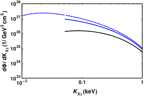
Figure 4: The differential flux of particles $\chi_{2}$ generated with recoil energy $K_{\chi_{2}}$, $\frac{d\Phi}{dK_{\chi_{2}}}$, at production (blue-dashed), the flux that escapes the Sun’s gravitational potential (blue-solid) and the attenuated flux at the Earth after taking into account $\chi_{2}$ decay in traveling from the Sun (black-solid).

Note that the $\chi_{2}$ particles that reach the Earth are the ones that overcome the gravitational potential well of the Sun,

$$v_{\chi_{2}}^{2}\simeq\frac{2K_{\chi_{2}}}{m_{\chi_{2}}}>(v^{\rm{esc}}_{\odot})^{2}.$$ (20)

Therefore, the flux on the Earth is attenuated from the produced flux as

$$\frac{d\Phi}{dK_{\chi_{2}}}(K_{\chi_{2}})\Bigg{|}_{Earth}=\frac{d\Phi}{dK_{\chi_{2}}}(K_{\chi_{2}}+m_{\chi_{2}}(v^{\rm esc}_{\odot})^{2}/2)\;\Theta\left(K_{\chi_{2}}-\frac{1}{2}m_{\chi_{2}}(v^{\rm{esc}}_{\odot})^{2}\right).$$ (21)

The Heaviside theta function ensures that the condition in eq. (20) is satisfied. We also shift the flux to account for the reduction in $\chi_{2}$ velocity in overcoming the Sun’s gravitational potential. In the following, we denote the flux on the Earth by $d\Phi/dK_{\chi_{2}}$ and drop the explicit notation. There will be a further suppression in the flux of $\chi_{2}$ from its decay in the time taken to travel from the Sun to the Earth. In fig. 4 we show the flux per unit energy from eq. (14) at production (blue-dashed), the flux that escapes the Sun’s gravitational well from eq. (21) (blue-solid) and the attenuated flux at the Earth after taking into account the $\chi_{2}$ decay in travelling from the Sun to the Earth (black-solid). Note that the flux that overcomes the gravitational potential has a lower cut-off, from the Heaviside theta function in eq. (21).

We note that the plasmon does not play any role in the up-scattering or production of DM in the Sun. The plasmon frequency in the non-relativistic limit Braaten:1993jw

$$\omega_{p}^{2}(T)=\frac{4\pi\alpha\,n_{e}}{m_{e}}\left(1-\frac{5}{2}\frac{T}{m_{e}}\right)$$ (22)

gives a plasmon mass order 1 smaller than the Sun’s average temperature for the Solar electron number density. Therefore, the plasmon effect is subdominant in scattering. In addition, there can be no plasmon-sourced production as we consider DM masses much larger than the Solar temperature.

III.2 Down-scattering on the Earth

III.2.1 Electron scattering:

The $\chi_{2}$ flux received on the Earth is depleted if the decay lifetime of $\chi_{2}$ is comparable to the time taken by it to travel to the Earth. We take this into account, and calculate the down-scattering event rate in electron scattering experiments. With the DM flux per unit energy $d\Phi/dK_{\chi_{2}}$ given in eq. (21), we can write the electron recoil energy spectrum per detector mass per unit time as Essig:2015cda ; Bloch:2020uzh ; Baryakhtar:2020rwy

$$\frac{dR_{\rm ion}}{d\Delta E_{e}} = n_{T}\,\epsilon(\Delta E_{e})\sum_{n,l}\frac{1}{\Delta E_{e}-E_{nl}}\frac{\bar{\sigma}_{e}}{64\mu_{\chi_{2},e}^{2}}\int dK_{\chi_{2}}\Theta(\Delta E_{e}^{\rm max}(K_{\chi_{2}})-\Delta E_{e})\frac{d\Phi}{dK_{\chi_{2}}}\frac{m_{\chi_{2}}}{K_{\chi_{2}}}e^{-t(K_{\chi_{2}})\times\Gamma_{\chi_{2}}}$$ (23)

$$\qquad\qquad\times\int_{q^{-}(K_{\chi_{2}},\Delta E_{e},\delta,m_{\chi_{2}})}^{q^{+}(K_{\chi_{2}},\Delta E_{e},\delta,m_{\chi_{2}})}dq\,q|F_{DM}(q)|^{2}|f_{nl\rightarrow\Delta E_{e}-E_{nl}}(q)|^{2},$$

where $\Delta E_{e}$ is the energy transferred to the electron, $E_{nl}$ is the ionization energy of the $n,\,l$ orbital of given atom, $\epsilon(\Delta E_{e})$ is the signal efficiency given in fig. 2 of  XENON:2020rca . The maximum energy transferred to the electron for a given incoming DM kinetic energy $K_{\chi_{2}}$ is given by $\Delta E_{e}^{\rm max}(K_{\chi_{2}})=K_{\chi_{2}}+\delta$. For DM-electron scattering in xenon, we get the number of targets per tonne as $n_{T}=2\times 4.2\times 10^{27}/\text{tonne}$. The exponential factor accounts for the depletion in $\chi_{2}$ flux in travelling from the Sun to the Earth and $t(K_{\chi_{2}})=1{\rm AU}\times\sqrt{m_{\chi_{2}}/2K_{\chi_{2}}}$ is the time taken by $\chi_{2}$ to travel to the Earth. The decay width of $\chi_{2}$ is,

$$\Gamma_{\chi_{2}}\simeq(d_{\chi},\mu_{\chi})^{2}\delta^{3}/\pi.$$ (24)

The form factor for ionization of an electron in $n,l$ orbital with a total of $\Delta E_{e}$ energy transferred to the electron, is given by $|f_{nl\rightarrow\Delta E_{e}-E_{nl}}(q)\big{|}^{2}$. We use QEDark Essig:2015cda to extract these ionization form factors.

The limits of integration $q^{\pm}$ are obtained from energy conservation in the down-scattering process and given as

$$\frac{q^{2}}{2m_{\chi_{2}}}-v\,q\,\textrm{cos}\,\theta=\delta-\Delta E_{e},$$ (25)

where $\theta$ is the angle between the momentum of $\chi_{2}$ and the transferred momentum $q$ and

$$|\textrm{cos}\,\theta|\leq 1\implies q^{\pm}(v,\Delta E_{e},\delta,m_{\chi_{2}})=\Big{|}m_{\chi_{2}}v\pm\sqrt{m_{\chi_{2}}^{2}v^{2}-2m_{\chi_{2}}(\Delta E_{e}-\delta)}\Big{|}.$$ (26)

We note that the factor from integration over transferred momentum $q$ in eq. (23)

$$f_{ion}^{int}(\Delta E_{e},q)=\int_{q^{-}(v,\Delta E_{e},\delta,m_{\chi_{2}})}^{q^{+}(v,\Delta E_{e},\delta,m_{\chi_{2}})}dq\,q\frac{\alpha^{2}m_{e}}{4(\Delta E_{e}-E_{nl})}|F_{DM}(q)|^{2}\big{|}f_{nl\rightarrow\Delta E_{e}-E_{nl}}(q)\big{|}^{2},$$

leads to an enhancement in the $F_{DM}(q)=1$ part of the MDM scattering rate but a small suppression for the remaining part of MDM as well as the EDM scattering rate.

We find the limits from latest results from XENONnT experiment XENONCollaboration:2022kmb with a total exposure of $1.16\,\textrm{tonne}\times\textrm{year}$ and background rate of $15.8\pm 1.3$  events$/(\textrm{tonne}\times\textrm{year}\times\textrm{keV})$. We also find the projected limits from future runs of XENONnT and DARWIN experiments, with projected exposures of $20\,{\rm tonne}\times{\rm year}$ and $200\,{\rm tonne}\times{\rm year}$, respectively. We use the same background rate for future projections, as that of the latest XENONnT run, to get the most conservative limits. We also use the same efficiency as of XENON1T, which gives a conservative bound, since the efficiency can only be expected to improve. We discuss the results in section V.

III.2.2 Scattering from Migdal effect:

In addition to the direct ionization of an electron, a DM particle scattering off of a nucleus can also lead to subleading electronic energy deposition into detectors via nuclear scattering. In a typical nuclear recoil the electron cloud is assumed to follow the recoiling nucleus instantaneously. But if the effect of the sudden acceleration of the nucleus, with the electron cloud still in its original position, is taken into account, it is known to deposit electronic energy via ionization/excitation of the recoiling atom (the Migdal effect) or the emission of a Bremsstrahlung photon migdal1941ionization ; Bernabei:2007jz ; Ibe:2017yqa ; XENON:2019zpr .

In the Migdal approximation, the whole electron cloud is assumed to recoil with the same velocity with respect to the nucleus, with no change in its shape. The rate for a nuclear scattering with recoil energy $E_{\rm NR}$ accompanied with a Migdal electron recoil with energy $E_{e}$ from $n,l$ orbital, leading to a deposition of total energy $\Delta E_{e}\simeq E_{e}+E_{nl}$, is Ibe:2017yqa ; Dolan:2017xbu ; Bell:2021zkr

$$\frac{d^{3}R}{dE_{\rm NR}dE_{e}dK_{\chi_{2}}}=\sum_{n,l}\frac{d^{2}R}{dE_{\rm NR}dK_{\chi_{2}}}\big{|}Z(E_{\rm det}-\mathcal{L}E_{\rm NR}-E_{nl})\big{|}^{2},$$ (27)

where, $E_{\rm det}=E_{e}+E_{nl}+\mathcal{L}E_{\rm NR}$. The Lindhard quenching factor is denoted by $\mathcal{L}$ and is the fraction of the nuclear recoil energy observed in the electron channel. Its value is well approximated to $\mathcal{L}\simeq 0.15$ Bell:2021zkr ; Essig:2015cda . The ionization form factor is given by $\big{|}Z(E_{\rm det}-\mathcal{L}E_{\rm NR}-E_{nl})\big{|}^{2}$ and its values for different orbitals are given in fig. 4 of ref. Ibe:2017yqa . The nuclear differential scattering rate is:

$$\frac{d^{2}R}{dE_{\rm NR}dK_{\chi_{2}}}=n_{T}\frac{d\Phi}{dK_{\chi_{2}}}\frac{d\sigma_{N}}{dE_{\rm NR}}e^{-t(K_{\chi_{2}})\times\Gamma_{\chi_{2}}}.$$ (28)

The nuclear differential scattering cross sections, approximated to the elastic case, are

$$\frac{d\sigma_{N}}{dE_{\rm NR}}\simeq\begin{cases}Z^{2}\alpha\frac{d_{\chi}^{2}}{16}\frac{1}{v^{2}E_{\rm NR}},&\textrm{for EDM,}\\ Z^{2}\alpha\frac{\mu_{\chi}^{2}}{16}\frac{1}{E_{\rm NR}}\left(1+\frac{E_{\rm NR}}{2\mu_{\chi_{2},N}v^{2}}\right),&\textrm{for MDM Spin Independent,}\\ \alpha\frac{\mu_{\chi}^{2}}{16}\left(\frac{\mu_{Z,N}}{e/2m_{N}}\right)^{2}\frac{m_{N}}{m_{n}^{2}v^{2}},&\textrm{for MDM Spin Dependent},\end{cases}$$ (29)

where $m_{N}$ and $Z$ are the mass and atomic number of the nucleus, respectively, and $E_{\rm NR}$ is the nuclear recoil energy.

The most sensitive low-energy analysis comes from the S2-only data set from the XENON1T experiment XENON:2019gfn . The S2-only differential rate is

$$\frac{dR}{dE_{\rm det}}=\int dE_{\rm NR}\int_{K_{\chi_{2}}^{min}}^{\infty}dK_{\chi_{2}}\frac{d^{3}R}{dE_{\rm NR}dE_{e}dK_{\chi_{2}}},$$ (30)

where the minimum kinetic energy of the incoming DM $\chi_{2}$ to downscatter to $\chi_{1}$, with a nuclear recoil energy of $E_{\rm NR}$ along with an electronic deposition of energy $E_{\rm det}$ via Migdal effect, is given by

$$K_{\chi_{2}}^{min} = \frac{m_{\chi_{2}}}{2}(v_{min}^{\rm Mig,inel})^{2},$$ (31)

$${\rm where,\,}v_{min}^{\rm Mig,inel} = \sqrt{\frac{m_{N}E_{\rm NR}}{2\mu_{\chi_{2},N}^{2}}}+\frac{\Delta E_{e}-\delta}{\sqrt{2m_{N}E_{\rm NR}}},$$ (32)

$$= \sqrt{\frac{m_{N}E_{\rm NR}}{2\mu_{\chi_{2},N}^{2}}}+\frac{E_{\rm det}-\mathcal{L}E_{\rm NR}-\delta}{\sqrt{2m_{N}E_{\rm NR}}}.$$ (33)

We find the total number of event at XENON1T by integrating eq. (30) over the range $E_{\rm det}=0.19-3.8$ keV_ee, with an exposure of 22 tonne-day XENON:2019gfn . A total of 61 events were observed at XENON1T over this exposure, while the expected number of background events was 23.4. This gives an upper limit of 49 events expected from DM at 90$\%$ confidence, and can be used as an upper limit to derive constraints on DM interactions with SM. For our model of dipolar DM though we find less than 1 events over the full parameter space of interest, so the scattering rate from Migdal effect is not large enough to derive any bounds on Solar upscattered dipolar DM.
We note that this is expected from the discussion in Essig:2019xkx for long range interactions, like EDM $F_{DM}(q)=1/q^{2}$, with a bias towards low $q$ values where the Migdal effect rates are always smaller than electron ionization rates by a factor of $\sim Z^{2}m_{e}^{2}/m_{N}^{2}$.

IV Complementary Bounds on sub-GeV Dark Matter

In this section, we discuss the constraints on sub-GeV DM with $\mathcal{O}$(keV) splittings from existing laboratory experiments and astrophysical sources.

IV.1 Fixed target experiments

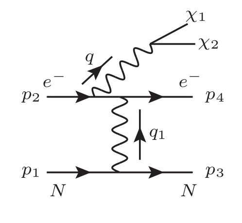
(a)

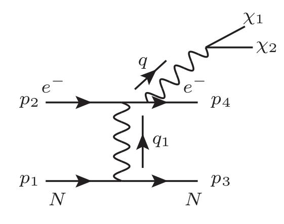
(b)

Figure 5: Leading processes for production of dark sector particles via off-shell photon in a fixed target experiment.

At lepton-fixed target experiments, an electron beam of fixed energy is dumped against an active target, comprised of some heavy nucleus, that is either a part of the detector itself or a separate target. Dark sector particles can be pair produced from the electrons scattering off of nucleons, giving rise to missing-energy final states Gninenko:2013rka ; Andreas:2013lya . These experiments employ stringent selection criteria making it possible to conduct an essentially background free search for such missing-energy signals Bjorken:2009mm ; Tsai:1973py ; Graham:2021ggy ; Fabbrichesi:2020wbt ; Agrawal:2021dbo .

In particular, we use results from the NA64 experiment at CERN SPS NA64:2017vtt to derive constraints on our model via the production of DM particles from an off-shell photon,

$$e^{-}N\rightarrow e^{-}N\gamma_{\rm vir}\rightarrow e^{-}N\chi_{1}\chi_{2},$$

where $\gamma_{\rm vir}$ is the off-shell photon that subsequently produces the dark sector particles. The leading processes are shown in fig. 5. Note that we do not consider the processes where the virtual photon originates from the nucleus since these processes are suppressed by a factor of $(Zm_{e}/m_{N})^{2}$ for coherent photon emission. We follow the discussion in ref. Chu:2018qrm in the following.

The NA64 experiment employs the optimized 100 GeV electron beam from the H4 beamline at the North Area (NA) of the CERN SPS. The beam is incident upon an electromagnetic calorimeter (ECAL) made up of a $6\times 6$ matrix with Pb and Sc plates, each module being $\simeq 40$ radiation lengths ($X_{0}$) long. The radiation length of Sc is about 1 order larger than that of Pb so $e^{-}$ scattering with Sc is subdominant.
Assuming that the fermion pair is produced within the first radiation length gives the target length to be $L_{\textrm{target}}=X_{0}=0.56\,$cm for Pb. The search region in the ECAL is limited by the energy threshold for detection of electron on one side and the requirement for missing energy to be larger than half the beam energy. This gives the selection criteria for the energy of the outgoing electron $E_{4}$ as Banerjee:2019pds ; Krasnikov:2020trl

$$0.3\,\textrm{GeV}<E_{4}<50\,\textrm{GeV}.$$ (34)

The polar angular coverage for the outgoing electron is

$$0.0<\theta_{4}<0.23\,\,{\rm radians}.$$ (35)

The number of signal events with these geometric and angular cuts are Chu:2018qrm

$$N_{\textrm{sig}}=N_{\textrm{EOT}}\frac{\rho_{\textrm{target}}}{m_{N}}L_{\textrm{target}}\int_{E_{4}^{min}}^{E_{4}^{max}}\epsilon_{eff}(E_{4})\int_{\textrm{cos}\,\theta_{4}^{min}}^{\textrm{cos}\,\theta_{4}^{max}}d\textrm{cos}\,\theta_{4}\frac{d\sigma_{\textrm{prod}}}{dE_{4}d\textrm{cos}\,\theta_{4}},$$ (36)

where, $N_{\textrm{EOT}}=2.84\times 10^{11}$ are the number of electrons incident upon the target Banerjee:2019pds . The target material density and nuclear mass are given by $\rho_{\rm target}$ and $m_{N}$, respectively. The detector efficiency of NA64 is known to depend only marginally on the energy and is taken to be constant, $\epsilon_{eff}(E_{4})\simeq 0.5$ (averaging over the total signal efficiencies of the various runs Banerjee:2019pds ). The integration limits of $E_{4}$ and $\theta_{4}$ are from eqs. (34) and (35), respectively. The double differential cross section for production of the processes shown in figs. 5(a) and 5(b) is given by $d\sigma_{prod}/dE_{4}d\cos\theta_{4}$ with the full expression given in eq. (82).

Since the beam energy is much larger than the $\mathcal{O}$(keV) splitting we consider, and the signal being observed is of missing energy in final state, the constraints on our model do not differ from those of the elastic DM cases discussed in ref. Chu:2018qrm . We follow the discussions in Chu:2018qrm and re-derive the constraints from their run as mentioned in ref. Banerjee:2019pds . The details of the calculation are given in Appendix C. We derive constraints by demanding that $N_{sig}<N^{90\%}=2.3$ where the latter corresponds to the $90\%$ C.L. for the number of signals events given zero observed events. The resulting constraints are shown in figs. 7 and 11.

This type of search for missing-energy in the final state gives stronger bounds for a feebly interacting dark particle, as compared to experiments where the dark particle is detected via its scattering off electrons/nuclei in the main detector (for example in the mQ experiment at SLAC Prinz:1998ua ), since processes of the latter kind are suppressed by further powers of the small-valued DM-SM effective coupling. We, therefore, do not study these latter processes.

Constraints are also derived from proton fixed target experiments, and as shown in ref. Chu:2020ysb the strongest such constraint comes from CHARM-II experiment, which used a 450 GeV proton beam on a Be target. The constraints are derived from single electron recoil events at recoil energies $E_{R}\in[3,24]$ GeV, so that the small splitting of $\mathcal{O}$(keV) has negligible effect and the constraints for such inelastic DM are the same as those for the elastic case. These are shown in figs. 7 and 11.

IV.2 Production at lepton colliders

DM can be produced from $e^{+}e^{-}$ collisions at lepton colliders and appear as missing energy ($\not{E}$), since they do not scatter within the collider. Along with initial state radiation (ISR) or final state radiation (FSR), this leads to a particularly clean signature of mono-photon plus missing energy ($\gamma+\not{E}$). The FSR processes are suppressed by the small DM-photon couplings, so we only consider the ISR process, as shown in fig. 6, for deriving constraints.

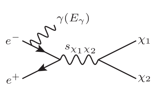
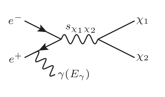
Figure 6: Processes for production of DM along with initial state radiation, at $e^{+}e^{-}$ colliders, leading to missing energy plus mono-photon signatures.

We follow the discussion in ref. Chu:2019rok for constraints on DM dipole moments from pair production, adapting them for the inelastic case. For DM mass splittings much smaller than the CM energy of the $\chi_{1},\chi_{2}$ system, $\delta\sim\mathcal{O}(\text{keV})<<\sqrt{s_{\chi_{1}\chi_{2}}}$, these constraints for inelastic DM are equal to the ones for elastic DM.

IV.2.1 BABAR

We use the data from the search for mono-photon events in decays of $\Upsilon(3S)$

$$\Upsilon(3S)\rightarrow\gamma(A^{0}\rightarrow inv.)$$

at BABAR detector at the PEP-II asymmetric-energy $e^{+}e^{-}$ collider at the Stanford Linear Accelerator Center (SLAC), with 28 fb^-1 of data collected at a CM energy BaBar:2008aby

$$\sqrt{s}\approx m_{\Upsilon(3S)}\approx\,10.355\,\textrm{GeV.}$$

The single-photon events were chosen based one two trigger criteria,

High-E region: $$3.2<E_{\gamma}<5.5\,\textrm{GeV,\,}-0.31<\textrm{cos}\,\theta_{\gamma}<0.6\,\,{\rm radian}, \textrm{full data},$$

Low-E region: $$2.2<E_{\gamma}<3.7\,\textrm{GeV,\,}-0.46<\textrm{cos}\,\theta_{\gamma}<0.46\,\,{\rm radian}, \textrm{19\,fb${}^{-1}$ of data},$$

where $\theta_{\gamma}$ is the CM polar angle, and $E_{\gamma}$ is the photon energy in the $\Upsilon$ rest frame. For each region, the number of signal events is given by

$$N_{sig}^{(i)}=\epsilon_{\text{eff}}\,\mathcal{L}\int_{\text{bin }i}\frac{ds_{\chi_{1}\chi_{2}}}{s}\int_{\textrm{cos}\,\theta_{\gamma}^{\text{min}}}^{\textrm{cos}\,\theta_{\gamma}^{\text{max}}}d\,\textrm{cos}\,\theta_{\gamma}\frac{d\sigma_{e^{+}e^{-}\rightarrow\chi_{1}\chi_{2}\gamma}}{dx_{\gamma}d\textrm{cos}\,\theta_{\gamma}}.$$ (37)

Here, $\epsilon_{\text{eff}}$ is the total efficiency, $\mathcal{L}$ is the integrated luminosity, $\sqrt{s}$ is the CM energy of the $e^{+}e^{-}$ system, $\sqrt{s_{\chi_{1}\chi_{2}}}\equiv\sqrt{(1-x_{\gamma})s}$ is the CM energy of the $\chi_{1}\chi_{2}$ system with $x_{\gamma}=E_{\gamma}/E_{beam}=2E_{\gamma}\big{/}\sqrt{s}$. The photon makes an angle of $\theta_{\gamma}$ with respect to the beam in the CM frame. Following ref. Essig:2013vha we apply a non-geometric cut $\epsilon_{\text{eff}}$ of $30\%$ and $55\%$ in the high-E and low-E regions, respectively.

The ISR production cross section is approximated by dressing the cross section for DM pair production (without ISR), with an angle-dependent radiator function Montagna:1995wp ; Chu:2019rok as:

$$\frac{d\sigma_{e^{+}e^{-}\rightarrow\chi_{1}\chi_{2}\gamma}}{dx_{\gamma}d\textrm{cos}\,\theta_{\gamma}}=\sigma_{e^{+}e^{-}\rightarrow\chi_{1}\chi_{2}}(s,s_{\chi_{1}\chi_{2}})\mathcal{H}^{(\alpha)}(x_{\gamma},\theta_{\gamma},s),$$ (38)

where the cross-section for $e^{+}e^{-}\rightarrow\chi_{1}\chi_{2}$ at the energy scale reduced by photon emission is

$$\sigma_{e^{+}e^{-}\rightarrow\chi_{1}\chi_{2}} =\frac{1}{32\pi\sqrt{s\,s_{\chi_{1}\chi_{2}}}}\frac{|\vec{p}_{f}|}{|\vec{p}_{i}|}\int d(\textrm{cos}\,\theta)\,\overline{|\mathcal{M}|^{2}}$$ (39)

$$=\frac{\alpha(s+2m_{e}^{2})}{6s_{\chi_{1}\chi_{2}}^{3}}\sqrt{\frac{m_{\chi_{1}}^{4}-2m_{\chi_{1}}^{2}(m_{\chi_{2}}^{2}+s_{\chi_{1}\chi_{2}})+(m_{\chi_{2}}^{2}-s_{\chi_{1}\chi_{2}})^{2}}{s(s-4m_{e}^{2})}}$$

$$\quad\times\begin{cases}d_{\chi}^{2}\Big{(}s_{\chi_{1}\chi_{2}}^{2}+s_{\chi_{1}\chi_{2}}(m_{\chi_{1}}^{2}-6m_{\chi_{1}}m_{\chi_{2}}+m_{\chi_{2}}^{2})-2\,(m_{\chi_{2}}^{2}-m_{\chi_{1}}^{2})^{2}\Big{)},&\text{for EDM},\\ \mu_{\chi}^{2}\Big{(}s_{\chi_{1}\chi_{2}}^{2}+s_{\chi_{1}\chi_{2}}(m_{\chi_{1}}^{2}+6m_{\chi_{1}}m_{\chi_{2}}+m_{\chi_{2}}^{2})-2\,(m_{\chi_{2}}^{2}-m_{\chi_{1}}^{2})^{2}\Big{)},&\text{for MDM},\\ \end{cases}$$ (40)

and, the radiator function taking into account all soft and collinear corrections upto $\mathcal{O}(m_{e}^{2}/s)$ is  Montagna:1995wp

$$H^{\alpha}(x_{\gamma},\theta_{\gamma},s)=\frac{\alpha}{\pi}\frac{1}{x_{\gamma}}\left[\frac{1+(1-x_{\gamma})^{2}}{1+4m_{e}^{2}/s-\textrm{cos}^{2}\theta_{\gamma}}-\frac{x_{\gamma}^{2}}{2}\right].$$ (41)

To constrain the DM couplings, we require that the expected number of events be smaller than the observed number of events in each bin $i$ at 90$\%\,$C.L., such that $N_{sig}^{(i)}<N_{obs}^{(i)}+1.28\,\sigma_{obs}^{(i)}$. We show these bounds in figs. 7 and 11.

IV.2.2 LEP

We consider high energy colliders like the Large Electron Positron (LEP) collider. The model considered here can give rise to events with one photon and missing energy by the same process as at BABAR, see section IV.2.1. The only difference lies in the high CM energies $189\,\textrm{GeV}\leq\sqrt{s}\leq 209\,$GeV and high luminosities (a total of $619$ pb^-1 of data for the single- and multi-photon $+$ missing energy final states) that the LEP operated at L3:2003yon . The cross sections for these processes having been found to be in agreement with the SM expectation from $e^{+}e^{-}\rightarrow\nu\bar{\nu}\gamma(\gamma)$ give constraints on any BSM physics model that can also lead to the same final state. But the high CM energies lead to constraints that are independent of the DM mass, for light DM ($m_{\chi}<$ GeV here). This was studied in ref. Fortin:2011hv and bounds obtained from the mono photon channels give

$$|\mu_{\chi}|\textrm{\,or\,}|d_{\chi}|<1.3\times 10^{-5}\mu_{B},$$ (42)

where $\mu_{B}\equiv e/2m_{e}$ is the Bohr magneton. We note that at these large energies of production, the small splitting of $\mathcal{O}$(keV) has negligible effect and the constraints for such inelastic DM are the same as those for the elastic case. The upper bound is shown in figs. 7 and 11.

Note that the LHC probes heavier masses and smaller couplings $\sim\mathcal{O}(0.01)$ GeV^-1 Barger:2012pf , and is not of relevance in this work.

IV.3 Supernovae cooling

Light DM, $m_{DM}\leq\mathcal{O}(100\textrm{\,MeV}$), can be produced in supernovae with core temperatures of $\mathcal{O}$(30 MeV) Raffelt:1996wa ; Dreiner:2003wh ; Fischer:2016cyd ; Magill:2018jla ; Chang:2016ntp ; Chang:2018rso . If these dark particles escape, they can cause extra cooling and lead to changes in the shape and duration of the neutrino pulse. Light dark particles can thus be constrained by comparing neutrino pulse predictions to those observed from the SN1987A at terrestrial neutrino observatories Kamiokande-II:1987idp ; Bionta:1987qt ; Alekseev:1988gp , assuming that the SN1987A was a neutrino-driven supernova (SN) explosion Chu:2019rok . The constraints derived from SN depend on their cooling rate, with the predominant process being

$$e^{+}(p_{1}),e^{-}(p_{2})\rightarrow\chi_{1}(p_{3}),\chi_{2}(p_{4})$$ (43)

since positrons are thermally supported in SN. Constraints on models are derived in two limiting cases leading to two-sided bounds on DM couplings for each mass as follows:

1. Weak coupling: This is applicable in the limit of small interaction strengths of DM with SM such that for any smaller strengths there would be too little production of DM to cause any significant change to the SN cooling rate. In this limit, any DM that is produced escapes the SN with almost $100\%$ probability, such that it is possible to derive lower bounds on the DM effective coupling, by constraining only the production rates. This is given by the “Raffelt criterion” Raffelt:1996wa which says that any “exotic” cooling will not change the neutrino signal significantly, as long as the emissivity obeys the condition

   $$\dot{\mathcal{E}}<10^{19}\,\textrm{erg/g/s}.$$ (44)

   This condition is easily converted into a condition on energy emitted per unit time per unit volume by noting that the density for $t\simeq 1\textrm{s}$ is nearly constant (see fig. 5 of ref. Burrows:1986me ), giving a conversion between $d^{3}r$ and $dM$. We take $\rho\approx 3\times 10^{14}\,\textrm{g/cm}^{3}$. The emissivity (energy emitted per unit volume per unit time) is defined as Dreiner:2003wh

   $$\frac{d\mathcal{E}}{dt} =\int d\Pi_{i=1,4}\frac{d^{3}p_{i}}{(2\pi)^{3}(2E_{i})}(2\pi)^{4}\delta^{4}(p_{1}+p_{2}-p_{3}-p_{4})f_{1}f_{2}(1-f_{3})(1-f_{4})|\mathcal{M}|^{2}(E_{3}+E_{4}),$$ (45)

   where $f_{i}$ are the Fermi-Dirac distribution functions

   $$f_{i}\equiv\frac{1}{\textrm{exp}\left(\frac{E_{i}-\mu_{i}}{T}\right)+1}.$$ (46)

   We ignore the final state Pauli blocking for small DM number densities and simplify the expression using

   $$\int d\Pi_{i=1,2}\frac{d^{3}p_{i}}{(2\pi)^{3}(2E_{i})}(2\pi)^{4}\delta^{4}(p_{1}+p_{2}-p_{3}-p_{4})f_{1}f_{2}(1-f_{3})(1-f_{4})|\mathcal{M}|^{2}(E_{3}+E_{4})$$

   $$\quad\simeq(E_{1}+E_{2})f_{1}f_{2}\times 4v_{m\textrm{\o}l}E_{1}E_{2}\sigma^{\prime}$$ (47)

   $$\quad=(E_{1}+E_{2})f_{1}f_{2}\times 4F\sigma^{\prime},$$ (48)

   where we use energy conservation $E_{1}+E_{2}=E_{3}+E_{4}$ and $F\equiv\left(\sqrt{s(s-4m_{e}^{2})}/2\right)$ Gondolo:1990dk . The cross-section of production for the process in eq. (43) with squared-amplitude summed over initial and final spins, is given in the limit of vanishing electron mass $m_{e}^{2}<s\approx T_{avg}^{2}\simeq(30\,\textrm{MeV})^{2}$ as

   $$\sigma^{\prime} =\frac{2\alpha}{3s^{2}}\sqrt{\frac{m_{\chi_{1}}^{4}-2m_{\chi_{1}}^{2}\left(m_{\chi_{2}}^{2}+s\right)+\left(m_{\chi_{2}}^{2}-s\right)^{2}}{s^{2}}}$$

   $$\qquad\times\begin{cases}d_{\chi}^{2}\left(s(m_{\chi_{1}}^{2}-6m_{\chi_{1}}m_{\chi_{2}}+m_{\chi_{2}}^{2})-2(m_{\chi_{1}}^{2}-m_{\chi_{2}}^{2})^{2}+s^{2}\right),&\text{for EDM},\\ \mu_{\chi}^{2}\left(s(m_{\chi_{1}}^{2}+6m_{\chi_{1}}m_{\chi_{2}}+m_{\chi_{2}}^{2})-2(m_{\chi_{1}}^{2}-m_{\chi_{2}}^{2})^{2}+s^{2}\right),&\text{for MDM.}\\ \end{cases}$$ (49)

   Also simplifying the remaining part of eq. (45) as Gondolo:1990dk ; Dutra:2019gqz

   $$\int\frac{d^{3}p_{1}}{(2\pi)^{3}(2E_{1})}\frac{d^{3}p_{2}}{(2\pi)^{3}(2E_{2})}=\frac{1}{8(2\pi)^{4}}\int ds\int_{\sqrt{s}}^{\infty}dE_{+}\,E_{+}\int_{-\sqrt{E_{+}^{2}-s}}^{\sqrt{E_{+}^{2}-s}}dE_{-},$$ (50)

   with $E_{\pm}\equiv E_{1}\pm E_{2}$, we rewrite eq. (45) in the limit of vanishing electron mass as

   $$\frac{d\mathcal{E}}{dt}=\frac{1}{4(2\pi)^{4}}\int_{(m_{\chi_{1}}+m_{\chi_{2}})^{2}}^{\infty}ds\,s\,\sigma^{\prime}(s)\int_{\sqrt{s}}^{\infty}dE_{+}E_{+}\int_{E_{-}^{min}}^{E_{-}^{max}}dE_{-}f_{1}f_{2}$$ (51)

   where

   $$f_{1,2}=\frac{1}{\textrm{exp}\left(\frac{E_{+}\pm E_{-}\mp 2\mu_{e}(r_{0})}{2T(r_{0})}\right)+1},$$

   computed at radius $r_{0}=10$ km, where the emmissivity can be seen to be maximum. We use the temperature and chemical potential radial profiles as given in ref. Magill:2018jla . The limits of $E_{-}$ integration are $E_{-}^{max,min}\equiv\pm\sqrt{1-4m_{e}^{2}/s}\sqrt{E_{+}^{2}-s}$.

2. Large coupling: In the opposite limit of large DM couplings, the cooling process is dictated by the probability of escape or mean free path (MFP) of DM. The relatively larger density of SN results in a trapping of DM particles produced inside the SN, giving an upper bound on the DM effective coupling with SM. We adapt this bound from ref. Chu:2018qrm , shown in figs. 7 and 11.

V Results

We summarise the results for sub-GeV pseudo-Dirac DM with mass states $\chi_{1}$ and $\chi_{2}$ having mass difference $\mathcal{O}$(keV) for the two interactions:

1. Transition EDM interaction:

   • As discussed in section II.1, the FI production is UV sensitive. We show the relic density contours for two reheating temperatures, 5 MeV and 10 MeV, in fig. 7. For higher values of reheating temperatures, the contours would shift to lower $d_{\chi}$ values and the upward bend would occur at higher $m_{\chi_{1}}$, going outside the range shown here. The $T_{RH}=5\,{\rm MeV}$ contour can be seen to cut off at $m_{\chi_{1}}\simeq 100\,{\rm MeV}$ as the observed relic density cannot be reproduced via FI production for larger masses. We show the relic contours for two values of mass splittings, $\delta=1\,{\rm keV}$ (dashed) and $\delta=10\,{\rm keV}$ (dotted). These coincide at small masses for a given reheating temperature, since $\delta<<m_{\chi_{1}}$. But they begin to diverge for larger masses, $m_{\chi_{1}}\gtrsim T_{RH}$, as the Boltzmann suppression leads to an exponential that is more sensitive to the difference of the two masses.
     We can see that the bounds from SN1987A are applicable on parts of these contours.

   • The total number of events at various xenon based DD experiments are shown in the color palette in fig. 7. The points shown correspond to a mass splitting of $\delta=1\,\text{keV}$. We find that masses less than 12 MeV and $4\times 10^{-6}\,{\rm GeV}^{-1}\lesssim d_{\chi}\lesssim 10^{-5}\,{\rm GeV}^{-1}$ are ruled out by XENONnT. These results are to be understood to be correct upto $\mathcal{O}(10\%)$ since we ignore astrophysical uncertainties (solar parameters and DM halo distribution) in probing orders of magnitude of DM masses.

     

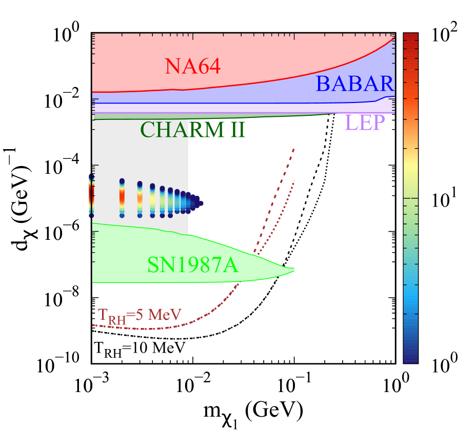
     (a) XENONnT

     

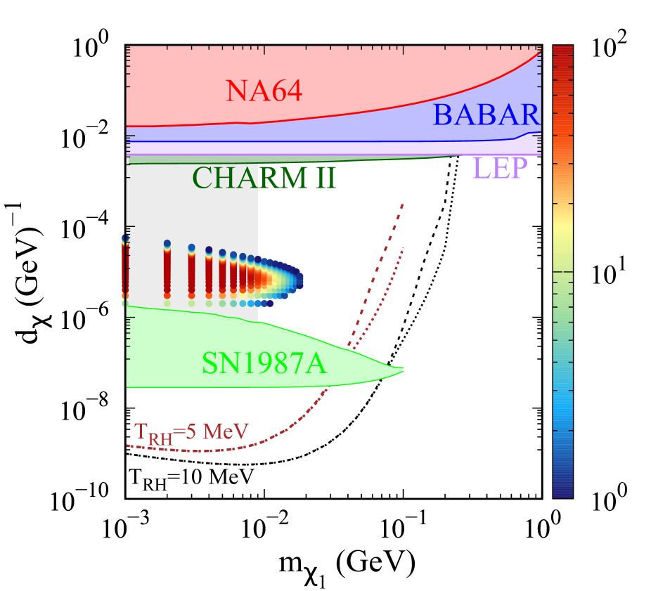
     (b) XENONnT projection

     

     (c) DARWIN

     Figure 7: Constraints (shaded regions) on the transition electric dipole moment (EDM) from NA64 (red), BABAR (blue), LEP (purple), CHARM-II (dark green) and SN1987A (green). The gray shaded region is ruled out by $N_{\rm eff}$ constraints in standard cosmology Chang:2019xva . Also shown are the contours that lead to observed relic density for $T_{RH}=$ 5 MeV (brown) and 10 MeV (black). The dashed and dotted lines for each correspond to mass splittings of $\delta=$ 1 keV and 10 keV, respectively. The points with color palette show the total number of events for mass splitting $\delta=1\,\text{keV}$ for various xenon experiments, as mentioned below each figure.

   • We note that there is a competition between the decay rate of $\chi_{2}$ and its down-scattering cross section at DD experiments. This is because increasing $d_{\chi}$ gives larger scattering cross sections as seen from eq. (19), but also increases the decay width, $\Gamma_{\chi_{2}}\propto d_{\chi}^{2}$, so that the flux received on the Earth decreases. Therefore, we see from fig. 7 that starting from the smallest values of $d_{\chi}$, the rate initially increases with increasing $d_{\chi}$, maximizing at some value of $d_{\chi}$ and then falls quickly with further increase in $d_{\chi}$.

   • This competition also leads to a maximum DM mass that can be probed at DD experiments. The XENONnT experiment currently probes masses $m_{\chi_{1}}\lesssim$12 MeV, while in the future XENONnT can probe $m_{\chi_{1}}\lesssim 18\,$MeV and DARWIN can probe $m_{\chi_{1}}\lesssim 23\,$MeV. We note that a large part of the points probed by XENONnT lie in the parameter space ruled out by $N_{\rm eff}$ bounds Chang:2019xva for this model. These arise because of thermalization of the dark sector for large enough couplings, assuming standard cosmology.

   • Larger parts of the parameter space that aren’t ruled out by $N_{\rm eff}$ bounds will be probed by future runs of XENONnT and DARWIN. Further, we show the event shapes for some benchmark points in figs. 8, 9 and 10, showing in red the signal+background rates, and the blue band corresponds to background rates with Poissonian uncertainties ($\pm\sqrt{N}$). We see that the signals may show up as an excess in the lowest recoil energy bins, and can also be distinguished from the background by the shape of the spectra.

     We can see the decrease in event rates when $\delta$ is increased from 1 keV in fig. 8 to 1.5 kev in fig. 10. This is because as $\delta$ increases, the decay width of $\chi_{2}$ increases, $\Gamma_{\chi_{2}}\propto\delta^{3}$. In addition, the up-scattering rates in the Sun get suppressed since the only electrons with enough energy to cause the up-scattering are those from the high velocity tail of MB distribution, given an average temperature of $T_{\odot}\simeq 1.1$ keV. Together, these prohibit the detection of large mass splittings ($\delta\gtrsim 1.2$ keV at XENONnT current run, $\delta\gtrsim 1.7$ keV at XENONnT future projection and $\delta\gtrsim 1.8$ keV at DARWIN) via electron scattering.

   • The minimum $d_{\chi}$ values that can be probed by DD experiments are such that the parameter space that leads to the production of observed relic density by FI production, is not within the reach of the DD experiment. While smaller reheating temperatures could lead to an overlap between the two, its value is bounded from below by $T_{RH}>4$ MeV Hannestad:2004px .

   • We also show the complementary bounds from other experiments/ observations (NA64, BaBar, LEP and SN cooling) in fig. 7 for completeness.

   

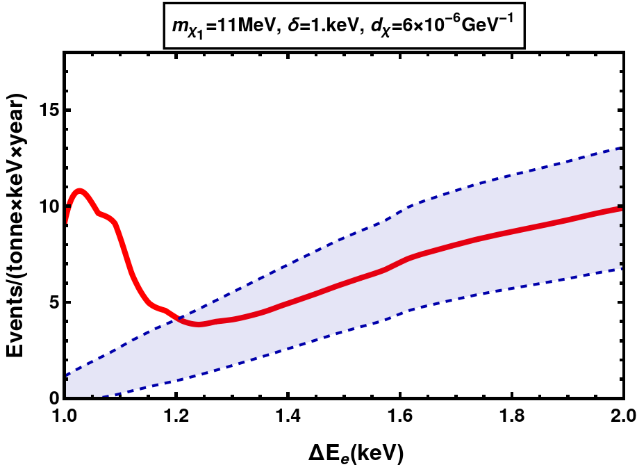
   (a) $m_{\chi_{1}}=11$ MeV, $\delta=1\,$keV at XENONnT

   

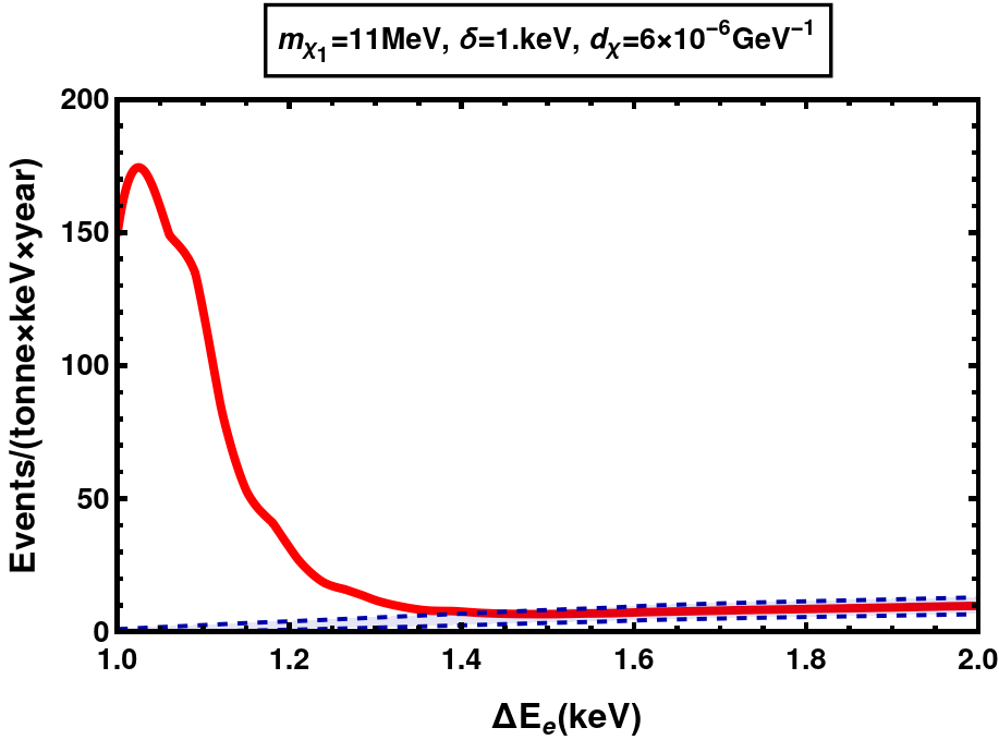
   (b) $m_{\chi_{1}}=11$ MeV, $\delta=1\,$keV at XeNONnT (proj.)

   

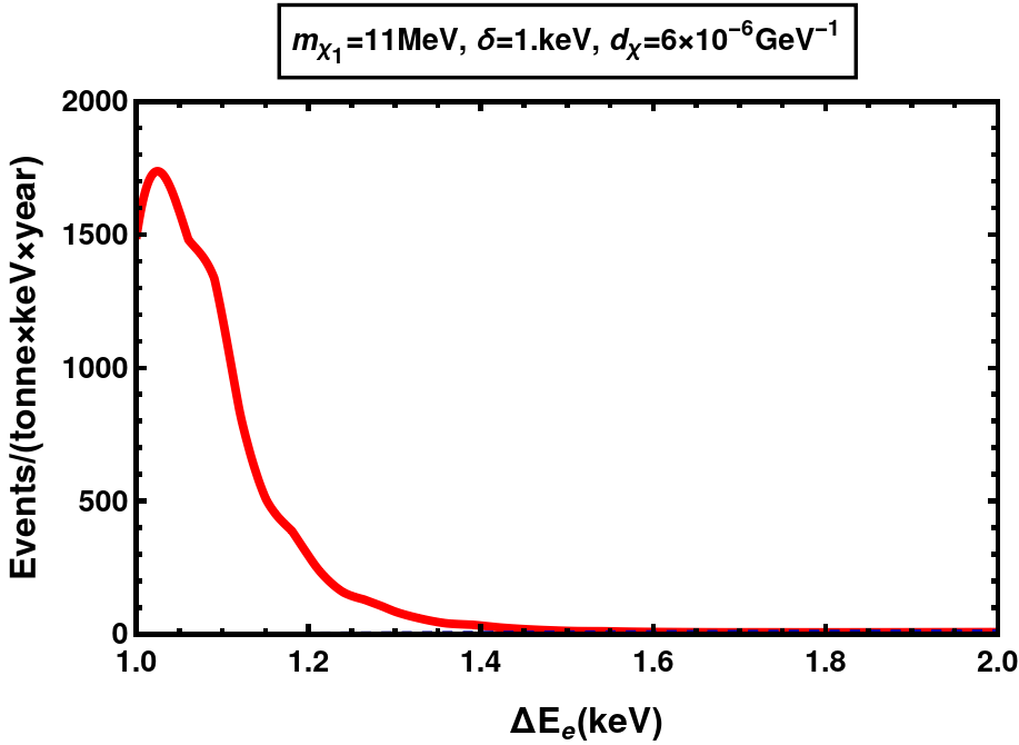
   (c) $m_{\chi_{1}}=11$ MeV, $\delta=1\,$keV at DARWIN

   Figure 8: Differential event rates for EDM DM with $\delta=1.0$ keV. Shown in blue are the background rates with the band representing Poissonian $(\pm\sqrt{N})$ uncertainties and in red are the signal+background rates.

   

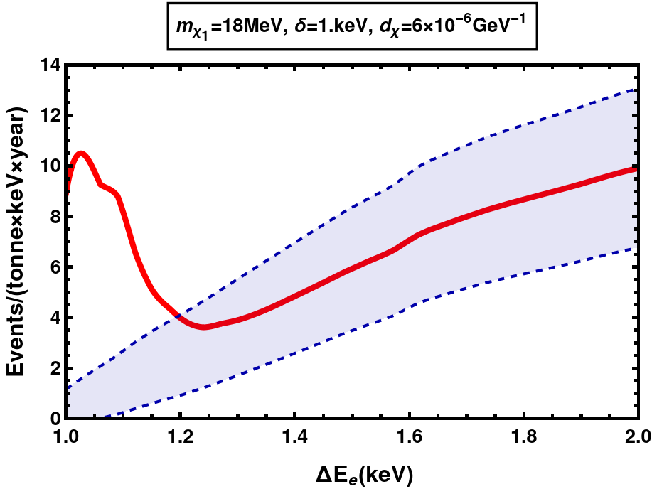
   (a) $m_{\chi_{1}}=18$ MeV, $\delta=1\,$keV at XENONnT (proj.)

   

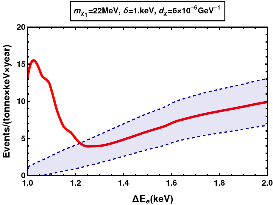
   (b) $m_{\chi_{1}}=22$ MeV, $\delta=1\,$keV at DARWIN

   Figure 9: Differential event rates for EDM DM with $\delta=1.0\,$keV. Shown in blue are the background rates with the band representing Poissonian $(\pm\sqrt{N})$ uncertainties and in red are the signal+background rates.

   

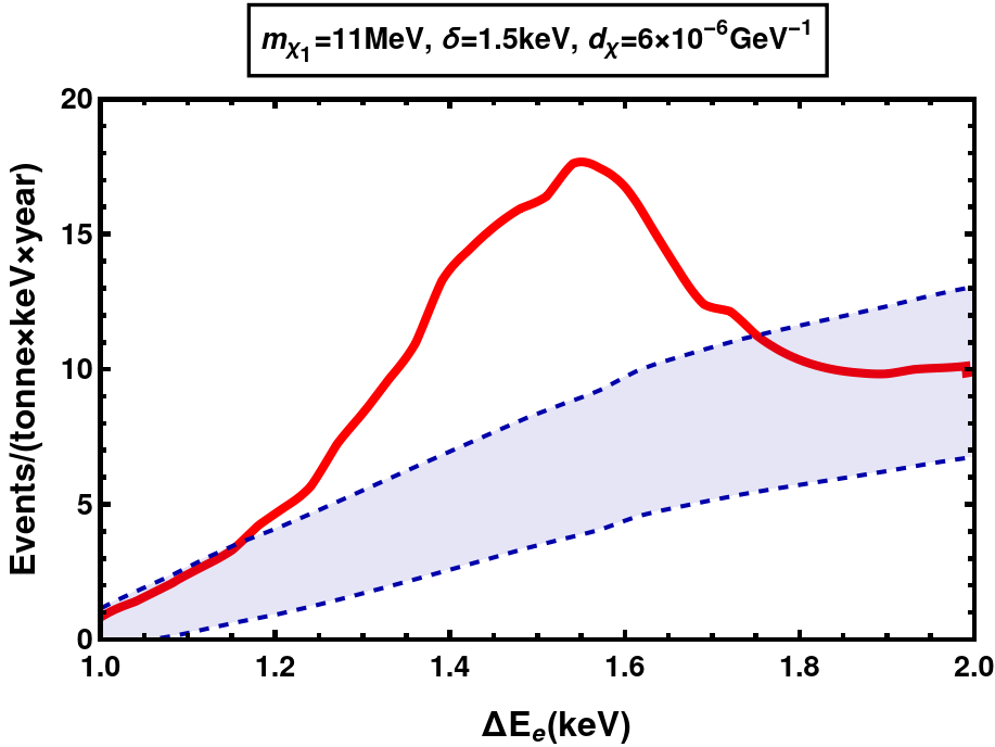
   (a) $m_{\chi_{1}}=11{\rm MeV}$, $\delta=1.5{\rm keV}$ at XENONnT (proj.)

   

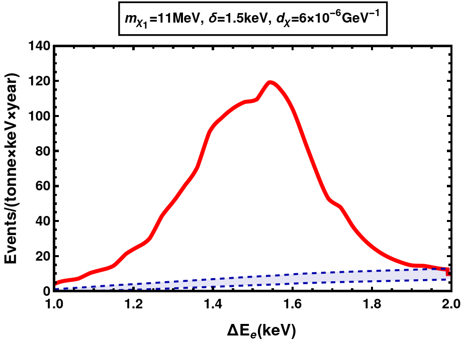
   (b) $m_{\chi_{1}}=11$ MeV, $\delta=1.5\,$keV at DARWIN

   Figure 10: Differential event rates for EDM DM with $\delta=1.5\,$keV. Shown in blue are the background rates with the band representing Poissonian $(\pm\sqrt{N})$ uncertainties and shown in red are the signal+background rates.

   

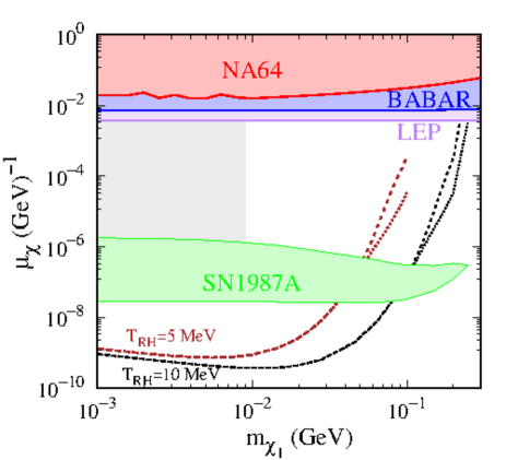
   Figure 11: Constraints (shaded regions) on the transition magnetic dipole moment (MDM) from NA64 (red), BABAR (blue), LEP (purple), CHARM-II (dark green) and SN1987A (green). The gray shaded region is ruled out by $N_{\rm eff}$ constraints in standard cosmology Chang:2019xva for this model. These arise because of thermalization of the dark sector for large enough couplings, assuming standard cosmology. Also shown are the contours that lead to observed relic density for $T_{RH}=$ 5 MeV (brown) and 10 MeV (black). The dashed and dotted lines for each correspond to mass splittings of $\delta=$ 1 keV and 10 keV, respectively.

2. Transition MDM interaction:
   Here, we only discuss the features that are distinct from the EDM case, with all other features being the same.

   • We note from eqs. (17) and (19) that the MDM differential cross section $d\sigma/dE_{R}\propto\{v^{2}/E_{R},1\}$ (corresponding to the two form factors $F_{DM}=1,1/q$, see eq. (19)) which is suppressed with respect to the corresponding EDM $d\sigma/dE_{R}\propto 1/v^{2}E_{R}$ by factors of $\{v^{4},v^{2}E_{R}\}$. Here we use the fact that $q^{2}\simeq 2m_{e}E_{R}$ and the suppression comes from $v$ and $E_{R}$ being small. Therefore, the scattering rates for MDM interaction are highly suppressed and do not lead to significant event rates at the xenon DD experiments, thus are not shown in fig. 11.

VI Conclusions and Outlook

We have studied a model of inelastic DM interacting with SM via transition electric and magnetic dipole moments. We first address the production of DM by the FI mechanism taking into account both $2\rightarrow 2$ annihilation production and production from decay of plasmon. We find that both these processes are UV dominant with the rate of production (or $dY/dT$) maximised at the largest temperatures (near $T_{RH}$). We observe that the plasmon production is insignificant for the parameter space we are interested in here, although it can become the dominant source of production for much larger reheating temperatures.

The heavier states are not stable on cosmological scales and their flux is produced by Solar up-scattering of the lighter, stable $\chi_{1}$ particles that are assumed to make up the entirety of DM. We study the constraints on this model from DD experiments where we can observe the down-scattering of the heavier mass state in electron recoil events. We find that DM with masses less than 12 MeV and transition EDM $4\times 10^{-6}\,{\rm GeV}^{-1}\lesssim d_{\chi}\lesssim 10^{-5}\,{\rm GeV}^{-1}$ are ruled out by XENONnT XENONCollaboration:2022kmb , already probing parameter space not ruled out by any other constraints.

In addition, we find that future results from DD experiments, XENONnT and DARWIN, by virtue of larger exposures and lower backgrounds, can lead to the discovery of pseudo-Dirac DM with EDM interaction and mass splittings less than 2 keV. Notably, this parameter space is not probed by any current experiment. The reach of DD experiments will further improve by lowering of detection thresholds (as suggested by the S2 only analysis from the XENON1T experiment XENON:2019gfn ). We also show complementary constraints on the transition dipolar DM model from current fixed target experiments, $e^{+}e^{-}$ colliders and information from SN cooling. Projections from Belle-II show that additional parameter space will be probed in the future Chu:2018qrm .

We thus study the most minimal model of inelastic DM with electric and magnetic dipolar couplings. With a focus on xenon based direct detection experiments we find that future DD experiments have a great potential to discover this minimal model. Our work provides further motivation for an in-depth exploration of low-energy electron recoil events in xenon based DD experiments.

VII Acknowledgements

We thank Itay Bloch, Jae Hyeok Chang, Xiaoyong Chu, Hyun Min Lee, Hongwan Liu, Tarak Nath Maity, and Mukul Sholapurkar for correspondence and helpful discussions. RL acknowledges financial support from the Infosys foundation (Bangalore), institute start-up funds, and Department of Science and Technology (Govt. of India) for the grant SRG/2022/001125.

Appendix A Plasmon Production

The plasmon frequency is a good measure of the magnitude of medium effects and is given as Braaten:1993jw ; Raffelt:1996wa :

$$\omega_{p}^{2} = \sum_{\psi\in SM}\frac{4\alpha}{\pi}\int_{0}^{\infty}dp\,\frac{p^{2}}{E}\left(1-\frac{1}{3}v^{2}\right)(f_{\psi}+f_{\bar{\psi}})$$ (52)

$$= \sum_{\psi\in SM}\frac{4\alpha}{\pi}\int_{0}^{\infty}dp\,\frac{p^{2}}{\sqrt{p^{2}+m_{\psi}^{2}}}\left(1-\frac{1}{3}\frac{p^{2}}{p^{2}+m_{\psi}^{2}}\right)\left(\frac{1+\Theta(T-T_{\bar{\psi}})}{e^{\sqrt{p^{2}+m_{\psi}^{2}}/T}+1}\right),$$ (53)

where the sum is over contribution from SM fermions $\psi$. The velocity of SM particle $\psi$ is given by $v=p/E$ and the Fermi-Dirac distributions corresponding for SM fermions and anti-fermions are given by $f_{\psi}$ and $f_{\bar{\psi}}$, respectively. To arrive at the second line, we assume that the chemical potentials are zero and that each antiparticle $\bar{\psi}$ stops contributing at temperature $T_{\bar{\psi}}$, which we take to be $\text{Max}[2m_{\bar{\psi}},\Lambda_{QCD}]$. The first mode frequency of the plasma is given by:

$$\omega_{1}^{2} =\sum_{\psi\in SM}\frac{4\alpha}{\pi}\int_{0}^{\infty}dp\,\frac{p^{2}}{E}\left(\frac{5}{3}v^{2}-v^{4}\right)(f_{\psi}+f_{\bar{\psi}})$$ (54)

$$=\sum_{\psi\in SM}\frac{4\alpha}{\pi}\int_{0}^{\infty}dp\,\frac{p^{2}}{\sqrt{p^{2}+m_{e}^{2}}}\left(\frac{5}{3}\frac{p^{2}}{p^{2}+m_{e}^{2}}-\frac{p^{4}}{(p^{2}+m_{e}^{2})^{2}}\right)\left(\frac{1+\Theta(T-T_{\bar{\psi}})}{e^{\sqrt{p^{2}+m^{2}}/T}+1}\right),$$ (55)

using which we can define a velocity $v_{*}=\omega_{1}/\omega_{p}$. If we consider $\psi\in\{e\}$, then $v_{*}$ can be understood as the typical electron velocity. With these definitions, the general dispersion relations for the transverse and longitudinal polarizations are given by the following approximate expressions Braaten:1993jw

$$\omega_{T}^{2}=|\vec{k}|^{2}+\omega_{p}^{2}\frac{3\omega_{T}^{2}}{2v_{\star}^{2}|\vec{k}|^{2}}\left(1-\frac{\omega_{T}^{2}-v_{\star}^{2}|\vec{k}|^{2}}{2\omega_{T}v_{\star}|\vec{k}|}\,\text{ln}\frac{\omega_{T}+v_{\star}|\vec{k}|}{\omega_{T}-v_{\star}|\vec{k}|}\right),\;\;0\leq|\vec{k}|<\infty,$$ (56)

$$\omega_{L}^{2}=\omega_{p}^{2}\frac{3\omega_{L}^{2}}{v_{\star}^{2}|\vec{k}|^{2}}\left(\frac{\omega_{L}}{2v_{\star}|\vec{k}|}\,\text{ln}\frac{\omega_{L}+v_{\star}|\vec{k}|}{\omega_{L}-v_{\star}|\vec{k}|}-1\right),\;\;0\leq|\vec{k}|\leq k_{max},$$ (57)

that are correct to order $\alpha$. Here, $k_{max}$ is the maximum wavenumber upto which longitudinally polarized plasmons can be populated

$$k_{max}=\omega_{p}\left[\frac{3}{v_{*}^{2}}\left(\frac{1}{2v_{*}}\text{ln}\frac{1+v_{*}}{1-v_{*}}-1\right)\right]^{1/2}.$$ (58)

The in-medium couplings of the photon to the SM particles are modified by vertex renormalization constants $Z_{T,L}$ given by Raffelt:1996wa

$$Z_{T}(k) = \frac{2\omega_{T}^{2}(\omega_{T}^{2}-v_{\star}^{2}|\vec{k}|^{2})}{3\omega_{p}^{2}\omega_{T}^{2}+(\omega_{T}^{2}+|\vec{k}|^{2})(\omega_{T}^{2}-v_{\star}^{2}|\vec{k}|^{2})-2\omega_{T}^{2}(\omega_{T}^{2}-|\vec{k}|^{2})},$$ (59)

$$Z_{L}(k) = \frac{2(\omega_{L}^{2}-v_{\star}^{2}|\vec{k}|^{2})}{3\omega_{p}^{2}-(\omega_{L}^{2}-v_{\star}^{2}|\vec{k}|^{2})}\frac{\omega_{L}^{2}}{\omega_{L}^{2}-|\vec{k}|^{2}}.$$ (60)

Since the dispersion relations of transverse and longitudinal polarizations of the thermal photons are distinct, we separate the two polarizations in the follwoing calculation. The decay width of a plasmon with four momentum $k=(\omega,\vec{k})$ in the medium frame, and a definite polarization is Raffelt:1996wa :

$$\Gamma_{T,L}=\int\frac{d^{3}p_{\chi_{2}}}{(2\pi)^{3}\,(2E_{\chi_{2}})}\frac{d^{3}p_{\chi_{1}}}{(2\pi)^{3}\,(2E_{\chi_{1}})}(2\pi)^{4}\delta^{4}\left(k-p_{\chi_{1}}-p_{\chi_{2}}\right)\frac{1}{2\omega_{T,L}}\sum_{\text{spins}}|\mathcal{M}|_{\gamma^{*}\rightarrow\chi_{1},\chi_{2}}^{2}$$ (61)

where the squared amplitude, summed over incoming and outgoing spin states is

$$\sum_{\text{spins}}|\mathcal{M}|_{\gamma^{*}\rightarrow\chi_{1},\chi_{2}}^{2}=\begin{cases}4d_{\chi}^{2}Z_{T,L}\epsilon_{\nu}\epsilon^{*}_{\sigma}(m_{\chi_{1}}m_{\chi_{2}}k^{2}g^{\nu\sigma}+k^{2}g^{\nu\sigma}p_{\chi_{1}}.p_{\chi_{2}}\\ \qquad-2g^{\nu\sigma}(k.p_{\chi_{1}})(k.p_{\chi_{2}})-k^{2}\left(p_{\chi_{1}}^{\sigma}p_{\chi_{2}}^{\nu}+p_{\chi_{2}}^{\sigma}p_{\chi_{1}}^{\nu}\right)),&\text{ for EDM,}\\ 4\mu_{\chi}^{2}Z_{T,L}\epsilon_{\nu}\epsilon^{*}_{\sigma}(-m_{\chi_{1}}m_{\chi_{2}}k^{2}g^{\nu\sigma}+k^{2}g^{\nu\sigma}p_{\chi_{1}}.p_{\chi_{2}}\\ \qquad-2g^{\nu\sigma}(k.p_{\chi_{1}})(k.p_{\chi_{2}})-k^{2}\left(p_{\chi_{1}}^{\sigma}p_{\chi_{2}}^{\nu}+p_{\chi_{2}}^{\sigma}p_{\chi_{1}}^{\nu}\right)),&\text{ for MDM.}\end{cases}$$ (62)

The first term for each case in eq. (62) is integrated in the rest frame of the plasmon as shown in eqs. (70-74), giving:

$$\int\frac{d^{3}p_{\chi_{2}}}{(2\pi)^{3}\,2E_{\chi_{2}}}\frac{d^{3}p_{\chi_{1}}}{(2\pi)^{3}\,(2E_{\chi_{1}})}(2\pi)^{4}\delta^{4}\left(k-p_{\chi_{1}}-p_{\chi_{2}}\right)=\frac{1}{4\pi}\frac{|p_{\chi}^{*}|_{0}}{E^{0}_{\chi_{1}}+E^{0}_{\chi_{2}}}=\frac{1}{4\pi}C_{1},$$ (63)

with $C_{1}$ as given in eq. (75). The integration for the last three terms are done using Lenard’s formula Lenard:1953zz updated for the massive, inelastic case

$$\int\frac{d^{3}p_{\chi}}{(2\pi)^{3}\,2E_{\chi}}\frac{d^{3}p_{\bar{\chi}}}{(2\pi)^{3}\,(2E_{\bar{\chi}})}(2\pi)^{4}\delta^{4}\left(k-p_{\chi}-p_{\bar{\chi}}\right)p^{\mu}_{\chi}p^{\nu}_{\bar{\chi}}=\frac{1}{96\pi}\left(A\,k^{2}g^{\mu\nu}+2B\,k^{\mu}k^{\nu}\right),$$ (64)

as derived in appendix B. The expression for $A$, $B$ are given in eqs. (78-79). Together these give the decay width as

$$\Gamma_{T,L}=\begin{cases}\frac{d_{\chi}^{2}Z_{T,L}}{24\pi\omega_{T,L}(k,T)}\left(B\,m_{T,L}(k,T)^{4}-12\,C_{1}m_{\chi_{1}}m_{\chi_{2}}m_{T,L}(k,T)^{2}\right),&\text{for EDM,}\\ \frac{\mu_{\chi}^{2}Z_{T,L}}{24\pi\omega_{T,L}(k,T)}\left(B\,m_{T,L}(k,T)^{4}+12\,C_{1}m_{\chi_{1}}m_{\chi_{2}}m_{T,L}(k,T)^{2}\right),&\text{for MDM.}\end{cases}$$ (65)

We show in fig. 12 the difference in plasmon frequencies and relic density from plasmon decay, with only electrons and positrons modifying the dispersion relations, and that with the contribution from all SM fermions taken into account:

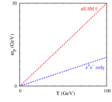
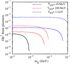
Figure 12: To compare contributions from $e^{+}e^{-}$ only with that of all fermions: (a) plasma frequency for the two cases (b) DM relic density produced by considering electrons only (dotted lines) and all SM fermions (dashed lines) as a function of DM mass, for different reheating temperatures. For $T_{RH}=1\,$GeV, the two lines can be seen to coincide.

Appendix B Lenard’s Formula for Inelastic Case

Lenard’s formula for our case is Lenard:1953zz :

$$\int\frac{d^{3}p_{\chi_{1}}}{(2\pi)^{3}\,(2E_{\chi_{1}})}\frac{d^{3}p_{\chi_{2}}}{(2\pi)^{3}\,(2E_{\chi_{2}})}(2\pi)^{4}\delta^{4}\left(k-p_{\chi_{1}}-p_{\chi_{2}}\right)p^{\mu}_{\chi_{1}}p^{\nu}_{\chi_{2}}=\frac{1}{96\pi}\left(A\,k^{2}g^{\mu\nu}+2B\,k^{\mu}k^{\nu}\right).$$ (66)

Multiplying both sides by $g^{\mu\nu}$ and contracting, we get

$$k^{2}(4A+2B) = 96\pi\left(p_{\chi_{1}}.p_{\chi_{2}}\right)\int\frac{d^{3}p_{\chi_{1}}}{(2\pi)^{3}\,(2E_{\chi_{1}})}\frac{d^{3}p_{\chi_{2}}}{(2\pi)^{3}\,(2E_{\chi_{2}})}(2\pi)^{4}\delta^{4}\left(k-p_{\chi_{1}}-p_{\chi_{2}}\right)$$ (67)

$$(4A+2B) = \frac{96\pi}{2}\left(1-\frac{m_{\chi_{1}}^{2}+m_{\chi_{2}}^{2}}{s}\right)$$ (68)

$$\quad\times\int\frac{d^{3}p_{\chi_{1}}}{(2\pi)^{3}\,(2E_{\chi_{1}})}\frac{d^{3}p_{\chi_{2}}}{(2\pi)^{3}\,(2E_{\chi_{2}})}(2\pi)^{4}\delta^{4}\left(k-p_{\chi_{1}}-p_{\chi_{2}}\right)$$

$$= 12\;C_{1}\left(1-\frac{m_{\chi_{1}}^{2}+m_{\chi_{2}}^{2}}{s}\right)$$ (69)

where $k^{2}=s$. Here, the integration on RHS has been carried out in the rest frame of plasmon:

$$\int\frac{d^{3}p_{\chi_{2}}}{(2\pi)^{3}(2E_{\chi_{2}})}\frac{d^{3}p_{\chi_{1}}}{(2\pi)^{3}(2E_{\chi_{1}})}(2\pi)^{4}\delta^{4}\left(k-p_{\chi_{1}}-p_{\chi_{2}}\right)=$$

$$\quad\quad\int\frac{d^{3}p_{\chi}^{*}}{(2\pi)^{2}\,4(E_{\chi_{2}}^{*}E_{\chi_{1}}^{*})}\times\,\delta^{0}\left(\omega^{*}-\sqrt{|p_{\chi}^{*}|^{2}+m_{\chi_{2}}^{2}}-\sqrt{|p_{\chi}^{*}|^{2}+m_{\chi_{1}}^{2}}\right)\qquad$$ (70)

where the $\vec{p}_{\chi_{1}}$ integral just sets $\vec{p}_{\chi_{1}}=\vec{p}_{\chi_{2}}$. Then we do the $\vec{p}_{\chi_{2}}$ integral in the rest frame of plasmon, defining all quantities in this frame with a ^∗ and redefining $p_{\chi_{2}}^{*}\equiv p_{\chi}^{*}$.

We simplify the delta function as

$$\delta^{0}\left(\omega^{*}-\sqrt{|p_{\chi}^{*}|^{2}+m_{\chi_{2}}^{2}}-\sqrt{|p_{\chi}^{*}|^{2}+m_{\chi_{1}}^{2}}\right)=\frac{E^{0}_{\chi_{1}}E^{0}_{\chi_{2}}}{|p_{\chi}^{*}|_{0}(E^{0}_{\chi_{1}}+E^{0}_{\chi_{2}})}\delta^{0}\left(|p_{\chi}^{*}|-|p_{\chi}^{*}|_{0}\right),$$ (71)

where,

$$|p_{\chi}^{*}|_{0} = \sqrt{\left(\frac{(\omega^{*})^{2}+m_{\chi_{2}}^{2}-m_{\chi_{1}}^{2}}{2\omega^{*}}\right)^{2}-m_{\chi_{2}}^{2}}=\sqrt{\frac{\lambda\left((\omega^{*})^{2},m_{\chi_{2}}^{2},m_{\chi_{1}}^{2}\right)}{4(\omega^{*})^{2}}},$$ (72)

$${\rm and,}\qquad E^{0}_{\chi_{i}} = \sqrt{m_{\chi_{i}}^{2}+|p_{\chi}^{*}|_{0}^{2}}.$$ (73)

Here, $\lambda$ is the Källén function defined as $\lambda(a,b,c)=a^{2}+b^{2}+c^{2}-2ab-2ac-2bc$. Plugging this into eq. (70) we get

$$\int\frac{d^{3}p_{\chi_{2}}}{(2\pi)^{3}\,(2E_{\chi_{2}})}\frac{d^{3}p_{\chi_{1}}}{(2\pi)^{3}\,(2E_{\chi_{1}})}(2\pi)^{4}\delta^{4}\left(k-p_{\chi_{1}}-p_{\chi_{2}}\right)=\frac{1}{4\pi}\frac{|p_{\chi}^{*}|_{0}}{E^{0}_{\chi_{1}}+E^{0}_{\chi_{2}}}=\frac{1}{4\pi}C_{1},$$ (74)

$$\,\text{where,}\,\,\,C_{1}=\frac{\sqrt{\left(\frac{s+m_{\chi_{2}}^{2}-m_{\chi_{1}}^{2}}{2\sqrt{s}}\right)^{2}-m_{\chi_{2}}^{2}}}{\frac{s+m_{\chi_{2}}^{2}-m_{\chi_{1}}^{2}}{2\sqrt{s}}+\sqrt{\left(\frac{s+m_{\chi_{2}}^{2}-m_{\chi_{1}}^{2}}{2\sqrt{s}}\right)^{2}-m_{\chi_{2}}^{2}+m_{\chi_{1}}^{2}}}$$ (75)

Here, we have used $s=k^{2}=\omega_{*}^{2}\text{ (in CM frame},\vec{k}_{*}=0\implies k_{*}^{2}=\omega_{*}^{2})$.
Subsequently, multiplying both sides of eq. (66) by $k^{\mu}k^{\nu}$ and contracting, we get

$$k^{4}(A+2B)=96\pi\;(k.p_{\chi_{1}})(k.p_{\chi_{2}})\int\frac{d^{3}p_{\chi_{1}}}{(2\pi)^{3}\,(2E_{\chi_{1}})}\frac{d^{3}p_{\chi_{2}}}{(2\pi)^{3}\,(2E_{\chi_{2}})}(2\pi)^{4}\delta^{4}\left(k-p_{\chi_{1}}-p_{\chi_{2}}\right).$$ (76)

Using $k=(p_{\chi_{1}}+p_{\chi_{2}})$,

$$(k-p_{\chi_{1}})^{2}=p_{\chi_{2}}^{2}\implies k^{2}+m_{\chi_{1}}^{2}-2\;k.p_{\chi_{1}}=m_{\chi_{2}}^{2}\implies k.p_{\chi_{1}}=\frac{k^{2}-m_{\chi_{2}}^{2}+m_{\chi_{1}}^{2}}{2},$$

$$(k-p_{\chi_{2}})^{2}=p_{\chi_{1}}^{2}\implies k^{2}+m_{\chi_{2}}^{2}-2\;k.p_{\chi_{2}}=m_{\chi_{1}}^{2}\implies k.p_{\chi_{2}}=\frac{k^{2}-m_{\chi_{1}}^{2}+m_{\chi_{2}}^{2}}{2},$$

and substituting from eq. (74), we get:

$$(A+2B)=6C_{1}\left(1+\frac{m_{\chi_{1}}^{2}-m_{\chi_{2}}^{2}}{s}\right)\left(1+\frac{m_{\chi_{2}}^{2}-m_{\chi_{1}}^{2}}{s}\right)$$ (77)

Putting together eqs. (69) and (77), we get

$$A=2C_{1}\left(1+\left(\frac{m_{\chi_{2}}^{2}-m_{\chi_{1}}^{2}}{s}\right)^{2}-2\left(\frac{m_{\chi_{1}}^{2}+m_{\chi_{2}}^{2}}{s}\right)\right)$$ (78)

$$B=2C_{1}\left(1+\left(\frac{m_{\chi_{2}}^{2}+m_{\chi_{1}}^{2}}{s}\right)-2\left(\frac{m_{\chi_{2}}^{2}-m_{\chi_{1}}^{2}}{s}\right)^{2}\right)$$ (79)

for the inelastic Lenard’s formula, eq.(66), with $C_{1}$ given in eq. (75)

Appendix C Fixed Target: NA64 Events

We review the discussion in ref. Chu:2018qrm and begin by noting that in full generality, a 4-body phase space has 12 degrees of freedom. In particular, though, there are redundancies from invariance in rotation around the beam line, and from imposition of energy-momentum conservation, leaving us with 7 independent degrees of freedom. With this knowledge, the 4-body phase space can be written as

$$\frac{d\Phi_{4}}{ds_{3\chi_{1}\chi_{2}}dq_{2}^{2}}=\frac{|J|}{16(2\pi)^{6}}\frac{ds_{\chi_{1}\chi_{2}}}{s_{\chi_{1}\chi_{2}}}dq_{1}^{2}\frac{\lambda^{1/2}\left(s_{\chi_{1}\chi_{2}},m_{\chi_{1}}^{2},m_{\chi_{2}}^{2}\right)}{\lambda^{1/2}\left(s_{3\chi_{1}\chi_{2}},m_{N}^{2},q_{2}^{2}\right)}du_{2_{q}}\Bigg{|}\frac{\partial\phi_{3}^{R3\chi_{1}\chi_{2}}}{\partial u_{2_{q}}}\Bigg{|}\frac{d\Omega_{\chi}^{R\chi_{1}\chi_{2}}}{4\pi},$$ (80)

where the kinematic quantities are,

$$s_{3\chi_{1}\chi_{2}} =(p_{3}+p_{\chi_{1}}+p_{\chi_{2}})^{2},$$

$$s_{\chi_{1}\chi_{2}} =q^{2}=(p_{\chi_{1}}+p_{\chi_{2}})^{2},$$

$$u_{2_{q}} =p_{2}.q$$

Here, $q_{2}=p_{2}-p_{4}$, $q_{1}=p_{1}-p_{3}$ and the remaining momenta are as shown in fig. 5. The azimuthal angle of $p_{3}$ in the frame where $\vec{p}_{3}+\vec{p}_{\chi_{1}}+\vec{p}_{\chi_{2}}=0$ is given by $\phi_{3}^{R3\chi_{1}\chi_{2}}$ and the solid angle between the DM particles is $\Omega_{\chi}^{R\chi_{1}\chi_{2}}$. The Källén function denoted by $\lambda$ is defined as

$$\lambda(a,b,c)=a^{2}+b^{2}+c^{2}-2ab-2ac-2bc.$$

The Jacobian of the transformation from $E_{4},{\rm cos}\theta_{4}$ to $s_{3\chi_{1}\chi_{2}},q_{2}^{2}$, required to connect between eq. (36) and eq. (80), is given by

$$\frac{\partial(E_{4},\textrm{cos}\,\theta_{4})}{\partial(s_{3\chi_{1}\chi_{2}},q_{2}^{2})}=\frac{|J|}{|\vec{p}_{4}|}\equiv\frac{\lambda^{-1/2}(s,m_{N}^{2},m_{e}^{2})}{2|\vec{p}_{4}|}$$ (81)

The double differential cross section for the production corresponding to fig. 5 is

$$\frac{d\sigma_{prod}}{dE_{4}d\textrm{cos}\,\theta_{4}}=\frac{|\vec{p}_{4}|}{4E_{2}m_{N}|\vec{v}_{2}|}\int\frac{d\Phi_{4}}{ds_{3\chi_{1}\chi_{2}}dq_{2}^{2}}\frac{1}{|J|}|\mathcal{M}|^{2},$$ (82)

where $E_{2}=E_{0}$ is the incoming electron (beam) energy with its velocity given as $|\vec{v}_{2}|=\sqrt{1-(m_{e}/E_{0})^{2}}$.

The squared amplitude for the process shown in fig. 5 is

$$|\mathcal{M}|^{2}=(4\pi\alpha)^{3}\frac{2}{q^{4}q_{1}^{4}}L^{\rho\sigma,\mu\nu}\chi_{\mu\nu}(q)W_{\rho\sigma}(-q_{1})\Bigg{|}_{s_{X}=m_{N}^{2}},$$ (83)

with $\chi_{\mu\nu}$ the DM emission piece of the amplitude,

$$\chi_{\mu\nu}=\textrm{Tr}\left[(\not{p}_{\chi_{1}}+m_{\chi_{1}})\Gamma_{\mu}(q)(\not{p}_{\chi_{2}}-m_{\chi_{2}})\bar{\Gamma}_{\nu}(q)\right].$$ (84)

Here, the interaction operators are given by $\Gamma^{\mu}(q)=-d_{\chi}\sigma^{\mu\nu}q_{\nu}\gamma^{5}$ for EDM and $\Gamma^{\mu}(q)=i\mu_{\chi}\sigma^{\mu\nu}q_{\nu}$ for MDM. The term corresponding to electron scattering, with averaging over initial and sum over final spins is

$$L^{\rho\sigma,\mu\nu} =\frac{L^{\rho\sigma,\mu\nu}_{a}}{[(p_{4}+q)^{2}-m_{e}^{2}]^{2}}+\frac{L^{\rho\sigma,\mu\nu}_{b}}{[(p_{2}-q)^{2}-m_{e}^{2}]^{2}}+\frac{2L^{\rho\sigma,\mu\nu}_{ab}}{[(p_{4}+q)^{2}-m_{e}^{2}][(p_{2}-q)^{2}-m_{e}^{2}]}$$ (85)

$$\textrm{with, \,}L^{\rho\sigma,\mu\nu}_{a} =\frac{1}{2}\textrm{Tr}\left[(\not{p}_{4}+m_{e})\gamma^{\mu}(\not{p}_{4}+\not{q}+m_{e})\gamma^{\rho}(\not{p}_{2}+m_{e})\gamma^{\sigma}(\not{p}_{4}+\not{q}+m_{e})\gamma^{\nu}\right]$$

$$L^{\rho\sigma,\mu\nu}_{b} =\frac{1}{2}\textrm{Tr}\left[(\not{p}_{2}+m_{e})\gamma^{\nu}(\not{p}_{2}-\not{q}+m_{e})\gamma^{\sigma}(\not{p}_{4}+m_{e})\gamma^{\rho}(\not{p}_{2}-\not{q}+m_{e})\gamma^{\mu}\right]$$

$$L^{\rho\sigma,\mu\nu}_{ab} =\frac{1}{2}\textrm{Tr}\left[(\not{p}_{4}+m_{e})\gamma^{\mu}(\not{p}_{4}+\not{q}+m_{e})\gamma^{\rho}(\not{p}_{2}+m_{e})\gamma^{\sigma}(\not{p}_{2}-\not{q}+m_{e})\gamma^{\nu}\right].$$

The hadronic tensor describing the response of the nuclear target is

$$W^{\rho\sigma}\simeq\left(p_{1}^{\rho}-\frac{p_{1}.q_{1}}{q_{1}^{2}}q_{1}^{\rho}\right)\left(p_{1}^{\sigma}-\frac{p_{1}.q_{1}}{q_{1}^{2}}q_{1}^{\sigma}\right)\frac{W(q_{1}^{2},s_{X})}{m_{N}^{2}}.$$ (86)

Assuming Pb to be a scalar target gives

$$W_{1}(q^{2}) =0,$$

$$W_{2}(q^{2}) =4m_{N}^{2}F_{E}^{2}(q_{1}^{2})\delta(s_{X}-m_{N}^{2})/2,$$

with, $F_{E}(t)=Z\frac{a^{2}(Z)t}{1+a^{2}(Z)t}\frac{1}{1+t/d(A)}$, $t=-q_{1}^{2}$, $a(Z)=111\frac{Z^{1/3}}{m_{e}}$ and $d(A)=0.164$ GeV${}^{2}A^{-2/3}$. The mass number and atomic number of the target nucleus are given by $A$ and $Z$, respectively. We have neglected the magnetic form factor for $Z>>1$.

The integration boundaries for eq. (82) are:

$$(m_{N}+m_{\chi_{1}}+m_{\chi_{2}})^{2}\leq s_{3\chi_{1}\chi_{2}}\leq(\sqrt{s}-m_{e})^{2},$$

$$(m_{\chi_{1}}+m_{\chi_{2}})^{2}\leq s_{\chi_{1}\chi_{2}}\leq(\sqrt{s_{3\chi_{1}\chi_{2}}}-m_{N})^{2},$$

$$[q_{1}^{2}]^{\pm} =2m_{N}^{2}-\frac{(s_{3\chi_{1}\chi_{2}}+m_{N}^{2}-q_{2}^{2})(s_{3\chi_{1}\chi_{2}}+m_{N}^{2}-s_{\chi_{1}\chi_{2}})}{2s_{3\chi_{1}\chi_{2}}}$$

$$\mp\frac{\lambda^{1/2}(s_{3\chi_{1}\chi_{2}},m_{N}^{2},q_{2}^{2})\lambda^{1/2}(s_{3\chi_{1}\chi_{2}},m_{N}^{2},s_{\chi_{1}\chi_{2}})}{2s_{3\chi_{1}\chi_{2}}},$$

$$[q_{2}^{2}]^{\pm} =2m_{e}^{2}-\frac{(s+m_{e}^{2}-m_{N}^{2})(s+m_{e}^{2}-s_{3\chi_{1}\chi_{2}})}{2s}\mp\frac{\lambda^{1/2}(s,m_{e}^{2},m_{N}^{2})\lambda^{1/2}(s,m_{e}^{2},s_{3\chi_{1}\chi_{2}})}{2s}.$$

And the angular variable $u_{2_{q}}$ is given by

$$u_{2_{q}}= \frac{(p_{1}.p_{2})G_{2}(p_{1},q_{2};q_{2},q)}{-\Delta_{2}(p_{1},q_{2})}-\frac{(q_{2}.p_{2})G_{2}(p_{1},q_{2};p_{1},q)}{-\Delta_{2}(p_{1},q_{2})}$$

$$+\frac{\sqrt{\Delta_{3}(p_{1},q_{2},p_{2})\Delta_{3}(p_{1},q_{2},q)}}{-\Delta_{2}(p_{1},q_{2})}\textrm{cos}\,\phi_{3}^{R3\chi_{1}\chi_{2}}$$

where $G_{n}$ is the Gram determinant of dimension n and $\Delta_{n}$ is the Cayley determinant (symmetric Gram determinant) Han:2005mu ; Byckling:1971vca .
And finally, since the NA64 experiment isn’t sensitive to the angular distribution of the outgoing DM particles, we can integrate over the solid angle between the DM particles, $\Omega_{\chi}^{R\chi_{1}\chi_{2}}$ in eq. (80).

Appendix D Derivation of the electron recoil rate formula for upscattered DM

We follow the discussion in Appendix A of Essig et al Essig:2015cda to re-derive the electron scattering rate for a general DM flux.

The integrated flux changes as follows in going from the Standard Halo Model DM distribution $\left(g_{\chi}(v)\right)$ to a generic incoming DM flux per unit energy $\left(d\Phi/dK_{\chi_{2}}\right)$

$$\int dv\,g_{\chi}(v)\frac{\rho_{\chi}}{m_{\chi}}v\rightarrow\int dK_{\chi_{2}}\frac{d\Phi}{dK_{\chi_{2}}}$$ (87)

Then, starting from eq. A12 of Essig:2015cda , we rewrite the cross section for a $\chi_{2}$ to excite an electron from level 1 to level 2 of an atom as

$$\sigma_{1\rightarrow 2}=\frac{\bar{\sigma}_{e}}{4\mu_{\chi_{2},e}^{2}v}\int\frac{d^{3}q}{4\pi}\delta\left(\Delta E_{1\rightarrow 2}+\frac{q^{2}}{2m_{\chi_{2}}}-q\,v\,{\rm cos}\theta_{qv}\right)|F_{DM}(q)|^{2}|f_{1\rightarrow 2}(q)|^{2}\bigg{|}_{v=\sqrt{2K_{\chi_{2}}/m_{\chi_{2}}}}.$$ (88)

The rate of excitation events, for a given transition and given target electrons, is found by multiplying eq. (88) by the incoming $\chi_{2}$ flux. Using eq. (87) we get this to be

$$R_{1\rightarrow 2} = \int dK_{\chi_{2}}\frac{d\Phi}{dK_{\chi_{2}}}\sigma_{1\rightarrow 2}\,$$ (90)

$$= \int dK_{\chi_{2}}\frac{d\Phi}{dK_{\chi_{2}}}\frac{\bar{\sigma}_{e}}{4\mu_{\chi_{2},e}^{2}}\sqrt{\frac{m_{\chi_{2}}}{2K_{\chi_{2}}}}\int\frac{d^{3}q}{4\pi}\delta\left(\Delta E_{1\rightarrow 2}+\frac{q^{2}}{2m_{\chi_{2}}}-q\sqrt{\frac{2K_{\chi_{2}}}{m_{\chi_{2}}}}{\rm cos}\theta_{qv}\right)$$

$$\qquad\times|F_{DM}(q)|^{2}|f_{1\rightarrow 2}(q)|^{2}.$$

The rates for ionization of electrons bound in isolated atoms can be calculated with the simplifying assumptions of a spherically symmetric atomic potential and filled shells. The ionized electron can be treated as being in one of a continuum of positive-energy bound states, approximated to free particle states at asymptotically large radii. The ionization rate for an atom is found by taking eq. (88), summing over occupied electron shells, and integrating over all possible final states. For ionization, with the final states being a continuum, the phase space is Essig:2015cda

$$\textrm{ionized electron phase space=}\sum_{l^{\prime}m^{\prime}}\int\frac{k^{\prime 2}dk^{\prime}}{(2\pi)^{3}}=\frac{1}{2}\sum_{l^{\prime}m^{\prime}}\int\frac{k^{\prime 3}d{\rm ln}\,E_{R}}{(2\pi)^{3}}.$$ (91)

Here, $l^{\prime},m^{\prime}$ are the angular quantum numbers of the ionized electron final state and $k^{\prime}$ is its momentum at asymptotically large distances from the nucleus, with energy $E_{R}=k^{\prime 2}/2m_{e}$. Plugging this in, the ionization rate is given as

$$R_{\rm ion} = \sum_{\textrm{occ. states}}\sum_{l^{\prime}m^{\prime}}\int dK_{\chi_{2}}\frac{k^{\prime 3}d{\rm ln}E_{R}}{2(2\pi)^{3}}\frac{d\Phi}{dK_{\chi_{2}}}\frac{\bar{\sigma}_{e}}{4\mu_{\chi_{2},e}^{2}}\sqrt{\frac{m_{\chi_{2}}}{2K_{\chi_{2}}}}$$ (93)

$$\qquad\times\int\frac{d^{3}q}{4\pi}\delta\left(\Delta E_{1\rightarrow 2}+\frac{q^{2}}{2m_{\chi_{2}}}-q\sqrt{\frac{2K_{\chi_{2}}}{m_{\chi_{2}}}}{\rm cos}\theta_{qK_{\chi_{2}}}\right)|F_{DM}(q)|^{2}|f_{i\rightarrow k^{\prime}l^{\prime}m^{\prime}}(q)|^{2}\,,$$

$$= \int dK_{\chi_{2}}d{\rm ln}E_{R}\frac{d\Phi}{dK_{\chi_{2}}}\frac{\bar{\sigma}_{e}}{16\mu_{\chi_{2},e}^{2}}\sqrt{\frac{m_{\chi_{2}}}{2K_{\chi_{2}}}}$$

$$\qquad\times\int\frac{d^{3}q}{4\pi}\delta\left(\Delta E_{1\rightarrow 2}+\frac{q^{2}}{2m_{\chi_{2}}}-q\sqrt{\frac{2K_{\chi_{2}}}{m_{\chi_{2}}}}{\rm cos}\theta_{qK_{\chi_{2}}}\right)|F_{DM}(q)|^{2}|f_{\rm ion}(k^{\prime},q)|^{2}\,,$$

with

$$|f_{\rm ion}(k^{\prime},q)|^{2}\equiv\frac{2k^{\prime 3}}{(2\pi)^{3}}\sum_{\textrm{occ. states}}\sum_{l^{\prime}m^{\prime}}|f_{i\rightarrow k^{\prime}l^{\prime}m^{\prime}}(q)|^{2}.$$ (94)

We can write the electron recoil energy spectrum per detector mass per unit time as

$$\frac{dR_{\rm ion}}{d\Delta E_{e}}=n_{T}\frac{\bar{\sigma}_{e}}{64\mu_{\chi_{2},e}^{2}}\sum_{n,l}\frac{1}{\Delta E_{e}-E_{nl}}\int dK_{\chi_{2}}\frac{d\Phi}{dK_{\chi_{2}}}\frac{m_{\chi_{2}}}{K_{\chi_{2}}}\int dq\,q|F_{DM}(q)|^{2}|f_{\rm ion}(k^{\prime},q)|^{2},$$ (95)

where the total energy transferred to the electron is $\Delta E_{e}=E_{R}+E_{nl}$ and $n_{T}$ is the number of targets per tonne. To explicitly show the order of integration, including the factor for depletion in numbers due to decay of $\chi_{2}$ in travelling from the Sun to the Earth, and the energy dependent detector efficiency ($\epsilon(\Delta E_{e})$), we get:

$$R_{\rm ion} = n_{T}\int d\Delta E_{e}\,\epsilon(\Delta E_{e})\sum_{n,l}\frac{1}{\Delta E_{e}-E_{nl}}\frac{\bar{\sigma}_{e}}{64\mu_{\chi_{2},e}^{2}}\int dK_{\chi_{2}}\Theta(\Delta E_{e}^{\rm max}(K_{\chi_{2}})-\Delta E_{e})\frac{d\Phi}{dK_{\chi_{2}}}\frac{m_{\chi_{2}}}{K_{\chi_{2}}}e^{-t(K_{\chi_{2}})\times\Gamma_{\chi_{2}}}$$ (96)

$$\qquad\qquad\times\int_{q^{-}(K_{\chi_{2}},\Delta E_{e},\delta,m_{\chi_{2}})}^{q^{+}(K_{\chi_{2}},\Delta E_{e},\delta,m_{\chi_{2}})}dq\,q|F_{DM}(q)|^{2}|f_{nl\rightarrow\Delta E_{e}-E_{nl}}(q)|^{2}.$$

Appendix E Effect of accounting for detector resolution in recoil spectra

We integrate over the theoretical differential event rate as given in eq. (23) to get the total number of events (shown by the color palette in fig. 7). For comparison with the experimental data, the theoretical spectra can be further smeared using a Gaussian distribution with energy-dependent width XENON:2020rca ; Lee:2020wmh

$$\frac{dR_{D}}{\Delta E_{e}}(\Delta E_{e})=\frac{R_{D}}{\sqrt{2\pi}\sigma(\Delta E_{e})}\textrm{exp}\left(-\frac{(\Delta E_{e}-\delta)^{2}}{2\sigma(\Delta E_{e})^{2}}\right),$$ (97)

where $\sigma(E)$ is the recoil energy dependent energy resolution of the detector. In figures 13 and 14, we show the smeared spectra finding that in each case the signal+background rates still shows an excess over the background rates. We use the detector resolution from XENON1T with $\sigma(E)=a.\sqrt{E}+b.E$ and $a=0.310\pm 0.004\sqrt{\textrm{keV}}$, $b=0.0037\pm 0.003$ XENON:2020rca .

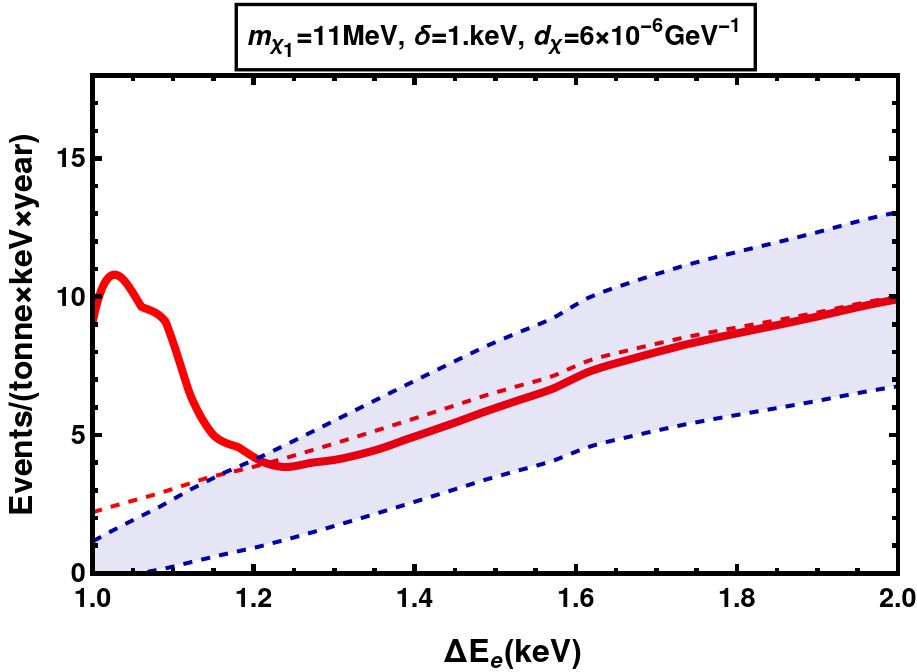
(a) $m_{\chi_{1}}=11$ MeV, $\delta=1\,$keV at XENONnT

(b) $m_{\chi_{1}}=11$ MeV, $\delta=1\,$keV at XeNONnT (proj.)

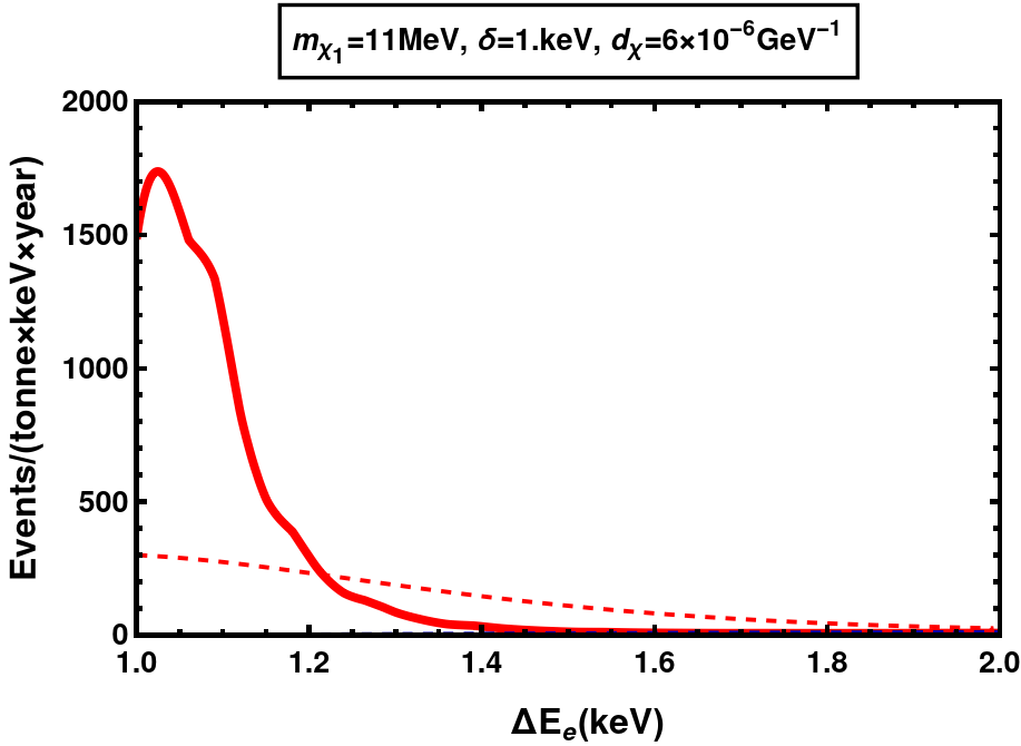
(c) $m_{\chi_{1}}=11$ MeV, $\delta=1\,$keV at DARWIN

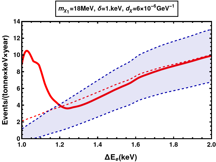
(d) $m_{\chi_{1}}=18$ MeV, $\delta=1\,$keV at XENONnT (proj.)

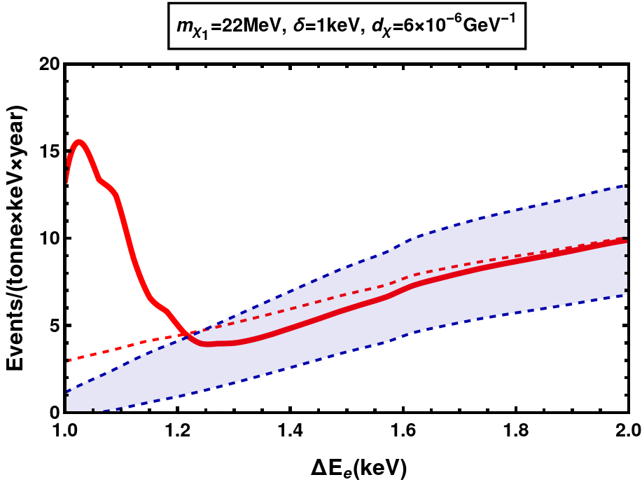
(e) $m_{\chi_{1}}=22$ MeV, $\delta=1\,$keV at DARWIN

Figure 13: Differential event rates for EDM DM. Shown in blue are the background rates with the band representing Poissonian $(\pm\sqrt{N})$ uncertainties. The dashed (solid) red lines show the signal+background rates with (without) smearing from detector resolution, using eq. (97) (eq. (23)).

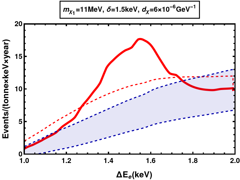
(a) $m_{\chi_{1}}=11{\rm MeV}$, $\delta=1.5{\rm keV}$ at XENONnT (proj.)

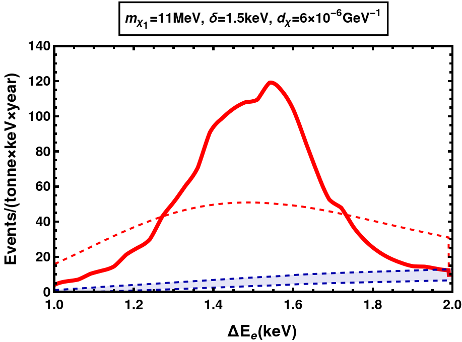
(b) $m_{\chi_{1}}=11$ MeV, $\delta=1.5\,$keV at DARWIN

Figure 14: Differential event rates for EDM DM. Shown in blue are the background rates with the band representing Poissonian $(\pm\sqrt{N})$ uncertainties. The dashed (solid) red lines show the signal+background rates with (without) smearing from detector resolution, using eq. (97) (eq. (23)).

References

- [1] Amin Aboubrahim, Michael Klasen, and Pran Nath. Xenon-1T excess as a possible signal of a sub-GeV hidden sector dark matter. JHEP, 02:229, 2021.
- [2] P. Achard et al. Single photon and multiphoton events with missing energy in collisions at LEP. Phys. Lett. B, 587:16–32, 2004.
- [3] Prateek Agrawal et al. Feebly-interacting particles: FIPs 2020 workshop report. Eur. Phys. J. C, 81(11):1015, 2021.
- [4] E. N. Alekseev, L. N. Alekseeva, I. V. Krivosheina, and V. I. Volchenko. Detection of the Neutrino Signal From SN1987A in the LMC Using the Inr Baksan Underground Scintillation Telescope. Phys. Lett. B, 205:209–214, 1988.
- [5] Haider Alhazmi, Doojin Kim, Kyoungchul Kong, Gopolang Mohlabeng, Jong-Chul Park, and Seodong Shin. Implications of the XENON1T Excess on the Dark Matter Interpretation. JHEP, 05:055, 2021.
- [6] Gonzalo Alonso-Álvarez, Fatih Ertas, Joerg Jaeckel, Felix Kahlhoefer, and Lennert J. Thormaehlen. Hidden Photon Dark Matter in the Light of XENON1T and Stellar Cooling. JCAP, 11:029, 2020.
- [7] Haipeng An, Maxim Pospelov, Josef Pradler, and Adam Ritz. Directly Detecting MeV-scale Dark Matter via Solar Reflection. Phys. Rev. Lett., 120(14):141801, 2018. [Erratum: Phys.Rev.Lett. 121, 259903 (2018)].
- [8] Haipeng An, Maxim Pospelov, Josef Pradler, and Adam Ritz. New limits on dark photons from solar emission and keV scale dark matter. Phys. Rev. D, 102:115022, 2020.
- [9] Haipeng An and Daneng Yang. Direct detection of freeze-in inelastic dark matter. Phys. Lett. B, 818:136408, 2021.
- [10] S. Andreas et al. Proposal for an Experiment to Search for Light Dark Matter at the SPS. 12 2013.
- [11] E. Aprile et al. Light Dark Matter Search with Ionization Signals in XENON1T. Phys. Rev. Lett., 123(25):251801, 2019.
- [12] E. Aprile et al. Search for Light Dark Matter Interactions Enhanced by the Migdal Effect or Bremsstrahlung in XENON1T. Phys. Rev. Lett., 123(24):241803, 2019.
- [13] E. Aprile et al. Excess electronic recoil events in XENON1T. Phys. Rev. D, 102(7):072004, 2020.
- [14] E. Aprile et al. Search for New Physics in Electronic Recoil Data from XENONnT. Phys. Rev. Lett., 129(16):161805, 2022.
- [15] Giorgio Arcadi, Andreas Bally, Florian Goertz, Karla Tame-Narvaez, Valentin Tenorth, and Stefan Vogl. EFT interpretation of XENON1T electron recoil excess: Neutrinos and dark matter. Phys. Rev. D, 103(2):023024, 2021.
- [16] Bernard Aubert et al. Search for Invisible Decays of a Light Scalar in Radiative Transitions A0. In 34th International Conference on High Energy Physics, 7 2008.
- [17] Seungwon Baek. Inelastic dark matter, small scale problems, and the XENON1T excess. JHEP, 10:135, 2021.
- [18] Seungwon Baek, Jongkuk Kim, and P. Ko. XENON1T excess in local DM models with light dark sector. Phys. Lett. B, 810:135848, 2020.
- [19] John N. Bahcall, M. H. Pinsonneault, and Sarbani Basu. Solar models: Current epoch and time dependences, neutrinos, and helioseismological properties. Astrophys. J., 555:990–1012, 2001.
- [20] D. Banerjee et al. Search for vector mediator of Dark Matter production in invisible decay mode. Phys. Rev. D, 97(7):072002, 2018.
- [21] D. Banerjee et al. Dark matter search in missing energy events with NA64. Phys. Rev. Lett., 123(12):121801, 2019.
- [22] Vernon Barger, Wai-Yee Keung, Danny Marfatia, and Po-Yan Tseng. Dipole Moment Dark Matter at the LHC. Phys. Lett. B, 717:219–223, 2012.
- [23] Masha Baryakhtar, Asher Berlin, Hongwan Liu, and Neal Weiner. Electromagnetic Signals of Inelastic Dark Matter Scattering. 6 2020.
- [24] Geneviève Bélanger, Fawzi Boudjema, Andreas Goudelis, Alexander Pukhov, and Bryan Zaldivar. micrOMEGAs5.0 : Freeze-in. Comput. Phys. Commun., 231:173–186, 2018.
- [25] Nicole F. Bell, James B. Dent, Bhaskar Dutta, Sumit Ghosh, Jason Kumar, and Jayden L. Newstead. Explaining the XENON1T excess with Luminous Dark Matter. Phys. Rev. Lett., 125(16):161803, 2020.
- [26] Nicole F. Bell, James B. Dent, Bhaskar Dutta, Sumit Ghosh, Jason Kumar, and Jayden L. Newstead. Low-mass inelastic dark matter direct detection via the Migdal effect. Phys. Rev. D, 104(7):076013, 2021.
- [27] R. Bernabei et al. On electromagnetic contributions in WIMP quests. Int. J. Mod. Phys. A, 22:3155–3168, 2007.
- [28] Nicolás Bernal, Matti Heikinheimo, Tommi Tenkanen, Kimmo Tuominen, and Ville Vaskonen. The Dawn of FIMP Dark Matter: A Review of Models and Constraints. Int. J. Mod. Phys. A, 32(27):1730023, 2017.
- [29] Biplob Bhattacherjee and Rhitaja Sengupta. XENON1T Excess: Some Possible Backgrounds. Phys. Lett. B, 817:136305, 2021.
- [30] R. M. Bionta et al. Observation of a Neutrino Burst in Coincidence with Supernova SN 1987a in the Large Magellanic Cloud. Phys. Rev. Lett., 58:1494, 1987.
- [31] James D. Bjorken, Rouven Essig, Philip Schuster, and Natalia Toro. New Fixed-Target Experiments to Search for Dark Gauge Forces. Phys. Rev. D, 80:075018, 2009.
- [32] Luc Blanchet and Alexandre Le Tiec. Dipolar Dark Matter and Dark Energy. Phys. Rev. D, 80:023524, 2009.
- [33] Itay M. Bloch, Andrea Caputo, Rouven Essig, Diego Redigolo, Mukul Sholapurkar, and Tomer Volansky. Exploring new physics with O(keV) electron recoils in direct detection experiments. JHEP, 01:178, 2021.
- [34] Celine Boehm, David G. Cerdeno, Malcolm Fairbairn, Pedro A. N. Machado, and Aaron C. Vincent. Light new physics in XENON1T. Phys. Rev. D, 102:115013, 2020.
- [35] Debasish Borah, Manoranjan Dutta, Satyabrata Mahapatra, and Narendra Sahu. Boosted Self-Interacting Dark Matter and XENON1T Excess. 7 2021.
- [36] Debasish Borah, Manoranjan Dutta, Satyabrata Mahapatra, and Narendra Sahu. Muon (g 2) and XENON1T excess with boosted dark matter in L L model. Phys. Lett. B, 820:136577, 2021.
- [37] Debasish Borah, Satyabrata Mahapatra, Dibyendu Nanda, and Narendra Sahu. Inelastic fermion dark matter origin of XENON1T excess with muon and light neutrino mass. Phys. Lett. B, 811:135933, 2020.
- [38] Eric Braaten and Daniel Segel. Neutrino energy loss from the plasma process at all temperatures and densities. Phys. Rev. D, 48:1478–1491, 1993.
- [39] Joseph Bramante and Ningqiang Song. Electric But Not Eclectic: Thermal Relic Dark Matter for the XENON1T Excess. Phys. Rev. Lett., 125(16):161805, 2020.
- [40] Jatan Buch, Manuel A. Buen-Abad, JiJi Fan, and John Shing Chau Leung. Galactic Origin of Relativistic Bosons and XENON1T Excess. JCAP, 10:051, 2020.
- [41] Ranny Budnik, Hyungjin Kim, Oleksii Matsedonskyi, Gilad Perez, and Yotam Soreq. Probing the relaxed relaxion and Higgs portal scenarios with XENON1T scintillation and ionization data. Phys. Rev. D, 104(1):015012, 2021.
- [42] Adam Burrows and James M. Lattimer. The birth of neutron stars. Astrophys. J., 307:178–196, 1986.
- [43] Dario Buttazzo, Paolo Panci, Daniele Teresi, and Robert Ziegler. Xenon1T excess from electron recoils of non-relativistic Dark Matter. Phys. Lett. B, 817:136310, 2021.
- [44] Eero Byckling and K. Kajantie. Particle Kinematics: (Chapters I-VI, X). University of Jyvaskyla, Jyvaskyla, Finland, 1971.
- [45] Qing-Hong Cao, Ran Ding, and Qian-Fei Xiang. Searching for sub-MeV boosted dark matter from xenon electron direct detection. Chin. Phys. C, 45(4):045002, 2021.
- [46] Mariana Carrillo González and Natalia Toro. Cosmology and Signals of Light Pseudo-Dirac Dark Matter. 8 2021.
- [47] Sabyasachi Chakraborty, Tae Hyun Jung, Vazha Loladze, Takemichi Okui, and Kohsaku Tobioka. Solar origin of the XENON1T excess without stellar cooling problems. Phys. Rev. D, 102(9):095029, 2020.
- [48] Jae Hyeok Chang, Rouven Essig, and Samuel D. McDermott. Revisiting Supernova 1987A Constraints on Dark Photons. JHEP, 01:107, 2017.
- [49] Jae Hyeok Chang, Rouven Essig, and Samuel D. McDermott. Supernova 1987A Constraints on Sub-GeV Dark Sectors, Millicharged Particles, the QCD Axion, and an Axion-like Particle. JHEP, 09:051, 2018.
- [50] Jae Hyeok Chang, Rouven Essig, and Annika Reinert. Light(ly)-coupled Dark Matter in the keV Range: Freeze-In and Constraints. JHEP, 03:141, 2021.
- [51] Wei Chao, Yu Gao, and Ming jie Jin. Pseudo-Dirac Dark Matter in XENON1T. 6 2020.
- [52] Shao-Long Chen and Zhaofeng Kang. On UltraViolet Freeze-in Dark Matter during Reheating. JCAP, 05:036, 2018.
- [53] Yifan Chen, Ming-Yang Cui, Jing Shu, Xiao Xue, Guan-Wen Yuan, and Qiang Yuan. Sun heated MeV-scale dark matter and the XENON1T electron recoil excess. JHEP, 04:282, 2021.
- [54] Cheng-Wei Chiang and Bo-Qiang Lu. Evidence of a simple dark sector from XENON1T excess. Phys. Rev. D, 102(12):123006, 2020.
- [55] So Chigusa, Motoi Endo, and Kazunori Kohri. Constraints on electron-scattering interpretation of XENON1T excess. JCAP, 10:035, 2020.
- [56] Gongjun Choi, Motoo Suzuki, and Tsutomu T. Yanagida. XENON1T Anomaly and its Implication for Decaying Warm Dark Matter. Phys. Lett. B, 811:135976, 2020.
- [57] Gongjun Choi, Tsutomu T. Yanagida, and Norimi Yokozaki. Feebly interacting gauge boson warm dark matter and XENON1T anomaly. Phys. Lett. B, 810:135836, 2020.
- [58] Soo-Min Choi, Hyun Min Lee, and Bin Zhu. Exothermic dark mesons in light of electron recoil excess at XENON1T. JHEP, 04:251, 2021.
- [59] Debajyoti Choudhury, Suvam Maharana, Divya Sachdeva, and Vandana Sahdev. Dark matter, muon anomalous magnetic moment, and the XENON1T excess. Phys. Rev. D, 103(1):015006, 2021.
- [60] Debtosh Chowdhury, Emilian Dudas, Maíra Dutra, and Yann Mambrini. Moduli Portal Dark Matter. Phys. Rev. D, 99(9):095028, 2019.
- [61] Xiaoyong Chu, Jui-Lin Kuo, and Josef Pradler. Dark sector-photon interactions in proton-beam experiments. Phys. Rev. D, 101(7):075035, 2020.
- [62] Xiaoyong Chu, Jui-Lin Kuo, Josef Pradler, and Lukas Semmelrock. Stellar probes of dark sector-photon interactions. Phys. Rev. D, 100(8):083002, 2019.
- [63] Xiaoyong Chu, Josef Pradler, and Lukas Semmelrock. Light dark states with electromagnetic form factors. Phys. Rev. D, 99(1):015040, 2019.
- [64] Jodi Cooley. Dark Matter Direct Detection of Classical WIMPs. In Les Houches summer school on Dark Matter, 10 2021.
- [65] Djuna Croon, Samuel D. McDermott, and Jeremy Sakstein. New physics and the black hole mass gap. Phys. Rev. D, 102(11):115024, 2020.
- [66] Djuna Croon, Samuel D. McDermott, and Jeremy Sakstein. Missing in axion: Where are XENON1T’s big black holes? Phys. Dark Univ., 32:100801, 2021.
- [67] Giancarlo D’Ambrosio, Shiuli Chatterjee, Ranjan Laha, and Sudhir K. Vempati. Freezing In with Lepton Flavored Fermions. SciPost Phys., 11:006, 2021.
- [68] Joe Davighi, Matthew McCullough, and Joseph Tooby-Smith. Undulating Dark Matter. JHEP, 11:120, 2020.
- [69] Hooman Davoudiasl, Peter B. Denton, and Julia Gehrlein. Attractive scenario for light dark matter direct detection. Phys. Rev. D, 102(9):091701, 2020.
- [70] Luigi Delle Rose, Gert Hütsi, Carlo Marzo, and Luca Marzola. Impact of loop-induced processes on the boosted dark matter interpretation of the XENON1T excess. JCAP, 02:031, 2021.
- [71] James B. Dent, Bhaskar Dutta, Jayden L. Newstead, and Adrian Thompson. Inverse Primakoff Scattering as a Probe of Solar Axions at Liquid Xenon Direct Detection Experiments. Phys. Rev. Lett., 125(13):131805, 2020.
- [72] William DeRocco, Peter W. Graham, and Surjeet Rajendran. Exploring the robustness of stellar cooling constraints on light particles. Phys. Rev. D, 102(7):075015, 2020.
- [73] Ujjal Kumar Dey, Tarak Nath Maity, and Tirtha Sankar Ray. Prospects of Migdal Effect in the Explanation of XENON1T Electron Recoil Excess. Phys. Lett. B, 811:135900, 2020.
- [74] Matthew J. Dolan, Felix Kahlhoefer, and Christopher McCabe. Directly detecting sub-GeV dark matter with electrons from nuclear scattering. Phys. Rev. Lett., 121(10):101801, 2018.
- [75] H. K. Dreiner, C. Hanhart, U. Langenfeld, and Daniel R. Phillips. Supernovae and light neutralinos: SN1987A bounds on supersymmetry revisited. Phys. Rev. D, 68:055004, 2003.
- [76] Jeff A. Dror, Gilly Elor, and Robert Mcgehee. Absorption of Fermionic Dark Matter by Nuclear Targets. JHEP, 02:134, 2020.
- [77] Jeff A. Dror, Gilly Elor, and Robert Mcgehee. Directly Detecting Signals from Absorption of Fermionic Dark Matter. Phys. Rev. Lett., 124(18):18, 2020.
- [78] Jeff A. Dror, Gilly Elor, Robert McGehee, and Tien-Tien Yu. Absorption of sub-MeV fermionic dark matter by electron targets. Phys. Rev. D, 103(3):035001, 2021.
- [79] Mingxuan Du, Jinhan Liang, Zuowei Liu, Van Que Tran, and Yilun Xue. On-shell mediator dark matter models and the Xenon1T excess. Chin. Phys. C, 45(1):013114, 2021.
- [80] Maira Dutra. Origins for dark matter particles : from the ”WIMP miracle” to the ”FIMP wonder”. PhD thesis, Orsay, LPT, 2019.
- [81] Koushik Dutta, Avirup Ghosh, Arpan Kar, and Biswarup Mukhopadhyaya. Decaying fermionic warm dark matter and XENON1T electronic recoil excess. Phys. Dark Univ., 33:100855, 2021.
- [82] Manoranjan Dutta, Satyabrata Mahapatra, Debasish Borah, and Narendra Sahu. Self-interacting Inelastic Dark Matter in the light of XENON1T excess. Phys. Rev. D, 103(9):095018, 2021.
- [83] Cora Dvorkin, Tongyan Lin, and Katelin Schutz. Making dark matter out of light: freeze-in from plasma effects. Phys. Rev. D, 99(11):115009, 2019.
- [84] Cora Dvorkin, Tongyan Lin, and Katelin Schutz. Cosmology of Sub-MeV Dark Matter Freeze-In. Phys. Rev. Lett., 127(11):111301, 2021.
- [85] Fatemeh Elahi, Christopher Kolda, and James Unwin. UltraViolet Freeze-in. JHEP, 03:048, 2015.
- [86] Yohei Ema, Filippo Sala, and Ryosuke Sato. Dark matter models for the 511 keV galactic line predict keV electron recoils on Earth. Eur. Phys. J. C, 81(2):129, 2021.
- [87] Timon Emken. Solar reflection of light dark matter with heavy mediators. Phys. Rev. D, 105(6):063020, 2022.
- [88] Timon Emken, Jonas Frerick, Saniya Heeba, and Felix Kahlhoefer. The ups and downs of inelastic dark matter: Electron recoils from terrestrial upscattering. 12 2021.
- [89] Rouven Essig, Marivi Fernandez-Serra, Jeremy Mardon, Adrian Soto, Tomer Volansky, and Tien-Tien Yu. Direct Detection of sub-GeV Dark Matter with Semiconductor Targets. JHEP, 05:046, 2016.
- [90] Rouven Essig, Jeremy Mardon, Michele Papucci, Tomer Volansky, and Yi-Ming Zhong. Constraining Light Dark Matter with Low-Energy Colliders. JHEP, 11:167, 2013.
- [91] Rouven Essig, Jeremy Mardon, and Tomer Volansky. Direct Detection of Sub-GeV Dark Matter. Phys. Rev. D, 85:076007, 2012.
- [92] Rouven Essig, Josef Pradler, Mukul Sholapurkar, and Tien-Tien Yu. Relation between the Migdal Effect and Dark Matter-Electron Scattering in Isolated Atoms and Semiconductors. Phys. Rev. Lett., 124(2):021801, 2020.
- [93] Marco Fabbrichesi, Emidio Gabrielli, and Gaia Lanfranchi. The Dark Photon. 5 2020.
- [94] Yasaman Farzan and M. Rajaee. Pico-charged particles explaining 511 keV line and XENON1T signal. Phys. Rev. D, 102(10):103532, 2020.
- [95] Anastasiia Filimonova, Sam Junius, Laura Lopez Honorez, and Susanne Westhoff. Inelastic Dirac Dark Matter. 1 2022.
- [96] Tobias Fischer, Sovan Chakraborty, Maurizio Giannotti, Alessandro Mirizzi, Alexandre Payez, and Andreas Ringwald. Probing axions with the neutrino signal from the next galactic supernova. Phys. Rev. D, 94(8):085012, 2016.
- [97] Bartosz Fornal, Pearl Sandick, Jing Shu, Meng Su, and Yue Zhao. Boosted Dark Matter Interpretation of the XENON1T Excess. Phys. Rev. Lett., 125(16):161804, 2020.
- [98] Jean-Francois Fortin and Tim M. P. Tait. Collider Constraints on Dipole-Interacting Dark Matter. Phys. Rev. D, 85:063506, 2012.
- [99] Christina Gao, Jia Liu, Lian-Tao Wang, Xiao-Ping Wang, Wei Xue, and Yi-Ming Zhong. Reexamining the Solar Axion Explanation for the XENON1T Excess. Phys. Rev. Lett., 125(13):131806, 2020.
- [100] Gian Francesco Giudice, Edward W. Kolb, and Antonio Riotto. Largest temperature of the radiation era and its cosmological implications. Phys. Rev. D, 64:023508, 2001.
- [101] S. N. Gninenko. Search for MeV dark photons in a light-shining-through-walls experiment at CERN. Phys. Rev. D, 89(7):075008, 2014.
- [102] Paolo Gondolo and Graciela Gelmini. Cosmic abundances of stable particles: Improved analysis. Nucl. Phys. B, 360:145–179, 1991.
- [103] Matt Graham, Christopher Hearty, and Mike Williams. Searches for Dark Photons at Accelerators. Ann. Rev. Nucl. Part. Sci., 71:37–58, 2021.
- [104] Anne M. Green. Dark Matter in Astrophysics/Cosmology. In Les Houches summer school on Dark Matter, 9 2021.
- [105] Gang Guo, Yue-Lin Sming Tsai, Meng-Ru Wu, and Qiang Yuan. Elastic and Inelastic Scattering of Cosmic-Rays on Sub-GeV Dark Matter. Phys. Rev. D, 102(10):103004, 2020.
- [106] Lawrence J. Hall, Karsten Jedamzik, John March-Russell, and Stephen M. West. Freeze-In Production of FIMP Dark Matter. JHEP, 03:080, 2010.
- [107] Thomas Hambye, Michel H. G. Tytgat, Jérôme Vandecasteele, and Laurent Vanderheyden. Dark matter direct detection is testing freeze-in. Phys. Rev. D, 98(7):075017, 2018.
- [108] Thomas Hambye, Michel H. G. Tytgat, Jérôme Vandecasteele, and Laurent Vanderheyden. Dark matter from dark photons: a taxonomy of dark matter production. Phys. Rev. D, 100(9):095018, 2019.
- [109] Tao Han. Collider phenomenology: Basic knowledge and techniques. In Theoretical Advanced Study Institute in Elementary Particle Physics: Physics in D 4, 8 2005.
- [110] Steen Hannestad. What is the lowest possible reheating temperature? Phys. Rev. D, 70:043506, 2004.
- [111] Keisuke Harigaya, Yuichiro Nakai, and Motoo Suzuki. Inelastic Dark Matter Electron Scattering and the XENON1T Excess. Phys. Lett. B, 809:135729, 2020.
- [112] Hong-Jian He, Yu-Chen Wang, and Jiaming Zheng. EFT Approach of Inelastic Dark Matter for Xenon Electron Recoil Detection. JCAP, 01:042, 2021.
- [113] Hong-Jian He, Yu-Chen Wang, and Jiaming Zheng. GeV-scale inelastic dark matter with dark photon mediator via direct detection and cosmological and laboratory constraints. Phys. Rev. D, 104(11):115033, 2021.
- [114] Gonzalo Herrera, Alejandro Ibarra, and Satoshi Shirai. Enhanced prospects for direct detection of inelastic dark matter from a non-galactic diffuse component. 1 2023.
- [115] K. Hirata et al. Observation of a Neutrino Burst from the Supernova SN 1987a. Phys. Rev. Lett., 58:1490–1493, 1987.
- [116] Masahiro Ibe, Wakutaka Nakano, Yutaro Shoji, and Kazumine Suzuki. Migdal Effect in Dark Matter Direct Detection Experiments. JHEP, 03:194, 2018.
- [117] Yongsoo Jho, Jong-Chul Park, Seong Chan Park, and Po-Yan Tseng. Leptonic New Force and Cosmic-ray Boosted Dark Matter for the XENON1T Excess. Phys. Lett. B, 811:135863, 2020.
- [118] Lian-Bao Jia and Tong Li. Interpretation of XENON1T excess with MeV boosted dark matter. 12 2020.
- [119] Kristjan Kannike, Martti Raidal, Hardi Veermäe, Alessandro Strumia, and Daniele Teresi. Dark Matter and the XENON1T electron recoil excess. Phys. Rev. D, 102(9):095002, 2020.
- [120] Wai-Yee Keung, Danny Marfatia, and Po-Yan Tseng. Stellar cooling, inelastic dark matter, and XENON. JHEAp, 30:9–15, 2021.
- [121] Sarif Khan. Explaining Xenon-1T signal with FIMP dark matter and neutrino mass in a extension. Eur. Phys. J. C, 81(7):598, 2021.
- [122] P. Ko and Yong Tang. Semi-annihilating dark matter for XENON1T excess. Phys. Lett. B, 815:136181, 2021.
- [123] N. V. Krasnikov. The Search for Light Dark Matter at NA64 Experiment. Phys. Part. Nucl., 51(4):697–702, 2020.
- [124] Robert Lasenby and Ken Van Tilburg. Dark photons in the solar basin. Phys. Rev. D, 104(2):023020, 2021.
- [125] Hyun Min Lee. Exothermic dark matter for XENON1T excess. JHEP, 01:019, 2021.
- [126] A. Lenard. Inner Bremsstrahlung in mu-Meson Decay. Phys. Rev., 90:968–973, 1953.
- [127] Manfred Lindner, Yann Mambrini, Téssio B. de Melo, and Farinaldo S. Queiroz. XENON1T anomaly: A light Z’ from a Two Higgs Doublet Model. Phys. Lett. B, 811:135972, 2020.
- [128] H. N. Long, D. V. Soa, V. H. Binh, and A. E. Cárcamo Hernández. Linking axion-like dark matter, the XENON1T excess, inflation and the tiny active neutrino masses. 7 2020.
- [129] Gabriel Magill, Ryan Plestid, Maxim Pospelov, and Yu-Dai Tsai. Dipole Portal to Heavy Neutral Leptons. Phys. Rev. D, 98(11):115015, 2018.
- [130] Eduard Masso, Subhendra Mohanty, and Soumya Rao. Dipolar Dark Matter. Phys. Rev. D, 80:036009, 2009.
- [131] John McDonald. Thermally generated gauge singlet scalars as selfinteracting dark matter. Phys. Rev. Lett., 88:091304, 2002.
- [132] David McKeen, Maxim Pospelov, and Nirmal Raj. Hydrogen Portal to Exotic Radioactivity. Phys. Rev. Lett., 125(23):231803, 2020.
- [133] AB Migdal. Ionization of atoms accompanying -and -decay. J. Phys. USSR, 4:449, 1941.
- [134] G. Montagna, O. Nicrosini, F. Piccinini, and L. Trentadue. Invisible events with radiative photons at LEP. Nucl. Phys. B, 452:161–172, 1995.
- [135] Kazunori Nakayama and Yong Tang. Gravitational Production of Hidden Photon Dark Matter in Light of the XENON1T Excess. Phys. Lett. B, 811:135977, 2020.
- [136] Nobuchika Okada, Satomi Okada, Digesh Raut, and Qaisar Shafi. Dark matter and XENON1T excess from extended standard model. Phys. Lett. B, 810:135785, 2020.
- [137] Sudhanwa Patra and Soumya Rao. A Simple Model for Magnetic Inelastic Dark Matter (MiDM). 12 2011.
- [138] Gil Paz, Alexey A. Petrov, Michele Tammaro, and Jure Zupan. Shining dark matter in Xenon1T. Phys. Rev. D, 103(5):L051703, 2021.
- [139] A. A. Prinz et al. Search for millicharged particles at SLAC. Phys. Rev. Lett., 81:1175–1178, 1998.
- [140] G. G. Raffelt. Stars as laboratories for fundamental physics: The astrophysics of neutrinos, axions, and other weakly interacting particles. 5 1996.
- [141] Alan E. Robinson. XENON1T observes tritium. 6 2020.
- [142] Tracy R. Slatyer. Les Houches Lectures on Indirect Detection of Dark Matter. In Les Houches summer school on Dark Matter, 9 2021.
- [143] Juri Smirnov and John F. Beacom. New Freezeout Mechanism for Strongly Interacting Dark Matter. Phys. Rev. Lett., 125(13):131301, 2020.
- [144] Liangliang Su, Wenyu Wang, Lei Wu, Jin Min Yang, and Bin Zhu. Atmospheric Dark Matter and Xenon1T Excess. Phys. Rev. D, 102(11):115028, 2020.
- [145] M. Szydagis, C. Levy, G. M. Blockinger, A. Kamaha, N. Parveen, and G. R. C. Rischbieter. Investigating the XENON1T low-energy electronic recoil excess using NEST. Phys. Rev. D, 103(1):012002, 2021.
- [146] Fuminobu Takahashi, Masaki Yamada, and Wen Yin. XENON1T Excess from Anomaly-Free Axionlike Dark Matter and Its Implications for Stellar Cooling Anomaly. Phys. Rev. Lett., 125(16):161801, 2020.
- [147] Yung-Su Tsai. Pair Production and Bremsstrahlung of Charged Leptons. Rev. Mod. Phys., 46:815, 1974. [Erratum: Rev.Mod.Phys. 49, 421–423 (1977)].
- [148] Neal Weiner and Itay Yavin. How Dark Are Majorana WIMPs? Signals from MiDM and Rayleigh Dark Matter. Phys. Rev. D, 86:075021, 2012.
- [149] Shuai Xu and Sibo Zheng. Resolving XENON Excess With Decaying Cold Dark Matter. Eur. Phys. J. C, 81(5):446, 2021.
- [150] Xiaopeng Zhou et al. A Search for Solar Axions and Anomalous Neutrino Magnetic Moment with the Complete PandaX-II Data. Chin. Phys. Lett., 38(1):011301, 2021. [Erratum: Chin.Phys.Lett. 38, 109902 (2021)].
- [151] Lei Zu, R. Foot, Yi-Zhong Fan, and Lei Feng. Plasma dark matter and electronic recoil events in XENON1T. JCAP, 01:070, 2021.
- [152] Lei Zu, Guan-Wen Yuan, Lei Feng, and Yi-Zhong Fan. Mirror Dark Matter and Electronic Recoil Events in XENON1T. Nucl. Phys. B, 965:115369, 2021.