Universal Thermodynamic Uncertainty Relation in Non-Equilibrium Dynamics
Abstract
We derive a universal thermodynamic uncertainty relation (TUR) that applies to an arbitrary observable in a general Markovian system. The generality of our result allows us to make two findings: (1) for an arbitrary out-of-equilibrium system, both the entropy production and the degree of non-stationarity are required to tightly bound the strength of a thermodynamic current; (2) by removing the antisymmetric constraint on observables, the TUR in physics and a fundamental inequality in theoretical finance can be unified in a single framework.
Introduction. Nature is rife with nonequilibrium phenomena such as expansion of the universe [1, 2, 3], relaxation dynamics of condensed matter systems [4, 5], interactions in ecological systems [6] and biological processes in living creatures [7, 8]. Nonequilibrium phenomena are not exclusive to natural sciences. The financial market is also a far-from-equilibrium system, with its complex dynamics arising from interactions among a large number of investors in the market [9, 10, 11]. The learning dynamics of deep neural networks is also regarded as an important nonequilibrium phenomenon [12, 13, 14, 15]. With such a wide range of applications, one naturally wonders what common features, if any, could be shared by all of these heterogeneous systems. Only after knowing what is shared across all nonequilibrium phenomena can we understand what is unique to each individual field and hope to unify nonequilibrium phenomena in different fields of natural and social sciences. This work studies the common features shared among various nonequilibrium problems and establishes a universal thermodynamic uncertainty relation applicable to general nonequilibrium dynamics.
To be concrete, we consider a trajectory of stochastic events across steps: , whose distribution is given by , and let be its time-reversed trajectory under the time-reversed protocol, whose distribution is denoted as . Each can be a set of real numbers if the relevant dynamics occurs in a continuous space or a set of discrete values if the space is discrete 111Also, to be concrete, we have specified to be a series of events in discrete time; we note that one can replace by a continuous-time trajectory and the sums by path integrals to show that in continuous time, our results remain unchanged.. We denote the average with respect to as , and that with respect to as . By the Markovian property, the trajectory probability factorizes into a product of the initial distribution and the transition probabilities
where the transition probabilities are explicitly labeled with to stress that the dynamics can be time-dependent.
It has recently been shown [17, 18, 19, 20, 21, 22, 23] that the average and variance of any thermodynamic quantity are related to the entropy production through the thermodynamic uncertainty relation (TUR):
| (1) |
where is a functional of entropy production , and is an antisymmetric current, which is odd under time reversal: . A physical interpretation of (1) is that the relative accuracy of a measurement is bounded from above by the entropy production [24]. A crucial observation here is that a more accurate measurement can be performed only at the cost of higher entropy production.
However, the original TUR only holds in a linear-response regime and is applicable to thermodynamic currents. Various attempts at generalizing the TUR have been made [25, 26, 27, 20, 28, 18, 29, 30, 31, 32, 33, 34]. Notably, Ref. [20] derives a TUR from the fluctuation theorem and the derived TUR is applicable to observables that are not limited to currents; however, it can only be applied to systems with strong constraints on the initial and final states of the system. Reference [18] generalizes the TUR to an arbitrary nonequilibrium initial state, where the bound only applies to the boundary value of the current. One of the most general forms of existing TUR proposed in Ref. [35] is applicable to an arbitrary reversible system and an arbitrary observable. However, this relation is still limited in the scope of applicability because it cannot be extended to the situations where the absolute irreversibility is involved 222The right-hand side of the proposal of [35] contains the term explicitly, which may diverge when the system is not fully reversible. The relation in [35] thus becomes a trivial relation: , where is a function of the relevant observable , whereas our result always remain meaningful. For detailed works about absolute irreversibility, see, for example, Ref. [58, 29, 38, 59]..
In this Letter, we overcome the limitations of the previous generalizations of the TUR and derive a universal TUR that is applicable to an arbitrary system with or without absolute irreversibility and to an arbitrary observable. Also, our result only involves the quantities that appeared in the original TUR. We prove the following universal inequality for an arbitrary observable 333See Appendix A for the proof.:
| (2) |
where is the log-probability ratio between the probability of the primary dynamics and a reference dynamics , and is the conditional expectation value of under , conditioned on . The freedom of choice of the reference dynamics is a generic feature of fluctuation theorems [38, 39]. The choice with physical relevance is , which makes the left-hand side of the inequality dependent on the entropy production: [38, 40]. The term on the left-hand side represents the degree of reversibility in the system, which is equal to (0) when it is fully reversible (irreversible) [38].
General Properties of the Universal TUR. If the reference dynamics is the time-reversed one of the forward dynamics, i.e., , then our TUR (2) leads to the following nontrivial relation between the current , its variance , the degree of absolute irreversibility , and the total entropy production :
| (3) |
This TUR is universal in that it applies to arbitrary initial and final states, allows for arbitrary time-dependent protocols, can be applied to arbitrary observables, makes no assumption about the transition probabilities, and is applicable to both continuous-time and discrete-time dynamics. The generality of the derived TUR is a consequence of the generality of the master fluctuation theorem, which finds its mathematical foundations in the general change-of-measure theorem in the measure theory [38]. A key feature of the this bound is that it involves an exponentiated entropy production, which may be dominated by rare trajectories [41]. However, we note that this is not a weakness of the proposed theory, but a reflection of the underlying physics that rare trajectories can have significant influence on the expected strength and fluctuation of physical quantities. This argument is further substantiated by the fact that no matter how strongly the term is dominated by the rare trajectories, there is always some observable that makes the bound satisfied.
The choice of suitable for the system and observable is crucial. For example, the entropy term is minimized when the reference dynamics is as close to the original one as possible; the current term is maximized when is chosen to make have a sign opposite to that of . We will see later that appropriate choices of lead to meaningful results for physics and theoretical finance. Also, the result in (2) achieves two types of optimality. Firstly, for every system, there exists an observable such that the bound is saturated. Secondly, for every observable , there exists and such that the bound is saturated 444See Appendix B for the proof.. These optimalities imply that having a different form of TUR leads to either a looser bound for some systems or making the bound inapplicable to some observables. For example, the standard TUR has a linear entropic term [27] in place of in our bound with . However, it is not hard to see that the standard TUR bound is trivial for any irreversible process: when the support of is a proper subset of that of , , so the left-hand side of the standard TUR (1) diverges, and we obtain the trivial result . Some bounds are more similar to ours and involve an exponential term, but with the plus sign in the exponent [25, 20]: ; this type of formula also cannot appear in the most general TUR because also diverges when . Among the three choices of the entropic term (, , ), only the form can remain finite.
Inequality (2) takes a simpler form for antisymmetric currents. Let the quantity be an antisymmetric current, the protocol be time-independent and the initial and final distributions are stationary, our TUR reduces to: 555See Appendix D. Expanding this relation to first order in , it recovers the original TUR in Ref. [17], which holds in the linear-response regime. Also, as in Ref. [30], we can also generalize the main result in (2) to a vector-valued observable as detailed in Appendix C, which is the most general TUR we derive. Lastly, we note that the proposed relation also takes a meaningful form in the equilibrium limit where approaches zero. We study this in Appendix F.
Application I – Interplay between the degree of non-stationarity and entropy production. When the transition probabilities are time-independent and , our result offers a crucial insight into the achievable measurement accuracy of a thermodynamic current that is antisymmetric against time reversal. Let and denote the initial and final distributions of the process . We choose to be the distribution resultant from the time-reversed dynamics, with as the initial distribution: . Then, (2) becomes
| (4) |
where 666We clarify that is not equal to the system-wise entropy change. Following Ref [60], the trajectory-wise system entropy change is , whereas the term in our bound is . The two are different in general., is the Kullback-Leibler divergence between the initial and final distributions. We see that measures the trajectory-wise distance between the initial distribution and the final (possibly non-stationary) distribution. The right-hand side of (4) is the relative accuracy. Noting that is zero when the system is stationary, it characterizes the “degree of non-stationarity.” Thus the interplay between the degree of non-stationarity and entropy production plays a key role in providing the accuracy of a thermodynamic current in the most general Markovian relaxation dynamics, whose initial and final distributions can be out-of-equilibrium. Specifically, we find that the maximum achievable accuracy decreases with an increasing deviation between the initial and final distributions. Physically, this strong dependence on the initial condition can be understood as follows: when measuring a local parameter close to a site , it is the most efficient for us to initialize the state of the system in the neighborhood of . If we choose the initial state according to the Boltzmann distribution, many states away from are involved, resulting in a reduced measurement efficiency.
The conventional TUR dictates that the bound on the measurement accuracy of antisymmetric currents increases as we increase the entropy production [40, 24]. On the contrary, our result implies that the measurement accuracy can decrease with an increasing entropy production when the system is out-of-equilibrium and when dominates the entropy production. Lastly, when the system is close to stationarity, becomes negligible, and one can show that the bound approximately reduces to , which, in agreement with the standard TUR, suggests that the limit of measurement accuracy should increase with the entropy production.
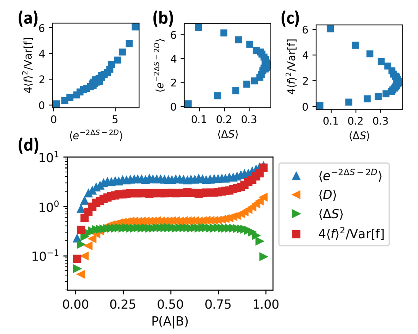
As an example, we numerically simulate an out-of-equilibrium two-state system. The two states are labeled as and . We let the initial state be and . The transition probability is set to be symmetric: . We study the bound at different , varying from zero to one. The observable we consider is the net number of transitions from state to state : , which is by definition an antisymmetric observable. Figure 1 shows the relevant quantities of this simulation. We see that the proposed relation (4) places a bound of the measurement accuracy of the far-from-equilibrium system across all transition probabilities, whereas the standard TUR is almost everywhere inapplicable. A detailed comparison is given in Appendix E, where we show that the bound in inequality (4) can be considerably tighter than other TURs.
Application II – A Fundamental Bound in Theoretical Finance. This example shows that it is, in fact, important to freely choose if we want to make the TUR relevant to general nonequilibrium dynamics in fields other than physics. The financial market is a major non-physical nonequilibrium system that impacts our daily life [45, 46]. Consider the price trajectory of a product (e.g., a stock) that changes from time to time , denoted as , where each unit of time corresponds to a day. The price return is defined as . Here, we assume that the price dynamics follows a discrete-time Markovian dynamics in continuous space. While this assumption may not hold in general, it holds for the standard minimal models in finance such as the Black-Scholes model [47] and the Heston model [48]. A key quantity is the volatility of the price return .
With , our TUR in (2) gives
| (5) |
which explicitly shows that the thermodynamic entropy production gives a bound on price volatility, which can be useful for problems such as option pricing. This may open a venue for studying quantitative finance in terms of stochastic thermodynamics. Moreover, since the price return is not a time-antisymmetric observable, the standard TUR cannot apply.
We now show that a fundamental inequality in theoretical finance can be derived as a special case of the general TUR in (2). By investing a fraction of one’s capital, , in the product at different times, one can make profit, which is measured with the wealth return rate : , where is the risk-free interest rate. In theoretical finance (capital asset pricing model), a fundamental quantity is the Sharpe ratio, defined as
| (6) |
where . Again, the observable is not antisymmetric, and therefore the standard TURs do not apply. The Sharpe ratio is widely accepted as a fundamental quantity in theoretical finance [49, 50] and used in practice as a metric of successful investment. Theoretically, it is known that optimal portfolios should all have the same maximized Sharpe ratio [49], and it is an important problem to find an upper bound on the Sharpe ratio.
For this problem, the relevant reference dynamics is no longer because in general. We need to choose to be the dynamics such that the wealth grows at the risk-free rate on average. This dynamics can be achieved if the stock price grows deterministically as , or if we create and transact a financial derivative according to the Black-Scholes formula. With , our TUR yields , or, equivalently,
| (7) |
for any trading strategy. The existence of such a is guaranteed by the fundamental theorem of finance (no-arbitrage theorem), and inequality (7) applies to any price dynamics that obeys the fundamental theorem of finance. In fact, this bound has the same form as the celebrated Hansen-Jagannathan (HJ) bound in theoretical finance [51, 52, 53]. The HJ bound is a fundamental relation in theoretical finance because it applies to all models of the market, and there have been many applications of it besides upper bounding the Sharpe ratio [54, 55, 56, 57]. While the original HJ bound can only be applied to the case in which is a martingale distribution, our result applies to an arbitrary distribution such that . The bound (5) is a new relation we discovered. One important utility of the proposed relation for finance is that it allows one to check the validity and correctness of existing theories of finance (this is also what the related Hansen–Jagannathan bound can be useful for). For example, existing stock price data allows one to estimate the return and its volatility , and the minimal models allow one to calculate the time-reversed return , and the entropic term , and this can be plugged into the proposed TUR relation, the violation of which can then be used to reject the economic theory under consideration. Our result thus offers a novel method to test the validity of economic theories with physics-relevant quantities (such as the entropy production rate), which presents yet another remarkable usage of physics principles in other fields.
This application shows that the HJ bound in finance is comparable to the thermodynamic uncertainty relations in physics, and the crucial difference between the two bounds arises from the choice of the reference probability . The choice of fundamental importance in physics is the time-reversed dynamics , while the fundamental choice in finance is the martingale measure, under which one obtains the risk-free return. Therefore, our derived TUR unifies the fundamental bounds in physics and finance.
Conclusion and discussion. We have derived a universal form of TUR for an arbitrary Markovian dynamics in discrete space-time, which includes the continuous space-time dynamics as a special limit. Our bound is shown to achieve two kinds of optimalities, but it is unlikely to be the optimal bound if we restrict the problem to systems of special types or observables with specific symmetries. Investigating how such constraints on observables may help improve the bound is an important future work. One crucial quantity identified in this work is the degree of non-stationarity , and it should be important to understand it better in the future. Our result also links the fundamentals in theoretical finance and physics, and further exploring this connection may lead to exciting cross-fertilization of both fields.
Acknowledgements.
This work was supported by a KAKENHI Grant No. JP18H01145 from the Japan Society for the Promotion of Science. Ziyin thanks Tonghua Yu and Junxia Wang for many thoughtful promenades they shared during the writing of this paper.References
- Kawasaki et al. [1999] M. Kawasaki, K. Kohri, and N. Sugiyama, Cosmological constraints on late-time entropy production, Physical Review Letters 82, 4168–4171 (1999).
- Berges [2015] J. Berges, Nonequilibrium quantum fields: From cold atoms to cosmology (2015), arXiv:1503.02907 [hep-ph] .
- Berges et al. [2004] J. Berges, S. Borsányi, and C. Wetterich, Prethermalization, Physical review letters 93, 142002 (2004).
- Polkovnikov et al. [2011] A. Polkovnikov, K. Sengupta, A. Silva, and M. Vengalattore, Colloquium: Nonequilibrium dynamics of closed interacting quantum systems, Reviews of Modern Physics 83, 863 (2011).
- Kamenev [2011] A. Kamenev, Field theory of non-equilibrium systems (Cambridge University Press, 2011).
- Rohde [2006] K. Rohde, Nonequilibrium ecology (Cambridge University Press, 2006).
- Fang and Wang [2020] X. Fang and J. Wang, Nonequilibrium thermodynamics in cell biology: Extending equilibrium formalism to cover living systems, Annual review of biophysics 49, 227 (2020).
- Wang [2015] J. Wang, Landscape and flux theory of non-equilibrium dynamical systems with application to biology, Advances in Physics 64, 1 (2015).
- Lux [2009] T. Lux, Applications of statistical physics in finance and economics, in Handbook of research on complexity (Edward Elgar Publishing, 2009).
- Samanidou et al. [2007] E. Samanidou, E. Zschischang, D. Stauffer, and T. Lux, Agent-based models of financial markets, Reports on Progress in Physics 70, 409 (2007).
- Dinis et al. [2020] L. Dinis, J. Unterberger, and D. Lacoste, Phase transitions in optimal betting strategies, EPL (Europhysics Letters) 131, 60005 (2020).
- Saxe et al. [2013] A. M. Saxe, J. L. McClelland, and S. Ganguli, Exact solutions to the nonlinear dynamics of learning in deep linear neural networks, arXiv preprint arXiv:1312.6120 (2013).
- Baity-Jesi et al. [2018] M. Baity-Jesi, L. Sagun, M. Geiger, S. Spigler, G. B. Arous, C. Cammarota, Y. LeCun, M. Wyart, and G. Biroli, Comparing dynamics: Deep neural networks versus glassy systems, arXiv preprint arXiv:1803.06969 (2018).
- Zhiyi and Ziyin [2021] Z. Zhiyi and L. Ziyin, On the distributional properties of adaptive gradients (2021), arXiv:2105.07222 [cs.LG] .
- Liu∗ et al. [2021] K. Liu∗, L. Ziyin∗, and M. Ueda, Noise and fluctuation of finite learning rate stochastic gradient descent, in ICML 2021 (2021).
- Note [1] Also, to be concrete, we have specified to be a series of events in discrete time; we note that one can replace by a continuous-time trajectory and the sums by path integrals to show that in continuous time, our results remain unchanged.
- Barato and Seifert [2016] A. C. Barato and U. Seifert, Cost and precision of brownian clocks, Physical Review X 6, 041053 (2016).
- Liu et al. [2020] K. Liu, Z. Gong, and M. Ueda, Thermodynamic uncertainty relation for arbitrary initial states, Physical Review Letters 125, 140602 (2020).
- Chun et al. [2019] H.-M. Chun, L. P. Fischer, and U. Seifert, Effect of a magnetic field on the thermodynamic uncertainty relation, Phys. Rev. E 99, 042128 (2019).
- Hasegawa and Van Vu [2019] Y. Hasegawa and T. Van Vu, Fluctuation theorem uncertainty relation, Physical review letters 123, 110602 (2019).
- Shiraishi et al. [2016] N. Shiraishi, K. Saito, and H. Tasaki, Universal trade-off relation between power and efficiency for heat engines, Physical review letters 117, 190601 (2016).
- Pietzonka and Seifert [2018] P. Pietzonka and U. Seifert, Universal trade-off between power, efficiency, and constancy in steady-state heat engines, Physical review letters 120, 190602 (2018).
- Ito and Dechant [2020] S. Ito and A. Dechant, Stochastic time evolution, information geometry, and the cramér-rao bound, Physical Review X 10, 021056 (2020).
- Falasco et al. [2020] G. Falasco, M. Esposito, and J.-C. Delvenne, Unifying thermodynamic uncertainty relations, New Journal of Physics 22, 053046 (2020).
- Proesmans and Van den Broeck [2017] K. Proesmans and C. Van den Broeck, Discrete-time thermodynamic uncertainty relation, EPL (Europhysics Letters) 119, 20001 (2017).
- Garrahan [2017] J. P. Garrahan, Simple bounds on fluctuations and uncertainty relations for first-passage times of counting observables, Physical Review E 95, 032134 (2017).
- Horowitz and Gingrich [2020] J. M. Horowitz and T. R. Gingrich, Thermodynamic uncertainty relations constrain non-equilibrium fluctuations, Nature Physics 16, 15 (2020).
- Koyuk and Seifert [2020] T. Koyuk and U. Seifert, Thermodynamic uncertainty relation for time-dependent driving, Physical Review Letters 125, 260604 (2020).
- Pal et al. [2021] A. Pal, S. Reuveni, and S. Rahav, Thermodynamic uncertainty relation for systems with unidirectional transitions, Physical Review Research 3, 013273 (2021).
- Timpanaro et al. [2019] A. M. Timpanaro, G. Guarnieri, J. Goold, and G. T. Landi, Thermodynamic uncertainty relations from exchange fluctuation theorems, Physical review letters 123, 090604 (2019).
- Barato et al. [2018] A. C. Barato, R. Chetrite, A. Faggionato, and D. Gabrielli, Bounds on current fluctuations in periodically driven systems, New Journal of Physics 20, 103023 (2018).
- Francica [2022] G. Francica, Fluctuation theorems and thermodynamic uncertainty relations, Physical Review E 105, 014129 (2022).
- Potts and Samuelsson [2019] P. P. Potts and P. Samuelsson, Thermodynamic uncertainty relations including measurement and feedback, Physical Review E 100, 052137 (2019).
- Vroylandt et al. [2020] H. Vroylandt, K. Proesmans, and T. R. Gingrich, Isometric uncertainty relations, Journal of Statistical Physics 178, 1039 (2020).
- Dechant and Sasa [2020] A. Dechant and S.-i. Sasa, Fluctuation–response inequality out of equilibrium, Proceedings of the National Academy of Sciences 117, 6430 (2020).
- Note [2] The right-hand side of the proposal of [35] contains the term explicitly, which may diverge when the system is not fully reversible. The relation in [35] thus becomes a trivial relation: , where is a function of the relevant observable , whereas our result always remain meaningful. For detailed works about absolute irreversibility, see, for example, Ref. [58, 29, 38, 59].
- Note [3] See Appendix A for the proof.
- Murashita et al. [2014] Y. Murashita, K. Funo, and M. Ueda, Nonequilibrium equalities in absolutely irreversible processes, Physical Review E 90, 042110 (2014).
- Esposito and Van den Broeck [2010] M. Esposito and C. Van den Broeck, Three detailed fluctuation theorems, Physical review letters 104, 090601 (2010).
- Seifert [2012] U. Seifert, Stochastic thermodynamics, fluctuation theorems and molecular machines, Reports on progress in physics 75, 126001 (2012).
- Jarzynski [2006] C. Jarzynski, Rare events and the convergence of exponentially averaged work values, Physical Review E 73, 046105 (2006).
- Note [4] See Appendix B for the proof.
- Note [5] See Appendix D.
- Note [6] We clarify that is not equal to the system-wise entropy change. Following Ref [60], the trajectory-wise system entropy change is , whereas the term in our bound is . The two are different in general.
- Sornette [2014] D. Sornette, Physics and financial economics (1776–2014): puzzles, ising and agent-based models, Reports on progress in physics 77, 062001 (2014).
- Stanley et al. [2008] H. E. Stanley, V. Plerou, and X. Gabaix, A statistical physics view of financial fluctuations: Evidence for scaling and universality, Physica A: Statistical Mechanics and its Applications 387, 3967 (2008).
- Black and Scholes [2019] F. Black and M. Scholes, The pricing of options and corporate liabilities, in World Scientific Reference on Contingent Claims Analysis in Corporate Finance: Volume 1: Foundations of CCA and Equity Valuation (World Scientific, 2019) pp. 3–21.
- Heston [1993] S. L. Heston, A closed-form solution for options with stochastic volatility with applications to bond and currency options, The review of financial studies 6, 327 (1993).
- Sharpe [1966] W. F. Sharpe, Mutual fund performance, The Journal of business 39, 119 (1966).
- Sharpe [1964] W. F. Sharpe, Capital asset prices: A theory of market equilibrium under conditions of risk, The journal of finance 19, 425 (1964).
- Hansen and Jagannathan [1991] L. P. Hansen and R. Jagannathan, Implications of security market data for models of dynamic economies, Journal of political economy 99, 225 (1991).
- Cochrane and Saa-Requejo [2000] J. H. Cochrane and J. Saa-Requejo, Beyond arbitrage: Good-deal asset price bounds in incomplete markets, Journal of political economy 108, 79 (2000).
- Björk and Slinko [2006] T. Björk and I. Slinko, Towards a general theory of good-deal bounds, Review of Finance 10, 221 (2006).
- Kan and Zhou [2006] R. Kan and G. Zhou, A new variance bound on the stochastic discount factor, The Journal of Business 79, 941 (2006).
- Snow [1991] K. N. Snow, Diagnosing asset pricing models using the distribution of asset returns, The Journal of Finance 46, 955 (1991).
- Stutzer [1995] M. Stutzer, A bayesian approach to diagnosis of asset pricing models, Journal of Econometrics 68, 367 (1995).
- Gagliardini and Ronchetti [2020] P. Gagliardini and D. Ronchetti, Comparing asset pricing models by the conditional hansen-jagannathan distance, Journal of Financial Econometrics 18, 333 (2020).
- Ness and Cates [2020] C. Ness and M. E. Cates, Absorbing-state transitions in granular materials close to jamming, Physical review letters 124, 088004 (2020).
- Pietzonka [2021] P. Pietzonka, Classical pendulum clocks break the thermodynamic uncertainty relation (2021), arXiv:2110.02213 [cond-mat.stat-mech] .
- Crooks [1999] G. E. Crooks, Entropy production fluctuation theorem and the nonequilibrium work relation for free energy differences, Physical Review E 60, 2721 (1999).