Modified Starobinsky inflation by the $R\ln\left(\square\right)R$ term

Abstract

In the context of effective theories of gravity, a minimalist bottom-up approach which takes into account $1$-loop quantum corrections leads to modifications in the Einstein-Hilbert action through the inclusion of four extra terms: $R^{2}$, $C_{\kappa\rho\alpha\beta}C^{\kappa\rho\alpha\beta}$, $R\ln\left(\square\right)R$ and $C_{\kappa\rho\alpha\beta}\ln\left(\square\right)C^{\kappa\rho\alpha\beta}$. The first two terms are necessary to guarantee the renormalizability of the gravitational theory, and the last two terms (nonlocal terms) arise from the integration of massless/light matter fields. This work aims to analyze how one of the nonlocal terms, namely $R\ln\left(\square\right)R$, affects the Starobinsky inflation. We consider the nonlocal term as a small correction to the $R^{2}$ term, and we demonstrate that the model behaves like a local model in this context. In addition, we show that the approximate model in the Einstein frame is described by a canonical scalar field minimally coupled to general relativity. Finally, we study the inflationary regime of this model and constrain its free parameters through observations of CMB anisotropies.

1 Introduction

The inflationary period is defined as an accelerated expansion, usually almost exponential, in the pre-nucleosynthesis universe. The central goals of inflation are to solve the flatness and horizon problems and mainly to generate the inhomogeneities that provide the initial conditions for the structure formation [1, 2, 3].

There is a large number of inflationary models in the literature [4, 5, 6, 7, 8, 9, 10, 11]. These models can be classified based on their common properties, such as the variability of their fields – e.g. small and large fields inflation [12] – or the number of free parameters they possess [4]. Complex models tend to have more parameters, and they usually better fit the observations. On the other hand, the introduction of extra degrees of freedom decreases the predictability power of the model. In this sense, the most desirable is a model with a smaller number of free parameters that satisfies current observations [13, 14]. Another important guide in building an inflationary model is its theoretical foundation. Conceptually, well-motivated models generated by extensions of general relativity or the standard model of particle physics are more relevant than their purely phenomenological counterparts.

To satisfy the three aspects pointed out in the previous paragraph – consistency with the observations, few parameters, and theoretically well-grounded – is a non-trivial task. Nevertheless, we can cite a few examples such as Higgs inflation [15] and Starobinsky model [16] which fulfill these criteria.

The Higgs inflation is an inflationary model whose standard Higgs scalar field is non-minimally coupled to gravity through $\xi\left|h\right|^{2}R$ term [15]. This model has only one free parameter, perfectly satisfying the cosmological CMB observations. Furthermore, from a theoretical point of view, the model is well justified since the $\xi\left|h\right|^{2}R$ term is necessary for the renormalizability of scalar fields in curved spacetimes [17]. Despite its original success, the Higgs inflationary model presents some issues such as the generation of large quantum corrections for $\xi>>1$ [18, 19] and the possibility of triggering Higgs field vacuum decay [20, 21].

The Starobinsky model is an inflationary model of modified gravity where an $R^{2}$ term is included in the Einstein-Hilbert action [16]. Like the Higgs Inflation, the Starobinsky model properly describes current cosmological observations from a single free parameter. In addition, Starobinsky inflation provides clear predictions for observables such as the scalar spectral index and the tensor-to-scalar ratio [13, 14].

From a theoretical point of view, Starobinsky inflation is based on a bottom-up approach of quantum gravity. In the context of effective theories and taking into account up to $1$-loop quantum corrections, the action for the effective quantum gravity can be written as [22, 23, 24, 25, 26]

$$S=\frac{M_{P}^{2}}{2}\int d^{4}x\sqrt{-g}\left[R+\frac{1}{2\kappa_{0}}R^{2}+\frac{1}{2\kappa_{2}}C^{2}+\mathcal{L}_{NL}\right]\text{,}$$ (1.1)

where $\kappa_{0}$ and $\kappa_{2}$ are dimensional constants, $C^{2}$ is the Weyl invariant, i.e. $C^{2}=C_{\mu\nu\alpha\beta}C^{\mu\nu\alpha\beta}$ and $\mathcal{L}_{NL}$ contains the gravitational corrections which arise from the integration of matter fields.

Structurally, the term $C^{2}$ has the same importance as $R^{2}$ since both have the fourth mass dimension and are necessary to guarantee the $1$-loop renormalizability of the theory [27, 28]. A difficulty in dealing with the $C^{2}$ term is that it generates ghost-like fields, and the quantization of this type of field is no longer trivial [29]. Among the techniques used to quantize ghost fields we can mention the introduction of an undefined metric in Hilbert space [30, 31] and the use of PT-antilinear symmetry [32, 33]. Even though these techniques allow a consistent quantization process, they may generate problems in the probabilistic interpretation of the theory due to the loss of unitarity. One way to deal with this problem is to consider that ghost fields are unstable, and therefore they do not contribute to the asymptotic spectrum of the theory [34, 35, 36, 37]. Another possibility is to define a non-trivial norm between states of ghost fields in order to recover the unitarity of the theory [38, 39]. In the inflationary context, these issues show up during the quantum process of generating primordial fluctuations. By taking into account the aspects mentioned above, recent works explore the influence of the Weyl invariant on inflation and show how it affects the tensor-to-scalar ratio [40, 41, 42].

For the inflationary period is connected to a hot Big-Bang universe (via reheating [43, 44, 45]), matter fields must be present, even though they are negligible during the inflationary regime. In the context of effective theories, the presence of these fields gives rise to non-trivial gravitational corrections that are encapsulated in the $\mathcal{L}_{NL}$ term. The form of this term is complicated and depends on the relationship between the energy scale adopted and the masses of the matter fields [25]. Considering the energy scale as the inflationary scale and assuming fields with masses far below this value, the term $\mathcal{L}_{NL}$ gets a nonlocal structure which in the bilinear curvature approximation is described by [46]

$$\mathcal{L}_{NL}=\frac{2\alpha}{M_{P}^{2}}R\ln\left(\frac{\square}{\mu^{2}}\right)R+\frac{2\beta}{M_{P}^{2}}C_{\kappa\rho\alpha\beta}\ln\left(\frac{\square}{\bar{\mu}^{2}}\right)C^{\kappa\rho\alpha\beta}\text{,}$$ (1.2)

where $\mu$ and $\bar{\mu}$ coefficients are the renormalization points. The dimensionless constants $\alpha$ and $\beta$ are not free parameters, and they can be calculated from the effective action which takes into account the $1$-loop quantum correction generated by the integration of massless/light fields [25, 26]. The specific values of $\alpha$ and $\beta$ depend on the number of matter fields and their respective spins [24, 47]. Furthermore, due to the non-minimum coupling of scalar fields with scalar curvature via $\xi\phi^{2}R$ term, the parameter $\alpha$ also depends on $\xi$.

The discussion presented in the previous three paragraphs provides a natural theoretical framework in which the Starobisnky inflation is embedded. Thus, it is reasonable to expect the terms $C^{2}$, $R\ln\left(\square\right)R$ and $C_{\kappa\rho\alpha\beta}\ln\left(\square\right)C^{\kappa\rho\alpha\beta}$ can generate corrections to the Starobinsky model. Our paper aims to explore the effects of one of these terms, namely $R\ln\left(\square\right)R$, on Starobinsky inflation. The study will be carried out considering that the nonlocal term can be treated analytically and provides small corrections to the Starobinsky model. In this situation, we will show that our model can be rewritten in a local form whose dynamics are described by a single scalar field.

The manuscript is organized as follows. The nonlocal gravitational model and its field equations in the Jordan Frame are presented in Section 2. The perturbative approach used to deal with the nonlocal term and the transition to the Einstein frame are developed in Section 3. In Section 4, the description of the inflationary regime is performed and the model’s free parameters are constrained. The final comments are presented in Section 5.

2 Nonlocal gravitational action

We start by considering an effective gravitational action which differs from Starobinsky action by the $R\ln\left(\square\right)R$ term:

$$S=\frac{M_{P}^{2}}{2}\int d^{4}x\sqrt{-g}\left[R+\frac{1}{2\kappa_{0}}R^{2}+\frac{2\alpha}{M_{P}^{2}}R\ln\left(\frac{\square}{\mu^{2}}\right)R\right]\text{,}$$ (2.1)

where $\kappa_{0}$ is a positive free parameter with squared mass units, $\mu$ is the renormalization point, and $\alpha$ is a dimensionless parameter that depends on the light matter fields present in the fundamental theory. We choose as renormalization point the inflation energy scale ($E_{\inf}\sim\kappa_{0}^{1/2}$) and consider the parameter $\alpha$ as a free parameter. In addition, it will be assumed that the nonlocal operator $\ln\left(\square\right)R$ has an analytical representation around the adopted energy scale. Thus,

$$\ln\left(\frac{\square}{\mu^{2}}\right)R=\sum_{n=1}^{\infty}\frac{\left(-1\right)^{n-1}}{n}\left(\frac{\square}{\mu^{2}}-1\right)^{n}R=\sum_{n=1}^{\infty}\sum_{k=0}^{n}Z_{k,n}\left(\frac{\square}{\mu^{2}}\right)^{k}R\text{,}$$ (2.2)

where

$$Z_{k,n}\equiv\frac{\left(-1\right)^{k+1}(n-1)!}{k!\left(n-k\right)!}\text{.}$$ (2.3)

It is worth mentioning that there are several papers in the literature that use analytical representations to deal with nonlocal operators present in higher-order modified gravity [48, 49, 50, 51, 52].

An important point to be discussed is the validity of the analytic representation for the nonlocal operator. We know the series (2.2) converges only when

$$0<x<2\text{ \ \ \ where \ \ \ }x=\frac{\square}{\mu^{2}}\text{.}$$ (2.4)

In principle, this restriction seems to limit the feasibility of Eq. (2.2). However, we are interested in describing the inflationary regime, and in this period, the energy remains approximately constant. Thus, by choosing as renormalization point $E_{\inf}$, we guarantee that the representation (2.2) remains valid throughout all inflation. Also, note that due to the lower limit of Eq. (2.4), the series representation remains valid after inflation, even though the convergence speed decreases as the system moves away from $E_{\inf}$. It should also be emphasized that the choice to represent the operator $\ln\left(\square\right)R$ in terms of a series neglects non-analytical effects, which could be described by an integral representation [53, 54, 24]. This choice is justified because, in the scope of effective theories, the physical effects regarded are always within a well-defined energy range. In the specific case of the action (2.1), this range is located below the Planck scale and (far) above the masses of the matter fields.

By introducing convenient Lagrange multipliers and using the equations of motion, we can rewrite the action (2.1) in the Jordan frame (see appendix A). Defining the dimensionless scalar fields

$$\lambda \equiv\frac{R}{\kappa_{0}},$$ (2.5)

$$\theta \equiv 1+\lambda+b\ln\left(\frac{\square}{\mu^{2}}\right)\lambda\text{,}$$ (2.6)

we get

$$S=\frac{M_{P}^{2}}{2}\int d^{4}x\sqrt{-g}\left\{\theta R+\kappa_{0}\left(1-\theta\right)\lambda+\frac{\kappa_{0}}{2}\lambda^{2}+\frac{\kappa_{0}b}{2}\lambda\ln\left(\frac{\square}{\mu^{2}}\right)\lambda\right\}\text{,}$$ (2.7)

where $b\equiv 4\alpha\kappa_{0}/M_{P}^{2}$ is a dimensionless parameter that represents the effectiveness of the nonlocal term concerning the Starobinsky term.

The sign of parameter $b$ depends on the value of $\alpha$ since $\kappa_{0}$ is a strictly positive quantity. Negative values of $\alpha$ are physically more relevant because they correspond to values obtained from effective theories. Considering the action (1.2) and taking into account the standard model matter fields, we get [24, 47]

$$\alpha=-\frac{5\left(6\xi-1\right)^{2}}{11520\pi^{2}}N_{s}\text{,}$$ (2.8)

where $N_{s}=4$ takes into account the internal degrees of freedom of the Higgs field, and $\xi$ is the coupling constant present in the term $\xi\left|h\right|^{2}R$. It is also worth noting that spinorial and vector contributions are null in the Weyl-Weyl basis [24]. Thus, in the approach of effective theories, $\alpha$ is always negative.

Another indication that negative $b$ is a more physically consistent choice comes from the approximation of the $\ln\square$ series by its first term. By carrying out this approximation, we obtain

$$\frac{2\alpha}{M_{P}^{2}}R\ln\left(\frac{\square}{\mu^{2}}\right)R\simeq\frac{2\alpha}{M_{P}^{2}}R\left(\frac{\square}{\mu^{2}}-1\right)R\text{.}$$ (2.9)

The contribution of the $R\square R$ term was studied in the inflationary [55] and weak field [56] contexts, and in both cases, it was shown that for $\alpha>0$, the system is affected by instabilities.

The above arguments indicate that negative $b$ is physically more relevant. However, as these arguments are not definitive, we will consider both signs for the value of $b$.

2.1 Field equations in Jordan frame

Let’s determine the field equations associated with the action (2.7). The first step is to rewrite the nonlocal term $\lambda\ln\left(\square\right)\lambda$ in terms of a series in the form (2.2):

$$S_{NL}= \frac{M_{P}^{2}}{2}\int d^{4}x\sqrt{-g}\frac{\kappa_{0}b}{2}\lambda\ln\left(\frac{\square}{\mu^{2}}\right)\lambda$$

$$= \frac{M_{P}^{2}\kappa_{0}b}{4}\sum_{n=1}^{\infty}\sum_{k=0}^{n}\frac{\left(-1\right)^{n-1}}{n}\frac{\left(-1\right)^{n-k}n!}{k!\left(n-k\right)!}\frac{1}{\mu^{2k}}\int d^{4}x\sqrt{-g}\lambda\left(\square^{k}\lambda\right)\text{.}$$ (2.10)

Thus, the action (2.7) becomes

$$S=\frac{M_{P}^{2}}{2}\int d^{4}x\sqrt{-g}\left[\theta R+\kappa_{0}\left(1-\theta\right)\lambda+\frac{\kappa_{0}}{2}\lambda^{2}\right]+S_{NL}\text{ .}$$ (2.11)

By taking the variation of $S$ concerning $g^{\mu\nu}$, we get the field equation

$$\theta\left(R_{\mu\nu}-\frac{1}{2}g_{\mu\nu}R\right) -\left(\nabla_{\mu}\nabla_{\nu}\theta\right)+g_{\mu\nu}\left[\left(\square\theta\right)-\frac{\kappa_{0}}{2}\left(1-\theta\right)\lambda-\frac{\kappa_{0}}{4}\lambda^{2}\right]$$

$$-\frac{\kappa_{0}b}{4}g_{\mu\nu}\lambda\ln\left(\frac{\square}{\mu^{2}}\right)\lambda+\frac{\kappa_{0}b}{4}\sum_{n=1}^{\infty}\sum_{k=1}^{n}\frac{\left(-1\right)^{n-1}}{n}\frac{\left(-1\right)^{n-k}n!}{k!\left(n-k\right)!}{\displaystyle\sum\limits_{l=1}^{k}}P_{\mu\nu}^{k}=0\text{,}$$ (2.12)

where

$$P_{\mu\nu}^{k}= {\displaystyle\sum\limits_{l=1}^{k}}\left\{g_{\mu\nu}\left(\frac{\square}{\mu^{2}}\right)^{l-1}\lambda\left(\frac{\square}{\mu^{2}}\right)^{k-l+1}\lambda+g_{\mu\nu}\left[\frac{\nabla_{\rho}}{\mu}\left(\frac{\square}{\mu^{2}}\right)^{l-1}\right]\lambda\left[\frac{\nabla^{\rho}}{\mu}\left(\frac{\square}{\mu^{2}}\right)^{k-l}\right]\lambda\right.$$

$$-\left.2\left[\frac{\nabla_{\mu}}{\mu}\left(\frac{\square}{\mu^{2}}\right)^{l-1}\right]\lambda\left[\frac{\nabla_{v}}{\mu}\left(\frac{\square}{\mu^{2}}\right)^{k-l}\right]\lambda\right\}\text{.}$$ (2.13)

See appendix B for details. Furthermore, substituting Eq. (2.6) in Eq. (2.12) we can rewrite the equation of metric as

$$\theta\left(R_{\mu\nu}-\frac{1}{2}g_{\mu\nu}R\right) -\nabla_{\mu}\nabla_{\nu}\theta+g_{\mu\nu}\left[\square\theta-\frac{\kappa_{0}}{4}\left(1-\theta\right)\lambda\right]$$

$$+\frac{\kappa_{0}b}{4}\sum_{n=1}^{\infty}\sum_{k=1}^{n}\frac{\left(-1\right)^{n-1}}{n}\frac{\left(-1\right)^{n-k}n!}{k!\left(n-k\right)!}P_{\mu\nu}^{k}=0\text{.}$$ (2.14)

Finally, a dynamic equation for the $\theta$ field can be obtained from the trace of Eq. (2.14) and the relation (2.5):

$$3\square\theta-\kappa_{0}\lambda+\frac{\kappa_{0}b}{4}\sum_{n=1}^{\infty}\sum_{k=1}^{n}\frac{\left(-1\right)^{n-1}}{n}\frac{\left(-1\right)^{n-k}n!}{k!\left(n-k\right)!}P^{k}=0\text{,}$$ (2.15)

where $P^{k}$ is the trace of $P_{\mu\nu}^{k}$ given by

$$P^{k}={\displaystyle\sum\limits_{l=1}^{k}}\left\{4\left(\frac{\square}{\mu^{2}}\right)^{l-1}\lambda\left(\frac{\square}{\mu^{2}}\right)^{k-l+1}\lambda+2\left[\frac{\nabla_{\rho}}{\mu}\left(\frac{\square}{\mu^{2}}\right)^{l-1}\right]\lambda\left[\frac{\nabla^{\rho}}{\mu}\left(\frac{\square}{\mu^{2}}\right)^{k-l}\right]\lambda\right\}\text{.}$$ (2.16)

The equations (2.14), (2.15) and (2.6) are the dynamic equations for the fields $g^{\mu\nu}$, $\theta$ and $\lambda$. In addition, in the limit of $b\rightarrow 0$, we recover the equations from the Starobinsky model in the Jordan frame:

$$3\square\theta-\kappa_{0}\lambda =0\text{,}$$

$$\theta\left(R_{\mu\nu}-\frac{g_{\mu\nu}}{2}R\right)-\nabla_{\mu}\nabla_{\nu}\theta+g_{\mu\nu}\left[\square\theta+\frac{\kappa_{0}}{4}\lambda^{2}\right] =0\text{,}$$

where $\lambda=\theta-1.$

3 Perturbative approach

The presence of the nonlocal term makes the field equations obtained in Section 2.1 quite complicated. Because of it, we will develop a perturbative approach considering the nonlocal part, regulated by parameter $b$, as a small correction to the Starobinsky model. In this case, we will only consider first-order corrections on $b$.

In zero-order the Eqs. (2.15) and (2.6) result in

$$\square\lambda=\frac{\kappa_{0}}{3}\lambda\text{ \ \ or \ \ }\square\theta=\frac{\kappa_{0}}{3}\left(\theta-1\right).$$ (3.1)

So, by induction, we get

$$\square^{n}\lambda=\left(\frac{\kappa_{0}}{3}\right)^{n}\lambda\Rightarrow\square^{n}\lambda=\left(\frac{\kappa_{0}}{3}\right)^{n-1}\square\lambda.$$ (3.2)

All nonlocal terms are at least first order terms. Thus, we can use eq. (3.2) to simplify them. Let’s start with the nonlocal term of the equation (2.6):

$$\ln\left(\frac{\square}{\mu^{2}}\right)\lambda =\sum_{n=1}^{\infty}\sum_{k=0}^{n}\frac{\left(-1\right)^{n-1}}{n}\frac{\left(-1\right)^{n-k}n!}{k!\left(n-k\right)!\mu^{2k}}\square^{k}\lambda$$

$$=\sum_{n=1}^{\infty}\sum_{k=0}^{n}\frac{\left(-1\right)^{n-1}}{n}\frac{\left(-1\right)^{n-k}n!}{k!\left(n-k\right)!\mu^{2k}}\left(\frac{\kappa_{0}}{3}\right)^{k-1}\square\lambda=\frac{3}{\kappa_{0}}\ln\left(\frac{\kappa_{0}}{3\mu^{2}}\right)\square\theta.$$ (3.3)

Note that between the first and second lines, we use the right-hand version of Eq. (3.2). It is justified because we want to preserve a differential structure associated with the scalar fields. In addition, by keeping only second-order derivatives, we obtain the simplest possible differential form for the fields $\lambda$ and $\theta$. It is also important to stress that the series representation used is valid only if

$$\mu^{2}>\frac{\kappa_{0}}{6}.$$ (3.4)

The above expression determines the convergence radius of the series representations and constrains the choice of the renormalization point.

Similar calculations for the equations (2.13) and (2.16) result in

$$P_{\mu\nu}^{k} ={\displaystyle\sum\limits_{l=1}^{k}}\left\{g_{\mu\nu}\left(\frac{\kappa_{0}}{3\mu^{2}}\right)^{l-1}\lambda\left(\frac{\kappa_{0}}{3\mu^{2}}\right)^{k-l}\frac{\square\lambda}{\mu^{2}}+g_{\mu\nu}\left[\frac{\nabla_{\rho}}{\mu}\left(\frac{\kappa_{0}}{3\mu^{2}}\right)^{l-1}\right]\lambda\left[\frac{\nabla^{\rho}}{\mu}\left(\frac{\kappa_{0}}{3\mu^{2}}\right)^{k-l}\right]\lambda\right.$$

$$-\left.2\left[\frac{\nabla_{\mu}}{\mu}\left(\frac{\kappa_{0}}{3\mu^{2}}\right)^{l-1}\right]\lambda\left[\frac{\nabla_{v}}{\mu}\left(\frac{\kappa_{0}}{3\mu^{2}}\right)^{k-l}\right]\lambda\right\}\Rightarrow$$

$$P_{\mu\nu}^{k}=\frac{3}{\kappa_{0}}\left(\frac{\kappa_{0}}{3\mu^{2}}\right)^{k}k\left[g_{\mu\nu}\left(\lambda\square\lambda+\nabla_{\rho}\lambda\nabla^{\rho}\lambda\right)-2\nabla_{\mu}\lambda\nabla_{v}\lambda\right],$$ (3.5)

and

$$P^{k}={\displaystyle\sum\limits_{l=1}^{k}}\left\{4\left(\frac{\kappa_{0}}{3\mu^{2}}\right)^{l-1}\lambda\left(\frac{\kappa_{0}}{3\mu^{2}}\right)^{k-l}\frac{\square\lambda}{\mu^{2}}+2\left[\frac{\nabla_{\rho}}{\mu}\left(\frac{\kappa_{0}}{3\mu^{2}}\right)^{l-1}\right]\lambda\left[\frac{\nabla^{\rho}}{\mu}\left(\frac{\kappa_{0}}{3\mu^{2}}\right)^{k-l}\right]\lambda\right\}\Rightarrow$$

$$P^{k}=k\frac{6}{\kappa_{0}}\left(\frac{\kappa_{0}}{3\mu^{2}}\right)^{k}\left[2\lambda\square\lambda+\nabla_{\rho}\lambda\nabla^{\rho}\lambda\right].$$ (3.6)

Substituting these last two expressions into Eqs. (2.14) and (2.15) and performing the sums, we obtain the field equations in their approximate form:

$$\theta\left(R_{\mu\nu}-\frac{1}{2}g_{\mu\nu}R\right) -\nabla_{\mu}\nabla_{\nu}\theta+g_{\mu\nu}\left[\square\theta-\frac{\kappa_{0}}{4}\left(1-\theta\right)\lambda\right]$$

$$+\frac{3b}{4}\left[g_{\mu\nu}\left(\lambda\square\lambda+\nabla_{\rho}\lambda\nabla^{\rho}\lambda\right)-2\nabla_{\mu}\lambda\nabla_{v}\lambda\right]\simeq 0,$$ (3.7)

and

$$3\square\theta-\kappa_{0}\lambda+\frac{3b}{2}\left[2\lambda\square\lambda+\nabla_{\rho}\lambda\nabla^{\rho}\lambda\right]\simeq 0,$$ (3.8)

and

$$\lambda+1-\theta+\frac{3b}{\kappa_{0}}\ln\left(\frac{\kappa_{0}}{3\mu^{2}}\right)\square\theta\simeq 0.$$ (3.9)

Finally, we can use Eq. (3.9) to substitute $\lambda$ in the equations (3.7) and (3.8). By keeping only first-order corrections we get

$$\theta\left(R_{\mu\nu}-\frac{1}{2}g_{\mu\nu}R\right) -\left(1+\frac{3b}{2}\right)\nabla_{\mu}\theta\nabla_{v}\theta$$

$$+g_{\mu\nu}\left\{\square\theta+\frac{\kappa_{0}}{4}\left(\theta-1\right)^{2}+\frac{3b}{4}\left[K\left(\theta-1\right)\square\theta+\nabla_{\rho}\theta\nabla^{\rho}\theta\right]\right\}\simeq 0,$$ (3.10)

and

$$\left[1+b\left(\theta-K\right)\right]\square\theta-\frac{\kappa_{0}}{3}\left(\theta-1\right)+\frac{b}{2}\nabla_{\rho}\theta\nabla^{\rho}\theta\simeq 0,$$ (3.11)

where $K=1-\ln\left(\kappa_{0}/3\mu^{2}\right)$. Note that the perturbative approach allows writing the field equations as a set of local differential equations for the fields $g_{\mu\nu}$ and $\theta$.

3.1 Einstein frame

In order to simplify the subsequent analysis, let’s rewrite the field equations (3.10) and (3.11) in the Einstein frame. Performing the transformations [57, 58]

$$\theta=e^{\chi}\text{ \ and \ }g_{\mu\nu}=e^{-\chi}\bar{g}_{\mu\nu}\text{ \ }\Rightarrow\text{ \ }R_{\mu\nu}=\bar{R}_{\mu\nu}+\nabla_{\mu}\nabla_{\nu}\chi-\frac{1}{2}\nabla_{\mu}\chi\nabla_{\nu}\chi+\frac{1}{2}g_{\mu\nu}\left(\square\chi+\nabla^{\beta}\chi\nabla_{\beta}\chi\right),$$

we obtain

$$\bar{R}_{\mu\nu}-\frac{1}{2}\bar{g}_{\mu\nu}\bar{R} -\frac{3}{2}\left(1+be^{\chi}\right)\left[\bar{\nabla}_{\mu}\chi\bar{\nabla}_{\nu}\chi-\frac{1}{2}\bar{g}_{\mu\nu}\bar{\nabla}^{\beta}\chi\bar{\nabla}_{\beta}\chi\right]$$

$$+\frac{3b}{4}\bar{g}_{\mu\nu}\left(e^{\chi}-1\right)K\bar{\square}\chi+\frac{\kappa_{0}}{4}\bar{g}_{\mu\nu}\left(1-e^{-\chi}\right)^{2}\simeq 0,$$ (3.12)

and

$$\left(1+be^{\chi}\right)\bar{\square}\chi-bK\bar{\square}\chi+\frac{1}{2}be^{\chi}\bar{\nabla}_{\rho}\chi\bar{\nabla}^{\rho}\chi-\frac{\kappa_{0}}{3}e^{-\chi}\left(1-e^{-\chi}\right)\simeq 0.$$ (3.13)

Note that by performing the transition to the Einstein frame only after the perturbative treatment, we avoid having to deal with conformal transformations in the $R\square^{k}R$ operator.

In these two expressions, we see that the nonlocal corrections appear in two different ways: $b$ alone and $be^{\chi}$. In addition, for $e^{\chi}>>1$, which usually occurs during the inflationary regime, it is possible the term $be^{\chi}$ is not small even if $b<<1$. This observation shows that the linear approximation should not be performed in terms containing $be^{\chi}$.

The next step is to apply the perturbative approach to deal with the terms $\bar{\square}\chi$ present in the Eqs. (3.12) and (3.13). In zero-order the equation (3.13) is given by

$$\bar{\square}\chi\simeq\frac{\kappa_{0}}{3}e^{-\chi}\left(1-e^{-\chi}\right).$$

Replacing this result in the Eqs. (3.12) and (3.13) we get

$$\bar{R}_{\mu\nu}-\frac{1}{2}\bar{g}_{\mu\nu}\bar{R}-\frac{3}{2}\left(1+be^{\chi}\right)\left[\bar{\nabla}_{\mu}\chi\bar{\nabla}_{\nu}\chi-\bar{g}_{\mu\nu}\frac{1}{2}\bar{\nabla}^{\beta}\chi\bar{\nabla}_{\beta}\chi\right]+\frac{\kappa_{\alpha}}{4}\bar{g}_{\mu\nu}\left(1-e^{-\chi}\right)^{2}\simeq 0,$$ (3.14)

and

$$\left(1+be^{\chi}\right)\bar{\square}\chi+\frac{1}{2}be^{\chi}\bar{\nabla}_{\rho}\chi\bar{\nabla}^{\rho}\chi-\frac{\kappa_{\alpha}}{3}e^{-\chi}\left(1-e^{-\chi}\right)\simeq 0,$$ (3.15)

where

$$\kappa_{\alpha}\equiv\kappa_{0}\left(1+bK\right).$$ (3.16)

Lastly, we can redefine the scalar field $\chi$ to obtain a canonical kinetic term. By carrying out the change [59]

$$\bar{\partial}_{\mu}\chi=\frac{d\chi}{d\phi}\bar{\partial}_{\mu}\phi\text{ \ \ \ where \ \ \ }\frac{d\chi}{d\phi}=\frac{\sqrt{2}}{M_{P}\sqrt{3\left(1+be^{\chi}\right)}},$$ (3.17)

we get

$$\bar{\square}\chi=\frac{d\chi}{d\phi}\bar{\square}\phi-\frac{3M_{P}^{2}}{4}be^{\chi}\left(\frac{d\chi}{d\phi}\right)^{4}\bar{\partial}^{\rho}\phi\bar{\partial}_{\rho}\phi,$$

and the Eqs. (3.14) and (3.15) are rewritten as

$$\bar{R}_{\mu\nu}-\frac{1}{2}\bar{g}_{\mu\nu}\bar{R}-\frac{1}{M_{P}^{2}}\left[\bar{\partial}_{\mu}\phi\bar{\partial}_{\nu}\phi-\frac{1}{2}\bar{g}_{\mu\nu}\bar{\partial}^{\beta}\phi\bar{\partial}_{\beta}\phi\right]+\frac{\kappa_{\alpha}}{4}\bar{g}_{\mu\nu}\left(1-e^{-\chi\left(\phi\right)}\right)^{2}=0,$$ (3.18)

and

$$\bar{\square}\phi-\frac{\kappa_{\alpha}M_{P}}{\sqrt{2}}\frac{e^{-\chi\left(\phi\right)}\left(1-e^{-\chi\left(\phi\right)}\right)}{\sqrt{3\left(1+be^{\chi\left(\phi\right)}\right)}}=0.$$ (3.19)

The implicit dependence of $\chi\left(\phi\right)$ is obtained by integrating (3.17) which results in

$$\phi\left(\chi\right)=M_{P}\sqrt{\frac{3}{2}}\left[\chi+2\left(\sqrt{1+be^{\chi}}-1\right)-2\ln\left(\frac{1+\sqrt{1+be^{\chi}}}{2}\right)\right].$$ (3.20)

In the limit $b\rightarrow 0$, we recover $\chi=\sqrt{\frac{2}{3}}\frac{\phi}{M_{P}}.$

The expressions (3.18) and (3.19) represent the final form of the field equations in the Einstein frame considering that the nonlocal term contributes as a small correction to the Starobinsky model.

4 Inflation

Let’s start by computing the Friedmann equations. Considering the FLRW metric in the form

$$ds^{2}=-dt^{2}+a^{2}\left(t\right)\left[dx^{2}+dy^{2}+dz^{2}\right],$$

we obtain

$$H^{2} =\frac{1}{3M_{P}^{2}}\left[\frac{1}{2}\dot{\phi}^{2}+V\left(\phi\right)\right],$$ (4.1)

$$\dot{H} =-\frac{\dot{\phi}^{2}}{2M_{P}^{2}},$$ (4.2)

and

$$\ddot{\phi}+3H\dot{\phi}+V^{\prime}\left(\phi\right)=0,$$ (4.3)

where

$$V\left(\phi\right) =\frac{\kappa_{\alpha}M_{P}^{2}}{4}\left(1-e^{-\chi\left(\phi\right)}\right)^{2},$$ (4.4)

$$V^{\prime}\left(\phi\right) =\frac{\kappa_{\alpha}M_{P}}{\sqrt{6}}\frac{e^{-\chi\left(\phi\right)}\left(1-e^{-\chi\left(\phi\right)}\right)}{\sqrt{1+be^{\chi\left(\phi\right)}}}.$$ (4.5)

The "prime" notation represents the derivative of the potential concerning $\phi$. For consistency with the approximations performed, we will assume that $\left|b\right|<0.1$. Besides, for negative $b$ we get an extra constraint ($-e^{-\chi}<b<0$) due to the roots present in the Eq. (3.20).

The plot of the potential $V$ as a function of $\phi$ is shown in figure 1.

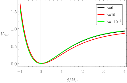
Figure 1: Plot of potential $V_{Nor}$ normalized by $\kappa_{\alpha}M_{P}^{2}/4$ as a function of $\phi/M_{p}$. The three curves were obtained with $b=0$ (black), $b=-10^{-2}$ (green) e $b=10^{-1}$ (red). The choice of $b=-10^{-2}$ comes from the fact that negative $b$ must respect the constraint $b>-e^{-\chi}$.

The most significant difference occurs for $b=10^{-1}$, but even in this case, the curve behaves similarly to the Starobinsky potential. Thus, it is clear that we have a slow-roll inflationary regime in the plateau region. Moreover, for $b\neq 0$, the minimum of the potential shifts to a value different from the origin:

$$V^{\prime}\left(\phi\right)=0\Rightarrow\chi\left(\phi_{\min}\right)=0$$

which, by the equation (3.20), results in

$$\phi_{\min}=M_{P}\sqrt{6}\left[\sqrt{1+b}-1-\ln\left(\frac{1+\sqrt{1+b}}{2}\right)\right].$$ (4.6)

For the particular cases $b=10^{-1}$ and $b=-10^{-2}$, we obtain $\phi_{\min}\approx 0.0605$ $M_{P}$ and $\phi_{\min}\approx-0.0061$ $M_{P}$, respectively. Despite this change, in the neighborhoods of $\phi_{\min}$, the potential behaves like a quadratic potential $V\left(\phi\right)\sim\left(\phi-\phi_{\min}\right)^{2}$. Therefore, at the end of the inflationary regime, the period of coherent oscillations produces a cosmic dynamic identical to the Starobinsky model, i.e. an effective equation of state $\left\langle w\right\rangle\approx 0$ and a period of expansion like a matter-dominated universe [3].

4.1 Slow-roll regime

The slow-roll inflationary regime occurs in the plateau region of the potential where $\dot{\phi}^{2}\ll V\left(\phi\right)$. In this region, the equations (4.1), (4.2) and (4.3) can be approximated by

$$H^{2}\approx\frac{V}{3M_{P}^{2}}\text{, \ }\frac{\dot{\phi}}{M_{P}}\approx-\frac{V^{\prime}}{\sqrt{3V}}\text{ \ and\ \ }\dot{H}\approx-\frac{V^{\prime 2}}{6V}.$$ (4.7)

Let’s start by calculating the number of e-folds $N$ in slow-roll leading-order. Using the Eqs. (4.7) and (3.17) we get

$$N\equiv\ln\left(\frac{a_{end}}{a}\right)\approx-\frac{1}{M_{P}^{2}}{\displaystyle\int\limits_{\phi}^{\phi_{end}}}\frac{V\left(\phi\right)}{V^{\prime}\left(\phi\right)}d\phi\approx-\frac{3}{4}{\displaystyle\int\limits_{\chi}^{\chi_{end}}}\left[be^{2\chi}+e^{\chi}\left(1-b\right)-1\right]d\chi.$$

Integrating this last expression and considering $\left|b\right|<10^{-1}$ and $e^{\chi}\gg e^{\chi_{end}}$ we obtain

$$N\approx\frac{3}{4}e^{\chi}\left(1+\frac{b}{2}e^{\chi}\right).$$ (4.8)

By imposing the Starobinsky limit, the equation (4.8) can be uniquely inverted. Thus,

$$e^{\chi}=\frac{\sqrt{1+\frac{8}{3}bN}-1}{b}.$$ (4.9)

Note that for $b<0$, we have an extra constraint given by $8bN>-3$. Hence, the $b$ parameter is limited by the range

$$-\frac{3}{8N}<b<0.1.$$ (4.10)

For a maximum of $60$ e-folds, we get $-0.00625<b<0.1$.

The next step is to compute the slow-roll parameters $\epsilon$ and $\eta$ defined as

$$\epsilon\equiv-\frac{\dot{H}}{H^{2}}\text{ \ \ and \ \ }\eta\equiv-\frac{1}{H}\frac{\dot{\epsilon}}{\epsilon}.$$

In slow-roll leading-order, these parameters can be written in terms of the potential and its derivatives:

$$\text{ }\epsilon\approx\frac{M_{P}^{2}}{2}\left(\frac{V^{\prime}\left(\phi\right)}{V\left(\phi\right)}\right)^{2}\text{ \ \ and \ \ }\eta\approx 2M_{p}^{\text{ }2}\left[\frac{V^{\prime\prime}\left(\phi\right)}{V\left(\phi\right)}-\left(\frac{V^{\prime}\left(\phi\right)}{V\left(\phi\right)}\right)^{2}\right].$$

By carrying out the explicit calculations, we get

$$\epsilon\approx\frac{4}{3}\left(\frac{e^{-2\chi}}{1+be^{\chi}}\right)\text{ \ \ and \ \ }\eta\approx-\frac{4}{3}e^{-\chi}\left(\frac{2+3be^{\chi}}{\left(1+be^{\chi}\right)^{2}}\right).$$

Finally, substituting Eq. (4.9) in these two expressions and performing the suitable approximations, we obtain

$$\epsilon\approx\frac{4}{3}\left[\frac{b^{2}}{\left(\sqrt{1+\frac{8}{3}bN}-1\right)^{2}\sqrt{1+\frac{8}{3}bN}}\right]\text{ \ and \ }\eta\approx-\frac{4b}{3}\left[\frac{3\sqrt{1+\frac{8}{3}bN}-1}{\left(\sqrt{1+\frac{8}{3}bN}-1\right)\left(1+\frac{8}{3}bN\right)}\right].$$ (4.11)

Note that in the limit $b\rightarrow 0$, we recover the results of the Starobinsky model i.e.

$$\lim_{b\rightarrow 0}\epsilon=\frac{3}{4}\frac{1}{N^{2}}\text{ \ \ and \ \ }\lim_{b\rightarrow 0}\eta=-\frac{2}{N}\text{.}$$

The equations (4.11) ensure a slow-roll inflationary regime, i.e. $\epsilon\ll 1$ and $\eta\ll 1$, whenever we have a sufficiently large number of e-folds (e.g. $N\geq 50$).

4.2 Observational constraints

Inflationary models can be constrained from observations of CMB anisotropies. The constraint procedure is performed from the scalar and tensor power spectra parameterized as [60]

$$\mathcal{P}_{s}=A_{s}\left(\frac{k}{k_{\ast}}\right)^{n_{s}}\text{ \ \ and \ \ \ }\mathcal{P}_{t}=A_{t}\left(\frac{k}{k_{\ast}}\right)^{n_{t}},$$ (4.12)

where $A_{s}$ and $A_{t}$ are the scalar and tensor amplitudes, $n_{s}$ and $n_{t}$ are the scalar and tensor spectral indices, and $k_{\ast}$ is a reference scale (pivot scale). It is also usual to define the tensor-to-scalar ratio

$$r\equiv\frac{A_{t}}{A_{s}}.$$ (4.13)

Moreover, for inflationary models of a single canonical scalar field (such as the proposed model in its approximate form), the consistency relation $n_{t}=-r/8$ is always verified. Thus, there are only three free parameters that can be represented by $A_{s}$, $n_{s}$ and $r$.

In slow-roll leading-order, we know that [61, 62]

$$n_{s}=1+\eta-2\epsilon\text{ \ \ and \ \ }r=16\epsilon.$$ (4.14)

From Eqs. (4.11) we see that $n_{s}$ and $r$ depend on the number of e-folds $N$ and the parameter $b$.

The comparison with the observations through the parameter space $n_{s}\times r$ must be performed by separating the cases of $b$ positive and $b$ negative. Figures 2 and 3 show the cases $b<0$ and $b>0$, respectively.

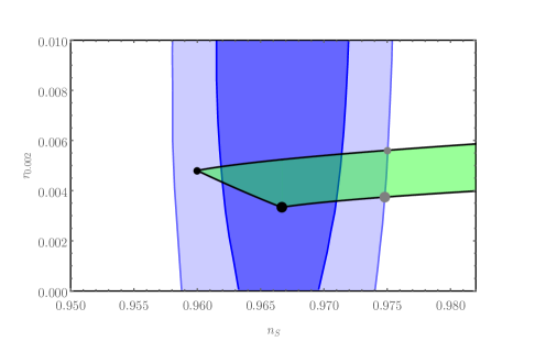
Figure 2: Parameter space $n_{s}\times r$ which include the observational constraints $68\%$ (dark blue) and $95\%$ (light blue) C.L. [14] and the theoretical evolution of the model (green) calculated from Eq. (4.14). The constraint is made considering $b<0$ and $50\leq N\leq 60$. The black circles represent the Starobinsky model ($b=0$) for $N=50$ (smaller one) and $N=60$ (bigger one). As $\left|b\right|$ increases the curves move to the right (light green region) increasing the tensor-to-scalar ratio and the scalar tilt values. The grey circles take into account the maximum values of $\left|b\right|$ still consistent with the region of $95\%$ C.L.. In this case, $N=50$ and $N=60$ correspond to $b=-0.0060$ and $b=-0.0047$, respectively.

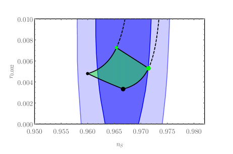
Figure 3: Similar analyzes as figure 2 but now considering $b>0$. The green circles correspond to the upper bound $b=10^{-1}$ where the perturbative approach is still valid. In this case, $N=50$ and $N=60$ correspond to $\left(n_{s},r\right)=\left(0.9654,0.0073\right)$ and $\left(n_{s},r\right)=\left(0.9714,0.0053\right)$, respectively. The dotted lines extrapolate Eq. (4.14) to $b>10^{-1}$.

Figure 2 shows that for negative $b$, the observational data constrain in a very restrictive way the value of $b$. Within $50\leq N\leq 60$, we get $-0.006\leq b<0$. In addition, the variation of $b$ has little effect on the value of the tensor-to-scalar ratio. For $N=50$ and $N=60$ within $95\%$ C.L., we obtain $0.0048<r<0.0056$ and $0.0033<r<0.0037$, respectively.

On the other hand, from figure 3, we see that the value of positive $b$ is little constrained by the observations. The entire region encompassing $0<b\leq 10^{-1}$ and $50\leq N\leq 60$ is within the range of observationally values allowed by $95\%$ C.L.. Moreover, we realize that $b$ positive admits a more significant variation of the tensor-to-scalar ratio than $b$ negative.

In addition to the restrictions on parameters $b$ and $N$, we can constrain the parameter $\kappa_{\alpha}$ from the observation of the scalar amplitude $A_{s}$. In slow-roll leading-order, the scalar amplitude can be written as [61, 62]

$$A_{s}=\frac{1}{12\pi^{2}M_{p}^{6}}\frac{V^{3}}{V^{\prime 2}}.$$ (4.15)

Substituting Eqs. (4.4), (4.5) and (4.9) in the last expression, we get

$$\kappa_{\alpha}=\frac{2^{7}\pi^{2}A_{s}M_{p}^{2}b^{2}}{\left(\sqrt{1+\frac{8}{3}bN}-1\right)^{2}\sqrt{1+\frac{8}{3}bN}}.$$ (4.16)

Using Eqs. (4.11) and (4.14) and the value $A_{s}=2.1\times 10^{-9}$ [63], we can rewrite $\kappa_{\alpha}$ as

$$\kappa_{\alpha}=6\pi^{2}rA_{s}M_{p}^{2}=1.25\times 10^{-7}rM_{p}^{2}.$$ (4.17)

Therefore, taking into account that the maximum variation of the tensor-to-scalar ratio is $0.0033\leq r\leq 0.0073$, we obtain

$$4\times 10^{-10}M_{p}^{2}\leq\kappa_{\alpha}\leq 9\times 10^{-10}M_{p}^{2}.$$ (4.18)

The last result confirms that the inflation energy scale $E_{\inf}\sim\kappa_{\alpha}^{1/2}\sim 10^{-5}$ $M_{p}$.

5 Final Comments

In this work, we investigate how the inclusion of a nonlocal term $R\ln\left(\square\right)R$ changes the Starobinsky inflation. We consider that this term provides a small correction to the Starobinsky model. Using a perturbative approach, we show that the field equations reduce to local equations, which in the Einstein frame can be described by a canonical scalar field minimally coupled to general relativity. The $b$ parameter, which measures the effectiveness of the nonlocal term concerning the Starobinsky term, was constrained in Section 4.2. For negative $b$ we obtained $\left|b\right|<0.006$, and for positive $b$ we did not obtain any constraint within the perturbative context. The results achieved in Section 4.2 are similar to those presented in Refs. [59, 64], where the authors study the influence of the $R\square R$ term on Starobinsky inflation. This similarity shows that in the context of small corrections, the contribution of the nonlocal term occurs essentially through the first term of the series in Eq. (2.2).

The proposed model is inserted in a context of effective theories whose validity energy range is below the Planck scale and far above the masses of the matter fields. In this context, the $b$ parameter is not a free parameter but depends on the quantity of matter scalar fields present in the original theory. If we take into account only the Higgs field and fix the renormalization point on the inflationary energy scale ($\mu^{2}\sim\kappa_{0}$), we get, from Eqs. (2.8) and (4.18),

$$\left|b\right|=\frac{4\kappa_{0}}{M_{P}^{2}}\frac{20\left(6\xi-1\right)^{2}}{11520\pi^{2}}\sim 10^{-13}\left(6\xi-1\right)^{2},$$

where $\kappa_{0}\simeq\kappa_{\alpha}\simeq 5\times 10^{-10}M_{p}^{2}$. This equation shows that for $\left|b\right|\sim 10^{-3}$ (see figure 2), it is necessary $\xi\sim 2\times 10^{4}$. The high value of the non-minimum coupling constant $\xi$ is consistent with the Higgs inflation model proposed in [15] where $\xi\sim 5\times 10^{4}\sqrt{\lambda}$. It is also worth mentioning that the inclusion of new scalar degrees of freedom increases the value of $N_{s}$ present in Eq. (2.8) and causes $\xi$ to decrease to a fixed value of $b$.

The discussion in the previous paragraph supports the idea that two different approaches can be used to deal with light matter fields in an inflationary context of modified gravity. The first approach considers these fields explicitly and analyzes how they affect inflation (see, for example, ref. [66]). The second one uses the idea of effective theories, which treat all matter fields collectively and transfer their effects to the gravitational degrees of freedom. In principle, the second approach is only correct if the second nonlocal term $\left(2\beta/M_{P}^{2}\right)C_{\kappa\rho\alpha\beta}\ln\left(\square\right)C^{\kappa\rho\alpha\beta}$ is also included. Nevertheless, only considering matter fields of the standard model (minimalist model), the value of $c\equiv$ $4\beta\kappa_{0}/M_{P}^{2}$, which measures the effectiveness of the second nonlocal term concerning the Starobinsky term, is extremely small ($\left|c\right|\sim 10^{-8}$) [24]. Thus, unless the matter degrees of freedom increase by several orders of magnitude, it is reasonable to expect that the term $C_{\kappa\rho\alpha\beta}\ln\left(\square\right)C^{\kappa\rho\alpha\beta}$ will be negligible in the inflationary context.

The conclusion presented above disregards the inclusion of new degrees of freedom arising from the nonlocal term. It occurs because the approximation of small corrections performed in section 3 transfers any extra degrees of freedom to the scalaron associated with the $R^{2}$ term. In this sense, possible issues generated by new degrees of freedom are being neglected. For example, it is common for degrees of freedom engendered by higher-order models to present ghost-like fields. Even so, the possible pathologies associated with these fields do not necessarily influence the inflationary dynamics. A situation where this statement is true occurs in the local model $\mathcal{L}=R+aR^{2}+bR\square R$. In this model, the term $R\square R$ contributes an extra ghost field, but the perturbations of this field are negligible in the inflationary context [64]. It is also worth mentioning that the results found in Ref. [64] are similar to those obtained in Ref. [59] where the authors consider only small corrections of $R\square R$ to the Starobinsky model. Due to its nonlocal feature, the study of extra degrees of freedom generated by the term $R\ln\left(\square\right)R$ is more complex than that performed in local models. This study will be carried out in future works.

Appendix A Jordan Frame

In order to rewrite the gravitational action (2.1) in the Jordan frame, we start by defining two parameters

$$\lambda_{1}=R\text{ \ \ \ and \ \ \ }\lambda_{2}=\ln\left(\frac{\square}{\mu^{2}}\right)R\text{.}$$

From these parameters, we build a new action in the form

$$\bar{S}=\frac{M_{P}^{2}}{2}\int d^{4}x\sqrt{-g}\left\{\lambda_{1}+\frac{1}{2\kappa_{0}}\lambda_{1}^{2}+\frac{2\alpha}{M_{P}^{2}}\lambda_{1}\lambda_{2}\theta_{1}\left(R-\lambda_{1}\right)+\theta_{2}\left[\ln\left(\frac{\square}{\mu^{2}}\right)\lambda_{1}-\lambda_{2}\right]\right\},$$

where the fields $\theta_{1}$ and $\theta_{2}$ are Lagrange multipliers. By taking the variation of $\bar{S}$ concerning $\theta_{1}$ and $\theta_{2}$ and using the field equations, we easily realize that $\bar{S}$ and the original action are equivalent on-shell.

The next step is to compute the variation of $\bar{S}$ with respect to $\lambda_{1}$ and $\lambda_{2}$. To perform this calculation, we will use the series representation (2.2). Thus,

$$\int d^{4}x\sqrt{-g}\theta_{2}\ln\left(\frac{\square}{\mu^{2}}\right)\lambda_{1}=\sum_{n=1}^{\infty}\sum_{k=0}^{n}\frac{\left(-1\right)^{n-1}}{\mu^{2k}n}\frac{\left(-1\right)^{n-k}n!}{k!\left(n-k\right)!}\int d^{4}x\sqrt{-g}\theta_{2}\square^{k}\lambda_{1}.$$

Applying Leibniz rule $k$ times in $\theta_{2}\square^{k}\lambda_{1}$ and neglecting the surface terms we get

$$S=\frac{M_{P}^{2}}{2}\int d^{4}x\sqrt{-g}\left\{\lambda_{1}+\frac{1}{2\kappa_{0}}\lambda_{1}^{2}+\frac{2\alpha}{M_{P}^{2}}\lambda_{1}\lambda_{2}+\theta_{1}\left(R-\lambda_{1}\right)+\lambda_{1}\ln\left(\frac{\square}{\mu^{2}}\right)\theta_{2}-\theta_{2}\lambda_{2}\right\}.$$ (A.1)

Thereby, the variations concerning $\lambda_{1}$ and $\lambda_{2}$ of the above expression result in the field equations

$$1+\frac{1}{\kappa_{0}}\lambda_{1}+\frac{2\alpha}{M_{P}^{2}}\lambda_{2}-\theta_{1}+\ln\left(\frac{\square}{\mu^{2}}\right)\theta_{2} =0,$$

$$\frac{2\alpha}{M_{P}^{2}}\lambda_{1}-\theta_{2} =0.$$

By inverting the last equations for $\lambda_{1}$ and $\lambda_{2}$ and substituting the result in Eq. (A.1) we obtain

$$S=\frac{M_{P}^{2}}{2}\int d^{4}x\sqrt{-g}\left\{\theta_{1}R+\frac{M_{P}^{2}}{2\alpha}\left(1-\theta_{1}\right)\theta_{2}+\frac{1}{2\kappa_{0}}\left(\frac{M_{P}^{2}}{2\alpha}\right)^{2}\theta_{2}^{2}+\frac{M_{P}^{2}}{2\alpha}\theta_{2}\ln\left(\frac{\square}{\mu^{2}}\right)\theta_{2}\right\}.$$ (A.2)

Finally, we define

$$\theta=\theta_{1}\text{, \ \ \ }\theta_{2}=\frac{2\alpha\kappa_{0}}{M_{P}^{2}}\lambda\text{ \ \ \ and \ \ \ }b=\frac{4\alpha\kappa_{0}}{M_{P}^{2}},$$

and we achieve the equation (2.7), which represents the original action in the Jordan frame.

Appendix B Metric equation in Jordan frame

We start by taking the variation $\delta_{g}$ in the action (2.11) concerning $g^{\mu\nu}$:

$$\delta_{g}S=\frac{M_{P}^{2}}{2}\left\{\int d^{4}x\sqrt{-g}\left[\theta\delta_{g}R-\frac{1}{2}\left[\theta R+\kappa_{0}\left(1-\theta\right)\lambda+\frac{\kappa_{0}}{2}\lambda^{2}\right]g_{\mu\nu}\delta g^{\mu\nu}\right]+\delta_{g}S_{NL}\right\},$$ (B.1)

where [67]

$$\int d^{4}x\sqrt{-g}\theta\delta_{g}R=\int d^{4}x\sqrt{-g}\left[\theta R_{\mu\nu}+\left(\square\theta\right)g_{\mu\nu}-\left(\nabla_{\mu}\nabla_{\nu}\theta\right)\right]\delta_{g}g^{\mu\nu}.$$ (B.2)

Let’s compute

$$\delta_{g}S_{NL}=\frac{M_{P}^{2}\kappa_{0}b}{4}\sum_{n=1}^{\infty}\sum_{k=0}^{n}\frac{\left(-1\right)^{n-1}}{n}\frac{\left(-1\right)^{n-k}n!}{k!\left(n-k\right)!}\frac{1}{\mu^{2k}}\delta_{g}\int d^{4}x\sqrt{-g}\lambda\left(\square^{k}\lambda\right).$$ (B.3)

The first step is to expand $\square^{k}$ as

$$\square^{k}=\nabla_{\nu_{1}}\nabla^{\nu_{1}}\nabla_{\nu_{2}}\nabla^{\nu_{2}}...\nabla_{\nu_{k-1}}\nabla^{\nu_{k-1}}\nabla_{\nu_{k}}\nabla^{\nu_{k}}.$$

Thus,

$$\delta_{g}\int d^{4}x\sqrt{-g}\lambda\left(\square^{k}\lambda\right) =\delta_{g}\int d^{4}x\sqrt{-g}\lambda\nabla_{\nu_{1}}\nabla^{\nu_{1}}\nabla_{\nu_{2}}\nabla^{\nu_{2}}...\nabla_{\nu_{k-1}}\nabla^{\nu_{k-1}}\nabla_{\nu_{k}}\nabla^{\nu_{k}}\lambda$$

$$=\int d^{4}x\left(\delta_{g}\sqrt{-g}\right)\lambda\left(\square^{k}\lambda\right)$$

$$+\int d^{4}x\sqrt{-g}\lambda\left[\delta_{g}\left(\nabla_{\nu_{1}}\nabla^{\nu_{1}}\right)\right]\nabla_{\nu_{2}}\nabla^{\nu_{2}}...\nabla_{\nu_{k-1}}\nabla^{\nu_{k-1}}\nabla_{\nu_{k}}\nabla^{\nu_{k}}\lambda$$

$$+\int d^{4}x\sqrt{-g}\lambda\nabla_{\nu_{1}}\nabla^{\nu_{1}}\left[\delta_{g}\left(\nabla_{\nu_{2}}\nabla^{\nu_{2}}\right)\right]...\nabla_{\nu_{k-1}}\nabla^{\nu_{k-1}}\nabla_{\nu_{k}}\nabla^{\nu_{k}}\lambda+...$$

$$+\int d^{4}x\sqrt{-g}\lambda\nabla_{\nu_{1}}\nabla^{\nu_{1}}\nabla_{\nu_{2}}\nabla^{\nu_{2}}...\left[\delta_{g}\left(\nabla_{\nu_{k-1}}\nabla^{\nu_{k-1}}\right)\right]\nabla_{\nu_{k}}\nabla^{\nu_{k}}\lambda$$

$$+\int d^{4}x\sqrt{-g}\lambda\nabla_{\nu_{1}}\nabla^{\nu_{1}}\nabla_{\nu_{2}}\nabla^{\nu_{2}}...\nabla_{\nu_{k-1}}\nabla^{\nu_{k-1}}\left[\delta_{g}\left(\nabla_{\nu_{k}}\nabla^{\nu_{k}}\right)\lambda\right].$$

Integrating by parts several times, we get

$$\delta_{g}\int d^{4}x\sqrt{-g}\lambda\left(\square^{k}\lambda\right) =\int d^{4}x\left(\delta_{g}\sqrt{-g}\right)\lambda\left(\square^{k}\lambda\right)+\int d^{4}x\sqrt{-g}\lambda\left[\delta_{g}\left(\nabla_{\nu_{1}}\nabla^{\nu_{1}}\right)\right]\square^{k-1}\lambda$$

$$+\int d^{4}x\sqrt{-g}\left[\square\lambda\right]\left[\delta_{g}\left(\nabla_{\nu_{2}}\nabla^{\nu_{2}}\right)\right]\square^{k-2}\lambda+...$$

$$+\int d^{4}x\sqrt{-g}\left[\square^{k-2}\lambda\right]\left[\delta_{g}\left(\nabla_{\nu_{k-1}}\nabla^{\nu_{k-1}}\right)\right]\square\lambda$$

$$+\int d^{4}x\sqrt{-g}\left[\square^{k-1}\lambda\right]\left[\delta_{g}\left(\nabla_{\nu_{k}}\nabla^{\nu_{k}}\right)\right]\lambda.$$

In compact notation, the above expression can be written as

$$\delta_{g}\int d^{4}x\sqrt{-g}\lambda\left(\square^{k}\lambda\right)=\int d^{4}x\left(\delta_{g}\sqrt{-g}\right)\lambda\left(\square^{k}\lambda\right)+{\displaystyle\sum\limits_{l=1}^{k}}I_{l,k},$$

where

$$I_{l,k}=\int d^{4}x\sqrt{-g}\square^{l-1}\lambda\left[\delta_{g}\left(\nabla_{\nu}\nabla^{\nu}\right)\square^{k-l}\lambda\right].$$

The next step is working with the integral $I_{l,k}$. Using the relation $\delta\sqrt{-g}=-\frac{1}{2}\sqrt{-g}g_{\mu\nu}\delta g^{\mu\nu}$, we obtain

$$I_{l,k} =\int d^{4}x\sqrt{-g}\square^{l-1}\lambda\left[\delta_{g}\left(\frac{1}{\sqrt{-g}}\partial_{\mu}\left(\sqrt{-g}g^{\mu\nu}\partial_{v}\right)\right)\square^{k-l}\lambda\right]$$

$$=\frac{1}{2}\int d^{4}x\sqrt{-g}\left(\square^{l-1}\lambda\right)\left(\square^{k-l+1}\lambda\right)g_{\mu\nu}\delta_{g}g^{\mu\nu}$$

$$+\frac{1}{2}\int d^{4}x\sqrt{-g}\left[\nabla_{\rho}\square^{l-1}\lambda\right]\left[\nabla^{\rho}\square^{k-l}\lambda\right]g_{\mu\nu}\delta_{g}g^{\mu\nu}$$

$$-\int d^{4}x\sqrt{-g}\left[\nabla_{\mu}\square^{l-1}\lambda\right]\left[\nabla_{v}\square^{k-l}\lambda\right]\delta_{g}g^{\mu\nu}.$$

Thus,

$$\delta_{g}\int d^{4}x\sqrt{-g}\lambda\left(\square^{k}\lambda\right) =-\frac{1}{2}\int d^{4}x\sqrt{-g}\lambda\left(\square^{k}\lambda\right)g_{\mu\nu}\delta g^{\mu\nu}$$

$$+{\displaystyle\sum\limits_{l=1}^{k}}\frac{1}{2}\int d^{4}x\sqrt{-g}\left(\square^{l-1}\lambda\right)\left(\square^{k-l+1}\lambda\right)g_{\mu\nu}\delta g^{\mu\nu}$$

$$+{\displaystyle\sum\limits_{l=1}^{k}}\frac{1}{2}\int d^{4}x\sqrt{-g}\left[\nabla_{\rho}\square^{l-1}\lambda\right]\left[\nabla^{\rho}\square^{k-l}\lambda\right]g_{\mu\nu}\delta g^{\mu\nu}$$

$$-{\displaystyle\sum\limits_{l=1}^{k}}\int d^{4}x\sqrt{-g}\left[\nabla_{\mu}\square^{l-1}\lambda\right]\left[\nabla_{v}\square^{k-l}\lambda\right]\delta_{g}g^{\mu\nu}.$$

By substituting this last result in Eq. (B.3), we get

$$\delta_{g}S_{NL} =-\frac{b\kappa_{0}}{4}\int d^{4}x\sqrt{-g}\delta g^{\mu\nu}g_{\mu\nu}\lambda\ln\left(\frac{\square}{\mu^{2}}\right)\lambda$$

$$+\frac{b\kappa_{0}}{4}\int d^{4}x\sqrt{-g}\delta g^{\mu\nu}g_{\mu\nu}\sum_{n=1}^{\infty}\sum_{k=1}^{n}\frac{\left(-1\right)^{n-1}}{n}\frac{\left(-1\right)^{n-k}n!}{k!\left(n-k\right)!}\frac{1}{\mu^{2k}}{\displaystyle\sum\limits_{l=1}^{k}}\left(\square^{l-1}\lambda\right)\left(\square^{k-l+1}\lambda\right)$$

$$+\frac{b\kappa_{0}}{4}\int d^{4}x\sqrt{-g}\delta g^{\mu\nu}g_{\mu\nu}\sum_{n=1}^{\infty}\sum_{k=1}^{n}\frac{\left(-1\right)^{n-1}}{n}\frac{\left(-1\right)^{n-k}n!}{k!\left(n-k\right)!}\frac{1}{\mu^{2k}}{\displaystyle\sum\limits_{l=1}^{k}}\left[\nabla_{\rho}\square^{l-1}\lambda\right]\left[\nabla^{\rho}\square^{k-l}\lambda\right]$$

$$-\frac{b\kappa_{0}}{2}\int d^{4}x\sqrt{-g}\delta_{g}g^{\mu\nu}\sum_{n=1}^{\infty}\sum_{k=1}^{n}\frac{\left(-1\right)^{n-1}}{n}\frac{\left(-1\right)^{n-k}n!}{k!\left(n-k\right)!}\frac{1}{\mu^{2k}}{\displaystyle\sum\limits_{l=1}^{k}}\left[\nabla_{\mu}\square^{l-1}\lambda\right]\left[\nabla_{v}\square^{k-l}\lambda\right].$$ (B.4)

Finally, we substitute Eqs. (B.2) and (B.4) in Eq. (B.1), and we achieve the metric equation (2.12).

References

[1]A. H. Guth, The inflationary universe: a possible
solution to the horizon and flatness problems, Phys. Rev. D 23, 347 (1981).
[2]A. D. Linde, Chaotic inflation, Phys. Lett.
B 129 (1983) 177.
[3]V. Mukhanov, Physical Foundations of Cosmology,
Cambridge University Press, 2005.
[4]J. Martin, C. Ringeval and V. Vennin,
Encyclopædia inflationaris, Physics of the Dark Universe
5-6, 75 (2014), arXiv:1303.3787 [astro-ph.CO].
[5]K. Bamba, R. Myrzakulov, S. D. Odintsov and L. Sebastiani,
Trace-anomaly driven inflation in modified gravity and the BICEP2 result,
Phys. Rev. D 90, 043505 (2014), arXiv:1403.6649 [hep-th].
[6]R. Myrzakulov, S. D. Odintsov and L. Sebastiani,
Inflationary universe from higher-derivative quantum gravity,
Phys. Rev. D 91, 083529 (2015), arXiv:1412.1073 [gr-qc].
[7]E. Elizalde, S. D. Odintsov, L. Sebastiani and R.Myrzakulov,
Beyond-one-loop quantum gravity action yielding both inflation and late-time acceleration,
Nucl. Phys. B 921, 411 (2017), arXiv:1706.01879 [gr-qc].
[8]A. S. Koshelev, L. Modesto, L. Rachwal, A. A. Starobinsky,
Occurrence of exact inflation in non-local UV-complete gravity,
J. High Energ. Phys. 11, 67 (2016), arXiv:1604.03127 [hep-th].
[9]A. S. Koshelev, K. S. Kumar, A. A. Starobinsky,
inflation to probe non-perturbative quantum gravity,
J. High Energ. Phys. 03, 71 (2018), arXiv:1711.08864 [hep-th].
[10]A. S. Koshelev, K. S. Kumar, A. Mazumdar and A. A. Starobinsky,
Non-Gaussianities and tensor-to-scalar ratio in non-local -like inflation,
J. High Energ. Phys. 06, 152 (2020), arXiv:2003.00629 [hep-th].
[11]A. S. Koshelev, K. S. Kumar and A. A. Starobinsky,
Analytic infinite derivative gravity, -like inflation, quantum
gravity and CMB, Int. J. Mod. Phys. D. 29, 2043018 (2020), arXiv:2005.09550 [hep-th].
[12]R. Brandenberger, Initial conditions for inflation
- A short review, Int. J. Mod. Phys. D 26, 1740002 (2017),
arXiv:1601.01918 [hep-th].
[14]BICEP and Keck collaborations, BICEP/Keck XIII: Improved
Constraints on Primordial Gravitational Waves using Planck, WMAP, and
BICEP/Keck Observations through the 2018 Observing Season, Phys. Rev. Lett.
127, 151301 (2021), arXiv:2110.00483 [astro-ph.CO].
[15]F. L. Bezrukov and M. Shaposhnikov, The
standard model Higgs boson as the inflaton, Phys. Lett. B 659, 703
(2008), arXiv:0710.3755 [hep-th].
[16]A. Starobinsky, A new type of isotropic cosmological
models without singularity, Phys. Lett. B 91, 99 (1980).
[17]C. G. Callan, Jr., S. R. Coleman and R. Jackiw, A
new improved energy - momentum tensor, Annals Phys. 59, 42 (1970).
[18]C. P. Burgess, H. M. Lee and M. Trott,
Power-counting and the validity of the classical approximation during
inflation, J. High Energy Phys. 9, 103 (2009), arXiv:0902.4465 [hep-ph].
[19]M. P. Hertzberg, On inflation with non-minimal
coupling, J. High Energy Phys. 11, 23 (2010), arXiv:1002.2995 [hep-ph].
[21]T. Markkanena, A. Rajantieb and S. Stopyrac,
Cosmological aspects of Higgs vacuum metastability, Front. Astron.
Space Sci. 5, 40 (2018), arXiv:1809.06923 [astro-ph.CO].
[22]A. O. Barvinsky and G. A. Vilkovisky, The
generalized Schwinger-Dewitt technique in gauge theories and quantum gravity,
Phys. Rep. 119, 1 (1985).
[23]I. L. Buchbinder, S. D. Odintsov and I. L. Shapiro,
Effective Action in Quantum Gravity, IOP Publishing, Bristol, 1992.
[24]J. F. Donoghue and B. K. El-Menoufi, Non-local
quantum effects in cosmology 1: Quantum memory, non-local FLRW equations and
singularity avoidance, Phys. Rev. D 89, 104062 (2014),
arXiv:1402.3252 [gr-qc].
[25]M. Maggiore, Nonlocal infrared modifications of
gravity. A review, Fundam. Theor. Phys. 187, 221 (2017),
arXiv:1606.08784 [hep-th].
[26]P. M. Teixeira, I. L. Shapiro and T. G. Ribeiro,
One-loop effective action: nonlocal form factors and renormalization
group, Grav. Cosmol. 26, 185 (2020), arXiv:2003.04503 [hep-th].
[27]G.’t Hooft and M. J. G. Veltman, One loop
divergencies in the theory of gravitation, Ann. Inst. H. Poincare Phys.Theor.
A 20, 69 (1974).
[28]K. S. Stelle, Renormalization of
higher-derivative quantum gravity, Phys. Rev. D 16, 953 (1977).
[29]A. Pais and G. E. Uhlenbeck, On field theories with
non-localized action, Phys. Rev. 79, 145 (1950).
[30]T. D. Lee and G. C. Wick, Negative metric and
the unitarity of the S matrix, Nucl. Phys. B 9, 209 (1969).
[31]A. Salvio and A. Strumia, Quantum mechanics of
4-derivative theories, Eur. Phys. J. C 76, 227 (2016),
arXiv:1512.01237 [hep-th].
[32]C. M. Bender and P. D. Mannheim, No-ghost theorem
for the fourth-order derivative Pais-Uhlenbeck oscillator model, Phys. Rev.
Lett. 100, 110402 (2008), arXiv:0706.0207 [hep-th].
[33]C. M. Bender and P. D. Mannheim, Exactly solvable
PT-symmetric Hamiltonian having no Hermitian counterpart, Phys. Rev. D
78, 025022 (2008), arXiv:0804.4190 [hep-th].
[34]L. Modesto and I. L. Shapiro, Superrenormalizable
quantum gravity with complex ghosts, Phys. Lett. B 755, 279 (2016),
arXiv:1512.07600 [hep-th].
[35]J. F. Donoghue and G. Menezes, Unitarity, stability
and loops of unstable ghosts, Phys. Rev. D 100, 105006 (2019),
arXiv:1908.02416 [hep-th].
[36]D. Anselmi, On the quantum field theory of the
gravitational interactions, J. High Energy Phys. 6, 086 (2017),
arXiv:1704.07728 [hep-th].
[37]D. Anselmi and M. Piva, The Ultraviolet behavior
of quantum gravity, J. High Energy Phys. 5, 27 (2018),
arXiv:1803.07777 [hep-th].
[38]A. Salvio, Quasi-Conformal Models and the Early Universe,
Eur. Phys. J. C 79, 750 (2019), arXiv:1907.00983 [hep-ph].
[39]A. Salvio, Dimensional Transmutation in Gravity and Cosmology,
Int. J. Mod. Phys. A 36, 2130006 (2021), arXiv:2012.11608 [hep-th].
[40]M. M. Ivanov and A. A. Tokareva, Cosmology with a
light ghost, J. Cosmol. Astropart. Phys. 12, 18 (2016),
arXiv:1610.05330 [hep-th].
[41]A. Salvio, Inflationary perturbations in no-scale
theories, Eur. Phys. J. C 77, 267 (2017), arXiv:1703.08012 [astro-ph.CO].
[42]D. Anselmi, E. Bianchi and M. Piva, Predictions
of quantum gravity in inflationary cosmology: effects of the Weyl-squared
term, J. High Energy Phys. 7, 211 (2020), arXiv:2005.10293 [hep-th].
[43]L. Kofman, A. D. Linde and A. A. Starobinsky,
Towards the theory of reheating after inflation, Phys. Rev. D
56, 3258 (1997), arXiv:hep-ph/9704452.
[44]B. A. Bassett, S. Tsujikawa and D. Wands,
Inflation dynamics and reheating, Rev. Mod. Phys. 78, 537
(2006), arXiv:astro-ph/0507632.
[45]K. D. Lozanov, Lectures on reheating after
inflation, (2019), arXiv:1907.04402 [astro-ph.CO].
[46]J. F. Donoghue, M. M. Ivanov and A. Shkerin,
EPFL lectures on general relativity as a quantum field theory,
(2017), arXiv:1702.00319 [hep-th].
[47]X. Calmet, R. Casadio and F. Kuipers, Quantum
gravitational corrections to a star metric and the black hole limit, Phys.
Rev. D 100, 086010 (2019), arXiv:1909.13277 [hep-th].
[48] T. Biswas, A. Mazumdar and W. Siegel, Bouncing
Universes in String-inspired Gravity, J. Cosmol. Astropart. Phys. 3, 9 (2006),
arXiv:hep-th/0508194.
[49] T. Biswas, T. Koivisto and A. Mazumdar, Towards a Resolution
of the Cosmological Singularity in Non-local Higher Derivative Theories of Gravity, J. Cosmol. Astropart. Phys. 11, 8 (2010), arXiv:1005.0590 [hep-th].
[50] T. Biswas, E. Gerwick, T. Koivisto and A. Mazumdar, Towards singularity
and ghost free theories of gravity, Phys. Rev. Lett. 108 (2012) 031101, arXiv:1110.5249 [gr-qc].
[51] T. Biswas, T. Koivisto and A. Mazumdar, Nonlocal theories of gravity:
the flat space propagator, (2013), arXiv:1302.0532 [gr-qc].
[52] S. Talaganis, T. Biswas and A. Mazumdar, Towards understanding
the ultraviolet behavior of quantum loops in infinite-derivative theories of gravity, Class. Quantum Grav. 32, 215017 (2015), arXiv:1412.3467 [hep-th].
[53]D. Espriu, T. Multamaki and E. C. Vagenas,
Cosmological significance of one-loop effective gravity, Phys. Lett.
B 628, 197 (2005), arXiv:gr-qc/0503033.
[54]J. A. Cabrer and D. Espriu, Secular effects on
inflation from one-loop quantum gravity, Phys. Lett. B 663, 361
(2008), arXiv:0710.0855 [gr-qc].
[55]R. R. Cuzinatto, L. G. Medeiros and P. J. Pompeia,
Higher-order modified Starobinsky inflation, J. Cosmol. Astropart.
Phys. 2, 55 (2019), arXiv:1810.08911 [gr-qc].
[56]G. Rodrigues-da-Silva and L. G. Medeiros,
Spherically symmetric solutions in higher-derivative theories of
gravity, Phys. Rev. D 101, 124061 (2020), arXiv:2004.04878 [gr-qc].
[57]S. Nojiri, S. D. Odintsov and V. K. Oikonomou,
Modified Gravity Theories on a Nutshell: Inflation, Bounce and
Late-time Evolution, Phys. Rept. 692, 1 (2017), arXiv:1705.11098 [gr-qc].
[58]R. R. Cuzinatto, C. A. M. de Melo, L. G. Medeiros and
P. J. Pompeia, theories of gravity in Einstein frame: A higher order
modified Starobinsky inflation model in the Palatini approach, Phys. Rev. D
99, 084053 (2019), arXiv:1806.08850 [gr-qc].
[59]A. R. R. Castellanos, F. Sobreira, I. L. Shapiro and
A. A. Starobinsky, On higher derivative corrections to the inflationary model, J. Cosmol. Astropart. Phys. 12, 7
(2018), arXiv:1810.07787 [gr-qc].
[62]G. Rodrigues-da-Silva, J. Bezerra-Sobrinho and L. G.
Medeiros, A higher-order extension of Starobinsky inflation: initial
conditions, slow-roll regime and reheating phase, Phys. Rev. D 105,
063504 (2022), arXiv:2110.15502 [astro-ph.CO].
[63]N. Aghanim et al., Planck 2018 results. VI.
Cosmological parameters, Astron. Astrophys. 641, A6 (2020),
arXiv:1807.06209 [astro-ph.CO].
[64] G. Rodrigues-da-Silva and L. G. Medeiros, Second-order corrections
to Starobinsky inflation, (2022), arXiv:2207.02103 [astro-ph.CO].
[65]C. F. Steinwachs, Higgs field in cosmology,
Fundam. Theor. Phys. 199, 253 (2020), arXiv:1909.10528 [hep-ph].
[66]A. Gundhi and C. F. Steinwachs, Scalaron-Higgs
inflation, Nucl. Phys. B 954, 114989 (2020), arXiv:1810.10546 [hep-th].
[67]S. Capozziello and M. De Laurentis, Extended
theories of gravity, Phys. Rept. 509, 167 (2011), arXiv:1108.6266 [gr-qc].