A Simple Discretization Scheme for Gain Matrix Conditioning

Abstract

In industrial model predictive controllers (MPCs), models generated from regression-based system identification methods typically contain small or even physically non-existent degrees of freedom. Control issues can arise when the steady-state optimizer uses these small degrees of freedom to calculate targets for plant operation due to matrix ill-conditioning. Mathematical techniques like Relative Gain Array (RGA) and Singular Value Decomposition (SVD) are helpful for analyzing controller gain interactions and identifying conditioning issues, which can be corrected relatively easily in small models. However, these techniques are difficult and tedious to apply for larger, more complex models. This paper describes a novel, non-iterative, RGA-based, binning technique for discretizing the gain matrix and quickly solving 2$\times$2 conditioning issues for any model size, while guaranteeing gain adjustments below a certain threshold. Higher order interactions are also discussed.

I INTRODUCTION

Industrial model predictive controllers (MPCs) are commonly implemented with an integrated steady-state, Linear Program (LP) optimizer to generate targets that drive the process to an economic optimum [1]. In industrial MPC projects, one of the most difficult and time-consuming steps is understanding the interaction of the steady-state model gains with the optimizer costs in the LP solution. Part of this consideration is respecting the material and energy balance of the process, and determining how much “detail” in terms of smaller gains should be built into the model.

In practice, designers must make structural decisions in the gain matrix to reconcile the model with the true process. This step relies on the designer’s process knowledge and experience, along with the usage of process data to justify any curve or gain manipulation of the model. Adjusting the gain matrix is often a balancing act between maintaining model accuracy and usability, and arbitrarily deleting or scaling gains should be avoided. A case study from Mitsubishi demonstrated how the erroneous removal of a gain element, thought to be insignificant based on engineering judgment, resulted in controller instabilities [2].

Fundamentally, there are 3 types of MV-CV (Manipulated Variable-Controlled Variable) interactions:

• Non-collinearities: MV-CV interactions that are easy to independently control

• Collinearities: MV-CV interactions that cannot be independently controlled, because the gains are collinear

• Near-collinearities: MV-CV interactions that are difficult to independently control

The non-collinear MV-CV interactions are typically trivial to model and tune, and do not warrant in-depth discussions for the purposes of this paper.

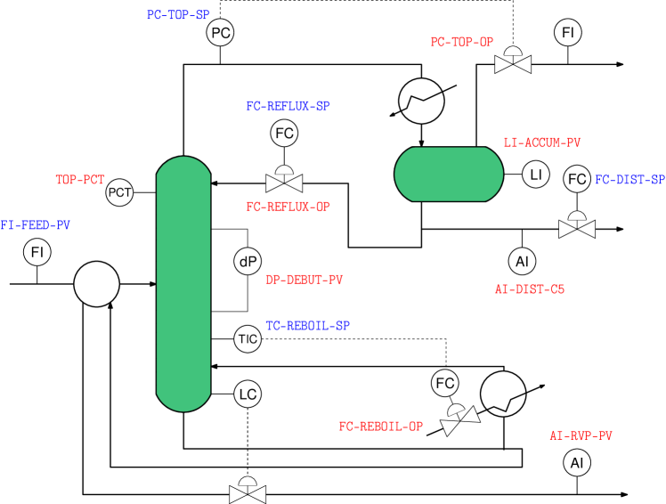
Figure 1: Process flow diagram (PFD) for a debutanizer column, which separates butane and light-end components from a heavier (C5+) hydrocarbon mixture. MVs are highlighted in blue, while CVs are red.

The collinear MV-CV interactions can often be identified based on process data and a priori process knowledge. These interactions may not be exactly collinear in the raw model, but can be corrected by forcing the gain ratios of the collinear MV-CV pairs to be numerically equal. Doing so ensures that the LP will not try to use control handles that are nonexistent.

The near-collinear MV-CV pairs can result in problematic interactions due to numerically ill-conditioned matrices, which, if active, cause undesirable large MV movements to control the near-collinear CVs independently at their constraint limits. In industry, it is common for control practitioners to adjust the steady-state gains manually [2] to deal with ill-conditioning issues. When a gain is changed, its interaction with all of the other gains also changes. Consequently, fixing one gain conditioning issue may create other issues in other parts of the matrix. For further details, Waller and Waller (1995) [3] provides an excellent review of process directionality literature.

An ExxonMobil patent [4] describes a mathematical procedure for adjusting gain matrices. Some commercial applications try to automatically correct the ill-conditioning, such as Honeywell’s RMPCT which uses Singular Value Thresholding (SVT) [5], but automatic techniques can fail because the raw gains can be far enough from the collinearity threshold that they are not fixed. On the other hand, making the SVT threshold large enough to fix these gains could incorrectly remove small but critical interactions/degrees of freedom. Semi-automated techniques, such as those described in a patent by Aspentech [6], may not always produce satisfactory results that are consistent with the process, and may warrant further manual adjustments.

In this paper, we present a novel, non-iterative, binning approach to gain conditioning that significantly reduces the difficulties associated with gain matrix adjustments faced by control practitioners.

II REVIEW OF TECHNIQUES

Two primary tools for analyzing model conditioning are Singular Value Decomposition (SVD), and the Relative Gain Array (RGA).

II-A Singular Value Decomposition

Consider a $2\times 2$ steady-state gain matrix, $G$,

$$G=\bNiceMatrix[first-row,last-col=3]{\footnotesize{\textrm{MV1}}}&{\footnotesize{\textrm{MV2}}}\\ G_{11}G_{12}\footnotesize{\textrm{CV1}}\\ G_{21}G_{22}\footnotesize{\textrm{CV2}}$$ (1)

SVD decomposes $G$ into three matrices with $G=U\Sigma V^{\mathsf{T}}$, describing its most responsive and least responsive directions in terms of both MV moves and CV responses, where

$$\Sigma=\bNiceMatrix\overline{\sigma}&0\\ 0\underline{\sigma}\quad U=\bNiceMatrix[first-row]{\overline{\bm{u}}}&{\underline{\bm{u}}}\\ u_{11}u_{12}\\ u_{21}u_{22}\quad V^{\mathsf{T}}=\bNiceMatrix[last-col]v_{11}^{\mathsf{T}}&v_{12}^{\mathsf{T}}\overline{\bm{v}}^{\mathsf{T}}\\ v_{21}^{\mathsf{T}}v_{22}^{\mathsf{T}}\underline{\bm{v}}^{\mathsf{T}}$$

A physical interpretation of SVD in the context of multivariable control is described in detail by Moore (1986) [7], as illustrated in Fig. 2. CVs will be most responsive in the direction of $\overline{\bm{u}}$ when the MVs are moved in the direction of $\overline{\bm{v}}^{\mathsf{T}}$. The opposite is true for $\underline{\bm{u}}$ and $\underline{\bm{v}}^{\mathsf{T}}$. The singular values $(\overline{\sigma},\underline{\sigma})$ represent the magnitude of each CV direction’s controllability.

Singular values are proportional to system sensitivity [7]; high $\sigma$ values indicate that MV moves will need to be small to maintain accurate control, and vice versa. Singular values that are close to each other indicate that, generally, a controller will be able to control different CVs relatively independently. In contrast, systems with very different singular values will require larger MV moves for disproportionately smaller CV changes. This effect is encapsulated by the condition number, which is defined as the ratio of the largest to the smallest singular value:

$$\gamma={\overline{\sigma}}/{\underline{\sigma}}$$ (2)

It is important to note that the SVD is scale-dependent. The singular values and condition numbers calculated are based on the engineering units of the MVs and CVs.

As an example, consider an unscaled gain matrix in Eq. (3) based on the debutanizer process in Figure 1. MV1 is the TC-REBOILER-SP, MV2 is the FC-REFLUX-SP, CV1 is the AI-RVP-PV in the bottoms and CV2 is the AI-DIST-C5 in the overhead.

$$G=\bNiceMatrix[first-row,last-col=3]{\footnotesize{\textrm{MV1}}}&{\footnotesize{\textrm{MV2}}}\\ -0.1942-0.0029\footnotesize{\textrm{CV1}}\\ 0.1843-0.0288\footnotesize{\textrm{CV2}}$$ (3)

The SVD results based on Eq. (3) are summarized below.

$$U=\begin{bmatrix}[r]-0.7215&0.6925\\ 0.6925&0.7215\end{bmatrix}\quad V=\begin{bmatrix}[r]0.9978&-0.0664\\ -0.0664&-0.9978\end{bmatrix}$$

$$\Sigma=\begin{bmatrix}[c]0.2683&0\\ 0&0.0229\end{bmatrix}$$

The condition number is calculated to be $\gamma=11.74$. However, due to the scale-dependent properties of SVD, the results obtained with Eq. (3) may not be meaningful.

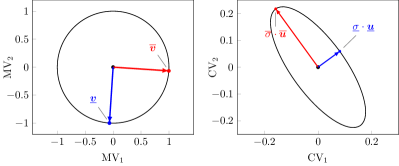
Figure 2: Graphical interpretation of SVD. The left subfigure represents a unit circle of MV input moves, and the right subfigure represents the CV responses. SVD breaks down the CV responses in terms of a ‘strong’ (red) and ‘weak’ (blue) direction illustrated by the CV ellipse. As the weak direction becomes weaker, $\gamma$ increases and the system converges towards collinearity. A collinear matrix would collapse the CV ellipse into a line in the direction of $\overline{\bm{u}}$.

Researchers have proposed various scaling choices, including scaling by physical limits, relative importance of variables, or by other problem-specific scaling that minimizes the condition number to obtain $\gamma_{\min}$ [3]. In practice, a common and useful way to scale the matrix is typical move scaling. This method multiplies each gain by the maximum MV move size made during identification, then divides it by the maximum gain of that CV across all other MVs. The scaled matrix, $G^{\prime}$ using typical move scaling is given by

$$G^{\prime}=S_{b}GS_{a}$$ (4)

where $S_{a}$ and $S_{b}$ are non-zero, diagonal scaling matrices such that $S_{a}=\operatorname{diag}\left(\Delta\textrm{MV}_{1},\Delta\textrm{MV}_{2}\right)$ and $S_{b}=\operatorname{diag}(\underset{i}{\max}(|GS_{a}|)_{1,i},\underset{i}{\max}(|GS_{a}|)_{2,i})^{-1}$. In the first scaling step, the diagonal elements in $S_{a}$ scale each MV column in $G$ by its $\Delta\textrm{MV}$ move size. In the second scaling step, the diagonal elements in $S_{b}$ scale each CV row by dividing each row by that CV’s maximum gain in the $GS_{a}$ matrix.

Typical move scaling ‘normalizes’ the gains by considering both MV move sizes and CV responses to all related MVs. Consequently, small scaled gains may indicate that the gain is small or insignificant, or the MV move size was too small for that CV, or that large MV moves were made with a high-gain CV, making other CV scaled gains look small.

We now consider a scaled gain matrix based on Eq. (3). Let the TC-REBOILER-SP move size, $\Delta\textrm{MV}_{1}=2$, and the FC-REFLUX-SP move size, $\Delta\textrm{MV}_{2}=10$. Using typical move scaling, the gains in each CV now lie between -1 to +1. The scaled gain matrix, $G^{\prime}$ is calculated using Eq. (4) as

$$G^{\prime}=\bNiceMatrix[first-row,last-col=3]{\footnotesize{\textrm{MV1}}}&{\footnotesize{\textrm{MV2}}}\\ -1.0000-0.0754\footnotesize{\textrm{CV1}}\\ 1.0000-0.7813\footnotesize{\textrm{CV2}}$$ (5)

Scaling has changed our understanding of the problem. $\gamma^{\prime}=2.68$ is now smaller for $G^{\prime}$, compared to $\gamma=11.7$ for $G$ prior to scaling. The higher the condition number, the harder it is to drive in the weak direction. From a distillation control perspective, we know that it is much easier to lower the RVP and increase the C5s simultaneously (shift the column composition profile u p), than it is to lower both the RVP and C5s (increase separation) [8].

II-B Relative Gain Array

Inspecting the RGA value is another approach to identify gain ratio issues [9]. The advantage of RGA over SVD is that it is scale independent. In practice, for the gains in a multivariable controller matrix, the RGA is useful in setting an interaction threshold for significant and insignificant gain ratios. For the case of the $2\times 2$ matrix, $G$ in Eq. (1), the RGA computations can be simplified [10] as:

$$\textsc{RGA}=\left(1-\frac{G_{12}\cdot G_{21}}{G_{11}\cdot G_{22}}\right)^{-1}$$ (6)

As the RGA number increases, the gain ratios in the $2\times 2$ matrix approach each other and the matrix approaches singularity. When the gains are collinear, the RGA number is infinite. For an APC model, it is useful to set an RGA threshold such that any gain ratios above a threshold RGA value need to be fixed. For $G$ in Eq. (3), the RGA is calculated to be a desirable, small value of 1.11. In industrial practice, a reasonable 2x2 RGA threshold in a typical multivariable controller could be around 12. Because RGA is independent of scaling, the RGA describes process directionality with regard to inherent process stability, while SVD, because it is considering gain magnitude, does so with regard to performance [8]. From an MPC standpoint, we may or may not be concerned from the performance point of view. Economically we still may want to use the MV with a small directional effect because it costs nothing to do so. For further details and control applications of RGA, the expository text by McAvoy [11] is an excellent resource.

III METHODOLOGY: BINNING THE GAINS

We now present a novel, non-iterative methodology for gain matrix conditioning. The traditional approach involves tedious manual gain adjustments or a complicated optimization analysis that may not converge, until a reasonable RGA value is reached for all submatrices. Our methodology takes a user-defined RGA threshold to generate a discretized grid of $K$ gain values with desirable properties for matrix conditioning.

Given an $N\times M$ gain matrix, there are a total of ${M\choose 2}{\times}{N\choose 2}$ combinations of 2x2 submatrices. By expanding the factorials in the combination terms, it follows that the cost of calculating the RGA for all submatrices is $O(N^{2}M^{2})$. Our method mathematically guarantees that after a single-pass adjustment of all $N\times M$ gains, by matching each gain with the closest ’bin’ in $K$ grid values, all 2x2 submatrices will have an RGA value below the threshold, with a time complexity of $O(NM\cdot\log K)$ using a binary search implementation, without the need to inspect individual submatrices.

Consider any $2\times 2$ non-zero gain matrix, $G$. The gains can be scaled to obtain $K$, such that 3 of the 4 gains are $1$, with a single non-unity gain, $k$, that is dependent on the matrix’s RGA value:

$$K =\begin{bmatrix}[c]1/G_{11}&0\\ 0&1/G_{21}\end{bmatrix}\begin{bmatrix}[c]G_{11}&G_{12}\\ G_{21}&G_{22}\end{bmatrix}\begin{bmatrix}[c]1&0\\ 0&G_{21}/G_{22}\end{bmatrix}$$ (7)

$$=\begin{bmatrix}[c]1&k\\ 1&1\end{bmatrix},\quad\text{where }k=(1-\operatorname{RGA}^{-1})$$

The $k$ term defines the relationship between the gain ratios and the RGA, as shown by rearranging Eq. (6) to get

$$G^{\prime}_{12}/G^{\prime}_{22}=(1-\textsc{RGA}^{-1})\cdot G^{\prime}_{11}/G^{\prime}_{21}$$ (8a)

$$G^{\prime}_{12}/G^{\prime}_{11}=(1-\textsc{RGA}^{-1})\cdot G^{\prime}_{22}/G^{\prime}_{21}$$ (8b)

where Eq. (8a) defines the relationship for the column ratios, and likewise, Eq. (8b) for the rows. For $\operatorname{RGA}=\infty$, $k=1$ and the matrix is singular, meaning that physically, either the MVs or CVs are collinear. For $\operatorname{RGA}=12$, $k=0.9167$. The intuition behind our method is that, instead of just using the matrix gains to compute $k$ and $\operatorname{RGA}$, we could also flip the relationship around to enforce a certain $\operatorname{RGA}$ value for any matrix. This is done by defining our desired $\operatorname{RGA}$, calculating $k$ and then adjusting the gains to equal $k$.

In any typical-move scaled matrix obtained with Eq. (4), the absolute values of the scaled gains lie between $0$ and $1$. Starting with the largest scaled gain of $1$, for $\operatorname{RGA}=12$, the next-largest value is $k=0.9167$ from Eq. (7). To ‘condition’ the matrix, gains between $1$ and $0.9167$ are adjusted to the closest value, either to $1$, enforcing collinearity, or to $0.9167$, enforcing $\operatorname{RGA}=12$.

To cover the entire range of typical move-scaled gains, we now seek a series of values, $k_{1},\cdots,k_{n}$ such that all scaled gains can be adjusted to those values, and the entire matrix can be conditioned to any user-defined RGA threshold. We now ask, what is the next largest value of $k$ that will ensure that the matrix meets the desired $\operatorname{RGA}=12$ threshold? It is found by multiplying $K$ by $k$:

$$K^{(2)} =k\cdot\begin{bmatrix}[c]1&k\\ 1&1\end{bmatrix}=\begin{bmatrix}[c]0.9167&0.8403\\ 0.9167&0.9167\end{bmatrix}$$ (9)

Similar to the first step, the absolute value of the scaled gains between $0.9167$ and $0.8403$ are adjusted to the closest value, either $0.9167$ or $0.8403$. We can repeat this procedure to get $K^{(3)},\cdots,K^{(n)}$ until we generate enough values to cover the range of the scaled gain matrix.

Formally, the pattern in Eq. (9) can be used to construct a recurrence relation that yields a geometric sequence of gains that satisfy a desired RGA threshold. This sequence forms the basis of a set of discretized bins. We define bins as having strictly decreasing bin boundaries, $B_{0},B_{1},\cdots,B_{n}$ such that $B_{i+1}<B_{i}$ for $i={0,1,\cdots,n}$. The bin boundaries define the gain values we can use. The bin width for each interval, $[B_{i+1},B_{i}]$, is given by $w_{i}=B_{i}-B_{i+1}$. This definition constructs $n$ bins with $n+1$ bin boundaries. $n$ is chosen such that the bins cover the range of all gains in the matrix.

Let the first bin boundary be $B_{0}=1$. The next term, $B_{1}$, is found with a recurrence relation derived from Eq. (9) as

$$B_{1}=(1-\textsc{RGA}^{-1})\cdot B_{0}$$

Solving the recurrence relation yields a closed-form solution for any $i$^th bin boundary as a function of $B_{0}$ and RGA:

$$B_{i}=(1-\textsc{RGA}^{-1})^{i}\cdot B_{0}$$ (10)

Consider a scaled gain element $G^{\prime}_{ij}$ in $G^{\prime}$, with an absolute value $|G^{\prime}_{ij}|$ that lies in the interval $B_{k+1}\leq|G^{\prime}_{ij}|<B_{k}$. The binning procedure discretizes $G^{\prime}_{ij}$ to obtain a binned gain, $\widehat{G}_{ij}$, by assigning $G^{\prime}_{ij}$ to the closest boundary with

$$\widehat{G}_{ij}=\operatorname{sgn}{(G^{\prime}_{ij})}\times\begin{cases}B_{k},&\text{if }|G^{\prime}_{ij}|>\frac{B_{k}+B_{k+1}}{2}\\ B_{k+1},&\text{otherwise}\end{cases}$$ (11)

In other words, the procedure simply adjusts the typical-move scaled gain to the closest bin boundary, based on the absolute value of the gain. Due to the exponential term in Eq. (10), the bin widths are also strictly decreasing, such that $w_{k+1}<w_{k}$. It follows that the maximum gain change introduced by this procedure is bounded by the width of the first bin interval $[B_{1},B_{0}]$, with the largest gain adjustment occurring at the midpoint of $[B_{1},B_{0}]$, denoted by $B_{m}$. As shown by the magenta marker in Figure 3, a gain at the midpoint of $[B_{6},B_{5}]$ could be assigned to either boundaries and receive an equal amount of gain adjustment.

Figure 3: Illustration of the binning process. A gain, $g^{\prime}$ that lies in the bin interval $[B_{i+1},B_{i}]$ is adjusted to the closest bin boundary to output a binned gain, $\hat{g}$. Gains that lie on the midpoint of an interval are at equidistant from both bin boundaries, and will experience equal gain adjustment in either direction, as shown by the magenta arrows.

The maximum relative gain change (%), $\delta_{\max}$ is a function of only RGA and independent of the choice of $B_{0}$. By definition, the relative gain change is the ratio of the gain adjustment to the initial gain value, $B_{m}$

$$\delta_{\max}=\frac{B_{0}-B_{m}}{B_{m}}\times 100\%\text{,}\quad B_{m}=\frac{B_{0}+B_{1}}{2}$$ (12)

By substituting Eq. (10) into Eq. (12), the $B_{0}$ terms cancel out and we get $\delta_{\max}=\frac{\operatorname{RGA}^{-1}}{2-\operatorname{RGA}^{-1}}\times 100\%$. The maximum relative gain change percentage as a function of RGA choice is shown in Figure 4. For an RGA choice of 12, the largest relative gain change percentage would have an upper bound of 4.34%, where the 0.9583 midpoint gain is adjusted to either $B_{1}=0.9167$ or to $B_{0}=1.0$.

Figure 4: The maximum relative gain change increases exponentially with smaller RGAs, showing that larger gain adjustments are required to achieve lower RGA values. In practice, for a reasonable RGA threshold of 12, any gain change is guaranteed to at most 4.35%.

The selected RGA threshold builds a binning structure for gains to be fitted into. Note that applying the binning algorithm in a single pass over all gains will honor the RGA threshold for all 2x2 submatrices. Unlike the traditional method, we do not need to inspect individual submatrices and iteratively adjust the entire matrix to maintain the RGA threshold. If new gains are added to the gain matrix at a later time (e.g. controller revamps), they are simply adjusted to the existing binned structure. However, if certain gain values must be preserved (e.g. mass balance constraints), users can choose to adjust only the gains in submatrices that exceed the RGA threshold. All other gains can be left as-is.

The binning procedure is applied to the scaled gain matrix, $G^{\prime}$ in Eq. (5) to obtain binned gains $\widehat{G}$ as shown in Eq. (13). CV1-MV2 was adjusted by 2.5% and CV2-MV2 by 1.4%.

$$\widehat{G}=\bNiceMatrix[first-row,last-col=3]{\footnotesize{\textrm{MV1}}}&{\footnotesize{\textrm{MV2}}}\\ -1.0000-0.07351\footnotesize{\textrm{CV1}}\\ 1.0000-0.77025\footnotesize{\textrm{CV2}}$$ (13)

IV CASE STUDY: DEBUTANIZER PROBLEM

We apply these techniques on the debutanizer process described in Figure 1. Although the operation of a debutanizer seems relatively simple, the process illustrates many complexities commonly faced by APC engineers. The raw gain matrix for the process is shown in Table I with the accompanying debutanizer schematic in Fig. 1.

TABLE I: Original Gains, $G$

	TC-REBOIL-SP	FC-REFLUX-SP	PC-TOP-SP	FC-DIST-SP	FI-FEED-PV
AI-RVP-PV	$-0.1942$	$-0.0029$	$0.0711$	$0$	$0.0013$
AI-DIST-C5	$0.1843$	$-0.0288$	$-0.1907$	$0$	$0.0070$
TOP-PCT	$0.9220$	$-0.1477$	$-0.9458$	$0$	$0.0371$
LI-ACCUM-PV	$0.2042$	$0$	$-0.0667$	$-0.1485$	$0.0381$
DP-DEBUT-PV	$0.0774$	$0.0063$	$-0.0143$	$0$	$0.0064$
PC-TOP-OP	$4.9714$	$0.5000$	$-4.9887$	$0$	$0.3738$
FC-REBOIL-OP	$4.5005$	$0.3391$	$-1.4486$	$0$	$0.2725$
FC-REFLUX-OP	$0$	$0.2651$	$0$	$0$	$0$

The raw gains are scaled according to their typical moves using Eq. (4), and analyzed using SVD and RGA to identify ill-conditioned $2\times 2$ submatrices based on an RGA threshold of 12 and a corresponding condition number of 59, as shown in Table II. The markers indicate that the gain is part of an ill-conditioned $2\times 2$ submatrix based on SVD results (red stars, $\bigstar$), and also on RGA results (blue squares, $\blacksquare$). As shown in Table III, there are 13 pairs above the condition number threshold, and 11 pairs above the RGA threshold. Notice that the first entry with a condition number of 59.1 has a corresponding RGA number of 14.4, while another pair with a condition number of 60 has an RGA number of 10.75. For higher-order sub-matrices, there are 34 $3\times 3$ submatrices of gains with a condition number greater than 100, and 36 $4\times 4$ submatrices with a condition number greater than 100.

TABLE II: Scaled Gains, $G^{\prime}$

	TC-REBOIL-SP	FC-REFLUX-SP	PC-TOP-SP	FC-DIST-SP	FI-FEED-PV
	$\Delta\textrm{MV}=2$	$\Delta\textrm{MV}=10$	$\Delta\textrm{MV}=2$	$\Delta\textrm{MV}=5$	$\Delta\textrm{MV}=10$
AI-RVP-PV	$-1$ $\blacksquare$$\bigstar$	$-0.0754$ $\blacksquare$$\bigstar$	$0.3664$ $\blacksquare$$\bigstar$	$0$ $\blacksquare$$\bigstar$	$0.0337$ $\blacksquare$$\bigstar$
AI-DIST-C5	$0.9666$ $\blacksquare$$\bigstar$	$-0.7552$ $\blacksquare$$\bigstar$	$-1$ $\blacksquare$$\bigstar$	$0$ $\blacksquare$$\bigstar$	$0.1839$ $\blacksquare$$\bigstar$
TOP-PCT	$0.9748$ $\blacksquare$$\bigstar$	$-0.7807$ $\blacksquare$$\bigstar$	$-1$ $\blacksquare$$\bigstar$	$0$ $\blacksquare$$\bigstar$	$0.1962$ $\blacksquare$$\bigstar$
LI-ACCUM-PV	$0.5500$ $\blacksquare$$\bigstar$	$0$ $\blacksquare$$\bigstar$	$-0.1797$ $\blacksquare$$\bigstar$	$-1$ $\blacksquare$$\bigstar$	$0.5129$ $\blacksquare$$\bigstar$
DP-DEBUT-PV	$1$ $\blacksquare$$\bigstar$	$0.4049$ $\blacksquare$$\bigstar$	$-0.1848$ $\blacksquare$$\bigstar$	$0$ $\blacksquare$$\bigstar$	$0.4145$ $\blacksquare$$\bigstar$
PC-TOP-OP	$0.9965$ $\blacksquare$$\bigstar$	$0.5011$ $\blacksquare$$\bigstar$	$-1$ $\blacksquare$$\bigstar$	$0$ $\blacksquare$$\bigstar$	$0.3747$ $\blacksquare$$\bigstar$
FC-REBOIL-OP	$1$ $\blacksquare$$\bigstar$	$0.3767$ $\blacksquare$$\bigstar$	$-0.3219$ $\blacksquare$$\bigstar$	$0$ $\blacksquare$$\bigstar$	$0.3027$ $\blacksquare$$\bigstar$
FC-REFLUX-OP	$0$ $\blacksquare$$\bigstar$	$1$ $\blacksquare$$\bigstar$	$0$ $\blacksquare$$\bigstar$	$0$ $\blacksquare$$\bigstar$	$0$ $\blacksquare$$\bigstar$

TABLE III: Ill-conditioned pairs in $G^{\prime}$

MV1	MV2	CV1	CV2	$\gamma$	RGA
FC-REFLUX-SP	FI-FEED-PV	PC-TOP-OP	FC-REBOIL-OP	59.14	14.36
TC-REBOIL-SP	FI-FEED-PV	DP-DEBUT-PV	PC-TOP-OP	59.99	10.75
TC-REBOIL-SP	PC-TOP-SP	AI-RVP-PV	LI-ACCUM-PV	67.50	9.26
TC-REBOIL-SP	FC-REFLUX-SP	DP-DEBUT-PV	FC-REBOIL-OP	81.83	14.37
FC-REFLUX-SP	PC-TOP-SP	AI-DIST-C5	TOP-PCT	124.38	30.54
TC-REBOIL-SP	PC-TOP-SP	AI-DIST-C5	PC-TOP-OP	131.01	33.24
TC-REBOIL-SP	FC-REFLUX-SP	AI-DIST-C5	TOP-PCT	165.64	40.79
PC-TOP-SP	FI-FEED-PV	AI-DIST-C5	TOP-PCT	169.40	16.04
TC-REBOIL-SP	PC-TOP-SP	TOP-PCT	PC-TOP-OP	181.27	45.81
TC-REBOIL-SP	FI-FEED-PV	AI-DIST-C5	TOP-PCT	189.76	18.39
FC-REFLUX-SP	FI-FEED-PV	AI-DIST-C5	TOP-PCT	276.03	32.66
TC-REBOIL-SP	PC-TOP-SP	AI-DIST-C5	TOP-PCT	472.37	118.54
TC-REBOIL-SP	PC-TOP-SP	LI-ACCUM-PV	FC-REBOIL-OP	530.00	66.23

Applying the binning strategy of Eq. (11) to the scaled gains yields the binned gains in Table IV, which shows each gain’s percentage change in red. The resulting gain matrix has three $2\times 2$ submatrices with an SVD condition number above 59. To eliminate the pairs identified by the condition number threshold, larger gain changes would be required. One of the SVD-identified pairs has an RGA of 8.4. It is therefore unreasonable to remove or adjust the gains associated with this pair because of a somewhat arbitrary SVD condition number. Waller and Waller [3] came to the same conclusion related to using the condition number as a measure of ill-conditioning decades ago.

TABLE IV: Binned Gains, $\widehat{G}$

	TC-REBOIL-SP	FC-REFLUX-SP	PC-TOP-SP	FC-DIST-SP	FI-FEED-PV
AI-RVP-PV	$-1$	$-0.0754$	$0.3664$	$0$	$0.0337$
AI-DIST-C5	$1$ ($3.46\%$)	$-0.7703$ ($2.00\%$)	$-1$	$0$	$0.1914$ ($4.08\%$)
TOP-PCT	$1$ ($2.59\%$)	$-0.7703$ ($-1.34\%$)	$-1$	$0$	$0.1914$ ($-2.41\%$)
LI-ACCUM-PV	$0.5439$ ($-1.11\%$)	$0$	$-0.1755$ ($-2.37\%$)	$-1$	$0.5129$
DP-DEBUT-PV	$1$	$0.4189$ ($3.46\%$)	$-0.1848$	$0$	$0.4189$ ($1.06\%$)
PC-TOP-OP	$1$ ($0.35\%$)	$0.4985$ ($-0.52\%$)	$-1$	$0$	$0.3840$ ($2.49\%$)
FC-REBOIL-OP	$1$	$0.3840$ ($1.93\%$)	$-0.3227$ ($0.25\%$)	$0$	$0.2958$ ($-2.30\%$)
FC-REFLUX-OP	$0$	$1$	$0$	$0$	$0$

Reviewing the matrix, the binned gain matrix has 10 collinear $2\times 2$ pairs, where there were none in the raw matrix. Table V highlights the new collinear pairings.

TABLE V: Collinear Pairs in $\widehat{G}$

Pair	MV1	MV2	CV1	CV2
1	TC-REBOIL-SP	FC-REFLUX-SP	AI-DIST-C5	TOP-PCT
2	TC-REBOIL-SP	PC-TOP-SP	AI-DIST-C5	TOP-PCT
3	TC-REBOIL-SP	FI-FEED-PV	AI-DIST-C5	TOP-PCT
4	FC-REFLUX-SP	PC-TOP-SP	AI-DIST-C5	TOP-PCT
5	FC-REFLUX-SP	FI-FEED-PV	AI-DIST-C5	TOP-PCT
6	PC-TOP-SP	FI-FEED-PV	AI-DIST-C5	TOP-PCT
7	FC-REFLUX-SP	FI-FEED-PV	PC-TOP-OP	FC-REBOIL-OP
8	TC-REBOIL-SP	PC-TOP-SP	LI-ACCUM-PV	FC-REBOIL-OP
9	TC-REBOIL-SP	PC-TOP-SP	AI-DIST-C5	PC-TOP-OP
10	TC-REBOIL-SP	PC-TOP-SP	TOP-PCT	PC-TOP-OP

Notably, the number of $3\times 3$ gain combinations in the binned gain matrix above a condition number of 100 has been reduced from 34 in the raw matrix to two. The condition numbers of the two $3\times 3$ matrices are 135 and 105. Similarly, the number of $4\times 4$ gain combinations with a higher condition number than 100 has been reduced from 36 to 1, where that condition number is 156. By conditioning the $2\times 2$ gains, the conditioning of the entire gain matrix has improved significantly. It is important to note that a high condition number on a higher-order matrix does not necessarily mean that this combination of gains will be active in an LP solution. Still, reducing the high condition number interactions means that it is impossible for such combinations to play a part in the LP solution under any situation.

V DISCUSSIONS

How do we know if a gain pair should be collinear or not collinear? Often the answer relies on process knowledge. Second to process understanding, if a gain pair is nearly collinear, removing the degree of freedom based on a high RGA or condition number is reasonable.

In the debutanizer example, the TOP-PCT is a pressure compensated temperature, and it should be collinear with the AI-DIST-C5 composition. In the binned matrix, it is collinear since the scaled gains are equal. However, if one or more of the gains had been slightly bigger or smaller, the binning process would put the gain in a bin above or below the correct bin. If this were to happen, a degree of freedom would exist in the model where none should be. The opposite situation is also possible, where a degree of freedom is removed in a set of gains where one should exist.

Under certain circumstances, ill-conditioned gains may not be a problem in the controller. Why would we even include the TOP-PCT in the model if we have AI-DIST-C5 which serves the same purpose of measuring C5 composition? One reason is the C5 analyzer may not be reliable. If the controller is intermittently hitting the AI-DIST-C5 or TOP-PCT upper limit, with an unconditioned gain matrix, the LP may believe that temporarily it can control both CVs. As long as the CV limits are spread widely, and the gains are nearly collinear, there likely will be no observed problems. The RGA number is high, but the LP is not trading off the degrees of freedom that exist between the two CVs.

Conditioning problems for this case become apparent when the analyzer starts to drift, and the controller tries to control one CV at a high limit, and the other at a low limit. A properly conditioned model will have no difference in the gain ratios of the two CVs, and when the LP is faced with conflicting limits, it will simply give up on the least important CV. An unconditioned model will find small degrees of freedom that will allow the LP to trade off MV moves that try to fix the problem. If the CV gain ratios are a little farther from collinearity, the moves to control CVs at different limits may not be large, but the LP will drive the process in unreasonable directions and CV errors will not be reduced. When differences in gain ratios of collinear variables exist, the controller LP may find a different solution based on which CV limit is active. This can lead to optimization cost tuning in order to get the controller to behave the same way when faced with high or low limits on either variable.

The gain issues described can spread to higher dimensions as well, and the issues are often magnified when the optimizer becomes infeasible. As long as the MV directions that try to solve the infeasibility are the same as the feasible economic direction, little changes may be noticed when the solution becomes infeasible. When the infeasible direction opposes the economic direction, the controller can make large moves in an uneconomic direction trying to reduce or eliminate CV error. From these behaviors, the practitioner may erroneously conclude that the model is inaccurate and needs re-evaluation. A “good” but unconditioned model can account for this behavior. Retesting to fix an ill-conditioned matrix is unlikely to solve the problem.

These simple examples show why binning the gains is not the final answer, rather the first step in the overall model gain analysis. The “correct” structure of the gain matrix must be determined based on plant data and process understanding. The binning procedure makes the next step of validating the model gain structure much easier. In a real-world MPC project, the practitioner must perform an interaction analysis of the model gains by simulating the LP solution.

VI CONCLUSIONS

In this paper, we have demonstrated a binning procedure to condition the gain matrix used in industrial MPCs. By conditioning the matrix, we remove small degrees of freedom that are either insignificant or zero, without large perturbations to the process gains. This gain conditioning step prevents the optimizer from erroneously exploiting small degrees of freedom for control. The binning approach can also include small gains in the model to maintain gain consistency and respect material balances, without introducing further conditioning problems.

There are several areas of interesting future work here. The tables presented earlier for identifying gain interactions using markers are quite basic - as these tables grow in size, this colour-based strategy can result in cluttered and unintuitive displays, making near-collinearity analysis visually difficult. There is an opportunity for improving the visualization of degrees of freedom and gain ratios. We have made some recent progress in visualizing the LP solution for troubleshooting and understanding online MPCs [12].

Unlike SVD, higher-order RGA calculations rely on the matrix inverse, which does not exist for a rank-deficient matrix with collinearities. Therefore, to identify conditioning issues in larger submatrices, the RGA is mathematically undefined and cannot be used, and SVD may not be entirely reliable either due to scaling issues. In industry, higher-dimensional analysis of the gain matrix beyond $3\times 3$ submatrices are often not investigated by practitioners. It may be that a higher order RGA analysis could be useful once all $2\times 2$ submatrices have been conditioned to the desired RGA threshold. The goal, in practice, has always been to certify that a model is conditioned to the dimensionality of the problem. Here the dimensionality is defined as a square case, corresponding to the lesser of the number of MVs or the number CVs. For a non-square SVD case, the extra variables generally guarantee that there are significant directions related to the degrees of freedom in the matrix. With SVD, it seems reasonable that for a specific problem, we should be able to identify physically meaningful orthogonal directions in the model, and then force the model gains to follow combinations of these directions.

References

- [1] J. M. Maciejowski, Predictive Control: With Constraints. Prentice Hall, 2002.
- [2] A. Ishikawa, M. Ohshima, and M. Tanigaki, “A practical method of removing ill-conditioning in industrial constrained predictive control,” Computers & Chemical Engineering, May 1997.
- [3] J. B. Waller and K. V. Waller, “Defining directionality: Use of directionality measures with respect to scaling,” Industrial & engineering chemistry research, vol. 34, no. 4, pp. 1244–1252, 1995.
- [4] R. S. Hall, T. J. Peterson, T. S. Pottorf, A. R. Punuru, and L. E. Vowell, “Method for model gain matrix modification,” CA Patent CA2 661 478A1, Feb., 2008.
- [5] S. J. Qin and T. A. Badgwell, “A survey of industrial model predictive control technology,” Control engineering practice, vol. 11, no. 7, pp. 733–764, 2003.
- [6] Q. Zheng, M. J. Harmse, K. H. Rasmussen, and B. Mcintyre, “Methods and articles for detecting, verifying, and repairing matrix collinearity,” CA Patent CA2 519 783C, Mar., 2014.
- [7] C. Moore, “Application of Singular Value Decomposition to the Design, Analysis, and Control of Industrial Processes,” in 1986 American Control Conference, June 1986, pp. 643–650.
- [8] M. F. Sgfors and K. V. Waller, “Multivariable control of ill-conditioned distillation columns utilizing process knowledge,” Journal of Process Control, vol. 8, no. 3, pp. 197–208, 1998.
- [9] E. Bristol, “On a new measure of interaction for multivariable process control,” IEEE transactions on automatic control, vol. 11, no. 1, pp. 133–134, 1966.
- [10] A. Brambilla and L. D’Elia, “Multivariable controller for distillation columns in the presence of strong directionality and model errors,” Industrial & engineering chemistry research, vol. 31, no. 2, pp. 536–543, 1992.
- [11] T. J. McAvoy, Interaction Analysis: Principles and Applications. Instrument Society of America, 1983, vol. 6.
- [12] S. Elnawawi, L. C. Siang, D. L. O’Connor, and R. B. Gopaluni, “Interactive visualization for diagnosis of industrial Model Predictive Controllers with steady-state optimizers,” Control Engineering Practice, vol. 121, p. 105056, Apr. 2022.