Insights into the equation of state of neutron-rich matter since GW170817

Abstract

The historical detection of gravitational waves emitted from the binary neutron star merger GW170817 has opened the new era of multi-messenger astronomy. Since then, many other significant discoveries—both on heaven and earth—are providing new clues into the behavior of neutron-rich matter. It is the goal of this article to illustrate how the remarkable progress made during the last few years is spearheading the field into the golden age of neutron-star physics [1].

1 Introduction

The last five years have provided a plethora of exciting new discoveries that have dramatically advanced our quest to answer some of the most fundamental questions stimulating nuclear science today. Among the eleven science questions for the next century identified by the National Academies Committee on the Physics of the Universe [2], two of them are particularly relevant to nuclear science: (i) What are the new states of matter at exceedingly high density and temperature? and (ii) how were the elements from iron to uranium made?

In one clean sweep, the first direct detection of gravitational waves emitted from the binary neutron star merger GW170817 is providing critical insights into the nature of dense matter and on the creation of the heavy elements in the cosmos [3]. Indeed, just a few hours after the gravitational-wave detection, ground- and spaced-based telescopes identified the associated kilonova—the electromagnetic transient assumed to be powered by the radioactive decay of the heavy elements synthesized in the rapid neutron-capture process ($r$-process). The observed light curve appears consistent with the large opacity of the lanthanides ($Z\!=\!57\!-\!71$) [4, 5, 6, 7]. Although highly suggestive, at present there is no firm evidence that the heavier actinides were also created by GW170817.

In the context of the equation of state (EOS) the main contribution from GW170817 was the extraction of the tidal deformability—or tidal polarizability—a property that is encoded in the gravitational-wave profile. The tidal polarizability is an intrinsic neutron-star property that is highly sensitive to the compactness parameter [8, 9, 10, 11, 12, 13]. The dimensionless tidal polarizability is given by

$$\Lambda=\frac{2}{3}k_{2}\left(\frac{c^{2}R}{GM}\right)^{5}=\frac{64}{3}k_{2}\left(\frac{R}{R_{s}}\right)^{5}\;,$$ (1)

where $k_{2}$ is the second Love number [14, 15], $M$ and $R$ are the neutron star mass and radius, respectively, and $R_{s}\!\equiv\!2GM/c^{2}$ is the Schwarzschild radius of the star. A great virtue of the tidal polarizability is its sensitivity to the stellar radius ($\Lambda\!\!\sim\!\!R^{5}$) a quantity that has been notoriously difficult to constrain through electromagnetic obervations [16, 17, 18, 19, 20]. The tidal polarizability describes the tendency of a neutron star to develop a mass quadrupole in response to the tidal field generated by its companion [21, 22]. In the linear regime, the induced quadrupole moment is proportional to the tidal field, with the constant of proportionality being the tidal polarizability.

Figure 1: The nuclear equation of state ladder. Akin to the cosmic distance ladder in cosmology, the equation of state ladder represents a succession of both experimental and observational methods to determine how the pressure changes with increasing density. Given that the range of densities spanned in a neutron star is enormous, no single method can determined the entire EOS. Each rung of the ladder provides information that can be used to determine the EOS at the next higher or lower rung.

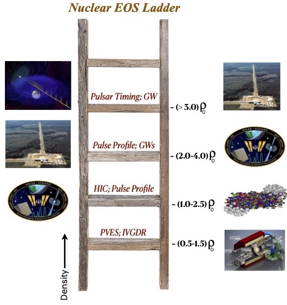
However, since the detection of GW170817 many other significant discoveries have been made which have further strengthen the synergy between Nuclear Physics and Astrophysics. Principal among these are the detection of the heaviest neutron star to date [23], the first ever simultaneous determination of the mass and radius of a neutron star [24, 25], and the largely model-independent extraction of the neutron skin thickness of ²⁰⁸Pb [26]. All these discoveries motivate the creation of an “EOS ladder” akin to what is known in cosmology as the cosmic distance ladder; see Fig.1. Each rung in the ladder represents an experimental/observational technique that constraints the EOS at progressively higher or lower densities. The first rung in the ladder consists of laboratory experiments that constrain the EOS in the vicinity of nuclear saturation density. The next rungs include both electromagnetic observations and gravitational wave detections that constrain the EOS at about two-to-four times saturation density. Finally, the highest rung in the ladder involves observations of the most massive neutron stars, which constrain the EOS at the highest densities found in the stellar core.

2 Pulsar Timing: Weighing Neutron Stars

According to Newton’s law of universal gravitation, all that can be determined from the orbiting motion of two stellar objects is their combined mass. Indeed, according to Kepler’s third law of planetary motion, the orbiting period of the binary system around their common center of mass is given by:

$$P^{2}=\frac{4\pi^{2}}{G(M_{1}+M_{2})}a^{3},$$ (2)

where $P$ is the orbital period, $a$ is the length of the semi-major axis, and $M_{1}$ and $M_{2}$ are the individual masses of the two orbiting bodies. To break the degeneracy and determine the individual masses one most invoke general relativity.

Figure 2: Regarded as the “fourth” test of general relativity, the Shapiro delay may be used to infer the mass of the companion star, thereby breaking the degeneracy present in Newtonian gravity. (a) An artist rendition of Shapiro delay as the electromagnetic radiation emitted from the neutron star is bended by the gravitational field from the companion. (b) Timing residual (in micro-seconds) for the binary system consisting of the pulsar J1614-2230 and its white-dwarf companion. Adapted from Ref.[27].

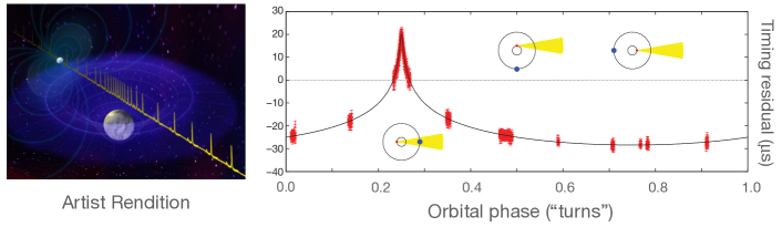
The Shapiro delay [28] is a powerful technique that has been used effectively to measure some of the most massive neutron stars to date [23, 27, 29]. The main notion behind the Shapiro delay is that even massless particles such as photons bend due to the curvature of space-time around a massive object. This will cause a time delay in the arrival of the electromagnetic radiation emitted by the neutron star on its way to the observer as it “dips” into the gravitational potential of the companion. Thus, pulsar timing—an observational strategy that is able to account for every rotation of the neutron star and hence monitor its time structure over long periods of time—can provide highly accurate values for the masses of both the neutron star and its companion. Figure 2 shows an artist rendition of the Shapiro delay as the electromagnetic radiation emitted by the neutron star is bended by the space-time distortion induced by the companion. The figure also shows the timing residuals over one complete orbital period of the pulsar J1614-2230 in orbit with a white-dwarf star observed by the Green Bank Telescope [27]. Extracting the mass of the companion white-dwarf star from the Shapiro delay, combined with Kepler’s third law, allows one to break the Newtonian degeneracy and determine the mass of both stars. In particular, the mass of the neutron star was found to be $M\!=\!1.97\pm 0.04\,M_{\odot}$. More recently, the Shapiro delay was used to reveal the mass of the millisecond pulsar J0740+6620, that with a mass of $M\!=\!2.1^{+0.10}_{-0.09}\,M_{\odot}$ represents the most massive (well measured) neutron star to date [23]; note that this value was later refined to $M\!=\!2.08\!\pm\!0.07\,M_{\odot}$ [29].

3 Pulsar Profile: Sizing Neutron Stars

Just like white-dwarf stars, neutron stars collapse after they reach a maximum mass. However, unlike white-dwarf stars, the radius of the maximum mass configuration remains finite. Beyond such limiting mass, neutron stars collapse because the hydrostatic configuration becomes unstable against small density perturbations. The determination of the (presently unknown) limiting mass provides a powerful constraint on the high-density component of the equation of state. However, the determination of the entire EOS requires knowledge of the stellar radius as a function of mass. Although it is well known that a given EOS generates a unique mass-radius (MR) profile, the fact that the opposite is also true is not as widely known. That is, knowledge of the MR relation also uniquely determines the underlying neutron-star matter equation of state [30, 31].

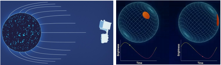
Until very recently, no single neutron star had both their mass and radius simultaneously determined. This changed recently with the deployment of the Neutron Star Interior Composition Explorer (NICER) aboard the international space station. The main idea behind measuring stellar radii with NICER, or more appropriately the stellar compactness, is the identification and monitoring of “hot spots” on the stellar surface. Magnetic fields in pulsars are so strong and complex that charged particles that are ripped away from the star often crash back into the stellar surface creating hot spots, namely, regions within the star that glow brighter than the rest of the star. As the neutron star spins, the hot spots come in and out of view producing periodic variations in the brightness—or pulse profile—that are recorded by NICER. And just as the Shapiro delay takes advantage of general relativistic effects, so does NICER. Indeed, the gravitational field around the neutron star is so strong, that x-rays emitted from the back of the star get bent and are eventually detected by NICER’s sophisticated instruments. For a highly compact neutron star, the hot spots never disappear: NICER actually sees the back of the star!

So far NICER has determined the mass and radius of two neutron stars. The first mass-radius determination was for the millisecond pulsar PSR J0030+0451. The two independent—and fully consistent—determinations yielded:

$$M=1.34^{+0.15}_{-0.16}\,M_{\odot}\hskip 5.0pt{\rm and}\hskip 5.0ptR=12.71^{+1.14}_{-1.19}\,{\rm km}\;\cite[cite]{[\@@bibref{}{Riley:2019yda}{}{}]},$$ (3a)

$$M=1.44^{+0.15}_{-0.14}\,M_{\odot}\hskip 5.0pt{\rm and}\hskip 5.0ptR=13.02^{+1.24}_{-1.06}\,{\rm km}\;\cite[cite]{[\@@bibref{}{Miller:2019cac}{}{}]}.$$ (3b)

Although pioneering, the precision of the first NICER measurement was hindered by the absence of an independent determinationt of the mass of J0030+0451.

Figure 3: NICER relies on one of the most dramatic consequences of general relativity: the bending of light. The left-hand panel illustrates how the strong gravitational field created by a neutron star bends x-rays emitted from the back of the star that are then collected by NICER. The right-hand panel shows how these x-rays emitted from a hot spot may be detected with an unprecedented time resolution that allows for the accurate reconstruction of the pulse profile.

The second mass-radius determination was for the millisecond pulsar PSR J0740+6620, the very same heaviest neutron star whose mass was independently determined using Shapiro delay [23, 29]. For this neutron star, the reported mass and radius are given by [32]

$$M=2.072^{+0.067}_{-0.066}\,M_{\odot}\hskip 5.0pt{\rm and}\hskip 5.0ptR=12.39^{+1.30}_{-0.98}\,{\rm km},$$ (4)

in complete agreement with the mass obtained using Shapiro delay [29]. Moreover, when both NICER measurements are combined with other high-mass constraints, as well as with the tidal deformability extracted from GW170817, the radius of a canonical $1.4\,M_{\odot}$ neutron star and of a $2.08\,M_{\odot}$ neutron star were determined with unprecedented precision [33]:

$$R=12.45\pm 0.65\,{\rm km}\hskip 5.0pt{\rm for}\hskip 5.0ptM=1.40\,M_{\odot},$$ (5a)

$$R=12.35\pm 0.75\,{\rm km}\hskip 5.0pt{\rm for}\hskip 5.0ptM=2.08\,M_{\odot}.$$ (5b)

This is truly a remarkable result, as it suggests that the equation of state at the highest densities ever probed is not soft. Moreover, it justifies an earlier conjecture that suggests that neutron stars share a common radius over a wide mass range [19].

4 Electron Scattering: Sizing Atomic Nuclei

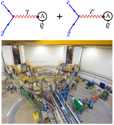
For more than six decades, elastic electron scattering has painted the most compelling picture of the distribution of electric charge in an atomic nucleus [34]. The charge distribution, carried primarily by the protons, has been mapped with remarkable precision throughout the nuclear chart [35, 36]. In contrast, neutron densities are largely determined using hadronic experiments that are hindered by large and uncontrolled uncertainties [37]. The Lead Radius EXperiment (PREX) improved dramatically this situation by also using elastic electron scattering to map the neutron distribution. Although neutrons do not carry electric charge, they do carry a weak charge that couples to the neutral weak vector boson $Z^{0}$. Given that the weak interaction violates parity, an asymmetry emerges from a quantum mechanical interference of two Feynman diagrams: a large one involving the exchange of a photon and a much smaller one involving the exchange of a $Z^{0}$ boson, as in Fig. 4.

Figure 4: Parity violating elastic electron scattering is a clean, largely model independent technique to determine the neutron distribution of atomic nuclei. The parity violating asymmetry develops from the interference of two Feynman diagrams. PREX has pioneered and perfected this challenging technique that produces asymmetries of only about one part in a million, and relies on the five-story high spectrometer located at the Thomas Jefferson National Accelerator Facility. PREX has provided an estimate for the neutron skin thickness of ²⁰⁸Pb: $R_{\rm skin}\!=\!(0.283\pm 0.071)\,{\rm fm}$ [26].

The parity-violating asymmetry is defined as

$$A_{PV}(Q^{2})=\frac{\displaystyle{\left(\frac{d\sigma}{d\Omega}\right)_{\!\!R}-\left(\frac{d\sigma}{d\Omega}\right)_{\!\!L}}}{\displaystyle{\left(\frac{d\sigma}{d\Omega}\right)_{\!\!R}+\left(\frac{d\sigma}{d\Omega}\right)_{\!\!L}}}\xrightarrow[\text{}]{\text{P.W.}}\frac{G_{\!F}Q^{2}}{4\pi\alpha\sqrt{2}}\frac{Q_{\rm wk}F_{\rm wk}(Q^{2})}{ZF_{\rm ch}(Q^{2})},$$ (6)

where $(d\sigma\!/d\Omega)_{R/L}$ is the differential cross section for the elastic scattering of right/left-handed longitudinally polarized electrons, and the arrow indicates that a plane-wave approximation that ignores Coulomb distortions has been adopted [38, 39, 40]. The right-hand side of the expression depends on the four-momentum transfer $Q^{2}$, the fine structure $\alpha$ and Fermi $G_{\!F}$ constants, and the electric $Z$ and weak $Q_{\rm wk}$ nuclear charges. As such, all nuclear-structure information is contained in the ratio between the weak and the charge form factors, both of them normalized to one at $Q^{2}\!=\!0$. Note that the form factors are related to the corresponding spatial distributions by a Fourier transform. Given that the charge form factor for ²⁰⁸Pb is accurately known [41], the parity violating asymmetry provides vital—and model-independent—information on the weak form factor, which is dominated by the neutrons [42]. PREX has provided the first model-independent evidence that the rms radius of the neutron distribution in ²⁰⁸Pb is larger than the corresponding radius of the proton distribution. The difference between these two radii is known as the neutron skin thickness, a dilute region of the nucleus populated primarily by neutrons. Notably, the neutron skin thickness of ²⁰⁸Pb is strongly correlated to a fundamental parameter of the equation of state: the pressure of pure neutron matter at saturation density [40, 43, 44, 45]. Thus PREX provides a unique portal to the equation of state and forms the first rung of the EOS ladder depicted in Fig.1. By combining an early experiment [46, 47] with the most recent one [26], PREX has delivered on its promise to determine the neutron radius of ²⁰⁸Pb with a precision of nearly 1%, which in turn results in a neutron skin thickness of

$$R_{\rm skin}\equiv R_{n}-R_{p}=(0.283\pm 0.071)\,{\rm fm}.$$ (7)

5 Insights into the EOS since GW170817

So what have we learned about the equation of state of neutron rich matter since GW170817. We summarize the main findings in Fig. 5. The left-hand panel displays combined constraints from the tidal deformability and radius of a $1.4\,M_{\odot}$ neutron star obtained from LIGO and NICER, respectively, and from the neutron skin thickness of ²⁰⁸Pb extracted by the PREX collaboration. Also shown with the individual circles are predictions for all three observables by a collection of accurately calibrated energy density functionals. It is important to underscore that after calibration, each individual functional predicts all these observables without any further fine tuning of parameters. That is, the aim of each individual model is to predict within a single theoretical framework both the properties of finite nuclei and the structure of neutron stars [48].

Figure 5: The left-hand graph displays the tidal polarizability of a $1.4M_{\odot}$ neutron star as a function of both its radius and the neutron skin thickness of ${}^{208}{\rm Pb}$. The circles denote the predictions from several accurately calibrated covariant energy density functionals. The rectangular sections delineate the regions that are consistent with the various experiments/observations. The right-hand graph shows the mass-radius relation as predicted by a subset of the models. Also shown are constraints obtained from theory, electromagnetic observations, and gravitational-wave detections, as articulated in the text.

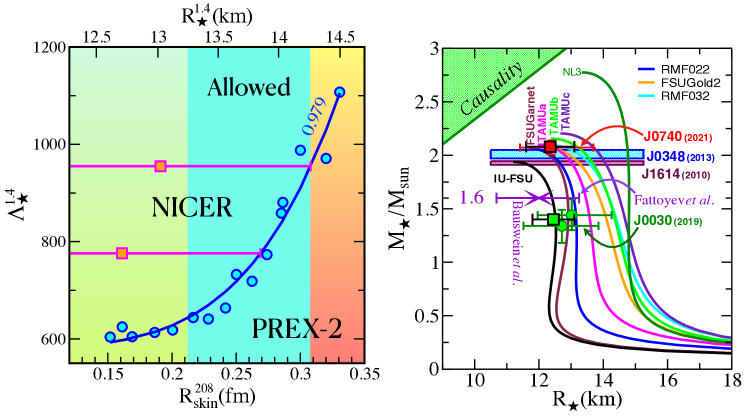
Given the strong correlation between all three observables, one can now search for models that satisfy all the constraints. In particular, the strong correlation observed in our models between $R_{\star}^{1.4}$ – $R_{\rm skin}$ provides an upper limit on the neutron skin thickness of $R_{\rm skin}\!\lesssim\!0.31\,{\rm fm}$ and a lower limit on the stellar radius of $R_{\star}^{1.4}\!\gtrsim\!13.25\,{\rm km}$. The region that satisfies both the PREX and NICER constraints is indicated by the narrow (blue) rectangle in the middle of the figure, which excludes models with either a very stiff or a very soft EOS. Note that a stiff(soft) EOS is one in which the pressure increases rapidly(slowly) with density. Moreover, given that the tidal deformability scales with the fifth power of the stellar radius [49], one can also set limits on the tidal deformability of a $1.4\,M_{\odot}$ neutron star. Combining all these results one obtains [50]:

$$0.21\lesssim \;R_{\rm skin}({\rm fm})\!\lesssim 0.31$$ (8a)

$$13.25\lesssim \;R_{\star}^{1.4}({\rm km})\!\lesssim 14.26$$ (8b)

$$642\lesssim \;\Lambda_{\star}^{1.4}\!\lesssim 955.$$ (8c)

The allowed region for the tidal deformability is consistent with the $\Lambda_{\star}^{1.4}\!\lesssim\!800$ limit reported in the GW170817 discovery paper [3], yet it is outside the $\Lambda_{1.4}\!\lesssim\!580$ limit suggested in the revised paper [51]. If confirmed, this will create some serious tension—at least relative to the models presented here—and may suggest the onset of a phase transition. Indeed, the PREX result suggests that the equation of state is stiff in the vicinity of nuclear saturation density. However, the EOS will have to soften considerably at intermediate densities to accommodate the revised limit on $\Lambda_{\star}^{1.4}$. Ultimately, however, the EOS will need to stiffen at the highest densities to account for the existence of $\sim\!2\,\!M_{\odot}$ neutron stars.

Finally, we display on the right-hand side of Fig. 5 the “holy grail” of neutron-star structure: the mass-radius relation. The theoretical predictions are made by a subset of models used on the left-hand panel. Also incorporated into the plot are several of the high-quality astronomical data that have been collected since GW170817. By incorporating both gravitational-wave and electromagnetic information from GW170817, Bauswein and collaborators were able to provide a lower limit on the radius of a $1.6M_{\odot}$ neutron star [52]. By combining this analysis with the upper limits obtained in Refs. [49, 53], one obtains the two arrows facing each other in the figure, suggesting that the stellar radius of a $1.6M_{\odot}$ neutron star must fall in the 10.6-13.3 km interval. Also shown in the figure are simultaneous mass and radius determinations of the two millisecond pulsars J0030+0451 and J0740+6620. However, what is most impressive is the fairly precise radii for a $1.4\,M_{\odot}$ and a $2.08\,M_{\odot}$ neutron stars [33] inferred by combining LIGO and NICER data with previous determinations of the other two $\sim\!2\,M_{\odot}$ neutron stars: J1614 [27] and J0348 [54]. These two inferences are displayed in the figure by the two squares and show their dramatic impact on the MR relation, and ultimately on the equation of state. Remarkably, before GW170817 all the astronomical data that would have appeared in the figure are the two mass measurements for J1614 and J0348 and nothing else. The progress since GW170817 has been tranformational, marking the arrival of the golden age of neutron-star physics [1].

References

- [1] Baym G 2019 JPS Conf. Proc. 26 011001
- [2] 2003 Connecting Quarks with the Cosmos: Eleven Science Questions for the New Century (Washington: The National Academies Press)
- [3] Abbott B P et al. (Virgo, LIGO Scientific) 2017 Phys. Rev. Lett. 119 161101
- [4] Drout M R et al. 2017 Science 358 1570–1574
- [5] Cowperthwaite P S et al. 2017 Astrophys. J. 848 L17
- [6] Chornock R et al. 2017 Astrophys. J. 848 L19
- [7] Nicholl M et al. 2017 Astrophys. J. 848 L18
- [8] Hinderer T 2008 Astrophys. J. 677 1216–1220
- [9] Hinderer T, Lackey B D, Lang R N and Read J S 2010 Phys. Rev. D81 123016
- [10] Damour T and Nagar A 2009 Phys. Rev. D80 084035
- [11] Postnikov S, Prakash M and Lattimer J M 2010 Phys. Rev. D82 024016
- [12] Fattoyev F J, Carvajal J, Newton W G and Li B A 2013 Phys. Rev. C87 015806
- [13] Steiner A W, Gandolfi S, Fattoyev F J and Newton W G 2015 Phys. Rev. C91 015804
- [14] Binnington T and Poisson E 2009 Phys. Rev. D80 084018
- [15] Damour T, Nagar A and Villain L 2012 Phys. Rev. D85 123007
- [16] Ozel F, Baym G and Guver T 2010 Phys. Rev. D82 101301
- [17] Steiner A W, Lattimer J M and Brown E F 2010 Astrophys. J. 722 33
- [18] Suleimanov V, Poutanen J, Revnivtsev M and Werner K 2011 Astrophys. J. 742 122
- [19] Guillot S, Servillat M, Webb N A and Rutledge R E 2013 Astrophys. J. 772 7
- [20] Nattila J, Miller M C, Steiner A W, Kajava J J E, Suleimanov V F and Poutanen J 2017 Astron. Astrophys. 608 A31
- [21] Damour T, Soffel M and Xu C M 1992 Phys. Rev. D45 1017–1044
- [22] Flanagan E E and Hinderer T 2008 Phys. Rev. D77 021502
- [23] Cromartie H T et al. 2019 Nat. Astron. 4 72–76
- [24] Riley T E et al. 2019 Astrophys. J. Lett. 887 L21
- [25] Miller M C et al. 2019 Astrophys. J. Lett. 887 L24
- [26] Adhikari D et al. (PREX) 2021 Phys. Rev. Lett. 126 172502
- [27] Demorest P, Pennucci T, Ransom S, Roberts M and Hessels J 2010 Nature 467 1081
- [28] Shapiro I I 1964 Phys. Rev. Lett. 13 789
- [29] Fonseca E et al. 2021 Astrophys. J. Lett. 915 L12
- [30] Lindblom L 1992 Astrophys. J. 398 569
- [31] Chen W C and Piekarewicz J 2015 Phys. Rev. Lett. 115 161101
- [32] Riley T E et al. 2021 Astrophys. J. Lett. 918 L27
- [33] Miller M C et al. 2021 Astrophys. J. Lett. 918 L28
- [34] Hofstadter R 1956 Rev. Mod. Phys. 28 214–254
- [35] Fricke G, Bernhardt C, Heilig K, Schaller L A, Schellenberg L, Shera E B and de Jager C W 1995 Atom. Data and Nucl. Data Tables 60 177
- [36] Angeli I and Marinova K 2013 At. Data Nucl. Data Tables 99 69 – 95
- [37] Thiel M, Sfienti C, Piekarewicz J, Horowitz C J and Vanderhaeghen M 2019 J. Phys. G46 093003
- [38] Horowitz C J 1998 Phys. Rev. C57 3430–3436
- [39] Roca-Maza X, Centelles M, Salvat F and Vinas X 2008 Phys. Rev. C78 044332
- [40] Roca-Maza X, Centelles M, Viñas X and Warda M 2011 Phys. Rev. Lett. 106 252501
- [41] De Vries H, De Jager C W and De Vries C 1987 Atom. Data Nucl. Data Tabl. 36 495–536
- [42] Donnelly T, Dubach J and Sick I 1989 Nucl. Phys. A503 589
- [43] Brown B A 2000 Phys. Rev. Lett. 85 5296
- [44] Furnstahl R J 2002 Nucl. Phys. A706 85–110
- [45] Centelles M, Roca-Maza X, Viñas X and Warda M 2009 Phys. Rev. Lett. 102 122502
- [46] Abrahamyan S, Ahmed Z, Albataineh H, Aniol K, Armstrong D S et al. 2012 Phys. Rev. Lett. 108 112502
- [47] Horowitz C J, Ahmed Z, Jen C M, Rakhman A, Souder P A et al. 2012 Phys. Rev. C85 032501
- [48] Yang J and Piekarewicz J 2020 Ann. Rev. Nucl. Part. Sci. 70 21–41
- [49] Fattoyev F J, Piekarewicz J and Horowitz C J 2018 Phys. Rev. Lett. 120 172702
- [50] Reed B T, Fattoyev F J, Horowitz C J and Piekarewicz J 2021 Phys. Rev. Lett. 126 172503
- [51] Abbott B P et al. (Virgo, LIGO Scientific) 2018 Phys. Rev. Lett. 121 161101
- [52] Bauswein A, Just O, Janka H T and Stergioulas N 2017 Astrophys. J. 850 L34
- [53] Annala E, Gorda T, Kurkela A and Vuorinen A 2018 Phys. Rev. Lett. 120 172703
- [54] Antoniadis J, Freire P C, Wex N, Tauris T M, Lynch R S et al. 2013 Science 340 6131