Extraction of $\alpha_{s}$ using Borel-Laplace sum rules for tau decay data

Abstract

Double-pinched Borel-Laplace sum rules are applied to ALEPH $\tau$-decay data. For the leading-twist ($D=0$) Adler function a renormalon-motivated extension is used, and the 5-loop coefficient is taken to be $d_{4}=275\pm 63$. Two $D=6$ terms appear in the truncated OPE ($D\leq 6$) to enable cancellation of the corresponding renormalon ambiguities. Two variants of the fixed order perturbation theory, and the inverse Borel transform, are applied to the evaluation of the $D=0$ contribution. Truncation index $N_{t}$ is fixed by the requirement of local insensitivity of the momenta $a^{(2,0)}$ and $a^{(2,1)}$ under variation of $N_{t}$. The averaged value of the coupling obtained is $\alpha_{s}(m_{\tau}^{2})=0.3235^{+0.0138}_{-0.0126}$ [$\alpha_{s}(M_{Z}^{2})=0.1191\pm 0.0016$]. The theoretical uncertainties are significantly larger than the experimental ones.

The sum rule corresponding to the application of the Cauchy theorem to a contour integral containing the ($u$-$d$) quark $V+A$ correlator $\Pi(Q^{2})$ ($Q^{2}\equiv-q^{2}$) and a weight function $g(Q^{2})$, $\oint_{C_{1}+C_{2}}dQ^{2}g(Q^{2})\Pi(Q^{2})=0$, gives the sum rule

$$\int_{0}^{\sigma_{\rm m}}d\sigma g(-\sigma)\omega_{\rm exp}(\sigma)=\frac{1}{2\pi}\int_{-\pi}^{\pi}d\phi\;{\cal D}_{\rm th}(\sigma_{\rm m}e^{i\phi})G(\sigma_{\rm m}e^{i\phi}),$$ (1)

where $\sigma_{\rm m}\equiv\sigma_{\rm max}$ is the maximal used energy in the data, and $\omega(\sigma)_{\rm exp}$ is the ALEPH-measured discontinuity (spectral) function of the $(V+A)$-channel polarisation function

$$\omega(\sigma)\equiv 2\pi\;{\rm Im}\ \Pi(Q^{2}=-\sigma-i\epsilon)\ .$$ (2)

The function $g(Q^{2})$ is the double-pinched Borel-Laplace weight function

$$g_{M^{2}}(Q^{2})=\left(1+\frac{Q^{2}}{\sigma_{\rm m}}\right)^{2}\frac{1}{M^{2}}\exp\left(\frac{Q^{2}}{M^{2}}\right),$$ (3)

$G(Q^{2})$ is the integral of $g$

$$G(Q^{2})=\int_{-\sigma_{\rm m}}^{Q^{2}}dQ^{{}^{\prime}2}g(Q^{{}^{\prime}2}),$$ (4)

and ${\cal D}_{\rm th}(Q^{2})$ is the full Adler function ${\cal D}(Q^{2})\equiv-2\pi^{2}d\Pi(Q^{2})/d\ln Q^{2}$, whose OPE truncated at dimension $D=6$ terms has the form

$${\cal D}_{\rm th}(Q^{2})=d(Q^{2})_{D=0}+1+4\pi^{2}\frac{\langle O_{4}\rangle}{(Q^{2})^{2}}+\frac{6\pi^{2}}{(Q^{2})^{3}}\left[\frac{\langle O_{6}^{(2)}\rangle}{a(Q^{2})}+\langle O_{6}^{(1)}\rangle\right].$$ (5)

Here, $a(Q^{2})\equiv\alpha_{s}(Q^{2})/\pi$. The two terms of $D=6$ in the above OPE are needed to enable the cancellation of the corresponding $u=3$ IR renormalon ambiguities originating from the $D=0$ contribution $d(Q^{2})_{D=0}$. The latter contribution has the perturbation expansion

$$d(Q^{2})_{D=0,{\rm pt}}=d_{0}a(\kappa Q^{2})+d_{1}(\kappa)\;a(\kappa Q^{2})^{2}+\ldots+d_{n}(\kappa)\;a(\kappa Q^{2})^{n+1}+\ldots,$$ (6)

where $\kappa\equiv\mu^{2}/Q^{2}$ is the renormalisation scale parameter ($0<\kappa\lesssim 1$; usually $\kappa=1$), the first four terms ($d_{0}=1$; $d_{1}$, $d_{2}$, $d_{3}$) are exactly known Baikov:2008jh , and for the coefficient $d_{4}$ [$\equiv d_{4}(\kappa)$ with $\kappa=1$ and $N_{f}=3$] we take the following values based on various specific estimates in the literature Kataev:1995vh ; Baikov:2008jh ; Boito:2018rwt ; Beneke:2008ad ; Cvetic:2018qxs :

$$d_{4}=275\pm 63\ .$$ (7)

The expansion of the Borel transform of $d(Q^{2})_{D=0}$ is ${\cal B}[d](u;\kappa)_{\rm ser.}=\sum_{n\geq 0}d_{n}(\kappa)u^{n}/n!/\beta_{0}^{n}$. The extension of $d(Q^{2})_{D=0}$ beyond $\sim a^{5}$ is performed with a renormalon-motivated model Cvetic:2018qxs in which the Borel transform is constructed first for an auxiliary quantity ${{\widetilde{d}}}(Q^{2})$ of the Adler function Cvetic:2018qxs , resulting in the Borel transform ${\cal B}[d](u)$ having terms $\sim 1/(2-u)^{{\widetilde{\gamma}}_{2}}$, $1/(3-u)^{{\widetilde{\gamma}}_{3}+1}$, $1/(3-u)^{{\widetilde{\gamma}}_{3}}$ and $1/(1+u)^{1+{\overline{\gamma}}_{1}}$, and similar terms with lesser powers, where ${\widetilde{\gamma}}_{p}=1+p\beta_{1}/\beta_{0}^{2}$ (${\overline{\gamma}}_{p}=1-p\beta_{1}/\beta_{0}^{2})$, and $\beta_{0}=(11-2N_{f}/3)/4$ and $\beta_{1}=(1/16)(102-38N_{f}/3)$ are the first two $\beta$-function coefficients ($N_{f}=3$). This extension gives, for the choice $d_{4}=275.$, the coefficients of the expansion (6): $d_{5}=3159.5$; $d_{6}=16136.$; $d_{7}=3.4079\times 10^{5}$; $d_{8}=3.7816\times 10^{5}$; $d_{9}=6.9944\times 10^{7}$; $d_{10}=-5.8309\times 10^{8}$; etc.

The cancellation of the IR renormalon ambiguity requires: (i) for $u=2$ IR renormalon term ${\cal B}[d](u)\sim 1/(2-u)^{{\widetilde{\gamma}}_{2}}$, the $D=4$ OPE term of the Adler function to be of the form $1/(Q^{2})^{2}$; (ii) for the $u=3$ IR renormalon term ${\cal B}[d](u)\sim 1/(3-u)^{{\widetilde{\gamma}}_{3}}$ to be of the form $1/(Q^{2})^{3}$; (iii) and for the $u=3$ IR renormalon term ${\cal B}[d](u)\sim 1/(3-u)^{{\widetilde{\gamma}}_{3}+1}$ to be of the form $1/(Q^{2})^{3}/a(Q^{2})$. These three terms ($D=4,6$) are taken into account in the OPE (5).

The $D=0$ contribution $d(Q^{2})_{D=0}$ to the Adler function in the sum rule contour integral (1) is evaluated in three different ways. We apply two variants of fixed order perturbation theory (FOPT). In the first variant the powers of $a(\kappa\sigma_{\rm m}e^{i\phi})^{n}$ are expressed as truncated Taylor series in powers of $a(\kappa\sigma_{\rm m})$ (FO). In the second variant $d(Q^{2})_{D=0}$ is expressed as the sum of the logarithmic derivatives ${\widetilde{a}}_{n}(Q^{2})$ [$\propto(d/d\ln Q^{2})^{n-1}a(Q^{2})$], and then ${\widetilde{a}}_{n}(\kappa\sigma_{\rm m}e^{i\phi})$ are expressed as truncated Taylor series of ${\widetilde{a}}_{k}(\kappa\sigma_{\rm m})$ (${\widetilde{\rm FO}}$). The third way of evaluation is the use of the inverse Borel transformation of $d(Q^{2})_{D=0}$, where the Borel integral is evaluated with the Principal Value (PV) prescription; in the integrand, the Borel transform ${\cal B}[d](u)$ is taken as as a series consisting of the mentioned (renormalon-related) inverse powers $\sim(p-u)^{k}/(p-u)^{\gamma}$ ($k=0,1,\ldots$), where the series is truncated; this truncation requires for $d(\sigma_{\rm m}e^{i\phi})_{D=0}$ introduction of an additional correction polynomial $\delta d(\sigma_{\rm m}e^{i\phi})_{D=0}^{[N_{t}]}$ in powers of $a(Q^{2})$. In all the three methods, a truncation index $N_{t}$ is involved, i.e., only the terms up to the power $a^{N_{t}}$ (or ${\widetilde{a}}_{N_{t}}$ in ${\widetilde{\rm FO}}$) are taken into account.

We apply the Laplace-Borel sum rules, with the weight function (3), to the ALEPH $V+A$ data with $\sigma_{\rm max}(\equiv\sigma_{\rm m})$ $=2.8\ {\rm GeV}^{2}$ (i.e., the last two bins are excluded due to large uncertainties). In the sum rule (1), this gives on both sides the Borel-Laplace sum rule quantity $B(M^{2};\sigma_{\rm m})$. In practice, the rule is applied to the real parts only, ${\rm Re}B_{\rm exp}(M^{2};\sigma_{\rm m})={\rm Re}B_{\rm th}(M^{2};\sigma_{\rm m})$, and for the scale parameters $M^{2}$ along rays in the first quadrant: $M^{2}=|M^{2}|\exp(i\Psi)$ with $0\leq\Psi<\pi/2$. We minimise (with respect to $\alpha_{s}$, $\langle O_{4}\rangle$, $\langle O_{6}^{(1)}\rangle$ and $\langle O_{6}^{(2)}\rangle$) the following sum of squares:

$$\chi^{2}=\sum_{\alpha=0}^{n}\left(\frac{{\rm Re}B_{\rm th}(M^{2}_{\alpha};\sigma_{\rm m})-{\rm Re}B_{\rm exp}(M^{2}_{\alpha};\sigma_{\rm m})}{\delta_{B}(M^{2}_{\alpha})}\right)^{2},$$ (8)

where $\{M_{\alpha}^{2}\}$ was taken as a dense set of points along the chosen rays with $\Psi=0,\pi/6,\pi/4$ and $0.9\ {\rm GeV}^{2}\leq|M_{\alpha}|^{2}\leq 1.5\ {\rm GeV}^{2}$. We chose 11 equidistant points along each of the three rays, and the series (8) thus contains 33 terms (the fit results remain practically unchanged when the number of points is increased). In the sum (8), the quantities $\delta_{B}(M^{2}_{\alpha})$ are the experimental standard deviations of ${\rm Re}B_{\rm exp}(M^{2}_{\alpha};\sigma_{\rm m})$, with the ALEPH covariance matrix for the $(V+A)$-channel taken into account (cf. App. C of Ayala:2017tco for more explanation). For each evaluation method (FO, ${\widetilde{\rm FO}}$, PV) and for each chosen truncation index $N_{t}$, the fit procedure gives us results, and the fit is usually of good quality ($\chi^{2}\lesssim 10^{-3}$), cf. Fig. 1.

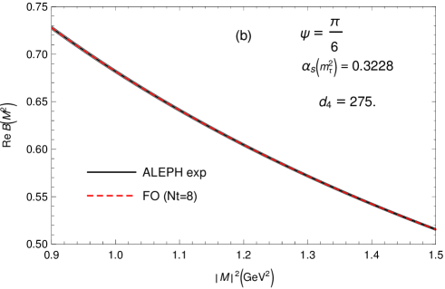
Figure 1: (coloured online) The values of ${\rm Re}B(M^{2};\sigma_{\rm m})$ along the ray $M^{2}=|M^{2}|\exp(i\Psi)$ with $\Psi=\pi/6$. The narrow grey band are the experimental predictions. The red dashed line inside the band is the result of the FOPT global fit with truncation index $N_{t}=8$. Similar fitting curves are obtained for the rays with $\Psi=0$ and $\Psi=\pi/4$.

The truncation index $N_{t}$ is then fixed by considering the first two double-pinched momenta $a^{(2,0)}(\sigma_{\rm m})$ and $a^{(2.1)}(\sigma_{\rm m})$ and requiring local stability of their values under the variation of $N_{t}$. The resulting extracted values of the coupling are

$$\alpha_{s}(m_{\tau}^{2})^{\rm(FO)} = 0.3228\pm 0.0003({\rm exp})^{-0.0026}_{+0.0070}(\kappa)^{-0.0103}_{+0.0079}(d_{4})^{+0.0081}_{-0.0057}(N_{t})$$ (9)

$$= 0.3228^{+0.0134}_{-0.0121}\approx 0.323^{+0.013}_{-0.012}\qquad(N_{t}=8^{+2}_{-3}).$$

$$\alpha_{s}(m_{\tau}^{2})^{\rm({\widetilde{\rm FO}})} = 0.3209\pm 0.0003({\rm exp})^{-0.0038}_{+0.0201}(\kappa)^{-0.0039}_{+0.0047}(d_{4})^{+0.0293}_{-0.0084}(N_{t})$$ (10)

$$= 0.3209^{+0.0359}_{-0.0100}\approx 0.321^{+0.036}_{-0.010}\qquad(N_{t}=5\pm 2).$$

$$\alpha_{s}(m_{\tau}^{2})^{\rm(PV)} = 0.3269\pm 0.0003({\rm exp})^{+0.0007}_{+0.0102}(\kappa)^{-0.0064}_{+0.0155}(d_{4})^{+0.0092}_{-0.0006}(N_{t})^{+0.0167}_{-0.0067}({\rm amb})$$ (11)

$$= 0.3269^{+0.0266}_{-0.0093}\approx 0.327^{+0.027}_{-0.009}\qquad(N_{t}=8^{+2}_{-3}).$$

$$\alpha_{s}(m_{\tau}^{2})^{\rm(CI)} = 0.3488\pm 0.0005({\rm exp})^{+0.0078}_{+0.0004}(\kappa)\pm 0.0000(d_{4})^{-0.0027}_{+0.0119}(N_{t})$$ (12)

$$= 0.3488^{+0.0142}_{-0.0028}\approx 0.349^{+0.014}_{-0.003}\qquad(N_{t}=4^{+2}_{-1}).$$

The uncertainties were presented as separate terms. The variation of the renormalisation scale parameter $\kappa\equiv\mu^{2}/Q^{2}$ was taken in the range $2/3\leq\kappa\leq 2$ ($\kappa=1$ for the central values). The truncation index is $N_{t}=8,5,8$ for the central cases of FO, ${\widetilde{\rm FO}}$ and PV.

The (truncated) Contour improved perturbation theory (CIPT) results were also included in the above results, for comparison. However, the truncated CIPT approach for $d(Q^{2})_{D=0}$ evaluation appears to require a different type of OPE in the $D>0$ part of the contributions, because the renormalon structure and the related renormalon ambiguities are not reflected in the truncated CIPT series Hoang:2021nlz . We thus include only FO, ${\widetilde{\rm FO}}$ and PV results in the average

$$\alpha_{s}(m_{\tau}^{2}) = 0.3235^{+0.0138}_{-0.0126}\qquad({\rm FO}+{\widetilde{\rm FO}}+{\rm PV})$$

$$\Rightarrow\;\alpha_{s}(M_{Z}^{2}) = 0.1191\pm 0.0016.$$ (13)

In Table 1 we compare these results with some other results in the literature.

Table 1: The values of $\alpha_{s}(m_{\tau}^{2})$, extracted by various groups applying sum rules and various methods to the ALEPH $\tau$-decay data.

group	sum rule	FO	CI	PV	average
Baikov et al.,2008 Baikov:2008jh	$a^{(2,1)}=r_{\tau}$	$0.322\pm 0.020$	$0.342\pm 0.011$	—	$0.332\pm 0.016$
Beneke&Jamin, 2008 Beneke:2008ad	$a^{(2,1)}=r_{\tau}$	$0.320^{+0.012}_{-0.007}$	—	$0.316\pm 0.006$	$0.318\pm 0.006$
Caprini, 2020 Caprini:2020lff	$a^{(2,1)}=r_{\tau}$	—	—	$0.314\pm 0.006$	$0.314\pm 0.006$
Davier et al., 2013 Davier:2013sfa	$a^{(i,j)}$	$0.324$	$0.341\pm 0.008$	—	$0.332\pm 0.012$
Pich&R.Sánchez, 2016 Pich:2016bdg	$a^{(i,j)}$	$0.320\pm 0.012$	$0.335\pm 0.013$	—	$0.328\pm 0.013$
Boito et al., 2014 Boito:2014sta	DV in $a^{(i,j)}$	$0.296\pm 0.010$	$0.310\pm 0.014$	—	$0.303\pm 0.012$
our prev. work, 2021 Ayala:2021mwc	BL ($O_{6},O_{8}$)	$0.308\pm 0.007$	—	$0.316^{+0.008}_{-0.006}$	$0.312\pm 0.007$
this work, 2022 (also Ayala:2021yct )	BL ($O_{6}^{(1)},O_{6}^{(2)}$)	$0.323^{+0.013}_{-0.012}$(FO)	—	$0.327^{+0.027}_{-0.009}$	$0.324\pm 0.013$
		$0.321^{+0.021}_{-0.030}$(${\widetilde{\rm FO}}$)

The results Eq. (13) can get significantly affected when the assumptions or methods are changed. For example, if we chose, instead of the central value $d_{4}=275.$, the upper upper bound $d_{4}=338.$ of Eq. (7) as the central value, the results would decrease somewhat, to $\alpha_{s}(m_{\tau}^{2})\approx 0.320\pm 0.015$ [$\alpha_{s}(M_{Z}^{2})\approx$ $0.1187^{+0.0016}_{-0.0019}$], i.e., $\delta\alpha_{s}(m^{2}_{\tau})\approx-0.004$.

If we took, instead of the two mentioned $D=6$ terms in the OPE, the simple $D=6$ and $D=8$ OPE terms [$\sim 1/(Q^{2})^{3}$ and $\sim 1/(Q^{2})^{4}$], the central value would decrease by about $\delta\alpha_{s}(m^{2}_{\tau})\approx-0.008$. In our previous work Ayala:2021mwc we used the OPE with simple $D=6,8$ terms, and took for $d_{4}$ higher values $d_{4}=338\pm 63$ than here Eq. (7).

If we took $N_{t}=5$ in all three methods (i.e., no extension of Adler function beyond $d_{4}a^{5}$), then the central value of $\alpha_{s}(m_{\tau}^{2})$ in FO changes from $0.3288$ to $0.3171$, and in PV from $0.3269$ to $0.3277$ $\Rightarrow$ for the average of the three methods the central value changes from $0.3235$ to $0.3219$ [$\alpha_{s}(M_{Z}^{2})$ from $0.1191$ to $0.1189$], i.e., $\delta\alpha_{s}(m^{2}_{\tau})=-0.0016\approx-0.002$, small.

According to the results (9)-(11), Borel-Laplace sum rules indicate that the theoretical uncertainties dominate over the experimental ones. Part of these theoretical uncertainties would be reduced by: 1.) the calculation of the five-loop Adler function coefficient $d_{4}$; 2.) the use of the more complicated structure of the $D=6$ OPE terms Boito:2015joa and the corresponding terms in the $D=0$ $u=3$ IR renormalon structure; 3.) the use of a variant of the QCD coupling $a(Q^{2})$ without the Landau singularities in the $D=0$ contribution, because this would allow for the resummation to all orders (no truncation) of the renormalon-motivated contribution $D=0$ and would eliminate the renormalisation scale ambiguity ($\kappa$). The high precision ALEPH determination of the $\tau$ spectral function represents an important source of data for understanding better the behaviour of QCD at the limit between the perturbative and nonperturbative regimes.

References

(1)
P. A. Baikov, K. G. Chetyrkin and J. H. Kühn,
Phys. Rev. Lett. 101 (2008), 012002.
(2)
A. L. Kataev and V. V. Starshenko,
Mod. Phys. Lett. A 10, 235 (1995).
(3)
D. Boito, P. Masjuan and F. Oliani,
JHEP 1808, 075 (2018).
(4)
M. Beneke and M. Jamin,
JHEP 09 (2008), 044.
(5)
G. Cvetič,
Phys. Rev. D 99 (2019) no. 1, 014028.
(6)
D. Boito, D. Hornung and M. Jamin,
JHEP 12 (2015), 090.
(7)
C. Ayala, G. Cvetič, R. Kögerler and I. Kondrashuk,
J. Phys. G 45 (2018) no.3, 035001.
(8)
A. H. Hoang and C. Regner,
The European Physical Journal Special Topics 230 (2021) no.12, 2625
[arXiv:2105.11222 [hep-ph]].
(9)
I. Caprini,
Phys. Rev. D 102 (2020) no.5, 054017.
(10)
M. Davier, A. Höcker, B. Malaescu, C. Z. Yuan and Z. Zhang,
Eur. Phys. J. C 74 (2014) no.3, 2803.
(11)
A. Pich and A. Rodríguez-Sánchez,
Phys. Rev. D 94 (2016) no.3, 034027.
(12)
D. Boito, M. Golterman, K. Maltman, J. Osborne and S. Peris,
Phys. Rev. D 91 (2015) no.3, 034003.
(13)
C. Ayala, G. Cvetič and D. Teca,
Eur. Phys. J. C 81 (2021) no.10, 930.
(14)
C. Ayala, G. Cvetič and D. Teca,
[arXiv:2112.01992 [hep-ph]].