The analytic structure of the fixed charge expansion

Abstract

We investigate the analytic properties of the fixed charge expansion for a number of conformal field theories in different space-time dimensions. The models investigated here are $O(N)$ and $QED_{3}$. We show that in $d=3-\epsilon$ dimensions the contribution to the $O(N)$ fixed charge $Q$ conformal dimensions obtained in the double scaling limit of large charge and vanishing $\epsilon$ is non-Borel summable, doubly factorial divergent, and with order $\sqrt{Q}$ optimal truncation order. By using resurgence techniques we show that the singularities in the Borel plane are related to worldline instantons that were discovered in the other double scaling limit of large $Q$ and $N$ of Ref. Dondi:2021buw . In $d=4-\epsilon$ dimensions the story changes since in the same large $Q$ and small $\epsilon$ regime the next order corrections to the scaling dimensions lead to a convergent series. The resummed series displays a new branch cut singularity which is relevant for the stability of the $O(N)$ large charge sector for negative $\epsilon$. Although the $QED_{3}$ model shares the same large charge behaviour of the $O(N)$ model, we discover that at leading order in the large number of matter field expansion the large charge scaling dimensions are Borel summable, single factorial divergent, and with order $Q$ optimal truncation order.
 
Preprint: RBI-ThPhys-2022-6

I Introduction

Our understanding of Nature is seriously hampered by our limited knowledge of quantum field theory (QFT) in the strongly coupled regime. Time-honoured examples range from Quantum Chromodynamics (QCD) to the understanding of critical dynamics relevant for a plethora of physical applications from condensed matter physics Cardy:1996xt to epidemiology DellaMorte:2020wlc ; 10.3389/fams.2021.659580 ; cacciapaglia2021epidemiological ; cacciapaglia2020second ; Cacciapaglia:2021vvu . Several tools have been developed to tackle strongly coupled dynamics including using weakly coupled expansions to deduce non-perturbative information, see for example LeGuillou:1990nq for a review. Being, in general, the perturbative series asymptotic, the non-perturbative information is expected to be contained in the analytic structure of their Borel transform. A well-known example is given by instantons singularities in the Borel plane, which have a semiclassical interpretation in terms of non-trivial classical trajectories Lipatov:1976ny . The mathematical framework that systematizes the idea of inferring non-perturbative physics from perturbation theory was developed by J. Ecalle in the ${}^{\prime}80$s Ecalle and takes the name of resurgence theory . In the last years, many works have successfully applied these ideas to QFT Dunne:2012ae ; Dunne:2012zk ; Argyres:2012ka ; Cherman:2014ofa ; Dorigoni:2015dha ; Behtash:2015kna ; Yamazaki:2017ulc ; Boito:2017cnp ; Marino:2019eym ; Ishikawa:2019tnw ; Ishikawa:2019oga ; Bersini:2019axn ; Abbott:2020qnl ; Borinsky:2020vae ; Dunne:2021acr ; Maiezza:2021mry ; Marino:2021dzn ; Argyres:2012vv ; Dunne:2021lie providing a novel perspective on various non-perturbative phenomena such as renormalons, instantons, and quark-hadron duality. Moreover, an intimate relation has emerged between resurgence and phase transitions when the latter are seen as Stokes phenomena Pisani ; Kanazawa:2014qma ; Buividovich:2015oju ; Ahmed:2017lhl ; Fujimori:2021oqg ; Basar:2021gyi .

At the same time, an independent line of research is being developed and it is aimed at the understanding of the strongly coupled regime of conformal field theories (CFT)s via a large-charge induced semiclassical expansion Hellerman:2015nra . Here one uses EFT methods Monin:2016jmo ; Alvarez-Gaume:2016vff ; Banerjee:2017fcx ; Hellerman:2017sur ; delaFuente:2018qwv ; Orlando:2019hte ; Banerjee:2019jpw ; Cuomo:2020rgt ; Cuomo:2021ygt ; Hellerman:2021yqz ; Cuomo:2021cnb ; Pellizzani:2021hzx ; Hellerman:2021qzz ; Banerjee:2021bbw . In fact, semiclassical expansions have shown to be useful even in resumming infinite series of Feynman diagrams thereby helping shed light on higher order computations in different regimes Alvarez-Gaume:2019biu ; Badel:2019oxl ; Badel:2019khk ; Antipin:2020abu ; Antipin:2020rdw ; Antipin:2021akb ; Antipin:2021jiw ; Arias-Tamargo:2019xld ; Arias-Tamargo:2020fow ; Jack:2020wvs ; Jack:2021ypd ; Jack:2021lja ; Jack:2021ziq ; Giombi:2020enj ; Giombi:2021zfb ; Araujo:2021sjv ; Rodriguez-Gomez:2022gbz . The approach can be extended to non-conformal QFTs as illustrated in Son:1995wz ; Orlando:2019skh ; Orlando:2020yii ; Moser:2021bes ; Orlando:2021usz , with possible physical applications such as the study of multi-boson production processes in the Standard Model.

The potential effectiveness of the large-charge expansion for small values of the charge, that seems to emerge by comparing predictions to lattice results Banerjee:2017fcx ; Banerjee:2019jpw , partially motivated the first analysis implementing resurgence for the large-charge expansion of Dondi:2021buw . An interesting investigation of the exponentially small corrections to the large R-charge expansion in $\mathcal{N}=2$ superconformal QCD appeared a few weeks later in Hellerman:2021duh . In Dondi:2021buw , the authors considered the spectrum of charge $Q$ operators for the critical $O(N)$ model in $d=3$ dimensions in the double-scaling limit

$$Q\to\infty\,,\qquad N\to\infty\,,\qquad\frac{Q}{N}\text{~{}~{}~{}fixed}\,.$$ (1)

In this limit, the scaling dimensions of the lowest-lying operators with total charge $Q$ assume the form Alvarez-Gaume:2019biu

$$\Delta_{Q}=\sum_{j=-1}\frac{1}{N^{j}}\Delta_{j}\left(\frac{Q}{N}\right)\,.$$ (2)

By expanding the $\Delta_{j}$ in the small $\frac{Q}{N}$ limit, one recovers the ordinary $1/N$ expansion Moshe:2003xn , while for ${Q}/{N}\gg 1$, Eq.(2) reproduces the general form of the large-charge expansion in generic non-supersymmetric relativistic CFTs Hellerman:2015nra ; Monin:2016jmo ; Cuomo:2020rgt

$$\Delta_{Q}=Q^{\frac{d}{d-1}}\left[\alpha_{1}+\alpha_{2}Q^{\frac{-2}{d-1}}+\alpha_{3}Q^{\frac{-4}{d-1}}+\ldots\right]+Q^{0}\left[\beta_{0}+\beta_{1}Q^{\frac{-2}{d-1}}+\ldots\right]+\mathcal{O}\left(Q^{-\frac{d}{d-1}}\right)\ ,$$ (3)

which can be derived from the large-charge effective action without assuming the presence of other expansion parameters apart from $1/Q$. The central object studied in Dondi:2021buw is the functional determinant of a free scalar field with mass equal to the chemical potential $\mu$ (conjugated to the fixed charge $Q$) on $\mathbb{R}\times S^{d-1}$

$$\log\left(\det\left(-\partial_{0}^{2}-\Delta_{S^{d-1}}+\mu^{2}\right)\right)=\sum_{\ell=0}n_{\ell}\sqrt{J_{\ell}^{2}+\mu^{2}}\,,$$ (4)

where $\Delta_{S^{d-1}}$ is the Laplacian on the $(d-1)$-sphere, whose eigenvalues $J^{2}_{\ell}$ and their multiplicity $n_{\ell}$ are given by

$$J^{2}_{\ell}=\ell(\ell+d-2)\,,\qquad n_{\ell}=\frac{(2\ell+d-2)\Gamma(\ell+d-2)}{\Gamma(\ell+1)\Gamma(d-1)}\,.$$ (5)

In fact, for technical reasons, the theory is Weyl-mapped to $\mathbb{R}\times S^{d-1}$, and, via the state operator correspondence Cardy:1984rp ; Cardy:1985lth , the energy levels on the cylinder are linked to the associated spectrum of scaling dimensions. $\Delta_{-1}$ in Eq.(2) is then obtained as the Legendre transform of Eq.(4) with respect to the chemical potential to express it in terms of the fixed charge $Q$.

The small $\frac{Q}{N}$ expansion of $\Delta_{-1}$ is convergent with a radius of convergence related to the appearance of a zero-mode in the spectrum. On the other hand, the large $\frac{Q}{N}$ expansion of $\Delta_{-1}$ diverges $(2n)!$ factorially, and its Borel transform exhibits an infinite number of singularities on the positive real axis which, according to resurgence theory , indicate the emergence of non-perturbative corrections. The leading non-perturbative contributions scale as $e^{-\sqrt{Q}}$ and stem from worldline instantons describing the geodesic motion of a free particle with mass $\mu$ moving on close trajectories Schubert:2001he . Since these corrections originate from the geometrical properties of the compactification manifold, the authors of Dondi:2021buw conjectured the above to be a general property of the large-charge expansion in the three-dimensional $O(N)$ CFT. It was envisioned to be a consequence of the effective action describing the large-charge sector of the theory that is by itself an asymptotic series. The resulting optimal truncation order, for any $N$, is $n_{\text{opt}}\approx\sqrt{Q}$ with the related error $\mathcal{O}\left(e^{-\sqrt{Q}}\right)$. The $O(N)$ model in $d=5$ in the same double-scaling limit has been investigated in Moser:2021bes , reaching similar conclusions. Here we add information on the convergence properties of the large-charge expansion by addressing various models displaying very different large order behaviours. Along our journey, we will encounter convergent, asymptotic but Borel summable, and non-Borel summable series; in the first case we will investigate what one can learn on the physics of the expansion from a finite number of coefficients. To this end, our main tool will be the Darboux’s theorem Darboux ; Darboux2 , which relates the behaviour of a function around its non-analytical points to the rate of growth of the coefficients of its series expansion around regular points. Physical applications were explored in Darboux ; Frazer:1961zz ; Hunter:1973zz ; Kazakov:1978ey ; Fischer:1997bs ; Stephanov:2006dn ; Caprini:2017ikn ; Dondi:2019ivp ; Costin:2020hwg ; Dondi:2020qfj .

We organize the work as follows. In Sec.II, we consider the critical $g^{2}(\phi_{i}\phi_{i})^{3}$ theory in $d=3-\epsilon$, which has been investigated in Badel:2019khk ; Jack:2020wvs in the double-scaling limit

$$Q\to\infty\,,\qquad g\to 0\,,\qquad gQ=\text{fixed}\,.$$ (6)

resulting in the following semiclassical expansion

$$\Delta_{Q}=\sum_{j=-1}^{\infty}g^{*j}\Delta_{j}(g^{*}Q)\ .$$ (7)

We discover that the small-charge (i.e. the small $gQ$) expansions of $\Delta_{-1}$ and $\Delta_{0}$ are convergent and share the same radius of convergence. We observe that, as in Dondi:2021buw , the leading singularity, which is an algebraic branch point, occurs when the mass of a certain mode vanishes. Moreover, the small $gQ$ expansion of $\Delta_{0}$ provides an interesting example of how the program of reconstructing the analytic structure of a function from a limited number of expansion coefficients can fail. In fact, even the precise identification of the radius of convergence requires more than one hundred expansion coefficients. However, we are able to make progress by identifying the source of the problem in the occurrence of two coincident singularities for which we can disentangle their contributions.

Additionally, $\Delta_{0}$ in Eq.(7) is the functional determinant of the fluctuations around the classical solution and, in $O(N)$-invariant theories in any $d$, receives contributions from three types of modes Alvarez-Gaume:2016vff ; Antipin:2020abu : one massless conformal mode, one massive radial mode, and $N-2$ spectator modes. The computation of the large $gQ$ expansion of the full $\Delta_{0}$ is technically challenging and the approaches considered in the literature resorted to numerical fits delaFuente:2018qwv ; Badel:2019oxl ; Badel:2019khk ; Jack:2020wvs ; Jack:2021ypd and numerical evaluation of integrals Cuomo:2021cnb , in order to determine the first few coefficients. For the sake of simplicity, in this exploratory work we focus only on the contribution of the spectator modes, which is given by the functional determinant (4) in $d=3$ i.e. it is exactly the same object considered in Dondi:2021buw . At the same time, due to the different double-scaling limit considered, our large-charge expansion of Eq.(4) differs from the one considered in Dondi:2021buw but, not surprisingly, share all its features i.e. a $(2n)!$ factorial growth of the coefficients related to the same non-perturbative effects driven by worldline instantons. We are, therefore, able to confirm the results of Dondi:2021buw in a different double-scaling limit, providing strong evidence for the non-perturbative corrections due to worldline instantons being a general feature of the large-charge expansion on $\mathbb{R}\times S^{2}$.

Motivated by the geometrical origin of these non-perturbative corrections, in Sec.III, we move to $\mathbb{R}\times S^{3-\epsilon}$ and study the $g(\phi_{i}\phi_{i})^{2}$ $O(N)$ model in $d=4-\epsilon$ dimensions in the double-scaling limit (6), which has been previously considered in Badel:2019oxl ; Antipin:2020abu ; Jack:2021ypd . In particular, an interesting diagrammatic argument that links the large order behaviour of the coefficients of the small $gQ$ expansion of $\Delta_{j}$ for different $j$ has been given in Badel:2019oxl . After elaborating the consequences of this proposal for the analytical structure of the $\Delta_{j}$, we show that the small $gQ$ expansion of $\Delta_{0}$ contradicts it; the situation is completely analogous to the $d=3-\epsilon$ case; the small $gQ$ expansion of both $\Delta_{-1}$ and $\Delta_{0}$ is convergent, with the radial mode becoming massless at the leading singular point. Moreover, $\Delta_{0}$ features two coincident leading singularities. The branch point determining the radius of convergence lies on the negative $gQ$ axis and it is, therefore, possible to smoothly continue the small-charge expansion to large positive values of the charge. On the other hand, this branch point is related to the instability of the large-charge sector of the (metastable) ultraviolet FP of the quartic $O(N)$ theory in $4<d<6$, which has been recently pointed out in Giombi:2020enj ; Antipin:2021jiw and related to a phase transition on the cylinder in Moser:2021bes . In fact, this FP can be reached by continuing the $\epsilon$-expansion to negative values of $\epsilon$ Giombi:2014iua and occurs at negative $g$. Interestingly, the type of the leading singularities in both $\Delta_{-1}$ and $\Delta_{0}$ is exactly the same in the $d=4-\epsilon$ and $d=3-\epsilon$ cases. Motivated by this observation we make a slight detour and study the small-charge expansion in the cubic $O(N)$ model in $d=6-\epsilon$ and the $U(N)\times U(M)$ model in $d=4-\epsilon$ at the leading order of the semiclassical expansion (7). Intriguingly, we discover that the structure of the leading singularity at the leading order of the semiclassical expansion is shared among all these theories, despite the differences in $d$, matter content, and symmetries.

In order to study the large $gQ$ expansion of $\Delta_{0}$, we consider the contribution of the spectator modes, leaving the remaining two modes for future work. As opposed to the three-dimensional $O(N)$ theory, we discover that the large $gQ$ expansion of these contributions converges. In the case of the spectator modes, this is traced back to the convergence of the heat kernel expansion on odd-dimensional spheres Camporesi:1990wm . Moreover, we are able to resum the large $gQ$ expansion of the contribution of the spectator modes obtaining a simple analytical expression not involving infinite sums. Its analytical structure reveals a previously unnoticed branch cut on the negative $gQ$ axis starting at $gQ=0$, which makes the fixed-charge sector of the $O(N)$ theory in $4<d<6$ unstable for any value of the charge. This differs from previous investigations Giombi:2020enj ; Antipin:2021jiw , which observed such instabilities only above a critical (finite) value of the charge.

In Sec.IV, we return to $\mathbb{R}\times S^{2}$ and study the analytical properties of the charge expansion in $QED_{3}$ with $N_{f}$ two-component complex fermions , which has been thoroughly studied in the last decades Borokhov:2002ib ; Pisarski:1984dj ; Appelquist:1988sr ; Maris:1995ns ; Nash:1989xx ; Pufu:2013vpa ; Braun:2014wja ; Giombi:2015haa ; Chester:2016wrc ; Albayrak:2021xtd ; Gusynin:2016som due to its relevance for condensed matter (especially for the description of algebraic spin liquids Rantner:2002zz ) and its similarities with $QCD$ in four dimensions. In particular, we focus on the scaling dimension $\Delta_{Q}$ of charge-$Q$ monopole operators, which create topological disorder by acting in a given position of the space-time Borokhov:2002ib . In general, their proliferation (occurring when the monopoles are relevant operators in the RG sense) confines the gauge field Polyakov:1975rs ; Polyakov:1976fu , but the screening produced by the fermions can elude confinement and realize conformal dynamics in the infrared above a critical value of $N_{f}$, $0<N_{f,\text{crit}}<10$ Appelquist:1988sr ; Nash:1989xx ; Gusynin:2016som ; Braun:2014wja . By virtue of the state-operator correspondence, the scaling dimensions of monopole operators equal the ground state energy of the theory on $R\times S^{2}$ in the presence of $4\pi Q$ magnetic flux across $S^{2}$. The ground state energy can then be computed semiclassically in the $1/N_{f}$ expansion resulting in

$$\Delta_{Q}=\sum_{j=-1}^{\infty}\frac{1}{N_{f}^{j}}\Delta_{j}(Q)\,,$$ (8)

where $\Delta_{-1}$ and $\Delta_{0}$ have been computed, respectively, in Borokhov:2002ib and Pufu:2013vpa . It can be shown that the large-$Q$ expansion of $\Delta_{Q}$ reproduces the general large-charge formula (3), including the correct value of the universal term scaling as $Q^{0}$ Hellerman:2015nra . Here, the relevant eigenfunctions on $S^{2}$ are given in terms of monopole harmonics Wu:1976ge ; Wu:1977qk , generalizing the spherical harmonics in the presence of the field generated by a magnetic monopole. Interestingly, the properties of these harmonics (in particular the fact that their angular momentum is bounded from below by the charge) lead to considerable differences with respect to the $O(N)$ theory on $\mathbb{R}\times S^{2}$. In fact, we find that the large-$Q$ expansion of $\Delta_{-1}$ is only $n!$ (and not $(2n)!$) factorially divergent, with an optimal truncation order $n_{\text{opt}}\approx Q$ and related error of order $\mathcal{O}\left(e^{-Q}\right)$. Moreover, the Borel transform $\mathcal{B}[\Delta_{-1}](t)$ exhibits an infinite series of equally spaced branch points at $t=4\pi m\ i$, $m\in\mathbb{Z}$, and, therefore, is Borel summable. The Borel sum is given in terms of an infinite sum of modified Bessel functions of the second kind, providing an alternative expression for $\Delta_{-1}$. Notice that, due to the properties of the ground state, at the leading order in $1/N_{f}$ the addition of a Gross-Neveu (GN) interaction term does not affect $\Delta_{Q}$ Dupuis:2021flq . Therefore, our findings trivially apply also to the critical $QED_{3}-GN$ model, which is relevant for the quantum phase transition between Dirac and chiral spin liquids He:2013wcz ; He:2015vnc ; Janssen:2017eeu . Finally, we give our conclusions in Sec.V.

II The $O(N)$ model in $d=3-\epsilon$

In this section, we consider the sextic $O(N)$ CFT in $d=3-\epsilon$ with the Lagrangian

$${\cal L}=\frac{1}{2}\partial^{\mu}\phi_{i}\partial_{\mu}\phi_{i}+\frac{g^{2}}{8\times 3!}(\phi_{i}\phi_{i})^{3}.$$ (9)

where $\phi_{i}$, $i=1,\dots,N$, transforms as a $O(N)$-vector. This model exhibits an infrared stable fixed point at Pisarski:1982vz

$$\frac{g^{2}}{(4\pi)^{2}}=\frac{2\epsilon}{22+3N}+\mathcal{O}\left(\epsilon^{2}\right)\,.$$ (10)

Interestingly, the beta function of the $g$ coupling is non vanishing from two-loops, and the model is, therefore, conformally invariant in $d=3$ at the one-loop level. This property will allow us to directly compare our results to those in Dondi:2021buw and link them to the large-charge effective theory describing the three-dimensional $O(N)$ CFT. In Jack:2020wvs , the scaling dimension of the lowest-lying operators with total charge $Q$ has been computed in the double-scaling limit (6), where one can perform the semiclassical expansion of (7). The leading order $\Delta_{-1}$ is given by evaluating the action on the non-trivial classical trajectory induced by fixing the charge and it reads

$$\Delta_{-1}(gQ)=gQF_{-1}\left(\frac{g^{2}Q^{2}}{2\pi^{2}}\right)\,,\quad F_{-1}(x)=\frac{1+\sqrt{1+x}+\tfrac{x}{3}}{\sqrt{2}(1+\sqrt{1+x})^{\frac{3}{2}}}\,,\quad x=\frac{g^{2}Q^{2}}{2\pi^{2}}\ .$$ (12)

At the next-to-leading order of the semiclassical expansion (7), one needs to compute the functional determinant of the fluctuations around the classical solution. This can be formally written as

$$\Delta_{0}(gQ)=\Delta_{0}^{(a)}(gQ)+\left(\frac{N}{2}-1\right)\Delta_{0}^{(b)}(gQ)\,,$$ (13)

with

$$\Delta_{0}^{(a)}(gQ) =\frac{1}{2}\sum_{\ell=0}^{\infty}n_{\ell}[\omega_{+}(\ell)+\omega_{-}(\ell)]\,,$$ (14)

$$\Delta_{0}^{(b)}(gQ) =\sum_{\ell=0}^{\infty}n_{\ell}\ \omega_{*}(\ell)\,.$$ (15)

Here

$$\omega_{\pm}^{2}(\ell)=J_{\ell}^{2}+2\left(2\mu^{2}-\frac{(d-2)^{2}}{4}\right)\pm 2\sqrt{J_{\ell}^{2}\mu^{2}+\left(2\mu^{2}-\frac{(d-2)^{2}}{4}\right)^{2}}\,,\qquad\omega_{*}(\ell)=\sqrt{J_{\ell}^{2}+\mu^{2}}\,,$$ (16)

are the dispersion relations of the spectrum. The latter contains a massless mode $\omega_{-}$, (the conformal mode), a gapped mode $\omega_{+}$ with mass $\omega_{+}(0)=2\sqrt{2\mu^{2}-\frac{(d-2)^{2}}{4}}$ (the radial mode) as well as $(N-2)$ gapped modes $\omega_{*}$ with mass $\omega_{*}(0)=\mu$ (the spectator modes). The above expressions are explicit functions of the chemical potential $\mu$, which is related to the ’t Hooft coupling $gQ$ through the equations of motion as

$$\mu=\frac{1}{2\sqrt{2}}\sqrt{1+\sqrt{1+\frac{g^{2}Q^{2}}{2\pi^{2}}}}\,.$$ (17)

After regularizing the sums over $\ell$ in Eq.(15), one obtains the following final expression for the functional determinants Jack:2020wvs

$$\Delta_{0}^{(a)}(gQ) =\frac{1}{4}-3\mu^{2}+\tfrac{1}{2}\sqrt{8\mu^{2}-1}+\frac{1}{2}\sum_{\ell=1}^{\infty}\sigma^{(a)}(\ell)\,,$$ (18)

$$\Delta_{0}^{(b)}(gQ) =-\frac{1}{4}-\mu^{2}+\mu+\frac{1}{2}\sum_{\ell=1}^{\infty}\sigma^{(b)}(\ell)\,,$$ (19)

where

$$\sigma^{(a)}(\ell)= (1+2\ell)[\omega_{+}(\ell)+\omega_{-}(\ell)]-4l(l+1)-6\mu^{2}+\frac{1}{2}\,,$$ (20)

$$\sigma^{(b)}(\ell)= 2(1+2\ell)\omega_{*}(\ell)-4l(\ell+1)-2\mu^{2}-\frac{1}{2}\,,$$ (21)

are convergent sums.

II.1 The small-charge expansion

Equipped with the basic setup above we can now study the convergence properties of the small $gQ$ expansion of $\Delta_{-1}$ (12) and $\Delta_{0}$ (13). In this limit, $\Delta_{-1}$ is convergent with a radius of convergence determined by the only non-analytical point at $x_{0}=-1$. It is therefore instructive to determine how many coefficients of the small $gQ$ expansion are needed in order to fully characterize the singularity. This is achieved by making use of the Darboux’s theorem which links the large order behaviour of the expansion coefficients about one point (which we take to be $x=0$) to the behaviour of the function in the vicinity of its singularities. Concretely, if the perturbative coefficients of a function $\mathcal{O}(x)=\sum c_{n}x^{n}$ grow as

$$c_{n}\sim\frac{1}{x_{0}^{n}}\left[f(x_{0})\binom{n+p-1}{n}-x_{0}f^{\prime}(x_{0})\binom{n+p-2}{n}+\frac{x_{0}^{2}}{2!}f^{\prime\prime}(x_{0})\binom{n+p-3}{n}-\dots\right]+\dots\,,$$ (22)

then $x_{0}$ corresponds to the closest singularity to the origin and further determines the radius of convergence of the expansion around $x=0$. Moreover, in the vicinity of $x_{0}$, $\mathcal{O}(x)$ behaves as

$$\mathcal{O}(x)=f(x)\left(1-\frac{x}{x_{0}}\right)^{-p}+\text{analytic}\,,\qquad x\to x_{0}\,,$$ (23)

with $f(x)$ an analytic function near $x_{0}$. Given the $c_{n}$, the parameters entering Eq.(22) can be determined by considering various sequences which tend to them in the limit $n\to\infty$ and making use of acceleration methods to improve the convergence. For instance, the ratio of consecutive coefficients $c_{n}/c_{n-1}$ converges to $1/x_{0}$ as $n\to\infty$ , whereas $p$ and $f(x_{0})$ can be found by considering the following sequences

$$p=1+\lim_{n\to\infty}n\left(x_{0}\frac{c_{n}}{c_{n-1}}-1\right)\,,$$ (24)

$$f(x_{0})=\lim_{n\to\infty}\frac{c_{n}}{\left(\frac{1}{x_{0}}\right)^{n}\binom{n+p-1}{n}}\,.$$ (25)

In a similar manner, one can determine all the derivatives $f^{(n)}(x_{0})$ and relevant parameters characterizing the subleading singularities Darboux ; Darboux2 ; Dorigoni:2015dha . As summarized in Table 1, by analyzing $20$ coefficients of the small-charge expansion of $\Delta_{-1}$, we learn that they satisfy Eq.(22) with $x_{0}=-1$, $p=-3/2$, $f(x_{0})=-\frac{1}{12\sqrt{2}}$. With the same number of coefficients, we find also that $f^{\prime}(x_{0})=-0.051559(1)$, while computing higher derivatives of $f(x)$ requires an increasing number of coefficients. For instance, to obtain $f^{\prime\prime}(x_{0})=-0.091150(1)$ and $f^{\prime\prime\prime}(x_{0})=-0.2467(1)$, we had to consider $46$ and $89$ coefficients, respectively. .

	small $Q\epsilon$						large $Q\epsilon$
	$O(N)$ in $d=3-\epsilon$			$O(N)$ in $d=4-\epsilon$			$O(N)$ in $d=3-\epsilon$	$O(N)$ in $d=4-\epsilon$
$\Delta_{j}$	$\Delta_{-1}$	$\Delta_{0}^{(a)}$	$\Delta_{0}^{(b)}$	$\Delta_{-1}$	$\Delta_{0}^{(a)}$	$\Delta_{0}^{(b)}$	$\Delta_{-1}$	$\Delta_{-1}$
$n$	$20$	$>100$	$22$	$25$	$>100$	$13$	$28$	$36$

Table 1: Number of expansion coefficients needed to determine, with a $5$ digits accuracy, the position ($x_{0}$), type ($p$), and amplitude $(f(x_{0}))$ of the leading singularity in the coefficient functions $\Delta_{j}$ in the $O(N)$ model in $d=3-\epsilon$ and $d=4-\epsilon$ dimensions. In the case of $\Delta_{0}$, we separate the contribution of $\Delta_{0}^{(a)}$ and $\Delta_{0}^{(b)}$ as in Eq.(13). In order to accelerate the convergence, we made use of the Richardson extrapolation Richpaper , which in all cases performed better than other series acceleration methods, e.g. Shanks transforms Shanks and Padé approximants.

Physically, when $x=x_{0}$ the chemical potential takes the value $\mu(x_{0})=\frac{1}{2\sqrt{2}}$ and the mass of the radial mode $\omega_{+}$ vanishes in $d=3$. Therefore, as in the large-$N$ analysis of Dondi:2021buw , the radius of convergence is dictated by the requirement of positive masses.

In order to study the small $gQ$ expansion of $\Delta_{0}$ we consider separately $\Delta_{0}^{(a)}=\sum_{n=0}a_{n}^{(a)}x^{n}$ and $\Delta_{0}^{(b)}=\sum_{n=0}a_{n}^{(b)}x^{n}$. In the $\Delta_{0}^{(a)}$ case, the ratio test to determine the radius of convergence exhibits a slow convergence while the sequence (25), fails to converge even with more than one hundred coefficients. The poor performance of the approach can be understood simply by inspecting the $\mu(x)$ dependence of $\Delta_{0}^{(a)}$ in Eq. (18). Here one immediately observes the emergence of two different singular behaviour at $x_{0}$, one coming from the square root term (3rd term) that has a branch cut that goes like $(1+x)^{1/4}$ (corresponding to $p=-1/4$) while the rest of the expression has an expected branch cut that goes like $(1+x)^{1/2}$ (corresponding to $p=-1/2$) . Making use of this knowledge we can accelerate the convergence process. We conclude that the slow convergence of Eq.(25) when considering the full $a_{n}^{(a)}$ is due to the presence of two coincident singularities . Being all the terms in Eq.(19), regular in $\mu(x_{0})$ the convergence of the various ratio tests is much higher in the $\Delta_{0}^{(b)}$ case as shown in Table 1. We conclude that near $x_{0}=-1$, $\Delta_{0}$ behaves as

$$\Delta_{0}=f(x)\left(1+x\right)^{1/4}+g(x,N)\left(1+x\right)^{1/2}+\text{analytic}\,.$$ (26)

II.2 The large-charge expansion

As shown above, the small $gQ$ expansion of $\Delta_{-1}$ and $\Delta_{0}$ is convergent. Here, we move to investigate the large $gQ$ expansion, which, as we shall see, in the case of $\Delta_{0}$ is asymptotic and non-Borel summable. The large $gQ$ expansion of $\displaystyle{\Delta_{-1}=gQx^{1/4}\sum_{n=-0}b_{n}x^{-n/2}}$ is convergent as can be seen from the ratio of consecutive coefficients, which is depicted in Fig.1. The radius of convergence is again determined by the singularity at $x_{0}=-1$.

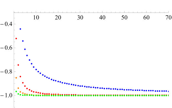
Figure 1: In this figure, we show the ratio of consecutive coefficients $\frac{b_{n}}{b_{n-1}}$ of the large $gQ$ expansion of $\Delta_{-1}$ for growing $n$. The blue line represents the original coefficients, while the red, orange, and green lines denote, respectively, the first three Richardson extrapolations. The ratio tends to the value $1/x_{0}=-1$.

The number of coefficients one needs to precisely characterize the singularity is similar to the small $gQ$ case, as shown in Table 1.

For the large $gQ$ expansion of $\Delta_{0}$ we focus on analytically determining the large-charge expansion of $\Delta_{0}^{(b)}$ and leave $\Delta_{0}^{(a)}$ for future work. As we shall see later, due to the factor of $N$ in Eq.(13), our conclusions will not be affected by the inclusion of radial and conformal modes. In order to compute the large $\mu$ expansion of $\Delta_{0}^{(b)}$, we follow Jack:2020wvs and separate the positive powers of $\mu$ as

$$\Delta_{0}^{(b)}=a_{-3}\mu^{3}+a_{-1}\mu+\sum_{l=0}(2\ell+1)\sqrt{\mu^{2}+\ell(\ell+1)}\,.$$ (27)

The value of $a_{-3}=-2/3$ and $a_{-1}=1/3$ has been computed in Jack:2020wvs by performing a numerical fit to $\Delta_{0}^{(b)}$ and will be confirmed below via an analytical computation. By Taylor-expanding the square root and exchanging the two sums, we have

$$\Delta_{0}^{(b)} =a_{-3}\mu^{3}+a_{-1}\mu+\sum_{\ell=0}(2\ell+1)\sqrt{\mu^{2}+\ell(\ell+1)}$$

$$=a_{-3}\mu^{3}+a_{-1}\mu+\sum_{k=0}\frac{(-1)^{k}\mu^{-2k-1}\Gamma\left(k+\frac{1}{2}\right)}{2\sqrt{\pi}\Gamma(k+2)}\sum_{\ell=0}(2\ell+1)\ell^{k+1}(\ell+1)^{k+1}$$

$$=a_{-3}\mu^{3}+a_{-1}\mu+\frac{1}{\mu}\sum_{k=0}a_{k}\mu^{-2k}\,.$$ (28)

By using that

$$\sum_{\ell=0}(2\ell+1)\ell^{k+1}(\ell+1)^{k+1} =\sum_{n=0}^{k+2}\binom{k+2}{n}\sum_{\ell=0}\ell^{k+n+1}+\sum_{n=0}^{k+1}\binom{k+1}{n}\sum_{\ell=0}\ell^{k+n+2}~{}$$

$$=\sum_{n=0}^{k+2}\frac{(-1)^{k+n+1}B_{k+n+2}}{k+n+2}\binom{k+2}{n}+\sum_{n=0}^{k+1}\frac{(-1)^{k+n}B_{k+n+3}}{k+n+3}\binom{k+1}{n}\,,$$ (29)

we obtain our final expression for the coefficients

$$a_{k}=\sum_{m=1}^{k+2}\frac{(-1)^{k+1}B_{2m}\Gamma\left(k+\frac{1}{2}\right)}{4\sqrt{\pi}m\Gamma(k+2)}\left[2\binom{k+1}{-k+2m-3}+\binom{k+1}{-k+2m-2}\right]\,.$$ (30)

The coefficients $a_{k}$ diverge double-factorially, as can be seen from the ratio $\displaystyle{\frac{a_{k+1}}{k^{2}a_{k}}}$, which is plotted in Fig.2. In fact, in the $k\to\infty$ limit, they behave as

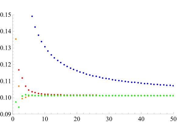
Figure 2: In this figure, we show the ratio $\frac{a_{k+1}}{k^{2}a_{k}}$ (with $a_{k}$ given by Eq.(30)) for growing $k$. The blue line represents the original ratio, while the red, orange, and green lines denote, respectively, the first three Richardson extrapolations. The ratio tends to the value $\frac{1}{\pi^{2}}=0.101321\dots$ .

$$a_{k}\approx-\pi^{-2k-5}\Gamma\left(k+\frac{1}{2}\right)\Gamma\left(k+\frac{5}{2}\right)\,.$$ (31)

We can now employ resurgence arguments to infer the non-perturbative corrections to $\Delta_{0}^{(b)}$. According to resurgence theory, given an asymptotic series $\phi^{(0)}(z)=\sum a_{k}z^{k}$, we can promote it to a transseries of the form

$$\phi(z)=\phi^{(0)}(z)+\sum_{j\neq 0}\sigma_{j}e^{-A_{j}/z^{1/\beta_{j}}}z^{-b_{j}/\beta_{j}}\Phi^{(j)}(z),\qquad\Phi^{(j)}(z)\sim\sum_{i=0}^{\infty}a_{i}^{(j)}z^{i/\beta_{j}}\,,$$ (32)

where the parameters $\beta_{j},A_{j}$ and $b_{j}$ are encoded in the large order behaviour of the $a_{k}$ coefficients as Dorigoni:2014hea ; Aniceto:2018bis

$$a_{k}\sim\sum_{j}\frac{S_{j}}{2\pi i}\frac{\beta_{j}}{A_{j}^{\beta_{j}k+b_{j}}}\sum_{i=0}^{\infty}a_{i}^{(j)}A_{j}^{i}\Gamma\left(\beta_{j}k+b_{j}-i\right)\,.$$ (33)

Therefore, the transseries can be mapped into the perturbative expansion up to a set of $j$-dependent constants $\sigma_{j}$, which are known as transseries parameters Aniceto:2018bis .

For our purposes, it is enough to focus on the dominant non-perturbative correction to the scaling dimension. The latter stems from the term with $m=k+2$ in Eq.(30). Moreover, to ease the comparison with Dondi:2021buw , we shift $k$ as $k\to k-2$ and introduce

$$\hat{a}_{k}\equiv a_{k}^{(m=k+2)}\rvert_{k\to k-2}=-\pi^{-2k-1}\Gamma\left(k+\frac{1}{2}\right)\Gamma\left(k-\frac{3}{2}\right)\zeta(2k)\,.$$ (34)

To rewrite $\hat{a}_{k}$ in the form of Eq.(33), we resort to the following identity

$$2^{2k}\Gamma(k+\tfrac{1}{2})\Gamma(k-\tfrac{3}{2}) =\sqrt{\frac{\pi}{2}}\sum_{i=0}^{\infty}\gamma_{i}\Gamma\left(2k-\frac{3}{2}-i\right)=\sqrt{\frac{\pi}{2}}\left[8\Gamma(2k-\tfrac{3}{2})+15\Gamma(2k-\tfrac{5}{2})+\frac{105}{16}\Gamma(2k-\tfrac{7}{2})+\dots\right]\,,$$ (35)

where the coefficients $\gamma_{i}$ diverge factorially and occur in Henkel’s expansion of the modified Bessel function of the second kind. After some manipulations, we obtain

$$\hat{a}_{k}=-\frac{1}{4\pi^{2}}\sum_{j=1}\frac{j^{-3/2}}{(2\pi j)^{2k-3/2}}\sum_{i=0}\gamma_{i}\Gamma\left(2k-\frac{3}{2}-i\right)\,,$$ (36)

which agrees with Eq.(33) if

$$\beta_{j}=2\,,\qquad b_{j}=-3/2\,,\qquad A_{j}=2\pi j\,,\qquad\frac{S_{j}}{2\pi i}a_{0}^{(j)}=-\frac{\gamma_{0}}{j^{3/2}8\pi^{2}}\,,\qquad a_{i>0}^{(j)}=\frac{a_{0}^{(j)}}{(2\pi j)^{i}}\frac{\gamma_{i}}{\gamma_{0}}\,.$$ (37)

Taking into account the shift in $k$ performed before, we have that the dominant non-perturbative correction to $\Delta_{0}^{(b)}$ reads

$$\Delta_{0}^{(b)}\supset\sum_{j=1}e^{-2\pi j\mu}\mu^{3/2}\sum_{i=0}a_{i}^{(j)}\mu^{-i}\,.$$ (38)

By using Eq.(17), we can rewrite the above in terms of the charge as

$$\Delta_{0}^{(b)}\supset(gQ)^{5/4}\sum_{j=1}\exp\left(-\frac{\sqrt{\pi}}{2^{3/4}}j\sqrt{gQ}\right)\sum_{i=0}a_{i}\left(2^{7/4}\sqrt{\pi}\right)^{i}(gQ)^{-i/2}\,.$$ (39)

The leading non/perturbative contribution to the scaling dimension scales as $e^{-\sqrt{Q}}$, which is the same result obtained in Dondi:2021buw for the three-dimensional $O(N)$ model in the double-scaling (2). Of course, this is not surprising, since we, similarly to Dondi:2021buw , consider the same functional determinant (4), whose transseries representation is unique. Below we will make this connection more precise and explicitly show how Eq.(39) matches the contribution of worldline instantons computed in Dondi:2021buw , corresponding to non-trivial saddle points of the geodesic equations on the two-sphere. This can be achieved by re-deriving our results using the Mellin representation of the functional determinant of the spectator modes. We, therefore, rewrite Eq.(15) as

$$\Delta_{0}^{(b)}(gQ)=\sum_{\ell=0}^{\infty}n_{\ell}\ \omega_{*}(\ell)=\sum_{\ell=0}^{\infty}(2\ell+1)\ \sqrt{\mu^{2}+\ell(\ell+1)}=\frac{1}{\Gamma(s)}\int_{0}^{\infty}dt\ t^{s-1}e^{-\mu^{2}t}\text{Tr}\left(e^{\Delta_{S^{2}}t}\right)\Bigg{\rvert}_{s=-1/2}\,.$$ (40)

Since in the limit $\mu\to\infty$, the integral over $t$ is dominated by the contribution at $t=0$, we proceed by studying the small $t$ expansion of the heat kernel $\text{Tr}\left(e^{\Delta_{S^{2}}t}\right)$. By using Poisson resummation and the asymptotic expansion of the Dawson function $F(Z)$ for $z\to\infty$, we find

$$\text{Tr}\left(e^{\Delta_{S^{2}}t}\right) =\sum_{\ell=0}^{\infty}(2\ell+1)\ e^{-\ell(\ell+1)t}=\frac{1}{2}\int_{-\infty}^{\infty}\left|\rho\right|d\rho e^{-\frac{1}{4}\left(\rho^{2}-1\right)t}+\frac{1}{2}\sum_{k=-\infty}^{\infty}(-1)^{k}\int_{-\infty}^{\infty}\left|\rho\right|d\rho e^{-\frac{1}{4}\left(\rho^{2}-1\right)t+i\pi k\rho}$$

$$=\frac{e^{t/4}}{t}+\sum_{k=-\infty}^{\infty}\frac{(-1)^{k}e^{t/4}\left(\sqrt{t}-2\pi kF\left(\frac{k\pi}{\sqrt{t}}\right)\right)}{t^{3/2}}=\frac{1}{t}\sum_{k=0}c_{k}t^{k}\,,$$ (41)

where

$$c_{k}=\sum_{n=0}^{k}\frac{2^{-2k}(-1)^{k+n+1}\left(4^{k-n}-2\right)B_{2(k-n)}}{n!(k-n)!}\,.$$ (42)

By taking the integral over $t$ in Eq.(40), one recovers the correct $a_{k}$ coefficients (30), including the coefficients of the positive powers of $\mu$ ($a_{-3}$ and $a_{-1}$) in Eq.(28). Moreover, the above shows that our expansion coefficients $a_{k}$ in Eq.(30), stems from the Cauchy product of the asymptotic expansion of Dondi:2021buw with the Taylor series of $e^{t/4}$. We again focus on the leading non-perturbative correction to the heat kernel and consider

$$c_{k}^{n=0}=\frac{(-1)^{k+1}\left(1-2^{1-2k}\right)B_{2k}}{k!}\,,$$ (43)

which, as expected, matches exactly the (full) coefficients of the heat kernel expansion in Dondi:2021buw . In particular, by using Eq.(33), we have that the leading non-perturbative corrections to the heat kernel have the following form

$$\text{Tr}\left[e^{\Delta_{S^{2}}t}\right]\,\supset\,2i\left(\frac{\pi}{t}\right)^{\frac{3}{2}}(-1)^{k+1}\rvert k\rvert e^{-(k\pi)^{2}/t}\,,$$ (44)

which, of course, precisely matches the contribution of the worldline instantons calculated in Dondi:2021buw . A few remarks are in order:

• Due to the mismatch in $N$ of the contributions of $\Delta_{0}^{(a)}$ and $\Delta_{0}^{(b)}$ to $\Delta_{0}$, the non-perturbative corrections to $\Delta_{0}^{(b)}$ found here, survive in the full $\Delta_{0}$ for every value of $N$ (except obviously $N=2$ and at most another value of $N$ for which there is an exact cancellation with $\Delta_{0}^{a}$). In addition, there may be additional non-perturbative effects coming from $\Delta_{0}^{(a)}$, which may reduce the optimal truncation order below $n_{\text{opt}}=\mathcal{O}\left(\sqrt{Q}\right)$.

• Both the authors of Ref.  Dondi:2021buw and we start from the functional determinant of the spectator modes in $d=3$ (15). However, due to the different double-scaling limits considered, we obtain two distinct expansions. Technically, we expanded Eq. (15) in powers of $\mu$ which is the mass with respect to the Laplacian operator $\Delta_{S^{2}}$, which can, in turn, be expressed as a (convergent) powers series in $Q\epsilon$ via Eq.(17). Conversely, in Dondi:2021buw , Eq.(15) is expanded in powers of the mass $m=\sqrt{\mu^{2}-\frac{(d-2)^{2}}{4}}$ with respect to the conformal Laplacian $\Delta_{S^{2}}-\frac{(d-2)^{2}}{4}$, which, in turn, can be expressed as an (asymptotic) power series in $\frac{Q}{N}$. However, the transseries representation of $\Delta_{0}^{(b)}$ derived in Dondi:2021buw via Borel resummation does not depend on such considerations and can be obtained from Eq.(40) by rewriting the heat kernel expansion as $\displaystyle{\text{Tr}\left(e^{\Delta_{S^{2}}t}\right)=\frac{e^{t/4}}{t}\sum_{k}c_{k}^{n=0}t^{k}}$.

• Unlike Dondi:2021buw , where the large-charge expansion is asymptotic already at the leading order of the semiclassical expansion (2), in our case, the $(2k)!$ factorial growth shows up only at the next-to-leading order of the semiclassical expansion (7), i.e. in $\Delta_{0}$. In fact, due to the factor on $N$ in Eq.(13), the spectator modes contribute to the leading order of the expansion (2) and to the NLO of (6).

• Our results strengthen the idea that the non-perturbative effects found in Dondi:2021buw stem from the geometry of the compactification manifold and, therefore, do not depend on the particular double-scaling limit considered. In the next section, we will, therefore, change the manifold and study the $O(N)$ model on $\mathbb{R}\times S^{3-\epsilon}$. This case is particularly interesting since the heat kernel on odd-spheres is known to be convergent Camporesi:1990wm . Moreover, in Sec.IV, we will study the large-charge expansion in $QED_{3}-GN$ (Gross-Neveu) on $\mathbb{R}\times S^{2}$. Interestingly, we will show that, due to properties of the fixed-charge operators considered, the expansion is asymptotic but Borel summable.

III The $O(N)$ model around four dimensions

In this section, we continue analysing the convergence of the large-charge expansion in the $O(N)$ model by moving from $d=3-\epsilon$ to $d=4-\epsilon$, where we consider the renormalizable action

$$\mathcal{S}=\int d^{d}x\left(\frac{(\partial\phi_{i})^{2}}{2}+\frac{(4\pi)^{2}g_{0}}{4!}(\phi_{i}\phi_{i})^{2}\right)\,.$$ (45)

It is well-known that this model exhibits a Wilson-Fisher infrared fixed point which is weakly coupled when $\epsilon\ll 1$. At the $1$-loop level, the value of the coupling at the FP reads

$$g^{*}(\epsilon)=\frac{3\epsilon}{8+N}+\mathcal{O}(\epsilon^{2})\,.$$ (46)

As in the previous section, we consider the double-scaling limit (6) and write $\Delta_{Q}$ as in Eq.(7). The first two coefficients of the expansion (7) have been computed in Antipin:2020abu (generalizing the $O(2)$ result of Badel:2019oxl ). The leading order reads

$$\frac{4\Delta_{-1}}{g^{*}Q}=\frac{3^{\frac{2}{3}}\left(x+\sqrt{-3+x^{2}}\right)^{\frac{1}{3}}}{3^{\frac{1}{3}}+\left(x+\sqrt{-3+x^{2}}\right)^{\frac{2}{3}}}+\frac{3^{\frac{1}{3}}\left(3^{\frac{1}{3}}+\left(x+\sqrt{-3+x^{2}}\right)^{\frac{2}{3}}\right)}{\left(x+\sqrt{-3+x^{2}}\right)^{\frac{1}{3}}}\,,\qquad\qquad x\equiv 6g^{*}Q\,,$$ (47)

while $\Delta_{0}$ is given by

$$\Delta_{0}=\frac{R}{2}\sum_{\ell=0}^{\infty}n_{\ell}\left[\omega_{+}(\ell)+\omega_{-}(\ell)+(N-2)(\omega_{*}(\ell))\right]\,,$$ (48)

where

$$\omega_{\pm}(l)=\sqrt{J^{2}_{\ell}+3\mu^{2}-\frac{1}{4}(d-2)^{2}\pm\sqrt{4J^{2}_{\ell}\mu^{2}+\left(3\mu^{2}-\frac{1}{4}(d-2)^{2}\right)^{2}}}\,,$$ (49)

and

$$\omega_{*}(l)=\sqrt{J^{2}_{\ell}+\mu^{2}}\,,$$ (50)

are the dispersion relations of the fluctuations. $J^{2}_{\ell}$ and $n_{\ell}$ have been given in Eq.(5). The spectrum is analogous to the $d=3-\epsilon$ case, with one conformal mode $\omega_{-}$, one radial mode $\omega_{+}$ with mass $\sqrt{6\mu^{2}-\frac{1}{2}(d-2)^{2}}$, and $(N-2)$ spectator modes $\omega_{*}$. Notice that the dispersion relation of the spectators does not depend on $d$ and is the same in the $d=3-\epsilon$ and $d=4-\epsilon$ cases, i.e. its functional determinant is given by Eq.(4) evaluated in $d=4-\epsilon$. The chemical potential $\mu$ is related to the ’t Hooft coupling $gQ$ as

$$\mu=\frac{3^{\frac{1}{3}}+\left(x+\sqrt{-3+x^{2}}\right)^{\frac{2}{3}}}{3^{\frac{2}{3}}\left(x+\sqrt{-3+x^{2}}\right)^{\frac{1}{3}}}\,.$$ (51)

For later convenience, we separate the contribution of the various modes as

$$\Delta_{0}(gQ)=\Delta_{0}^{(a)}(gQ)+\left(\frac{N}{2}-1\right)\Delta_{0}^{(b)}(gQ)\,,$$ (52)

where, after performing regularization and renormalization, $\Delta_{0}^{(a)}$ and $\Delta_{0}^{(b)}$ can be written in terms of convergent sums as Antipin:2020abu

$$\Delta_{0}^{(a)}(g^{*}\bar{Q})=-\frac{15\mu^{4}+6\mu^{2}-5}{16}+\frac{1}{2}\sum_{\ell=1}^{\infty}\sigma^{(a)}(\ell)+\frac{\sqrt{3\mu^{2}-1}}{\sqrt{2}}\,,$$ (53)

$$\Delta_{0}^{(b)}(g^{*}\bar{Q})=-\frac{1}{16}\left[7+\mu\left(-16+6\mu+3\mu^{3}\right)\right]+\frac{1}{2}\sum_{\ell=1}^{\infty}\sigma^{(b)}(\ell)\,,$$ (54)

with

$$\sigma^{(a)}(\ell)=(1+\ell)^{2}\left[\omega_{+}(\ell)+\omega_{-}(\ell)\right]-2\ell^{3}-6\ell^{2}-2\mu^{2}-2\left(\mu^{2}+2\right)\ell+\frac{5\left(\mu^{2}-1\right)^{2}}{4\ell}\,,$$ (55)

$$\sigma^{(b)}(\ell) =2(1+\ell)^{2}\omega_{*}(\ell)-2\ell^{3}-6\ell^{2}-(\mu^{2}+1)-\left(\mu^{2}+5\right)\ell+\frac{\left(\mu^{2}-1\right)^{2}}{4\ell}\,.$$ (56)

In the following, we will unveil the large order behaviour of the small-$gQ$ and large-$gQ$ expansions of $\Delta_{-1}$ and $\Delta_{0}$. In particular, we will show that, when neglecting $\Delta_{0}^{(a)}$, both expansions are convergent as opposed to the three-dimensional case considered in the previous section.

III.1 The small-charge expansion

The small $gQ$ expansion of $\Delta_{-1}$ is convergent and its radius of convergence is determined by the only non-analytical point $x=x_{0}=-\sqrt{3}$. Notice that, being $x_{0}$ negative, one can smoothly connect the small- and large-charge expansions via analytic continuation. On the other hand, as observed in Antipin:2021jiw , if one considers the model in $4-\epsilon$ (with $\epsilon<0$) dimensions, where the FP occurs in the UV at negative values of $g$, then the non-analytical point lies on the positive $Q$ axis and analytic continuing to large values of $Q$ yields a complex $\Delta_{Q}$. The onset of complex dynamics in the large-charge sector of the quartic $O(N)$ theory above four dimensions has been previously observed in the literature. In fact, in Giombi:2020enj ; Antipin:2021jiw , it has been pointed out the existence of a critical value of the charge $Q_{c}$ above which $\Delta_{Q}$ has a non-vanishing imaginary part. In $d=4-\epsilon$ ($\epsilon<0$), and using $x=6g^{\ast}Q$ supplemented by Eq.(46) we have

$$Q_{c}\big{\rvert}_{1-\text{loop}}=x_{0}\frac{(N+8)}{18\epsilon}=-\frac{N+8}{6\sqrt{3}\epsilon}\,,$$ (57)

in agreement with Giombi:2020enj ; Antipin:2021jiw .

By studying the coefficients of the small $gQ$ expansion of $\Delta_{-1}$ we have that they satisfy Eq.(22) with $x_{0}=-\sqrt{3}$, $p=-3/2$, $f(x_{0})=\frac{1}{9}\sqrt{\frac{2}{3}}$ (obtained with $25$ terms), $f^{\prime}(x_{0})=0.0014549(1)$ (with $60$), and $f^{\prime\prime}(x_{0})=0.000256(1)$ (with $45$). Therefore, in the vicinity of the point $x=-\sqrt{3}$, $\Delta_{-1}$ behaves as

$$\Delta_{-1}=f(x)\left(1+\frac{x}{\sqrt{3}}\right)^{3/2}+\text{analytic}\,.$$ (58)

As in the $d=3-\epsilon$ case, the radius of convergence occurs when the radial mode becomes massless as can be seen from Eqs.(49) and (51).

By investigating the small-charge expansion of the next orders in the semiclassical expansion we now test the claim made in Badel:2019oxl according to which the coefficients of the small $gQ$ expansion of $\Delta_{j}$, i.e. $a_{j,n}$ (i.e. $\displaystyle{\Delta_{j}=\sum_{n}a_{j,n}(gQ)^{n}}$ ), should obey the following large-order relation

$$\frac{a_{j+1,n-1}}{a_{j,n}}\approx n\,.$$ (59)

If the above were true it would imply the following large order behaviour:

$$a_{j,n}=b_{j}\left(\frac{1}{-\sqrt{3}}\right)^{n}\binom{n+j-3/2}{n}\left[1+\mathcal{O}\left(\frac{1}{n}\right)\right]\,,$$ (60)

where $b_{j}$ are real numbers. Then, according to the Darboux’s theorem, all the $\Delta_{j}$ would be non-analytic in $x=-\sqrt{3}$ and in the vicinity of this point would behave as

$$\Delta_{j}=f_{j}(x)\left(1+\frac{x}{\sqrt{3}}\right)^{1/2-j}+\text{analytic}\,.$$ (61)

However, already for $\Delta_{0}$ the analysis of the coefficients of the small $gQ$ expansion reveals that the above is incorrect. In fact, as for the case with $d=3-\epsilon$, near the singularity $\Delta_{0}$ reads

$$\Delta_{0}=f(x)\left(1+\frac{x}{\sqrt{3}}\right)^{1/4}+g(x,N)\left(1+\frac{x}{\sqrt{3}}\right)^{1/2}+\text{analytic}\,.$$ (62)

In other words the arguments of Badel:2019oxl capture only, for $\Delta_{0}$, the essence of the second term in Eq. (62) but not the full singularity structure.

Interestingly, the nature of the leading non-analytical structure characterized by $p$ in both $\Delta_{-1}$ and $\Delta_{0}$ is identical in $d=3-\epsilon$ and $d=4-\epsilon$ dimensions for $O(N)$ theories. Intrigued by this observation, we studied the small $Q\epsilon$ expansion of $\Delta_{-1}$ in other two theories which have been previously investigated in the double-scaling limit (6), namely the cubic $O(N)$ model in $d=6-\epsilon$ Antipin:2021jiw and the $U(N)\times U(M)$ model in $d=4-\epsilon$ Antipin:2020rdw ; Antipin:2021akb . In both cases, we find that the leading singularity $Q=Q_{c}$ is tied to a vanishing mass for the ”radial modes” of the models. Around this point $\Delta_{-1}$ behaves as

$$\Delta_{-1}=f(Q\epsilon)\left(1+\left(\frac{Q}{Q_{c}}\right)^{\beta}\right)^{3/2}+\text{analytic}\,,$$ (63)

where $\beta=2$ for $O(N)$ in $d=3-\epsilon$ and $\beta=1$ for the other theories we investigated. The difference in $\beta$ should be traced, not in the space-time dimension, but in the fact that the model investigated in $3-\epsilon$ dimensions has one-loop vanishing beta function. Our results hint at new universal behaviours in quantum field theories.

III.2 The large-charge expansion

The large $gQ$ expansion of $\Delta_{-1}$ is convergent with a radius of convergence determined by the non-analytical point at $x=-\sqrt{3}$. The number of expansion coefficients needed to accurately characterize the singularity is larger ($\approx 35$) when compared to the small $gQ$ case, as shown in Table 1.

To analyze the large $\mu$ expansion of $\Delta_{0}$, we focus on the contribution of the spectator fields defining $\Delta_{0}^{(b)}$. In particular, our goal is to prove that the large $gQ$ expansion is convergent. We use the following Mellin representation to investigate the convergence for $\Delta_{0}^{(b)}$

$$\Delta_{0}^{(b)}(gQ) =\sum_{\ell=0}^{\infty}n_{\ell}\ \omega_{*}(\ell)=\sum_{\ell=0}^{\infty}(\ell+1)^{2}\ \sqrt{\mu^{2}+\ell(\ell+2)}$$

$$=\frac{1}{\Gamma(s)}\int_{0}^{\infty}dt\ t^{s-1}e^{-\mu^{2}t}\text{Tr}\left(e^{\Delta_{S^{3-\epsilon}}t}\right)\Bigg{\rvert}_{s=-1/2}=\sum_{k=0}a_{k}\frac{\Gamma(-1/2+k-\frac{3-\epsilon}{2})}{-2\sqrt{\pi}}\mu^{4-\epsilon-2k}\,,$$ (64)

where the $a_{k}$ are the heat kernel coefficients on $S^{3-\epsilon}$, i.e. $\text{Tr}\left(e^{\Delta_{S^{3-\epsilon}}t}\right)\ =\sum_{k=0}a_{k}t^{k+\frac{3-\epsilon}{2}}$. For a given manifold, the heat kernel coefficients depend only on its geometrical properties, e.g. $\displaystyle{a_{0}=\frac{\text{Vol.}_{S^{3-\epsilon}}}{(4\pi)^{\frac{3-\epsilon}{2}}}}$. Due to the gamma function in the numerator of the equation above, the terms with $k=0,1,2$ diverge in the limit $\epsilon\to 0$ and need to be renormalized. For example, the term with $k=0$ reads

$$-a_{0}\frac{\Gamma(-2+\epsilon/2)}{2\sqrt{\pi}}\mu^{4-\epsilon}=\left[-\frac{1}{8\epsilon}+\frac{1}{32}(4\gamma_{E}-5-4\log(2))+\frac{1}{8}\log(\mu)+\mathcal{O}\left(\epsilon\right)\right]\mu^{4}\,.$$ (65)

We checked that the $1/\epsilon$ divergence cancels against a term arising from the renormalization of $\Delta_{-1}$. As usual, the renormalization is connected with a logarithm of the relevant scale that here is given by the chemical potential. By renormalizing the first three coefficients, we obtain

$$\Delta_{0}^{(b)}(gQ) =\frac{1}{32}\mu^{4}(-5+4\gamma_{E}-4\log(2))+\frac{1}{24}\mu^{2}(1-6\gamma_{E}+6\log(2))$$

$$+\frac{1}{80}(11+10\gamma_{E}-10\log(2))+\frac{1}{8}\left(\mu^{2}-1\right)^{2}\log(\mu)+\mu^{4}\sum_{k=3}b_{k}\mu^{-2k}$$ (66)

in agreement with the numerical results of Jack:2021ypd . The coefficients $b_{k}$ with $k\geq 3$ can be computed directly in $d=4$. The heat kernel coefficients on the $3$-sphere can be obtained as

$$\text{Tr}\left(e^{\Delta_{S^{3-\epsilon}}t}\right)=\sum_{l=0}(l+1)^{2}e^{-l(l+2)t}=\frac{1}{2}e^{t}\sum_{p=-\infty}^{\infty}p^{2}e^{-p^{2}t}=\frac{\sqrt{\pi}e^{t}}{4t^{3/2}}+\mathcal{O}{\left(e^{-1/t}\right)}=t^{-3/2}\sum a_{k}t^{k}+\mathcal{O}{\left(e^{-1/t}\right)}\,,$$ (67)

with $a_{k}=\frac{\sqrt{\pi}}{4k!}$. Unlike the $d=3-\epsilon$ case, the heat kernel expansion has an infinite radius of convergence. By plugging the above in Eq.(III.2), we obtain the coefficients of the large $\mu$ expansion of $\Delta_{0}^{(b)}$

$$b_{k\geq 3}=-\frac{1}{4k(k-1)(k-2)}\,.$$ (68)

Interestingly, we can resum the series and obtain a closed-form expression for $\Delta_{0}^{(b)}$ not involving infinite sums. We have

$$\Delta_{0}^{(b)}=-\frac{5\mu^{4}}{32}+\frac{\mu^{2}}{6}-\frac{1}{20}+\frac{1}{8}\left(\mu^{2}-1\right)^{2}\left(\log\left(\mu-\frac{1}{\mu}\right)+\gamma_{E}-\log(2)\right)\,.$$ (69)

The analytic structure of $\Delta_{0}^{(b)}$ is as follows: there is an essential singularity at $\mu=0$ and two logarithmic branch cuts which run, respectively, from $\mu=-1$ to $\mu=-\infty$ and from $\mu=1$ to $\mu=0$. However, from Eq.(51), we see that $\mu\neq 0$ for any value of $gQ$. Moreover, $\mu(gQ=0)=1$, and $\Delta_{0}$ is complex for any $Q$ when $g<0$, i.e. at the (metastable) UV FP of the quartic $O(N)$ theory in $4<d<6$. Therefore, while the small-$gQ$ expansion of $\Delta_{-1}$ reveals the existence of a critical value of the charge above which $\Delta_{Q}$ is complex, the analytic structure of $\Delta_{0}$ suggests a stronger statement, i.e. in $4<d<6$ $\Delta_{Q}$ is complex for any value of $Q$. Away from four dimensions the situation can change due to different asymptotic behaviours for even and odd dimensions of the $O(N)$ CFT Moser:2021bes .

We have observed that the large $gQ$ expansion of the $\Delta_{0}^{(b)}$ is convergent, in net contrast with the $(2n)!$ factorial growth found in three dimensions. Hence our result strengthens the idea that the non-perturbative contributions to the functional determinant of spectator fields (i.e. of free particles of mass equal to $\mu$) have a geometrical origin and are, therefore, absent on $\mathbb{R}\times S^{3}$, where the WKB expansion of the heat kernel is exact Camporesi:1990wm .

IV Monopoles in $QED_{3}$

Here we consider the large-charge expansion in fermionic gauge theories. In particular, we study the $QED_{3}$ model with Euclidean action given by

$$S=\int d^{3}x\left[\frac{1}{4e^{2}}F_{\mu\nu}F^{\mu\nu}+\overline{\psi}^{i}\left(\not{\partial}+i\not{A}\right)\psi^{i}\right]\,,$$ (70)

where the flavor index runs over $i=1,...,N_{f}$ and $A_{\mu}$ is a $U(1)$ gauge field with field strength $F_{\mu\nu}$. The theory has a $SU(N_{f})$ flavor symmetry and a $U(1)$ global symmetry associated with the current

$$J_{\mu}=\frac{1}{4\pi}\epsilon_{\mu\nu\rho}F^{\nu\rho}\ ,$$ (71)

which is conserved due to the Bianchi identity $dF=0$. One can define the monopole operators as the operators carrying the corresponding conserved charge $Q=\int d^{2}xJ_{0}$, which is subject to the Dirac quantization condition $Q\in\mathbb{Z}/2$. For large enough $N_{f}$, the theory is believed to flow to a conformal field theory in the infrared Appelquist:1988sr ; Nash:1989xx . In this phase we can relate the scaling dimension of the lowest-lying monopole operators to the ground state energy on the cylinder as

$$\Delta_{Q}=E_{Q}\equiv-\log Z_{S^{2}\times\mathbb{R}}\left[A^{Q}\right]\,.$$ (72)

Here $\Delta_{Q}$ corresponds to the scaling dimension of a monopole operator carrying the charge $Q$, $E_{Q}$ is the ground state energy on the cylinder when there is $4\pi Q$ units of magnetic flux across $S^{2}$, $A^{Q}$ the associated background gauge field, and $Z_{S^{2}\times\mathbb{R}}$ is the partition function of the theory. For large $N_{f}$, $\Delta_{Q}$ can be computed via a semiclassical expansion in $1/N_{f}$ yielding Eq.(8). The leading order corresponds to the action evaluated on the classical field configuration and reads Borokhov:2002ib ; Pufu:2013vpa

$$\Delta_{-1}=4\sum_{\ell=Q+1}^{\infty}\ell\sqrt{\ell^{2}-Q^{2}}\,,$$ (73)

where $\ell$ labels the eigenvalues of the Laplacian on a $2$-sphere with a charge $Q$ at the center. The corresponding eigenfunctions are the monopole harmonics Wu:1976ge ; Wu:1977qk and the presence of the background monopole field bounds $\ell$ as $\ell\geq Q+1$. The above expression can be regularized and computed numerically, as explained in detail in Borokhov:2002ib ; Pufu:2013vpa .

IV.1 The large-charge expansion

Here we focus on the large $Q$ expansion of $\Delta_{-1}$ (73). By shifting the sum over $\ell$, we can rewrite $\Delta_{-1}$ as

$$\Delta_{-1} =4\sum_{n=0}^{\infty}(n+Q+1)\sqrt{(n+1)(n+2Q+1)}=4\sqrt{2}Q^{3/2}\sum_{n=0}^{\infty}\sqrt{n+1}\left(\frac{n+1}{Q}+1\right)\sqrt{\frac{n+1}{2Q}+1}$$

$$=4\sqrt{2}Q^{3/2}\sum_{k=0}^{\infty}\frac{(-1)^{k-1}8^{-k}(2k)!}{(2k-1)(k!)^{2}}\left[\sum_{n=0}^{\infty}(n+1)^{k+\frac{1}{2}}\left(\frac{n+1}{Q}+1\right)\right]\left(\frac{1}{Q}\right)^{k}$$

$$=4\sqrt{2}Q^{3/2}\sum_{k=0}^{\infty}\frac{(-1)^{k-1}8^{-k}(2k)!}{(2k-1)(k!)^{2}}\left[\frac{\zeta\left(-k-\frac{3}{2}\right)}{Q}+\zeta\left(-k-\frac{1}{2}\right)\right]\left(\frac{1}{Q}\right)^{k}\,.$$ (74)

Rearranging the terms of the expansion, we obtain

$$\Delta_{-1}=Q^{3/2}\sum_{k=0}^{\infty}a_{k}\frac{1}{Q^{k}}\,,$$ (75)

where the $a_{k}$ coefficients are given by

$$a_{k}=\frac{2}{\pi^{2}k!}(-1)^{k+1}\frac{1}{(4\pi)^{k}}\Gamma\left(k-\frac{3}{2}\right)\Gamma\left(k+\frac{5}{2}\right)\sin\left(\frac{\pi}{4}(2k+1)\right)\zeta\left(k+\frac{3}{2}\right)\,.$$ (76)

Analysing the ratio of consecutive coefficients, which we show in Fig.3, we find that the series is asymptotic and, therefore, requires a summation prescription such as Borel resummation. The Borel transform of Eq.(75) is given by

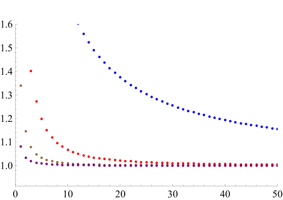
Figure 3: In this figure, we show the ratio $\displaystyle{\frac{4\pi}{k(-1)^{k+1}}\frac{a_{k}}{a_{k-1}}}$, where the $a_{k}$ are given by Eq.(76). The blue line represents the original coefficients, while the red, brown, and purple lines denote, respectively, the first three Richardson extrapolations.

$$\mathcal{B}\left[\frac{\Delta_{-1}}{Q^{3/2}}\right](t)=\sum_{k=0}^{\infty}\frac{a_{k}}{k!}t^{k}=\sum_{m=1}^{\infty}\frac{\left(i-1\right)}{\sqrt{2}\pi m^{3/2}}\left[\,{}_{2}F_{1}\left(-\frac{3}{2},\frac{5}{2};1;-\frac{it}{4m\pi}\right)+i\ _{2}F_{1}\left(-\frac{3}{2},\frac{5}{2};1;\frac{it}{4m\pi}\right)\right]\,.$$ (77)

Here $\,{}_{2}F_{1}(a,b;c;x)$ denotes the Hypergeometric function, which can be analytically continued in the complex plane along any path avoiding the branch points at $x=1$ and $x=\infty$. Hence $\mathcal{B}\left[\frac{\Delta_{-1}}{Q^{3/2}}\right](t)$ features an infinite series of branch points at $t=4\pi im$, $m\in\mathbb{Z}$, as shown in Fig.4.

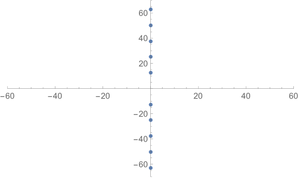
Figure 4: The singularity structure of the Borel transform of $\Delta_{-1}$ (77). There are branch points at $t=4\pi im$, $m\in\mathbb{Z}$.

As a consequence, the series (75) is Borel summable and both lateral Borel summations coincide

$$\Delta_{-1}=Q^{5/2}\int_{0}^{\infty}dt\ e^{-Qt}\mathcal{B}\left[\frac{\Delta_{-1}}{Q^{3/2}}\right](t)=\sum_{m=1}\frac{2iQ^{2}}{\pi m}\left[e^{x}K_{2}(x)-e^{-x}K_{2}(-x)\right]\,,\qquad x\equiv 2i\pi mQ\,,$$ (78)

where $K_{2}$ is the modified Bessel function of the second kind. Finally, the optimal truncation order corresponds to the value of $k$ such that $a_{k}/Q^{k}$ has a minimum and reads

$$k_{\text{opt}}\approx 4\pi Q\,,$$ (79)

with an error of order $\mathcal{O}\left(e^{-4\pi Q}\right)$. We conclude that, even if the $QED_{3}$ model shares the same universal large-charge behaviour (3) of the three-dimensional $O(N)$ model, its large-charge expansion behaves better than $O(N)$, having a higher optimal truncation order (i.e. $\approx Q$ rather than $\approx\sqrt{Q}$) and being Borel summable. Notice that, since at the leading order in $1/N_{f}$ the scaling dimensions are not affected by the inclusion of a Gross-Neveu interaction term, our results apply also to $QED_{3}-GN$ Dupuis:2021flq .

V CONCLUSIONS

In this work we studied the analytic structure of the fixed charge expansion for $O(N)$ in different space-time dimensions and $QED_{3}$. We have seen that in $d=3-\epsilon$ dimensions the contribution to the $O(N)$ fixed charge conformal dimensions, obtained in the double scaling limit of large charge and vanishing $\epsilon$, is non-Borel summable. Additionally, we have shown that the series is doubly factorial divergent and displays $\sqrt{Q}$ optimal truncation order. Resurgence technologies helped us show that the singularities in the Borel plane are connected to worldline instantons that were found in the alternative double scaling limit of large $Q$ and $N$ of Ref. Dondi:2021buw . We have also explored the case of $d=4-\epsilon$ and shown that in the same large $Q$ and small $\epsilon$ regime the next order corrections to the scaling dimensions amount to a convergent series. The resummed series exhibits a new branch cut singularity which we found to be relevant for the stability of the large charge sector of the $O(N)$ model for negative $\epsilon$. In the future, it would be interesting to include the contribution of radial and conformal modes to learn how they affect the analytic structure of the fixed charge expansion. For the $QED_{3}$ model we discovered that at leading order in the large number of matter field expansion the large charge scaling dimensions are Borel summable, single factorial divergent and with order $Q$ optimal truncation order. It would be also interesting to investigate whether a non-Borel summable expansion emerges at subleading $1/N_{f}$ orders ($\Delta_{0}$ has been computed in Pufu:2013vpa for $QED_{3}$ and in Dupuis:2021flq for $QED_{3}-GN$).

References

- (1) N. Dondi, I. Kalogerakis, D. Orlando and S. Reffert, “Resurgence of the large-charge expansion,” JHEP 05 (2021), 035 doi:10.1007/JHEP05(2021)035 [arXiv:2102.12488 [hep-th]].
- (2) J. L. Cardy, “Scaling and renormalization in statistical physics,” Cambridge, UK: Univ. Pr. 238 p. (Cambridge lecture notes in physics: 3), 1996.
- (3) M. Della Morte, D. Orlando and F. Sannino, “Renormalization Group Approach to Pandemics: The COVID-19 Case,” Front. in Phys. 8 (2020), 144 doi:10.3389/fphy.2020.00144
- (4) G. Cacciapaglia and F. Sannino, “Evidence for Complex Fixed Points in Pandemic Data” Front. Appl. Math. 7 (2021), p. 659580 doi:10.3389/fams.2021.659580
- (5) G. Cacciapaglia, C. Cot, A. De Hoffer, S. Hohennegger, F. Sannino, S. Vatani, “Epidemiological theory of virus variants” Accepted for publication in Physica A. [arXiv:2106.14982 [q-bio.PE]]
- (6) G. Cacciapaglia, C. Cot, and F. Sannino, “Second wave covid-19 pandemics in europe: A temporal playbook,” Sci Rep, vol. 10, p. 15514, 2020.
- (7) G. Cacciapaglia, C. Cot, M. Della Morte, S. Hohenegger, F. Sannino and S. Vatani, “The field theoretical ABC of epidemic dynamics,” [arXiv:2101.11399 [q-bio.PE]].
- (8) J. C. Le Guillou and J. Zinn-Justin, “Large order behavior of perturbation theory,”
- (9) L. N. Lipatov, “Divergence of the Perturbation Theory Series and the Quasiclassical Theory,” Sov. Phys. JETP 45 (1977), 216-223 LENINGRAD-76-255.
- (10) J. Ecalle, “Les Fonctions Resurgentes,” Prepub. Math. Universite Paris-Sud 81-05 (1981), 81-06 (1981), 85-05 (1985).
- (11) D. Dorigoni, “An Introduction to Resurgence, Trans-Series and Alien Calculus,” Annals Phys. 409 (2019), 167914 doi:10.1016/j.aop.2019.167914 [arXiv:1411.3585 [hep-th]].
- (12) I. Aniceto, G. Basar and R. Schiappa, “A Primer on Resurgent Transseries and Their Asymptotics,” Phys. Rept. 809 (2019), 1-135 doi:10.1016/j.physrep.2019.02.003 [arXiv:1802.10441 [hep-th]].
- (13) G. V. Dunne and M. Unsal, “Resurgence and Trans-series in Quantum Field Theory: The CP(N-1) Model,” JHEP 11 (2012), 170 doi:10.1007/JHEP11(2012)170 [arXiv:1210.2423 [hep-th]].
- (14) G. V. Dunne and M. Ünsal, “Continuity and Resurgence: towards a continuum definition of the (N-1) model,” Phys. Rev. D 87 (2013), 025015 doi:10.1103/PhysRevD.87.025015 [arXiv:1210.3646 [hep-th]].
- (15) P. Argyres and M. Unsal, “A semiclassical realization of infrared renormalons,” Phys. Rev. Lett. 109 (2012), 121601 doi:10.1103/PhysRevLett.109.121601 [arXiv:1204.1661 [hep-th]].
- (16) A. Cherman, D. Dorigoni and M. Unsal, “Decoding perturbation theory using resurgence: Stokes phenomena, new saddle points and Lefschetz thimbles,” JHEP 10 (2015), 056 doi:10.1007/JHEP10(2015)056 [arXiv:1403.1277 [hep-th]].
- (17) D. Dorigoni and Y. Hatsuda, “Resurgence of the Cusp Anomalous Dimension,” JHEP 09 (2015), 138 doi:10.1007/JHEP09(2015)138 [arXiv:1506.03763 [hep-th]].
- (18) A. Behtash, T. Sulejmanpasic, T. Schäfer and M. Ünsal, “Hidden topological angles and Lefschetz thimbles,” Phys. Rev. Lett. 115 (2015) no.4, 041601 doi:10.1103/PhysRevLett.115.041601 [arXiv:1502.06624 [hep-th]].
- (19) M. Yamazaki and K. Yonekura, “From 4d Yang-Mills to 2d model: IR problem and confinement at weak coupling,” JHEP 07 (2017), 088 doi:10.1007/JHEP07(2017)088 [arXiv:1704.05852 [hep-th]].
- (20) D. Boito, I. Caprini, M. Golterman, K. Maltman and S. Peris, “Hyperasymptotics and quark-hadron duality violations in QCD,” Phys. Rev. D 97 (2018) no.5, 054007 doi:10.1103/PhysRevD.97.054007 [arXiv:1711.10316 [hep-ph]].
- (21) K. Ishikawa, O. Morikawa, A. Nakayama, K. Shibata, H. Suzuki and H. Takaura, “Infrared renormalon in the supersymmetric model on ,” PTEP 2020 (2020) no.2, 023B10 doi:10.1093/ptep/ptaa002 [arXiv:1908.00373 [hep-th]].
- (22) M. Mariño and T. Reis, “Renormalons in integrable field theories,” JHEP 04 (2020), 160 doi:10.1007/JHEP04(2020)160 [arXiv:1909.12134 [hep-th]].
- (23) K. Ishikawa, O. Morikawa, K. Shibata, H. Suzuki and H. Takaura, “Renormalon structure in compactified spacetime,” PTEP 2020 (2020) no.1, 013B01 doi:10.1093/ptep/ptz147 [arXiv:1909.09579 [hep-th]].
- (24) J. Bersini, A. Maiezza and J. C. Vasquez, “Resurgence of the renormalization group equation,” Annals Phys. 415 (2020), 168126 doi:10.1016/j.aop.2020.168126 [arXiv:1910.14507 [hep-th]].
- (25) M. C. Abbott, Z. Bajnok, J. Balog, Á. Hegedús and S. Sadeghian, “Resurgence in the O(4) sigma model,” JHEP 05 (2021), 253 doi:10.1007/JHEP05(2021)253 [arXiv:2011.12254 [hep-th]].
- (26) M. Borinsky and G. V. Dunne, “Non-Perturbative Completion of Hopf-Algebraic Dyson-Schwinger Equations,” Nucl. Phys. B 957 (2020), 115096 doi:10.1016/j.nuclphysb.2020.115096 [arXiv:2005.04265 [hep-th]].
- (27) G. V. Dunne and Z. Harris, “Higher-loop Euler-Heisenberg transseries structure,” Phys. Rev. D 103 (2021) no.6, 065015 doi:10.1103/PhysRevD.103.065015 [arXiv:2101.10409 [hep-th]].
- (28) A. Maiezza and J. C. Vasquez, “Resurgence of the QCD Adler function,” Phys. Lett. B 817 (2021), 136338 doi:10.1016/j.physletb.2021.136338 [arXiv:2104.03095 [hep-ph]].
- (29) G. V. Dunne and M. Meynig, “Instantons or Renormalons? A Comment on Theory in the MS Scheme,” [arXiv:2111.15554 [hep-th]].
- (30) M. Marino, R. Miravitllas and T. Reis, “New renormalons from analytic trans-series,” [arXiv:2111.11951 [hep-th]]. LaTeX (EU)
- (31) P. C. Argyres and M. Unsal, “The semi-classical expansion and resurgence in gauge theories: new perturbative, instanton, bion, and renormalon effects,” JHEP 08 (2012), 063 doi:10.1007/JHEP08(2012)063 [arXiv:1206.1890 [hep-th]].
- (32) C. Pisani and E.R. Smith, “Lee-Yang Zeros and Stokes Phenomenon in a Model with a Wetting Transition,” J.Statist.Phys. 72 (1993) 51
- (33) T. Kanazawa and Y. Tanizaki, “Structure of Lefschetz thimbles in simple fermionic systems,” JHEP 03 (2015), 044 doi:10.1007/JHEP03(2015)044 [arXiv:1412.2802 [hep-th]].
- (34) P. V. Buividovich, G. V. Dunne and S. N. Valgushev, “Complex Path Integrals and Saddles in Two-Dimensional Gauge Theory,” Phys. Rev. Lett. 116 (2016) no.13, 132001 doi:10.1103/PhysRevLett.116.132001 [arXiv:1512.09021 [hep-th]].
- (35) A. Ahmed and G. V. Dunne, “Transmutation of a Trans-series: The Gross-Witten-Wadia Phase Transition,” JHEP 11 (2017), 054 doi:10.1007/JHEP11(2017)054 [arXiv:1710.01812 [hep-th]].
- (36) T. Fujimori, M. Honda, S. Kamata, T. Misumi, N. Sakai and T. Yoda, “Quantum phase transition and resurgence: Lessons from three-dimensional supersymmetric quantum electrodynamics,” PTEP 2021 (2021) no.10, 103B04 doi:10.1093/ptep/ptab086 [arXiv:2103.13654 [hep-th]].
- (37) G. Basar, G. Dunne and Z. Yin, “Uniformizing Lee-Yang Singularities,” [arXiv:2112.14269 [hep-th]].
- (38) S. Hellerman, D. Orlando, S. Reffert and M. Watanabe, “On the CFT Operator Spectrum at Large Global Charge,” JHEP 12 (2015), 071 doi:10.1007/JHEP12(2015)071 [arXiv:1505.01537 [hep-th]].
- (39) A. Monin, D. Pirtskhalava, R. Rattazzi and F. K. Seibold, “Semiclassics, Goldstone Bosons and CFT data,” JHEP 06 (2017), 011 doi:10.1007/JHEP06(2017)011 [arXiv:1611.02912 [hep-th]].
- (40) L. Alvarez-Gaume, O. Loukas, D. Orlando and S. Reffert, “Compensating strong coupling with large charge,” JHEP 04 (2017), 059 doi:10.1007/JHEP04(2017)059 [arXiv:1610.04495 [hep-th]].
- (41) D. Banerjee, S. Chandrasekharan and D. Orlando, “Conformal dimensions via large charge expansion,” Phys. Rev. Lett. 120 (2018) no.6, 061603 doi:10.1103/PhysRevLett.120.061603 [arXiv:1707.00711 [hep-lat]].
- (42) S. Hellerman and S. Maeda, “On the Large -charge Expansion in Superconformal Field Theories,” JHEP 12 (2017), 135 doi:10.1007/JHEP12(2017)135 [arXiv:1710.07336 [hep-th]].
- (43) A. De La Fuente, “The large charge expansion at large ,” JHEP 08 (2018), 041 doi:10.1007/JHEP08(2018)041 [arXiv:1805.00501 [hep-th]].
- (44) D. Orlando, S. Reffert and F. Sannino, “A safe CFT at large charge,” JHEP 08 (2019), 164 doi:10.1007/JHEP08(2019)164 [arXiv:1905.00026 [hep-th]].
- (45) D. Banerjee, S. Chandrasekharan, D. Orlando and S. Reffert, “Conformal dimensions in the large charge sectors at the O(4) Wilson-Fisher fixed point,” Phys. Rev. Lett. 123 (2019) no.5, 051603 doi:10.1103/PhysRevLett.123.051603 [arXiv:1902.09542 [hep-lat]].
- (46) G. Cuomo, “A note on the large charge expansion in 4d CFT,” Phys. Lett. B 812 (2021), 136014 doi:10.1016/j.physletb.2020.136014 [arXiv:2010.00407 [hep-th]].
- (47) S. Hellerman and D. Orlando, “Large R-charge EFT correlators in N=2 SQCD,” [arXiv:2103.05642 [hep-th]].
- (48) G. Cuomo, “OPE meets semiclassics,” Phys. Rev. D 103 (2021) no.8, 085005 doi:10.1103/PhysRevD.103.085005 [arXiv:2103.01331 [hep-th]].
- (49) G. Cuomo, M. Mezei and A. Raviv-Moshe, “Boundary conformal field theory at large charge,” JHEP 10 (2021), 143 doi:10.1007/JHEP10(2021)143 [arXiv:2108.06579 [hep-th]].
- (50) V. Pellizzani, “Operator spectrum of nonrelativistic CFTs at large charge,” [arXiv:2107.12127 [hep-th]].
- (51) S. Hellerman, D. Orlando, V. Pellizzani, S. Reffert and I. Swanson, “Nonrelativistic CFTs at Large Charge: Casimir Energy and Logarithmic Enhancements,” [arXiv:2111.12094 [hep-th]].
- (52) D. Banerjee and S. Chandrasekharan, “Sub-leading conformal dimensions at the O(4) Wilson-Fisher fixed point,” [arXiv:2111.01202 [hep-lat]].
- (53) L. Alvarez-Gaume, D. Orlando and S. Reffert, “Large charge at large N,” JHEP 12 (2019), 142 doi:10.1007/JHEP12(2019)142 [arXiv:1909.02571 [hep-th]].
- (54) G. Badel, G. Cuomo, A. Monin and R. Rattazzi, “The Epsilon Expansion Meets Semiclassics,” JHEP 11 (2019), 110 doi:10.1007/JHEP11(2019)110 [arXiv:1909.01269 [hep-th]].
- (55) G. Badel, G. Cuomo, A. Monin and R. Rattazzi, “Feynman diagrams and the large charge expansion in dimensions,” Phys. Lett. B 802 (2020), 135202 doi:10.1016/j.physletb.2020.135202 [arXiv:1911.08505 [hep-th]].
- (56) O. Antipin, J. Bersini, F. Sannino, Z. W. Wang and C. Zhang, “Charging the model,” Phys. Rev. D 102 (2020) no.4, 045011 doi:10.1103/PhysRevD.102.045011 [arXiv:2003.13121 [hep-th]].
- (57) O. Antipin, J. Bersini, F. Sannino, Z. W. Wang and C. Zhang, “Charging non-Abelian Higgs theories,” Phys. Rev. D 102 (2020) no.12, 125033 doi:10.1103/PhysRevD.102.125033 [arXiv:2006.10078 [hep-th]].
- (58) O. Antipin, J. Bersini, F. Sannino, Z. W. Wang and C. Zhang, “Untangling scaling dimensions of fixed charge operators in Higgs theories,” Phys. Rev. D 103 (2021) no.12, 125024 doi:10.1103/PhysRevD.103.125024 [arXiv:2102.04390 [hep-th]].
- (59) O. Antipin, J. Bersini, F. Sannino, Z. W. Wang and C. Zhang, “More on the cubic versus quartic interaction equivalence in the model,” Phys. Rev. D 104 (2021), 085002 doi:10.1103/PhysRevD.104.085002 [arXiv:2107.02528 [hep-th]].
- (60) G. Arias-Tamargo, D. Rodriguez-Gomez and J. G. Russo, “The large charge limit of scalar field theories and the Wilson-Fisher fixed point at ,” JHEP 10 (2019), 201 doi:10.1007/JHEP10(2019)201 [arXiv:1908.11347 [hep-th]].
- (61) G. Arias-Tamargo, D. Rodriguez-Gomez and J. G. Russo, “On the UV completion of the model in dimensions: a stable large-charge sector,” [arXiv:2003.13772 [hep-th]].
- (62) I. Jack and D. R. T. Jones, “Anomalous dimensions for in scale invariant theory,” Phys. Rev. D 102 (2020) no.8, 085012 doi:10.1103/PhysRevD.102.085012 [arXiv:2007.07190 [hep-th]].
- (63) I. Jack and D. R. T. Jones, “Anomalous dimensions at large charge in d=4 O(N) theory,” Phys. Rev. D 103 (2021) no.8, 085013 doi:10.1103/PhysRevD.103.085013 [arXiv:2101.09820 [hep-th]].
- (64) I. Jack and D. R. T. Jones, “Anomalous dimensions at large charge for U(N)×U(N) theory in three and four dimensions,” Phys. Rev. D 104 (2021) no.10, 105017 doi:10.1103/PhysRevD.104.105017 [arXiv:2108.11161 [hep-th]].
- (65) I. Jack and D. R. T. Jones, “Scaling dimensions at large charge for cubic theory in six dimensions,” [arXiv:2112.01196 [hep-th]].
- (66) S. Giombi and J. Hyman, “On the Large Charge Sector in the Critical Model at Large ,” [arXiv:2011.11622 [hep-th]].
- (67) S. Giombi, S. Komatsu and B. Offertaler, “Large Charges on the Wilson Loop in SYM: Matrix Model and Classical String,” [arXiv:2110.13126 [hep-th]].
- (68) T. Araujo, O. Celikbas, D. Orlando and S. Reffert, “2D CFTs – Large Charge is not enough,” [arXiv:2112.03286 [hep-th]].
- (69) D. Rodriguez-Gomez, “A Scaling Limit for Line and Surface Defects,” [arXiv:2202.03471 [hep-th]].
- (70) D. T. Son, “Semiclassical approach for multiparticle production in scalar theories,” Nucl. Phys. B 477 (1996), 378-406 doi:10.1016/0550-3213(96)00386-0 [arXiv:hep-ph/9505338 [hep-ph]].
- (71) D. Orlando, S. Reffert and F. Sannino, “Near-Conformal Dynamics at Large Charge,” Phys. Rev. D 101 (2020) no.6, 065018 doi:10.1103/PhysRevD.101.065018 [arXiv:1909.08642 [hep-th]].
- (72) D. Orlando, S. Reffert and F. Sannino, “Charging the Conformal Window,” Phys. Rev. D 103 (2021) no.10, 105026 doi:10.1103/PhysRevD.103.105026 [arXiv:2003.08396 [hep-th]].
- (73) D. Orlando, S. Reffert and T. Schmidt, “Following the flow for large N and large charge,” [arXiv:2110.07616 [hep-th]].
- (74) R. Moser, D. Orlando and S. Reffert, “Convexity, large charge and the large-N phase diagram of the theory,” [arXiv:2110.07617 [hep-th]].
- (75) S. Hellerman, “On the exponentially small corrections to superconformal correlators at large R-charge,” [arXiv:2103.09312 [hep-th]].
- (76) M. Moshe and J. Zinn-Justin, “Quantum field theory in the large N limit: A Review,” Phys. Rept. 385 (2003), 69-228 doi:10.1016/S0370-1573(03)00263-1 [arXiv:hep-th/0306133 [hep-th]].
- (77) J. L. Cardy, “Conformal invariance and universality in finite-size scaling,” J. Phys. A 17, L385 (1984).
- (78) J. L. Cardy, “Universal amplitudes in finite-size scaling: generalisation to arbitrary dimensionality,” J. Phys. A 18 (1985) no.13, L757. doi:10.1088/0305-4470/18/13/005
- (79) L. Di Pietro, M. Mariño, G. Sberveglieri and M. Serone, “Resurgence and 1/N Expansion in Integrable Field Theories,” JHEP 10 (2021), 166 doi:10.1007/JHEP10(2021)166 [arXiv:2108.02647 [hep-th]].
- (80) C. Schubert, “Perturbative quantum field theory in the string inspired formalism,” Phys. Rept. 355 (2001), 73-234 doi:10.1016/S0370-1573(01)00013-8 [arXiv:hep-th/0101036 [hep-th]].
- (81) A. J. Guttmann, J.Phys.A 49 (2016) 415002 • DOI: 10.1088/1751-8113/49/41/415002
- (82) M. E. Fisher, Rocky Mt.J.Math. 4 (1974) 181 • DOI:10.1216/RMJ-1974-4-2-181
- (83) I. Caprini, J. Fischer, G. Abbas and B. Ananthanarayan, “Perturbative Expansions in QCD Improved by Conformal Mappings of the Borel Plane,” [arXiv:1711.04445 [hep-ph]].
- (84) W. R. Frazer, “Applications of Conformal Mapping to the Phenomenological Representation of Scattering Amplitudes,” Phys. Rev. 123 (1961), 2180-2182 doi:10.1103/PhysRev.123.2180
- (85) D. L. Hunter and G. A. Baker, “Methods of Series Analysis. 1. Comparison of Current Methods Used in the Theory of Critical Phenomena,” Phys. Rev. B 7 (1973), 3346-3376 doi:10.1103/PhysRevB.7.3346
- (86) D. I. Kazakov, D. V. Shirkov and O. V. Tarasov, “Analytical Continuation of Perturbative Results of the Model Into the Region Is Greater Than or Equal to 1,” Theor. Math. Phys. 38 (1979), 9-16 doi:10.1007/BF01030252
- (87) N. A. Dondi, G. V. Dunne, M. Reichert and F. Sannino, “Analytic Coupling Structure of Large (Super) QED and QCD,” Phys. Rev. D 100 (2019) no.1, 015013 doi:10.1103/PhysRevD.100.015013 [arXiv:1903.02568 [hep-th]].
- (88) N. A. Dondi, G. V. Dunne, M. Reichert and F. Sannino, “Towards the QED beta function and renormalons at and ,” Phys. Rev. D 102 (2020) no.3, 035005 doi:10.1103/PhysRevD.102.035005 [arXiv:2003.08397 [hep-th]].
- (89) O. Costin and G. V. Dunne, “Physical Resurgent Extrapolation,” Phys. Lett. B 808 (2020), 135627 doi:10.1016/j.physletb.2020.135627 [arXiv:2003.07451 [hep-th]].
- (90) J. Fischer, “On the role of power expansions in quantum field theory,” Int. J. Mod. Phys. A 12 (1997), 3625-3663 doi:10.1142/S0217751X97001870 [arXiv:hep-ph/9704351 [hep-ph]].
- (91) M. A. Stephanov, “QCD critical point and complex chemical potential singularities,” Phys. Rev. D 73 (2006), 094508 doi:10.1103/PhysRevD.73.094508 [arXiv:hep-lat/0603014 [hep-lat]].
- (92) S. Giombi, I. R. Klebanov and B. R. Safdi, “Higher Spin AdSd+1/CFTd at One Loop,” Phys. Rev. D 89 (2014) no.8, 084004 doi:10.1103/PhysRevD.89.084004 [arXiv:1401.0825 [hep-th]].
- (93) R. Camporesi, “Harmonic analysis and propagators on homogeneous spaces,” Phys. Rept. 196 (1990), 1-134 doi:10.1016/0370-1573(90)90120-Q
- (94) A. N. Redlich, “Gauge Noninvariance and Parity Violation of Three-Dimensional Fermions,” Phys. Rev. Lett. 52 (1984), 18 doi:10.1103/PhysRevLett.52.18
- (95) R. D. Pisarski, “Chiral Symmetry Breaking in Three-Dimensional Electrodynamics,” Phys. Rev. D 29 (1984), 2423 doi:10.1103/PhysRevD.29.2423
- (96) T. Appelquist, D. Nash and L. C. R. Wijewardhana, “Critical Behavior in (2+1)-Dimensional QED,” Phys. Rev. Lett. 60 (1988), 2575 doi:10.1103/PhysRevLett.60.2575
- (97) D. Nash, “Higher Order Corrections in (2+1)-Dimensional QED,” Phys. Rev. Lett. 62 (1989), 3024 doi:10.1103/PhysRevLett.62.3024
- (98) V. Borokhov, A. Kapustin and X. k. Wu, “Topological disorder operators in three-dimensional conformal field theory,” JHEP 11 (2002), 049 doi:10.1088/1126-6708/2002/11/049 [arXiv:hep-th/0206054 [hep-th]].
- (99) P. Maris, “Confinement and complex singularities in QED in three-dimensions,” Phys. Rev. D 52 (1995), 6087-6097 doi:10.1103/PhysRevD.52.6087 [arXiv:hep-ph/9508323 [hep-ph]].
- (100) J. Braun, H. Gies, L. Janssen and D. Roscher, “Phase structure of many-flavor QED3,” Phys. Rev. D 90 (2014) no.3, 036002 doi:10.1103/PhysRevD.90.036002 [arXiv:1404.1362 [hep-ph]].
- (101) S. Giombi, I. R. Klebanov and G. Tarnopolsky, “Conformal QEDd, -Theorem and the Expansion,” J. Phys. A 49 (2016) no.13, 135403 doi:10.1088/1751-8113/49/13/135403 [arXiv:1508.06354 [hep-th]].
- (102) S. M. Chester and S. S. Pufu, “Towards bootstrapping QED3,” JHEP 08 (2016), 019 doi:10.1007/JHEP08(2016)019 [arXiv:1601.03476 [hep-th]].
- (103) S. Albayrak, R. S. Erramilli, Z. Li, D. Poland and Y. Xin, “Bootstrapping conformal QED3,” [arXiv:2112.02106 [hep-th]].
- (104) S. S. Pufu, “Anomalous dimensions of monopole operators in three-dimensional quantum electrodynamics,” Phys. Rev. D 89 (2014) no.6, 065016 doi:10.1103/PhysRevD.89.065016 [arXiv:1303.6125 [hep-th]].
- (105) V. P. Gusynin and P. K. Pyatkovskiy, “Critical number of fermions in three-dimensional QED,” Phys. Rev. D 94 (2016) no.12, 125009 doi:10.1103/PhysRevD.94.125009 [arXiv:1607.08582 [hep-ph]].
- (106) W. Rantner and X. G. Wen, “Spin correlations in the algebraic spin liquid: Implications for high-Tc superconductors,” Phys. Rev. B 66 (2002), 144501 doi:10.1103/PhysRevB.66.144501 [arXiv:cond-mat/0201521 [cond-mat.str-el]].
- (107) A. M. Polyakov, “Compact Gauge Fields and the Infrared Catastrophe,” Phys. Lett. B 59 (1975), 82-84 doi:10.1016/0370-2693(75)90162-8
- (108) A. M. Polyakov, “Quark Confinement and Topology of Gauge Groups,” Nucl. Phys. B 120 (1977), 429-458 doi:10.1016/0550-3213(77)90086-4
- (109) T. T. Wu and C. N. Yang, “Dirac Monopole Without Strings: Monopole Harmonics,” Nucl. Phys. B 107 (1976), 365 doi:10.1016/0550-3213(76)90143-7
- (110) T. T. Wu and C. N. Yang, “Some Properties of Monopole Harmonics,” Phys. Rev. D 16 (1977), 1018-1021 doi:10.1103/PhysRevD.16.1018
- (111) É. Dupuis, R. Boyack and W. Witczak-Krempa, “Anomalous dimensions of monopole operators at the transitions between Dirac and topological spin liquids,” [arXiv:2108.05922 [cond-mat.str-el]].
- (112) Y. C. He, D. N. Sheng and Y. Chen, “Chiral Spin Liquid in a Frustrated Anisotropic Kagome Heisenberg Model,” Phys. Rev. Lett. 112 (2014) no.13, 137202 doi:10.1103/PhysRevLett.112.137202 [arXiv:1312.3461 [cond-mat.str-el]].
- (113) Y. C. He, Y. Fuji and S. Bhattacharjee, “Kagome spin liquid: a deconfined critical phase driven by gauge fluctuation,” [arXiv:1512.05381 [cond-mat.str-el]].
- (114) L. Janssen and Y. C. He, “Critical behavior of the QED3-Gross-Neveu model: Duality and deconfined criticality,” Phys. Rev. B 96 (2017) no.20, 205113 doi:10.1103/PhysRevB.96.205113 [arXiv:1708.02256 [cond-mat.str-el]].
- (115) R. D. Pisarski, “FIXED POINT STRUCTURE OF (PHI**6) in three-dimensions AT LARGE N,” Phys. Rev. Lett. 48 (1982), 574-576 doi:10.1103/PhysRevLett.48.574
- (116) J. D. Brock, A. Aharony, R. J. Birgeneau, K. W. Evans-Lutterodt, J. D. Litster, P. M. Horn, G. B. Stephenson, and A. R. Tajbakhsh, “Orientational and positional order in a tilted hexatic liquid-crystal phase,” Phys. Rev. Lett. 57, 98 (1985).
- (117) A. Aharony, in Phase Transitions and Critical Phenomena, edited by C. Domb and J. Lebowitz (Academic Press, New York, 1976), Vol. 6, p. 357.
- (118) S. C. Zhang, “A Unified Theory Based on SO(5) Symmetry of Superconductivity and Antiferromagnetism,” Science 275, 1089-1097 (1997), DOI: 10.1126/science.275.5303.1089
- (119) C. M. Bender and S. A. Orszag, “Advanced Mathematical Methods for Scientists and Engineers,” (Springer, 1999)
- (120) D. Shanks, “Non-linear transformations of divergent and slowly convergent sequences,” Journal of Mathematics and Physics 34.1-4 (1955), pp. 1–42.