Statistically Efficient Advantage Learning for Offline Reinforcement Learning in Infinite Horizons

Abstract

We consider reinforcement learning (RL) methods in offline domains without additional online data collection, such as mobile health applications. Most of existing policy optimization algorithms in the computer science literature are developed in online settings where data are easy to collect or simulate. Their generalizations to mobile health applications with a pre-collected offline dataset remain unknown. The aim of this paper is to develop a novel advantage learning framework in order to efficiently use pre-collected data for policy optimization. The proposed method takes an optimal Q-estimator computed by any existing state-of-the-art RL algorithms as input, and outputs a new policy whose value is guaranteed to converge at a faster rate than the policy derived based on the initial Q-estimator. Extensive numerical experiments are conducted to back up our theoretical findings. A Python implementation of our proposed method is available at https://github.com/leyuanheart/SEAL.

Keywords: Reinforcement learning; Advantage learning; Infinite horizons; Rate of convergence; Mobile health applications.

1 Introduction

Reinforcement learning (RL, see Sutton and Barto, 2018, for an overview) is concerned with how intelligence agents learn and take actions in an unknown environment in order to maximize the cumulative reward that it receives. It has been arguably one of the most vibrant research frontiers in machine learning over the last few years. According to Google Scholar, over 40K scientific articles have been published in 2020 with the phrase “reinforcement learning”. Over 100 papers on RL were accepted for presentation at ICML 2021, a premier conference in the machine learning area, accounting for more than 10% of the accepted papers in total. RL algorithms have been applied in a wide variety of real applications, including games (Silver et al., 2016), robotics (Kormushev et al., 2013), healthcare (Komorowski et al., 2018), bidding (Jin et al., 2018), ridesharing (Xu et al., 2018) and automated driving (de Haan et al., 2019), to name a few.

This paper is partly motivated by developing statistical learning methodologies in offline RL domains such as mobile health (mHealth). mHealth technologies have recently emerged due to the use of mobile phones, tablets computers or wearable devices. They play an important role in precision medicine as they offer a means to monitor a patient’s health status and deliver interventions in real-time. They also collect rich longitudinal data for optimal treatment decision making. One motivating example being considered in this paper uses the OhioT1DM Dataset (Marling and Bunescu, 2018). It contains 8 weeks of data for 6 patients with type 1 diabetes, an autoimmune disease wherein the pancreas produces insufficient levels of insulin. For those patients, their continuous glucose monitoring blood glucose levels, insulin doses being injected, self-reported times of meals and exercises are continually measured. Their outcomes have the potential to be improved by treatment policies tailored to the continually evolving health status of each patient (Luckett et al., 2020; Shi et al., 2020).

Despite the popularity of developing various RL algorithms in the computer science literature, statistics as a field, has only recently begun to engage with RL both in depth and in breadth. Most works in the statistics literature focused on developing data-driven methodologies for precision medicine with only a few treatment stages (see e.g., Murphy, 2003; Robins, 2004; Chakraborty et al., 2010; Qian and Murphy, 2011; Zhang et al., 2013; Zhao et al., 2015; Wallace and Moodie, 2015; Song et al., 2015; Luedtke and van der Laan, 2016; Zhang et al., 2018; Zhu et al., 2017; Shi et al., 2018; Wang et al., 2018; Qi et al., 2020; Nie et al., 2020). These methods require a large number of patients in the observed data to be consistent. They are not applicable to mHealth applications with only a few patients, which is the case in the OhioT1DM dataset. Nor are they applicable to many other sequential decision making problems in infinite horizons where the number of decision stages is allowed to diverge to infinity, such as games or robotics. Recently, a few algorithms have been proposed in the statistics literature for policy optimization in mHealth applications (Ertefaie and Strawderman, 2018; Luckett et al., 2020; Hu et al., 2020; Liao et al., 2020; Zhou et al., 2021).

Among all existing methods in infinite horizons, Q-learning (Watkins and Dayan, 1992) is arguably one of the most popular model-free RL algorithms. It derives the optimal policy by learning an optimal Q-function, without explicitly modelling the system dynamics. Variants of Q-learning include gradient Q-learning (Maei et al., 2010; Ertefaie and Strawderman, 2018), fitted Q-iteration (Riedmiller, 2005), deep Q-network (DQN, Mnih et al., 2015), double DQN (Van Hasselt et al., 2016) and quantile DQN (Dabney et al., 2018), among others. All these Q-learning type algorithms are primarily motivated by the application of developing artificial intelligence in online video games, so their generalization to offline applications with a pre-collected dataset remains unknown.

Different from online settings (e.g., video games) where data are easy to collect or simulate, the number of observations in many offline applications (e.g., healthcare) is limited. Take the OhioT1DM dataset as an example, only a few thousands observations are available (Shi et al., 2020). With such limited data, it is critical to develop RL algorithms that are statistically efficient. Instead of proposing a specific algorithm for policy optimization, our work undertakes the ambitious task of devising an “efficiency enhancement” method that is generally applicable to any Q-learning type algorithms to improve their statistical efficiency. The input of our method is an optimal Q-estimator computed by existing state-of-the-art RL algorithms and the output is a new policy whose value converges at a faster rate than the policy derived based on the initial Q-estimator.

The proposed method is motivated by a line of research on developing A-learning type algorithms to learn an optimal dynamic treatment regime (DTR) to implement precision medicine (see e.g., Murphy, 2003; Robins, 2004; Lu et al., 2013). These methods directly model the difference between two conditional mean functions (known as the contrast function). They are semi-parametrically efficient and outperform Q-learning (see e.g., Chakraborty et al., 2010; Qian and Murphy, 2011) in cases where the Q-function is misspecified (Shi et al., 2018). In addition, A-learning has the so-called doubly robustness property, i.e., the estimated optimal DTR is consistent when either the model for the conditional mean function or the treatment assignment mechanism is correctly specified.

The contributions of our paper are summarized as follows. Methodologically, we propose a statistically efficient advantage learning procedure to estimate the optimal policy in offline infinite horizon settings. Our proposal integrates existing policy optimization and policy evaluation algorithms in RL. Specifically, we start with applying existing Q-learning type algorithms to compute an initial estimator for the optimal Q-function. Based on these Q-estimators, we leverage ideas from the off-policy evaluation literature (OPE, see e.g. Jiang and Li, 2016; Thomas and Brunskill, 2016; Liu et al., 2018; Kallus and Uehara, 2019, 2020; Shi et al., 2021) to construct pseudo outcomes that are asymptotically unbiased to the optimal contrast function (see Section 2.2 for the detailed definition). With these pseudo outcomes as the prediction target, we can directly apply existing state-of-the-art supervised learning algorithms to derive the optimal policy. The use of OPE effectively alleviates the bias of the estimated contrast function resulting from the potential model misspecification of the optimal Q-function, which in turn improves the statistical efficiency over Q-learning. In that sense, our proposal shares similar spirits with the A-learning type methods to learn DTRs in finite horizons.

Theoretically, we show our estimated contrast function converges at a faster rate than the Q-function computed by existing state-of-the-art Q-learning type algorithms (Theorem 2). This in turn implies that our estimated policy achieves a larger value function (Theorem 3). All the error bounds derived in this paper converge to zero when either the number of trajectories $N$ or the number of decision stages per trajectory $T$ to approach infinity. This guarantees the consistency of our method when applied to a wide range of real-world problems, ranging from the OhioT1DM Dataset that contains eight weeks’ data for 6 patients to the 2018 Intern Health Study with over 1000 subjects (see e.g., NeCamp et al., 2020). It is also applicable to data generated from online video games where both $N$ and $T$ are allowed to grow to infinity.

Empirically, we show that our procedure outperforms existing learning algorithms using both synthetic datasets and a real dataset from the mobile health application. We remark that most papers in the existing literature use synthetic datasets to evaluate the performance of different RL algorithms. Results in our paper offer a useful evaluation tool for assessing these algorithms in real applications.

The rest of this article is organised as follows. In Section 2, we introduce some basic concepts in RL, describe the data generating process and formulate the problem. In Section 3, we demonstrate the advantage of A-learning over Q-learning by comparing their rate of convergence. The proposed algorithm is formally presented in Section 4. In Section 5, we study the statistical properties of our algorithm, proving that our estimated policy achieves a faster rate of convergence than existing Q-learning type algorithms. In Section 6, we investigate the finite sample performance of the proposed algorithm using Monte Carlo simulations. In Section 7, we use the OhioT1DM Dataset to further demonstrate the empirical advantage of the proposed algorithm over other baseline algorithms. Finally, we conclude our paper by a discussion section. Proofs of our major theorems are presented in Section A of the supplementary article.

2 Preliminaries

We first formulate the policy optimization problem in infinite horizon settings. We next briefly review Q-learning.

2.1 Problem Formulation

RL is concerned with solving sequential decision making problems in an unknown environment. The observed data can be summarized into a sequence of state-action-reward triplets over time. At each time $t\geq 0$, the decision maker observes some features from the environment, summarized into a state vector $S_{t}\in\mathbb{S}$ where the state space $\mathbb{S}$ is assumed to be a subset of $\mathbb{R}^{d}$. The decision maker then selects an action $A_{t}$ from the action space $\mathbb{A}$. The environment responds by providing the decision maker with an immediate reward $R_{t}\in\mathbb{R}$ and moving to the next state $S_{t+1}$. In this paper, we focus on the setting where $\mathbb{A}$ is discrete. Extensions to the continuous action space are discussed in Sections 8.1 and 8.2. The state space $\mathbb{S}$ can be either continuous or discrete.

A policy defines the agent’s way of behaving. A history-dependent policy $\pi$ is a sequence of decision rules $\{\pi_{t}\}_{t\geq 0}$ where each $\pi_{t}$ is a function that maps the observed data history to a probability distribution function on the action space at time $t$. When these decision rules are time-homogeneous (i.e., $\pi_{1}=\pi_{2}=\cdots=\pi_{t}=\cdots$) and depend on the past data history only through the current state vector, the resulting policy is referred to as a stationary policy. Following $\pi$, the discounted cumulative reward that the decision maker receives is referred to as the value function,

$$V^{\pi}(s)=\sum_{t=0}^{+\infty}\gamma^{t}{\mbox{E}}^{\pi}(R_{t}|S_{0}=s),$$

where the expectation ${\mbox{E}}^{\pi}$ is taken by assuming that actions are assigned according to $\pi$ and $0\leq\gamma<1$ is a discounted factor that balances the long-term and short-term rewards. The objective of policy optimization is to identify an optimal policy $\pi^{\tiny{opt}}$ that maximizes the value, i.e., $\pi^{\tiny{opt}}=\operatorname*{arg\,max}_{\pi}{\mbox{E}}V^{\pi}(S_{0})$.

We model the data generating process by a Markov decision process (MDP, Puterman, 1994). Specifically, we impose the following Markov assumption (MA) and conditional mean independence assumption (CMIA).

(MA) There exists some function $q$ such that for any $t\geq 0$, $\mathcal{S}\in\mathbb{S}$, we have

$${\mbox{Pr}}(S_{t+1}\in\mathcal{S}|\{S_{j},A_{j},R_{j}\}_{0\leq j\leq t})=\int_{\mathcal{S}}q(s;A_{t},S_{t})ds.$$

(CMIA) There exists some reward function $r$ such that for any $t\geq 0$, we have

$${\mbox{E}}(R_{t}|S_{t},A_{t},\{S_{j},A_{j},R_{j}\}_{0\leq j<t})=r(A_{t},S_{t}).$$

We make a few remarks. First, MA requires the future state to be conditional independent of the past data history given the current state-action pair. The function $q$ corresponds to the Markov transition density function that characterizes the state transitions. This assumption is testable from the observed data (see e.g., Shi et al., 2020). Second, under MA, CMIA is automatically satisfied when $R_{t}$ is a deterministic function of $S_{t},A_{t}$ and $S_{t+1}$. The latter assumption is commonly imposed in the literature (Ertefaie and Strawderman, 2018; Luckett et al., 2020). CMIA is weaker than this assumption.

Second, these two assumptions lay the foundations of the existing state-of-the-art RL algorithms (e.g., DQN). Specifically, they guarantee the existence of an optimal stationary policy that is no worse than any history-dependent policies (see e.g., Puterman, 1994). It allows us to restrict our attentions to the class of stationary policies. For any such policy $\pi$, we use $\pi(\bullet|s)$ to denote the probability mass function that the decision maker will follow to select actions given that the environment is in the state $s$.

The observed data consist of $N$ trajectories. Specifically, let $\{(S_{i,t},A_{i,t},R_{i,t},S_{i,t+1})\}_{0\leq t<T}$ be the data collected from the $i$-th trajectory where $T$ is the termination time. We assume these trajectories are independent copies of $\{(S_{t},A_{t},R_{t})\}_{t\geq 0}$. Our objective is to learn $\pi^{\scriptsize{opt}}$ based on this offline dataset.

2.2 Q-learning

For a given policy $\pi$, we define the state-action value function (better known as the Q-function) under $\pi$ as

$$Q^{\pi}(a,s)=\sum_{t\geq 0}\gamma^{t}{\mbox{E}}^{\pi}(R_{t}|A_{0}=a,S_{0}=s).$$

It represents the average cumulative reward that the decision maker will receive if they select the action $a$ initially and follow $\pi$ afterwards. In addition, notice that

$$\begin{split}Q^{\pi}(a,s)={\mbox{E}}(R_{0}|A_{0}=a,S_{0}=s)+\gamma\left\{\sum_{t\geq 0}\gamma^{t}{\mbox{E}}^{\pi}(R_{t+1}|A_{0}=a,S_{0}=s)\right\}\\ =r(a,s)+\gamma\left\{\sum_{t\geq 0}\gamma^{t}{\mbox{E}}^{\pi}[{\mbox{E}}^{\pi}(R_{t+1}|A_{1},S_{1},A_{0}=a,S_{0}=s)|A_{0},S_{0}]\right\}\\ =r(a,s)+\gamma{\mbox{E}}^{\pi}\{Q^{\pi}(A_{1},S_{1})|A_{0}=a,S_{0}=s\}\\ =r(a,s)+\gamma\int_{s^{\prime}}\sum_{a^{\prime}}\pi(a^{\prime}|s^{\prime})Q(a^{\prime},s^{\prime})q(s^{\prime};a,s)ds^{\prime},\end{split}$$ (1)

where the third equation follows from CMIA and the definition of $Q^{\pi}$ and the last equation follows from MA. The above equation is referred to as the Bellman equation for $Q^{\pi}$.

Define optimal Q-function $Q^{\tiny{opt}}$ as $Q^{\tiny{opt}}(a,s)=\max_{\pi}Q^{\pi}(a,s)$ for any state-action pair $(a,s)$. Under MA and CMIA, it can be shown that $\pi^{\scriptsize{opt}}$ satisfies

$$\pi^{\scriptsize{opt}}(a|s)=\mathbb{I}\left\{a=\operatorname*{arg\,max}_{a^{\prime}}Q^{\tiny{opt}}(a^{\prime},s)\right\},\,\,\,\forall a,s,$$ (2)

where $\mathbb{I}\{\cdot\}$ denotes the indicator function. In addition, we have $Q^{\tiny{opt}}=Q^{\pi^{\tiny{opt}}}$. Similar to (1), one can show that $Q^{\tiny{opt}}$ satisfies the following Bellman optimality equation,

$$Q^{\tiny{opt}}(a,s)=r(a,s)+\gamma\int_{s^{\prime}}\max_{a^{\prime}}Q^{\tiny{opt}}(s^{\prime},a^{\prime})q(s^{\prime};a,s)ds^{\prime},$$ (3)

or equivalently,

$$Q^{\tiny{opt}}(A_{t},S_{t})={\mbox{E}}\left\{R_{t}+\gamma\max_{a}Q^{\tiny{opt}}(a,S_{t+1})|A_{t},S_{t}\right\}.$$ (4)

Equations (2) and (4) form the basis for all Q-learning type algorithms. Specifically, these algorithms first estimate the optimal Q-function by solving (4) and then derive the estimated optimal policy based on (2). Take the fitted Q-iteration algorithm as an example. It iteratively updates the optimal Q-function using supervised learning. At each iteration, the input includes $(A_{t},S_{t})$ that serves as the “predictors” and $R_{t}+\gamma\max_{a}\widetilde{Q}(a,S_{t+1})$ that serves as the “response” where $\widetilde{Q}$ denotes the current estimate of the optimal Q-function.

Finally, we introduce the contrast function. For a given $\pi$, define the contrast function associated with $\pi$ as $\tau^{\pi}(a,s)=Q^{\pi}(a,s)-Q^{\pi}(a_{0},s)$ for some $a_{0}\in\mathbb{A}$. In practice, the control arm $a_{0}$ could be set to the action that occurs the most in the data. This is because the baseline Q-function $Q^{\pi}(a_{0},s)$ needs to be accurately estimated in order to consistently estimate the contrast function. Hence, it is natural to consider the most frequently selected arm, which has the largest number of observations to learn the baseline Q-function. Let $\tau^{\tiny{opt}}(a,s)=\tau^{\pi^{\tiny{opt}}}(a,s)$ be the optimal contrast function. Similar to (2), we obtain that

$$\pi^{\scriptsize{opt}}(a|s)=\mathbb{I}\{a=\operatorname*{arg\,max}_{a^{\prime}}\tau^{\tiny{opt}}(a^{\prime},s)\},$$

for any $a$ and $s$. Consequently, to estimate the optimal policy, it suffices to estimate $\tau^{\tiny{opt}}$. This observation motivates the proposed advantage learning method.

3 Q- v.s. A-learning

This section is organised as follows. We first introduce the minimax-optimal statistical convergence rate in supervised learning, which serves as an evaluation metric to compare various supervised learning algorithms. We next demonstrate the advantage of A-learning over Q-learning by comparing the worst-case convergence rates of the estimated optimal contrast and Q-functions. Finally, we discuss the challenge of developing statistically efficient A-learning algorithms.

3.1 Minimax optimal statistical convergence rate

Consider a supervised learning setup where we have given i.i.d. random vectors $\{(X_{i},Y_{i}):1\leq i\leq n\}$. Our objective is to predict the value of the response $Y$ from the value of the feature $X\in\mathbb{S}$. The aim is to construct a best predictor to approximate the conditional mean function $m(X)={\mbox{E}}(Y|X)$. For any such predictor $\widehat{m}$, its prediction accuracy is measured by the root mean square error,

$$\sqrt{{\mbox{E}}|\widehat{m}(X)-m(X)|^{2}}.$$ (5)

Suppose $m$ belongs to the class of $p$-smooth (also known as Hölder smooth with exponent $p$) functions. When $p$ is an integer, this condition essentially requires $m$ to have bounded derivatives up to the $p$th order. Formally speaking, for a $J$-tuple $\alpha=(\alpha_{1},\dots,\alpha_{J})^{\top}$ of nonnegative integers and a given function $h$ on $\mathbb{S}$, let $D^{\alpha}$ denote the differential operator:

$$D^{\alpha}h(s)=\frac{\partial^{\|\alpha\|_{1}}h(s)}{\partial s_{1}^{\alpha_{1}}\cdots\partial s_{J}^{\alpha_{J}}}.$$

Here, $s_{j}$ denotes the $j$th element of $s$. For any $p>0$, let $\lfloor p\rfloor$ denote the largest integer that is smaller than $p$. The class of $p$-smooth functions is defined as follows:

$$\Lambda(p,c)=\left\{h:\sup_{\|\alpha\|_{1}\leq\lfloor p\rfloor}\sup_{s\in\mathbb{S}}|D^{\alpha}h(s)|\leq c,\sup_{\|\alpha\|_{1}=\lfloor p\rfloor}\sup_{\begin{subarray}{c}s_{1},s_{2}\in\mathbb{S}\\ s_{1}\neq s_{2}\end{subarray}}\frac{|D^{\alpha}h(s_{1})-D^{\alpha}h(s_{2})|}{\|s_{1}-s_{2}\|_{2}^{p-\lfloor p\rfloor}}\leq c\right\},$$

for some constant $c>0$. When $0<p\leq 1$, we have $\lfloor p\rfloor=0$. It is equivalent to require $h$ to satisfy $\sup_{s_{1},s_{2}}|h(s_{1})-h(s_{2})|/\|s_{1}-s_{2}\|_{2}^{p}\leq c$. The notion of $p$-smoothness is thus reduced to the Hölder continuity.

Stone (1982) showed that the optimal minimax rate of convergence for $\widehat{m}$ is given by

$$n^{-p/(2p+d)},$$ (6)

where $d$ denotes the dimension of $\mathbb{S}$. In other words, for any data-dependent predictor $\widehat{m}$, there exists some $p$-smooth function $m$ such that (5) decays at a rate of (6). This rate cannot be improved unless imposing certain parametric model assumptions on $m$. Notice that (6) increases with the smoothness parameter $p$. In other words, the smoother the underlying regression function, the faster worst-case rate of convergence a supervised learner could achieve.

Finally, we remark that we focus on the class of Hölder smooth functions throughout this paper. Alternatively, one may consider the Sobolev space. Discussion of Sobolev and Hölder spaces can be found in Giné and Nickl (2021).

3.2 Modelling contrast or Q-function?

We assume the state space $\mathbb{S}$ is continuous and both the transition function $q(s^{\prime};a,\bullet)$ and reward function $r(a,\bullet)$ belong to the class of $p$-smooth functions on $\mathbb{S}$ for some $p>0$. The p-smoothness assumption is likely to hold in many mobile health applications and we delegate the related discussions in Section 8.3. Under this condition, the optimal Q-function is $p$-smooth as well (see Section 4, Fan et al., 2020). Fan et al. (2020) proved that the Q-function computed by DQN achieves a rate of $(NT)^{-p/(2p+d)}$ up to some logarithmic factors. As they commented, this rate achieves the minimax-optimal statistical convergence rate in (6) within the class of $p$-smooth functions and cannot be further improved.

Since the optimal contrast function corresponds to the difference between two optimal Q-functions, $\tau^{\tiny{opt}}$ is at least at smooth as $Q^{\tiny{opt}}$. On the other hand, there are cases where $\tau^{\tiny{opt}}$ is strictly “smoother” than $Q^{\tiny{opt}}$, leading to a possibly faster worst-case rate of convergence according to the minimax-optimal rate formula. We consider two examples to elaborate.

Example 1 (Independent Transitions).

Consider the setting where the state transitions are independent, i.e., $q(s^{\prime};a,s)=q(s^{\prime})$ is independent of $(a,s)$. Then $Q^{\tiny{opt}}(a,s)=r(a,s)+C$ for some constant $C>0$ that is independent of $s$ and $a$. Suppose the reward function has the following decomposition

$$r(a,s)=r^{*}(a,s)+r_{0}(s),$$

for some $p$-smooth baseline reward function $r_{0}$ and $p^{*}$-smooth function $r^{*}$ with $p^{*}>p$. It follows that $Q^{\tiny{opt}}(a,\bullet)$ is $p$-smooth whereas $\tau^{\tiny{opt}}(a,\bullet)=r^{*}(a,\bullet)-r^{*}(a_{0},\bullet)$ is $p^{*}$-smooth.

Example 2 (Dependent Transitions).

Suppose $q$ has the following decomposition

$$q(s^{\prime};a,s)=q^{*}(s^{\prime};a,s)+q_{0}(s^{\prime};s),$$ (7)

where $q^{*}(s^{\prime};\bullet,a)$ has derivatives up to the $p^{*}$-th order whereas $q_{0}(s^{\prime};\bullet)$ has derivatives up to the $p$-th order with $p<p^{*}$. By changing the order of integration and differentiation with respect to $s$, we can show that the second term on the right-hand-side (RHS) of (3) is $p$-smooth. Suppose $r(a,\bullet)$ has derivatives of all orders. It follows from (3) that $Q^{\tiny{opt}}$ is $p$-smooth.

On the contrary, by (3) and (7), we have that

$$\tau^{\tiny{opt}}(a,s)=r(a,s)-r(a_{0},s)+\gamma\int_{s^{\prime}}\max_{a^{\prime}}Q^{\tiny{opt}}(a^{\prime},s^{\prime})q^{*}(s^{\prime};a,s)ds^{\prime}.$$

Using similar arguments, we can show that the last term on the RHS is $p^{*}$-smooth. This in turn implies that $\tau^{\tiny{opt}}$ is $p^{*}$-smooth as well.

To conclude this section, we remark that the minimax rate for the contrast function has been recently established in singe-stage decision making (Kennedy et al., 2022). In infinite horizon settings with tabular models, several papers have investigated the minimax-optimality of the Q-learning estimator (see e.g., Wainwright, 2019; Li et al., 2020, 2021). In settings with continuous state space, a recent proposal of Chen and Qi (2022) derived a minimax lower bound for the Q-function estimator under a fixed target policy and found that the rate matches those for nonparametric regression (Stone, 1982). We expect that similar arguments can be applied to formally obtain the minimax lower bounds for the estimated optimal Q- or contrast function.

3.3 The challenge

So far we have shown that the worse-case convergence rate of the estimated optimal contrast function is faster than that of the estimated optimal Q-function. However, it remains challenging to devise an advantage learning algorithm that achieves such a rate of convergence. To elaborate, let us revisit the Bellman optimality equation in (4). By the definition of the optimal contrast function, it follows that

$$\quad\tau^{\tiny{opt}}(A_{t},S_{t})={\mbox{E}}\left\{R_{t}+\gamma\max_{a}\tau^{\tiny{opt}}(a,S_{t+1})\left.+\gamma Q^{\tiny{opt}}(a_{0},S_{t+1})\right|A_{t},S_{t}\right\}-Q^{\tiny{opt}}(a_{0},S_{t}).$$ (8)

The presence of the nuisance function $Q^{\tiny{opt}}(a_{0},\bullet)$ in the above equation poses a serious challenge to efficient estimation of $\tau^{\tiny{opt}}$. A simple solution is to apply Q-learning type algorithms to learn the nuisance function, plug in this estimator in (8) and update $\tau^{\tiny{opt}}$ using e.g., fitted Q-iteration. However, such an approach would yield a sub-optimal solution. This is because the estimation error of the initial Q-estimator would directly affect that of the estimated contrast function. As a result, the estimated contrast would have the same convergence rate as the Q-estimator.

4 Statistically efficient A-learning

We first present the motivation of our algorithm. We next formally introduce our proposal.

4.1 A thought experiment

To illustrate the idea, in this section, let us consider a simplified model where the discounted factor $\gamma=0$ and the transitions are independent (see Example 1). In that case, we are interested in learning an optimal myopic policy the maximizes the short-term reward on average, which is essentially a single-stage decision making problem. By definition, the Q-function $Q^{\pi}$ and the contrast $\tau^{\pi}$ are independent of the policy $\pi$. Equation (8) can be rewritten as

$$\tau(A_{t},S_{t})={\mbox{E}}(R_{t}|A_{t},S_{t})-Q(a_{0},S_{t})$$ (9)

where $Q(a_{0},s)={\mbox{E}}(R_{t}|A_{t}=a_{0},S_{t}=s)$.

A-learning algorithms developed in the statistics literature can be employed to learn the contract function in this setting. They are motivated by the following identity,

$$\sum_{a\neq a_{0}}{\mbox{E}}[\{\mathbb{I}(A_{t}=a)-{\mbox{Pr}}(A_{t}=a|S_{t})\}\{R_{t}-\tau(A_{t},S_{t})-Q(a_{0},S_{t})\}|S_{t}]=0.$$ (10)

Unlike Equation (9), the above equation is doubly-robust. It holds when either the propensity score ${\mbox{Pr}}(A_{t}=\bullet|S_{t})$ or the Q-function $Q(a_{0},\bullet)$ is correctly specified. This motives the following two-step procedure. In the first step, we first estimate the propensity score and the Q-function from the observed data. In the second step, we plug in these estimates in (10) to estimate the contrast function. Such a two-step method guarantees the estimated contrast to be robust to the potential model misspecification of the Q-function.

When linear sieves are used to approximate $\tau$, i.e., $\tau(a,s)=\phi(a,s)^{\top}\beta_{0}$ for some basis function $\phi$, an estimating equation for $\beta_{0}$ can be constructed based on (10). A Dantzig selector-type regularization can be applied when the number of basis functions is large (Shi et al., 2018). To employ more flexible machine learning methods, we can consider the following least-square objective function,

$$\sum_{\begin{subarray}{c}i,t\\ a\neq a_{0}\end{subarray}}\Big{[}\underbrace{\left\{\frac{\mathbb{I}(A_{i,t}=a)}{{\mbox{Pr}}(A_{i,t}=a|S_{i,t})}-\frac{\mathbb{I}(A_{i,t}=a_{0})}{{\mbox{Pr}}(A_{i,t}=a_{0}|S_{t})}\right\}\{R_{i,t}-Q(A_{i,t},S_{i,t})\}+Q(a,S_{i,t})-Q(a_{0},S_{i,t})}_{\psi(S_{i,t},A_{i,t},R_{i,t},a)}$$

$$-\tau(a,S_{i,t})\Big{]}^{2}.$$

Here, $\psi(S_{i,t},A_{i,t},R_{i,t},a)$ serves as a pseudo outcome for $\tau(a,S_{i,t})$. It is derived based on augmented inverse probability weighting (AIPW, see e.g., Bang and Robins, 2005). One can similarly show that ${\mbox{E}}\{\psi(S_{i,t},A_{i,t},R_{i,t},a)|S_{i,t}\}$ is unbiased to $\tau(a,S_{i,t})$ when either the propensity score or the Q-function is correctly specified. A by-product of the doubly-robustness property is that when both nuisance functions are estimated from the data, the bias of the pseudo outcome will converge at a faster rate than these estimated nuisance functions. This in turn allows the resulting estimated contrast to converge at a faster rate than the Q-function. See e.g., Section 5 for details.

Although the above solution is developed in single-stage decision making, the same principle can be applied to general sequential decision making problems in infinite horizons, as we detail in the next section.

4.2 The complete algorithm

Our proposal involves two key components. First, we apply existing off-policy evaluation methods to construct pseudo outcomes for the optimal contrast function. This effectively reduces the bias of the initial Q-estimators, as we show in Theorem 1 that the bias of our pseudo outcomes decays at a much faster rate than initial Q-estimators. It in turn ensures that the estimated contrast is robust to the model misspecification of the Q-function, improving its rate of convergence. Second, we learn $\tau^{\tiny{opt}}$ by directly minimizing the least square loss between the pseudo outcomes and the estimated contrast. This allows us to borrow the strength of supervised learning to improve the statistical efficiency for RL. We call this set of method SEAL — short for statistically efficient advantage learning.

Our proposal consists of five steps, including data splitting, policy optimization, estimation of the density ratio, construction of pseudo outcomes, and supervised learning. We next discuss each step in detail.

4.2.1 Step 1. Data splitting

We randomly divide the indices of all trajectories $\{1,\ldots,N\}$ into $\mathbb{L}$ subsets $\cup_{\ell=1}^{\mathbb{L}}\mathcal{I}_{\ell}$ with equal size, for some fixed integer $\mathbb{L}>0$. Let $\mathcal{I}_{\ell}^{c}$ be the complement of $\mathcal{I}_{\ell}$. Data splitting allows us to use one part of the data $(\mathcal{I}_{\ell}^{c})$ to train RL models and the remaining part $(\mathcal{I}_{\ell})$ to construct the pseudo outcomes. We could aggregate the estimate over different $\ell$ to get full efficiency. This allows the bias of the constructed pseudo outcomes to decay to zero under minimal conditions on the estimated RL models. We remark that data splitting has been commonly used in the statistics and machine learning literature (see e.g., Chernozhukov et al., 2018; Romano and DiCiccio, 2019; Kallus and Uehara, 2019).

4.2.2 Step 2. Policy optimization

For $\ell=1,\ldots,\mathbb{L}$, we apply existing state-of-the-art Q-learning type algorithms to the data subset in $\mathcal{I}_{\ell}^{c}$ to compute an initial Q-estimator $\widehat{Q}^{(\ell)}$ for $Q^{\tiny{opt}}$. Several algorithms can be applied here, as we elaborate below.

Example 3 (DQN).

The deep Q-network algorithm is a Q-learning type method that uses a neural network Q-function approximator and several tricks to mitigate instability. It was developed in online settings and shown to yield superior performance to previously known methods for playing Atari 2600 games. To handle offline data, at each time step, we sample a minibatch of transitions $\{(S_{i,t},A_{i,t},R_{i,t},S_{i,t+1})\}_{(i,t)\in\mathcal{M}}$ and update the parameter $\theta$ of the Q-network by the gradient of

$$\sum_{(i,t)\in\mathcal{M}}\{R_{i,t}+\max_{a}\gamma Q_{\theta^{*}}(a,S_{i,t+1})-Q_{\theta}(A_{i,t},S_{i,t})\}^{2},$$ (11)

where $Q_{\theta^{*}}$ is the target network whose parameter $\theta^{*}$ is updated every $T_{\tiny{\textrm{target}}}$ steps by letting $\theta^{*}=\theta$. In Mnih et al. (2015), $T_{\tiny{\textrm{target}}}$ is set to 10000. As $T_{\tiny{\textrm{target}}}$ grows to infinity, performing $T_{\tiny{\textrm{target}}}$ stochastic gradient steps is equivalent to solve

$$\operatorname*{arg\,min}_{\theta}\sum_{i=1}^{N}\sum_{t=0}^{T-1}\{R_{i,t}+\max_{a}\gamma Q_{\theta^{*}}(a,S_{i,t+1})-Q_{\theta}(A_{i,t},S_{i,t})\}^{2}.$$

In that sense, DQN shares similar spirits with the fitted Q-iteration algorithm (Fan et al., 2020).

Example 4 (Double DQN).

The double DQN algorithm is very similar to DQN. It is developed to alleviate the overestimation bias of the learned Q-function. DQN is likely to overestimate the Q-function under certain conditions, due to the biased resulting from the maximization step $\max_{a}Q_{\theta^{*}}(a,S_{i,t+1})$ in (11). See e.g., Sutton and Barto (2018) for a detailed explanation of the maximization bias. To reduce this bias, it replaces the target $R_{i,t}+\max_{a}\gamma Q_{\theta^{*}}(a,S_{i,t+1})$ by

$$R_{i,t}+\gamma Q_{\theta^{*}}(\operatorname*{arg\,max}_{a}Q_{\theta}(a,S_{i,t+1}),S_{i,t+1}).$$

In other words, it decomposes the maximization operation into action selection and state-action value evaluation, uses the Q-network for action selection and the target network for value evaluation. It was shown in Van Hasselt et al. (2016) that such a trick leads to much better performance on several games empirically.

Example 5 (Quantile DQN).

The quantile DQN algorithm can be viewed as a distributional version of DQN with quantile regression. Instead of directly learning $Q^{\tiny{opt}}$, the expected return given the initial state-action pair, it learns quantiles of the return based on the distributional analogue of Bellman’s optimality equation (4) and averages the learned quantiles to estimate $Q^{\tiny{opt}}$. Please refer to Dabney et al. (2018) for details.

Given the Q-estimator $\widehat{Q}^{(\ell)}$, we denote the derived optimal policy (see Equation 2) by $\widehat{\pi}^{(\ell)}$, for $\ell=1,\cdots,\mathbb{L}$.

4.2.3 Step 3. Estimation of the density ratio

The purpose of this step is to learn a density ratio estimator based on each data subset. These estimators are further employed in the subsequent step to construct the pseudo outcomes for the optimal contrast function.

We first define the density ratio. For a given policy $\pi$, let $p^{\pi}_{t}(\bullet,\bullet|a,s)$ denote the conditional probability density function of $(A_{t},S_{t})$ given the initial state-action pair $(a,s)$ assuming that the decision maker follows $\pi$ at time $1,2,\cdots,t$. We define the $\gamma$-discounted average visitation density as follows,

$$p^{\pi}_{\gamma}(\bullet,\bullet|a,s)=(1-\gamma)\sum_{t\geq 1}\gamma^{t-1}p^{\pi}_{t}(\bullet,\bullet|a,s).$$

Let $p_{\infty}(\bullet,\bullet)$ denote the density function of the limiting distribution of the stochastic process $\{(A_{t},S_{t})\}_{t\geq 0}$. We define the density ratio as

$$\omega^{\pi}(a^{\prime},s^{\prime}|a,s)=\frac{p^{\pi}_{\gamma}(a^{\prime},s^{\prime}|a,s)}{p_{\infty}(a^{\prime},s^{\prime})},$$

for any $s,a,s^{\prime},a^{\prime}$. Such a density ratio plays an important role in breaking the curse of horizon in off-policy evaluation (Liu et al., 2018).

In this step, we learn the density ratio $\omega^{\widehat{\pi}^{(\ell)}}$ based on each data subset in $\mathcal{I}_{\ell}^{c}$, for $\ell=1,\ldots,\mathbb{L}$, where $\widehat{\pi}^{(\ell)}$ is the initial optimal policy computed in Step 2. Several methods can be used here, e.g., Liu et al. (2018); Uehara et al. (2019); Kallus and Uehara (2019). In our implementation, we adopt the proposal in Liu et al. (2018) to construct a mini-max loss function (see Equation 53) to estimate $\omega^{\widehat{\pi}^{(\ell)}}$. We use $\widehat{\omega}^{(\ell)}$ to denote the corresponding estimator. Additional details are given in Appendix B to save space.

4.2.4 Step 4. Construction of Pseudo Outcomes

For $\ell=1,\cdots,\mathbb{L}$, consider a pair of indices $(i,t)$ with $i\in\mathcal{I}_{\ell}$, $0\leq t<T$. In this step, we focus on constructing a pseudo outcome $\widetilde{Q}_{i,t,a}$ for $Q^{\tiny{opt}}(a,S_{i,t})$ for any $a\in\mathbb{A}$, based on the Q- and density ratio estimators computed in Steps 2 and 3. The corresponding pseudo outcome for $\tau^{\tiny{opt}}(a,S_{i,t})$ is given by $\widetilde{\tau}_{i,t,a}=\widetilde{Q}_{i,t,a}-\widetilde{Q}_{i,t,a_{0}}$.

To motivate our method, notice that by the Bellman equation,

$$Q^{\tiny{opt}}(a,S_{i,t})=r(a,S_{i,t})+\gamma{\mbox{E}}\{V^{\pi^{\tiny{opt}}}(S_{i,t+1})|A_{i,t}=a,S_{i,t}\},$$

it suffices to construct pseudo outcomes for $r(a,S_{i,t})$ and ${\mbox{E}}\{V^{\pi^{\tiny{opt}}}(S_{i,t+1})|A_{i,t}=a,S_{i,t}\}$. Pseudo outcomes for $r(a,S_{i,t})$ can be derived based on augmented inverse propensity-score weighting, as in Section 4.1,

$$\widetilde{r}_{i,t,a}=\widehat{r}^{(\ell)}(a,S_{i,t})+\frac{\mathbb{I}(A_{i,t}=a)}{{\mbox{Pr}}(A_{i,t}=a|S_{i,t})}\{R_{i,t}-\widehat{r}^{(\ell)}(a,S_{i,t})\},$$

where $\widehat{r}^{(\ell)}$ denotes some estimator for the reward function $r$ computed using the data subset in $\mathcal{I}_{\ell}^{c}$. As we have commented, the use of AIPW ensures the unbiasedness of the pseudo outcome, regardless of whether $\widehat{r}^{(\ell)}$ is consistent to $r$ or not.

As for ${\mbox{E}}\{V^{\pi^{\tiny{opt}}}(a^{\prime},S_{i,t+1})|A_{i,t}=a,S_{i,t}\}$, since $\pi^{\tiny{opt}}$ is unknown, we consider approximating it by

$$\nu^{(\ell)}(a,S_{i,t})={\mbox{E}}\{V^{\widehat{\pi}^{(\ell)}}(S_{i,t+1})|S_{i,t},A_{i,t}=a\},$$ (12)

using the estimated optimal policy $\widehat{\pi}^{(\ell)}$.

Suppose for now, the Markov transition density function $q$ is known. Then $\nu^{(\ell)}(S_{i,t},a)$ can be estimated using the existing policy evaluation methods. Here, we consider the doubly reinforcement learning method proposed by Kallus and Uehara (2019),

$$\int_{s^{\prime}}\max_{a^{\prime}}\widehat{Q}^{(\ell)}(a^{\prime},s^{\prime})q(s^{\prime};a,S_{i,t})ds^{\prime}+\frac{1}{1-\gamma}\eta_{i,t,a},$$ (13)

where $\eta_{i,t,a}$ is an augmentation term, defined as

$$\frac{1}{|\mathcal{I}_{\ell}|T-1}\sum_{\begin{subarray}{c}i^{\prime}\in\mathcal{I}_{\ell}\\ (i^{\prime},t^{\prime})\neq(i,t)\end{subarray}}\widehat{\omega}^{(\ell)}(A_{i^{\prime},t^{\prime}},S_{i^{\prime},t^{\prime}}|a,S_{i,t})\{R_{i^{\prime},t^{\prime}}+\gamma\max_{a^{\prime}}\widehat{Q}^{(\ell)}(a^{\prime},S_{i^{\prime},t^{\prime}+1})-\widehat{Q}^{(\ell)}(A_{i^{\prime},t^{\prime}},S_{i^{\prime},t^{\prime}})\}.$$

The second term $R_{i^{\prime},t^{\prime}}+\gamma\max_{a^{\prime}}\widehat{Q}^{(\ell)}(a^{\prime},S_{i^{\prime},t^{\prime}+1})-\widehat{Q}^{(\ell)}(A_{i^{\prime},t^{\prime}},S_{i^{\prime},t^{\prime}})$ denotes the Bellman residual constructed based on the initial Q-estimator. When the initial Q-estimator is consistent, it follows from the Bellman optimality equation that the mean of $\eta_{i,t,a}$ is asymptotically zero. The purpose of adding $\eta_{i,t,a}$ in (13) is to offer additional protection against potential model misspecification of the initial Q-estimator. Specifically, it ensures that (13) is unbiased to $\nu^{(\ell)}(S_{i,t},a)$ when either $\widehat{Q}^{(\ell)}$ or $\widehat{\omega}^{(\ell)}$ is consistent (see e.g., Kallus and Uehara, 2019). In addition, when the estimated ratio is consistent, it allows the bias of (13) to decay to zero at a rate faster than $\widehat{Q}^{(\ell)}$. See Theorem 1 for a formal statement.

However, the pseudo outcome outlined in (13) suffers from two major limitations. The first one is that the transition density $q$ is in general unknown in practice. The second one is that the calculation of $\eta_{i,t,a}$ requires $O(NT)$ number of flops, which is computationally intensive to implement on large datasets.

Let $\widehat{\nu}^{(\ell)}$ be some estimator for $\nu^{(\ell)}$ (see Equation 12) computed using $\{O_{i,t}\}_{0\leq t<T_{i},i\in\mathcal{I}_{\ell}^{c}}$. To address the first limitation, we again use augmented inverse probability weighting and replace the first term in (13) by

$$\widetilde{\nu}_{i,t,a}=\widehat{\nu}^{(\ell)}(a,S_{i,t})+\frac{\mathbb{I}(A_{i,t}=a)}{{\mbox{Pr}}(A_{i,t}=a|S_{i,t})}\{\max_{a^{\prime}}\widehat{Q}^{(\ell)}(a^{\prime},S_{i,t+1})-\widehat{\nu}^{(\ell)}(a,S_{i,t})\}.$$

Similar to $\widetilde{r}_{i,t,a}$, one can easily verify that $\widetilde{\nu}_{i,t,a}$ is unbiased to $\nu(a,S_{i,t})$ regardless of whether $\widehat{\nu}^{(\ell)}$ is consistent or not. To address the second limitation, we randomly sample a minibatch $\mathcal{M}_{i,t}$ from the set $\{(i^{\prime},t^{\prime}):(i^{\prime},t^{\prime})\neq(i,t),i^{\prime}\in\mathcal{I}_{\ell},0\leq t^{\prime}<T\}$ to approximate $\eta_{i,t,a}$ by $\widetilde{\eta}_{i,t,a}$, constructed based on the observations in $\mathcal{M}_{i,t}$ only. Specifically, we define $\widetilde{\eta}_{i,t,a}$ by

$$\frac{1}{|\mathcal{M}_{i,t}|}\sum_{(i^{\prime},t^{\prime})\in\mathcal{M}_{i,t}}\widehat{\omega}^{(\ell)}(A_{i^{\prime},t^{\prime}},S_{i^{\prime},t^{\prime}}|a,S_{i,t})\{R_{i^{\prime},t^{\prime}}+\gamma\max_{a^{\prime}}\widehat{Q}^{(\ell)}(a^{\prime},S_{i^{\prime},t^{\prime}+1})-\widehat{Q}^{(\ell)}(A_{i^{\prime},t^{\prime}},S_{i^{\prime},t^{\prime}})\},$$

When $|\bullet|$ denotes the cardinality of a set. When $|\mathcal{M}_{i,t}|$ is much smaller than $NT$, it largely facilitates the computation.

Combining both parts yields the following,

$$\widetilde{r}_{i,t,a}+\gamma\widetilde{\nu}_{i,t,a}+\gamma(1-\gamma)^{-1}\widetilde{\eta}_{i,t,a}=\widehat{r}^{(\ell)}(a,S_{i,t})+\widehat{\nu}^{(\ell)}(a,S_{i,t})$$

$$+ \frac{\mathbb{I}(A_{i,t}=a)}{{\mbox{Pr}}(A_{i,t}=a|S_{i,t})}\{R_{i,t}+\max_{a^{\prime}}\widehat{Q}^{(\ell)}(a^{\prime},S_{i,t+1})-\widehat{r}^{(\ell)}(a,S_{i,t})-\widehat{\nu}^{(\ell)}(a,S_{i,t})\}+\frac{\gamma}{1-\gamma}\widetilde{\eta}_{i,t,a}.$$

Notice that $r(a,S_{i,t})+\gamma\nu^{(\ell)}(a,S_{i,t})=Q^{\widehat{\pi}^{(\ell)}}(a,S_{i,t})$ can be estimated by $\widehat{Q}^{(\ell)}(a,S_{i,t})$. Putting all the pieces together, we obtain the following pseudo outcome for $\widetilde{Q}_{i,t,a}$, defined by

$$\begin{split}\widehat{Q}^{(\ell)}(a,S_{i,t})+\frac{\mathbb{I}(A_{i,t}=a)}{{\mbox{Pr}}(A_{i,t}=a|S_{i,t})}\{R_{i,t}+\gamma\max_{a^{\prime}}\widehat{Q}^{(\ell)}(a^{\prime},S_{i,t+1})-\widehat{Q}^{(\ell)}(A_{i,t},S_{i,t})\}+\frac{\gamma}{(1-\gamma)}\widetilde{\eta}_{i,t,a}.\end{split}$$

As we have discussed, the pseudo outcome for the optimal contrast is obtained by $\widetilde{\tau}_{i,t,a}=\widetilde{Q}_{i,t,a}-\widetilde{Q}_{i,t,a_{0}}$.

We again make some remarks. First, we employ cross-fitting to construct $\widetilde{\tau}_{i,t,a}$. That is, $\widehat{Q}^{(\ell)}$ and $\widehat{\omega}^{(\ell)}$ are computed by observations that are independent of $(S_{i,t},A_{i,t},R_{i,t},S_{i,t+1})$. This helps avoid overfitting which can easily result from the estimation of the Q-function and density ratio. Second, to simplify the presentation, we assume the propensity score is known. In practice, it can be estimated from the observed data and our theoretical results will be the same when the estimated propensity score satisfies certain rate of convergence.

4.2.5 Supervised learning

In the final step, we factorize the contrast function $\tau^{\tiny{opt}}$ by some models $\tau\in\mathcal{T}$ and estimate the model parameter by minimizing the following objective function,

$$\widehat{\tau}=\operatorname*{arg\,min}_{\tau\in\mathcal{T}}\sum_{i=1}^{N}\sum_{t=0}^{T-1}\sum_{a\neq a_{0}}\{\widetilde{\tau}_{i,t,a}-\tau(a,S_{i,t})\}^{2}.$$ (14)

The corresponding estimated optimal policy is given by $\mathbb{I}\{a=\operatorname*{arg\,max}_{a}^{*}\widehat{\tau}(a^{*},s)\}$ for any $a$ and $s$.

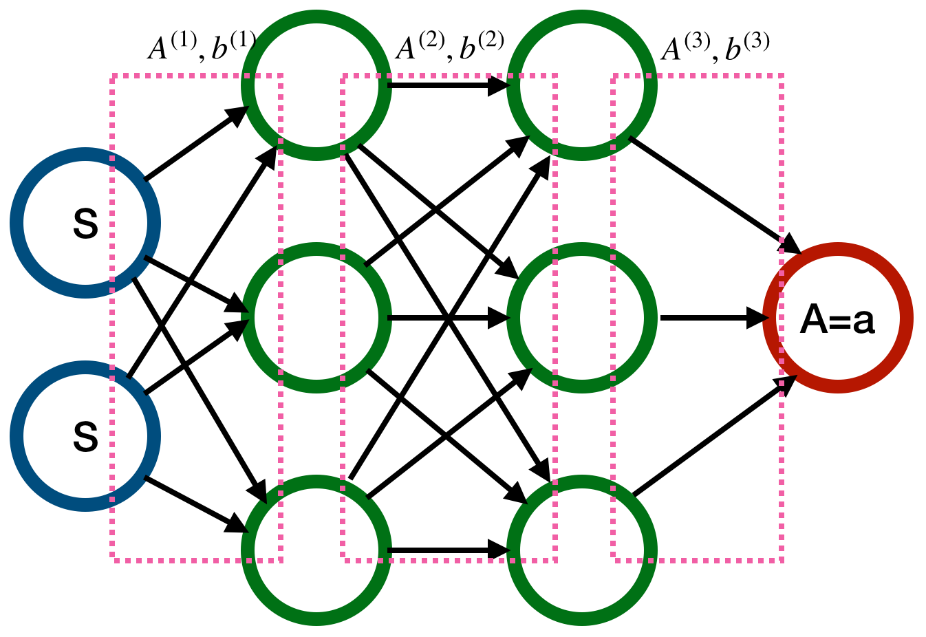
Figure 1: Illustration of a two-layer, fully connected DNN. The state is two-dimensional.

To solve (14), it is equivalent to solve

$$\operatorname*{arg\,min}_{\tau\in\mathcal{T}_{a}}\sum_{i=1}^{N}\sum_{t=0}^{T-1}\{\widetilde{\tau}_{i,t,a}-\tau(a,S_{i,t})\}^{2},$$ (15)

for each $a\neq a_{0}$. Many methods are available to solve (15), as it is essentially a nonparametric regression problem. In our implementation, we set $\mathcal{T}_{a}$ to the class of deep neural networks (DNNs), so as to capture the complex dependence between the reward and the state-action pair. The input of the network is a $d$-dimensional vector, corresponding to the state (coloured in blue in Figure 1). The hidden units (coloured in green) are grouped in a sequence of $L_{a}$ layers. Each unit in the hidden layer is determined as a nonlinear transformation of a linear combination of the nodes from the previous layer. We use $W_{a}$ to denote the total number of parameters. These parameters are updated by the Adam algorithm (Kingma and Ba, 2015).

5 Theoretical findings

We first summarize our theoretical findings. In Theorem 1, we provide a finite sample bias analysis of the pseudo outcome, proving its bias decays at a faster rate than the initial Q-estimator. In Theorem 2, we show our estimator for the optimal contrast achieves a faster rate of the convergence than the Q-estimator. In Theorem 3, we show the resulting optimal policy achieves a larger value than those computed by Q-learning type algorithms. Finally, we discuss a potential limitation of the proposed method. All the error bounds derived in this paper converge to zero when either $N$ or $T$ diverges to infinity. As commented in the introduction, this ensure our method is valid when applied to a wide range of real problems.

5.1 Finite sample bias analysis

In this section, we focus on deriving an error bound on the bias ${\mbox{E}}(\widetilde{Q}_{i,t,a}|S_{i,t})-Q^{\tiny{opt}}(S_{i,t},a)$ as a function of the total number of observations $NT$. We introduce the following conditions.

(A1) The state space $\mathbb{S}$ is compact. There exists some constant $\alpha>0$ such that

$$\begin{split}\lambda\left\{s\in\mathbb{S}:\max_{a}Q^{\tiny{opt}}(a,s)-\max_{a^{\prime}\in\mathbb{A}-\operatorname*{arg\,max}_{a}Q^{\tiny{opt}}(a,s)}Q^{\tiny{opt}}(a^{\prime},s)\leq\varepsilon\right\}=O(\varepsilon^{\alpha}),\end{split}$$ (16)

where $\lambda$ denotes the Lebesgue measure and the big-$O$ term in (16) is uniform in $0<\varepsilon<\delta$ for some sufficiently small $\delta>0$. By convention, $\max_{a^{\prime}\in\mathbb{A}-\operatorname*{arg\,max}_{a}Q^{\tiny{opt}}(a,s)}Q^{\tiny{opt}}(a^{\prime},s)=-\infty$ if the set $\mathbb{A}-\operatorname*{arg\,max}_{a}Q^{\tiny{opt}}(a,s)$ is empty.

(A2) $Q^{\tiny{opt}}(a,\cdot)$ is $p$-smooth and $\tau^{\tiny{opt}}(a,\cdot)$ is $p^{*}$-smooth for some $p^{*}<p$ and any $a$.

(A3) There exists some constant $0<c_{0}\leq 1$ such that the followings hold for any $a$ and $\ell$, with probability approaching 1,

$${\mbox{E}}_{(a,s)\sim p_{\infty}}|\widehat{Q}^{(\ell)}(a,s)-Q^{\tiny{opt}}(a,s)|^{2}=O\{(NT)^{-2p/(2p+d)}\},$$

$${\mbox{E}}_{(a,s)\sim p_{\infty},(a^{\prime},s^{\prime})\sim p_{\infty}}|\widehat{\omega}^{(\ell)}(a^{\prime},s^{\prime}|a,s)-\omega^{\widehat{\pi}^{(\ell)}}(a^{\prime},s^{\prime}|a,s)|^{2}=O\{(NT)^{-c_{0}}\}.$$

(A4) The process $\{(S_{t},A_{t},R_{t})\}_{t\geq 0}$ is stationary and exponentially $\beta$-mixing (see e.g., Bradley, 2005, for detailed definitions).

(A5) The probability density function $p_{\infty}$ is uniformly bounded away from zero.

In (A1), we require the state space to be continuous. When it is discrete, we can replace the Lebesgue measure with the counting measure. Our theories are equally applicable. we refer to the quantity $\max_{a}Q^{\tiny{opt}}(a,s)-\max_{a^{\prime}\in\mathcal{A}-\operatorname*{arg\,max}_{a}Q^{\tiny{opt}}(a,s)}Q^{\tiny{opt}}(a^{\prime},s)$ as the “margin” of the optimal Q-function. It measures the difference in value between $\pi^{\tiny{opt}}$ and the policy that assigns the best suboptimal treatment(s) at the first decision point and follows $\pi^{\tiny{opt}}$ subsequently. Such a margin-type condition is commonly used to bound the excess misclassification error (Tsybakov, 2004; Audibert and Tsybakov, 2007) and the regret of estimated optimal treatment regime (Qian and Murphy, 2011; Luedtke and van der Laan, 2016; Shi et al., 2020). Here, we impose Condition (A1) to bound the difference between $Q^{\widehat{\pi}^{(\ell)}}(S_{i,t},a)$ and $Q^{\tiny{opt}}(S_{i,t},a)$. This condition is mild. To elaborate, we consider a simple scenario where $\mathbb{A}=\{0,1\}$ and $a_{0}=0$. It follows that the margin equals $|\tau^{\tiny{opt}}(1,s)|$ if $\tau^{\tiny{opt}}(1,s)$ is nonzero and $+\infty$ otherwise. (16) is thus equivalent to the following,

$$\lambda\{s\in\mathbb{S}:0<|\tau^{\tiny{opt}}(1,s)|\leq\varepsilon\}=O(\varepsilon^{\alpha})$$ (17)

The above condition can be satisfied in a wide range of settings. We consider three examples to illustrate.

Example 6.

Suppose $\tau^{\tiny{opt}}(1,s)=0$ for any $s$. Then (17) is automatically satisfied. In this example, the two actions have the same effects. Any policy would achieve the same value.

Example 7.

Suppose $\inf_{s}|\tau^{\tiny{opt}}(1,s)|>0$. Then (17) is automatically satisfied for any sufficiently small $\varepsilon>0$. When the optimal contrast function is continuous, it requires $\tau^{\tiny{opt}}(1,s)$ to be always positive or negative as a function of $s$. As such, the optimal policy is nondynamic and will assign the same action at each time.

Example 8.

Consider the case where the state is one-dimensional. Suppose

$$\tau^{\tiny{opt}}(1,s)=\left\{\begin{array}[]{ll}s^{1/\alpha},&\textrm{if}~{}s>0;\\ 0,&\textrm{otherwise},\end{array}\right.$$

we have $\lambda\{s\in\mathbb{S}:0<|\tau^{\tiny{opt}}(1,s)|\leq\varepsilon\}=\lambda\{s\in\mathbb{S}:0<s\leq\varepsilon^{\alpha}\}=\varepsilon^{\alpha}$. (17) is thus satisfied.

In (A2), we assume the optimal contrast function is strictly “smoother” than the optimal Q-function. As we have discussed, this assumption holds under several cases. See Examples 1 and 2 in Section 3.2 for details.

In the first part of (A3), we assume the squared prediction loss of the estimated Q-function achieves a rate of $(NT)^{-2p/(2p+d)}$. As we have commented, this condition automatically holds when deep-Q network is used to fit the initial Q-estimator. The second part of (A3) is mild as the constant $c_{0}$ could be arbitrarily small. Suppose some parametric model (e.g., linear) is imposed to learn $\widehat{\omega}^{(\ell)}$. When the model is correctly specified, then we have $c_{0}=1$. When kernels are used for function approximation, the rate $c_{0}$ can be established in a similar manner as in Theorem 5.4 of Liao et al. (2020).

(A4) requires the $\beta$-mixing coefficients of the process $\{(S_{t},A_{t},R_{t})\}_{t\geq 0}$ to decay to zero at an exponential rate. These coefficients characterize the temporal dependence of the observations and are equal to zero when the data are independent. The smaller the coefficients, the weaker the dependence. When the propensity score is stationary over time, $\{(S_{t},A_{t},R_{t})\}_{t\geq 0}$ forms a time-homogeneous Markov chain. (A4) is automatically satisfied when the Markov chain is geometrically ergodic (see Theorem 3.7 of Bradley, 2005). Geometric ergodicity is less restrictive than those imposed in the existing reinforcement learning literature that requires observations to be independent (see e.g., Degris et al., 2012) or to follow a uniform-ergodic Markov chain (see e.g., Zou et al., 2019). We also remark that the stationarity assumption in (A1) is assumed only to simplify the technical proof. Our theoretical results are equally applicable even without this condition (see e.g., the proof of Lemma 3 of Shi et al., 2020).

(A5) is very similar to the positivity assumption imposed in single-stage decision making. These assumptions enable us to derive the following theorem.

Theorem 1.

Assume (A1)-(A5) hold. $\widehat{Q}^{(\ell)}$, $\widehat{\omega}^{(\ell)}$ and the rewards are uniformly bounded. Then there exists some constant $\bar{c}>p/(2p+d)$ such that for any $a\in\mathbb{A}$,

$$\frac{1}{NT}\sum_{i,t}{\mbox{E}}|{\mbox{E}}(\widetilde{Q}_{i,t,a}|S_{i,t})-Q^{\tiny{opt}}(S_{i,t},a)|=O\{(NT)^{-\bar{c}}\}.$$

Theorem 1 states that the conditional bias of $\widetilde{Q}_{i,t,a}$ decays at a rate of $(NT)^{-\bar{c}}$ on average. In comparison, under (A3), the squared prediction loss of the initial Q-estimator decays at a rate of $(NT)^{-2p/(2p+d)}$. Suppose the square bias and variance of $\widehat{Q}^{(\ell)}$ are of the same order. Then we expect ${\mbox{E}}\{\widehat{Q}^{(\ell)}(a,S_{i,t})|S_{i,t}\}$ to approach $Q^{\tiny{opt}}(S_{i,t},a)$ at a rate of $(NT)^{-p/(2p+d)}$. Since $\bar{c}>p/(2p+d)$, biases of our pseudo outcomes are much smaller than the initial Q-estimators.

5.2 Efficiency enhancement

In this section, we establish the convergence rates of the estimated contrast function and the derived optimal policy. Without loss of generality, we assume the state space $\mathbb{S}=[0,1]^{d}$. We write $a_{n}\asymp b_{n}$ for two sequences $\{a_{n}\}_{n}$ and $\{b_{n}\}_{n}$ if there exists some universal constant $c\geq 1$ such that $c^{-1}a_{n}\leq b_{n}\leq ca_{n}$ for all $n$.

Theorem 2.

Assume the conditions in Theorem 1 hold. Then there exists DNN class $\{\mathcal{T}_{a}\}_{a}$ with $L_{a}\asymp\log(NT)$ and $W_{a}\asymp(NT)^{C}\log(NT)$ for some $C>d/(2p+d)$ and any $a\neq a_{0}$ such that with probability approaching $1$,

$${\mbox{E}}_{s\sim p_{\infty}}|\widehat{\tau}(a,s)-\tau^{\tiny{opt}}(a,s)|^{2}=O\{(NT)^{-c_{1}}\},$$

for some constant $2p/(2p+d)<c_{1}\leq 2p^{*}/(2p^{*}+d)$, where the expectation is taken with respect to the stationary state distribution.

Theorem 2 formally shows that our estimated contrast function converges at a faster rate than the Q-function computed by Q-learning type-estimators, leading to the desired efficiency enhancement property. To illustrate why the estimated contrast converges faster, suppose we have access to some unbiased pseudo outcome for $\tau(a,S_{i,t})$. Then under (A2), the estimated contrast function would converge at a minimax optimal rate of $(NT)^{-p^{*}/(2p^{*}+d)}$, which is much faster than that of the Q-estimator. In practice, we do not have access to unbiased pseudo outcomes. As such, the rate would depend on the bias of the pseudo outcome $\widetilde{Q}_{i,t,a}-\widetilde{Q}_{i,t,a_{0}}$. Nonetheless, the efficiency enhancement property holds as long as the bias decays faster than the convergence rate of the Q-estimator. The latter assertion is confirmed in Theorem 1.

We next show this in turn leads to an improvement in the value. More specifically, for any policy $\pi$, define the integrated value function $\mathcal{V}(\pi)=\int_{\mathbb{S}}V^{\pi}(s)\nu_{0}(s)ds$ where $\nu_{0}$ denotes the density function of $S_{0}$. Let $\widehat{\pi}^{\tau}$ denote the derived policies based on the estimated contrast function $\widehat{\tau}$.

Theorem 3.

Assume the conditions in Theorem 1 hold and $\nu_{0}$ is uniformly bounded from above. Then

$$\mathcal{V}({\pi^{\tiny{opt}}})-{\mbox{E}}\mathcal{V}(\widehat{\pi}^{\tau})=O\{(NT)^{-\alpha_{0}c_{1}/2}\},$$

where $\alpha_{0}=(2+2\alpha)/(\alpha+2)>1$ and $\alpha$ is defined in (A1).

Let $\widehat{Q}$ denotes a Q-learning type estimator that satisfies

$${\mbox{E}}_{(a,s)\sim p_{\infty}}|\widehat{Q}(a,s)-Q^{\tiny{opt}}(a,s)|^{2}=O\{(NT)^{-2p/(2p+d)}\},$$ (19)

and $\widehat{\pi}^{Q}$ be the derived policy based on $\widehat{Q}$. Similar to Theorem 3, we can show that ${\mbox{E}}\mathcal{V}(\widehat{\pi}^{Q})$ converges at a rate of $\alpha_{0}p/(2p+d)$. Based on the fact that $c_{1}>2p/(2p+d)$, it is clear that the value of our estimated policy converges to the optimal value at a faster rate than those of policies computed by Q-learning type algorithms.

The convergence rates in Theorems 2 and 3 relies crucially on the exponent $\alpha$ in the margin condition (A1) and the convergence rate of the estimated density ratio in (A3), i.e., $(NT)^{-c_{0}}$. The following corollary shows that under certain conditions on $\alpha$ and $c_{0}$, the exponent $c_{1}$ in both theorems achieve a maximum value of $2p^{*}/(2p^{*}+d)$.

Corollary 1.

Suppose the conditions in Theorems 2 and 3 hold. Suppose $c_{0}\geq 2p^{*}/(2p^{*}+d)-2p/(2p+d)$ and $\alpha\geq 2[2-\{p^{*}/(2p^{*}+d)\}/\{p/(2p+d)\}]^{-1}-2$. Then with proper choice of the DNN class $\{\mathcal{T}_{a}\}_{a}$, we have for any $a\neq a_{0}$ that

$${\mbox{E}}_{s\sim p_{\infty}}|\widehat{\tau}(a,s)-\tau^{\tiny{opt}}(a,s)|^{2}=O\{(NT)^{-2p^{*}/(2p^{*}+d)}\},$$

with probability approaching $1$, and that $\mathcal{V}({\pi^{\tiny{opt}}})-{\mbox{E}}\mathcal{V}(\widehat{\pi}^{\tau})=O\{(NT)^{-\alpha_{0}p^{*}/(2p^{*}+d)}\}$.

Notice that we do not require the optimal policy to be unique in order to establish the regret bound of the estimated optimal policy. This is because our proposal is value-based which derives the optimal policy using the estimated advantage function. The advantage function is well-defined despite that the optimal policy might not be unique, and the regret bound decays to zero as long as the estimated advantage function is consistent. To elaborate, let us revisit Example 8. By definition, when the state is nonpositive, both actions are optimal. The uniqueness assumption is thus violated. Nonetheless, the regret is zero since choosing either action is optimal.

Finally, we remark that although the proposed contrast function estimator converges at a faster rate than Q-learning type estimators, these rates are asymptotic. A potential limitation of the proposed method is that our estimated contrast function might have larger variance than Q-learning type estimators in finite samples, due to the use of importance sampling in constructing the pseudo outcomes. This reflects a bias-variance trade-off. The proposed A-learning method might suffer from a larger variance whereas Q-learning type methods might suffer from a larger bias. This observation is consistent with the findings in the literature on learning DTRs (see e.g., Schulte et al., 2014).

6 Simulations

We evaluate the performance of our method using two synthetic datasets generated by the Open AI Gym environment (see https://gym.openai.com/) in this section. We consider the following Q-learning type baseline methods: (a) DQN; (b) double DQN (DDQN); (c) quantile DQN (QR-DQN). See Examples 3-5 for detailed discussion of these algorithms. As we have commented in Section 4, our policy optimization procedure at Step 2 is generally applicable to any Q-learning type algorithms. To validate this claim, for each of these Q-learning type methods in (a)-(c), we couple it with sample splitting to compute the initial Q-estimator in Step 2 based on each half of the data, and apply our proposal in Steps 3-5 to learn an optimal policy. This yields three estimated optimal policies. We denote them by (d) SEAL-DQN, (e) SEAL-DDQN and (f) SEAL-QR-DQN, respectively. Then we contrast them with the corresponding Q-learning type algorithms in (a)-(c) fitted based on the entire offline data. In addition to these baseline methods, we also consider three recently developed offline policy optimization methods in the computer science literature, including (g) batch-constrained deep Q-learning (BCQ, Fujimoto et al., 2019), (h) random ensemble mixture (REM, Agarwal et al., 2020) and (i) bootstrapping error accumulation reduction (BEAR, Kumar et al., 2019). We compare them with the proposed procedure based on QR-DQN, which yields the best performance among (d)-(f).

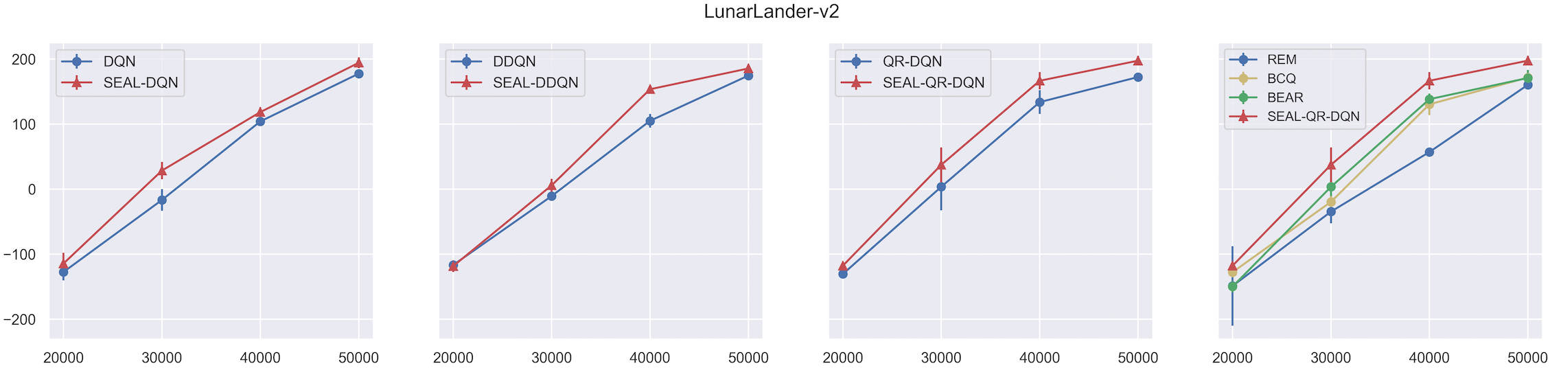
Figure 2: Synthetic data analysis results for LunarLander-v2. Horizontal axis represents the number of training steps used to train the initial Q-estimator based on half the data as well as the baseline method based on the entire dataset. Vertical axis represents the average reward of 100 evaluations. The error bar corresponds to the 95% confidence interval for the value, constructed based on 10 replications. The first three panels compare one baseline Q-learning algorithm (DQN, DDQN, QR-DQN) with our method that uses such a baseline to compute the initial Q-estimator. The last panel compares the proposed algorithm based on QR-DQN against REM, BCQ and BEAR.

6.1 LunarLander-v2

We conduct experiments in an OpenAI Gym environment, LunarLander-v2. Detailed description about this environment can be found at LunarLander-v2. To generate the data, we train a QR-DQN agent $500$K time steps, with learning rate $0.0005$. The estimated policy after $500$K time steps is near optimal and solves the environment (e.g., achieves a score of 200 on average). The state-of-the-art optimal average reward is over 250. We then terminate the training process, store all the generated trajectories encountered during the online training process and use them as the offline data. The behavior policy corresponds to the $\epsilon$-greedy policy used to train the online QR-DQN agent with $\epsilon=0.1$. The offline dataset consists of 1089 trajectories. Each trajectory lasts for 459 time steps on average. The average immediate reward equals 118.

The training data consist of 200 trajectories randomly sampled out of the 1089 trajectories. For each of the estimated optimal policy learned based on (a)-(i), we evaluate its value by computing the mean reward of 100 trajectories generated in the environment under this policy. We repeat the entire data generating process, the training and evaluation procedures 10 times with different random seeds. We also vary the number of training steps for the initial Q-estimator and apply the proposed method to each of the estimated Q-functions. For fair comparison, we use the same number of training steps (i.e., 20K, 30K, 40K or 50K) to train the baseline policy.

Reported in Figure 2 are the values of the estimated policies computed by (a)-(i) as well as the associated 95% confidence intervals, with different number of training steps. We summarize our findings as follows: (1) The proposed procedure achieves a larger value compared to the baseline methods in most cases; (2) Our improvement is significant in many cases, as suggested by the error bar; (3) All the methods get improved as the number of training steps increases.

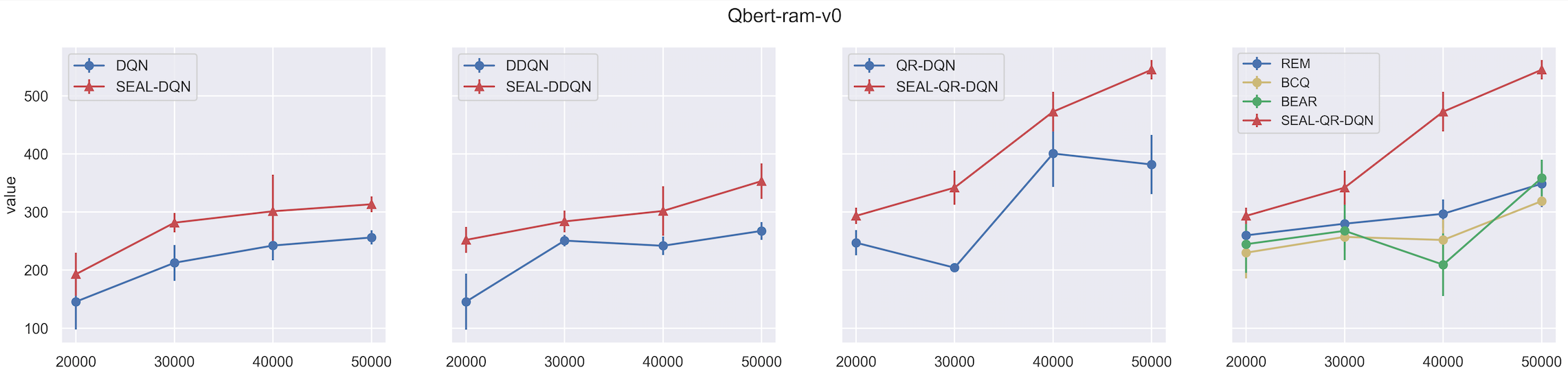
Figure 3: Synthetic data analysis results for Qbert-ram-v0. Same legend as Figure 2.

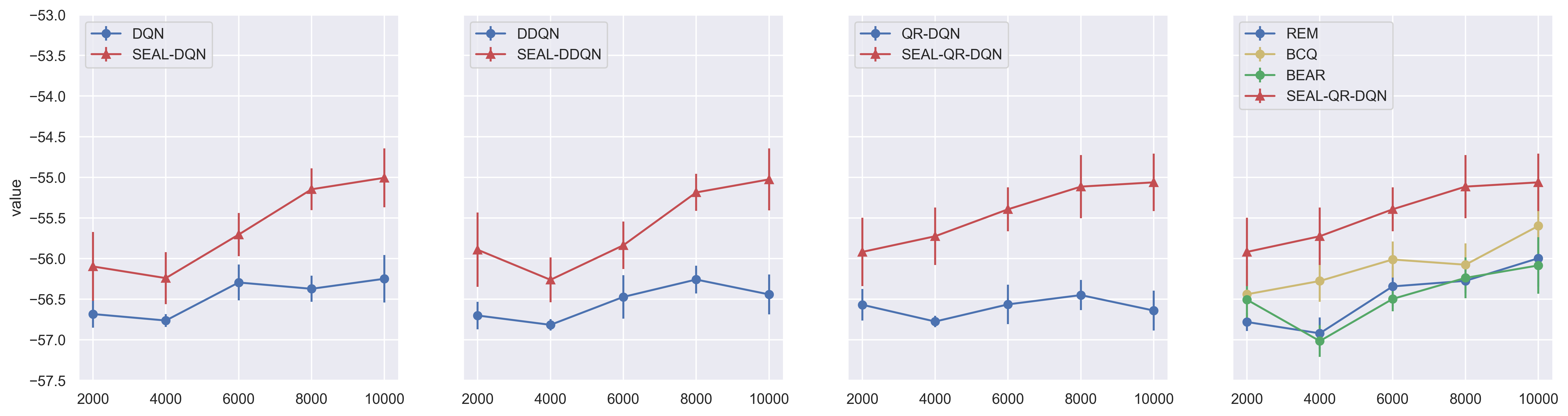
Figure 4: Real data analysis results. Horizontal axis represents the number of training steps. Same legend as Figure 2.

6.2 Qbert-ram-v0

We next conduct experiments in another environment, Qbert-ram-v0. The best 100-episode average reward for Qbert-ram-v0 is $586.00\pm 12.16$. We similarly train a Quantile DQN agent to generate 1373 trajectories. Each trajectory lasts for 364 time steps on average. The average return per trajectory equals 278. We similarly compare our procedures (d)-(f) with the baseline methods (a)-(c) and (g)-(i). Results are depicted in Figure 3. Overall, findings are very similar to those in Section 6.1. We notice that the performances of some deep Q-learning methods drop when the number of training step increases and cannot even improve after a few more iterations. We discuss this in detail in Section 8.4 to save space.

Finally, it can very computationally expensive to implement deep RL algorithms in LunarLander-v2 and Qbert-ram-v0. For instance, in our implementation, it took a few hours to run one simulation. As such, our simulation results are aggregated over 10 runs only. We also remark that beginning with DQN, 5 or less runs are common in the existing RL literature, as it is often computationally prohibitive to evaluate more runs (Agarwal et al., 2021); see also the numerical studies in Mnih et al. (2015); Silver et al. (2016); Kumar et al. (2019); Agarwal et al. (2020).

7 The OhioT1DM dataset

In this section, we use the OhioT1DM Ddataset (Marling and Bunescu, 2018) to illustrate the usefulness of our new method in moblie health applications. The data contains continuous measurements for six patients with type 1 diabetes over eight weeks. The objective is to learn an optimal policy that maps patients’ time-varying covariates into the amount of insulin injected at each time to maximize patients’ health status.

In our experiment, we divide each day of follow-up into one hour intervals and a treatment decision is made every hour. We consider three important time-varying state variables, including the average blood glucose level $G_{t}$ during the one hour interval $(t-1,t]$, the carbohydrate estimate for the meal $C_{t}$ during $(t-1,t]$ and $\text{Ex}_{t}$ which measures exercise intensity during $(t-1,t]$. At time $t$, we define the action $A_{t}$ by discretizing the amount of insulin $\text{In}_{t}$ injected. The reward $R_{t}$ is chosen according to the Index of Glycemic Control (Rodbard, 2009) that is a deterministic function $G_{t+1}$. Detailed definitions of $A_{t}$ and $R_{t}$ are given in Appendix B. We will receive a low reward if the patient’s average blood glucoses level is outside the range $[80,140]$. Let $X_{t}=(G_{t},C_{t},\hbox{Ex}_{t})$. We define the state $S_{t}$ by concatenating measurements over the last four decision points, i.e., $S_{t}=(X_{t-3}^{T},A_{t-3},\cdots,X_{t})^{\top}$. This ensures the Markov assumption is satisfied (Shi et al., 2020). The number of decision points for each patient in the OhioT1DM dataset ranges from 1119 to 1288. Transitions across different days are treated as independent trajectories. This yields 279 trajectories in total.

We use cross-validation to evaluate the performance of different algorithms. Specifically, we apply each of the method in (a)-(i) to the training dataset to learn an optimal policy. Then we apply the fitted Q-evaluation (FQE, Le et al., 2019) algorithm to the testing dataset to evaluate the values of these policies. FQE is very similar to FQI. It iteratively update the state-action value using supervised learning algorithms. See Algorithm 1 in Appendix B for details. In our implementation, we set the function approximator $\mathcal{F}$ to a class of DNN and apply deep learning to update the value. These estimated values are further aggregated over different training/testing combinations. Finally, we repeat this procedure 10 times with different random seeds to further aggregated the values. Results are reported in Figure 4. It can be seen that the proposed method performs significant better than other baseline methods in most cases.

8 Discussion

This section is organized as follows. In Sections 8.1 and 8.2, we discuss extensions of our proposal to the continuous action space. In Section 8.3, we discuss the $p$-smoothness assumption. Finally, in Section 8.4, we discuss some offline RL algorithms and the pessimistic principle.

8.1 Action discretization

One possible approach to handle continuous action space is to first discretize the action space and then apply the proposed method for policy learning. Suppose the action space is one-dimensional, as in personalized dose finding and dynamic pricing. Then we can extend the jump interval-learning method (Cai et al., 2021) to sequential decision making for adaptively discretizing the action space. The baseline action can be similarly determined after we obtain the discretization.

Specifically, the jump interval learning method was originally designed in contextual bandit settings for deriving interval-valued policies. The main idea is to partition the action space into a set of disjoint intervals such that within each interval, the Q-function is a constant function of the action. In this section, we outline an extension of this method to sequential decision making. Without loss of generally, assume the action space $\mathbb{A}=[0,1]$. To illustrate the method, we assume the transition function is a piecewise function of the action, i.e., there exist a set of disjoint intervals $\mathbb{D}$ that cover $\mathbb{A}$ and satisfy that

$$q(s^{\prime};a,s)=\sum_{\mathcal{I}\in\mathbb{D}}\mathbb{I}(a\in\mathcal{I})q_{\mathcal{I}}(s^{\prime};s),$$

for any $s,s^{\prime}$ and a set of transition functions $q_{\mathcal{I}}$. Under such an assumption, any Q-function is a piecewise function of the action. To identify $\mathbb{D}$, we can couple fitted Q-iteration with jump-interval learning and iteratively solve the following optimization problem based on dynamic programming (Friedrich et al., 2008),

$$(\widehat{\mathbb{D}},\{\widehat{Q}_{\mathcal{I}}^{(k)}:\mathcal{I}\in\mathbb{D}\})=\operatorname*{arg\,min}\sum_{\mathcal{I}}\sum_{i,t}\mathbb{I}(A_{i,t}\in\mathcal{I})[R_{i,t}+\gamma\max_{\mathcal{I}}\widehat{Q}_{\mathcal{I}}^{(k-1)}(S_{i,t+1})-\widehat{Q}_{\mathcal{I}}^{(k)}(S_{i,t})]^{2}+\gamma|\widehat{\mathbb{D}}|,$$

for $k=1,\cdots,K$ and some tuning parameter $\gamma>0$, where $|\widehat{\mathbb{D}}|$ denotes the number of intervals in $\widehat{\mathbb{D}}$. The final output $\widehat{\mathbb{D}}$ yields a set of action intervals, based on which we can define a categorical action variable $A_{i,t}^{*}$ whose value depends on the interval that the original action $A_{i,t}$ belongs to. Finally, we apply the proposed method to the transformed dataset $\{(S_{i,t},A_{i,t}^{*},R_{i,t})\}_{i,t}$ for policy learning.

8.2 Kernel-based method

Another potential approach is to adopt kernel-based methods that leverage treatment proximity to allow continuous actions. In that case, we can apply kernel density estimation to learn the marginal probability density function of the action and set the baseline action to the one that maximizes the estimated density function.

Specifically, kernel-based methods are commonly used for policy learning and evaluation with continuous action space (see e.g., Chen et al., 2016; Kallus and Zhou, 2018; Colangelo and Lee, 2020). Notice that the proposed method requires to weight each observation by the importance sampling ratio $\mathbb{I}(A_{i,t}=a)/{\mbox{Pr}}(A_{i,t}=a|S_{i,t})$ to construct the pseudo outcome. When the actions are continuous, the indicator function $\mathbb{I}(A_{i,t}=a)$ equals zero almost surely for any $i$ and $t$. Consequently, naively applying the importance sampling ratio would yield a biased estimator. To address this concern, we can employ kernel-based methods to replace the indicator function $\mathbb{I}(A_{i,t}=a)$ with a kernel function $K\{(A-a)/h\}$ for some bandwidth parameter $h$, and probability mass function ${\mbox{Pr}}(A_{i,t}=a|S_{i,t})$ with the corresponding probability density function. The baseline action can be set to the argmax of $\sum_{i,t}K\{(A_{i,t}-a)/h\}$.

8.3 The $p$-smoothness assumption

We discuss the $p$-smoothness assumption in this section. First, as commented in the main text, the $p$-smoothness assumption is likely to hold in mobile health studies. In these applications, the state corresponds to some time-varying variables that measure the health status of a given subject. It is expected that the system dynamics would vary smoothly as a function of these variables. In the literature, a number of papers also use a smooth transition function to simulate the environment in healthcare applications (Ertefaie, 2014; Luckett et al., 2020; Shi et al., 2020; Li et al., 2022). In addition, the reward is usually a deterministic function of the current state-action pair and future state; see e.g., the definition of the reward in our application in Appendix B. As such, as long as the transition function is $p$-smooth, so is the reward function as well.

Second, the $p$-smoothness assumption is not likely to hold in many OpenAI gym environments where the state variables are all discrete or the state transition is deterministic. Nonetheless, we remark that it can be seen from our simulation results that the proposed method works better than or comparable to existing Q-learning algorithms.

8.4 Offline RL and the pessimistic principle

As pointed out by one of the referee, it can be seen from Figure 3 that the performances of some deep Q-learning methods drop when the number of training step increases and cannot even improve after a few more iterations. We suspect this is due to that some state-action pairs are less explored in the offline dataset, leading to the violation of the positivity assumption (A5). In that case, increasing the number of training steps might overfit the data and worsen the performance of the resulting policy. Similar phenomena have been observed in the existing RL literature (see e.g., Kumar et al., 2019).

Many offline RL algorithms such as BCQ, REM and BEAR adopted the pessimistic principle (see e.g., Levine et al., 2020; Jin et al., 2021; Xie et al., 2021) and proposed to learn a “conservative” Q-function by penalizing the values evaluated at those “out-of-distribution” state-action pairs. These algorithms are shown to outperform the standard Q-learning algorithm in offline domains when (A5) is violated to some extent. We suspect that reducing the number of training steps is equivalent to penalize the Q-function to some extent to avoid overfitting. As such, increasing the number of training steps would make things worse. It is interesting to investigate how to couple the pessimistic principle with our proposal to further improve the estimated policy. However, this is beyond the scope of the current paper. We leave it for future research.

Appendix A Proofs

We prove Theorems 1 and 2 in this section. Theorem 3 can be proven in a similar manner as Theorem 4 of Shi et al. (2020). We omit its proof for brevity. Throughout this section, we use $c$ and $C$ to denote some generic constants whose values are allowed to vary from place to place. For any two positive sequences $\{a_{t}\}_{t\geq 1}$ and $\{b_{t}\}_{t\geq 1}$, we write $a_{t}\preceq b_{t}$ if there exists some constant $c>0$ such that $a_{t}\leq cb_{t}$ for any $t$. The notation $a_{t}\preceq 1$ means $a_{t}=O(1)$.

A.1 Proof of Theorem 1

Let $\{\beta(q)\}_{q\geq 0}$ denote the $\beta$-mixing coefficients (see e.g., Bradley, 2005, for detailed definitions) of the process $\{(S_{t},A_{t},R_{t})\}_{t\geq 0}$. Under the given conditions, we obtain $\beta(q)\to 0$ as $q\to\infty$. Let $b(a|S_{t})$ denote the propensity score ${\mbox{Pr}}(A_{t}=a|S_{t})$ for any $a\in\mathbb{A}$. Let $\widehat{V}^{(\ell)}(s)$ denote the estimated optimal value function $\sum_{a\in\mathbb{A}}\pi^{\widehat{\ell}}(a|s)\widehat{Q}^{(\ell)}(a,s)$ for any $s\in\mathbb{S}$. By definition,

$$\widetilde{Q}_{i,t,a}=\widehat{Q}^{(\ell)}(a,S_{i,t})+\frac{\mathbb{I}(A_{i,t}=a)}{b(a|S_{i,t})}\{R_{i,t}+\gamma\widehat{V}^{(\ell)}(S_{i,t+1})-\widehat{Q}^{(\ell)}(A_{i,t},S_{i,t})\}+\frac{\gamma}{1-\gamma}\widetilde{\eta}_{i,t,a}.$$

Note that

$${\mbox{E}}[\widetilde{\eta}_{i,t,a}|S_{i,t},\{O_{j,t}\}_{1\leq j\leq N,0\leq t<T}]={\mbox{E}}[\eta_{i,t,a}|S_{i,t},\{O_{j,t}\}_{1\leq j\leq N,0\leq t<T}].$$

As such, the conditional mean of $\widetilde{Q}_{i,t,a}$ is the same as $Q_{i,t,a}$, defined as

$$Q_{i,t,a}=\widehat{Q}^{(\ell)}(a,S_{i,t})+\frac{\mathbb{I}(A_{i,t}=a)}{b(a|S_{i,t})}\{R_{i,t}+\gamma\widehat{V}^{(\ell)}(S_{i,t+1})-\widehat{Q}^{(\ell)}(A_{i,t},S_{i,t})\}+\frac{\gamma}{1-\gamma}\eta_{i,t,a}.$$

In the following, we break the proof into three steps. In the first step, we show

$$\begin{split}{\mbox{E}}\left[\left.\widehat{Q}^{(\ell)}(a,S_{i,t})+\frac{\mathbb{I}(A_{i,t}=a)}{b(a|S_{i,t})}\{R_{i,t}+\gamma\widehat{V}^{(\ell)}(S_{i,t+1})-\widehat{Q}^{(\ell)}(A_{i,t},S_{i,t})\}\right|S_{i,t},\{O_{j,t}\}_{j\in\mathcal{I}_{\ell}^{c},0\leq t<T}\right]\\ =r(a,S_{i,t})+{\mbox{E}}\{\widehat{V}^{(\ell)}(S_{i,t+1})|S_{i,t},A_{i,t}=a\}=r(a,S_{i,t})+\gamma\int_{s^{\prime}}\widehat{V}^{(\ell)}(s^{\prime})q(s^{\prime};S_{i,t},a)ds^{\prime}.\end{split}$$ (20)

Note that $\eta_{i,t,a}$ can be decompose into

$$\eta_{i,t,a}=\frac{(|\mathcal{I}_{\ell}|-1)T}{|\mathcal{I}_{\ell}|T-1}\eta_{i,t,a,1}+\frac{T-1}{|\mathcal{I}_{\ell}|T-1}\eta_{i,t,a,2},$$ (21)

where $\eta_{i,t,a,1}$ and $\eta_{i,t,a,2}$ are defined by

$$\frac{1}{(|\mathcal{I}_{\ell}|-1)T}\sum_{\begin{subarray}{c}i^{\prime}\in\mathcal{I}_{\ell},i^{\prime}\neq i\\ 0\leq t^{\prime}<T\end{subarray}}\widehat{\omega}^{(\ell)}(A_{i^{\prime},t^{\prime}},S_{i^{\prime},t^{\prime}}|a,S_{i,t})\{R_{i^{\prime},t^{\prime}}+\gamma\widehat{V}^{(\ell)}(S_{i^{\prime},t^{\prime}+1})-\widehat{Q}^{(\ell)}(S_{i^{\prime},t^{\prime}},A_{i^{\prime},t^{\prime}})\},$$

$$\frac{1}{T-1}\sum_{\begin{subarray}{c}0\leq t^{\prime}<T\\ t^{\prime}\neq t\end{subarray}}\widehat{\omega}^{(\ell)}(S_{i,t^{\prime}};S_{i,t},a)\{R_{i^{\prime},t^{\prime}}+\gamma\widehat{V}^{(\ell)}(S_{i,t^{\prime}+1})-\widehat{Q}^{(\ell)}(S_{i,t^{\prime}},A_{i,t^{\prime}})\},$$

respectively.

In the second step, we show that

$$\begin{split}\quad\frac{1}{NT}\sum_{\begin{subarray}{c}\ell\in\{1,\cdots,\mathbb{L}\}\\ i\in\mathcal{I}_{\ell}\end{subarray}}\sum_{0\leq t<T}{\mbox{E}}\left|{\mbox{E}}\left[\eta_{i,t,a,1}-(1-\gamma)\int_{s^{\prime}}\{V^{\widehat{\pi}^{(\ell)}}(s^{\prime})-\widehat{V}^{(\ell)}(s^{\prime})\}q(s^{\prime};S_{i,t},a)ds^{\prime}|S_{i,t}\right]\right|\\ \leq O(1)(NT)^{-\kappa_{1}},\end{split}$$ (22)

where $\kappa_{1}=p/(2p+d)+c_{0}/2$ and satisfies $p/(2p+d)<\kappa_{1}<1/2$ under the given conditions on $c_{0}$, and $O(1)$ denotes some positive constant that is independent of $i,t,a,\ell$. Specifically, we will decompose $\eta_{i,t,a,1}$ into three terms and investigate the conditional mean of each of these terms in detail.

In the last step, we apply Berbee’s coupling lemma (see Lemma 4.1 in Dedecker and Louhichi, 2002) to show that

$$\begin{split}{\mbox{E}}\left|{\mbox{E}}\left[\eta_{i,t,a,2}-(1-\gamma)\int_{s^{\prime}}\{V^{\widehat{\pi}^{(\ell)}}(s^{\prime})-\widehat{V}^{(\ell)}(s^{\prime})\}q(s^{\prime};S_{i,t},a)ds^{\prime}|S_{i,t}\right]\right|\\ \leq O(1)T^{-1}\log T.\end{split}$$ (23)

Combining (20), (22) and (23) yields that

$$\frac{1}{NT}\sum_{\begin{subarray}{c}\ell\in\{1,\cdots,\mathbb{L}\}\\ i\in\mathcal{I}_{\ell}\end{subarray}}\sum_{0\leq t<T}{\mbox{E}}\left|{\mbox{E}}\left[\widetilde{Q}_{i,t,a}|S_{i,t})-r(a,S_{i,t})-\gamma\int_{s^{\prime}}V^{\widehat{\pi}^{(\ell)}}(s^{\prime})q(s^{\prime};S_{i,t},a)ds^{\prime}|S_{i,t}\right]\right|$$

$$\leq O(1)(NT)^{-\kappa_{1}}.$$

To complete the proof, it remains to show

$$\max_{i,t}\left|{\mbox{E}}\left[\int_{s^{\prime}}\{V^{\widehat{\pi}^{(\ell)}}(s^{\prime})-V^{\tiny{opt}}(s^{\prime})\}q(s^{\prime};S_{i,t},a)ds^{\prime}|S_{i,t}\right]\right|\leq O(1)(NT)^{-\kappa_{2}},$$ (24)

for some $\kappa_{2}>p/(2p+d)$ with probability tending to $1$. Using similar arguments in the proof of Theorem 4 of Shi et al. (2020), one can show (24) holds with $\kappa_{2}=p(2+2\alpha)/\{(d+2p)(2+\alpha)\}>p/(2p+d)$ under the margin-type condition in (A1). The proof is thus completed. Next, we give detailed proofs for each step.

A.1.1 Step 1

With some calculations, we have

$${\mbox{E}}\left[\left.\widehat{Q}^{(\ell)}(a,S_{i,t})+\frac{\mathbb{I}(A_{i,t}=a)}{b(a|S_{i,t})}\{R_{i,t}-\widehat{Q}^{(\ell)}(A_{i,t},S_{i,t})\}\right|S_{i,t},\{O_{j,t}\}_{j\in\mathcal{I}_{\ell}^{c},0\leq t\leq T}\right]$$

$$=\widehat{Q}^{(\ell)}(a,S_{i,t})-\widehat{Q}^{(\ell)}(a,S_{i,t})+r(a,S_{i,t})=r(a,S_{i,t}),$$

and

$${\mbox{E}}\left[\left.\frac{\mathbb{I}(A_{i,t}=a)}{b(a|S_{i,t})}\widehat{V}^{(\ell)}(S_{i,t+1})\right|S_{i,t},\{O_{j,t}\}_{j\in\mathcal{I}_{\ell}^{c},0\leq t<T}\right]={\mbox{E}}\{\widehat{V}^{(\ell)}(S_{i,t+1})|S_{i,t},A_{i,t}=a\}.$$

This yields (20). The proof of Step 1 is thus completed.

A.1.2 Step 2

We decompose $\eta_{i,t,a,1}$ into $\eta_{i,t,a,3}+\eta_{i,t,a,4}+\eta_{i,t,a,5}$ where

$$\eta_{i,t,a,3} = \frac{1}{(|\mathcal{I}_{\ell}|-1)T}\sum_{\begin{subarray}{c}i^{\prime}\in\mathcal{I}_{\ell},i^{\prime}\neq i\\ 0\leq t^{\prime}<T\end{subarray}}\omega^{\widehat{\pi}^{(\ell)}}(A_{i^{\prime},t^{\prime}},S_{i^{\prime},t^{\prime}}|a,S_{i,t})\widehat{\varepsilon}^{(\ell)}_{i^{\prime},t^{\prime}},$$

$$\eta_{i,t,a,4} = \frac{1}{(|\mathcal{I}_{\ell}|-1)T}\sum_{\begin{subarray}{c}i^{\prime}\in\mathcal{I}_{\ell},i^{\prime}\neq i\\ 0\leq t^{\prime}<T\end{subarray}}\{\widehat{\omega}^{(\ell)}(A_{i^{\prime},t^{\prime}},S_{i^{\prime},t^{\prime}}|a,S_{i,t})-\omega^{\widehat{\pi}^{(\ell)}}(A_{i^{\prime},t^{\prime}},S_{i^{\prime},t^{\prime}}|a,S_{i,t})\}\varepsilon_{i^{\prime},t^{\prime}},$$

$$\eta_{i,t,a,5} = \frac{1}{(|\mathcal{I}_{\ell}|-1)T}\sum_{\begin{subarray}{c}i^{\prime}\in\mathcal{I}_{\ell},i^{\prime}\neq i\\ 0\leq t^{\prime}<T\end{subarray}}\{\widehat{\omega}^{(\ell)}(A_{i^{\prime},t^{\prime}},S_{i^{\prime},t^{\prime}}|a,S_{i,t})-\omega^{\widehat{\pi}^{(\ell)}}(A_{i^{\prime},t^{\prime}},S_{i^{\prime},t^{\prime}}|a,S_{i,t})\}(\widehat{\varepsilon}^{(\ell)}_{i^{\prime},t^{\prime}}-\varepsilon_{i^{\prime},t^{\prime}}),$$

where $\varepsilon_{i,t}$ denotes the Bellman residual $R_{i,t}+\gamma V^{\widehat{\pi}^{(\ell)}}(S_{i,t+1})-Q^{\widehat{\pi}^{(\ell)}}(A_{i,t},S_{i,t})$ and $\widehat{\varepsilon}_{i,t}^{(\ell)}$ denotes its estimator by plugging in $\widehat{Q}^{(\ell)}$ and $\widehat{V}^{(\ell)}$ for $Q^{\widehat{\pi}^{(\ell)}}$ and $V^{\widehat{\pi}^{(\ell)}}$, respectively.

Notice that for any $i^{\prime}\in\mathcal{I}_{\ell}$, $i^{\prime}\neq i$, $0\leq t^{\prime}<T$, $O_{i^{\prime},t^{\prime}}$ is independent of $O_{i,t}$. With some calculations, we have

$${\mbox{E}}(\eta_{i,t,a,3}|S_{i,t})=\int_{s^{\prime}}{\mbox{E}}\left[\{V^{\widehat{\pi}^{(\ell)}}(s^{\prime})-\widehat{V}^{(\ell)}(s^{\prime})\}q(s^{\prime};a,S_{i,t})ds^{\prime}|S_{i,t}\right].$$ (25)

By Bellman equation, we have ${\mbox{E}}(\varepsilon_{i,t}|S_{i,t})=0$ and hence

$${\mbox{E}}[\eta_{i,t,a,4}|S_{i,t},\{O_{j,t}\}_{j\in\mathcal{I}_{\ell}^{c},0\leq t<T}]=0.$$ (26)

In view of (25) and (26), to complete the proof of this step, it suffices to show

$$\frac{1}{NT}\sum_{i=1}^{N}\sum_{t=0}^{T-1}{\mbox{E}}|{\mbox{E}}(\eta_{i,t,a,5}|S_{i,t})|=O\{(NT)^{-\kappa_{1}}\}.$$ (27)

Under the stationarity assumption in (A4), we have

$${\mbox{E}}(\eta_{i,t,a,5}|S_{i,t})={\mbox{E}}\left[\left.\{\widehat{\omega}^{(\ell)}(A_{0},S_{0}|a,S_{i,t})-\omega^{\widehat{\pi}^{(\ell)}}(A_{0},S_{0}|a,S_{i,t})\}(\widehat{\varepsilon}^{(\ell)}_{0}-\varepsilon_{0})\right|S_{i,t}\right]$$

$$\leq{\mbox{E}}\left[\left.|\widehat{\omega}^{(\ell)}(A_{0},S_{0}|a,S_{i,t})-\omega^{\widehat{\pi}^{(\ell)}}(A_{0},S_{0}|a,S_{i,t})||\widehat{\varepsilon}^{(\ell)}_{0}-\varepsilon_{0}|\right|S_{i,t}\right].$$

By Cauchy-Schwarz inequality, we obtain

$$\begin{split}{\mbox{E}}|{\mbox{E}}(\eta_{i,t,a,5}|S_{i,t})|^{2}\leq\underbrace{{\mbox{E}}|\widehat{\varepsilon}^{(\ell)}_{0}-\varepsilon_{0}|^{2}}_{I_{1}}\\ \times\underbrace{{\mbox{E}}|\widehat{\omega}^{(\ell)}(A_{0},S_{0}|a,S_{i,t})-\omega^{\widehat{\pi}^{(\ell)}}(A_{0},S_{0}|a,S_{i,t})|^{2}}_{I_{2}}.\end{split}$$ (28)

By definition, we have

$$|\widehat{\varepsilon}_{0}^{(\ell)}-\varepsilon_{0}|\leq|\widehat{V}^{(\ell)}(S_{1})-V^{\widehat{\pi}^{(\ell)}}(S_{1})|+|\widehat{Q}^{(\ell)}(A_{0},S_{0})-Q^{\widehat{\pi}^{(\ell)}}(A_{0},S_{0})|.$$

It follows from Cauchy-Schwarz inequality and the stationarity condition that

$$I_{1}\leq 2{\mbox{E}}|\widehat{V}^{(\ell)}(S_{1})-V^{\widehat{\pi}^{(\ell)}}(S_{1})|^{2}+2|\widehat{Q}^{(\ell)}(A_{0},S_{0})-Q^{\widehat{\pi}^{(\ell)}}(A_{0},S_{0})|^{2}$$

$$= 2{\mbox{E}}|\widehat{V}^{(\ell)}(S_{0})-V^{\widehat{\pi}^{(\ell)}}(S_{0})|^{2}+2{\mbox{E}}|\widehat{Q}^{(\ell)}(A_{0},S_{0})-Q^{\widehat{\pi}^{(\ell)}}(A_{0},S_{0})|^{2}$$

$$\leq \max_{a}4{\mbox{E}}|\widehat{Q}^{(\ell)}(a,S_{0})-Q^{\widehat{\pi}^{(\ell)}}(a,S_{0})|^{2}.$$

Since $p_{\infty}$ is uniformly bounded away from zero, it follows that

$$I_{1}\leq c{\mbox{E}}_{(a,s)\sim p_{\infty}}|\widehat{Q}^{(\ell)}(a,s)-Q^{\widehat{\pi}^{(\ell)}}(a,s)|^{2},$$ (29)

for some constant $c>0$. Theorem 4 of Shi et al. (2020) showed that the value under an estimated optimal policy computed by Q-learning type estimators converges at a faster rate than the estimated Q-function under (A1). It follows that

$$I_{1}\leq 2c{\mbox{E}}_{(a,s)\sim p_{\infty}}|\widehat{Q}^{(\ell)}(a,s)-Q^{\tiny{opt}}(a,s)|^{2}.$$

Similar to (29), we have

$$I_{2}\leq C{\mbox{E}}_{(a,s)\sim p_{\infty},(a^{\prime},s^{\prime})\sim p_{\infty}}|\widehat{\omega}^{(\ell)}(a^{\prime},s^{\prime}|a,s)-\omega^{\widehat{\pi}^{(\ell)}}(a^{\prime},s^{\prime}|a,s)|^{2},$$

for some constant $C>0$. Combining these together with (28) yields

$${\mbox{E}}|{\mbox{E}}(\eta_{i,t,a,5}|S_{i,t})|^{2}\leq 2cC{\mbox{E}}_{(a,s)\sim p_{\infty}}|\widehat{Q}^{(\ell)}(a,s)-Q^{\tiny{opt}}(a,s)|^{2}$$

$$\times{\mbox{E}}_{(a,s)\sim p_{\infty},(a^{\prime},s^{\prime})\sim p_{\infty}}|\widehat{\omega}^{(\ell)}(a^{\prime},s^{\prime}|a,s)-\omega^{\widehat{\pi}^{(\ell)}}(a^{\prime},s^{\prime}|a,s)|^{2}.$$

Under the given conditions in (A3), we obtain (27). This completes the proof of this step.

A.2 Step 3

For a given integer $q>1$, we decompose $\eta_{i,t,a,2}$ into $\eta_{i,t,a,6}+\eta_{i,t,a,7}$ where

$$\eta_{i,t,a,6}=\frac{1}{T-1}\sum_{|t^{\prime}-t|\leq q}\widehat{\omega}^{(\ell)}(A_{i^{\prime},t^{\prime}},S_{i,t^{\prime}}|a,S_{i,t})\widehat{\varepsilon}^{(\ell)}_{i,t^{\prime}},$$

$$\eta_{i,t,a,7}=\frac{1}{T-1}\sum_{|t^{\prime}-t|>q}\widehat{\omega}^{(\ell)}(A_{i^{\prime},t^{\prime}},S_{i,t^{\prime}}|a,S_{i,t})\widehat{\varepsilon}^{(\ell)}_{i,t^{\prime}}.$$

For any $t^{\prime}$ such that $|t^{\prime}-t|>q$, we have $|t^{\prime}+1-t|\geq q$. Consequently, the $\beta$-mixing coefficient between the two $\sigma$-algebras $\sigma(S_{i,t})$ and $\sigma(S_{i,t^{\prime}},A_{i,t^{\prime}},R_{i,t^{\prime}},S_{i,t^{\prime}+1}))$ are upper bounded by $\beta(q)$, under the given conditions. By Berbee’s lemma, there exists an identical copy $(\widetilde{S}_{i,t^{\prime}},\widetilde{A}_{i,t^{\prime}},\widetilde{R}_{i,t^{\prime}},\widetilde{S}_{i,t^{\prime}+1})$ of $(S_{i,t^{\prime}},A_{i,t^{\prime}},R_{i,t^{\prime}},S_{i,t^{\prime}+1})$ that is independent of $S_{i,t}$ such that

$${\mbox{Pr}}\{(\widetilde{S}_{i,t^{\prime}},\widetilde{A}_{i,t^{\prime}},\widetilde{R}_{i,t^{\prime}},\widetilde{S}_{i,t^{\prime}+1})\neq(S_{i,t^{\prime}},A_{i,t^{\prime}},R_{i,t^{\prime}},S_{i,t^{\prime}+1})\}\leq\beta(q).$$ (30)

Consequently, $\eta_{i,t,a,7}$ can be decomposed into

$$\frac{1}{T-1}\sum_{|t^{\prime}-t|>q}\widehat{\omega}^{(\ell)}(A_{i^{\prime},t^{\prime}},S_{i,t^{\prime}};a,S_{i,t})\widehat{\varepsilon}^{(\ell)}_{i,t^{\prime}}\mathbb{I}\{(S_{i,t^{\prime}},A_{i,t^{\prime}},S_{i,t^{\prime}+1})=(\widetilde{S}_{i,t^{\prime}},\widetilde{A}_{i,t^{\prime}},\widetilde{S}_{i,t^{\prime}+1})\}$$

$$+\frac{1}{T-1}\sum_{|t^{\prime}-t|>q}\widehat{\omega}^{(\ell)}(A_{i^{\prime},t^{\prime}},S_{i,t^{\prime}};a,S_{i,t})\widehat{\varepsilon}^{(\ell)}_{i,t^{\prime}}\mathbb{I}\{(S_{i,t^{\prime}},A_{i,t^{\prime}},S_{i,t^{\prime}+1})\neq(\widetilde{S}_{i,t^{\prime}},\widetilde{A}_{i,t^{\prime}},\widetilde{S}_{i,t^{\prime}+1})\},$$

and is equal to

$$=\frac{1}{T-1}\sum_{|t^{\prime}-t|>q}\widehat{\omega}^{(\ell)}(\widetilde{A}_{i^{\prime},t^{\prime}},\widetilde{S}_{i,t^{\prime}}|a,S_{i,t})\{\widetilde{R}_{i,t}+\gamma\widehat{V}^{(\ell)}(\widetilde{S}_{i,t^{\prime}+1})-\widehat{Q}^{(\ell)}(\widetilde{S}_{i,t},\widetilde{A}_{i,t})\}$$

$$+\frac{1}{T-1}\sum_{|t^{\prime}-t|>q}\widehat{\omega}^{(\ell)}(\widetilde{A}_{i^{\prime},t^{\prime}},\widetilde{S}_{i,t^{\prime}};a,S_{i,t})\widehat{\varepsilon}^{(\ell)}_{i,t^{\prime}}\mathbb{I}\{(S_{i,t^{\prime}},A_{i,t^{\prime}},S_{i,t^{\prime}+1})\neq(\widetilde{S}_{i,t^{\prime}},\widetilde{A}_{i,t^{\prime}},\widetilde{S}_{i,t^{\prime}+1})\}$$

$$-\frac{1}{T-1}\sum_{|t^{\prime}-t|>q}\widehat{\omega}^{(\ell)}(\widetilde{A}_{i^{\prime},t^{\prime}},\widetilde{S}_{i,t^{\prime}};a,S_{i,t})\{\widetilde{R}_{i,t}+\gamma\widehat{V}^{(\ell)}(\widetilde{S}_{i,t^{\prime}+1})-\widehat{Q}^{(\ell)}(\widetilde{S}_{i,t},\widetilde{A}_{i,t})\}$$

$$\times\mathbb{I}\{(S_{i,t^{\prime}},A_{i,t^{\prime}},S_{i,t^{\prime}+1})\neq(\widetilde{S}_{i,t^{\prime}},\widetilde{A}_{i,t^{\prime}},\widetilde{S}_{i,t^{\prime}+1})\}.$$

By (30) and the boundedness assumption, the conditional expectation of the last two terms are bounded by $c\beta(q)$, for some constant $c>0$. As $\beta$ is exponentially decreasing, by setting $q$ to be proportional $\log T$, the last two terms decay at a rate of $T^{-\kappa}$ for any $\kappa>0$. Using similar arguments in Step 2 of the proof, the conditional expectation of the first term is asymptotically equivalent to ${\mbox{E}}[\int_{s^{\prime}}\{V^{\widehat{\pi}^{(\ell)}}(s^{\prime})-\widehat{V}^{(\ell)}(s^{\prime})\}q(s^{\prime};a,S_{i,t})ds^{\prime}|S_{i,t}]$ and can be similarly bounded.

In addition, by setting $q$ to be proportional to $\log T$, we have $\eta_{i,t,a,6}=O(T^{-1}\log T)$ The proof is hence completed.

A.3 Proof of Theorem 2

We use a shorthand and write $\widehat{\tau}(a,\bullet)$ as $\widehat{\tau}_{a}(\bullet)$. Under the stationarity assumption, it suffices to show ${\mbox{E}}|\widehat{\tau}_{a}(S_{0})-\tau^{\tiny{opt}}(a,S_{0})|^{2}$ converges at a rate of $O\{(NT)^{-2\kappa_{0}}\}$ for some constant $\kappa_{0}$ such that $p/(2p+d)<\kappa_{0}<1/2$, for any action $a\neq a_{0}$.

We begin by specifying the DNN class $\mathcal{T}_{a}$. We consider using ReLU as the activation function. Let $\theta$ denote a vector of parameters involved in the DNN. We use $W$ to denote the total numbers of parameters in the DNN. Let $L$ denote the number of layers in the DNN. Without loss of generality, we assume $\sup_{a,s}|\tau^{\tiny{opt}}(a,s)|\leq M$ for any constant $M>0$. For any sufficiently small $\epsilon>0$, there exists a DNN function class

$$\mathcal{T}=\left\{\tau_{a}(\bullet,\theta):W\leq\bar{C}\epsilon^{-d/p^{*}}(\log\epsilon^{-1}+1),L\leq\bar{C}(\log\epsilon^{-1}+1),\sup_{a,s}|\tau_{a}(s,\theta)|\leq M\right\},$$

for some constant $\bar{C}>0$ such that there exists some $\tau^{*}_{a}$ belonging to $\mathcal{T}_{a}$ that approximates $\tau^{\tiny{opt}}(a,\bullet)$ with the uniform approximation error upper bounded by $\epsilon$. See e.g., Lemma 7 of Farrell et al. (2021). We set $\epsilon=(NT)^{-\kappa_{0}}$. It suffices to show that ${\mbox{E}}|\widehat{\tau}_{a}(S_{0})-\tau^{*}_{a}(S_{0})^{2}|$ converges at a rate of $O\{(NT)^{-\kappa_{0}}\}$.

We aim to upper bound the probability

$${\mbox{Pr}}\left({\mbox{E}}\{|\widehat{\tau}_{a}(S_{0})-\tau_{a}^{*}(S_{0})|^{2}|\widehat{\tau}_{a}\}>k_{0}^{2}(NT)^{-2\kappa_{0}}\right),$$ (31)

for some positive integer $k_{0}$. The detailed requirements of $k_{0}$ and $\kappa_{0}$ will be specified later. Notice that

$$\begin{split}{\mbox{E}}\{|\widehat{\tau}_{a}(S_{0})-\tau_{a}^{*}(S_{0})|^{2}={\mbox{E}}\{|\widehat{\tau}_{a}(S_{0})-\tau_{a}^{*}(S_{0})|^{2}\mathbb{I}\{|\widehat{\tau}_{a}(S_{0})-\tau_{a}^{*}(S_{0})|^{2}>k_{0}^{2}(NT)^{-2\kappa_{0}}\}\\ +{\mbox{E}}\{|\widehat{\tau}_{a}(S_{0})-\tau_{a}^{*}(S_{0})|^{2}\mathbb{I}\{|\widehat{\tau}_{a}(S_{0})-\tau_{a}^{*}(S_{0})|^{2}\leq k_{0}^{2}(NT)^{-2\kappa_{0}}\}.\end{split}$$ (32)

Suppose we can show the probability (31) can be upper bounded by $O(N^{-1}T^{-1})$. The second term on the right-hand-side (RHS) of (32) can be upper bounded by $k_{0}^{2}(NT)^{-2\kappa_{0}}$. Under the $p$-smoothness assumption, the optimal Q-function is continuous over the state space. As such, it is uniformly bounded. So is the optimal contrast function. The first term is $O(N^{-1}T^{-1})$ given that the class $\mathcal{T}_{a}$ is a bounded function class. This yields the desired rate of convergence. The proof is thus completed.

It remains to show that the probability (31) can be upper bounded by $O(N^{-1}T^{-1})$. Notice that (31) is upper bounded by

$$\sum_{k\geq k_{0}}{\mbox{Pr}}\left(k^{2}(NT)^{-2\kappa_{0}}<{\mbox{E}}\{|\widehat{\tau}_{a}(S_{0})-\tau_{a}^{*}(S_{0})|^{2}|\widehat{\tau}_{a}\}\leq(k+1)^{2}(NT)^{-2\kappa_{0}}\right),$$ (33)

by Bonferroni’s inequality.

Consider an integer $k\geq k_{0}$. Let $\mathcal{A}_{k}$ denote the event,

$${\mbox{Pr}}\left(k^{2}(NT)^{-2\kappa_{0}}<{\mbox{E}}\{|\widehat{\tau}_{a}(S_{0})-\tau^{*}_{a}(S_{0})|^{2}|\widehat{\tau}_{a}\}\leq(k+1)^{2}(NT)^{-2\kappa_{0}}\right).$$

We focus on evaluating the following stochastic error term,

$$\left|\frac{2}{NT}\sum_{i=1}^{N}\sum_{t=0}^{T-1}\{\widetilde{\tau}_{i,t,a}-\tau_{a}^{*}(S_{i,t})\}\{\widehat{\tau}_{a}(S_{i,t})-\tau_{a}^{*}(S_{i,t})\}\right|,$$ (34)

under the event defined in $\mathcal{A}_{k}$.

Since the number of folds $\mathbb{L}$ and the action space is finite, it suffices to bound

$$\left|\frac{2}{nT}\sum_{i\in\mathcal{I}_{\ell}}\sum_{t=0}^{T-1}\{\widetilde{\tau}_{i,t,a}-\tau_{a}^{*}(S_{i,t})\}\{\widehat{\tau}_{a}(S_{i,t})-\tau_{a}^{*}(S_{i,t})\}\right|.$$ (35)

The above bound can be upper bounded by the sum of the following three terms,

$$\left|\frac{2}{nT}\sum_{i\in\mathcal{I}_{\ell}}\sum_{t=0}^{T-1}\{{\mbox{E}}(\widetilde{\tau}_{i,t,a}|S_{i,t})-\tau_{a}^{*}(S_{i,t})\}\{\widehat{\tau}_{a}(S_{i,t})-\tau_{a}^{*}(S_{i,t})\}\right|,$$ (36)

$$\left|\frac{2}{nT}\sum_{i\in\mathcal{I}_{\ell}}\sum_{t=0}^{T-1}(\widetilde{\tau}_{i,t,a}-\tau_{i,t,a})\{\widehat{\tau}_{a}(S_{i,t})-\tau_{a}^{*}(S_{i,t})\}\right|,$$ (37)

$$\left|\frac{2}{nT}\sum_{i\in\mathcal{I}_{\ell}}\sum_{t=0}^{T-1}\{\tau_{i,t,a}-{\mbox{E}}(\tau_{i,t,a}|S_{i,t})\}\{\widehat{\tau}_{a}(S_{i,t})-\tau_{a}^{*}(S_{i,t})\}\right|,$$ (38)

where $\tau_{i,t,a}$ is a version of $\widetilde{\tau}_{i,t,a}$ with $\widetilde{\eta}_{i,t,a}$ replaced by $\eta_{i,t,a}$.

By Cauchy-Schwarz inequality, (36) is upper bounded by

$$\frac{2}{\varepsilon nT}\sum_{i\in\mathcal{I}_{\ell}}\sum_{t=0}^{T-1}|{\mbox{E}}(\widetilde{\tau}_{i,t,a}|S_{i,t})-\tau_{a}^{*}(S_{i,t})|^{2}+\frac{2\varepsilon}{nT}\sum_{i\in\mathcal{I}_{\ell}}\sum_{t=0}^{T-1}|\widehat{\tau}_{a}(S_{i,t})-\tau_{a}^{*}(S_{i,t})|^{2},$$ (39)

for any sufficiently small $\varepsilon>0$. It follows from Theorem 1 and the definition of $\tau_{a}^{*}$ that the expectation of the first term of (39) is of the order $O\{(nT)^{-2\kappa}\}$ with $\kappa=\min(p/(2p+d)+c_{0}/2,p(2+2\alpha)/\{(2p+d)(2+\alpha)\})$. Without loss of generality, assume $\kappa<1/2$. Under the given conditions, $\{\widetilde{\tau}_{i,t,a}\}_{i,t,a}$ are uniformly bounded. So are their conditional expectations. In addition, for any $(i_{1},t_{1})$ and $(i_{2},t_{2})$, we can similarly show that the absolute value of the covariance

$$|{\mbox{cov}}\{|{\mbox{E}}(\widetilde{\tau}_{i_{1},t_{1},a}|S_{i_{1},t_{1}})-\tau_{a}^{*}(S_{i_{2},t_{2}})|^{2},|{\mbox{E}}(\widetilde{\tau}_{i_{2},t_{2},a}|S_{i_{2},t_{2}})-\tau_{a}^{*}(S_{i_{2},t_{2}})|^{2}\}|,$$

is of the order $O\{(nT)^{-4\kappa}\}$ as well. Since $\{S_{i,t}\}_{i,t}$ are exponentially $\beta$-mixing, applying the concentration inequality for sums of $\beta$-mixing random variables (see e.g., Theorem 4.2 Chen and Christensen, 2015) yields that the first term is upper bounded by $O(1)(nT)^{-2\kappa}$ with probability at least $1-O(N^{-1}T^{-1})$. We use $\mathcal{A}^{*}$ denote this event. In other words, on the set $\mathcal{A}^{*}$, (36) is upper bounded by

$$\begin{split}&\frac{2}{nT}\sum_{i\in\mathcal{I}_{\ell}}\sum_{t=0}^{T-1}|{\mbox{E}}(\widetilde{\tau}_{i,t,a}|S_{i,t})-\tau_{a}^{*}(S_{i,t})|^{2}+\frac{2}{nT}\sum_{i\in\mathcal{I}_{\ell}}\sum_{t=0}^{T-1}|\widehat{\tau}_{a}(S_{i,t})-\tau_{a}^{*}(S_{i,t})|^{2}\\ \leq&\frac{O(1)}{\varepsilon}(nT)^{-2\kappa}+\varepsilon\left|\frac{2}{nT}\sum_{i\in\mathcal{I}_{\ell}}\sum_{t=0}^{T-1}|\widehat{\tau}_{a}(S_{i,t})-\tau_{a}^{*}(S_{i,t})|^{2}\right|,\end{split}$$ (40)

for any sufficiently small constant $\varepsilon>0$.

We next consider (37). Note that for any $i,t$, the set of variables $\{\widetilde{\tau}_{i,t,a}-\tau_{i,t,a}\}_{i,t}$ are mean-zero and independent conditional on the observed data. We aim to apply the empirical process theory (van der Vaart and Wellner, 1996) to bound (37). Under the event defined in $\mathcal{A}_{k}$, we have $\widehat{\tau}_{a}\in\mathcal{T}_{a,k}$ where

$$\mathcal{T}_{a,k}=\{\tau_{a}:k^{2}(NT)^{-2\kappa_{0}}<{\mbox{E}}|\tau_{a}(S_{0})-\tau^{*}_{a}(S_{0})|^{2}|\leq(k+1)^{2}(NT)^{-2\kappa_{0}}\}.$$

As such, (37) can be upper bounded by

$$\sup_{\tau_{a}\in\mathcal{T}_{a},k}\mathbb{Z}(\tau,a)=\sup_{\tau_{a}\in\mathcal{T}_{a},k}\left|\frac{2}{nT}\sum_{i\in\mathcal{I}_{\ell}}\sum_{t=0}^{T-1}(\widetilde{\tau}_{i,t,a}-\tau_{i,t,a})\{\tau_{a}(S_{i,t})-\tau_{a}^{*}(S_{i,t})\}\right|.$$ (41)

We first consider bounding the expectation ${\mbox{E}}\sup_{\tau_{a}\in\mathcal{T}_{a,k}}\mathbb{Z}(\tau,a)$. Toward that end, we apply the maximal inequality developed in Corollary 5.1 of Chernozhukov et al. (2014). Under the given conditions, the set of variables $\{\widetilde{\tau}_{i,t,a}\}_{i,t,a}$, $\{\tau_{i,t,a}\}_{i,t,a}$ are uniformly bounded. Let $M^{*}>0$ be the upper bound. As such, the absolute value of each summand in (37) is upper bounded by $4(nT)^{-1}MM^{*}$. Moreover, the class of the sum over $\mathcal{T}$ belongs to the VC subgraph class with VC-index upper bounded by $O(WL\log W)=O\{(NT)^{\kappa_{0}d/p^{*}}\log^{3}(NT)\}$. See Lemmas 4-6 in Farrell et al. (2021). It follows that

$$\begin{split}{\mbox{E}}\sup_{\tau_{a}\in\mathcal{T}_{a,k}}\mathbb{Z}(\tau,a)\preceq(NT)^{-1/2}\left\{k\sqrt{(NT)^{-2\kappa_{0}+\kappa_{0}d/p^{*}}\log^{4}(NT)}\right.\\ \left.+(NT)^{\kappa_{0}d/p^{*}-1/2}\log^{4}(NT)\right\}.\end{split}$$ (42)

Under the given conditions, $\mathcal{T}_{a,k}$ is a bounded function class. It follows from Theorem 2 of Adamczak et al. (2008) that for any $u>0$, we have with probability $1-\exp(-u)$ that

$$\sup_{\tau\in\mathcal{T}_{a,k}}\left|\frac{2}{nT}\sum_{i\in\mathcal{I}_{\ell}}\sum_{t=0}^{T-1}(\widetilde{\tau}_{i,t,a}-\tau_{i,t,a})\{\tau_{a}(S_{i,t})-\tau_{a}^{*}(S_{i,t})\}\right|$$

$$\leq 2{\mbox{E}}\left[\sup_{\tau\in\mathcal{T}_{a,k}}\left|\frac{2}{nT}\sum_{i\in\mathcal{I}_{\ell}}\sum_{t=0}^{T-1}(\widetilde{\tau}_{i,t,a}-\tau_{i,t,a})\{\tau_{a}(S_{i,t})-\tau_{a}^{*}(S_{i,t})\}\right||\{O_{i,t}\}_{(i,t)\in\mathcal{I}_{\ell}^{c}}\right]$$

$$+ O(1)(NT)^{-1/2}\{k\sqrt{u}(NT)^{-\kappa_{0}}+(NT)^{-1/2}u\}.$$

This together with (42) yields

$$\sup_{\tau\in\mathcal{T}_{a,k}}\left|\frac{2}{nT}\sum_{i\in\mathcal{I}_{\ell}}\sum_{t=0}^{T-1}(\widetilde{\tau}_{i,t,a}-\tau_{i,t,a})\{\tau_{a}(S_{i,t})-\tau_{a}^{*}(S_{i,t})\}\right|\leq O(1)(NT)^{-1/2}\{k\sqrt{u}(NT)^{-\kappa_{0}}$$

$$+(NT)^{-1/2}u+k\sqrt{(NT)^{\kappa_{0}d/p^{*}-2\kappa_{0}}\log^{4}(NT)}+(NT)^{\kappa_{0}d/p^{*}-1/2}\log^{4}(NT)\},$$

with probability at least $1-\exp(-u)$. Set $u=2\log(kNT)$, (37) is upper bounded by

$$\begin{split}\frac{O(1)}{\sqrt{NT}}\left\{k\sqrt{(NT)^{\kappa_{0}d/p^{*}-2\kappa_{0}}\log^{4}(NT)}+(NT)^{\kappa_{0}d/p^{*}-1/2}\log^{4}(NT)\right.\\ \left.+k(NT)^{-\kappa_{0}}\log^{1/2}k+(NT)^{-1/2}\log k\right\},\end{split}$$ (43)

with probability at least $1-k^{-2}(NT)^{-2}$.

Next, we consider (38). We note that (38) can be bounded by the sum of the following two terms,

$$\left|\frac{2}{nT}\sum_{i\in\mathcal{I}_{\ell}}\sum_{t=0}^{T-1}\{Q_{i,t,a}-{\mbox{E}}(Q_{i,t,a}|S_{i,t})\}\{\widehat{\tau}_{a}(S_{i,t})-\tau_{a}^{*}(S_{i,t})\}\right|,$$ (44)

$$\left|\frac{2}{nT}\sum_{i\in\mathcal{I}_{\ell}}\sum_{t=0}^{T-1}\{\eta_{i,t,a}-{\mbox{E}}(\eta_{i,t,a}|S_{i,t})\}\{\widehat{\tau}_{a}(S_{i,t})-\tau_{a}^{*}(S_{i,t})\}\right|,$$ (45)

where $Q_{i,t,a}$ denotes $\widehat{Q}^{(\ell)}(a,S_{i,t})+b^{-1}(a|S_{i,t})\mathbb{I}(A_{i,t}=a)\{R_{i,t}+\gamma\widehat{Q}^{(\ell)}(S_{i,t+1},\widehat{\pi}^{(\ell)}(S_{i,t+1}))-\widehat{Q}^{(\ell)}(A_{i,t},S_{i,t})\}$.

Consider (44) first. Set $\mathcal{T}^{*}$ to be an $(nT)^{-1}$-net of $\mathcal{T}_{a,k}$ with respect to the distance measure $\|f_{1}-f_{2}\|_{n}=\sqrt{(nT)^{-1}\sum_{i\in\mathcal{I}_{\ell}}\sum_{t=0}^{T-1}|f_{1}(S_{i,t},a)-f_{2}(S_{i,t},a)|^{2}}$ for any $f_{1}$ and $f_{2}$. The number of elements in $\mathcal{T}^{*}$ is upper bounded by

$$\mathcal{N}((nT)^{-1},\mathcal{T}_{a,k},\|\cdot\|_{n})\leq\mathcal{N}((nT)^{-1},\mathcal{T}_{a,k},\|\cdot\|_{\infty})\preceq\exp\left\{O(1)WL\log W\log(nT)\right\}$$

$$\preceq\exp\left\{O(1)(NT)^{\kappa_{0}d/p^{*}}\log^{4}(NT)\right\}.$$

It follows from Cauchy-Schwarz inequality that (44) is upper bounded by

$$\sup_{\tau_{a}\in\mathcal{T}^{*}}\left|\frac{4}{nT}\sum_{i\in\mathcal{I}_{\ell}}\sum_{t=0}^{T-1}\{Q_{i,t,a}-{\mbox{E}}(Q_{i,t,a}|S_{i,t})\}\{\tau_{a}(S_{i,t})-\tau_{a}^{*}(S_{i,t})\}\right|+\frac{O(1)}{NT}.$$ (46)

For each $\tau_{a}\in\mathcal{T}^{*}$, $(nT)^{-1}\sum_{i\in\mathcal{I}_{\ell}}\sum_{t=0}^{T-1}\{Q_{i,t,a}-{\mbox{E}}(Q_{i,t,a}|S_{i,t})\}\{\tau_{a}(S_{i,t})-\tau_{a}^{*}(S_{i,t})\}$ corresponds to a sum of martingale difference sequence. It follows from the Bernstein’s inequality (see e.g., Theorem A, Fan et al., 2015) that with probability at least $1-\exp(u)$ that

$$\left|\frac{4}{nT}\sum_{i\in\mathcal{I}_{\ell}}\sum_{t=0}^{T-1}\{Q_{i,t,a}-{\mbox{E}}(Q_{i,t,a}|S_{i,t})\}\{\tau_{a}(S_{i,t})-\tau_{a}^{*}(S_{i,t})\}\right|$$

$$\leq O(1)(NT)^{-1/2}\max(k\sqrt{u}(NT)^{-\kappa_{0}},(NT)^{-1/2}u),$$

for each $\tau_{a}\in\mathcal{T}^{*}$, under the event defined in $\mathcal{A}_{k}$. By Bonferroni’s inequality, we obtain with probability at least $1-\exp\{O(1)(NT)^{\kappa_{0}d/p^{*}}\log^{4}(NT)-u\}$ that the first term in (46) is upper bounded by

$$O(1)(NT)^{-1/2}\max(k\sqrt{u}(NT)^{-\kappa_{0}},(NT)^{-1/2}u).$$

Combining this together with (46) yields that (44) is upper bounded by

$$O(1)(NT)^{-1/2}\max(k\sqrt{u}(NT)^{-\kappa_{0}},(NT)^{-1}u)+O(1)(NT)^{-1}.$$

Set $u$ to $\bar{C}(NT)^{\kappa_{0}d/p^{*}}\log^{4}(NT)+2\log(kNT)$ for some sufficiently large constant $\bar{C}>0$, (44) is upper bounded by

$$\begin{split}\frac{O(1)}{\sqrt{NT}}\left\{k\sqrt{(NT)^{\kappa_{0}d/p^{*}-2\kappa_{0}}\log^{4}(NT)}+(NT)^{\kappa_{0}d/p^{*}-1/2}\log^{4}(NT)\right.\\ \left.+k(NT)^{-\kappa_{0}}\log^{1/2}k+(NT)^{-1/2}\log k\right\},\end{split}$$ (47)

with probability at least $1-k^{-2}(NT)^{-2}$.

Next let us consider (45). Following the discussion below Lemma 4.1 of Dedecker and Louhichi (2002), we can construct a sequence of random variables $\{O_{i,t}^{0}\}_{i,t}$ such that $O_{i,t}^{0}$ has the same distribution function as $O_{i,t}$ and that

$$\eta_{i,t,a}=\eta_{i,t,a}^{0},$$ (48)

with probability at least $1-nT\beta(q)/q$, where $\eta_{i,t,a}^{0}$ corresponds to a version of $\eta_{i,t,a}$ with $\{O_{i,t}\}_{0\leq t\leq T,i\in\mathcal{I}_{\ell}}$ replaced by $\{O_{i,t}^{0}\}_{0\leq t\leq T,i^{\prime}\in\mathcal{I}_{\ell}}$. In addition, the sequences $\{U_{i,2t}^{0}\}_{i,t}$ and $\{U_{j,2t+1}^{0}\}_{i,t}$ are i.i.d. where $U_{i,t}^{0}=(O_{i,t(q+1)}^{0},O_{i,t(q+1)+1}^{0},\cdots,O_{i,t(q+1)+q}^{0})$.

By setting $q$ to be proportional to $\log(NT)$, the probability $1-nT\beta(q)/q$ can be lower bounded by $1-(NT)^{-1}$. Without loss of generality, suppose $(n/\mathbb{L})T=2mq$ for some integer $m>0$. By definition, $I^{0}={\mbox{E}}(\eta_{i,t,a}^{0}-\eta_{i,t,a}^{0}|S_{i,t}^{0})$ can be decomposed into three variables $I_{1}^{0}$, $I_{2}^{0}$ and $I_{3}^{0}$, where each of the first two corresponds to a sum of $m$ i.i.d. random variables with zero mean given $S_{i,t}$ and $\{O_{j,t}\}_{j\in\mathcal{I}_{\ell}^{c},0\leq t<T}$, and $|I_{3}^{0}|$ is a remainder term upper bounded by $O(1)(nT)^{-1}\log(nT)$. In addition, using similar arguments in Step 3 of the proof of Theorem 1, we can show with probability at least $1-(nT)^{-C}$ that the bias

$$\max_{i,t}|{\mbox{E}}(\eta_{i,t,a}|S_{i,t})-{\mbox{E}}(\eta_{i,t,a}^{0}|S_{i,t}^{0})|$$

can be upper bounded by $O(1)(nT)^{-1}$ as well. Consequently, we obtain with probability $1-(NT)^{-1}$ that $\max_{i,t}|{\mbox{E}}(\eta_{i,t,a}|S_{i,t})-{\mbox{E}}(\eta_{i,t,a}^{0}|S_{i,t}^{0})|\leq O(1)(nT)^{-1/2}\sqrt{\log(nT)}$. Let $\mathcal{A}_{0}$ denote this event. On the set $\mathcal{A}_{0}$, using the Cauchy-Schwarz inequality, (45) can be upper bounded by

$$\frac{O(1)}{NT\varepsilon}\log(NT)+\varepsilon\left|\frac{2}{nT}\sum_{i\in\mathcal{I}_{\ell}}\sum_{t=0}^{T-1}|\widehat{\tau}_{a}(S_{i,t})-\tau_{a}^{*}(S_{i,t})|^{2}\right|,$$

for any sufficiently small $\varepsilon>0$.

To summarize, on the set $\mathcal{A}_{0}\cap\mathcal{A}^{*}\cap\mathcal{A}_{k}$, the stochastic error term (35) can be upper bounded by

$$\frac{O(1)(NT)^{-2\kappa}}{\varepsilon}+2\varepsilon\left|\frac{2}{nT}\sum_{i\in\mathcal{I}_{\ell}}\sum_{t=0}^{T-1}|\widehat{\tau}_{a}(S_{i,t})-\tau_{a}^{*}(S_{i,t})|^{2}\right|$$

$$+ \frac{O(1)}{\sqrt{NT}}\left\{k\sqrt{(NT)^{\kappa_{0}d/p^{*}-2\kappa_{0}}\log^{4}(NT)}+(NT)^{\kappa_{0}d/p^{*}-1/2}\log^{4}(NT)\right.$$

$$+ \left.k(NT)^{-\kappa_{0}}\log^{1/2}k+(NT)^{-1/2}\log k\right\},$$

with probability at least $1-O(N^{-2}T^{-2}k^{-2})$. Similarly, we can show (34) is upper bounded by

$$\begin{split}&\frac{O(1)(NT)^{-2\kappa}}{\varepsilon}+2\varepsilon\left|\frac{2}{NT}\sum_{i=1}^{N}\sum_{t=0}^{T-1}|\widehat{\tau}_{a}(S_{i,t})-\tau_{a}^{*}(S_{i,t})|^{2}\right|\\ +&\frac{O(1)}{\sqrt{NT}}\left\{k\sqrt{(NT)^{\kappa_{0}d/p^{*}-2\kappa_{0}}\log^{4}(NT)}+(NT)^{\kappa_{0}d/p^{*}-1/2}\log^{4}(NT)\right.\\ +&\left.k(NT)^{-\kappa_{0}}\log^{1/2}k+(NT)^{-1/2}\log k\right\},\end{split}$$ (49)

with probability at least $1-O(N^{-2}T^{-2}k^{-2})$.

By definition, we have

$$\frac{1}{NT}\sum_{i=1}^{N}\sum_{t=0}^{T-1}\{\widetilde{\tau}_{i,t,a}-\tau_{a}^{*}(S_{i,t})\}^{2}\geq\frac{1}{NT}\sum_{i=1}^{N}\sum_{t=0}^{T-1}\{\widetilde{\tau}_{i,t,a}-\widehat{\tau}_{a}(S_{i,t})\}^{2}.$$

Decomposing $\widetilde{\tau}_{i,t,a}-\widehat{\tau}_{a}(S_{i,t})$ into the sum of $\widetilde{\tau}_{i,t,a}-\tau_{a}^{*}(S_{i,t})$ and $\tau_{a}^{*}(S_{i,t})-\widehat{\tau}_{a}(S_{i,t})$, the stochastic error term shall be smaller than the squared bias term

$$\frac{1}{NT}\sum_{i=1}^{N}\sum_{t=0}^{T-1}\{\tau_{a}^{*}(S_{i,t})-\widehat{\tau}_{a}(S_{i,t})\}^{2}.$$ (50)

Set $\varepsilon$ in (49) to $1/8$. On the set $\mathcal{A}_{0}\cap\mathcal{A}^{*}\cap\mathcal{A}_{k}$, we obtain with probability at least $1-O\{(NTk)^{-1}\}$ that

$$\begin{split}&\frac{1}{8NT}\sum_{i=1}^{N}\sum_{t=0}^{T-1}\{\tau_{a}^{*}(S_{i,t})-\widehat{\tau}_{a}(S_{i,t})\}^{2}-O(1)(NT)^{-2\kappa}\\ \leq&\frac{O(1)}{\sqrt{NT}}\left\{k\sqrt{(NT)^{\kappa_{0}d/p^{*}-2\kappa_{0}}\log^{4}(NT)}+(NT)^{\kappa_{0}d/p^{*}-1/2}\log^{4}(NT)\right.\\ \leq&\left.+k(NT)^{-\kappa_{0}}\log^{1/2}k+(NT)^{-1/2}\log k\right\}.\end{split}$$ (51)

Using similar arguments in proving (49), we can show the left-hand-side (LHS) is larger than

$$\frac{1}{8}{\mbox{E}}|\tau_{a}^{*}(S_{0})-\widehat{\tau}_{a}(S_{0})|^{2}-O(1)(NT)^{-2\kappa}$$

$$- \frac{O(1)}{\sqrt{NT}}\left\{k\sqrt{(NT)^{\kappa_{0}d/p^{*}-2\kappa_{0}}\log^{4}(NT)}+(NT)^{\kappa_{0}d/p^{*}-1/2}\log^{4}(NT)\right.$$

$$+ \left.k(NT)^{-\kappa_{0}}\log^{1/2}k+(NT)^{-1/2}\log k\right\},$$

with probability at least $1-O\{(NTk)^{-2}\}$, on the set $\mathcal{A}_{0}\cap\mathcal{A}^{*}\cap\mathcal{A}_{k}$. In particular, note that the first term is at least $k^{2}(NT)^{-2\kappa_{0}}/8$ under $\mathcal{A}_{k}$. By setting $\kappa_{0}=\min\{\kappa,p^{*}/(2p^{*}+d)\}$, for sufficiently large $k_{0}$, the above expression is strictly larger than the right-hand-side of (51). This violates the result in (50). Consequently, on the set $\mathcal{A}_{0}$, the event $\mathcal{A}_{k}^{c}$ holds with probability at least $1-O\{(NTk)^{-2}\}$. By Bonferroni’s inequality, on the set $\mathcal{A}_{0}\cap\mathcal{A}^{*}$, the event $\cap_{k\geq k_{0}}\mathcal{A}_{k}^{c}$ holds with probability at least

$$1-\sum_{k\geq k_{0}}O\{(NTk)^{-2}\}=1-O(N^{-2}T^{-2}).$$

Since both $\mathcal{A}_{0}$ and $\mathcal{A}^{*}$ hold with probability at least $1-O(N^{-1}T^{-1})$, (31) occurs with probability at most $O(N^{-1}T^{-1})$. The proof is thus completed.

Appendix B Some implementation details

We first present the fitted-Q evaluation algorithm below in Algorithm 1.

  Input: a testing dataset $\{S_{j,t},A_{j,t},R_{j,t},S_{j,t+1}\}_{j,t}$, an estimated optimal policy $\pi$, a class of function approximators $\mathcal{F}$ and a discounted factor $\gamma$;

  Randomly pick a $Q_{0}\in\mathcal{F}$;

  For $k=1,\dots,K$

  Update target values $Z_{j,t}=R_{j,t}+\gamma Q_{k-1}(S_{j,t+1},\pi(S_{j,t+1}))$ for all $(j,t)$;

  Solve a regression problem to update the $Q$-function:

  $Q_{k}=\operatorname*{arg\,min}_{Q\in\mathcal{F}}\frac{1}{n}\sum_{i=1}^{n}\{Q(S_{j,t},A_{j,t})-Z_{j,t}\}^{2}$

  Output: The estimated value $\widehat{V}(\cdot)=Q_{K}(\cdot,\pi(\cdot))$

Algorithm 1 Fitted-Q evaluation

We next discuss estimation of the density ratio. Under the stationarity assumption in (A5), we have

$$\omega^{\pi}(a^{\prime},s^{\prime}|a,s)=\frac{\pi(a^{\prime}|s^{\prime})}{b(a^{\prime}|s^{\prime})}\underbrace{\frac{(1-\gamma)\sum_{t\geq 1}\gamma^{t-1}p_{t}^{\pi}(s^{\prime}|a,s)}{p_{\infty}(s)}}_{w^{\pi}(s^{\prime}|a,s)},$$

where $p_{t}^{\pi}(s^{\prime}|a,s)$ denotes the conditional probability density function of $S_{t}$ given the initial state action pair $(a,s)$ assuming the system follows $\pi$ at time $1,2,\cdots,t-1$. This motivates us to compute $\widehat{\omega}^{(\ell)}$ by

$$\frac{\pi(a^{\prime}|s^{\prime})}{b(a^{\prime}|s^{\prime})}\widehat{w}^{(\ell)}(s^{\prime}|a,s),$$

where $\widehat{w}^{(\ell)}$ denotes some consistent estimator for $w^{\widehat{\pi}^{(\ell)}}$ based on the data subset in $\mathcal{I}_{\ell}^{c}$. Our procedure for computing $\widehat{w}^{(\ell)}$ is motivated by the following lemma.

Lemma 1.

For any two pairs $(i,t)$ and $(i^{\prime},t^{\prime})$ such that $(S_{i,t},A_{i,t},S_{i,t+1})$ and $(S_{i^{\prime},t^{\prime}},A_{i^{\prime},t^{\prime}},S_{i^{\prime},t^{\prime}+1})$ are independent, we have for any policy $\pi$ and any function $f$ that

$$\begin{split}&\gamma{\mbox{E}}\{w^{\pi}(S_{i^{\prime},t^{\prime}}|A_{i,t},S_{i,t})\frac{\pi(A_{i^{\prime},t^{\prime}}|S_{i^{\prime},t^{\prime}})}{b(A_{i^{\prime},t^{\prime}}|S_{i^{\prime},t^{\prime}})}f(S_{i^{\prime},t^{\prime}+1},A_{i,t},S_{i,t})\}\\ -&{\mbox{E}}\{w^{\pi}(S_{i^{\prime},t^{\prime}+1}|A_{i,t},S_{i,t})f(S_{i^{\prime},t^{\prime}+1},A_{i,t},S_{i,t})\}=-(1-\gamma){\mbox{E}}\{f(S_{i,t+1},A_{i,t},S_{i,t})\}.\end{split}$$ (52)

For each function $f$, an estimating equation for $w^{\pi}$ can be constructed based on (52). Similar to the proposal in Liu et al. (2018), we treat $f$ as a discriminator to construct a mini-max loss function.

Specifically, denote by $\Delta(w^{\pi};i,t,i^{\prime},t^{\prime})$ to be the left-hand-side (LHS) of (52). Consider the following optimization problem

(53)

$$\operatorname*{arg\,min}_{w^{\widehat{\pi}^{(\ell)}}\in\mathcal{W}}\sup_{f\in\mathcal{F}}\left|\sum_{\begin{subarray}{c}(i,i^{\prime})\in\mathcal{I}_{\ell}^{c}\\ (i,t)\neq(i^{\prime},t^{\prime})\end{subarray}}\Delta(w^{\widehat{\pi}^{(\ell)}};i,t,i^{\prime},t^{\prime})f(S_{i^{\prime},t^{\prime}+1},A_{i,t},S_{i,t})+(1-\gamma)f(S_{i,t+1},A_{i,t},S_{i,t})\right|^{2}$$

In our implementation, we set $\mathcal{F}$ to a unit ball of a reproducing kernel Hilbert space (RFHS), i.e.,

$$\mathcal{F}=\{f\in\mathcal{H}:\|f\|_{\mathcal{H}}=1\},$$

where

$$\mathcal{H}=\left\{f(\cdot)=\sum_{i,i^{\prime}\in\mathcal{I}_{\ell}^{c},(i,t)\neq(i^{\prime},t^{\prime})}b_{i,t,i^{\prime},t^{\prime}}\kappa(S_{i^{\prime},t^{\prime}},A_{i,t},S_{i,t};\bullet):b_{i,t,i^{\prime},t^{\prime}}\in\mathbb{R}\right\},$$

for some positive definite kernel $\kappa(\cdot;\cdot)$. Similar to Theorem 2 of Liu et al. (2018), the optimization problem in (53) is then reduced to

$$\operatorname*{arg\,min}_{w^{\widehat{\pi}^{(\ell)}}\in\mathcal{W}}\frac{1}{\displaystyle{\sum_{i\in\mathcal{I}_{\ell}^{c}}T_{i}\choose 2}^{2}}\sum_{\begin{subarray}{c}i_{1},i_{1}^{\prime}\in\mathcal{I}_{\ell}^{c}\\ (i_{1},t_{1})\neq(i_{1}^{\prime},t_{1}^{\prime})\end{subarray}}\sum_{\begin{subarray}{c}i_{2},i_{2}^{\prime}\in\mathcal{I}_{\ell}^{c}\\ (i_{2},t_{2})\neq(i_{2}^{\prime},t_{2}^{\prime})\end{subarray}}D(w^{\widehat{\pi}^{(\ell)}};i_{1},t_{1},i_{1}^{\prime},t_{1}^{\prime},i_{2},t_{2},i_{2}^{\prime},t_{2}^{\prime}),$$

where $D(w^{\widehat{\pi}^{(\ell)}};i_{1},t_{1},i_{1}^{\prime},t_{1}^{\prime},i_{2},t_{2},i_{2}^{\prime},t_{2}^{\prime})$ is given by

$$\Delta(w^{\widehat{\pi}^{(\ell)}};i_{1},t_{1},i_{1}^{\prime},t_{1}^{\prime})\Delta(w^{\widehat{\pi}^{(\ell)}};i_{2},t_{2},i_{2}^{\prime},t_{2}^{\prime})\kappa(S_{i_{1}^{\prime},t_{1}^{\prime}+1},S_{i_{1},t_{1}},A_{i_{1},t_{1}};S_{i_{2}^{\prime},t_{2}^{\prime}+1},S_{i_{2},t_{2}},A_{i_{2},t_{2}})$$

$$+(1-\gamma)\Delta(w^{\widehat{\pi}^{(\ell)}};i_{1},t_{1},i_{1}^{\prime},t_{1}^{\prime})\kappa(S_{i_{1}^{\prime},t_{1}^{\prime}+1},S_{i_{1},t_{1}},A_{i_{1},t_{1}};S_{i_{2},t_{2}+1},S_{i_{2},t_{2}},A_{i_{2},t_{2}})$$

$$+(1-\gamma)\Delta(w^{\widehat{\pi}^{(\ell)}};i_{2},t_{2},i_{2}^{\prime},t_{2}^{\prime})\kappa(S_{i_{1},t_{1}+1},S_{i_{1},t_{1}},A_{i_{1},t_{1}};S_{i_{2}^{\prime},t_{2}^{\prime}+1},S_{i_{2},t_{2}},A_{i_{2},t_{2}})$$

$$+(1-\gamma)^{2}\kappa(S_{i_{1},t_{1}+1},S_{i_{1},t_{1}},A_{i_{1},t_{1}};S_{i_{2},t_{2}+1},S_{i_{2},t_{2}},A_{i_{2},t_{2}})$$

We set $\mathcal{W}$ to a class of neural networks. The detailed estimating procedure is given in Algorithm 2.

0:  

Input:

The data $\{(S_{i,t},A_{i,t},S_{i,t+1}):i\in\mathcal{I}_{\ell}^{c},0\leq t<T_{i}\}$. An estimated optimal policy $\widehat{\pi}^{(\ell)}$.

Initial:

Initial the density ratio $w=w_{\beta}$ to be a neural network parameterized by $\beta$.

for

iteration $=1,2,\cdots$ do

1. Randomly sample batches $\mathcal{M}$, $\mathcal{M}^{*}$ from $\{(i,t):i\in\mathcal{I}_{\ell}^{c},0\leq t<T_{i}\}$.

2. Update the parameter $\theta$ by

   $$\beta\leftarrow\beta-\epsilon{|\mathcal{M}|\choose 2}^{-2}\sum_{\begin{subarray}{c}(i_{1},t_{1}),(i_{1}^{\prime},t_{1}^{\prime})\in\mathcal{M}\\ (i_{1},t_{1})\neq(i_{1}^{\prime},t_{1}^{\prime})\end{subarray}}\sum_{\begin{subarray}{c}(i_{2},t_{2}),(i_{2}^{\prime},t_{2}^{\prime})\in\mathcal{M}\\ (i_{2},t_{2})\neq(i_{2}^{\prime},t_{2}^{\prime})\end{subarray}}\nabla_{\beta}D(w_{\beta}/z_{w_{\beta}};i_{1},t_{1},i_{1}^{\prime},t_{1}^{\prime},i_{2},t_{2},i_{2}^{\prime},t_{2}^{\prime}),$$

   where $z_{w_{\beta}}$ is a normalization constant

   $$z_{w_{\beta}}(\cdot;S_{i,t},A_{i,t})=\frac{1}{|\mathcal{M}^{*}|}\sum_{(i^{\prime},t^{\prime})\in\mathcal{M}^{*}}w_{\beta}(S_{i^{\prime},t^{\prime}};A_{i,t},S_{i,t}).$$

Output

$w_{\beta}$.

Algorithm 2 Estimation of the density ratio.

Finally, we present the detailed definition of $A_{t}$ and $R_{t}$ in the real data application. Specifically,

$$A_{t}=\begin{cases}0,&\text{In}_{t}=0;\\ m,&4m-4<\text{In}_{t}\leq 4m\,(m=1,2,3);\\ 4,&\text{In}_{t}>12,\end{cases}$$

and

$$R_{t}=\begin{cases}-\frac{1}{30}(80-G_{t+1})^{2},&G_{t+1}<80;\\ 0,&80\leq G_{t+1}\leq 140;\\ -\frac{1}{30}(G_{t+1}-140)^{1.35},&140\leq G_{t+1}.\end{cases}$$

References

- Adamczak et al. (2008) Adamczak, R. et al. (2008). A tail inequality for suprema of unbounded empirical processes with applications to markov chains. Electronic Journal of Probability 13, 1000–1034.
- Agarwal et al. (2020) Agarwal, R., D. Schuurmans, and M. Norouzi (2020). An optimistic perspective on offline reinforcement learning. In International Conference on Machine Learning, pp. 104–114. PMLR.
- Agarwal et al. (2021) Agarwal, R., M. Schwarzer, P. S. Castro, A. C. Courville, and M. Bellemare (2021). Deep reinforcement learning at the edge of the statistical precipice. Advances in Neural Information Processing Systems 34.
- Audibert and Tsybakov (2007) Audibert, J.-Y. and A. B. Tsybakov (2007). Fast learning rates for plug-in classifiers. Ann. Statist. 35(2), 608–633.
- Bang and Robins (2005) Bang, H. and J. M. Robins (2005). Doubly robust estimation in missing data and causal inference models. Biometrics 61(4), 962–973.
- Bradley (2005) Bradley, R. C. (2005). Basic properties of strong mixing conditions. A survey and some open questions. Probab. Surv. 2, 107–144. Update of, and a supplement to, the 1986 original.
- Cai et al. (2021) Cai, H., C. Shi, R. Song, and W. Lu (2021). Jump interval-learning for individualized decision making. arXiv preprint arXiv:2111.08885.
- Chakraborty et al. (2010) Chakraborty, B., S. Murphy, and V. Strecher (2010). Inference for non-regular parameters in optimal dynamic treatment regimes. Statistical methods in medical research 19(3), 317–343.
- Chen et al. (2016) Chen, G., D. Zeng, and M. R. Kosorok (2016). Personalized dose finding using outcome weighted learning. Journal of the American Statistical Association 111(516), 1509–1521.
- Chen and Christensen (2015) Chen, X. and T. M. Christensen (2015). Optimal uniform convergence rates and asymptotic normality for series estimators under weak dependence and weak conditions. J. Econometrics 188(2), 447–465.
- Chen and Qi (2022) Chen, X. and Z. Qi (2022). On well-posedness and minimax optimal rates of nonparametric q-function estimation in off-policy evaluation. arXiv preprint arXiv:2201.06169.
- Chernozhukov et al. (2018) Chernozhukov, V., D. Chetverikov, M. Demirer, E. Duflo, C. Hansen, W. Newey, and J. Robins (2018). Double/debiased machine learning for treatment and structural parameters. Econom. J. 21(1), C1–C68.
- Chernozhukov et al. (2014) Chernozhukov, V., D. Chetverikov, and K. Kato (2014). Gaussian approximation of suprema of empirical processes. Ann. Statist. 42(4), 1564–1597.
- Colangelo and Lee (2020) Colangelo, K. and Y.-Y. Lee (2020). Double debiased machine learning nonparametric inference with continuous treatments. arXiv preprint arXiv:2004.03036.
- Dabney et al. (2018) Dabney, W., M. Rowland, M. G. Bellemare, and R. Munos (2018). Distributional reinforcement learning with quantile regression. In Thirty-Second AAAI Conference on Artificial Intelligence.
- de Haan et al. (2019) de Haan, P., D. Jayaraman, and S. Levine (2019). Causal confusion in imitation learning. In Proc. NIPS, pp. 11698–11709.
- Dedecker and Louhichi (2002) Dedecker, J. and S. Louhichi (2002). Maximal inequalities and empirical central limit theorems. In Empirical process techniques for dependent data, pp. 137–159. Birkhäuser Boston, Boston, MA.
- Degris et al. (2012) Degris, T., M. White, and R. S. Sutton (2012). Off-policy actor-critic. In Proceedings of the 29th International Coference on International Conference on Machine Learning, pp. 179–186.
- Ertefaie (2014) Ertefaie, A. (2014). Constructing dynamic treatment regimes in infinite-horizon settings. arXiv preprint arXiv:1406.0764.
- Ertefaie and Strawderman (2018) Ertefaie, A. and R. L. Strawderman (2018). Constructing dynamic treatment regimes over indefinite time horizons. Biometrika 105(4), 963–977.
- Fan et al. (2020) Fan, J., Z. Wang, Y. Xie, and Z. Yang (2020). A theoretical analysis of deep q-learning. In Learning for Dynamics and Control, pp. 486–489. PMLR.
- Fan et al. (2015) Fan, X., I. Grama, Q. Liu, et al. (2015). Exponential inequalities for martingales with applications. Electronic Journal of Probability 20.
- Farrell et al. (2021) Farrell, M. H., T. Liang, and S. Misra (2021). Deep neural networks for estimation and inference. Econometrica 89(1), 181–213.
- Friedrich et al. (2008) Friedrich, F., A. Kempe, V. Liebscher, and G. Winkler (2008). Complexity penalized m-estimation: Fast computation. Journal of Computational and Graphical Statistics 17(1), 201–224.
- Fujimoto et al. (2019) Fujimoto, S., D. Meger, and D. Precup (2019). Off-policy deep reinforcement learning without exploration. In International Conference on Machine Learning, pp. 2052–2062. PMLR.
- Giné and Nickl (2021) Giné, E. and R. Nickl (2021). Mathematical foundations of infinite-dimensional statistical models. Cambridge university press.
- Hu et al. (2020) Hu, X., M. Qian, B. Cheng, and Y. K. Cheung (2020). Personalized policy learning using longitudinal mobile health data. J. Amer. Stat. Assoc..
- Jiang and Li (2016) Jiang, N. and L. Li (2016). Doubly robust off-policy value evaluation for reinforcement learning. In International Conference on Machine Learning, pp. 652–661.
- Jin et al. (2018) Jin, J., C. Song, H. Li, K. Gai, J. Wang, and W. Zhang (2018). Real-time bidding with multi-agent reinforcement learning in display advertising. In Proc. CIKM, pp. 2193–2201.
- Jin et al. (2021) Jin, Y., Z. Yang, and Z. Wang (2021). Is pessimism provably efficient for offline rl? In International Conference on Machine Learning, pp. 5084–5096. PMLR.
- Kallus and Uehara (2019) Kallus, N. and M. Uehara (2019). Efficiently breaking the curse of horizon: Double reinforcement learning in infinite-horizon processes. arXiv preprint arXiv:1909.05850.
- Kallus and Uehara (2020) Kallus, N. and M. Uehara (2020). Double reinforcement learning for efficient off-policy evaluation in markov decision processes. Journal of Machine Learning Research 21(167), 1–63.
- Kallus and Zhou (2018) Kallus, N. and A. Zhou (2018). Policy evaluation and optimization with continuous treatments. In International conference on artificial intelligence and statistics, pp. 1243–1251. PMLR.
- Kennedy (2020) Kennedy, E. H. (2020). Optimal doubly robust estimation of heterogeneous causal effects. arXiv preprint arXiv:2004.14497.
- Kennedy et al. (2022) Kennedy, E. H., S. Balakrishnan, and L. Wasserman (2022). Minimax rates for heterogeneous causal effect estimation. arXiv preprint arXiv:2203.00837.
- Kingma and Ba (2015) Kingma, D. P. and J. Ba (2015). Adam: A method for stochastic optimization. In Y. Bengio and Y. LeCun (Eds.), 3rd International Conference on Learning Representations, ICLR 2015, San Diego, CA, USA, May 7-9, 2015, Conference Track Proceedings.
- Komorowski et al. (2018) Komorowski, M., L. A. Celi, O. Badawi, A. C. Gordon, and A. A. Faisal (2018). The artificial intelligence clinician learns optimal treatment strategies for sepsis in intensive care. Nat. Med. 24(11), 1716–1720.
- Kormushev et al. (2013) Kormushev, P., S. Calinon, and D. G. Caldwell (2013). Reinforcement learning in robotics: Applications and real-world challenges. Robotics 2(3), 122–148.
- Kumar et al. (2019) Kumar, A., J. Fu, M. Soh, G. Tucker, and S. Levine (2019). Stabilizing off-policy q-learning via bootstrapping error reduction. In Advances in Neural Information Processing Systems, pp. 11761–11771.
- Le et al. (2019) Le, H., C. Voloshin, and Y. Yue (2019). Batch policy learning under constraints. In International Conference on Machine Learning, pp. 3703–3712.
- Levine et al. (2020) Levine, S., A. Kumar, G. Tucker, and J. Fu (2020). Offline reinforcement learning: Tutorial, review, and perspectives on open problems. arXiv preprint arXiv:2005.01643.
- Li et al. (2021) Li, G., C. Cai, Y. Chen, Y. Gu, Y. Wei, and Y. Chi (2021). Is q-learning minimax optimal? a tight sample complexity analysis. arXiv preprint arXiv:2102.06548.
- Li et al. (2020) Li, G., Y. Wei, Y. Chi, Y. Gu, and Y. Chen (2020). Sample complexity of asynchronous q-learning: Sharper analysis and variance reduction. Advances in neural information processing systems 33, 7031–7043.
- Li et al. (2022) Li, M., C. Shi, Z. Wu, and P. Fryzlewicz (2022). Reinforcement learning in possibly nonstationary environments. arXiv preprint arXiv:2203.01707.
- Li et al. (2021) Li, R., H. Wang, and W. Tu (2021). Robust estimation of heterogeneous treatment effects using electronic health record data. Statistics in Medicine 40(11), 2713–2752.
- Liao et al. (2020) Liao, P., Z. Qi, and S. Murphy (2020). Batch policy learning in average reward markov decision processes. arXiv preprint arXiv:2007.11771.
- Liu et al. (2018) Liu, Q., L. Li, Z. Tang, and D. Zhou (2018). Breaking the curse of horizon: Infinite-horizon off-policy estimation. In Advances in Neural Information Processing Systems, pp. 5356–5366.
- Lu et al. (2013) Lu, W., H. H. Zhang, and D. Zeng (2013). Variable selection for optimal treatment decision. Statistical methods in medical research 22(5), 493–504.
- Luckett et al. (2020) Luckett, D. J., E. B. Laber, A. R. Kahkoska, D. M. Maahs, E. Mayer-Davis, and M. R. Kosorok (2020). Estimating dynamic treatment regimes in mobile health using v-learning. Journal of the American Statistical Association 115(530), 692–706.
- Luedtke and van der Laan (2016) Luedtke, A. R. and M. J. van der Laan (2016). Statistical inference for the mean outcome under a possibly non-unique optimal treatment strategy. Ann. Statist. 44(2), 713–742.
- Maei et al. (2010) Maei, H. R., C. Szepesvári, S. Bhatnagar, and R. S. Sutton (2010). Toward off-policy learning control with function approximation. In ICML, pp. 719–726.
- Marling and Bunescu (2018) Marling, C. and R. C. Bunescu (2018). The ohiot1dm dataset for blood glucose level prediction. In KHD@ IJCAI, pp. 60–63.
- Mnih et al. (2015) Mnih, V., K. Kavukcuoglu, D. Silver, A. A. Rusu, J. Veness, M. G. Bellemare, A. Graves, M. Riedmiller, A. K. Fidjeland, G. Ostrovski, et al. (2015). Human-level control through deep reinforcement learning. Nature 518(7540), 529–533.
- Murphy (2003) Murphy, S. A. (2003). Optimal dynamic treatment regimes. J. R. Stat. Soc. Ser. B Stat. Methodol. 65(2), 331–366.
- NeCamp et al. (2020) NeCamp, T., S. Sen, E. Frank, M. A. Walton, E. L. Ionides, Y. Fang, A. Tewari, and Z. Wu (2020). Assessing real-time moderation for developing adaptive mobile health interventions for medical interns: Micro-randomized trial. J. Med. Internet Res. 22(3), e15033.
- Nie et al. (2020) Nie, X., E. Brunskill, and S. Wager (2020). Learning when-to-treat policies. Journal of the American Statistical Association, 1–18.
- Nie and Wager (2017) Nie, X. and S. Wager (2017). Quasi-oracle estimation of heterogeneous treatment effects. arXiv preprint arXiv:1712.04912.
- Puterman (1994) Puterman, M. L. (1994). Markov decision processes: discrete stochastic dynamic programming. Wiley Series in Probability and Mathematical Statistics: Applied Probability and Statistics. John Wiley & Sons, Inc., New York. A Wiley-Interscience Publication.
- Qi et al. (2020) Qi, Z., D. Liu, H. Fu, and Y. Liu (2020). Multi-armed angle-based direct learning for estimating optimal individualized treatment rules with various outcomes. Journal of the American Statistical Association 115(530), 678–691.
- Qian and Murphy (2011) Qian, M. and S. A. Murphy (2011). Performance guarantees for individualized treatment rules. Ann. Statist. 39(2), 1180–1210.
- Riedmiller (2005) Riedmiller, M. (2005). Neural fitted q iteration–first experiences with a data efficient neural reinforcement learning method. In European Conference on Machine Learning, pp. 317–328. Springer.
- Robins (2004) Robins, J. M. (2004). Optimal structural nested models for optimal sequential decisions. In Proceedings of the second seattle Symposium in Biostatistics, pp. 189–326. Springer.
- Rodbard (2009) Rodbard, D. (2009). Interpretation of continuous glucose monitoring data: glycemic variability and quality of glycemic control. Diabetes technology & therapeutics 11(S1), S–55.
- Romano and DiCiccio (2019) Romano, J. and C. DiCiccio (2019). Multiple data splitting for testing. Technical report.
- Schulte et al. (2014) Schulte, P. J., A. A. Tsiatis, E. B. Laber, and M. Davidian (2014). Q-and a-learning methods for estimating optimal dynamic treatment regimes. Statistical science: a review journal of the Institute of Mathematical Statistics 29(4), 640.
- Shi et al. (2018) Shi, C., A. Fan, R. Song, and W. Lu (2018). High-dimensional -learning for optimal dynamic treatment regimes. Ann. Statist. 46(3), 925–957.
- Shi et al. (2020) Shi, C., W. Lu, and R. Song (2020). Breaking the curse of nonregularity with subagging—inference of the mean outcome under optimal treatment regimes. Journal of Machine Learning Research 21(176), 1–67.
- Shi et al. (2018) Shi, C., R. Song, W. Lu, and B. Fu (2018). Maximin projection learning for optimal treatment decision with heterogeneous individualized treatment effects. J. Roy. Stat. Soc. B 80(4), 681–702.
- Shi et al. (2021) Shi, C., R. Wan, V. Chernozhukov, and R. Song (2021). Deeply-debiased off-policy interval estimation. In International Conference on Machine Learning, pp. 9580–9591. PMLR.
- Shi et al. (2020) Shi, C., R. Wan, R. Song, W. Lu, and L. Leng (2020). Does the markov decision process fit the data: Testing for the markov property in sequential decision making. In International Conference on Machine Learning, pp. 8807–8817. PMLR.
- Shi et al. (2020) Shi, C., S. Zhang, W. Lu, and R. Song (2020). Statistical inference of the value function for reinforcement learning in infinite horizon settings. arXiv preprint arXiv:2001.04515.
- Silver et al. (2016) Silver, D., A. Huang, C. J. Maddison, A. Guez, L. Sifre, et al. (2016). Mastering the game of go with deep neural networks and tree search. Nature 529(7587), 484–489.
- Song et al. (2015) Song, R., W. Wang, D. Zeng, and M. R. Kosorok (2015). Penalized q-learning for dynamic treatment regimens. Statistica Sinica 25(3), 901.
- Stone (1982) Stone, C. J. (1982). Optimal global rates of convergence for nonparametric regression. Annals of Statistics, 1040–1053.
- Sutton and Barto (2018) Sutton, R. S. and A. G. Barto (2018). Reinforcement learning: an introduction (Second ed.). Adaptive Computation and Machine Learning. MIT Press, Cambridge, MA.
- Thomas and Brunskill (2016) Thomas, P. and E. Brunskill (2016). Data-efficient off-policy policy evaluation for reinforcement learning. In International Conference on Machine Learning, pp. 2139–2148. PMLR.
- Tian et al. (2014) Tian, L., A. A. Alizadeh, A. J. Gentles, and R. Tibshirani (2014). A simple method for estimating interactions between a treatment and a large number of covariates. Journal of the American Statistical Association 109(508), 1517–1532.
- Tsybakov (2004) Tsybakov, A. B. (2004). Optimal aggregation of classifiers in statistical learning. Ann. Statist. 32(1), 135–166.
- Uehara et al. (2019) Uehara, M., J. Huang, and N. Jiang (2019). Minimax weight and q-function learning for off-policy evaluation. arXiv preprint arXiv:1910.12809.
- van der Vaart and Wellner (1996) van der Vaart, A. W. and J. A. Wellner (1996). Weak convergence and empirical processes. Springer Series in Statistics. Springer-Verlag, New York. With applications to statistics.
- Van Hasselt et al. (2016) Van Hasselt, H., A. Guez, and D. Silver (2016). Deep reinforcement learning with double q-learning. In Proceedings of the AAAI Conference on Artificial Intelligence, Volume 30.
- Wainwright (2019) Wainwright, M. J. (2019). Variance-reduced -learning is minimax optimal. arXiv preprint arXiv:1906.04697.
- Wallace and Moodie (2015) Wallace, M. P. and E. E. M. Moodie (2015). Doubly-robust dynamic treatment regimen estimation via weighted least squares. Biometrics 71(3), 636–644.
- Wang et al. (2018) Wang, L., Y. Zhou, R. Song, and B. Sherwood (2018). Quantile-optimal treatment regimes. J. Amer. Stat. Assoc. (523), 1243–1254.
- Watkins and Dayan (1992) Watkins, C. J. and P. Dayan (1992). Q-learning. Machine learning 8(3-4), 279–292.
- Xie et al. (2021) Xie, T., C.-A. Cheng, N. Jiang, P. Mineiro, and A. Agarwal (2021). Bellman-consistent pessimism for offline reinforcement learning. Advances in neural information processing systems 34, 6683–6694.
- Xu et al. (2018) Xu, Z., Z. Li, Q. Guan, D. Zhang, Q. Li, J. Nan, C. Liu, W. Bian, and J. Ye (2018). Large-scale order dispatch in on-demand ride-hailing platforms: A learning and planning approach. In Proc. ACM KDD, pp. 905–913.
- Zhang et al. (2013) Zhang, B., A. A. Tsiatis, E. B. Laber, and M. Davidian (2013). Robust estimation of optimal dynamic treatment regimes for sequential treatment decisions. Biometrika 100(3), 681–694.
- Zhang et al. (2018) Zhang, Y., E. B. Laber, M. Davidian, and A. A. Tsiatis (2018). Estimation of optimal treatment regimes using lists. J. Amer. Statist. Assoc. 113(524), 1541–1549.
- Zhao et al. (2015) Zhao, Y.-Q., D. Zeng, E. B. Laber, and M. R. Kosorok (2015). New statistical learning methods for estimating optimal dynamic treatment regimes. J. Amer. Statist. Assoc. 110(510), 583–598.
- Zhou et al. (2021) Zhou, W., R. Zhu, and A. Qu (2021). Estimating optimal infinite horizon dynamic treatment regimes via pt-learning. arXiv preprint arXiv:2110.10719.
- Zhu et al. (2017) Zhu, R., Y.-Q. Zhao, G. Chen, S. Ma, and H. Zhao (2017). Greedy outcome weighted tree learning of optimal personalized treatment rules. Biometrics 73(2), 391–400.
- Zou et al. (2019) Zou, S., T. Xu, and Y. Liang (2019). Finite-sample analysis for sarsa with linear function approximation. In Advances in Neural Information Processing Systems, pp. 8665–8675.