Jacobi equations of geodetic brane gravity

Abstract

We consider brane gravity as described by the Regge-Teitelboim geometric model, in any co-dimension. In brane gravity our spacetime is modeled as the time-like world volume spanned by a space-like brane in its evolution, seen as a manifold embedded in an ambient background Minkowski spacetime of higher dimension. Although the equations of motion of the model are well known, apparently their linearization has not been considered before. Using a direct approach, we linearize the equations of motion about a solution, obtaining the Jacobi equations of the Regge-Teitelboim model. They take a formidable aspect. Some of their features are commented upon. By identifying the Jacobi equations, we derive an explicit expression for the Morse index of the model. To be concrete, we apply the Jacobi equations to the study of the stability of a four-dimensional Schwarzschild spacetime embedded in a six-dimensional Minkowski spacetime. We find that it is unstable under small linear deformations.

I Introduction

In the 70’s, T. Regge and C. Teitelboim (RT) considered a geometric model for our spacetime as the world volume of a three-dimensional brane evolving geodesically in a fixed higher-dimensional background Minkowski spacetime. For their motivation, the title of their proceedings contribution, Gravity à la string: a progress report, says it all  [1]. The action they considered in their geometric model is identical to the Einstein-Hilbert action of general relativity. The crucial difference are the field variables. Rather than the spacetime metric as in general relativity, in the RT model the field variables are the embedding functions of the world volume, so that the world volume metric becomes a composite field variable.

The equations of motion of the RT model are of second order in derivatives, and weaker than the Einstein equations. The feature of geometric models with equations of motion of second order is shared by a larger class of geometric models, to which the RT model belongs, called Lovelock branes [2, 3]. All solutions of the Einstein equations are also solutions of the RT model, but the solution space of the latter is larger [4, 5, 6]. The extra part can be interpreted as “geometrical dark matter” [7], in competition with present efforts to describe dark matter/energy that add exotic terms to the energy-momentum tensor [8, 9], or modifications of the geometric part, like $f(R)$ theories, see e.g. [10, 11, 12]. In this context, we note that the addition of a world volume cosmological constant is equivalent, from a brane point of view, to the addition of a Dirac-Nambu-Goto (DNG) term to the action.

The pioneering work of Regge and Teitelboim has received relatively recently renewed interest in the context of brane-world scenarios [13, 14, 15], and in particular through the studies of Davidson and collaborators, that introduced the suggestive term “Geodetic Brane Gravity” , see e.g. [16, 17]. In addition, one expects that the RT action will emerge as an effective action in any geometrical treatment of branes that takes into account their physical thickness. At the same order of magnitude, one finds possible geometric models quadratic in the extrinsic curvature tensor, known as “rigidity terms”  [18, 19].

It is important to note that, at a basic geometric level, in order to ensure the local existence of an embedding framework, at most $N=n(n+1)/2$ dimensions are needed for the ambient spacetime background. For $n=4$, at most 10 dimensions are needed. In addition, it is known that if the world volume metric admits Killing vectors, that number can be reduced [20, 21, 22, 23]. In particular, we remark that not every spacetime solution of the Einstein equations can be embedded as a hypersurface. For example the embedding of the Schwarzschild solution requires at least co-dimension two [24]. This provides one important motivation to consider arbitrary co-dimension, even though it does complicate things. Needless to say, this is relevant about the stability of this type of geometric configurations, since it is also necessary to analyse the conditions to ensure or not its stability. In particular, higher co-dimension implies the necessity to use geometrical structures that take into account the rotational freedom in the normal fields to the world volume. In our opinion, this issue was overlooked in many contributions on the RT model, and does not appear to have been addressed before.

The aim of this note is to derive the Jacobi equations for the RT geometric model. For a relativistic particle that satisfies the geodesic equation, the Jacobi equations are simply the geodesic deviation equation, that quantifies the behaviour of two nearby particle in a curved background spacetime [25]. In the higher dimensional brane generalization, one can adopt the same point of view. More in general, the Jacobi equations provide an essential tool for the study of the stability of a solution of the equations of motion. The derivation of the Jacobi equations can be accomplished with a direct approach, that consists in the linearization of the equations of motion, and this the one adopted in this paper. We consider also the possible presence of matter fields that live on the brane. An equivalent and alternative avenue would be a variational approach, that considers the second variation of the action when the equations of motion are satisfied, i.e. on-shell. In both cases, the Jacobi equations can be derived as Euler-Lagrange equations of a suitable action principle that is a cousin of the Jacobi’s accessory variational principle for systems with a finite number of degrees of freedom, see e.g. [26]. For the geometric model under consideration, this is accomplished by the identification of interesting conserved geometrical structures. The accessory action is proportional to the index of the geometrical model under consideration. The index is a crucial tool in the study of the geometry in the large, using Morse theory, and it has proven to be a valuable tool in geometric stability problems, such as minimal surfaces, see e.g. [27, 28]. In addition, the index ought to provide an interesting avenue towards a path integral quantization of the model, since the accessory action is quadratic in the fields.

Once established the general form of the Jacobi equations, we focus on a specific solution of the equations of motion, namely a four dimensional Schwarzschild geometry embedded in a six dimensional Minkowski spacetime. Exploiting the symmetries of the solution, we derive a set of equations that determine the quasi-normal modes of the system. Following the guideline developed in [29], a numerical calculation allows us to draw some conclusions about the linear stability of the geometry. Indeed, we find signals of instability for this configuration in absence of matter. Although this is a widely accepted feature in black hole theories in higher dimensions, it seems likely that stable solutions can be found in higher-dimensional embedded black hole geometries [30].

This paper is organized as follows. In Sec. II , a brief description of the geometry and notation used is given. In Sec. III, we introduce the RT geometrical model. In Sec. IV, we derive an explicit covariant form for the Jacobi equations of the model, via a direct linearization of the equations of motion. We also derive the index of the model. In Sec. V, we study the stability of a four-dimensional Schwarzschild spacetime embedded in a six-dimensional Minkowski spacetime background, using the results previously derived for the general case. Sec. VI provides a brief discussion. Some technical details are presented in two Appendices.

II Brane geometry in higher co-dimension

Consider a $p+1$ dimensional manifold $m$ that represents the world volume of a spacelike brane $\Sigma$. $m$ is embedded in a $n+1$ dimensional flat Minkowski spacetime background $\{\mathcal{M}$,$\eta\}$ with metric $\eta_{\mu\nu}=\text{diag}(-1,1,...,1)$ ($\mu,\nu=0,1,2,\ldots,n$). The world volume is described by the embedding functions $X^{\mu}(u^{a})$ where $u^{a}$ are local coordinates for $m$ ($a,b=0,1,2,\ldots p$). The tangent vectors to $m$ are given by $X^{\mu}_{a}:=\partial X^{\mu}/\partial u^{a}$. The inner product of the tangent vectors gives the induced metric on $m$, $g_{ab}:=\eta_{\mu\nu}X^{\mu}_{a}X^{\nu}_{b}=X_{a}\cdot X_{b}$. Here and henceforth a dot denotes inner product using the background Minkowski metric. By $g^{ab}$ we denote the inverse of $g_{ab}$, and by $g$ its determinant. The world volume $m$ is assumed to be time-like so $g<0$. The normal vectors to $m$ are represented by $n^{\mu\,i}$, ($i,j=1,2,...,n-p$), and $n-p$ is the co-dimension of $m$. The normal vectors are orthogonal to the tangent vectors, $n^{i}\cdot X_{a}=0$, and orthonormal between themselves, $n_{i}\cdot n_{j}=\delta_{ij}$. These expressions define the normal vectors up to a sign and a local $O(n-p)$ rotation. This gauge freedom requires the introduction of a suitable gauge field, known as twist potential, given by $\omega_{a}{}^{ij}=n^{i}\cdot\partial_{a}n^{j}$, see e.g. [31]. We also introduce the extrinsic curvature of $m$ with $K_{ab}{}^{i}=-n^{i}\cdot\nabla_{a}X_{b}$, and the mean extrinsic curvature as its trace, $K^{i}=g^{ab}K_{ab}{}^{i}$. Here $\nabla_{a}$ denotes the torsion-less world volume covariant derivative, compatible with the induced metric, $\nabla_{a}g_{bc}=0$. In addition, we will use the gauge covariant derivative given by $\widetilde{\nabla}_{a}=\nabla_{a}-\omega_{a}$. The Riemann tensor of $\nabla_{a}$ is denoted by $R_{abc}{}^{d}$, with Ricci tensor $R_{ab}=R_{acb}{}^{c}$, scalar curvature $R=g^{ab}R_{ab}$, and Einstein tensor $G_{ab}=R_{ab}-(1/2)g_{ab}R$. We follow the conventions of [25].

The intrinsic and extrinsic geometries of the world volume $m$ are related by the Gauss-Codazzi-Mainardi equations

$$R_{abcd}=K_{ac}{}^{i}K_{bd\,i}-K_{ab}{}^{i}K_{cd\,i},$$ (1a)

$$0=\widetilde{\nabla}_{a}K_{bc}{}^{i}-\widetilde{\nabla}_{b}K_{ac}{}^{i}.$$ (1b)

For completeness, it should be mentioned that, for co-dimension higher that one, there are additional equations that involve the curvature of the twist potential, see e.g. [31], but they will not be used in this paper.

We note also the contractions with the covariant metric,

$$R_{ab}=K^{i}K_{ab\,i}-K_{ac\,i}K_{b}{}^{c\,i},$$ (2a)

$$R=K^{i}K_{i}-K^{ab\,i}K_{ab\,i},$$ (2b)

$$0=\widetilde{\nabla}_{a}K^{i}-\widetilde{\nabla}^{b}K_{ab}{}^{i}\,.$$ (2c)

Additionally, for any tensor $S_{ab}$, $S_{[ab]}$ indicates anti-symmetrization under the convention $S_{[ab]}=(S_{ab}-S_{ba})/2$. Similarly, $S_{(ab)}$ indicates symmetrization according to $S_{(ab)}=(S_{ab}+S_{ba})/2$.

III Regge-Teitelboim model

The RT model is the integral over the trajectory of a $p$-dimensional brane $\Sigma$, that depends on the scalar curvature $R$ of the world volume $m$ obtained from the world volume metric $g_{ab}$ [1],

$$S_{\text{\tiny RT}}[X,\varphi]=\int_{m}\sqrt{-g}\left[\frac{1}{2\kappa}R+L_{\text{\tiny m}}(\varphi,X)\right],$$ (3)

where $\kappa$ is a constant, and we have absorbed the infinitesimal $d^{p+1}u$ in the integral sign over $m$, henceforth. To make contact with general relativity, $\kappa=8\pi G_{N}$. The field variables are the embedding functions $X^{\mu}(u^{a})$, and the possible matter fields living on the brane, named collectively with $\varphi(u^{a})$, with matter Lagrangian $L_{\text{\tiny m}}(\varphi,X)$. This action is identical in form to the Einstein-Hilbert action of general relativity, but the field variables are different. In particular, the induced metric $g_{ab}=X_{a}\cdot X_{b}$, that determines the scalar curvature $R$, is a composite geometrical structure. We assume that the world volume is without boundary, for simplicity. The symmetries of the action are world volume reparametrizations, the Poincaré symmetry of the background Minkowski spacetime and, since $p+1<n+1$, invariance under rotations of the normal vectors adapted to the world volume.

The infinitesimal changes of the field variables, $X^{\mu}(u^{a})\to X^{\mu}(u^{a})+\delta X^{\mu}(u^{a})$, can be decomposed into tangential and normal deformations as follows $\delta X^{\mu}=\phi^{a}(u^{b})X^{\mu}{}_{a}+\phi^{i}(u^{b})n^{\mu}{}_{i}$, where $\phi^{a}$ and $\phi^{i}$ denote tangential and normal deformations fields, respectively [31]. The tangential deformations can always be associated to an infinitesimal reparametrization, and can be ignored safely if there is no boundary. We are left with the physical transverse deformations, that we denote with $\delta_{\perp}X^{\mu}=\phi^{i}n^{\mu}{}_{i}$. In particular, we note that

$$\delta_{\perp}g_{ab}=2X_{(a}\cdot\delta_{\perp}X_{b)}=2K_{ab}{}^{i}\phi_{i}\,,$$ (4)

together with $\delta_{\perp}g^{ab}=-2K^{ab}{}_{i}\phi^{i}$.

The first variation of the action (3) reads [25]

$$\delta S_{\text{\tiny RT}}[X,\varphi] = \int_{m}\left[\frac{\sqrt{-g}}{2\kappa}G_{ab}+\frac{\partial(\sqrt{-g}L_{\text{\tiny m}})}{\partial g^{ab}}\right]\delta g^{ab},$$

$$= \int_{m}\left[\frac{\sqrt{-g}}{2\kappa}G_{ab}+\frac{\partial(\sqrt{-g}L_{\text{\tiny m}})}{\partial g^{ab}}\right]\delta_{\perp}g^{ab},$$

where we have neglected a boundary term in the first line, whereas in the second line we have considered that the complete variation of the induced metric, namely, $\delta g_{ab}=2K_{ab}{}^{i}\phi_{i}+2\nabla_{(a}\phi_{b)}$, implies that the tangential deformations of the world volume give a tangential variation of the action $\delta S_{\parallel}$ that is only a boundary term. It follows from (4) that

$$\delta S_{\text{\tiny RT}}[X,\varphi]=-\frac{1}{2\kappa}\int_{m}\sqrt{-g}\left(G_{ab}-\kappa T_{ab}\right)K^{ab}{}_{i}\phi^{i}\,,$$ (5)

Here, $G_{ab}$ denotes the world volume Einstein tensor, and $T_{ab}:=(-2/\sqrt{-g})\partial(\sqrt{-g}L_{\text{\tiny m}})/\partial g^{ab}$ is the world volume stress-energy tensor. The extremization of the action, $\delta S_{\text{\tiny RT}}=0$, gives the $n-p$ equations of motion

$$\mathcal{E}_{i}=\left(G_{ab}-\kappa T_{ab}\right)K^{ab}{}_{i}=0.$$ (6)

These equations are of second-order in derivatives of the fields $X^{\mu}$, with the extrinsic curvature tensor playing the role of an acceleration. This type of gravity has a built-in Einstein limit since every solution of Einstein equations, $G_{ab}-\kappa T_{ab}=0$, is necessarily a solution of geodetic brane gravity. On the other hand, equations (6) are weaker in the sense that a more general solution of the form $G_{ab}-\kappa T_{ab}=\mathcal{T}_{ab}$ may exist as long as

$$\mathcal{T}_{ab}K^{ab}_{i}=0\quad\text{and}\quad\mathcal{T}_{ab}\neq 0.$$ (7)

Certainly, it has been speculated in [17] that the geometrical structure $\mathcal{T}_{ab}$ can interpreted as a non-ordinary matter contribution, labelled as dark matter, since it is not included in the standard matter contribution $T_{ab}$.

Notice further that, in the absence of matter, in the spirit of classical string theory, we may think of the equations of motion (6) as the generalization of the condition for extremal surfaces in the sense that we have the vanishing of a trace of the extrinsic curvature, where the Einstein tensor $G_{ab}$ plays the role of the induced metric.

IV Jacobi equations

Not all solutions of the equations of motion (6) lead to stable configurations of the extended object. In this sense, the Jacobi equations provide conditions to explore this issue. Certainly, their solutions, also named Jacobi fields, help us to understand more deeply how the geometry behaves under deformations of the embedding functions in the background spacetime. Since we are interested in obtaining a covariant expression for such equations, a convenient strategy is to directly linearize the equations of motion (6). As formally discussed in [31], for co-dimension higher than one, the application of the normal deformation operator $\tilde{\delta}_{\perp}$ to the equations of motion together with the assumption that the equations of motion $\mathcal{E}_{i}=0$ are fulfilled, afford the linearized equations. Hence, we focus on the expressions

$$\tilde{\delta}_{\perp}\left(G_{ab}K^{ab\,i}-\kappa T^{ab}K_{ab}{}^{i}\right)=0.$$ (8)

Here, $\tilde{\delta}_{\perp}$ denotes a deformation operator covariant under normal frame rotations, associated with the physical transverse motions, and constructed in analogy to the covariant derivative $\tilde{\nabla}_{a}$, [31]. In reference to this subject, it is worth mentioning the existence of another connection, $\gamma_{ij}=\gamma_{[ij]}$, analogous to $\omega_{a}{}^{ij}$, that is necessary to satisfy the requirement of the covariance of the deformations under normal frame rotations. Fortunately, its incorporation has no physical consequences once the on-shell condition is met since $\tilde{\delta}_{\perp}\mathcal{E}_{i}=\delta_{\perp}\mathcal{E}_{i}-\gamma_{i}{}^{j}\mathcal{E}_{j}$.

The variation $\tilde{\delta}_{\perp}(G_{ab}K^{ab}{}_{i})$ is rather involved. To perform it we will proceed in steps. By considering the explicit form of the world volume Einstein tensor we have that

$$\tilde{\delta}_{\perp}(G_{ab}K^{ab}_{i}) = \left(\frac{1}{2}RK_{abi}-\frac{1}{2}R_{ab}K_{i}+2G_{a}{}^{c}K_{cbi}\right)\delta_{\perp}g^{ab}$$ (9)

$$+ G^{ab}\tilde{\delta}_{\perp}K_{ab\,i}+K^{ab}{}_{i}\delta_{\perp}R_{ab}$$

$$- \frac{1}{2}K_{i}g^{ab}\delta_{\perp}R_{ab}.$$

Before we continue, we need to compute the variations involving the Ricci tensor. From (2a), after a straightforward computation we get

$$g^{ab}\delta_{\perp}R_{ab} = 2(g^{ab}K_{j}-K^{ab}{}_{j})\tilde{\delta}_{\perp}K_{ab}{}^{j}+R_{ab}\delta_{\perp}g^{ab},$$ (10)

$$K^{ab}_{i}\delta_{\perp}R_{ab} = \left(g^{ab}K^{cd}{}_{i}K_{cd\,j}-2K^{ac}{}_{i}K^{b}{}_{c\,j}\right.$$ (11)

$$+ \left.K^{ab}{}_{i}K_{j}\right)\tilde{\delta}_{\perp}K_{ab}{}^{j}+R_{acbd}K^{cd}{}_{i}\delta_{\perp}g^{ab}.$$

Inserting these expressions into (9) yields

$$\tilde{\delta}_{\perp}(G_{ab}K^{ab}{}_{i}) = \left(R_{acbd}K^{cd}{}_{i}-R_{ab}K_{i}+\frac{1}{2}RK_{ab\,i}+2G_{a}{}^{c}K_{bc\,i}\right)\delta_{\perp}g^{ab}$$ (12)

$$+ \left[K_{i}K^{ab}{}_{j}+K_{j}K^{ab}{}_{i}-K^{a}{}_{c\,i}K^{bc}{}_{j}-K^{a}{}_{c\,j}K^{bc}{}_{i}-g^{ab}(K_{i}K_{j}-K^{cd}{}_{i}K_{cd\,j})+G^{ab}\delta_{ij}\right]\tilde{\delta}_{\perp}K_{ab}{}^{j}.$$

In turn, this expression suggests to introduce the geometric tensor

$$\mathbb{G}^{ab}{}_{ij} := \left[K_{i}K^{ab}{}_{j}+K_{j}K^{ab}{}_{i}-K^{a}{}_{c\,i}K^{bc}{}_{j}-K^{a}{}_{c\,j}K^{bc}{}_{i}\right.$$ (13)

$$- \left.g^{ab}\left(K_{i}K_{j}-K^{cd}{}_{i}K_{cd\,j}\right)\right].$$

Note that it is symmetric in both pairs of indices $\mathbb{G}^{ab}{}_{ij}=\mathbb{G}^{ba}{}_{ij}=\mathbb{G}^{ab}{}_{ji}.$

A fact that will be used below is that this tensor quadratic in the extrinsic curvature is divergence-free with respect to the tangential indices

$$\widetilde{\nabla}_{a}\mathbb{G}^{ab}{}_{ij}=0.$$ (14)

This is not self-evident, and it requires the use of the contracted Codazzi-Mainardi equations (2c), as shown explicitly in Appendix A.

Note that for a hypersurface, using the contracted Gauss-Codazzi equations (2c), $\mathbb{G}^{abi}{}{ij}$ takes the simple form $\mathbb{G}^{ab}=2G^{ab}$, a fact that emphasizes its geometrical nature, for co=dimension higher than one.

By inserting (12) into (8), and taking into account the definition (13), we get

$$\left[\mathbb{G}^{ab}{}_{ij}+(G^{ab}-\kappa T^{ab})\delta_{ij}\right]\tilde{\delta}_{\perp}K_{ab}{}^{j}+\left(R_{acbd}K^{cd}{}_{i}-R_{ab}K_{i}+R_{a}{}^{c}K_{bc\,i}+G_{a}{}^{c}K_{bc\,i}\right)\delta_{\perp}g^{ab}-\kappa K_{ab\,i}\delta_{\perp}T^{ab}=0.$$ (15)

At this stage, we are ready to insert the needed normal deformations of the first and second fundamental forms

$$\delta_{\perp}g^{ab} = -2K^{ab}{}_{i}\,\phi^{i},$$ (16)

$$\tilde{\delta}_{\perp}K_{ab}{}^{i} = -\widetilde{\nabla}_{a}\widetilde{\nabla}_{b}\phi^{i}+K_{ac}{}^{i}K^{c}{}_{b\,j}\,\phi^{j},$$ (17)

into (15) to obtain

$$\left[\mathbb{G}^{ab}{}_{ij}+(G^{ab}-\kappa T^{ab})\delta_{ij}\right]\widetilde{\nabla}_{a}\widetilde{\nabla}_{b}\phi^{j} + \left\{2(R_{acbd}K^{cd}{}_{i}-R_{ab}K_{i}+R_{a}{}^{c}K_{bc\,i}+G_{a}{}^{c}K_{bc\,i})K^{ab}{}_{l}\right.$$ (18)

$$\left.-\left[\mathbb{G}^{ab}{}_{ij}+(G^{ab}-\kappa T^{ab})\delta_{ij}\right]K_{a}{}^{c\,j}K_{bc\,l}\right\}\phi^{l}+\kappa\,K_{ab\,i}\delta_{\perp}T^{ab}=0.$$

To illustrate the overall structure of these equations, quite formidable in their appearance and content, it is convenient at this point to define the tensor

$$\mathbb{M}^{ab}{}_{ij}:=\mathbb{G}^{ab}{}_{ij}+(G^{ab}-\kappa T^{ab})\delta_{ij}\,.$$ (19)

By virtue of this definition, we have the useful identity

$$\mathbb{M}^{ab}{}_{ij}K_{a}{}^{c\,j}K_{bc\,l} = (R_{acbd}K^{cd}{}_{i}-R_{ab}K_{i}+R_{a}{}^{c}K_{bc\,i}$$

$$+ G_{a}{}^{c}K_{bc\,i})K^{ab}{}_{l}-\kappa\,T_{a}{}^{c}K_{bc\,i}K^{ab}{}_{l},$$

that coincides with the terms appearing on the r.h.s. of (18). This identity allows us to rewrite (18) in a compact form as

$$\mathbb{M}^{ab}{}_{ij}\widetilde{\nabla}_{a}\widetilde{\nabla}_{b}\phi^{j} + \left(\mathbb{M}^{ab}{}_{il}K_{a}{}^{c\,l}K_{bc\,j}+2\kappa T_{a}{}^{c}K_{bc\,i}K^{ab}{}_{j}\right)\phi^{j}$$ (20)

$$+ \kappa\,K_{ab\,i}\delta_{\perp}T^{ab}=0.$$

These are the Jacobi equations for geodetic brane gravity describing small normal deformations of the world volume. As a matter of course, the inclusion of arbitrary matter fields confined to the world volume, affects the dynamics of the Jacobi fields by including the derivatives of the matter fields. Note that (20) are second-order partial differential equations in the unknown functions $\phi^{i}$, which is a feature that characterizes brane theories with second-order derivative equations of motion [32]. As mentioned earlier, the solutions to the Jacobi equations address the issue of stability through the nature of the normal modes $\phi^{i}$, so appropriate boundary conditions must enter the game.

On the other hand, if we focus our attention on the case where there are no brane matter fields, $T_{ab}=0$, and assume the fulfillment of the equations of motion, we obtain a more compact and elegant expression for the Jacobi equations for a pure RT geometrical model. Indeed, by defining now a new tensor

$$\mathcal{M}^{ab}{}_{ij}:=\mathbb{G}^{ab}{}_{ij}+G^{ab}\delta_{ij},$$ (21)

we can write (20) in the form

$$\mathcal{M}^{ab}{}_{ij}\widetilde{\nabla}_{a}\widetilde{\nabla}_{b}\phi^{j}+\mathcal{V}_{ij}\,\phi^{j}=0,$$ (22)

where we identify a geometrical “potential”

$$\mathcal{V}_{ij}:=\mathcal{M}^{ab}{}_{il}K_{a}{}^{c\,l}K_{bc\,j}.$$ (23)

The formal similarity of (22) with a set of Klein-Gordon equations is indeed striking. In passing, note that the matrix structure (23) is symmetric in the normal indices.

This set up paves the way to construct an accessory variational problem. Under these conditions, observe that the kinetic “mass matrix” $\mathcal{M}^{ab}{}_{ij}$ is divergenceless, as follows from the geometric identity (14), and the divergenceless property of the Einstein tensor,

$$\widetilde{\nabla}_{a}\mathcal{M}^{ab}{}_{ij}=0.$$ (24)

The accessory action can be written then as

$$S_{\text{\tiny RT}}[\phi]=-\frac{1}{2}\int_{m}\sqrt{-g}\left[\mathcal{M}^{ab}{}_{ij}\widetilde{\nabla}_{a}\phi^{i}\widetilde{\nabla}_{b}\phi^{j}-\mathcal{V}_{ij}\phi^{i}\phi^{j}\right].$$ (25)

Up to a boundary term, variation with respect to the normal deformations gives the Jacobi equations in the form (22) as its Euler-Lagrange equations. It is interesting to note that the accessory principle, up to factor of one half, gives the index of the RT geometric model,

$$I_{\text{\tiny RT}}[\phi]=\int_{m}{\mathcal{I}}(\phi,\phi)\,.$$ (26)

As all accessory variational principles, (25) is quadratic in the field variables. This makes it suitable for a quantization using a path integral approach, and a determination of the effect of quantum fluctuations [33]. We plan to address this issue in future work.

Regarding the hypersurface case, by considering the reductions $\mathbb{G}^{ab}=2G^{ab}$ and $\mathcal{M}^{ab}=3G^{ab}$, the Jacobi equations (22) specialize to

$$G^{ab}\left(\nabla_{a}\nabla_{b}\phi+K_{a}{}^{c}K_{bc}\phi\right)=0.$$ (27)

This result is in agreement with the one found in [32], where the RT model is considered as a special case of Lovelock branes.

Clearly, the Jacobi equation (27) can be obtained from the extremization of the action functional

$$S[\phi]=-\frac{1}{2}\int_{m}\sqrt{-g}\left[G^{ab}\nabla_{a}\phi\nabla_{b}\phi-G^{ab}K_{a}{}^{c}K_{bc}\,\phi^{2}\right],$$ (28)

when varied with respect to the $\phi$ field. If we consider a world volume such that $G_{ab}\sim g_{ab}$, i.e. an Einstein manifold, this action reduces to the action of a massive scalar field where the variable mass term is proportional to $K_{ab}K^{ab}$. This result is equivalent to what is obtained when one linearizes the equation of the DNG model in a flat background, see [34].

Another interesting case is provided by the inclusion of the DNG action, playing the role of a cosmological constant $\Lambda$, in our development. In such a case, $L_{\text{\tiny{m}}}=\Lambda$ so that $T_{ab}=\Lambda\,g_{ab}$. The form of the Jacobi equations, (22), remains unchanged except that the matrix $\mathbb{M}^{ab}{}_{ij}$ now becomes

$$\mathbb{M}^{ab}{}_{ij}=\mathbb{G}^{ab}{}_{ij}+(G^{ab}-\kappa\Lambda\,g^{ab})\delta_{ij}.$$ (29)

Notice that we still have at hand the divergenceless property $\widetilde{\nabla}_{a}\mathbb{M}^{ab}{}_{ij}=0$.

V Linear stability of Schwarzschild geometry in $\mathcal{M}^{6}$

To appreciate the formalism previously developed, we consider the special case of a Schwarzschild geometry for the world volume, with no brane matter fields, embedded in a 6-dim Minkowski spacetime, $\mathcal{M}^{6}$. A Schwarzschild solution of general relativity is also automatically a particular solution of the equations of motion (6). We use the Jacobi equations to study its linear local stability. An illustrative case, with still a high degree of complexity in the search for its analytical solution, is provided by the particular setup $G_{ab}=R_{ab}=T_{ab}=0$. Under these assumptions (22) become

$$\mathbb{G}^{abij}\left(\widetilde{\nabla}_{a}\widetilde{\nabla}_{b}\phi_{j}+K_{ac\,j}K^{c}{}_{b\,l}\,\phi^{l}\right)=0.$$ (30)

Among the different embeddings for a 4-dim Schwarzschild geometry, see e.g. [24], we choose to consider the Fronsdal embedding [35, 36] given by

$$\begin{split}&X^{1}=2R\sqrt{1-\frac{R}{r}}\sinh\left(\frac{t}{2R}\right),\\ &X^{2}=2R\sqrt{1-\frac{R}{r}}\cosh\left(\frac{t}{2R}\right),\\ &X^{3}=\int\sqrt{\frac{R}{r}+\left(\frac{R}{r}\right)^{2}+\left(\frac{R}{r}\right)^{3}}dr,\\ &X^{4}=r\sin\theta\sin\phi,\\ &X^{5}=r\sin\theta\cos\phi,\\ &X^{6}=r\cos\theta\end{split}$$ (31)

where $\{t,r,\theta,\phi\}$ are the local brane coordinates, and $R$ denotes the event horizon. For this parametrization, we have two non-vanishing extrinsic curvature components given by

$$\begin{split}&K_{ab}{}^{1}=\text{diag}\left(0,ba^{\prime}-ab^{\prime},-rb,-rb\sin^{2}\theta\right),\\ &K_{ab}{}^{2}=\text{diag}\left(-\frac{\gamma^{2}}{2Ra},\frac{2aR^{2}}{r^{3}-Rr^{2}},-\frac{aR^{2}}{r},-\frac{aR^{2}}{r\sin^{2}\theta}\right),\end{split}$$ (32)

where we have introduced

$$\begin{split}&a=\sqrt{\frac{r^{3}}{r^{3}+r^{2}R+rR^{2}+R^{3}}},\\ &b=\sqrt{\frac{R(r^{2}+rR+R^{2})}{r^{3}+r^{2}R+rR^{2}+R^{3}}},\\ &\gamma=\sqrt{1-\frac{R}{r}}.\end{split}$$ (33)

By considering the ansatz $\Phi=e^{-i\omega t}Y_{lm}(\theta,\phi)\rho(r)$, where the normal deformation field is $\Phi=(\phi^{1},\phi^{2})$, and $\rho$ is also be considered as a vector field, $\rho=(\rho^{1},\rho^{2})$, the Jacobi equations (22) are separable, and can be written as a matrix arrangement of radial equations in the form

$${\bf A}\rho^{\prime\prime}+{\bf B}\rho^{\prime}+({\bf C}-\omega^{2}{\bf D})\rho=0,$$ (34)

where $\rho^{\prime}=d\rho/dr$. Here, ${\bf A}$, ${\bf B}$, ${\bf C}$, and ${\bf D}$ are $2\times 2$ matrices that depend on the radial coordinate $r$. Their explicit components are given in Appendix B. It is worth mentioning that the matrix ${\bf C}$ is the only one that contains the angular momentum information through $l$. Multiplying equation (34) by ${\bf D}^{-1}$, and introducing the tortoise-like radial coordinate $r_{*}=\int(dr/f_{g})$ with $f_{g}=br^{2}\gamma^{2}/\sqrt{3}aR^{2}$, and considering $\rho=\mathbf{M}\chi$, where $\mathbf{M}$ is a matrix defined in such a way that the term proportional to $d\chi/dr_{*}$ vanishes, then the system of equations (34) acquires a form familiar in black hole theory stability analysis

$$\frac{d^{2}\chi}{dr_{*}^{2}}+\omega^{2}\chi-\mathbf{V}\chi=0,$$ (35)

where, as in (34), $\chi$ must be understood as a vector. The matrix potential $\mathbf{V}$ is explicitly written in terms of matrices ${\bf B,\ C,}$ and, ${\bf D}$ in Appendix B. The system of equations (35) provides a system of coupled harmonic oscillators with quasi-normal frequencies $\omega=\omega_{R}+i\omega_{I}$. One can test the stability of this configuration by studying these frequencies $\omega$.

Regarding the asymptotic behavior of the fields, at spatial infinity for non zero angular momentum, $l\neq 0$, the values of the diagonal components of the potential matrix $\mathbf{V}$ diverge. It follows that one can assume that the field $\chi$ must be zero at $r\to\infty$. On the other hand, the matrix potential $\mathbf{V}$ vanishes at the event horizon $R$, so the solution to the resulting equation is $\chi\sim e^{-i\omega r_{*}}+e^{i\omega r_{*}}$, where the exponential with sign - (+) represents an incoming (outgoing) wave to the black hole configuration. Additionally, since nothing can escape from the black hole, the part of the solution corresponding to an outgoing wave is not allowed. Thus, the field $\chi$ must be of the form $\chi=e^{-i\omega r_{*}}\psi$. Substituting this in (35), the following set of equations is obtained

$$f_{g}\frac{d}{dr}\left(f_{g}\frac{d\psi}{dr}\right)-2i\omega f_{g}\frac{d\psi}{dr}-\mathbf{V}\psi=0.$$ (36)

We divide this equation by $f_{g}$, and then multiply it by $\psi^{{\dagger}}$ so that we get

$$\psi^{{\dagger}}\frac{d}{dr}\left(f_{g}\frac{d\psi}{dr}\right)-2i\omega\psi^{{\dagger}}\frac{d\psi}{dr}-\psi^{{\dagger}}\mathbf{V}_{g}\psi=0,$$ (37)

where $\mathbf{V}_{g}=\mathbf{V}/f_{g}$. Now, integrating by parts (37), and taking into account that $\psi(\infty)=0$ and $f_{g}(R)=0$, we obtain

$$\int_{R}^{\infty}dr\left[f_{g}\left|\frac{d\psi}{dr}\right|^{2}+2i\omega\psi^{{\dagger}}\frac{d\psi}{dr}+\psi^{{\dagger}}\mathbf{V}_{g}\psi\right]=0.$$ (38)

The transpose and conjugate operations applied to the last equation result in

$$\int_{R}^{\infty}dr\left[f_{g}\left|\frac{d\psi}{dr}\right|^{2}-2i\omega^{*}\frac{d\psi^{{\dagger}}}{dr}\psi+\psi^{{\dagger}}\mathbf{V}_{g}^{{\dagger}}\psi\right]=0.$$ (39)

We proceed to integrate by parts the second term of the previous equation, and then we take the difference of the result with (38). We get

$$\int_{R}^{\infty}dr\left[(\omega-\omega^{*})\psi^{{\dagger}}\psi^{\prime}-\frac{i}{2}\psi^{{\dagger}}\left(\mathbf{V}_{g}-\mathbf{V}_{g}^{{\dagger}}\right)\psi\right]$$

$$\qquad\qquad\qquad\qquad\qquad\qquad\qquad\quad=\omega^{*}\left|\psi(R)\right|^{2},$$ (40)

where $\psi^{\prime}=d\psi/dr$. From (40) we can solve for $\psi^{{\dagger}}\psi^{\prime}$ and substituting this in the (38), we obtain

$$\int^{\infty}_{R}dr\left[f_{g}\left|\psi^{\prime}\right|^{2}+\frac{i\omega_{R}}{2\omega_{I}}\psi^{{\dagger}}\left(\mathbf{V}_{g}-\mathbf{V}_{g}^{{\dagger}}\right)\psi+\frac{1}{2}\psi^{{\dagger}}\left(\mathbf{V}_{g}+\mathbf{V}_{g}^{{\dagger}}\right)\psi\right]=-\frac{\left|\omega\right|^{2}\left|\psi(R)\right|^{2}}{\omega_{I}},$$ (41)

where we assume that $\omega_{I}\neq 0$. If the integrand in (41) is positive definite, then the imaginary part of frequency must be negative, that is an indication of having stable deformations of this black hole geometry. Indeed, since the first term in (41) is positive, it only remains to analyse the nature of the second term

$$\begin{split}\nu:=&\frac{i\omega_{R}}{2\omega_{I}}\psi^{{\dagger}}\left(\mathbf{V}_{g}-\mathbf{V}_{g}^{{\dagger}}\right)\psi+\frac{1}{2}\psi^{{\dagger}}\left(\mathbf{V}_{g}+\mathbf{V}_{g}^{{\dagger}}\right)\psi\\ =&V_{g11}\left|\psi_{1}\right|^{2}+V_{g22}\left|\psi_{2}\right|^{2}-\left|\left(V_{g12}+V_{g21}\right)+\frac{\omega_{R}}{\omega_{I}}\left(V_{g12}-V_{g21}\right)\right||\psi_{1}\psi_{2}|\\ &+\left(\left|\psi_{1}\right|^{2}+\left|\frac{1}{2}\left(V_{g12}+V_{g21}\right)\psi_{2}\right|^{2}+\left|V_{g12}+V_{g21}\right||\psi_{1}\psi_{2}|-\left|\psi_{1}-\frac{1}{2}\left(V_{g12}+V_{g21}\right)\psi_{2}\right|^{2}\right)\\ &+\left(\left|\psi_{1}\right|^{2}+\left|\frac{\omega_{R}}{2\omega_{I}}\left(V_{g12}-V_{g21}\right)\psi_{2}\right|^{2}+\left|\frac{\omega_{R}}{\omega_{I}}\right||V_{g12}-V_{g21}||\psi_{1}\psi_{2}|-\left|\psi_{1}-\frac{i\omega_{R}}{2\omega_{I}}\left(V_{g12}-V_{g21}\right)\psi_{2}\right|^{2}\right),\end{split}$$ (42)

where a matrix multiplication has been performed in the second line, and we have used the triangle inequality. Note that the two terms that appear in the parentheses are positive definite. Therefore, the sign of $\nu$ depends strongly on the values of $V_{g11}$ and $V_{g22}$. In this sense, $\nu$ could be negative if $V_{g11}$ and $V_{g22}$ are both negative enough. Indeed, to illustrate this fact, in Figure 1 we show the functions $V_{g11}$ and $V_{g22}$ for $l=1$ and $R=2$.

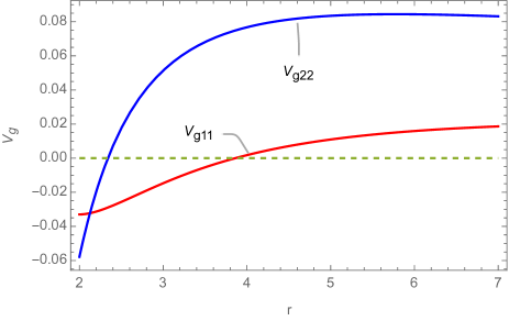
Figure 1: $V_{g11}(r)$ and $V_{g22}(r)$ for $l=1$ and $R=2$.

This fact is an indication that, for $r>2$, there are negative values of $V_{g11}$ and $V_{g22}$, so there could exist frequencies with positive imaginary part that are associated with an unstable oscillation mode. However, this analysis is not conclusive since the value of the integral in (41) could still be positive.

A suitable strategy to further the analysis of the frequencies is to apply numerical methods. Fortunately, a variety of numerical methods have been considered in order to solve this type of problems, such as continued fraction, series method, [37, 38, 29, 39], and so on, and one has the option to choose the more suitable one according to the asymptotic behavior of the potential both at spatial infinity and at the event horizon. The matrix potential ${\bf V}$, at the boundaries, behaves as the potential of Schwarzschild black hole in anti-de Sitter spacetime evaluated in the same regions. In this sense, we rely on the numerical method carried out in [29] for guidance in our case, where a similar analysis is performed. By considering a Taylor expansion of the components of field $\chi$ as follows

$$\chi_{i}=e^{-i\omega r_{*}}\sum_{n}a^{(i)}_{n}(\omega)\left(r-R\right)^{n},$$ (43)

we can substitute this into (35), and expand those differential equations in a Taylor series around the event horizon. Then, by solving the resulting algebraic equations, order by order, the coefficients $a^{(i)}_{n}(\omega)$ can be found. We observe that they only depend on the 2-dimensional vector $\mathbf{a_{0}}=\{a_{0}^{(1)},a_{0}^{(2)}\}$. In this sense, we can choose a suitable orthogonal basis for the 2-dimensional space of the initial coefficients $a_{0}^{(1)}$ and $a_{0}^{(2)}$. For each element of the basis, one constructs the $2\times 2$ matrix

$$\mathbf{S}(\omega)=\lim_{r\rightarrow\infty}\left(\begin{matrix}\chi_{1}^{(1)}&\chi_{1}^{(2)}\\ \chi_{2}^{(1)}&\chi_{2}^{(2)}\end{matrix}\right),$$ (44)

where the superscripts denote a particular vector of the basis. Certainly, $\chi_{i}^{(1)}$ corresponds to $\mathbf{a_{0}}=\{1,0\}$ and $\chi_{i}^{(2)}$ corresponds to $\mathbf{a_{0}}=\{0,1\}$ (see [39] for more specific details in the procedure). Following the line of reasoning in [39], to obtain the values of the frequencies $\omega$ it is necessary to find the zeros of (43) by imposing the condition

$$\det\mathbf{S}(\omega)=0.$$ (45)

As mentioned previously, the process indicated in (45) can be coded in Mathematica, and one can find the lowest eigenfrequencies for different values of $l$ and $R$. Indeed, taking the following variable change $r\rightarrow Rr$ in (35), we are able to find the values shown in Table 1.

$l$	$R\,\omega_{R}$	$R\,\omega_{I}$
1	$\sim$ 0	0.83
2	1.01	0.36
3	1.62	0.56
4	2.45	0.75

Table 1: Frequencies for different values of $l$.

The value $\omega_{R}$ is associated with the oscillation of the deformation while $\omega_{I}$ is related to its attenuation or increasing. Note that the imaginary part of $\omega$ is always positive for any value of $R$. These frequencies are associated with unstable deformations since the field is $\Phi\sim e^{-i\omega t}$, and this diverges when $t\rightarrow\infty$. Although a Schwarzschild four-dimensional black hole is stable in general relativity, our results show that linear instabilities are present in the embedded Schwarzschild black hole that satisfies the geodetic brane gravity equation. This kind of instabilities is also found in the study of higher-dimensional black holes, see e.g. [40].

VI Discussion

In this paper we have developed a covariant approach for the analysis of perturbations of branes governed by geodetic brane gravity through the Regge-Teitelboim geometric model, in any co-dimension.

We focus on normal deformations since they are the only ones that represent the physical perturbations. We have obtained the covariant Jacobi equations for the model, that determine the behaviour of such breathing perturbations modes $\phi^{i}$. In particular, the equations are explicitly covariant under local normal frame rotations. Within this geometric framework, some conserved geometric structures enter the game, and help to express the Jacobi equations as a set of wave-like forms from which geometric “mass” terms can be read off. There is consistency in the theory since by making the appropriate reduction for co-dimension one, results previously found are met [32].

In addition, we were able to exploit the conserved geometrical structures to construct an action, or Jacobi accessory variational principle, whose extremalization produces the Jacobi equations as its equations of motion. This action is proportional to the geometric index for the RT model. It is worth emphasizing that it is quadratic in the field modes, opening an interesting avenue in the path integral quantization of the model, that we plan to investigate in future work.

As an illustration of the general framework, using a Fronsdal scheme for a black-hole geometry, our general result has been specialized to a Schwarzschild geometry embedded in $\mathcal{M}^{6}$. A study of the Jacobi equations for this case using analytical methods is instructive, but not conclusive. On the other hand, supported by a numerical analysis, unstable small deformations are found. In this sense, it should be emphasized that our discussion of the properties of the eigenmodes $\omega$, related to the stability of this type of black holes embedded in a higher dimensional space, is neither exhaustive nor complete, but we believe that our approach opens the door to exploring the stability of interesting relativistic systems from covariant expressions obtained in the framework of extended objects. Additionally, the results presented indicate that they can be generalized to the whole class of Lovelock branes, and we consider it as a next step in the understanding of this type of geometrical models for branes.

One crucial assumption, both in physical and geometrical terms, is the embedding in a flat background spacetime of the world volume. A generalization to arbitrary background spacetimes is difficult, but for maximally symmetric ambient spacetimes like a de Sitter or anti-de Sitter background it appears to be doable. We plan to address this issue in a future communication.

Appendix A Proof for the conservation law (14).

In this appendix, we show explicitly that the tensor $\mathbb{G}_{ab}{}^{ij}$ is divergenceless. We choose to define the tensorial matrices

$$\mathbb{G}_{ab}{}^{ij}:=2\mathbb{R}_{ab}{}^{ij}-g_{ab}\mathbb{R}^{ij},$$ (46)

where

$$\mathbb{R}_{ab}{}^{ij} := K^{(i}K_{ab}{}^{j)}-K_{a}{}^{c(i}K_{bc}{}^{j)}$$ (47)

$$\mathbb{R}^{ij} := K^{i}K^{j}-K^{cd\,i}K_{cd}{}^{j}.$$ (48)

The divergence of (46) is

$$\widetilde{\nabla}^{a}\mathbb{G}_{ab}^{ij}=2\widetilde{\nabla}^{a}\mathbb{R}_{ab}^{ij}-g_{ab}\widetilde{\nabla}^{a}\mathbb{R}^{ij}.$$ (49)

On the one hand, we have for the first term

$$\widetilde{\nabla}^{a}R_{ab}^{ij} = (\widetilde{\nabla}^{a}K^{(i})\,K_{ab}{}^{j)}+(\widetilde{\nabla}^{a}K_{ab}{}^{(i})\,K^{j)}$$ (50)

$$- (\widetilde{\nabla}^{a}K_{a}{}^{c\,(i})\,K_{bc}{}^{j)}-K_{a}{}^{c\,(i}\,\widetilde{\nabla}^{a}K_{bc}^{j)}$$

$$= (\widetilde{\nabla}^{a}K^{(i})\,K_{ab}{}^{j)}+(\widetilde{\nabla}_{b}K^{(i})\,K^{j)}$$

$$- (\widetilde{\nabla}^{c}K^{(\,i})\,K_{bc}^{j)}-K_{a}{}^{c\,(i}\,\widetilde{\nabla}^{a}K_{bc}^{j)}$$

$$= (\widetilde{\nabla}_{b}K^{(i})\,K^{j)}-K_{a}{}^{c\,(i}\,\widetilde{\nabla}^{a}K_{bc}^{j)}$$

where we have used the contracted integrability condition $\widetilde{\nabla}^{a}K_{ab}^{i}=\widetilde{\nabla}_{b}K^{i}$ (Codazzi-Mainardi) to obtain the second line.

On the other hand, observe that for the second term

$$\widetilde{\nabla}_{b}\mathbb{R}^{ij}=2\left[(\widetilde{\nabla}_{b}K^{(i})\,K^{j)}-K_{a}{}^{c\,(i}\,\widetilde{\nabla}^{a}K_{bc}^{j)}\right]\,.$$ (51)

The difference between twice (50) and (51) reads

$$2\widetilde{\nabla}^{a}R_{ab}^{ij}-g_{ab}\widetilde{\nabla}^{a}R^{ij}=\widetilde{\nabla}^{a}G_{ab}^{ij}=0\,.$$ (52)

Appendix B Explicit form of transformation matrix ${\bf M}$ and effective potential ${\bf V}$.

We provide here the explicit form of the matrices appearing in (34), and write the matrices ${\bf M}$ and ${\bf V}$ in terms of them. We have

$$\begin{split}&\mathbf{A}=\left(\begin{matrix}a_{11}&a_{12}\\ a_{12}&-a_{11}\end{matrix}\right),\ \ \mathbf{B}=\left(\begin{matrix}b_{11}&b_{12}\\ b_{12}&-b_{11}\end{matrix}\right),\\ &\mathbf{C}=\left(\begin{matrix}c_{11}&c_{12}\\ c_{12}&-c_{11}-\frac{6R^{2}}{r^{6}}\end{matrix}\right),\ \ \mathbf{D}=\left(\begin{matrix}d_{11}&d_{12}\\ d_{12}&-d_{11}\end{matrix}\right).\end{split}$$ (53)

Notice that ${\bf A}$, ${\bf B}$ and ${\bf D}$ are traceless symmetric matrices while ${\bf C}$ is not. In fact, this is responsible for not being able to decouple the system of equations (34). The explicit components of these matrices are

$$\begin{split}&a_{11}=\frac{2R\left(r^{3}-R^{3}\right)}{r^{3}\left(r^{3}+r^{2}R+rR^{2}+R^{3}\right)},\\ &a_{12}=-\frac{(r-R)(r^{3}+r^{2}R+rR^{2}-R^{3})\sqrt{r^{3}R(r^{2}+rR+R^{2})}}{r^{5}R(r^{3}+r^{2}R+rR^{2}+R^{3})},\\ &b_{11}=\frac{2R\left(-r^{6}+r^{4}R^{2}+6r^{3}R^{3}+3r^{2}R^{4}+2rR^{5}+R^{6}\right)}{r^{4}\left(r^{3}+r^{2}R+rR^{2}+R^{3}\right)^{2}},\\ &b_{12}=\frac{-r^{9}-3r^{8}R-6r^{7}R^{2}-22r^{6}R^{3}-20r^{5}R^{4}-16r^{4}R^{5}+6r^{3}R^{6}+6r^{2}R^{7}+5rR^{8}+3R^{9}}{2r^{3}\sqrt{r^{3}R\left(r^{2}+rR+R^{2}\right)}\left(r^{3}+r^{2}R+rR^{2}+R^{3}\right)^{2}},\\ &c_{11}=l(l+1)\frac{R(r-R)\left(r^{2}+2rR+3R^{2}\right)}{r^{5}\left(r^{3}+r^{2}R+rR^{2}+R^{3}\right)}-\frac{R^{2}\left(9r^{9}+27r^{8}R+54r^{7}R^{2}+42r^{6}R^{3}+17r^{5}R^{4}-21r^{4}R^{5}+4rR^{8}+12R^{9}\right)}{2r^{6}\left(r^{3}+r^{2}R+rR^{2}+R^{3}\right)^{3}},\\ &c_{12}=l(l+1)\frac{\sqrt{\frac{r^{3}R}{r^{2}+rR+R^{2}}}\left(r^{6}+2r^{5}R+3r^{4}R^{2}+16r^{3}R^{3}+15r^{2}R^{4}+14rR^{5}-3R^{6}\right)}{4r^{7}R\left(r^{3}+r^{2}R+rR^{2}+R^{3}\right)}\\ &-\frac{R\left(3r^{11}+12r^{10}R+30r^{9}R^{2}+90r^{8}R^{3}+182r^{7}R^{4}+296r^{6}R^{5}+254r^{5}R^{6}+150r^{4}R^{7}-5r^{3}R^{8}-56r^{2}R^{9}-56rR^{10}-36R^{11}\right)}{4r^{11/2}\sqrt{R\left(r^{2}+rR+R^{2}\right)}\left(r^{3}+r^{2}R+rR^{2}+R^{3}\right)^{3}},\\ &d_{11}=-\frac{6R^{4}}{r^{6}-r^{2}R^{4}},\\ &d_{12}=\frac{3R^{2}\left(r^{3}+r^{2}R+rR^{2}-R^{3}\right)\sqrt{r^{3}R\left(r^{2}+rR+R^{2}\right)}}{(r^{7}-r^{4}R^{3})\left(r^{3}+r^{2}R+rR^{2}+R^{3}\right)}.\end{split}$$ (54)

On account of the definition

$${\bf h}:=-\left(\frac{{\bf D}^{-1}{\bf B}}{f_{g}}+{\bf I}\frac{df_{g}}{dr}\right),$$ (55)

where ${\bf I}$ denotes the $2\times 2$ unit matrix, we find that the matrix $\mathbf{M}$ can be written as

$$\mathbf{M}=\exp\left(-\frac{1}{2}\int\frac{{\bf h}}{f_{g}}dr\right).$$ (56)

In the same way, the potential matrix ${\bf V}$ in terms of these matrices, becomes

$${\bf V}=\frac{f_{g}}{2}\frac{d{\bf h}}{dr}+\frac{1}{4}{\bf h}^{2}+{\bf M}^{-1}{\bf D}^{-1}{\bf C}{\bf M}.$$ (57)

References

- Regge and Teitelboim [1977] T. Regge and C. Teitelboim, General relativity à la string: a progress report, in Proceddings of the Marcel Grossman Meeting, Trieste, Italy (1975), edited by R. Ruffini (North-Holland, Amsterdam, 1977) 77 (1977).
- Goon et al. [2011] G. L. Goon, K. Hinterbichler, and M. Trodden, New class of effective field theories from embedded branes, Phys. Rev. Lett. 106, 231102 (2011).
- Cruz and Rojas [2013] M. Cruz and E. Rojas, Born–infeld extension of Lovelock brane gravity, Class. Quant. Grav. 30, 115012 (2013).
- Maia [1986] M. Maia, On Kaluza-Klein relativity, General Relativity and Gravitation 18, 695 (1986).
- Pavšič [1986] M. Pavšič, Einstein’s gravity from a first order Lagrangian in an embedding space, Phys. Lett. A 116, 1 (1986).
- Tapia [1989] V. Tapia, Gravitation à la string, Class. Quant. Grav. 6, L49 (1989).
- Davidson et al. [2001] A. Davidson, D. Karasik, and Y. Lederer, Cold dark matter from dark energy, arXiv preprint gr-qc/0111107 (2001).
- Copeland et al. [2006] E. J. Copeland, M. Sami, and S. Tsujikawa, Dynamics of dark energy, International Journal of Modern Physics D 15, 1753 (2006).
- Bertone and Hooper [2018] G. Bertone and D. Hooper, History of dark matter, Reviews of Modern Physics 90, 045002 (2018).
- Sotiriou and Faraoni [2010] T. P. Sotiriou and V. Faraoni, R theories of gravity, Reviews of Modern Physics 82, 451 (2010).
- De Felice and Tsujikawa [2010] A. De Felice and S. Tsujikawa, R theories, Living Rev. Relativ. 13, 1 (2010).
- Nojiri et al. [2017] S. Nojiri, S. D. Odintsov, and V. K. Oikonomou, Modified gravity theories on a nutshell: inflation, bounce and late-time evolution, Phys. Rept. 692, 1 (2017).
- Arkani-Hamed et al. [1998] N. Arkani-Hamed, S. Dimopoulos, and G. Dvali, The hierarchy problem and new dimensions at a millimeter, Phys. Lett. B 429, 263 (1998).
- Randall and Sundrum [1999] L. Randall and R. Sundrum, Large mass hierarchy from a small extra dimension, Phys. Rev. Lett. 83, 3370 (1999).
- Maartens and Koyama [2010] R. Maartens and K. Koyama, Brane-world gravity, Living Rev. Relativ. 13, 5 (2010).
- Davidson and Karasik [1998] A. Davidson and D. Karasik, Quantum gravity of a brane-like universe, Modern Physics Letters A 13, 2187 (1998).
- Karasik and Davidson [2003] D. Karasik and A. Davidson, Geodetic brane gravity, Phys. Rev. D 67, 064012 (2003).
- Polyakov [1986] A. Polyakov, Fine structure of strings, Nuclear Physics B 268, 406 (1986).
- Carter and Gregory [1995] B. Carter and R. Gregory, Curvature corrections to dynamics of domain walls, Phys. Rev. D 51, 5839 (1995).
- Janet [1926] M. Janet, Sur la possibilité de plonger un espace riemannien donné dans un espace euclidien, Ann. Soc. Pol. Math 5, 38 (1926).
- Cartan [1927] É. Cartan, Sur la possibilité de plonger un espace riemannien donné dans un espace euclidien, Ann. Soc. Polon. Math. 6, 1 (1927).
- Friedman [1961] A. Friedman, Local isometric imbedding of riemannian manifolds with indefinite metrics, J. of Mathematics and Mechanics 10, 625 (1961).
- Rosen [1965] J. Rosen, Embedding of various relativistic riemannian spaces in pseudo-euclidean spaces, Reviews of Modern Physics 37, 204 (1965).
- Paston and Sheykin [2012] S. Paston and A. Sheykin, Embeddings for the Schwarzschild metric: classification and new results, Class. Quant. Grav. 29, 095022 (2012).
- Wald [2010] R. M. Wald, General relativity (University of Chicago press, 2010).
- Kot [2014] M. Kot, A first course in the calculus of variations, Vol. 72 (American Mathematical Society, 2014).
- Fomenko and Tuzhilin [2005] A. T. Fomenko and A. A. Tuzhilin, Elements of the geometry and topology of minimal surfaces in three-dimensional space, Vol. 93 (American Mathematical Soc., 2005).
- Colding and Minicozzi [2011] T. H. Colding and W. P. Minicozzi, A course in minimal surfaces, Vol. 121 (American Mathematical Soc., 2011).
- Horowitz and Hubeny [2000] G. T. Horowitz and V. E. Hubeny, Quasinormal modes of ads black holes and the approach to thermal equilibrium, Phys. Rev. D 62, 024027 (2000).
- Chamblin et al. [2000] A. Chamblin, S. Hawking, and H. Reall, Brane-world black holes, Phys. Rev. D 61, 065007 (2000).
- Capovilla and Guven [1995] R. Capovilla and J. Guven, Geometry of deformations of relativistic membranes, Phys. Rev. D 51, 6736 (1995).
- Bagatella-Flores et al. [2016] N. Bagatella-Flores, C. Campuzano, M. Cruz, and E. Rojas, Covariant approach of perturbations in Lovelock type brane gravity, Class. Quant. Grav. 33, 245012 (2016).
- Zinn-Justin [2021] J. Zinn-Justin, Quantum field theory and critical phenomena, Vol. 171 (Oxford university press, 2021).
- Guven [1993] J. Guven, Covariant perturbations of domain walls in curved spacetime, Phys. Rev. D 48, 4604 (1993).
- Fronsdal [1959] C. Fronsdal, Completion and embedding of the Schwarzschild solution, Phys. Rev. 116, 778 (1959).
- Davidson and Paz [2000] A. Davidson and U. Paz, Extensible embeddings of black-hole geometries, Foundations of Physics 30, 785 (2000).
- Ferrari et al. [2007] V. Ferrari, L. Gualtieri, and S. Marassi, New approach to the study of quasinormal modes of rotating stars, Phys. Rev. D 76, 104033 (2007).
- Pani et al. [2012] P. Pani, V. Cardoso, L. Gualtieri, E. Berti, and A. Ishibashi, Perturbations of slowly rotating black holes: massive vector fields in the Kerr metric, Phys. Rev. D 86, 104017 (2012).
- Pani [2013] P. Pani, Advanced methods in black-hole perturbation theory, International Journal of Modern Physics A 28, 1340018 (2013).
- Gregory and Laflamme [1993] R. Gregory and R. Laflamme, Black strings and p-branes are unstable, Phys. Rev. Lett. 70, 2837 (1993).