Electron scattering of mass-inverted in graphene quantum dots

Abstract

We study the scattering of Dirac electrons of circular graphene quantum dot with mass-inverted subject to an electrostatic potential. The obtained solutions of energy spectrum are used to determine the scattering coefficients at the interface of the two regions. Using the asymptotic solutions at large arguments, we explicitly determine the radial component of reflected current density and the scattering efficiency. It is found that the presence of a mass term outside in addition to another one inside the quantum dot strongly affects the scattering of electrons. In particular, a non-null square modulus of the scattering coefficient is found at zero energy.

I Introduction

Graphene [1] has incredible transport properties [2, 3] letting it to be a potential candidate for technological applications in the future [4]. The interaction of electrons moving around the carbon atoms with the periodic potential of the graphene honeycomb lattice generates relativistic massless Dirac fermions showing a linear energy dispersion [6, 5]. These fermions have been found to travel with a speed much faster than that of electrons in semiconductors [7, 8]. Additionally, graphene remains capable of conducting electricity even at the limit of nominal carrier concentration, meaning that it never stops conducting. In contrast, Klein tunneling (full transmission) provides a window path for graphene electrons that limits the efficiency of electrostatic confinement [5, 9]. Consequently, the fabrication of graphene-based materials will remain a great challenge for various flexible device applications. One way to overcome such situation is to confine the electrons in graphene using different techniques and then the realization of graphene quantum dots (GQDs) can offer an alternative solution.

GQDs are made up of a single atomic layer of nano-sized graphite. They have many of the same properties as graphene, including a large surface area, a big diameter, and superior surface grafting employing $\pi-\pi$ conjugation and surface groups [10, 11]. Recently, QDGs have been extensively discussed both theoretically [12, 13, 14, 15, 16, 17, 18] and experimentally [19, 20, 21]. Different methods have been proposed to confine electrons in graphene and then generate interesting systems based-graphene. These concern for instance employing thin single-layer graphene strips [12, 14] or nonuniform magnetic fields [22]. Another way to use low-disorder graphene crystallographically matched to hexagonal boron nitride substrate and electrostatic confinement [23]. It is found that GQDs strongly depend on their sizes, shapes and nature of edges [6]. GQDs can be applied in the spin qubits and quantum information storage [5, 13]. Also they can be used in the fields of bio-imaging, sensors, catalysis, photovoltaic devices, superconductors and so on [24].

On the other hand, systems made of gapped graphene with different band gaps can be used to host topologically protected metallic channels in amazing ways. As a result, due to periodic interlayer interaction with substrates, different band gaps can be generated in graphene [25, 26, 27]. In this context, the helical states around a mass-inverted quantum dot in graphene was studied in [28]. To introduce a mass-inverted quantum dot a heterojunction between two separate mass domains is used in similar way to the domain wall in bilayer graphene. It was showed that the eigenstates are doubly degenerate, with each state propagating in opposing directions, preserving graphene’s time-reversal symmetry.

Motivated by the results mentioned above and especially [28], we study the scattering of electrons in circular graphene quantum dot with mass-inverted terms through an electrostatic potential. We analytically determine the solutions of energy spectrum by solving Dirac equation. In some limit, we explicitly obtain the radial component of density current associated to reflected wave. This is used to compute the corresponding scattering efficiency in terms of the gaps outside and inside the quantum dot. The main characteristics of these quantities are studied in relation to the physical parameters of our system. For this, we identify different scattering regimes as a function of the radius, applied potential, two gaps and incident energy. As results, we show that the energy gap outside the quantum dot strongly affects the scattering of electrons in graphene.

The present paper is organized as follows. In section II, we set a theoretical model describing our system made of circular graphene quantum dot with two gaps. Subsequently, we establish the spinor solutions of the Dirac equation for the two regions. We use the continuity of the wave functions at the boundary to explicitly determine physical quantities in section III. We numerically analyze and discuss the main results under various conditions in section IV. Finally, we conclude our work.

II Theoretical model

To achieve our goal, let us consider graphene quantum dot of radius $r_{0}$ with two mass terms $\Delta(r)$ and electrostatic potential $V(r)$. Mathematically, we have

$$\Delta(r)=\left\{\begin{array}[]{ll}\Delta_{1},&r>r_{0}\\ \Delta_{2},&r\leq r_{0}\end{array}\right.,\qquad V(r)=\left\{\begin{array}[]{ll}0,&r>r_{0}\\ V,&r\leq r_{0}\end{array}\right.$$ (1)

and schematically we represent our system in Figure 1.

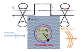
Figure 1: (color online) Dirac electrons propagating in a gapped graphene subject to the potential barrier in a circular quantum dot of radius $r_{0}$. Here the incident and reflected electron waves reside in the conduction band with gap $\Delta_{1}$, while the transmitted wave inside the dot corresponds to a state in the valence band with gap $\Delta_{2}$.

The single-valley Hamiltonian describing circular graphene quantum dot can be written as (in the system unit $\hbar=\nu_{F}=1$)

$$H=-i\vec{\nabla}\cdot\vec{\sigma}+V(r)\mathbb{I}_{2}+\Delta{(r)}\sigma_{z}$$ (2)

where $\vec{\sigma}=(\sigma_{x},\sigma_{y},\sigma_{z})$ are the Pauli matrices and $\mathbb{I}_{2}$ is the unit matrix. In polar coordinates $(r,\theta)$ and by introducing the potentials and operators

$$W_{\pm}=V\pm\Delta_{1}\pm\Delta_{2}$$ (3)

$$\partial_{\pm}=e^{\mp i\theta}\left(-i{\partial_{r}}\pm\dfrac{1}{r}{\partial\theta}\right)$$ (4)

we map (2) as

$$H=\begin{pmatrix}W_{+}&\partial_{+}\\ \partial_{-}&W_{-}\end{pmatrix}.$$ (5)

One can show that the commutation relation $[H,J_{z}]$ is fulfilled by the total momentum operator $J_{z}=L_{z}+\frac{1}{2}\sigma_{z}$ and (5). This provides the separability of the eigenspinors $\psi_{m}(r,\theta)$ of the Hamiltonian (5) into radial $R^{\pm}(r)$ and angular $\chi^{\pm}(\theta)$ parts

$$\psi_{m}{(r,\theta)}=\begin{pmatrix}R^{+}_{m}(r)\chi^{+}(\theta)\\ R^{-}_{m+1}(r)\chi^{-}(\theta)\end{pmatrix}$$ (6)

where the eigenstates of $J_{z}$ are

$$\chi^{+}(\theta)=\dfrac{e^{im\theta}}{\sqrt{2\pi}}\begin{pmatrix}1\\ 0\end{pmatrix},\qquad\chi^{-}(\theta)=\dfrac{e^{i(m+1)\theta}}{\sqrt{2\pi}}\begin{pmatrix}0\\ 1\end{pmatrix}$$ (7)

and $m=0,\pm 1,\pm 2,\cdots$ being the angular momentum quantum number.

In order to get the solutions of the energy spectrum, we complete the derivation of the eigenspinors by determining the radial parts. It can be achieved by solving $H\psi_{m}{(r,\theta)}=E\psi_{m}{(r,\theta)}$ in outside $r>r_{0}$ and inside $r\leq r_{0}$ regions of the quantum dot, see Figure 1. Indeed, for $r>r_{0}$, we show that the radial components $R^{+}_{m}(r)$ and $R^{-}_{m+1}(r)$ satisfy two coupled differential equations

$$\left(-i{\partial_{r}}+i\frac{m}{r}\right)R^{+}_{m}=(E+\Delta_{1})R^{-}_{m+1}$$ (8)

$$\left(-i{\partial_{r}}-i\frac{m+1}{r}\right)R^{-}_{m+1}=(E-\Delta_{1})R^{+}_{m}.$$ (9)

By injecting (8) into (9) we find a second differential equation

$$\left(r^{2}{\partial_{r}^{2}}+r{\partial_{r}}+r^{2}k_{1}^{2}-m^{2}\right)R^{+}_{m}(r)=0$$ (10)

from which we find the Bessel functions $J_{m}(k_{1}r)$ as solution and set the parameter

$$k_{1}=\sqrt{{E^{2}}-\Delta_{1}^{2}}.$$ (11)

It is convenient to write the incident plane wave as

$$\psi_{i}{(r,\theta)}=\dfrac{1}{\sqrt{2}}\sum_{m}{i^{m}}J_{m}(k_{1}r)e^{im\theta}\begin{pmatrix}1\\ 1\end{pmatrix}.$$ (12)

With this, we end up with the incident and reflected spinors

$$\psi_{i}{(r,\theta)}= \sqrt{\pi}\sum_{m}{i^{m+1}}\left[-iJ_{m}(k_{1}r)\chi^{+}(\theta)+\mu_{1}J_{m+1}(k_{1}r)\chi^{-}(\theta)\right]$$ (13)

$$\psi_{r}{(r,\theta)}= \sqrt{\pi}\sum_{m}{i^{m+1}}a_{m}\left[-iH^{(1)}_{m}(k_{1}r)\chi^{+}(\theta)+\mu_{1}H^{(1)}_{m+1}(k_{1}r)\chi^{-}(\theta)\right]$$ (14)

where $H^{(1)}_{m}(k_{1}r)$ is the Hankel function of the first kind, $a_{m}$ are the scattering coefficients. Here we have defined dimensionless parameter

$$\mu_{1}=\sqrt{\frac{E-\Delta_{1}}{E+\Delta_{1}}}$$ (15)

in terms of the first energy gap $\Delta_{1}$ and it reduces to one for $\Delta_{1}=0$.

Now we consider the second region $r\leq r_{0}$ with the potential $V$ and energy gap $\Delta_{2}$. As a result, we find the following equations

$$\left(-i{\partial_{r}}+i\frac{m}{r}\right)R^{+}_{m}=(E-V+\Delta_{2})R^{-}_{m+1}$$ (16)

$$\left(-i{\partial_{r}}-i\frac{m+1}{r}\right)R^{-}_{m+1}=(E-V-\Delta_{2})R^{+}_{m}$$ (17)

giving rise to

$$(r^{2}{\partial_{r}^{2}}+r{\partial_{r}}+r^{2}k_{2}^{2}-m^{2})R^{+}_{m}=0$$ (18)

and we have set

$$k_{2}=\sqrt{(E-V)^{2}-\Delta_{2}^{2}}.$$ (19)

From (18) we derive the transmitted spinor solution

$$\psi_{t}{(r,\theta)}=\sqrt{\pi}\sum_{m}{i^{m+1}}b_{m}\left[-iJ_{m}(k_{2}r)\chi^{+}(\theta)+\mu_{2}J_{m+1}(k_{2}r)\chi^{-}(\theta)\right]$$

where $b_{m}$ are the scattering coefficients and

$$\mu_{2}=\sqrt{\frac{E-V-\Delta_{2}}{E-V+\Delta_{2}}}.$$ (20)

In the next, we will see how the above results can be used to study the scattering of Dirac electrons in our system with the presence of two mass terms.

III Scattering problem

To study the scattering problem associated our system, in the first stage we determine the scattering coefficients $a_{m}$ and $b_{m}$. To this end, we use of the boundary condition at interface $r=r_{0}$ to write

$$\psi_{i}{(r_{0})}+\psi_{r}{(r_{0})}=\psi_{t}{(r_{0})}.$$ (21)

After substitution, we establish two relations between Bessel and Hankel functions

$$J_{m}(k_{1}r_{0})+a_{m}H^{(1)}_{m}(k_{1}r_{0})=b_{m}J_{m}(k_{2}r_{0})$$ (22)

$$\mu_{1}J_{m+1}(k_{1}r_{0})+\mu_{1}a_{m}H^{(1)}_{m+1}(k_{1}r_{0})=\mu_{2}b_{m}J_{m+1}(k_{2}r_{0})$$ (23)

which can be solved to obtain the scattering coefficients

$$a_{m}=\frac{{\mu_{2}J_{m}(k_{1}r_{0})J_{m+1}(k_{2}r_{0})-\mu_{1}J_{m}(k_{2}r_{0})J_{m+1}(k_{1}r_{0})}}{\mu_{1}J_{m}(k_{1}r_{0})H^{(1)}_{m+1}(k_{1}r_{0})-\mu_{2}J_{m+1}(k_{2}r_{0})H^{(1)}_{m}(k_{1}r_{0})}$$ (24)

$$b_{m}=\frac{{\mu_{1}J_{m}(k_{1}r_{0})H^{(1)}_{m+1}(k_{1}r_{0})-\mu_{1}J_{m+1}(k_{1}r_{0})H^{(1)}_{m}(k_{1}r_{0})}}{\mu_{1}J_{m}(k_{1}r_{0})H^{(1)}_{m+1}(k_{1}r_{0})-\mu_{2}J_{m+1}(k_{2}r_{0})H^{(1)}_{m}(k_{1}r_{0})}.$$ (25)

At this level, we compute the radial component of current density corresponding to our system. For this, we use the Hamiltonian (1) to obtain the current density

$$\vec{j}=\psi^{\dagger}\vec{\sigma}\psi$$ (26)

where inside the quantum dot $\psi=\psi_{t}$ and outside $\psi=\psi_{i}+\psi_{r}$. From the projection

$$j_{r}=\vec{j}\cdot\vec{e}_{r}$$ (27)

one obtains

$$j_{r}=\psi^{\dagger}\begin{pmatrix}0&\cos{\theta}-i\sin{\theta}\\ \cos{\theta}+i\sin{\theta}&0\end{pmatrix}\psi.$$ (28)

As far as the reflected wave (14) is concerned, we get

$$j^{r}_{r}=\dfrac{1}{2}\sum_{m=0}^{\infty}A_{m}(k_{1}r)\begin{pmatrix}0&{e^{-i\theta}}\\ e^{i\theta}&0\end{pmatrix}\sum_{m=0}^{\infty}B_{m}(k_{1}r)$$ (29)

such that

$$A_{m}(k_{1}r)=(-i)^{m+1}\left[iH^{(1)^{*}}_{m}(k_{1}r)\begin{pmatrix}a^{*}_{m}e^{im\theta}&a^{*}_{-m-1}e^{-im\theta}\end{pmatrix}+\mu_{1}H^{(1)}_{m+1}(k_{1}r)\begin{pmatrix}a^{*}_{-m-1}e^{i(m+1)\theta}&a^{*}_{m}e^{-i(m+1)\theta}\end{pmatrix}\right]$$ (30)

$$B_{m}(k_{1}r)=(-i)^{m+1}\left[iH^{(1)}_{m}(k_{1}r)\begin{pmatrix}a^{*}_{m}e^{-im\theta}\\ a^{*}_{-m-1}e^{im\theta}\end{pmatrix}+\mu_{1}H^{(1)^{*}}_{m+1}(k_{1}r)\begin{pmatrix}a^{*}_{-(m+1)}e^{i(m+1)\theta}\\ a^{*}_{m}e^{-i(m+1)\theta}\end{pmatrix}\right].$$ (31)

To illustrate our results and give a better understanding let us consider the asymptotic behavior of the Hankel function for large argument $k_{1}r\gg 1$. With this we will be able to explicitly establish analytical results of the above quantities. Then in such limit, one can use the approximate function

$$H_{m}(k_{1}r)\simeq\sqrt{\dfrac{2}{\pi k_{1}r}}e^{(k_{1}r-\frac{m\pi}{2}-\frac{\pi}{4})}$$ (32)

which can be injected into (30-31) to approximate the radial component (29) by

$$j^{r}_{r}=\frac{2}{\pi k_{1}r}\sum_{m=0}^{\infty}|c_{m}|^{2}\left(\cos[(2m+1)\theta](1+\mu_{1}^{2})+2\mu_{1}\right)$$ (33)

where the square modulus of the scattering coefficients

$$|c_{m}|^{2}=\frac{1}{2}(|a_{m}|^{2}+|a_{-(m+1)}|^{2})$$ (34)

are given in terms of $a_{m}$ (24). Actually (33-34) show a strong dependence on the energy gap $\Delta_{1}$ outside the quantum dot that is not the case for analogue results obtained in [18]. As a consequence, we will study the rule will be played by $\Delta_{1}$ to affect the scattering problem of our system.

Let us analyze other physical quantities related to the radial current for the reflected wave (33). Indeed, the scattering cross-section $\sigma$ is defined by

$$\sigma=\frac{I^{r}_{r}}{(I_{i}/A_{u})}$$ (35)

such that the total reflected flux per unit area $I^{r}_{r}$ can be calculated by integrating (33)

$$I^{r}_{r}=\int^{2\pi}_{0}j^{r}_{r}(\theta)rd\theta$$ (36)

and as a result we find

$$I^{r}_{r}=\frac{8}{E+\Delta_{1}}\sum_{m=0}^{\infty}|c_{m}|^{2}$$ (37)

while for the incident wave (12) the ratio $I_{i}/A_{u}$ is just the unit and therefore the cross-section reduces to $I^{r}_{r}$, i.e. $\sigma=I^{r}_{r}$.

To go deeply in the study of the scattering problem for Dirac electron in graphene circular quantum dot, we consider the scattering efficiency $Q$. It is defined by the ratio between the scattering cross-section and the geometric cross-section

$$Q=\frac{\sigma}{2r_{0}}$$ (38)

and then using (37) to get

$$Q=\frac{4}{r_{0}(E+\Delta_{1})}\sum_{m=0}^{\infty}|c_{m}|^{2}.$$ (39)

We emphasis that in the case $\Delta_{1}=0$ our results reduce to those obtained in [18]. We will numerically show how the presence of $\Delta_{1}$ will affect the scattering problem.

IV Results and discussions

We proceed a numerical analysis by considering various conditions of the physical parameters to underline the main features of our system. Indeed, Figure 2 represents the scattering efficiency $Q$ as a function of the quantum dot radius $r_{0}$. Here we choose $V=1$ and $\Delta_{2}=0.2$, with (a,b,c): $\Delta_{1}=0.5$ and (d,e,f): $\Delta_{1}=0.7$. Three scattering regimes of the incident energy $E$ are considered. Figures 2(a,d) show the results for the regime $E<W_{-}$ outside the quantum dot. We notice that $Q$ increases linearly for small radius, but when the radius reaches a certain value $Q$ begins to change by showing a oscillatory behavior until reaches a maximum. By increasing further $r_{0}$, we observe a decrease on the oscillations shape of $Q$. We notice that $Q$ is very sensitive to the incident energy $E$ because it decreases when $E$ increases. In addition for $\Delta_{1}=0.5$ in Figure 2(a) there is a maximum value $Q=4$ when $r_{0}$ tends to $4$. While for $\Delta_{1}=0.7$ in Figure 2(d) the maximum value is $Q=3$ when $r_{0}$ tends towards $8$. The period of oscillations corresponding to $\Delta_{1}=0.5$ is small compared to the case $\Delta_{1}=0.7$. Figures 2(b,e) show the behavior of $Q$ for the electronic state inside the quantum dot $W_{-}<E<W_{+}$. It is clearly seen that $Q$ increases linearly up to a certain value of $r_{0}$, then $Q$ changes in oscillatory shape with different amplitudes depending on the incident energy $E$. In fact, for $\Delta_{1}=0.5$ when $r_{0}$ tends to $6$ and for $\Delta_{1}=0.7$ when $r_{0}$ tends to $10$ these amplitudes changes inversely with incident energy values, and afterword the oscillations begin to be damped. The last regime of energy $E>W_{+}$ is presented in Figures 2(c,f). As one sees for small radius, $Q$ changes in a linear manner and its values are very close to each other regardless of the incident energy. However, when the radius reaches a certain value, $Q$ changes by oscillating with decreasing amplitudes until a certain value of $r_{0}$. These results show the influence of the gap $\Delta_{1}$ on the scattering efficiency $Q$.

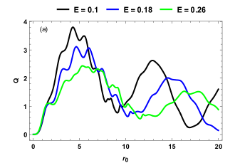
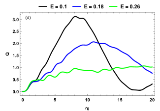
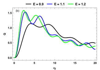
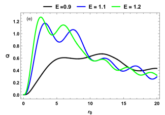
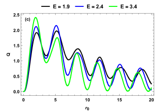
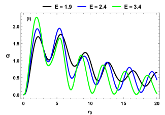
Figure 2: (color online) The scattering efficiency ${Q}$ versus the quantum dot radius $r_{0}$ for $\Delta_{2}=0.2$ and $V=1$. Three regimes of the incident energy are considered (a,d): $E<W_{-}$, (b,e): $W_{-}<E<W_{+}$, (c,f): $E>W_{+}$. Here (a,b,c): $\Delta_{1}=0.5$ and (d,e,f): $\Delta_{1}=0.7$.

We plot in Figure 3 the scattering efficiency $Q$ as a function of the incident energy $E$ for $V=1$, $\Delta_{2}=0.2$, two values $\Delta_{1}=0.5,0.9$ and different sizes of the quantum dot. For small values of $r_{0}$ in Figures 3(a,c) $Q$ takes 4 as maximum value for $E=0$ and $\Delta_{1}=0.5$. It decreases rapidly until it approaches zero at $E=\Delta_{1}=0.5$. When the energy increases $Q$ gradually increases by oscillating to reach constant values. For $\Delta_{1}=0.9$ we observe that $Q$ is minimal at $E=0$ but it reaches the maximum value $1.2$ by increasing $E$. Later on it decreases to approaches zero at $E=\Delta_{1}=0.9$ and after that both of them increase. For large radius $r_{0}$ in Figures 3(b,d) $Q$ is not zero for $E=0$ and shows large maxima. The maximum value of $Q$ decreases when $r_{0}$ increases then decreases towards a value close to zero for $E=\Delta_{1}=0.5$. By increasing $E$, $Q$ takes constant values and strongly depends on $r_{0}$. As for $\Delta_{1}=0.9$, $Q$ has a minimum value at $E=0$ and reaches $1.8$ as maximum when $E$ increases. It decreases to approaches zero at $E=\Delta_{1}=0.9$ but once $E$ increases we observe an increase of $Q$ for both sizes $r_{0}=5.75,6.25$.

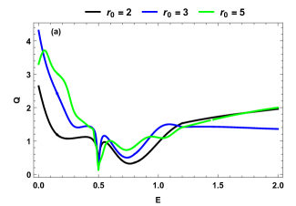
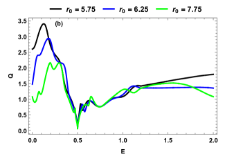
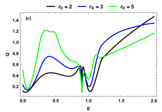
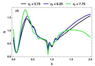
Figure 3: (color online) The scattering efficiency $Q$ versus the incident energy $E$ for $\Delta_{2}=0.2$ and $V=1$. Different sizes of the quantum dot are considered. Here (a,b): $\Delta_{1}=0.5$ and (c,d): $\Delta_{1}=0.9$.

In order to show how the potential $V$ affects the scattering we represent in Figure 4 the scattering efficiency $Q$ as a function of the incident energy $E$ for $\Delta_{2}=0.2$ and $r_{0}=3$ with (a): $\Delta_{1}=0.5$ and (b): $\Delta_{1}=0.9$. It is clearly seen that when $E$ closes to zero, $Q$ is not null and its values are strongly depending on both parameters $V$ and $\Delta_{1}$. Moreover, as long as $E$ increases we observe that $Q$ decreases towards $\Delta_{1}$ by showing small oscillations with different amplitudes. Afterwords, one sees that $Q$ starts to increase by increasing $E$ for large potential $V$. An interesting conclusion can be emphasized such that for $E<\Delta_{1}=0.5$ in Figure 4, $Q$ takes small values compared to the case $E<\Delta_{1}=0.9$ in Figure 4b. However, for the case $E>\Delta_{1}=0.5$ and $E>\Delta_{1}=0.9$ we observe the opposite behavior.

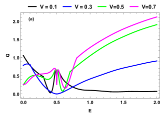
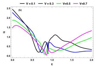
Figure 4: (color online) The scattering efficiency $Q$ versus the incident energy $E$ for $\Delta_{2}=0.2$ and $r_{0}=3$. Different values of the potential $V$ are considered. Here (a): $\Delta_{1}=0.5$ and (b): $\Delta_{1}=0.9$.

Figure 5 represents the scattering efficiency $Q$ as a function of the incident energy $E$ for different values of energy gap $\Delta_{2}$ inside the quantum dot with $V=1$ and $r_{0}=2$. Here we choose two values such that (a): $\Delta_{1}=0.5$ and (b): $\Delta_{1}=0.9$. It is clearly seen that $Q$ is not null for $E=0$. Under the increase of $E$ we observe that $Q$ decreases by approaching zero at the point $E=\Delta_{1}=0.5$ as shown in Figure 5a. Afterward, $Q$ oscillates to reach constant values depending on $\Delta_{2}$. Now in Figure 5b for $\Delta_{1}=0.9$ one sees that $Q$ shows mostly the same behavior regardless the value of $\Delta_{2}$ in the interval $0<E<\Delta_{1}=0.9$ except that it increases. Whereas for $E>\Delta_{1}=0.9$ we observe that $Q$ presents some oscillations and afterward it increase.

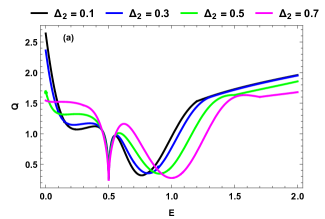
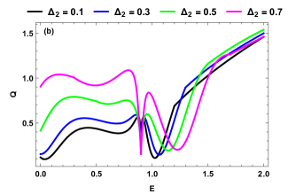
Figure 5: (color online) The scattering efficiency $Q$ versus the incident energy $E$ for $V=1$ and $r_{0}=2$. Different values of the gap inside quantum dot $\Delta_{2}$ are considered. Here, (a): $\Delta_{1}=0.5$ and (b): $\Delta_{1}=0.9$.

We show the influence of the gap outside quantum dot $\Delta_{1}$ on the scattering efficiency in Figure 6. It is clearly seen that $Q$ presents different behavior compared to that for the energy gap $\Delta_{2}$ inside the quantum dot (Figure 5). As a result, we observe that $Q$ is showing maximum values only for small energies and gaps $\Delta_{1}$. In contrast, when $E$ increases $Q$ becomes mostly weak and it goes towards to a constant regardless the values taken by $\Delta_{1}$. Another remark is that the behavior of $Q$ decreases as long as $\Delta_{2}$ increases.

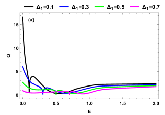
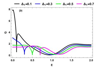
Figure 6: (color online) The scattering efficiency $Q$ versus the incident energy $E$ for $V=1$, $r_{0}=2$ and $\Delta_{2}=0.2$. Different values of of the gap outside quantum dot $\Delta_{1}$ are considered. Here, (a): $\Delta_{2}=0.2$ and (b): $\Delta_{2}=0.7$.

In Figure 7 we plot the square modulus of the scattering coefficients $|c_{m}|^{2}$ ($m=0,1,2,3$) as a function of the incident energy $E$ for $V=1$, $\Delta_{2}=0.2$ and different sizes of quantum dot, with (a): $\Delta_{1}=0.1$ and (b): $\Delta_{1}=0.9$. As a result, we observe that $|c_{m}|^{2}$ strongly depends on the size of quantum dots. It shows oscillatory behaviors with different amplitudes as long as $r_{0}$ increase. For $E<\Delta_{1}$ and small $r_{0}$, $|c_{m}|^{2}$ decrease and increase for large $r_{0}$. At the point $E=\Delta_{1}$, $|c_{m}|^{2}$ show minimum peaks. Compared to the results for one energy gap inside the quantum dots [18], we stress that the presence of a gap outside gives a non-null square modulus of the diffusion coefficient for both cases $E=0$ and $E<\Delta_{1}$. Just after $E=\Delta_{1}$, it is clearly seen that $|c_{m}|^{2}$ show oscillatory behaviors.

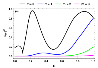
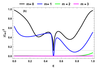
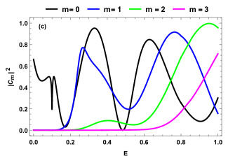
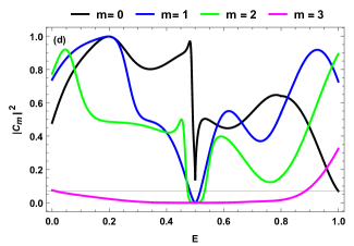
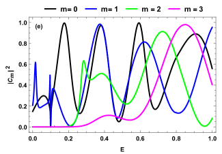
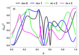
Figure 7: (color online) The square modulus of the scattering coefficients $|c_{m}|^{2}$ ($m=0,1,2,3$) versus the incident energy $E$ for $\Delta_{2}=0.2$ and $V=1$ with different sizes of quantum dot (a,b): $r_{0}$ =3, (c,d): $r_{0}$ =5, (e,f): $r_{0}$ =7. Here (a,b,c): $\Delta_{1}=0.1$ and (d,e,f): $\Delta_{1}=0.5$.

In Figure 8 we represent the radial component of the reflected density current $j_{r}^{r}$ as a function of the incident angle $\theta$ for $V=1$, $\Delta_{2}=0.2$ and different values of $\Delta_{1}$. We observe that $j_{r}^{r}$ shows periodic oscillations with amplitudes depending on $\Delta_{1}$. As a result one sees that $\Delta_{1}$ acts by minimizing and maximizing $j_{r}^{r}$ under various choice of the physical parameters. For the mode $m=0$ in Figure 8a there is a single oscillation of one maximum at $\theta=0$. For $m=1$ in Figure 8b there are three maximum scattering amplitudes. For $m=2$ in Figure 8c there are five maximum scattering amplitudes and for $m=3$ in Figure 8d there are seven maximum scattering amplitudes. We notice that the results are in agreement with those obtained for a circular electrostatically defined quantum dot gapped in graphene [18]. In general, each mode has $(2m+1)$ maximum scattering observable but with the same amplitudes, that can be modified by tuning on $\Delta_{1}$.

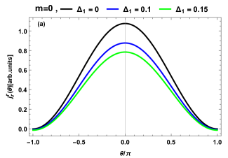
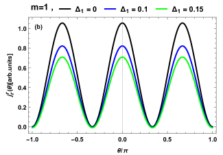
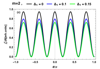
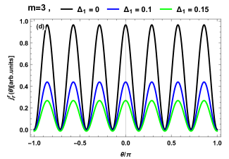
Figure 8: (color online) The radial component of the reflected density current $j_{r}^{r}$ versus the incident angle $\theta$ for $\Delta_{2}=0.2$ and $V=1$, (a): $E=0.6$ and $r_{0}=3.3$, (b): $E=0.65$ and $r_{0}=5$, (c): $E=0.69$ and $r_{0}=7.25$, (d): $E=0.35$ and $r_{0}=8.7$. Different values of the gap outside quantum dot $\Delta_{1}$ are considered.

V Conclusion

We have studied the scattering of Dirac electrons in circular graphene quantum dot through an electrostatic potential $V$ with mass-inverted terms $\Delta_{1}$ outside and $\Delta_{2}$ inside. The solutions of energy spectrum are found to be dependent on both gaps $\Delta_{1}$ and $\Delta_{2}$. Using the boundary condition at the interface, the scattering coefficients are explicitly determined. By focusing on solutions at large arguments we have used the asymptotic behavior of Hankel function to obtain analytical expressions of the radial component $j^{r}_{r}$ of current density associated to the reflected wave, the scattering efficiency $Q$ and the square modulus of the scattering coefficient $|c_{m}|^{2}$.

Our numerical analysis showed that $Q$ can be controlled by tuning the energy gap $\Delta_{1}$ outside the quantum dots. More precisely, we have observed that $Q$ decreases as long as $\Delta_{1}$ increases. Furthermore, $Q$ shows oscillatory behaviors for some chosen values of $\Delta_{1}$. Also among the obtained new results, we have observed that $\Delta_{1}$ strongly affects the behavior of $|c_{m}|^{2}$ as a function of the incident energy $E$. Indeed, $|c_{m}|^{2}$ is non-null for two energies $E=0$ and $E<\Delta_{1}$ contrary to the case of one energy gap inside the quantum dots [18]. For the radial component of the reflected current it was showed that each mode has $(2m+1)$ maximum scattering directions observable but with same amplitudes, which can be controlled under the turn on of $\Delta_{1}$.

References

- [1] K. S. Novoselov, A. R. Geim, S. V. Morozov, D. Jiang, Y. Zhang, S. V. Dubonos, I. V. Grigorieva, and A. A. Firsov, Science 306, 969 (2004).
- [2] S. Stander, B. Huard, and D. Goldhaber-Gordon, Phys. Rev. Lett. 102, 026807 (2009).
- [3] S. G. Nam, D.-K. Ki, J. W. Park, Y. Kim, J. S. Kim, and H. J. Lee, Nanotechnology 22, 415203 (2011).
- [4] A. K. Geim and K. S. Novoselov, Nature Mater. 6, 183 (2007).
- [5] M. I. Katsnelson, K. S. Novoselov, and A. K. Geim, Nat. Phys. 2, 620 (2006).
- [6] L. A. Ponomarenko, F. Schedin, M. I. Katsnelson, R. Yang, E. W. Hill, K. S. Novoselov, and A. K. Geim, Science 320, 356 (2008).
- [7] G. W. Semenoff, Phys. Rev. Lett. 53, 2449 (1984).
- [8] D. P. DiVincenzo and E. J. Mele, Phys. Rev. B 29, 1685 (1984).
- [9] Eva Cortés-del Río, Pierre Mallet, Héctor González-Herrero, José Luis Lado,Joaquín Fernández-Rossier, José María Gómez-Rodríguez, Jean-Yves Veuillen, and Iván Brihuega, Adv. Mater. 32, 2001119 (2020).
- [10] Jianhua Shen, Yihua Zhu, Xiaoling Yanga, and Chunzhong Li, Chem. Commun. 48, 3686 (2012).
- [11] Sumana Kundu and Vijayamohanan K. Pillai, Phys. Sci. Rev. 5, 0013 (2019).
- [12] N. M. R. Peres, A. H. Castro Neto, and F. Guinea, Phys. Rev. B 73, 241403 (2006).
- [13] J. M. Pereira, V. Mlinar, F. M. Peeters, and P. Vasilopoulos, Phys. Rev. B 74, 045424 (2006).
- [14] P. G. Silvestrov and K. B. Efetov, Phys. Rev. Lett. 98, 016802 (2007).
- [15] A. Matulis and F. M. Peeters, Phys. Rev. B 77, 115423 (2008).
- [16] A. Belouad, A. Jellal, and Y. Zahidi, Phys. Lett. A 380, 773 (2016)
- [17] A. Belouad, Y. Zahidi, and A. Jellal, Mater. Res. Express 3, 055005 (2016).
- [18] A. Belouad, Y. Zahidi, A. Jellal, and H. Bahlouli, EPL 123, 28002 (2018).
- [19] G. A. Steele, G. Gotz, and L. P. Kouwenhoven, Nat. Nanotech. 4, 363 (2009).
- [20] Mikhail F. Budyka, Elena F. Sheka, and Nadezhda A. Popova, Rev. Adv. Mat. Sc. 51, 35 (2017).
- [21] Lijun Liang, Xiangming Peng, Fangfang Sun, Zhe Kong, and Jia-Wei Shen, Nanoscale Adv. 3, 904 (2021).
- [22] C. Berger, Z. Song, X. Li, X. Wu, N. Brown, C. Naud, D. Mayou, T. Li, J. Hass, A. N. Marchenkov, E. H. Conrad, P. N. First, and W. A. de Heer, Science 312, 1191 (2006).
- [23] Nils M. Freitag, Larisa A. Chizhova, Peter Nemes-Incze, Colin R. Woods, Roman V. Gorbachev, Yang Cao, Andre K. Geim, Kostya S. Novoselov, Joachim Burgdörfer, Florian Libisch, and Markus Morgenstern, Nano Lett. 16, 5798 (2016).
- [24] X. Wang, G. Sun, N. Li, and P. Chen, Chem. Soc. Rev. 45, 2239 (2016).
- [25] P. V. Ratnikov, JETP Lett. (Engl. Transl.) 90, 469 (2009).
- [26] S. Rusponi, M. Papagno, P. Moras, S. Vlaic, M. Etzkorn, P. M. Sheverdyaeva, D. Pacilé, H. Brune, and C. Carbone, Phys. Rev. Lett. 105, 246803 (2011).
- [27] H. Kim, N. Leconte, B. L. Chittari, K. Watanabe, T. Taniguchi, A. H. MacDonald, J. Jung, and S. Jung, Nano Lett. 18, 7732 (2018).
- [28] Nojoon Myoung, Curr. Appl. Phys. 23, 57 (2021).