Dynamic size counting in population protocols

Abstract

The population protocol model describes a network of anonymous agents that interact asynchronously in pairs chosen at random. Each agent starts in the same initial state $s$. We introduce the dynamic size counting problem: approximately counting the number of agents in the presence of an adversary who at any time can remove any number of agents or add any number of new agents in state $s$. A valid solution requires that after each addition/removal event, resulting in population size $n$, with high probability each agent “quickly” computes the same constant-factor estimate of the value $\log_{2}n$ (how quickly is called the convergence time), which remains the output of every agent for as long as possible (the holding time). Since the adversary can remove agents, the holding time is necessarily finite: even after the adversary stops altering the population, it is impossible to stabilize to an output that never again changes.

We first show that a protocol solves the dynamic size counting problem if and only if it solves the loosely-stabilizing counting problem: that of estimating $\log n$ in a fixed-size population, but where the adversary can initialize each agent in an arbitrary state, with the same convergence time and holding time. We then show a protocol solving the loosely-stabilizing counting problem with the following guarantees: if the population size is $n$, $M$ is the largest initial estimate of $\log n$, and $s$ is the maximum integer initially stored in any field of the agents’ memory, we have expected convergence time $O(\log n+\log M)$, expected polynomial holding time, and expected memory usage of $O(\log^{2}(s)+(\log\log n)^{2})$ bits. Interpreted as a dynamic size counting protocol, when changing from population size $n_{\mathrm{prev}}$ to $n_{\mathrm{next}}$, the convergence time is $O(\log n_{\mathrm{next}}+\log\log n_{\mathrm{prev}})$.

1 Introduction

A population protocol [AADFP06] is a network of $n$ anonymous and identical agents with finite memory called the state. A scheduler repeatedly selects a pair of agents independently and uniformly at random to interact. Each agent sees the entire state of the other agent in the interaction and updates own state in response. Time complexity is measured by parallel time: the number of interactions divided by the population size $n$, capturing the natural time scale in which each agent has $\Theta(1)$ interactions per unit time. The agents collectively do a computation, e.g., population size counting: computing the value $n$. Counting is a fundamental task in distributed computing: knowing an estimate of $n$ often simplifies the design of protocols solving problems such as majority and leader election [AG15, berenbrink2018simpleLE, gkasieniec2018almost, alistarh2017time, alistarh2018space, berenbrink18majority, bennun20majority, berenbrink_2020_optimalLE, sudo2018logarithmic, MocquardAABS2015, bilke2017brief].

A protocol is defined by a transition function with a pair of states as input and as output (more generally to capture randomized protocols, a relation that can associate multiple outputs to the same input). For example, consider the simple counting protocol with transitions $L_{i},L_{j}\to L_{i+j},F_{i+j}$, with every agent starting in $L_{1}$. In population size $n$, this protocol converges to a single agent in state $L_{n}$, with all other agents in state $F_{i}$ for some $i$. The additional transitions $F_{i},F_{j}\to F_{j},F_{j}$ for $i<j$ propagate the output $n$ to all agents.

The dynamic size counting problem

In contrast to most work, which assumes the population size $n$ is fixed over time, we model an adversary that can add or remove agents arbitrarily and repeatedly during the computation. All agents start in the same state, including newly added agents. The goal is for each agent to approximately count the population size $n$, which we define to mean that all agents should eventually store the same output $k$ in their states, which with high probability is within a constant multiplicative factor of $\log n$. Once all agents have the same output $k$, they have converged. They maintain $k$ as the output for some time called the holding time (after which they might alter $k$ even if the population size has not changed). In response to a “significant” change in size from $n_{\mathrm{prev}}$ to $n_{\mathrm{next}}$, agents should re-converge to a new output $k^{\prime}$ of $\log n_{\mathrm{next}}$. (Agents are not “notified” about the change; instead they must continually monitor the population to test whether their current output is accurate.) Note that if $n_{\mathrm{prev}}$ is close to $n_{\mathrm{next}}$ (within a polynomial factor), then $k$ may remain an accurate estimate of $n_{\mathrm{next}}$, so agents may not re-converge in response to a small change.

Ideally the expected convergence time is small, and the expected holding time is large. With a fixed size population, it is common to require the output to stabilize to a value that never again changes after convergence, i.e., infinite holding time. However, this turns out to be impossible with an adversary that can remove agents (3.3). When changing from size $n_{\mathrm{prev}}$ to $n_{\mathrm{next}}$, our protocol achieves expected convergence time $O(\log n_{\mathrm{next}}+\log\log n_{\mathrm{prev}})$ and expected holding time $\Omega(n_{\mathrm{next}}^{c})$, where $c$ can be made arbitrarily large. The number of bits of memory used per agent is $O(\log^{2}(s)+(\log\log n)^{2})$, where $s$ is the maximum integer stored in the agents’ memory after the change.

While it is common to measure population protocol memory complexity by counting the number of states (which is exponentially larger than the number of bits required to represent each state), that measure is a bit awkward here. Our protocol is uniform—the same transition rules for every population size—so has an infinite number of producible states. One could count expected number of states that will be produced, but this is a bit misleading: in time $t$ each agent visits $O(t)$ states on average, so $O(t\cdot n)$ states total. Counting how many bits are required is more accurate metric of the actual memory requirements.

The loosely-stabilizing counting problem

The dynamic size counting problem has an equivalent characterization: rather than removing agents and adding them with a fixed initial state, the loosely-stabilizing adversary sets each agent to an arbitrary initial state in a fixed-size population. A protocol solves the dynamic size counting problem if and only if it solves the loosely-stabilizing counting problem, with the same convergence and holding times (Lemma 3.5). Due to this equivalence, we analyze our protocol assuming a fixed population size and adversarial initial states. In this case our convergence time $O(\log n+\log M)$ is measured as a function of the population size $n$ and the value $M$ that is the maximum $\mathtt{estimate}$ value stored in agents’ memory. From the perspective of the dynamic size counting problem, these “adversarial initial states” would correspond to the agent states after correctly estimating the previous population size, just prior to adding or removing agents.

1.1 Related work

Initialized counting with a fixed size population. In population protocols with fixed size, there is work computing exactly or approximately the population size $n$. For a full review see [doty2021survey]. Such protocols reach a stable configuration from which the output cannot change. Some of these counting protocols would still solve the counting problem in the presence of an adversary who can only add agents (see Section 3.1). However, these protocols fail in the presence of an adversary who can also remove agents, since they work only in the initialized setting and rely on reaching a stable configuration (see 3.3).

Self-stabilizing counting with a fixed size population. A population protocol is self-stabilizing if, from any initial configuration, it reaches to a correct stable configuration. Self-stabilizing size counting has been studied [AspnesBBS2016, beauquier2015space, BeauquierSS2007, IZUMI2014], but provably requires adding a “base station” agent that cannot be corrupted by the adversary. In these protocols the base station is the only agent required to learn the population size. Aspnes, Beauquier, Burman, and Sohier [AspnesBBS2016] showed a time- and space-optimal protocol that solves the exact counting problem in $O(n\log n)$ time, using $1$-bit memory for each non-base station agent.

Size regulation in a dynamically sized population. The model described by Goldwasser, Ostrovsky, Scafuro, and Sealfon [goldwasser2018population] is close to our setting. They consider the size regulation problem: approximately maintaining a target size (hard-coded into each agent) using $O(\log\log n)$ bits of memory per agent, despite an adversary that (like ours) adds or removes agents. That paper assumes a model variation in which:

• The agents can replicate or self-destruct.

• The computation happens through synchronized rounds of interactions. At each round the scheduler selects a random matching of size $k=O(n)$ agents to interact.

• The adversary’s changes to the population size are limited. The adversary can insert or delete a total of $o(n^{1/4})$ agents within each round.

The latter two model differences above crucially rule out their protocol as useful for our problem. We use the standard asynchronous scheduler, and much of the complexity of our protocol is to handle drastic population size changes (e.g., removing $n-\log n$ agents). Additionally, their protocol heavily relies on flipping coins of bias $\frac{1}{\sqrt{n}}$ that we cannot utilize since the agents don’t start with an estimate of $n$. Moreover, even when the agents compute their estimate, the population size might change.

Loosely-stabilizing leader election. Sudo, Nakamura, Yamauchi, Ooshita, Kakugawa, and Masuzawa [sudo2010looselystabilizing] introduce loose-stabilization as a relaxation for the self-stabilizing leader election problem in which the agents must know the exact population size to elect a leader. The loosely stabilizing leader election guarantees that starting from any configuration, the population will elect a leader within a short time. After that, the agents hold the leader for a long time but not forever (in contrast with self-stabilization). On the positive side, the agents no longer need to know the exact population size to solve the loosely-stabilizing leader election, but a rough upper bound suffices. Loosely-stabilizing leader election has been studied, providing a time-optimal protocol that solves the leader election problem [Sudo2021TimeoptimalLL] and a tradeoff between the holding and convergence times [izumi16, sudo2020].

Computation with dynamically changing inputs. Alistarh, Töpfer, and Uznański [alistarh2021robustComparision] consider the dynamic variant of the comparison problem. In the comparision problem, a subset of population are in the input states $X$ and $Y$ and the goal is to compute if $X>Y$ or $X<Y$. In the dynamic variant of the comparision problem, they assume an adversary who can change the counts of the input states at any time. The agents should compute the output as long as the counts remain untouched for sufficiently long time. They propose a protocol that solves the comparision problem in $O(\log n)$ time using $O(\log n)$ states per agent, assuming $|X|\geq C_{2}\cdot|Y|\geq C_{1}\log n$ for some constants $C_{1},C_{2}>1$.

Berenbrink, Biermeier, Hahn, and Kaaser [berenbrink2021selfstabilizing] consider the adaptive majority problem (generalization of the comparison problem [alistarh2021robustComparision]). At any time every agent has an opinion from $\{X,Y\}$ or undecided and their opinions might change adversarially. The goal is to have agreement in the population about the majority opinion. They introduce a non-uniform loosely-stabilizing leaderless phase clock that that uses $O(\log n)$ states to solve the adaptive majority problem. This is similar to having an adversary who can add or remove agents with different opinion. However, all agents are assumed already to have an estimate of $\log n$ that remains untouched. Thus it is not straightforward to use their protocol to solve our problem of obtaining this estimate.

2 Definitions and notation

A population protocol is a pair $\mathcal{P}=(\Lambda,\Delta)$, where $\Lambda$ is a finite set of states, and $\Delta\subseteq(\Lambda\times\Lambda)\times(\Lambda\times\Lambda)$ is the transition relation. (Often this is defined as a function $\delta:\Lambda\times\Lambda\to\Lambda\times\Lambda$, but we allow randomized transitions, where the same pair of inputs can randomly choose among multiple outputs.)

A configuration $\mathbf{c}$ of a population protocol is a multiset over $\Lambda$ of size $n$, giving the states of the $n$ agents in the population. For a state $s\in\Lambda$, we write $\mathbf{c}(s)$ to denote the count of agents in state $s$. A transition is a 4-tuple, written $\alpha:r_{1},r_{2}\to p_{1},p_{2}$, such that $((r_{1},r_{2}),(p_{1},p_{2}))\in\Delta$. If an agent in state $r_{1}$ interacts with an agent in state $r_{2}$, then they can change states to $p_{1}$ and $p_{2}$. This notation omits explicit probabilities; our main protocol’s transitions can be implemented so as to always have either one or two possible outputs for any input pair, with probability $1/2$ of each output in the latter case. For every pair of states $r_{1},r_{2}$ without an explicitly listed transition $r_{1},r_{2}\to p_{1},p_{2}$, there is an implicit null transition $r_{1},r_{2}\to r_{1},r_{2}$ in which the agents interact but do not change state. For our main protocol, we specify transitions formally with pseudocode that indicate how agents alter each independent field in their state. We say a configuration $\mathbf{d}$ is reachable from a configuration $\mathbf{c}$ if applying 0 or more transitions to $\mathbf{c}$ results in $\mathbf{d}$.

When discussing random events in a protocol of population size $n$, we say event $E$ happens with high probability if $\mathrm{Pr}\left[\neg E\right]=O(n^{-c})$, where $c$ is a constant that depends on our choice of parameters in the protocol, where $c$ can be made arbitrarily large by changing the parameters. For concreteness, we will write a particular polynomial probability such as $O(n^{-2})$, but in each case we could tune some parameter (say, increasing the time complexity by a constant factor) to increase the polynomial’s exponent.

To measure time we count the total number of interactions (including null transitions such as $a,b\to a,b$ in which the agents interact but do not change state), and divide by the number of agents $n$.

In a uniform protocol (such as the main one of this paper), the transitions are independent from the population size $n$ (see [DEMST18] for a formal definition). In other words, a single protocol computes the output correctly when applied on any population size. In contrast, in a nonuniform protocol different transitions are applied for different population sizes.

A protocol stably solves a problem if the agents eventually reach a correct configuration with probability $1$, and no subsequent interactions can move the agents to an incorrect configuration; i.e., the configuration is stable. A population protocol is self-stabilizing if from any initial configuration, the agents stably solve the problem.

3 Dynamic size counting

In a population of size $n$, define $C(n,\delta)$ to be the set of correct configurations $\mathbf{c}$ such that every agent $u$ in $\mathbf{c}$ obeys $(1-\delta)\log n<u.\mathtt{estimate}<(1+\delta)\log n$. Let $t_{h}$ be any time bound. Moreover, we define $L(n,\delta,t_{h})\subset C(n,\delta)$ the subset of correct configurations such that as the expected time for protocol $P$ starting from a configuration $\mathbf{l}\in L(n,\delta,t_{h})$ to stay in $C(n,\delta)$ is at least $t_{h}(n)$.

Definition 3.1.

Let $n_{\mathrm{prev}}$ and $n_{\mathrm{next}}$ denote the previous and next population size. A protocol $P$ solves the dynamic size counting problem if there is a $\delta>0$, called the accuracy, such that if the population size changes from $n_{\mathrm{prev}}$ to $n_{\mathrm{next}}$, the protocol reaches a configuration $\mathbf{l}$ in $L(n,\delta,t_{h})$ with high probability. The time needed to do this is called the convergence time. Moreover, $t_{h}$, the time that the population stays in $C(n_{\mathrm{next}},\delta)$, is called the holding time.

A population protocol is $\quantity(t_{c}(n),t_{h}(n))$-loosely stabilizing if starting from any initial configuration, the agents reach a correct configuration in $t_{c}(n)$ time and stay in the correct configuration for additional $t_{h}(n)$ time [sudo2010looselystabilizing, Sudo2021TimeoptimalLL]. In contrast to self-stabilizing [AAFJ08, burman2021timeoptimal], subsequent interactions can move the agents to an incorrect configuration; however, the agents recover quickly from an incorrect configuration.

Given any starting configuration $\mathbf{s}\not\in C(n,\delta)$ of size $n$, we define $f_{c}(\mathbf{s},L(n,\delta,t_{h}))$ as the expected time to reach a correct configuration in $L(n,\delta,t_{h})$.

Definition 3.2.

[sudo2010looselystabilizing, Definition 2] Let $t_{c}(n,M)$ and $t_{h}(n)$ be functions of $n$, the largest integer value $M$ in the initial configuration $\mathbf{s}$, and the set of correct configuration $C(n,\delta)$. A protocol $P$ is a $t_{c}(n,M),t_{h}\quantity(n),\delta$ loosely-stabilizing population size counting protocol if there exists a set $L(n,\delta,t_{h})$ of configurations satisfying:

For every $n$ and every initial configuration $\mathbf{s}\not\in C(n,\delta)$ of size $n$, $f_{c}(\mathbf{s},L(n,\delta,t_{h}))\leq t_{c}(n,M)$

3.1 Basic properties of the dynamic size counting problem

We first observe that the key challenge in dynamic size counting is that the adversary may remove agents. If the adversary can only add agents, the problem is straightforward to solve with optimal convergence and holding times.

Suppose the adversary in the dynamic size counting problem only adds agents. Then there is a protocol solving dynamic size counting with $O(\log n)$ convergence time (in expectation and with probability $\geq 1-O(1/n)$) and infinite holding time.

Proof 3.3.

Each agent in the initial state $s$ generates a geometric random variable. After the last time that the adversary adds agents, resulting in $n$ total agents, exactly $n$ geometric random variables will have been generated. Agents propagate the maximum by epidemic using transition $a,b\to\max(a,b),\max(a,b)$, taking $3\ln n$ time to reach all agents with probability

$\geq 1-\frac{1}{n^{2}}$ [burman2021timeoptimal, Corollary 2.8]. The maximum of $n$ i.i.d. geometric random variables is in the range $[\log n-\log\ln n,2\log n]$ with probability $\geq 1-\frac{1}{n}$ [doty2018efficient, Lemma D.7].

In contrast, if the adversary can remove agents, then even if it is guaranteed to do this exactly once, no protocol can be stabilizing, i.e., have infinite holding time. Suppose the adversary in the dynamic size counting problem will remove agents exactly once. Then any protocol solving the problem has finite holding time.

Proof 3.4.

Suppose otherwise. Let the initial population size be $n$ and the later size be $n^{\prime}<n$. The protocol must handle the case where the adversary never removes agents, since in population size $n$ this is equivalent to an adversary who starts with $n+1$ agents and immediately removes one of them. Thus if the adversary waits sufficiently long before the removal, then all agents stabilize to output $k=\Theta(\log n)$. In other words, no sequence of transitions can alter the value, including transitions occurring only among any subpopulation of size $n^{\prime}$. So after the adversary removes $n-n^{\prime}$ agents, the remaining $n^{\prime}$ agents are unable to alter the output $k$, a contradiction if $n^{\prime}$ is sufficiently small compared to $n$.

Lemma 3.5 shows that the dynamic size counting problem is equivalent to the loosely-stabilizing counting problem. Due to this equivalence, our correctness proofs will use the loosely-stabilizing characterization.

To prove Lemma 3.5, we require the following result, proven in [doty2018efficient, Lemma 4.2]. It states that for any finite set $\Lambda_{f}$ of states producible in a protocol from a uniform initial state, for any sufficiently large initial population size $n$, WHP many copies of each state in $\Lambda_{f}$ appear.

Lemma 3.5 ([doty2018efficient]).

Let $P$ be a population protocol, and let $\Lambda_{f}$ be a finite set of states, each producible in $P$ from sufficiently many agents in state $s$. Then there are constants $\epsilon,\delta,n_{0}>0$ such that, for all $n\geq n_{0}$, starting from $n$ agents in state $s$, if $\mathbf{d}$ is the configuration reached at time $1$, then $\mathrm{Pr}\left[(\forall q\in\Lambda_{f})\ \mathbf{d}(q)\geq\delta n\right]\geq 1-2^{-\epsilon n}.$

Recall that we define $M$ as the largest integer value the agents stored in the starting configuration $\mathbf{s}$.

inline]The following lemma is proven in the full version of this paper. [add citation?] A protocol solves the dynamic size counting problem with convergence time $t_{c}(n,M)$ and holding time $t_{h}(n)$ if and only if it solves the loosely-stabilizing counting problem with convergence time $t_{c}(n,M)$ and holding time $t_{h}(n)$.

Any states present in an adversarially prepared configuration $\mathbf{c}$ will be produced in large quantities from any sufficiently large initial configuration of all initialized states $s$ [doty2018efficient, Lemma 4.2]. The dynamic size adversary can then remove agents to result in $\mathbf{c}$, which the protocol must handle, showing it can handle an arbitrary initial configuration.

Proof 3.6.

The easy direction is that if the protocol $P$ solves the loosely-stabilizing counting problem, then it solves the dynamic size counting problem. Starting from any possible configuration $\mathbf{s}$ of size $n$, with largest integer $M$, $P$ converges in time $t_{c}(n,M)$ with holding time $t_{h}(n)$. The configuration immediately after the dynamic size adversary adds or removes agents is simply one of the configurations that $P$ is able to handle.

To see the reverse direction, suppose $P$ solves the dynamic size counting problem; we argue that $P$ also solves the loosely-stabilizing counting problem. Let $\mathbf{c}$ be any configuration of $P$. The dynamic size adversary can do the following to reach configuration $\mathbf{c}$. Let $\Lambda_{f}=\{q\mid\mathbf{c}(q)>0\}$ be the set of states in $\mathbf{c}.$ Apply Lemma 3.5 with this choice of $\Lambda_{f}$. Choose $n$ sufficiently large that $\delta n\geq\max_{q\in\Lambda_{f}}\mathbf{c}(q)$. Then Lemma 3.5 says that starting from $n$ agents in state $s$, with probability at least $1-2^{-\epsilon n}$, in the configuration $\mathbf{d}$ at time 1, for all $q\in\Lambda_{f}$, $\mathbf{d}(q)\geq\delta n\geq\mathbf{c}(q)$. Thus $\mathbf{d}\geq\mathbf{c}$. Now the adversary removes agents from $\mathbf{d}$ to result in $\mathbf{c}$. Let $n^{\prime}=\|\mathbf{c}\|$. The protocol converges from $\mathbf{c}$ with largest integer $M^{\prime}$ in time $t_{c}(n,M^{\prime})$, with holding time $t_{h}(n)$. But since $\mathbf{c}$ is an arbitrary configuration of the protocol, this implies that $P$ solves the loosely-stabilizing counting problem.

3.2 High-level overview of dynamic size counting protocol

In this section we briefly describe our protocol solving the dynamic size counting, which is defined formally in Section 3.3. By Lemma 3.5 it suffices to design a protocol solving the loosely-stabilizing counting problem for a fixed population size $n$. Our protocol uses the “detection” protocol of [alistarh17detection]. Consider a subset of states designated as a “source”. A detection protocol alerts all agents whether a source state is present in the population.

In Protocol 1, the population maintains several dynamic groups, with the agent’s group stored as a positive integer field $\mathtt{group}$. The $\mathtt{group}$ values are not fixed: each agent changes its $\mathtt{group}$ field on every interaction, with equal probability either incrementing $\mathtt{group}$ or setting it to 1. We show that, no matter the initial group values, after $O(\log n)$ time the group values will be in the range $[1,8\log n]$ WHP. The distribution of $\mathtt{group}$ values is very close to that of $n$ i.i.d. geometric random variables, in the sense that each agent’s $\mathtt{group}$ value is independent of every other, with expected $n/2^{i}$ agents having $\mathtt{group}=i$ if each agent has had at least $i$ interactions.

The agents store an array of “signal” integers in their $\mathtt{signals}$ field, as a way to track the existing $\mathtt{group}$ values in the population. Each agent in the $i$’th group is responsible to boost the signal associated with $i$. The goal is to have $\mathtt{signals}[i]>0$ for all agents if and only if some agent has $\mathtt{group}=i$.

The detection protocol of [alistarh17detection], explained below, provides a technique for agents to know which groups are still present. Once a signal for group $k$ fades out, the agents speculate that there is no agent with $\mathtt{group}=k$. Depending on the current value stored as $\mathtt{estimate}$ in agents’ memory and the value $k$, this might cause re-calculating the population size. The agents are constantly checking for the changes in the $\mathtt{signals}$. They re-compute $\mathtt{estimate}$ once there is a large gap between $\mathtt{estimate}$ and the first $\mathtt{group}$ $i$ with $\mathtt{signals}[i]=0$. We call $i$ the first missing value (stored in the field $\mathtt{FMV}$).

The $\mathtt{signals}$ array is updated as follows. An agent with $\mathtt{group}=k$ sets $\mathtt{signals}[k]$ to its maximum possible value ($3k+1$); we call this boosting. Other groups $k$ are updated between two agents $u,v$ with $u.\mathtt{signals}[k]=a$ and $v.\mathtt{signals}[k]=b$ via propagation transitions that set both agent’s $\mathtt{signals}[k]$ to $\max(a-1,b-1,0)$. The paper [alistarh17detection] used a nonuniform protocol where each agent already has an estimate of $\log n$. They prove that if the state being detected (in our case, a state with $\mathtt{group}=k$) is absent and the current maximum signal is $c$, then all agents will have signal 0 within $\Theta(c)$ time. However, if the state being detected is present, then the boosting transitions (occurring every $O(1)$ units of parallel time on average in the worst case that its count is only 1) will keep the signal positive in all agents with high probability. For this to hold, it is critical that the maximum value set during boosting is $\Omega(\log n)$; the nonuniform protocol of [alistarh17detection] uses its estimate of $\log n$ for this purpose.

Crucially, our protocol associates smaller maximum signal values to smaller group values (so many are much smaller than $\log n$), to ensure that a signal does not take abnormally long to get to 0 when its associated group value is missing. Otherwise, if we set each signal value to $\Omega(\log n)$ (based on the agent’s current estimate $\mathtt{estimate}$ of $\log n$) during boosting, then it would take time proportional to $\mathtt{estimate}$ (which could be much larger than the actual value of $\log n$) to detect the absence of a $\mathtt{group}$ value. Thus is it critical that we provide a novel analysis of the detection protocol, showing that the signals for smaller group values $k\ll\log n$ remain present with high probability. This requires arguing that the boosting reactions for such smaller values are happening with sufficiently higher frequency, due to the higher count of agents with $\mathtt{group}=k$, to compensate for the smaller boosting signal values they use.

3.3 Formal description of loosely-stabilizing counting protocol

The ${\mathrm{DynamicCounting}}$ protocol (Protocol 1) divides agents among $\Theta(\log n)$ groups via the $\mathrm{UpdateGroup}$ subprotocol. The agents update their $\mathtt{group}$ from $i$ to $i+1$ with probability $1/2$ or reset to group $1$ with probability $1/2$. The number of agents at each group and the total number of groups are both random variables that are dynamically changing through time. We show that the total number of groups remains close to $\log n$ at all times with high probability.

The agents start with arbitrary (or even adversarial) $\mathtt{group}$ values but we show that WHP the set of $\mathtt{group}$ values will converge to $[1,8\log n]$ within $O(\log n)$ time (Corollary 5.6). Additionally, each agent stores an array of $O(\log n)$ signal values in their $\mathtt{signals}$ field. It is crucial for agents to maintain positive values in the $\mathtt{signals}[i]$ if some agent has $\mathtt{group}=i$. They use the first $\mathtt{group}$ $i$ with $\mathtt{signals}[i]=0$ (stored in $\mathtt{FMV}$). The agents use $\mathtt{FMV}$ as an approximation of $\log n$ and constantly compare it with their $\mathtt{estimate}$ value.

Depending on the $\mathtt{estimate}$ value stored in agents’ memory, the agents maintain 3 main phases of computation:

$\mathsf{NormalPhase}$:

An agent stays in the $\mathsf{NormalPhase}$ as long as there is a small gap between $\mathtt{estimate}$ and $\mathtt{FMV}$: $0.25\cdot\mathtt{estimate}\leq\mathtt{FMV}\leq 2.5\mathtt{estimate}$.

$\mathsf{WaitingPhase}$:

An agent switches from $\mathsf{NormalPhase}$ to $\mathsf{WaitingPhase}$ if it sees a large gap between the $\mathtt{FMV}$ and $\mathtt{estimate}$: $\mathtt{FMV}\not\in\{0.25\cdot\mathtt{estimate},\ldots,2.5\cdot\mathtt{estimate}\}$. The purpose of $\mathsf{WaitingPhase}$ is to give enough time to the other agents so that by the end of the $\mathsf{WaitingPhase}$ for one agent, with high probability every other agent has also noticed the large gap between the $\mathtt{FMV}$ and $\mathtt{estimate}$ and entered $\mathsf{WaitingPhase}$.

$\mathsf{UpdatingPhase}$:

During the $\mathsf{UpdatingPhase}$, every agent use a new geometric random variable and propagates the maximum by epidemic. We set $\mathsf{WaitingPhase}$ long enough so that with high probability when the first agent switches to the $\mathsf{UpdatingPhase}$, the rest of the population are all in $\mathsf{WaitingPhase}$. By the end of $\mathsf{UpdatingPhase}$, every agent switches back to $\mathsf{NormalPhase}$.

Below we explain each subprotocol in more detail.

Protocol 1 ${\mathrm{DynamicCounting}}(\mathrm{u},\mathrm{v})$

for $\mathrm{agent}\in\{\mathrm{u},\mathrm{v}\}$ do

     $\mathrm{UpdateGroup}(\mathrm{agent})$

$\mathrm{SignalPropagation}(\mathrm{u},\mathrm{v})$

for $\mathrm{agent}\in\{\mathrm{u},\mathrm{v}\}$ do

     $\mathrm{UpdateMV}(\mathrm{agent})$

     $\mathrm{SizeChecker}(\mathrm{agent})$

     if $\mathrm{agent}.\tt{phase}\neq\mathsf{NormalPhase}$ then

         $\mathrm{TimerRoutine}(\mathrm{agent})$      

$\mathrm{PropagateMaxEst}(\mathrm{u},\mathrm{v})$

for $\mathrm{agent}\in\{\mathrm{u},\mathrm{v}\}$ do

     if $\mathrm{agent}.\tt{phase}=\mathsf{NormalPhase}$ then

         $\mathrm{agent}.\mathtt{estimate}\leftarrow\mathrm{agent}.\mathtt{GRV}$      

In every interaction, both sender and receiver update their group according to the rules of the $\mathrm{UpdateGroup}$ subprotocol. If we look at the distribution of the $\mathtt{group}$ values after $O(\log n)$ time, there are about $n/2$ agents in group $1$, $n/4$ agents in group $2$ and $n/2^{i}$ agents in group $i$ (see Figure 4). Note that the number of agents in each group decreases exponentially, but we ensure that agents with larger $\mathtt{group}$ values use stronger signals to propagate, since there is less support for those groups.

Protocol 2 $\mathrm{UpdateGroup}(\mathrm{agent}\ \mathrm{u})$

$\mathrm{u}.\mathtt{group}\leftarrow\begin{cases}\mathrm{u}.\mathtt{group}+1&\text{with probability }1/2\\ 1&\text{with probability }1/2\end{cases}$

To notify all agents about the set of all $\mathtt{group}$ values that are generated among the population, we use the detection protocol of [alistarh17detection] that is also used as a synchronization scheme in [berenbrink2021selfstabilizing]. The agents store an integer for each $\mathtt{group}$ value that is generated by the population. The $\mathtt{signals}$ is an array of length $\Theta(\log n)$ such that a positive value in index $i$ represents some agents in the population have generated $\mathtt{group}=i$. Note that, as an agent updates its $\mathtt{group}$, it boosts multiple signals based on its $\mathtt{group}$ value, e.g., an agent with $\mathtt{group}=i$ helped boosting all the indices $1,2,3,\ldots,i$ of $\mathtt{signals}$ in its last $i$ interactions. We use the $\mathrm{SignalPropagation}$ protocol to keep the signal of group $i$ positive as long as some agents have generated $\mathtt{group}=i$.

Algorithm 3 $\mathrm{SignalPropagation}(\mathrm{agent}\ \mathrm{u},\mathrm{agent}\ \mathrm{v})$

$\triangleright$ Boosting:

$\mathrm{u}.\mathtt{signals}[\mathrm{u}.\mathtt{group}]\leftarrow(3\cdot\mathrm{u}.\mathtt{group})+1$

$\mathrm{v}.\mathtt{signals}[\mathrm{v}.\mathtt{group}]\leftarrow(3\cdot\mathrm{v}.\mathtt{group})+1$

$\triangleright$ Propagate signal:

for $i\in\{1,2,\ldots,\texttt{Max}(|\mathrm{u}.\mathtt{signals}|,|\mathrm{v}.\mathtt{signals}|\}$ do

     $m\leftarrow\texttt{Max($\mathrm{u}.\mathtt{signals}[i],\mathrm{v}.\mathtt{signals}[i]$)}$

     $\mathrm{u}.\mathtt{signals}[i],\mathrm{v}.\mathtt{signals}[i]\leftarrow\texttt{Max}(0,m-1)$

Regardless of the initial configuration, the distribution of $\mathtt{group}$ values changes immediately (in $O(\log n)$ time) but it might take more time for the $\mathtt{signals}$ to get updated. It takes $O(i)$ time for $\mathtt{signals}[i]$ to hit zero. The larger the index $i$, $\mathtt{signals}[i]$ leaves the population slower. Hence, the agents look at the first missing signal that they observe among the array of all signals.

Algorithm 4 $\mathrm{UpdateMV}(\mathrm{agent}\ \mathrm{u})$

$\triangleright$ Finds the first appearance of a zero in $u.\mathtt{signals}$ beyond index $\lceil\texttt{log}(\mathrm{u}.\mathtt{estimate})\rceil$

$s\leftarrow\lceil\texttt{log}(\mathrm{u}.\mathtt{estimate})\rceil$

$\mathrm{u}.\mathtt{FMV}\leftarrow\min\{i\in[s,|\mathrm{u}.\mathtt{signals}|]\mid\mathrm{u}.\mathtt{signals}[i]=0\}$

Once there is a large gap between the first missing $\mathtt{group}$ ($\mathtt{FMV}$) and the agents’ estimation of $\log n$ ($\mathtt{estimate}$), each agent individually moves to a waiting phase and waits for other agents to catch the same gap between their $\mathtt{estimate}$ and $\mathtt{FMV}$. Note that, we time this phase as a function of $\mathtt{FMV}$ and not the $\mathtt{estimate}$ since the $\mathtt{estimate}$ is not valid anymore and might be much smaller or larger that the true value of $\log n$.

Algorithm 5 $\mathrm{SizeChecker}(\mathrm{u})$

if $\mathrm{u}.\tt{phase}=\mathsf{NormalPhase}$ then

     if $\mathrm{u}.\mathtt{FMV}\not\in\{0.25\cdot\mathrm{u}.\mathtt{estimate},\ldots,2.5\cdot\mathrm{u}.\mathtt{estimate}\}$ then

         $\mathrm{u}.\tt{phase}\leftarrow\mathsf{WaitingPhase}$

         $\mathrm{u}.\mathtt{timer}\leftarrow 1$ $\triangleright$ Waiting for the other agents to detect the size change      

Eventually all agents will notice the large discrepancy between $\mathtt{FMV}$ and $\mathtt{estimate}$, and move to the $\mathsf{WaitingPhase}$. The $\mathsf{WaitingPhase}$ is followed by the $\mathsf{UpdatingPhase}$ (explained in the $\mathrm{TimerRoutine}$). In the $\mathsf{UpdatingPhase}$ all agents generate one geometric random variable (stored in $\mathtt{GRV}$) and start propagating the maximum value. For the purpose of representation, we assume the agents generate a geometric random variable in one line (line 4 in 6).

Once the $\mathsf{UpdatingPhase}$ is finished all agents will update their $\mathtt{estimate}$ to the maximum geometric random variable they have seen and switch to the $\mathsf{NormalPhase}$ again.

Algorithm 6 $\mathrm{TimerRoutine}(\mathrm{u})$

$\mathrm{u}.\mathtt{timer}\leftarrow\mathrm{u}.\mathtt{timer}+1$

if $\mathrm{u}.\mathtt{timer}>12\cdot\mathrm{u}.\mathtt{FMV}$ then

     if $\mathrm{u}.\tt{phase}=\mathsf{WaitingPhase}$ then

         $\mathrm{u}.\mathtt{GRV}\leftarrow$a new geometric random variable

         $\mathrm{u}.\tt{phase}\leftarrow\mathsf{UpdatingPhase}$

         $\mathrm{u}.\mathtt{timer}\leftarrow 1$      

     if $\mathrm{u}.\tt{phase}=\mathsf{UpdatingPhase}$ then

         $\mathrm{u}.\mathtt{estimate}\leftarrow\mathrm{u}.\mathtt{GRV}$

         $\mathrm{u}.\tt{phase}\leftarrow\mathsf{NormalPhase}$

         $\mathrm{u}.\mathtt{timer}\leftarrow 0$      

Recall that the agents remain in the $\mathsf{NormalPhase}$ as long as their $\mathtt{FMV}$ and $\mathtt{estimate}$ are fairly close. They continue changing their $\mathtt{group}$ values and send group signals as described earlier.

Algorithm 7 $\mathrm{PropagateMaxEst}(\mathrm{agent}\ \mathrm{u},\mathrm{agent}\ \mathrm{v})$

if $\mathrm{u}.\tt{phase}=\mathrm{v}.\tt{phase}\And\mathrm{u}.\tt{phase}\neq\mathsf{WaitingPhase}$ then

     $\mathrm{u}.\mathtt{GRV},\mathrm{v}.\mathtt{GRV}\leftarrow\mathrm{max}(\mathrm{u}.\mathtt{GRV},\mathrm{v}.\mathtt{GRV})$

Intuitively, for each $\mathtt{group}$ value, about $n/2^{i}$ agents will hold $\mathtt{group}=i$, and try to boost $\mathtt{signals}[i]$ by setting it to the max $=\Theta(i)$. As the value of $i$ grows, the number of agents with $\mathtt{group}=i$ decreases, but their signals get stronger since the agents enhance a $\mathtt{group}$ signal $i$ proportional to $i$. In a normal run of the protocol, the agents expect to have positive values in $\mathtt{signals}[i]$ for $\mathtt{group}$ values between $[\log\ln n,\log n]$.

4 Simulation results

In this section, we present our simulation results for Protocol 1. We present two separate simulation results, one starting with a uniformly random initial configuration (Figure 1) in which each agent starts with a random number (bounded by $60$) in each of their $\mathtt{group}$ and $\mathtt{estimate}$ fields. Additionally, we set a random integer of $\Theta(i)$ in each index of their $\mathtt{signals}$. In Figure 1, we depict the $\mathtt{group}$ and $\mathtt{signals}$ fields of the agents in a population size $n=10^{6}$. We can observe the changes in the $\mathtt{group}$ and $\mathtt{signals}$ within multiple snapshots from the population.

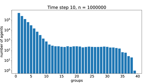
(a) The distribution of $\mathtt{group}$ values at $t=10$. Observe that for all $\mathtt{group}$ values less than $10$, the distribution is close to the stationary distribution in which about $\frac{n}{2^{i}}$ agents have $\mathtt{group}=i$. However, it is too soon for all “unwanted” group values to disappear.

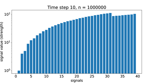
(b) Snapshot of the population at time $10$: the distribution of $\mathtt{signals}$ values. The data shows $min(u.\mathtt{signals}[i])$ for every index $i$ and agent $u\in\mathcal{A}$. Note that, for every index $i$, $\mathtt{signals}[i]$ now has a positive value.

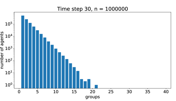
(c) Snapshot of the population at time $30$: the distribution of $\mathtt{group}$ values reached the stationary distribution.

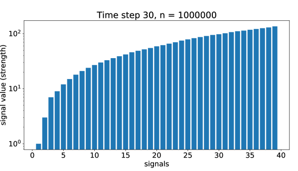
(d) Snapshot of the population at time $30$: even though there is no agent with $\mathtt{group}>25$, the $\mathtt{signals}$ for all $\mathtt{group}$s are still positive.

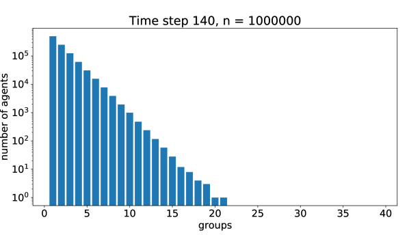
(e) Snapshot of the population at time $140$: the distribution of $\mathtt{group}$ values reached the stationary distribution and stays the same for polynomial time.

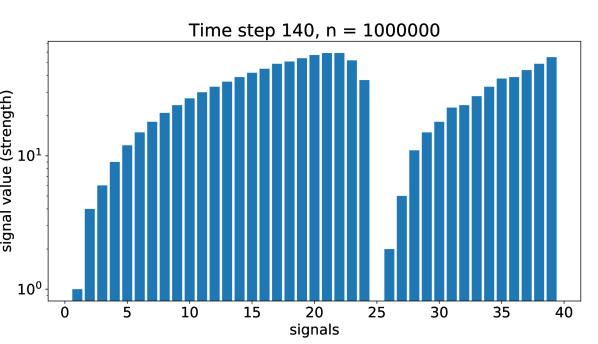
(f) Snapshot of the population at time $140$: the emergence of the $\mathtt{FMV}=25$ which is in $O(\log n)$ for the entire population. Note that in our protocol the agents don’t wait for all values of $25$ and greater to disappear. Having $\mathtt{signals}[i]=0$ for one index $i$ suffices to re-calculate the $\mathtt{estimate}$.

Figure 1: inline]DD: The text in the figures should be made larger. Simulation results for population size =$10^{6}$. Initializing each agent with a random $1\leq\mathtt{group}<30$, and for every $1\leq i\leq 60$, $0\leq\mathtt{signals}[i]\leq 3\cdot i+1$ in $\mathsf{NormalPhase},\mathsf{WaitingPhase},$ or $\mathsf{UpdatingPhase}$ with probability $1/3$. Plots of the $\mathtt{signals}$ for a randomly initialized population. The x-axis shows all the indices in the $\mathtt{signals}$ of the agents (bounded by $40$ in the simulation). On the y-axis, and every index $i$, we take the minimum pairwise value of $u.\mathtt{signals}[i]$ for all $u\in\mathcal{A}$.

(a) The distribution of $\mathtt{estimate}$ during the course of a computation. First, the agents agree on $\mathtt{estimate}=20$ and keep their estimate throughout the computation. This simulation shows how the agents update their $\mathtt{estimate}$ once we removed $O(n)$ agents from the original population.

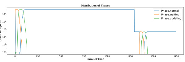
(b) The distribution of $\tt{phase}$ values. This simulation shows how the agents update their $\mathtt{estimate}$ by going through $\mathsf{WaitingPhase}$ and $\mathsf{UpdatingPhase}$ consecutively.

Figure 2: Simulation results for population size $n=400000\approx 2^{18}$. Initializing each agent with $\mathtt{group}=1$, and an empty $\mathtt{signals}$ in $\mathsf{NormalPhase}$. First, the agents calculate the $\mathtt{estimate}$ for $n=2^{18}$, then at time $\leavevmode\nobreak\ 1350$ we remove all but $500$ agents randomly which results in updating the agents’ $\mathtt{estimate}$ from $20$ to $10$.

In our second simulation, we initialized the population with default values (starting in the initialized setting), however, after the population converges to an $\mathtt{estimate}$ of $O(\log n)$ we remove agents uniformly at random to simulate an adversarial initialized population. The result of this simulation is shown in Figure 2.

5 Analysis of ${\mathrm{DynamicCounting}}$

5.1 Useful time bounds

Let $n$ and $\mathcal{A}$ be the population size and the set of agents in the population respectively. Let $I(t,u)$ represent the number of interactions involving agent $u$ by the time $t$. Also, let $G_{u,t}$ represent the $\mathtt{group}$ value for agent $u$ at time $t$ calculated via the rules defined in Protocol 2.

For any $d\geq 3$ and $2d/3\geq c\geq 1$ during $dn\ln n$ interaction, all agents have at least $2(d-\sqrt{dc})\ln n$ and at most $2(d+\sqrt{3dc/2})\ln n$ interactions with arbitrary large probability $1-n^{1-c}$.

Let us consider a fixed agent $u$. Recall that we defined $I(t,u)$ to be the number of interactions involving agent $u$ in $t$ time. Note that $I(t,u)$ has a binomial distribution with parameters $\mathsf{B}(dn\ln n,2/n)$ with $\mu=2d\ln n$ for $t=d\ln n$. We can get a tight bound on the expected value using a straightforward Chernoff bound:

For the lower bound:

$$\mathrm{Pr}\left[I(t,u)\leq(1-\delta)\mu\right] \leq e^{-\delta^{2}\mu/2}$$ (1)

$$\mathrm{Pr}\left[I(t,u)\leq(1-\delta)2d\ln n\right] \leq e^{-\delta^{2}(2d\ln n)/2}$$ (2)

$$\mathrm{Pr}\left[I(t,u)\leq(1-\delta)2d\ln n\right] \leq n^{-\delta^{2}d}$$ (3)

$$\mathrm{Pr}\left[I(t,u)\leq 2(d-\sqrt{dc})\ln n\right] \leq n^{-c} \delta=\sqrt{c/d}\leq 1$$ setting (4)

With a union bound we can show that $\mathrm{Pr}\left[I(t,u)\leq 2(d-\sqrt{dc})\ln n\right]\leq n^{1-c}$ for all agents.

and for the upper bound:

$$\mathrm{Pr}\left[I\quantity(t,u)\geq\quantity(1+\delta)\mu\right] \leq e^{-\delta^{2}\mu/(2+\delta)}$$ (5)

$$\mathrm{Pr}\left[I\quantity(t,u)\geq\quantity(1+\delta)2d\ln n\right] \leq e^{-\delta^{2}\quantity(2d\ln n)/3} 0\leq\delta\leq 1$$ for (6)

$$\mathrm{Pr}\left[I\quantity(t,u)\geq\quantity(1+\delta)2d\ln n\right] \leq n^{-2\delta^{2}d/3}$$ (7)

$$\mathrm{Pr}\left[I\quantity(t,u)\geq 2\quantity(d+\sqrt{3dc/2})\ln n\right] \leq n^{-c} \delta=\sqrt{3c/2d}\leq 1$$ setting (8)

A union bound shows that $\mathrm{Pr}\left[I\quantity(t,u)\geq 2\quantity(d+\sqrt{3dc/2})\ln n\right]\leq n^{1-c}$ for all agents.

Corollary 5.1.

For any $d\geq 3$, during $dn\ln n$ interaction, all agents have at least $0.2d\ln n$ and at most $4d\ln n$ interactions with probability $1-n^{1-2d/3}$.

Proof 5.2.

Setting $c=2d/3$ in Section 5.1 results in the above bounds.

5.2 Bound on the group values

Recall that the agents calculate a dynamic $\mathtt{group}$ value by following the rules of Protocol 2. As described in this protocol, the agents move through different $\mathtt{group}$ values according to the Markov chain shown in Figure 3.

Figure 3: The infinite chain of $\mathtt{group}$ values.

In this part, we analyze the distribution of $\mathtt{group}$ values. Note that at the very beginning of the protocol, the $\mathtt{group}$ values are rather chaotic since the agents might start holding any arbitrary $\mathtt{group}$ values that are much larger than $\log n$. However, after all agents reset back to $\mathtt{group}=1$, we can show for each $\mathtt{group}=k$, $\mathrm{Pr}\left[\mathtt{group}=k\right]\approx\frac{1}{2^{k}}$.

In the rest of this section we assume the initialized setting for simplicity. Later on we show how we can generalize our results to any arbitrary initial configuration. Recall that $G_{u,t}$ stands for the $\mathtt{group}$ value of agent $u$ at time $t$ and $I(t,u)$ shows the number of interactions involving this agent by the time $t$. Note that with this definition, $G_{u,t}$ is equal to $k$ (for $k<I(t,u)$) if and only if agent $u$ generates the sequence of $[HTTT\ldots T]$ (H followed by $k-1$ Ts) during its last $k$ interactions. Thus, we have:

$$\forall k\in\mathbb{N},\quad 1\leq k<I(t,u):\mathrm{Pr}\left[G_{u,t}=k\right]=\frac{1}{2^{k}}$$ (9)

With this definition $G_{u,t}$ is undefined for any agents that has not generated $H$ yet. In other words, the values $G_{u,t}$ are “close to geometric” in the sense that they are independent and have probability equal to a geometric random variable on all values $k<I(t,u)$.

For agents $u_{1},u_{2},\ldots,u_{n}$, and the values $k_{i}<I(t,u_{i})$, for $1\leq i\leq n$:

$$\mathrm{Pr}\left[G_{u_{1},t}=k_{1},G_{u_{2},t}=k_{2},\ldots,G_{u_{n},t}=k_{n}\right]=\prod_{i=1}^{n}\mathrm{Pr}\left[G_{u_{i},t}=k_{i}\right]$$

Next we bound the maximum $\mathtt{group}$ value that has been generated by any agent. Let $M_{t}=\max_{u\in\mathcal{A}}G_{u,t}$ be the maximum value of $G_{u,t}$ across the population at time $t$.

Let $c\geq 2$ and let $t$ be a time such that all agents have at least $c\log n$ interactions. In a population of size $n$, $\frac{1}{d}\log n\leq M_{t}$ with probability at least $1-\mathrm{exp}\left(-n^{1-1/d}\right)$ and $M_{t}<c\log n$ with probability at least $1-n^{1-c}$.

Recall that $G_{u,t}$ is the $\mathtt{group}$ value of agent $u$, $I(t,u)$ is the number of interactions that this agent had by the time $t$, and $M_{t}$ is the maximum value of $G_{u,t}$ for all $u\in\mathcal{A}$ at time $t$. Since all agents have had at least $c\log n$ interactions, for all values of $k<c\log n$, $\mathrm{Pr}\left[G_{u,t}=k\right]=\frac{1}{2^{k}}$. To have $M_{t}\geq c\log n$, at least one agent must have generated a $\mathtt{group}$ value greater than or equal to $c\log n$:

$$\mathrm{Pr}\left[M_{t}\geq c\log n\right] =\mathrm{Pr}\left[\quantity(\exists u\in\mathcal{A})G_{u,t}\geq c\log n\right]$$

$$\leq n\cdot\quantity(\frac{1}{2})^{c\log n}\quad\text{by the union bound}$$

$$=n^{1-c}$$

For the other direction, to have $M_{t}>\frac{1}{d}\log n$, at least one agent must have generated $\mathtt{group}>\frac{1}{d}\log n$. By Section 5.2:

$$\mathrm{Pr}\left[M_{t}<\frac{1}{d}\log n\right] =\mathrm{Pr}\left[\quantity(\forall u\in\mathcal{A})G_{u,t}<\frac{1}{d}\log n\right]$$

$$=\quantity(1-\frac{1}{2^{1/d\log n}})^{n}$$

$$=\quantity(1-\frac{1}{n^{1/d}})^{n}$$

$$=\quantity(1-\frac{n^{1-1/d}}{n})^{n}$$

$$\leq\mathrm{exp}\left(-n^{1-1/d}\right).$$

Additional to bounds on the maximum $\mathtt{group}$ value, we need to calculate the bounds for the first missing $\mathtt{group}$. Note that the maximum $\mathtt{group}$ value has a large variance, however, we can prove a tight bound for the first missing $\mathtt{group}$ since to have $\mathtt{FMV}=k$, for all values $i$ that are less than $k$, $\exists u\in\mathcal{A}$ such that $u.\mathtt{group}=i$ .

5.3 Bounds on the first missing group

In this part, we analyze the bounds for the first $\mathtt{group}$ value that has no support, i.e., the value $\min\{k\in\mathbb{N}^{+}\mid(\forall u\in\mathcal{A})\ u.\mathtt{group}\neq k\}$. Considering $n$ i.i.d. geometric random variables, the first missing value to be the smallest integer not appearing among the random variables. The first missing value has been studied in the literature [louchard2005number, prodinger2021philippe, louchard2004moments] as the “the first empty urn” (see also “probabilistic counting” [flajolet1985probabilistic]) but for simplicity we use a loose bound for our analysis.

Let $\delta>0$, $0<\epsilon<1$ and let $t$ be a time such that all agents have at least $(1+\delta)\log n$ interactions. Define $\mathtt{FMV}_{t}=\min\{k\in\mathbb{N}\mid(\forall u\in\mathcal{A})\ u.\mathtt{group}\neq k\}$ at time $t$. Then, $\mathtt{FMV}_{t}>(1-\epsilon)\log n$ with probability at least $(1-\epsilon)\log(n)\cdot\mathrm{exp}\left(-n^{\epsilon}\right)$ and $\mathtt{FMV}_{t}\leq(1+\delta)\log n$ with probability at least $1-\quantity(\frac{1}{n^{\delta/2}})^{(2+\delta)\log n}$. Recall that we use $I(u,t)$ to represent the number of interactions agent $u$ had by time $t$. Also, we use $G_{u,t}$ to show $u.\mathtt{group}$ at time $t$.

For any $\mathtt{group}$ value $k$ that $k<I(u,t)$, we have $\mathrm{Pr}\left[G_{u,t}=k\right]=\frac{1}{2^{k}}$ (Equation 9). We say group $i$ is missing if $i\neq G_{u,t}$ for all $u\in\mathcal{A}$. Since the $G_{u,t}$’s are independent (across different agents $u$ for a fixed $t$), For any $1\leq i\leq c\log n$, the probability that $i$ is missing is $\quantity(1-\frac{1}{2^{i}})^{n}\approx\mathrm{exp}\left(-\frac{n}{2^{i}}\right)$. We take a union bound on all $1\leq i\leq\epsilon\log n$:

$$\mathrm{Pr}\left[\mathtt{FMV}_{t}\leq(1-\epsilon)\log n\right] \leq\sum_{i=1}^{(1-\epsilon)\log n}\quantity(1-\frac{1}{2^{i}})^{n}$$

$$\leq\sum_{i=1}^{(1-\epsilon)\log n}\mathrm{exp}\left(-\frac{n}{2^{i}}\right)$$

$$\leq(1-\epsilon)\log(n)\cdot\mathrm{exp}\left(-\frac{n}{2^{(1-\epsilon)\log n}}\right) \quantity(1+\frac{x}{n})^{n}\leq\mathrm{exp}\left(x\right)$$ since

$$=(1-\epsilon)\log(n)\cdot\mathrm{exp}\left(-n^{\epsilon}\right)$$

For the upper bound, inline]Add something about negative dependence

$$\mathrm{Pr}\left[\mathtt{FMV}_{t}>U\right] \leq\prod_{i=1}^{U}\mathrm{Pr}\left[\quantity(\exists u\in\mathcal{A})G_{u,t}=i\right]$$

$$\leq\prod_{i=1}^{U}\quantity(n\cdot\quantity(\frac{1}{2^{i}}))$$ By the union bound

$$=n^{U}\cdot\prod_{i=1}^{U}\frac{1}{2^{i}}$$

$$=n^{U}\cdot\frac{1}{2^{\sum_{i=1}^{U}i}}$$

$$=\frac{n^{U}}{2^{U(U+1)/2}}$$

$$=\quantity(\frac{n}{2^{(U+1)/2}})^{U}$$

Substituting $U=(2+\delta)\log n$,

$$\mathrm{Pr}\left[\mathtt{FMV}_{t}>(2+\delta)\log n\right] \leq\quantity(\frac{n}{2^{[1+(2+\delta)\log n]/2}})^{(2+\delta)\log n}$$

$$=\quantity(\frac{n}{\sqrt{2}\cdot 2^{(1+\delta/2)\log n}})^{(2+\delta)\log n}$$

$$=\quantity(\frac{n}{\sqrt{2}\cdot n^{1+\delta/2}})^{(2+\delta)\log n}$$

$$=\quantity(\frac{1}{\sqrt{2}\cdot n^{\delta/2}})^{(2+\delta)\log n}$$

$$<\quantity(\frac{1}{n^{\delta/2}})^{(2+\delta)\log n}$$

Corollary 5.3.

Let $c\geq 2$ and let $t$ be a time such that all agents have at least $c\log n$ interactions. Define $\mathtt{FMV}_{t}=\min\{k\in\mathbb{N}\mid(\forall u\in\mathcal{A})\ u.\mathtt{group}\neq k\}$ at time $t$. Then, $\mathtt{FMV}_{t}>0.9\log n$ with probability at least $1-0.9\log n\cdot\mathrm{exp}\left(-n^{0.1}\right)$ and $\mathtt{FMV}_{t}\leq 3\log n$ with probability at least $1-n^{\frac{3\log n}{2}}$.

Proof 5.4.

Set $\epsilon=0.1$ and $\delta=1$ in Section 5.3.

5.4 Distribution of the group values

Figure 4: Showing the distribution of $\mathtt{group}$ values after $300$ parallel-time in a population of size $n=10^{9}$. The x-axis indicates the different $\mathtt{group}$ values while the y-axis indicates the number of agents in each group. Note that, we are using log-scale for the y-axis. In this snapshot of the population, $\mathtt{FMV}=29$. Even though, the maximum $\mathtt{group}$ value is $35$ and is much larger than $\mathtt{FMV}$.

So far we proved bounds on the existing $\mathtt{group}$ values. However, in general, we need to show that at a given time $t=\Omega(\log n)$, there are about $\frac{n}{2^{k}}$ agents having $\mathtt{group}=k$ WHP. The following lemma gives us a lower and upper bound for number of agents in each $\mathtt{group}$:

Let $c\geq 2$, $0<\epsilon<1$, $0\leq\delta\leq 1$, and let $t$ be a time such that all agents have at least $c\log n$ interactions. Let $1\leq k\leq(1-\epsilon)\log n$, then, the number of agents who hold $\mathtt{group}=k$, is at least $L_{k}=\quantity(1-\delta)\frac{n}{2^{k}}$ with probability at least $1-\mathrm{exp}\left(-\frac{\delta^{2}\cdot n^{\epsilon}}{2}\right)$ and at most $U_{k}=\quantity(1+\delta)\frac{n}{2^{k}}$ with probability at least $1-\mathrm{exp}\left(-\frac{\delta^{2}\cdot n^{\epsilon}}{3}\right)$.

The fraction of agents with $\mathtt{group}=k$ is equal to the fraction of heads in of a binomial distribution $\mathsf{B}\quantity(n,2^{-k})$ with $\mu=\frac{n}{2^{k}}$, so the Chernoff bound applies.

Again, we consider $\mathtt{group}$ values that are less than $I(t,u)$ for all $u\in\mathcal{A}$. Recall that at time $t$, agent $u$ has $\mathtt{group}=k$ with probability $1/2^{k}$ for $k<I(t,u)$. In Section 5.2, we showed the event of having agents holding different $\mathtt{group}$ values are independent, thus, the fraction of agents holding value $\mathtt{group}=k$ is equal to the fraction of heads in of a binomial distribution $\mathsf{B}\quantity(n,2^{-k})$ with $\mu=\frac{n}{2^{k}}$. Thus, we can use Chernoff bound for the tail bounds. For the upper bound and all $0\leq\delta\leq 1$ we have:

$$\mathrm{Pr}\left[\mathsf{B}\quantity(n,2^{-k})\geq\quantity(1+\delta)\frac{n}{2^{k}}\right] \leq\mathrm{exp}\left(-\frac{\delta^{2}\mu}{3}\right)$$

$$\leq\mathrm{exp}\left(-\frac{\delta^{2}\cdot n}{3\cdot 2^{k}}\right)$$

$$\leq\mathrm{exp}\left(-\frac{\delta^{2}\cdot n}{3\cdot 2^{(1-\epsilon)\log n}}\right)\quad\text{since $k\leq(1-\epsilon)\log n$}$$

$$\leq\mathrm{exp}\left(-\frac{\delta^{2}\cdot n^{\epsilon}}{3}\right)$$

Similarly for the lower bound and all $0\leq\delta\leq 1$ we can write:

$$\mathrm{Pr}\left[\mathsf{B}\quantity(n,2^{-k})\leq\quantity(1-\delta)\frac{n}{2^{k}}\right] \leq\mathrm{exp}\left(-\frac{\delta^{2}\mu}{2}\right)$$

$$\leq\mathrm{exp}\left(-\frac{\delta^{2}\cdot n}{2^{k+1}}\right)$$

$$\leq\mathrm{exp}\left(-\frac{\delta^{2}\cdot n}{2^{(1-\epsilon)\log n+1}}\right)\quad\text{since $k\leq(1-\epsilon)\log n$}$$

$$\leq\mathrm{exp}\left(-\frac{\delta^{2}\cdot n^{\epsilon}}{2}\right).$$

Setting $\epsilon=0.1$ and $\delta=1/4$ gives the following corollary.

Corollary 5.5.

Let $c\geq 2$, and let $t$ be a time such that all agents have at least $c\log n$ interactions. Let $1\leq k\leq 0.9\log n$, then, the number of agent who hold $\mathtt{group}=k$, is at least $L_{k}=\frac{3\cdot n}{2^{k+2}}$ and at most $U_{k}=\frac{5\cdot n}{2^{k+2}}$ with probability at least $1-\mathrm{exp}\left(-\frac{n^{0.1}}{32}\right)$ and $1-\mathrm{exp}\left(-\frac{n^{0.1}}{48}\right)$ respectively.

Let us summarize what we know about the distribution of the $\mathtt{group}$ values and the number of agents holding each $\mathtt{group}$ value at time $t$ in the following theorem.

Fix a time $t\geq d\ln n$ for $d>30$, let $M^{*}_{t}$ and $\mathtt{FMV}_{t}$ be the maximum $\mathtt{group}$ value and the $\mathtt{FMV}$ at this time respectively. Then,

• $0.9\log n\leq M^{*}_{t}<0.1d\log n$ with probability at least $1-2\cdot n^{1-d/10}-2\cdot n^{1-\frac{2d}{3}}$.

• $0.9\log n\leq\mathtt{FMV}_{t}<3\log n$ with probability at least $1-4\cdot n^{1-\frac{2d}{3}}$.

• The number of agents who hold $\mathtt{group}=k$ for $1\leq k\leq 0.9\log n$, is in $\left[\frac{3\cdot n}{2^{k+2}},\frac{5\cdot n}{2^{k+2}}\right]$ with probability at least $1-4\cdot n^{1-\frac{2d}{3}}$.

By Corollary 5.1, at time $t\geq d\ln n$ all agents have at least $0.2d\ln n>0.1d\log n$ interactions with probability $1-n^{1-\frac{2d}{3}}$. Conditioning on all agents having $I_{U}=0.1d\log n$ interactions, we can use Section 5.2 and Section 5.4 to prove than the maximum $\mathtt{group}$ value is at most $U=0.1d\log n$ using the law of total probability:

Let $\mathcal{E}$ denote the event $(\forall a\in\mathcal{A})\ I(t,a)>I_{U}$, all agents have at least $I_{U}$ interactions. Let $\mathcal{D}$ denote an arbitrary event over the population. By the law of total probability we have:

$$\mathrm{Pr}\left[\mathcal{D}\right] =\mathrm{Pr}\left[\mathcal{D}|\ \mathcal{E}\right]\cdot\mathrm{Pr}\left[\mathcal{E}\right]+\mathrm{Pr}\left[\mathcal{D}\ |\ \bar{\mathcal{E}}\right]\cdot\mathrm{Pr}\left[\bar{\mathcal{E}}\right]$$

$$\geq\mathrm{Pr}\left[\mathcal{D}\ |\ \mathcal{E}\right]\quantity(1-n^{1-\frac{2d}{3}})+0\cdot n^{1-\frac{2d}{3}}$$ by Corollary 5.1

Substitute $\mathcal{D}$ with event $M^{*}_{t}<U$. Thus, for the maximum $\mathtt{group}$ value at time $t$ we have:

$$\mathrm{Pr}\left[M^{*}_{t}<0.1d\log n\right] \geq\quantity(1-n^{1-0.1d})\cdot\quantity(1-n^{1-\frac{2d}{3}})$$ by Section 5.2

$$\geq 1-n^{1-0.1d}-n^{1-\frac{2d}{3}}+n^{2-\frac{23\cdot d}{30}}$$

$$\geq 1-2\cdot n^{1-0.1d} n^{1-0.1d}>n^{1-\frac{2d}{3}}$$ since

Similarly, for the other direction we get:

$$\mathrm{Pr}\left[M^{*}_{t}>0.9\log n\right] \geq\quantity(1-\mathrm{exp}\left(-n^{0.1}\right))\cdot\quantity(1-n^{1-\frac{2d}{3}})$$ by Section 5.2

$$\geq 1-\mathrm{exp}\left(-n^{0.1}\right)-n^{1-\frac{2d}{3}}+O(1/n) d>3$$ for

$$\geq 1-2\cdot n^{1-\frac{2d}{3}} \mathrm{exp}\left(-n^{0.1}\right)<n^{1-\frac{2d}{3}}$$ since

We follow a similar calculation to prove upper and lower bounds on the $\mathtt{FMV}$ at time $t$:

$$\mathrm{Pr}\left[\mathtt{FMV}_{t}>0.9\log n\right] \geq\quantity(1-0.9\log n\cdot\mathrm{exp}\left(-n^{0.1}\right))\cdot\quantity(1-n^{1-\frac{2d}{3}})$$ by Corollary 5.3

$$\geq 1-0.9\log n\cdot\mathrm{exp}\left(-n^{0.1}\right)-n^{1-\frac{2d}{3}}+O(1/n) d>4$$ for

$$\geq 1-2\cdot n^{1-\frac{2d}{3}}$$

and for the other direction:

$$\mathrm{Pr}\left[\mathtt{FMV}_{t}<3\log n\right] \geq\quantity(1-n^{-\frac{3\log n}{2}})\cdot\quantity(1-n^{1-\frac{2d}{3}})$$ by Corollary 5.3

$$\geq 1-n^{-\frac{3\log n}{2}}-n^{1-\frac{2d}{3}}+O(1/n) d>3$$ for

$$\geq 1-2\cdot n^{1-\frac{2d}{3}}$$

Finally,we prove the number of agents holding $\mathtt{group}=k$ is between $[L^{*}_{k},U^{*}_{k}]$. Let $I(G_{k},t)$ denote the number of agents having $\mathtt{group}=k$ at time $t$, then:

$$\mathrm{Pr}\left[I(G_{k},t)<\frac{5\cdot n}{2^{k+2}}\right] \geq\quantity(1-\mathrm{exp}\left(n^{0.1}/48\right))\cdot\quantity(1-n^{1-\frac{2d}{3}})$$ by Corollary 5.5

$$\geq 1-2\cdot n^{1-\frac{2d}{3}}$$

and

$$\mathrm{Pr}\left[I(G_{k},t)>\frac{3\cdot n}{2^{k+2}}\right] \geq\quantity(1-\mathrm{exp}\left(n^{0.1}/32\right))\cdot\quantity(1-n^{1-\frac{2d}{3}})$$ by Corollary 5.5

$$\geq 1-2\cdot n^{1-2d/3}.$$

Let us summarize Section 5.4 in the corollary.

Corollary 5.6.

Let $t\geq 30\ln n$. Then, for large values of $n$, with probability at least $1-4/{n^{-20}}$, we have:

• The $\mathtt{FMV}$ will remain in $\quantity[0.9\log n,3\log n]$.

• The number of agents who hold $\mathtt{group}=k$ for $1\leq k\leq 0.9\log n$, will remain in $\left[\frac{3\cdot n}{2^{k+2}},\frac{5\cdot n}{2^{k+2}}\right]$.

Proof 5.7.

Let $d=30$ in Section 5.4.

5.5 Group detection

In the previous section we show that the set of present $\mathtt{group}$ values among the population will quickly (in $O(\log n)$ time) enter a small interval of values ($[1,8\cdot\log n]$) consistent with the population size. In this section, we will prove the following:

• The agents agree about the presence of group values that are in $[\log\ln n,0.9\log n]$ after $O(\log n)$ time WHP.

• For a non-existing group value $q$, each agent will have $\mathtt{signals}[q]=0$ in $O(q+\log n)$ time WHP.

We designed Protocol 3 such that each agent in the $i$’th $\mathtt{group}$ boosts the associated signal value by setting $\mathtt{signals}[i]=B_{i}$ (recall $B_{i}=\Theta(i)$). We will show by having at least $L_{i}$ agents boosting $\mathtt{signals}[i]$, the whole population learns about the existence of the $i$’th $\mathtt{group}$ in $O(\log n)$ time with high probability. Intuitively, although $\mathtt{signals}[i]$ starts lower than $\mathtt{signals}[j]$ for $i<j$, so potentially dies out more quickly, it is also boosted more often since more agents have group value $i$. Concretely, with $L_{i}$ agents responsible to boost signal $i$, and for all indices $\log\ln n<i<0.9\log n$ in the $\mathtt{signals}$ of the agents, $\mathrm{Pr}\left[\mathtt{signals}[i]=0\right]<\mathrm{exp}\left(-\frac{2^{B_{i}}}{n/L_{i}}\right)$.

Intuitively, the next lemma shows that if the $\mathtt{group}$ values are distributed as in Section 5.4, then the whole population will learn about all the present $\mathtt{group}$ values above $\log\ln n$ within $O(\log n)$ time. Note that $\mathrm{Pr}\left[u.\mathtt{signals}[i]=j\right]$ is the probability that the agent $u$ has value $j$ in the $i^{th}$ index of its $\mathtt{signals}$. The following lemma is a restatement from [alistarh17detection, Section 5.1].

In the execution of Protocol 3, suppose that for each group value $\log\ln n<i<0.9\log n$, at least $A_{i}$ agents hold $\mathtt{group}=i$. For every agent $u\in\mathcal{A}$ let $u.\mathtt{signals}[i]=r_{i}$ when $u.\mathtt{group}=i$. Assuming each agent has at least $r_{i}$ interactions, then for a fixed agent $u$ and index $i$, $\mathrm{Pr}\left[u.\mathtt{signals}[i]=0\right]\leq\quantity(1-\frac{A_{i}}{n})^{2^{r_{i}-1}}$.

We are analyzing each $\mathtt{signals}[i]$ field independently since the agents update each index with $a,b\rightarrow\max(a-1,b-1,0)$. Note that for the analysis of this protocol, we don’t need to know the exact counts of the agents who have value $j$ for $0<j\leq r_{i}$ for each signal $i$; instead, we show that the agents’ values remains above $0$ for all indices $\log\ln n<i<0.9\log n$ using a backward induction.

Fix agents $u_{1}$, $u_{2}$, and $i$, let $s_{1}=u_{1}.\mathtt{signals}[i]$ and $s_{2}=u_{2}.\mathtt{signals}[i]$ be the values associated to index $i$ of their $\mathtt{signals}$ before their interaction. Let $s^{\prime}_{1}=u_{1}.\mathtt{signals}[i]$ and $s^{\prime}_{2}=u_{2}.\mathtt{signals}[i]$ represent the same field after their interaction. Note that $s^{\prime}_{1}\geq j$ if and only if $\max\quantity(s_{1},s_{2})>j$. To show the base case of our induction, consider the interaction between agent $u_{1}$ and agent $u_{2}$, assuming both had at least $1$ interaction:

$$\mathrm{Pr}\left[s^{\prime}_{1}<r_{i}-1\right] =\mathrm{Pr}\left[s_{1}<r_{i}\right]\cdot\mathrm{Pr}\left[s_{2}<r_{i}\right]$$

$$\leq\quantity(1-\frac{A_{i}}{n})^{2}$$

Assuming all agents had at least $r_{i}-j$ interactions we can calculate $\mathrm{Pr}\left[s^{\prime}_{1}<j\right]$ recursively:

$$\mathrm{Pr}\left[s^{\prime}_{1}<j\right] =\mathrm{Pr}\left[s_{1}<j+1\right]\cdot\mathrm{Pr}\left[s_{2}<j+1\right]$$

$$\leq\quantity(1-\frac{A_{i}}{n})^{2^{r_{i}-j}}.$$

Specifically, for $j=1$, conditioning on all agents having at least $r_{i}$ interactions, we have:

$$\mathrm{Pr}\left[s^{\prime}_{1}<1\right] =\mathrm{Pr}\left[s_{1}<2\right]\cdot\mathrm{Pr}\left[s_{2}<2\right]$$

$$\leq\quantity(1-\frac{A_{i}}{n})^{2^{r_{i}-1}}.$$

To use the previous lemma, we need to make sure that the agents wait for sufficiently long time such that each agent has at least $r_{i}$ interactions. The next corollary uses Section 5.5 to derive bounds for the entire protocol using bounds from Section 5.4 for the distribution of the $\mathtt{group}$ values. Also, Section 5.5 takes a union bound over all agents and group values $i$, and uses the concrete value $r_{i}=B_{i}=3\cdot i+1$ used in our protocol.

For all $i>0$ and for every agent $u\in\mathcal{A}$, assuming $B_{i}=3\cdot i+1$ let $u.\mathtt{signals}[i]=B_{i}$ if $u.\mathtt{group}=i$. Suppose that for each group value $\log\ln n<i<0.9\log n$, at least $L_{i}$ agents hold $\mathtt{group}=i$. Let $\beta\geq 8$; then after $\beta\log n$ time, we have:

$$\mathrm{Pr}\left[(\exists u\in\mathcal{A})(\exists i\in\{\log\ln n,\ldots,0.9\log n\})\ u.\mathtt{signals}[i]=0\right]\leq 2\cdot n^{1-0.9\beta}$$

Let us assume at least $L_{i}$ agents have $\mathtt{group}=i$ (recall definition of $L_{i}$ in Section 5.4). Suppose all agents having $B_{i}$ interactions, by Section 5.5, for a fixed agent $u$ and for all values of $\log\ln n<i<1/2\log n$, we have $\mathrm{Pr}\left[u.\mathtt{signals}[i]=0\right]\leq\quantity(1-\frac{L_{i}}{n})^{2^{B_{i}-1}}$. By Section 5.4, we know $L_{i}\geq\frac{3/4\cdot n}{2^{i}}$ with probability at least $1-2\cdot\mathrm{exp}\left(\frac{n^{0.1}}{32}\right)$, thus we can bound $\mathrm{Pr}\left[u.\mathtt{signals}[i]=0\right]$ as follows:

$$\mathrm{Pr}\left[u.\mathtt{signals}[i]=0\right] \leq\quantity(1-\frac{3/4}{2^{i}})^{2^{B_{i}-1}}$$

$$\leq\quantity(1-\frac{3/4\cdot 2^{2i}}{2^{3i}})^{2^{3i}}\quad\text{set $B_{i}=3\cdot i+1$}$$

$$\leq\mathrm{exp}\left(-3/4\cdot 2^{2i}\right)$$

$$\leq\mathrm{exp}\left(-2^{2\log\ln n-1}\right)\quad\text{since $i>\log\ln n$}$$

$$=\mathrm{exp}\left(-2^{\log\ln^{2}n-1}\right)$$

$$=\mathrm{exp}\left(-\frac{\ln^{2}n}{2}\right)$$

$$=n^{-\frac{\ln n}{2}}$$

By the union bound over all agents $u\in\mathcal{A}$ and all values of $i$, we have

$$\mathrm{Pr}\left[(\exists u\in\mathcal{A})(\exists i\in\{\log\ln n,\ldots,\leq 0.9\log n\})\ u.\mathtt{signals}[i]=0\right]\leq n^{2-\frac{\ln n}{2}}.$$

Now, we set $\beta$ such that each agent has at least $B_{i}=3\cdot i+1$ interactions for all values of $i$ in $[\log\ln n,0.9\log n]$. Let $\beta\geq 8$, by Corollary 5.1, after $\beta\log n$ time (equivalent to $\frac{\beta}{\ln 2}\ln n$) all agents have at least $\frac{0.2\cdot\beta}{\ln 2}\ln n)\approx 0.4\beta\log n$ interactions with probability at least $1-n^{1-0.9\beta}$.

By the union bound, $\mathrm{Pr}\left[u.\mathtt{signals}[i]=0\right]\leq n^{1-0.9\beta}+n^{2-\frac{\ln n}{2}}\leq 2\cdot n^{1-0.9\beta}$ for sufficiently large $n$.

In the following lemma, we show that when there is no agent holding $\mathtt{group}=i$, then $\mathtt{signals}[i]$ will become zero in all agents “quickly” with arbitrary large probability. To be precise, with no agent boosting signal $i$, $\mathrm{Pr}\left[u.\mathtt{signals}[i]=0\right]\geq 1-n^{-\alpha}$ within $\Theta(B_{i}+\alpha\ln n)$ time WHP in which $B_{i}$ is the maximum value for signal $i$. The lemma is a restatement from [burman2021timeoptimal, Lemma 3.3] and [alistarh17detection, Lemma 1].

Lemma 5.8.

For every agent $u\in\mathcal{A}$ let $u.\mathtt{signals}[i]=B_{i}$ when $u.\mathtt{group}=i$. Assume that no agent sets its $\mathtt{group}$ to $i$ from this point on. Then for all $\alpha\geq 1$, all agents will have $\mathtt{signals}[i]=0$ after $3n\ln(n^{\alpha}\cdot 3^{B_{i}})$ interactions with probability at least $1-n^{-\alpha}$.

Proof 5.9.

Set $t=3n\ln(n^{\alpha}\cdot 3^{B_{i}})$ and $R_{max}=B_{i}$ in the proof of [burman2021timeoptimal, Lemma 3.3].

5.6 Dynamic size counting protocol analysis

Let $\mathtt{estimate}$ denote the estimate of $\log n$ in agents’ memory. Let $n$ be the true population size. In the previous section we show that the set of present $\mathtt{group}$ values among the population will quickly (in $O(\log n)$ time) enter a small interval of consecutive values ($[1,3\cdot\log n]$) consistent with the population size. In this section, we will show that the $\mathtt{group}$ values will remain in that interval (with high probability for polynomial time Theorem 5.10). Moreover, the next two lemmas, show how the agents update their $\mathtt{estimate}$ in case it far from $\log n$.

Assuming the agents’ $\mathtt{estimate}$ is much smaller than $\log n$, the next lemma shows that all the agents will notice the large gap between $\mathtt{estimate}$ and $\mathtt{FMV}$. Hence, they will re-calculate their population size estimate.

Let $M=\max_{u\in\mathcal{A}}u.\mathtt{estimate}$. Assuming $M\leq 0.22\log n$, then the whole population will enter $\mathsf{WaitingPhase}$ in $O(\log n)$ time with probability at least $1-O(n^{-2})$.

1. The whole population learns (i.e., $u.\mathtt{estimate}=M$ for all $u\in\mathcal{A}$) about $M$ by epidemic in less than $3\ln n$ time with probability at least $1-n^{-2}$ [burman2021timeoptimal, Corollary 2.8].

2. By Section 5.5, for all $\mathtt{group}$ values in $[\log\ln n,0.9\log n]$, the agents will have a non-zero value in their $\mathtt{signals}$ after $10\log n$ time with probability at least $1-2\cdot n^{-8}$ (setting $\beta=10$). Thus, all agents have their $\mathtt{FMV}>0.9\log n$ by this time.

3. Since $M\leq 0.22\log n$ by hypothesis, and $\log n<\mathtt{FMV}/0.9$ with probability $\geq 1-n^{-\frac{3\log n}{2}}$ by Corollary 5.3, we have $M\leq 0.22\log n<0.22\cdot\mathtt{FMV}/0.9<0.25\cdot\mathtt{FMV}$.

The lemma holds by the union bound over all three events.

For the other direction, assume the population size estimate in agents’ memory is much larger than $\log n$. We prove in the the following lemma that all the agents will notice the large gap between $\mathtt{estimate}$ and $\mathtt{FMV}$. Hence, they will re-calculate their population size estimation.

Note that in the Section 5.5, we proved for all $\mathtt{group}$ values $i$ for $\log\ln n\geq i$, the $\mathtt{signals}[i]$ will have a positive value in $O(\log n)$ time. However, we could not prove the same bound for values that are less than $\log\ln n$. So, inevitably the agents ignore their $\mathtt{signals}$ for values that are less than $\log\ln n$. Since the agents have no access to the value of $\log n$, they have to use $\mathtt{estimate}$ as an approximation of $\log n$. Thus, they ignore indices than are less than $\log M$ in $\mathtt{signals}$. Making the $\mathtt{FMV}$ a function of $\max(\log M,\log n)$. For example, let us the true population size is $n$ but $M>2^{n}$, then, the agents should ignore appearance of a zero in their $\mathtt{signals}$ for all indices $i$ that are $\leq\log(M)=n$. The correct $\mathtt{FMV}$ happens at index $j=\Theta(\log n)$ but the agents stay in the $\mathsf{NormalPhase}$ as long as $\mathtt{signals}[i]$ for $i\geq n$ are positive. Since for each $\mathtt{signals}[i]$ it takes $O(i)$ time to hit zero, it takes $O(n)$ time for the agents to switch to $\mathsf{WaitingPhase}$.

Note that with our current detection scheme, for indices $i$ that are less than $\log\ln n$, the event of $\mathtt{signals}[i]=0$ happens frequently.

Let $M=\max_{u\in\mathcal{A}}u.\mathtt{estimate}$. Assuming $M\geq 7.5\cdot\log n$, then the whole population will enter $\mathsf{WaitingPhase}$ in $O(\log n+\log M)$ time with probability at least $1-O(n^{-2})$.

1. The whole population learn about $M$ by epidemic in less than $3\ln n$ time with probability at least $1-{n^{-2}}$ [burman2021timeoptimal, Corollary 2.8].

2. By Section 5.5, for all $\mathtt{group}$ values in $[\log\ln n,0.9\log n]$, the agents will have a non-zero value in their $\mathtt{signals}$ after $10\log n$ time with probability at least $1-2\cdot n^{-8}$ (setting $\beta=10$). Moreover, any signal associated to a non-existing $\mathtt{group}$ value $q$, will be gone in $O(\alpha\ln n+q)$ time with probability $1-n^{1-\alpha}$ (Lemma 5.8).

3. Additionally, by Corollary 5.3, the first missing $\mathtt{group}$ value $\mathtt{FMV}$ is less than $3\log n$ with probability at least $1-n^{-\frac{3\log n}{2}}$. However, since Section 5.5 only works for $\mathtt{group}$ values greater than $\log\ln n$, an agent $u$ ignores any $u.\mathtt{signals}[i]=0$ for $i<\log(u.\mathtt{estimate})\leq\log M$.

4. Since $M\geq 7.5\log n$ by hypothesis, and $\log n>\mathtt{FMV}/3$ with probability $\geq 1-n^{-\frac{3\log n}{2}}$ by Corollary 5.3, we have $M\geq 7.5\log n>7.5\cdot\mathtt{FMV}/3>2.5\cdot\mathtt{FMV}$.

In the next theorem, we will show once there is large gap between the maximum $\mathtt{estimate}$ among the population and the true value of $\log n$, the agents update their estimate in $O(\log n+\log M)$ time.

Let $M=\max_{u\in\mathcal{A}}u.\mathtt{estimate}$. Assuming $\mathtt{estimate}\geq 7.5\log n$ or $\mathtt{estimate}\leq 0.2\log n$, then every agent replaces its $\mathtt{estimate}$ with a new value that is in $[\log n-\log\ln n,2\log n]$ with probability $1-O(1/n)$ in $O(\log n+\log M)$ time.

By Sections 5.6 and 5.6, once an agent notices the large gap between $\mathtt{estimate}$ and $\mathtt{FMV}$ they switch to $\mathsf{WaitingPhase}$. We set $\mathsf{WaitingPhase}$ long enough so when the first agent moves to $\mathsf{UpdatingPhase}$, there is no agent left in the $\mathsf{NormalPhase}$. Thus, they all re-generate a new geometric random variable and store the maximum as their $\mathtt{estimate}$. Recall that by Sections 5.6 and 5.6, once an agent notices the large gap between $\mathtt{estimate}$ and $\mathtt{FMV}$ they switch to $\mathsf{WaitingPhase}$ (i.e., if $\mathtt{estimate}>2.5\mathtt{FMV}$ or $\mathtt{estimate}<\mathtt{FMV}/4$).

By Section 5.5, $10\log n$ time is long enough so that all agents have $\mathtt{signals}[i]>0$ for $\log\ln n<i<0.9\log n$ with probability $1-n^{-8}$ (setting $\beta=10$).

By Section 5.1, during $10\log n\leq 15\ln n$ time each agent has at most $60\ln n\leq 44\log n$ interactions with probability $\geq 1-n^{-3}$ (setting $d=15$ and $c=10$).

Thus, each agent should count up to $28\log n$ during $\mathsf{WaitingPhase}$ to ensure that to ensure that with high probability, all other agents have also entered $\mathsf{WaitingPhase}$ before switching to $\mathsf{UpdatingPhase}$. By Protocol 6, once the $\mathsf{WaitingPhase}$ is finished, an agent switches to $\mathsf{UpdatingPhase}$.

We set $t_{w}=60\cdot\mathtt{FMV}=O(\log n+\log M)$ be the number of interactions each agent spends in phase $\mathsf{WaitingPhase}$ in Protocol 6. So, after $10\log n$ time, every agent has $\mathtt{FMV}>0.9\log n$ (see Protocol 4). Eventually, all agents switch from $\mathsf{WaitingPhase}$ to $\mathsf{UpdatingPhase}$ to re-generate a new geometric random variable for $\mathtt{estimate}$. By the end of $\mathsf{UpdatingPhase}$ all agents have generated a new geometric random variable and propagate the maximum by epidemic in at most $3\ln n$ time with probability at least $1-\frac{1}{n^{2}}$ [burman2021timeoptimal, Corollary 2.8]. By [doty2018efficient, Lemma D.7], the maximum of $n$ i.i.d. geometric random variables is in $[\log n-\log\ln n,2\log n]$ with probability at least $1-\frac{1}{n}$.

Finally, in the following lemma, we show that the holding time of our protocol is polynomial.

Consider the population after $45\ln n$ time. Let $0.75\log n\leq\mathtt{estimate}\leq 2.25\log n$ for all agents. Then, an agent will remain in the $\mathsf{NormalPhase}$ with probability at least $1-3\cdot n^{-17}$.

An agent will change its phase from $\mathsf{NormalPhase}$ to $\mathsf{WaitingPhase}$ if $\mathtt{estimate}<\mathtt{FMV}/4<0.75\log n$ or $\mathtt{estimate}>2.5\mathtt{FMV}>2.25\log n$ which will not happen as long as $\mathtt{FMV}\in[0.9\log n,3\log n]$ with $0.75\log n\leq\mathtt{estimate}\leq 2.25\log n$. By Corollary 5.6, $\mathtt{FMV}\in[0.9\log n,3\log n]$ with probability at least $1-n^{-\frac{3\log n}{2}}$.

However, there are two scenarios in which $u.\mathtt{signals}[i]=0$ for some agent $u$ and $\log n\ln n<i<0.9\log n$:

1) There are less than $\frac{3\cdot n}{2^{i+2}}$ agents setting their $\mathtt{group}$ equal to $i$; which happens with probability less than $4\cdot n^{-20}$ by Corollary 5.6.

2) The robust signaling protocol has failed to propagate signal $i$ which happens with arbitrary small probability $3\cdot n^{-17}$ after $20\log n(\leavevmode\nobreak\ 14\ln n)$ time (setting $\beta=20$ in Section 5.5).

By the union bound over these two cases, the agents will remain in the $\mathsf{NormalPhase}$ with probability at least $1-3\cdot n^{-17}$

Theorem 5.10.

Consider the population after $45\ln n$ time. Let $0.75\log n\leq\mathtt{estimate}\leq 2.25\log n$ for all agents. Then, the agents will remain in the $\mathsf{NormalPhase}$ with probability at least $1-O(n^{-1})$ for $O(n^{15})$ time.

Proof 5.11.

By Section 5.6, the agents stay in $\mathsf{NormalPhase}$ with probability at least $1-3\cdot n^{-17}$. By the union bound over all $n^{16}$ interactions in $n^{15}$ time, an agent might leave the $\mathsf{NormalPhase}$ with probability at least $1-O(1)/n$ during this time.

In the next lemma we calculate the space complexity of our protocol. Note that, the adversary can initialize agents with large integer values to increase the memory usage arbitrarily.

Assuming in the initial configuration of Protocol 1 for every agent $u\in\mathcal{A}$, we have $\max(u.\mathtt{estimate},u.\mathtt{GRV},u.\mathtt{group},u.\mathtt{signals}.size())<s$. then Protocol 1 uses $O(\log^{2}(s)+\log n\log\log n)$ bits with probability at least $1-O(1/n)$. The set of values that an agent stores are given through the different fields that are use by Protocol 1:

$$\mathtt{estimate} \in[0.2\log n,7.5\log n]=O(\log\log n)\text{ bits}$$ by Section 5.6

$$\mathtt{GRV} \in[\log n-\log\ln n,2\log n]=O(\log\log n)\text{ bits}$$ by [doty2018efficient, Lemma D.7]

$$\mathtt{group} =O(\log\log n)\text{ bits}$$ by Section 5.2

$$\mathtt{timer} =O(\log\log n)\text{ bits}$$ by Section 5.6

$$\mathtt{signals} =O(\log n\cdot\log\log n)\text{ bits}$$ by Sections 5.2 and 5.5

Theorem 5.12.

Let $M=\max{u.\mathtt{estimate}}$ for all $u\in\mathcal{A}$. There is a uniform leaderless loosely-stabilizing population protocol that WHP:

1. If $M>7.5\log n$ or $M<0.2\log n$ reaches to a configuration with all agents set their $\mathtt{estimate}$ with a value in $[\log n-\log\ln n,2\log n]$ in $O(\log n+\log M)$ parallel time.

2. If $0.75\log n<M<2.25\log n$, then the agents hold a stable $\mathtt{estimate}$ during the following $O(n^{15})$ parallel time.

3. Assuming for every agent $u\in\mathcal{A}$, $\max(u.\mathtt{estimate},u.\mathtt{GRV},u.\mathtt{group},u.\mathtt{signals}.size())<s$ in the initial configuration, then the protocol uses $O(\log^{2}(s)+\log n\log\log n)$ bits per agent.

5.7 Space optimization

In this section we explain how to reduce the space complexity of the protocol from $O(\log^{2}(s)+\log n\log\log n)$ to $O(\log^{2}(s)+(\log\log n)^{2})$ bits per agent.

In Protocol 1 the agents keep track of all the present $\mathtt{group}$ values using an array of size $O(\log n)$ (stored in $\mathtt{signals}$) by mapping every $\mathtt{group}=i$ to $\mathtt{signals}[i]$. We can reduce the space complexity of the protocol by reducing the $\mathtt{signals}$’s size. Let the agents map a $\mathtt{group}=i$ to $\mathtt{signals}[\lfloor\log i\rfloor]$. So, instead of monitoring all $O(\log n)$ group values, they keep $O(\log\log n)$ indices in their $\mathtt{signals}$. Thus, reducing the space complexity to $O(\log^{2}(s)+(\log\log n)^{2})$ bits per agent.

Recall that in Protocol 1, there are $\approx\frac{n}{2^{i}}$ agents with $\mathtt{group}=i$ for $i\leq 0.9\log n$ that help keeping $\mathtt{signals}[i]$ positive. However, with this technique, there will be $\approx\sum_{i=2^{j}}^{2^{j+1}}\frac{n}{2^{i}}$ agents that are helping $\mathtt{signals}[i]$ to stay positive. So, every lemmas in Section 5.5 about Protocol 3 hold.

Finally, we update Protocol 5 so that the agents compare their $\mathtt{estimate}$ with $2^{\mathtt{LFMV}}$ in which $\mathtt{LFMV}$ is the smallest index $i>\log\log M$ such that $\mathtt{signals}[i]=0$.

On the negative side of this optimization, we get a protocol that is less sensitive about the gap between agents’ $\mathtt{estimate}$ and $\log n$.

Let $M=\max{u.\mathtt{estimate}}$ for all $u\in\mathcal{A}$. There is a uniform leaderless loosely-stabilizing population protocol that WHP:

1. If $M>15\log n$ or $M<0.1\log n$ reaches to a configuration with all agents set their $\mathtt{estimate}$ with a value in $[\log n-\log\ln n,2\log n]$ in $O(\log n+\log M)$ parallel time.

2. If $0.75\log n<M<2.17\log n$, then the agents hold a stable $\mathtt{estimate}$ during the following $O(n^{15})$ parallel time.

3. Assuming for every agent $u\in\mathcal{A}$, $\max(u.\mathtt{estimate},u.\mathtt{GRV},u.\mathtt{group},u.\mathtt{signals}.size())<s$ in the initial configuration, then the protocol uses $O(\log^{2}(s)+(\log\log n)^{2})$ bits per agent.

Let $\mathtt{LFMV}=\lfloor\log(\mathtt{FMV})\rfloor$, by Corollary 5.3, $0.9\log n<\mathtt{FMV}\leq 3\log n$ WHP. Equivalently, we can derive bounds for $\mathtt{LFMV}$:

$$\log(0.9\log n) <\log(\mathtt{FMV})\leq\log(3\log n)$$

$$\log\log n-0.2 \leq\log(\mathtt{FMV})\leq\log\log n+\log 3$$

$$\log\log n-1.2 \leq\lfloor\log(\mathtt{FMV})\rfloor\leq\log\log n+\log 3$$

As the agents compare their $\mathtt{estimate}$ with $2^{\mathtt{LFMV}}$, we need to calculate the bounds for $2^{\mathtt{LFMV}}$:

$$\log\log n-1.2 \leq\lfloor\log(\mathtt{FMV})\rfloor\leq\log\log n+\log 3$$

$$\frac{\log n}{2.3} \leq 2^{\lfloor\log(\mathtt{FMV})\rfloor}=2^{\mathtt{LFMV}}\leq 3\log n$$

which updates the bounds in Sections 5.6 and 5.6 and Section 5.6 with the following:

Having $M<0.1\log n\leq 0.1\cdot 2.3\cdot 2^{\mathtt{LFMV}}\leq 0.23\cdot 2^{\mathtt{LFMV}}$. On the other side, having $M>15\log n\geq 15\cdot 2^{\mathtt{LFMV}}/3\geq 5\cdot 2^{\mathtt{LFMV}}$.

Finally, our optimization updates the bounds in and Theorem 5.10 as follows: an agent will change its phase from $\mathsf{NormalPhase}$ to $\mathsf{WaitingPhase}$ if $\mathtt{estimate}<2^{\mathtt{LFMV}}/4<0.75\log n$ or $\mathtt{estimate}>5\cdot 2^{\mathtt{LFMV}}>2.17\log n$ which will not happen as long as $2^{\mathtt{LFMV}}\in[\log n/(2.3),3\log n]$ with $0.75\log n\leq\mathtt{estimate}\leq 2.17\log n$.

For the space complexity, note that bounds on $\mathtt{signals}$ in Section 5.6 changes to $O(\log\log n\cdot\log\log n)$ since there are about $O(\log\log n)$ indices with each index $i$ having a value that is $\Theta(i)$.

6 Conclusion and open problems

In this paper, we introduced the dynamic size counting problem. Assuming an adversary who can add or remove agents, the agents must update their $\mathtt{estimate}$ according to the changes in the population size. There are a number of open questions related to this problem.

Reducing convergence time. Our protocol’s convergence time depends on both the previous ($n_{\mathrm{prev}}$) and next ($n_{\mathrm{next}}$) population sizes, though exponentially less on the former: $O(\log n_{\mathrm{next}}+\log\log n_{\mathrm{prev}})$. Is there a protocol with optimal convergence time $O(\log n_{\mathrm{next}})$?

Increasing holding time. 3.3 states only that the holding time must be finite, but it is likely that much longer holding times than $\Omega(n^{c})$ for constant $c$ are achievable. For the loosely-stabilizing leader election problem, there is a provable tradeoff in the sense that the holding time is at most exponential in the convergence time [izumi16, sudo2020]. Does a similar tradeoff hold for the dynamic size counting problem?

Reducing space. Our main protocol uses $O(s+(\log n)^{\log n})$ states (equivalent to $O(\log^{2}(s)+\log n\log\log n)$ bits). In Section 5.7, we showed how we can reduce the state complexity of our protocol to $o(n^{\epsilon})$ (equivalent to $O(\log^{2}(s)+(\log\log n)^{2})$ bits) by mapping more than one $\mathtt{group}$ to each index of the $\mathtt{signals}$ which reduces the size of the $\mathtt{signals}$ from $O(\log n)$ to $O(\log\log n)$. Another interesting trick is to replace our $O(\log n)$ detection scheme to $O(1)$ detection protocol of [dissemination] which puts a constant threshold on the values stored in each index. So, it may be possible to reduce the space complexity even more to $O(c^{O(\log n)})$ (with all $O(\log n)$ indices present) or $O(c^{O(\log\log n)})=\mathrm{polylog}(n)$ (using our optimization technique to have $O(\log\log n)$ indices in the $\mathtt{signals}$).

However, the current protocol of  [dissemination] has a one-sided error that makes it hard to compose with our protocol. With probability $\epsilon>0$, the agents might say signal $i$ has disappeared even though there exists agents with $\mathtt{group}=i$ in the population.

In the presence of a uniform self-stabilizing synchronization scheme, one could think of consecutive rounds of independent size computation. The agents update their output if the new computed population size drastically differs from the previously computed population size. Note that, the self-stabilizing clock must be independent of the population size since we are allowing the adversary to change the value of $\log n$ by adding or removing agents. To our knowledge, there is no such synchronization scheme available to population protocols.

References

- [1] Dan Alistarh, James Aspnes, David Eisenstat, Rati Gelashvili, and Ronald L Rivest. Time-space trade-offs in population protocols. In SODA 2017: Proceedings of the Twenty-Eighth Annual ACM-SIAM Symposium on Discrete Algorithms, pages 2560–2579. SIAM, 2017.
- [2] Dan Alistarh, James Aspnes, and Rati Gelashvili. Space-optimal majority in population protocols. In SODA 2018: Proceedings of the Twenty-Ninth Annual ACM-SIAM Symposium on Discrete Algorithms, pages 2221–2239. SIAM, 2018.
- [3] Dan Alistarh, Bartłomiej Dudek, Adrian Kosowski, David Soloveichik, and Przemysław Uznański. Robust detection in leak-prone population protocols. In Robert Brijder and Lulu Qian, editors, DNA Computing and Molecular Programming, pages 155–171, Cham, 2017. Springer International Publishing.
- [4] Dan Alistarh and Rati Gelashvili. Polylogarithmic-time leader election in population protocols. In Proceedings, Part II, of the 42nd International Colloquium on Automata, Languages, and Programming - Volume 9135, ICALP 2015, page 479–491. Springer-Verlag, 2015. doi:10.1007/978-3-662-47666-6_38.
- [5] Dan Alistarh, Martin Töpfer, and Przemysław Uznański. Robust comparison in population protocols, 2021. arXiv:2003.06485.
- [6] Dana Angluin, James Aspnes, Zoë Diamadi, Michael J. Fischer, and René Peralta. Computation in networks of passively mobile finite-state sensors. Distributed Computing, 18(4):235–253, 2006.
- [7] Dana Angluin, James Aspnes, Michael J. Fischer, and Hong Jiang. Self-stabilizing population protocols. ACM Trans. Auton. Adapt. Syst., 3(4):1–28, 2008. doi:http://doi.acm.org/10.1145/1452001.1452003.
- [8] James Aspnes, Joffroy Beauquier, Janna Burman, and Devan Sohier. Time and space optimal counting in population protocols. In 20th International Conference on Principles of Distributed Systems (OPODIS 2016), volume 70, pages 13:1–13:17, 2017.
- [9] Joffroy Beauquier, Janna Burman, Simon Clavière, and Devan Sohier. Space-optimal counting in population protocols. In Yoram Moses, editor, Distributed Computing, pages 631–646, Berlin, Heidelberg, 2015. Springer Berlin Heidelberg.
- [10] Joffroy Beauquier, Julien Clement, Stephane Messika, Laurent Rosaz, and Brigitte Rozoy. Self-stabilizing counting in mobile sensor networks with a base station. In Andrzej Pelc, editor, Distributed Computing, pages 63–76, Berlin, Heidelberg, 2007. Springer Berlin Heidelberg.
- [11] Stav Ben-Nun, Tsvi Kopelowitz, Matan Kraus, and Ely Porat. An O parallel time population protocol for majority with O states. In Proceedings of the 39th Symposium on Principles of Distributed Computing, PODC ’20, page 191–199. Association for Computing Machinery, 2020. doi:10.1145/3382734.3405747.
- [12] Petra Berenbrink, Felix Biermeier, Christopher Hahn, and Dominik Kaaser. Self-stabilizing phase clocks and the adaptive majority problem, 2021. arXiv:2106.13002.
- [13] Petra Berenbrink, Robert Elsässer, Tom Friedetzky, Dominik Kaaser, Peter Kling, and Tomasz Radzik. A Population Protocol for Exact Majority with O Stabilization Time and Theta(log n) States. In Ulrich Schmid and Josef Widder, editors, 32nd International Symposium on Distributed Computing (DISC 2018), volume 121 of Leibniz International Proceedings in Informatics (LIPIcs), pages 10:1–10:18, Dagstuhl, Germany, 2018. Schloss Dagstuhl–Leibniz-Zentrum fuer Informatik. URL: http://drops.dagstuhl.de/opus/volltexte/2018/9799, doi:10.4230/LIPIcs.DISC.2018.10.
- [14] Petra Berenbrink, George Giakkoupis, and Peter Kling. Optimal time and space leader election in population protocols. In Proceedings of the 52nd Annual ACM SIGACT Symposium on Theory of Computing, STOC 2020, page 119–129, New York, NY, USA, 2020. Association for Computing Machinery. doi:10.1145/3357713.3384312.
- [15] Petra Berenbrink, Dominik Kaaser, Peter Kling, and Lena Otterbach. Simple and efficient leader election. In 1st Symposium on Simplicity in Algorithms, SOSA 2018, January 7-10, 2018, New Orleans, LA, USA, pages 9:1–9:11, 2018. doi:10.4230/OASIcs.SOSA.2018.9.
- [16] Andreas Bilke, Colin Cooper, Robert Elsässer, and Tomasz Radzik. Brief announcement: Population protocols for leader election and exact majority with O states and O convergence time. In Proceedings of the ACM Symposium on Principles of Distributed Computing, PODC ’17, page 451–453. Association for Computing Machinery, 2017. doi:10.1145/3087801.3087858.
- [17] Janna Burman, Ho-Lin Chen, Hsueh-Ping Chen, David Doty, Thomas Nowak, Eric Severson, and Chuan Xu. Time-optimal self-stabilizing leader election in population protocols. In PODC 2021: Proceedings of the 2021 ACM Symposium on Principles of Distributed Computing, pages 33–44. ACM, 2021. doi:10.1145/3465084.3467898.
- [18] David Doty and Mahsa Eftekhari. Efficient size estimation and impossibility of termination in uniform dense population protocols. In Proceedings of the 2019 ACM Symposium on Principles of Distributed Computing, PODC ’19, page 34–42. Association for Computing Machinery, 2019. doi:10.1145/3293611.3331627.
- [19] David Doty and Mahsa Eftekhari. A survey of size counting in population protocols. Theoretical Computer Science, 894:91–102, 2021. Building Bridges – Honoring Nataša Jonoska on the Occasion of Her 60th Birthday. URL: https://www.sciencedirect.com/science/article/pii/S0304397521005156, doi:https://doi.org/10.1016/j.tcs.2021.08.038.
- [20] David Doty, Mahsa Eftekhari, Othon Michail, Paul G. Spirakis, and Michail Theofilatos. Brief Announcement: Exact Size Counting in Uniform Population Protocols in Nearly Logarithmic Time. In Ulrich Schmid and Josef Widder, editors, 32nd International Symposium on Distributed Computing (DISC 2018), volume 121 of Leibniz International Proceedings in Informatics (LIPIcs), pages 46:1–46:3, Dagstuhl, Germany, 2018. Schloss Dagstuhl–Leibniz-Zentrum fuer Informatik. URL: http://drops.dagstuhl.de/opus/volltexte/2018/9835, doi:10.4230/LIPIcs.DISC.2018.46.
- [21] Bartłomiej Dudek and Adrian Kosowski. Universal protocols for information dissemination using emergent signals. In Proceedings of the 50th Annual ACM SIGACT Symposium on Theory of Computing, STOC 2018, page 87–99, New York, NY, USA, 2018. Association for Computing Machinery. doi:10.1145/3188745.3188818.
- [22] Philippe Flajolet and G Nigel Martin. Probabilistic counting algorithms for data base applications. Journal of computer and system sciences, 31(2):182–209, 1985.
- [23] Leszek Ga̧sieniec, Grzegorz Stachowiak, and Przemysław Uznański. Almost logarithmic-time space optimal leader election in population protocols. In The 31st ACM Symposium on Parallelism in Algorithms and Architectures, SPAA ’19, page 93–102. Association for Computing Machinery, 2019. doi:10.1145/3323165.3323178.
- [24] Shafi Goldwasser, Rafail Ostrovsky, Alessandra Scafuro, and Adam Sealfon. Population stability: regulating size in the presence of an adversary. In Proceedings of the 2018 ACM Symposium on Principles of Distributed Computing, pages 397–406. ACM, 2018.
- [25] Taisuke Izumi. On space and time complexity of loosely-stabilizing leader election. In Christian Scheideler, editor, Structural Information and Communication Complexity, pages 299–312, Cham, 2015. Springer International Publishing.
- [26] Tomoko Izumi, Keigo Kinpara, Taisuke Izumi, and Koichi Wada. Space-efficient self-stabilizing counting population protocols on mobile sensor networks. Theoretical Computer Science, 552:99–108, 2014. URL: https://www.sciencedirect.com/science/article/pii/S0304397514005970, doi:https://doi.org/10.1016/j.tcs.2014.07.028.
- [27] Guy Louchard and Helmut Prodinger. The moments problem of extreme-value related distribution functions. Algorithmica, 2004.
- [28] Guy Louchard, Helmut Prodinger, and Mark Daniel Ward. The number of distinct values of some multiplicity in sequences of geometrically distributed random variables. In Discrete Mathematics and Theoretical Computer Science, pages 231–256. Discrete Mathematics and Theoretical Computer Science, 2005.
- [29] László Lovász and Peter Winkler. Reversal of markov chains and the forget time. Combinatorics, Probability and Computing, 7(2):189–204, 1998.
- [30] Yves Mocquard, Emmanuelle Anceaume, James Aspnes, Yann Busnel, and Bruno Sericola. Counting with population protocols. In 14th IEEE International Symposium on Network Computing and Applications, pages 35–42, 2015.
- [31] Helmut Prodinger. Philippe flajolet’s early work in combinatorics. arXiv preprint arXiv:2103.15791, 2021.
- [32] Yuichi Sudo, Ryota Eguchi, Taisuke Izumi, and Toshimitsu Masuzawa. Time-optimal loosely-stabilizing leader election in population protocols. In DISC, 2021.
- [33] Yuichi Sudo, Junya Nakamura, Yukiko Yamauchi, Fukuhito Ooshita, Hirotsugu Kakugawa, and Toshimitsu Masuzawa. Loosely-stabilizing leader election in population protocol model. In Shay Kutten and Janez Žerovnik, editors, Structural Information and Communication Complexity, pages 295–308, Berlin, Heidelberg, 2010. Springer Berlin Heidelberg.
- [34] Yuichi Sudo, Fukuhito Ooshita, Taisuke Izumi, Hirotsugu Kakugawa, and Toshimitsu Masuzawa. Logarithmic expected-time leader election in population protocol model. In Mohsen Ghaffari, Mikhail Nesterenko, Sébastien Tixeuil, Sara Tucci, and Yukiko Yamauchi, editors, Stabilization, Safety, and Security of Distributed Systems, pages 323–337, Cham, 2019. Springer International Publishing.
- [35] Yuichi Sudo, Fukuhito Ooshita, Hirotsugu Kakugawa, Toshimitsu Masuzawa, Ajoy K. Datta, and Lawrence L. Larmore. Loosely-Stabilizing Leader Election with Polylogarithmic Convergence Time. In Jiannong Cao, Faith Ellen, Luis Rodrigues, and Bernardo Ferreira, editors, 22nd International Conference on Principles of Distributed Systems (OPODIS 2018), volume 125 of Leibniz International Proceedings in Informatics (LIPIcs), pages 30:1–30:16, Dagstuhl, Germany, 2018. Schloss Dagstuhl–Leibniz-Zentrum fuer Informatik. URL: http://drops.dagstuhl.de/opus/volltexte/2018/10090, doi:10.4230/LIPIcs.OPODIS.2018.30.