Witness Generation for JSON Schema

Abstract.

JSON Schema is an important, evolving standard schema language for families of JSON documents. It is based on a complex combination of structural operators, Boolean operators, including full negation, and mutually recursive variables. The static analysis of JSON Schema documents comprises practically relevant problems, including schema satisfiability, inclusion, and equivalence. These three can be reduced to witness generation: given a schema, generate an element of the schema — if it exists — otherwise report failure. Schema satisfiability, inclusion, and equivalence have been shown to be decidable, by reduction to reachability in alternating tree automata. However, no witness generation algorithm has yet been formally described. We contribute a first, direct algorithm for JSON Schema witness generation. We study its effectiveness and efficiency, in experiments over several schema collections, including thousands of real-world schemas. Our focus is on the completeness of the language (where we only exclude the $\mathtt{\textnormal{\textquotedbl}{uniqueItems}\textnormal{\textquotedbl}}$ operator) and on the ability of the algorithm to run in reasonable time on a large set of real-world examples, despite the exponential complexity of the problem.

1. Introduction

This paper is about witness generation for JSON Schema (jsonschema), the de-facto standard schema language for JSON (DBLP:conf/www/PezoaRSUV16; DBLP:conf/edbt/BaaziziCGS19; DBLP:conf/pods/BourhisRSV17; DBLP:conf/sigmod/BaaziziCGS19).

JSON Schema is a schema language based on a set of assertions that describe features of the JSON values described and on logical and structural combinators for these assertions.

The semantics of this language can be subtle. For instance, the two schemas below differ in their syntax, but are in fact equivalent. Schema a) explicitly states that any instance must be an object, and that a property named ?foo? is not allowed. Schema b) implicitly requires the same: the $\mathtt{required}$ keyword has implicative semantics, stating that if the instance is an object, it must contain a property named ?foo?. Via negation, it is enforced that the instance must be an object, where a property named ?foo? is not allowed. While this specific example is artificial, it exemplifies the most common usage of $\mathtt{not}$ in JSON Schema (DBLP:conf/er/BaaziziCGSS21).

Validation of a JSON value $J$ with respect to a JSON Schema schema $S$, denoted ${J}\vDash{S}$, is a well-understood problem that can be solved in time $O(|J|^{2}|S|)$ (DBLP:conf/www/PezoaRSUV16). The JSON Schema Test Suite (json-schema-test-suite), a collection of validation tests, lists over 50 validator tools, at the time of writing. Yet there are static analysis problems, equally relevant, where we still lack well-principled tools. We next outline these problems, and then point out that they can be ultimately reduced to JSON Schema witness generation, the focus of this work.

Inclusion $S\subseteq S^{\prime}$: does, for each value $J$, ${J}\vDash{S}\Rightarrow{J}\vDash{S^{\prime}}$? Checking schemas for inclusion (or containment) is of great practical importance: if the output format of a tool is specified by a schema $S$, and the input format of a different tool by a schema $S^{\prime}$, the problem of format compatibility is equivalent to schema inclusion $S\subseteq S^{\prime}$; given the high expressive power of JSON Schema, this “format” may actually include detailed information about the range of specific parameters. For example, the IBM ML framework LALE (baudart_et_al_2020-automl_kdd) adopts an incomplete inclusion checking algorithm for JSON Schema, to improve safety of ML pipelines (DBLP:conf/issta/HabibSHP21).

Schema inclusion also plays a central role in schema evolution, with questions of the kind: will a value that respects the new schema still be accepted by tools designed for legacy versions? If not, what is an example of a problematic value?

Equivalence $S\equiv S^{\prime}$: does, for each value $J$, ${J}\vDash{S}\Leftrightarrow{J}\vDash{S^{\prime}}$? Checking equivalence builds upon inclusion, and is relevant in designing workbenches for schema analysis and simplification (DBLP:conf/vldb/FruthDS21).

Satisfiability of $S$: does a value $J$ exist such that ${J}\vDash{S}$?

Note that the above problems are strictly interrelated. Indeed, as JSON Schema includes the Boolean algebra, schema inclusion and satisfiability are equivalent: $S\subseteq S^{\prime}$ if and only if $S\wedge\neg S^{\prime}$ is not satisfiable, and $S$ is satisfiable if and only if $S\not\subseteq{\mathtt{false}}$, where ${\mathtt{false}}$ is the schema that no JSON document can match.

Witness generation for $S$, a constructive generalization of satisfiability: given $S$, generate a value $J$ such that ${J}\vDash{S}$, or return “unsatisfiable” if no such value exists. In the first case, we call $J$ a witness. Schema inclusion $S\subseteq S^{\prime}$ can be immediately reduced to witness generation for $S\wedge\neg S^{\prime}$, but with a crucial advantage: if a witness $J$ for $S\wedge\neg S^{\prime}$ is generated, we can provide users with an explanation: $S$ is not included in $S^{\prime}$ because of values such as $J$. We can similarly solve a “witnessed” version of equivalence: given $S$ and $S^{\prime}$, either prove that one is equivalent to the other, or provide an explicit witness $J$ that belongs to one, but not to the other.

A witness generation algorithm, besides its use for the solution of witnessed inclusion, is the first step in the design of complete enumeration and example generation algorithms. Here, complete enumeration is any algorithm, in general non-terminating, that, for a given $S$, enumerates every $J$ that satisfies $S$. With example generation, we indicate any enumeration algorithm that is not necessarily complete, but pursues some “practical” criterion in the choice of the generated witnesses, such as the “realism” of the base values, or some form of coverage of the different cases allowed by the schema. Example generation is extremely useful in the context of test-case generation, and also as a tool to understand complex schemas through realistic examples.

Open challenges

Witness generation for JSON Schema is difficult. Existing tools are incomplete and struggle with this task (as we will show in our experiments). First of all, JSON Schema includes conjunction, disjunction, negation, modal (or structural) operators, recursive second-order variables, and recursion under negation. Secondly, for each JSON type, the different structural operators have complex interactions, as in the following example, where $\mathtt{\textnormal{\textquotedbl}{required}\textnormal{\textquotedbl}}$ and the negated $\mathtt{\textnormal{\textquotedbl}{patternProperties}\textnormal{\textquotedbl}}$ force the presence of fields whose names match $\mathtt{\textnormal{\textquotedbl}{\ \hat{}\ {a}}\textnormal{\textquotedbl}}$ and $\mathtt{\textnormal{\textquotedbl}{\ \hat{}\ {abz}\$}\textnormal{\textquotedbl}}$ (this is explained in the paper), $\mathtt{\textnormal{\textquotedbl}{maxProperties}\textnormal{\textquotedbl}}$ : 1  forces these two fields to be one, and, finally, $\mathtt{\textnormal{\textquotedbl}{patternProperties}\textnormal{\textquotedbl}}$ forces the value of that field to satisfy var2, since $\mathtt{\textnormal{\textquotedbl}{abz}\textnormal{\textquotedbl}}$ also matches $\mathtt{\textnormal{\textquotedbl}{z\$}\textnormal{\textquotedbl}}$.

{"required":["abz"],
 "not":{"patternProperties":{"^a":{"$ref":"#/$defs/var1"}}},
 "maxProperties":1,
 "patternProperties":{"z$":{"$ref":"#/$defs/var2"}},
 "$defs" : ...
}

Each aspect would make the problem computationally intractable by itself. Their combination exacerbates the difficulty of the design of a complete algorithm that is practical, that is, of an algorithm that is correct and complete by design, but is also able to run in a reasonable time over the vast majority of real-world schemas.

Contributions

The main contribution of this paper is an original sound and complete algorithm for checking the satisfiability of an input schema $S$, generating a witness $J$ when the schema is satisfiable. Our algorithm supports the whole language without $\mathsf{uniqueItems}$. While the existence of an algorithm for this specific problem follows from the results in (DBLP:conf/pods/BourhisRSV17), where the problem is proved to be EXPTIME-complete, we are the first to explicitly describe an algorithm, and specifically one that has the potential to work in reasonable time over schemas of realistic size. Our algorithm is based on a set of formal manipulations of the schema, some of which, such as preparation, are unique to JSON Schema, and have not been proposed before in this form. Particularly relevant in this context is the notion of lazy and-completion, which we will describe later. In this paper, we detail each algorithm phase, show that each is in $O(2^{\mathit{poly(N)}})$, and focus on preparation and generation of objects and arrays, the phases completely original to this work.

The practical applicability of our algorithm is proved by our experimentation, which is another contribution of this work. Our experiments are based on four real-world datasets, on a synthetic dataset, and on a handwritten dataset. Real-world datasets comprise 6,427 unique schemas extracted, through an extensive data cleaning process, from a large corpus of schemas crawled from GitHub (schema_corpus) and curated by us for errors and redundancies; the other datasets, already used in (DBLP:conf/issta/HabibSHP21), are related to specific application domains and originated from Snowplow(snow), The Washington Post (wp), and Kubernetes (kuber). The synthetic dataset is synthesized from the standard schemas provided by JSON Schema Org (json-schema-test-suite), from which we derive schemas that are known to be satisfiable or unsatisfiable by design (DBLP:conf/er/AttoucheBCDFGSS21). The handwritten dataset is specifically engineered to test the most complex aspects of the JSON Schema language. The experiments show that our algorithm is complete, and that, despite its exponential complexity, it behaves quite well even on schemas with tens of thousands of nodes. Overall, we can show that our contributions advance the state-of-the-art.

Our implementation of the witness generation algorithm is available as open source. The code is part of a fully automated reproduction package (repro_package), which contains all input data, as well as the data generated in our experiments. For convenience, our implementation is also accessible as an interactive web-based tool (onlinetool).

Paper outline

The rest of the paper is organized as follows. In Section 2 we analyze related work. In Section 3 we briefly describe JSON and JSON Schema. In Sections 4 and 5 we introduce our algebraic framework. In Sections 6, 7, and 8, we describe the structure of the algorithm, the initial phases, and the last phases. In Section 9 we present an extensive experimental evaluation of our approach. In Section 10, we draw our conclusions.

2. Related Work

Overviews over schema languages for JSON can be found in (DBLP:conf/www/PezoaRSUV16; DBLP:conf/edbt/BaaziziCGS19; DBLP:conf/pods/BourhisRSV17; DBLP:conf/sigmod/BaaziziCGS19). Pezoa et al. (DBLP:conf/www/PezoaRSUV16) introduced the first formalization of JSON Schema and showed that it cannot be captured by MSO or tree automata because of the $\mathsf{uniqueItems}$ constraints. While they focused on validation and proved that it can be decided in $O(|J|^{2}|S|)$ time, they also showed that JSON Schema can simulate tree automata. Hence, schema satisfiability is EXPTIME-hard.

In (DBLP:conf/pods/BourhisRSV17) Bourhis et al. refined the analysis of Pezoa et al. They mapped JSON Schema onto an equivalent modal logic, called recursive JSL, and proved that satisfiability is PSPACE-complete for schemas without recursion and $\mathsf{uniqueItems}$, it is in EXPSPACE for non recursive schemas with $\mathsf{uniqueItems}$, it is EXPTIME-complete for recursive schemas without $\mathsf{uniqueItems}$, and it is in 2EXPTIME for recursive schemas with $\mathsf{uniqueItems}$. Their work is extremely important in establishing complexity bounds. Since they map JSON Schema onto recursive JSL logic, and provide a specific kind of alternating tree automata for this logic, they already provide an indirect indication of an algorithm for witness generation. However, classical reachability algorithms for alternating automata are designed to prove complexity upper bounds, not as practical tools. They are typically based on the exploration of all subsets of the state set of the automaton (comon:hal-03367725), hence on a sequence of complex operations on a set of sets whose dimension may be in the realm of $2^{10,000}$. While exponentiality cannot be avoided in the worst case, it is clear that we need a different approach when designing a practical algorithm.

To the best of our knowledge, the only tool that is currently available to check the satisfiability of a schema is the containment checker described by Habib et al. (DBLP:conf/issta/HabibSHP21). While it has been designed for schema containment checking, e.g., $S_{1}\subseteq S_{2}$, it can also be exploited for schema satisfiability since $S$ is satisfiable if and only if $S\not\subseteq S^{\prime}$, where $S^{\prime}$ is an empty schema. The approach of Habib et al. bears some resemblances to ours, e.g., schema canonicalization has been first presented there, but its ability to cope with negation is very limited as well as its support for recursion.

Several tools (see (jsongen) and (faker)) for example generation exist. They generate JSON data starting from a schema. These tools, however, are based on a trial-and-error approach and cannot detect unsatisfiable schemas. We compare our tool with (jsongen) in our experiments. There are also grammar-based approaches for generating JSON values. The tool by Gopinath et al. allows for data generation under Boolean constraints (DBLP:conf/icse/GopinathNZ21), which have to be specified manually.

In (DBLP:conf/erlang/EarleFHM14), Benac Earle et al. present a systematic approach to testing behavioral aspects of Web Services that communicate using JSON data. In particular, this approach builds a finite state machine capturing the schema describing the exchanged data, but this machine is only used for generating data and is restricted to atomic values, objects and to some form of boolean expressions.

Own prior work.

In our technical report (maybetcs), we discuss negation-completeness for JSON Schema, that is, we show how pairs of JSON Schema operators such as $\mathtt{\textnormal{\textquotedbl}{patternProperties}\textnormal{\textquotedbl}}$-$\mathtt{\textnormal{\textquotedbl}{required}\textnormal{\textquotedbl}}$ and $\mathtt{\textnormal{\textquotedbl}{items}\textnormal{\textquotedbl}}$-$\mathtt{\textnormal{\textquotedbl}{contains}\textnormal{\textquotedbl}}$ are almost dual under negation, as $\wedge$-$\vee$ or $\forall$-$\exists$ are, but not exactly. In the process, we define an algorithm for not-elimination, that we actually developed for its use in the witness generation algorithm that we describe here. In Section 7.2 we will rapidly recap this algorithm.

An earlier prototype implementation has been presented in tool demos (DBLP:conf/edbt/AttoucheBCFGLSS21; bda_demo; DBLP:conf/vldb/FruthDS21). Meanwhile, we have optimized our algorithm, and formalized the proofs, as presented in this paper.

A preliminary version of the algorithm described in the current paper has been presented in (bda) (informal proceedings).

3. Preliminaries

3.1. JSON data model

Each JSON value belongs to one of the six JSON Schema types: nulls, Booleans, decimal numbers $\mathsf{Num}$ (hereafter, we just use numbers to refer to decimal numbers), strings $\mathsf{Str}$, objects, arrays. Objects represent sets of members, each member being a name-value pair, where no name can be present twice, and arrays represent ordered sequences of values.

$$\begin{array}[]{lllllllllll}{J}::=&\!\!\!B\mid O\mid A&&\text{\bf{JSON} expressions}\\ B::=&\lx@intercol\!\!\!\text{null}\mid\text{true}\mid\text{false}\mid q\mid s\hfil\lx@intercol\\ &&q\in\mathsf{Num},s\in\mathsf{Str}&\text{\bf Basic values}\\ O::=&\lx@intercol\!\!\!\{l_{1}:{J}_{1},\ldots,l_{n}:{J}_{n}\}\hfil\lx@intercol\\ &&n\geq 0,\ \ i\neq j\Rightarrow l_{i}\neq l_{j}&\text{\bf Objects}\\ A::=&\!\!\![{J}_{1},\ldots,{J}_{n}]&n\geq 0&\text{\bf Arrays}\\ \end{array}$$

Definition 1 (Value equality and sets of values).

We interpret a JSON object $\{l_{1}:{J}_{1},\ldots,l_{n}:{J}_{n}\}$ as a set of pairs (members) $\{(l_{1},{J}_{1}),$ $\ldots,(l_{n},{J}_{n})\}$, where $i\neq j\Rightarrow l_{i}\neq l_{j}$, and an array $[{J}_{1},\ldots,{J}_{n}]$ as an ordered list; JSON value equality is defined accordingly, that is, by ignoring member order when comparing objects.

Sets of JSON values are defined as collections with no repetition with respect to this notion of equality.

3.2. JSON Schema

JSON Schema is a language for defining the structure of JSON documents. Many versions have been defined for this language, notably Draft-03 of November 2010, Draft-04 of February 2013 (Draft04), Draft-06 of April 2017 (Draft06), Draft 2019-09 of September 2019 (Version09), and Draft 2020-12 of December 2020 (Draft12). Draft 2019-09 introduced a major semantic shift, since it made assertion validation dependent on annotations, and has not been amply adopted up to now, hence we decided to base our work on Draft-06. However, we decided also to include the operators $\mathtt{\textnormal{\textquotedbl}{minContains}\textnormal{\textquotedbl}}$ and $\mathtt{\textnormal{\textquotedbl}{maxContains}\textnormal{\textquotedbl}}$ introduced with Draft 2019-09 since they are very interesting in the context of witness generation and they do not present the problematic dependency on annotations of the other novel operators.

JSON Schema uses JSON syntax. A schema is a JSON object that collects assertions that are members, i.e., name-value pairs, where the name indicates the assertion and the value collects its parameters, as in $\mathtt{\textnormal{\textquotedbl}{minLength}\textnormal{\textquotedbl}}:3$, where the value is a number, or in $\mathtt{\textnormal{\textquotedbl}{items}\textnormal{\textquotedbl}}:\{\mathtt{\textnormal{\textquotedbl}{type}\textnormal{\textquotedbl}}:[\mathsf{\textnormal{\textquotedbl}{boolean}\textnormal{\textquotedbl}}]\}$, where the value for $\mathtt{\textnormal{\textquotedbl}{items}\textnormal{\textquotedbl}}$ is an object that is itself a schema, and the value for $\mathtt{\textnormal{\textquotedbl}{type}\textnormal{\textquotedbl}}$ is an array of strings.

A JSON Schema document (or schema) denotes a set of JSON documents (or values) that satisfy it. The language offers the following abilities.

• Base type specification: it is possible to define complex properties of collections of base type values, such as all strings that satisfy a given regular expressions ($\mathtt{\textnormal{\textquotedbl}{pattern}\textnormal{\textquotedbl}}$), all numbers that are multiple of a given numbers ($\mathtt{\textnormal{\textquotedbl}{multipleOf}\textnormal{\textquotedbl}}$) and included in a given interval ($\mathtt{\textnormal{\textquotedbl}{minimum}\textnormal{\textquotedbl}}$, $\mathtt{\textnormal{\textquotedbl}{maximum}\textnormal{\textquotedbl}}$,…).

• Array specification: it is possible to specify the types of the elements for both uniform arrays and non-uniform arrays ($\mathtt{\textnormal{\textquotedbl}{items}\textnormal{\textquotedbl}}$), to restrict the minimum and maximum size of the array, to bound the number of elements that satisfy a given property ($\mathtt{\textnormal{\textquotedbl}{contains}\textnormal{\textquotedbl}}$, $\mathtt{\textnormal{\textquotedbl}{minContains}\textnormal{\textquotedbl}}$, …), and also to enforce uniqueness of the items ($\mathtt{\textnormal{\textquotedbl}{uniqueItems}\textnormal{\textquotedbl}}$).

• Object specification: it is possible to require for certain names to be present or to be absent, to specify the schemas of both optional or mandatory members, all of this by denoting classes of names using regular expressions (via $\mathtt{\textnormal{\textquotedbl}{properties}\textnormal{\textquotedbl}}$, $\mathtt{\textnormal{\textquotedbl}{patternProperties}\textnormal{\textquotedbl}}$, and $\mathtt{\textnormal{\textquotedbl}{required}\textnormal{\textquotedbl}}$). It it possible to specify that some assertions depend on the presence of some members ($\mathtt{\textnormal{\textquotedbl}{dependencies}\textnormal{\textquotedbl}}$), and it is possible to limit the number of members that are present.

• Boolean combination: one can express union, intersection, and complement of schemas ($\mathtt{\textnormal{\textquotedbl}{anyOf}\textnormal{\textquotedbl}}$, $\mathtt{\textnormal{\textquotedbl}{allOf}\textnormal{\textquotedbl}}$, $\mathtt{\textnormal{\textquotedbl}{not}\textnormal{\textquotedbl}}$), and also a generalized form of mutual exclusion ($\mathtt{\textnormal{\textquotedbl}{oneOf}\textnormal{\textquotedbl}}$).

• Mutual recursion: mutually recursive schema variables can be defined ($\mathtt{\textnormal{\textquotedbl}{definitions}\textnormal{\textquotedbl}}$, $\mathtt{\textnormal{\textquotedbl}{\$ref}\textnormal{\textquotedbl}}$).

In the next section we describe JSON Schema by giving its translation into a simpler algebra.

4. The algebra

4.1. The core and the positive algebras

In JSON Schema, the meaning of some assertions is modified by the surrounding assertions, making formal manipulation much more difficult. Moreover, the language is rich in redundant operators, such as $\mathtt{\textnormal{\textquotedbl}{if}\textnormal{\textquotedbl}}-\mathtt{\textnormal{\textquotedbl}{then}\textnormal{\textquotedbl}}-\mathtt{\textnormal{\textquotedbl}{else}\textnormal{\textquotedbl}}$ and $\mathtt{\textnormal{\textquotedbl}{dependencies}\textnormal{\textquotedbl}}$, which can both be easily translated in terms of $\mathtt{\textnormal{\textquotedbl}{not}\textnormal{\textquotedbl}}$ and $\mathtt{\textnormal{\textquotedbl}{anyOf}\textnormal{\textquotedbl}}$.

For these reasons, in our implementation, we translate JSON Schema onto a core algebra, that is an algebraic version of JSON Schema with less redundant operators.

This algebra is very similar (apart the syntax) to the recursive JSL logic defined in (DBLP:conf/pods/BourhisRSV17), but has a different aim. While JSL is an elegant and minimal logic upon which JSON Schema is translated, and an excellent tool for theoretical research, our algebra is an implementation tool with two aims:

1. simplify the implementation by its algebraic nature and its reduced size;

2. simplify the formal discussion of the implementation.

Both aims are facilitated by the algebraic nature and the reduced size of the algebra, but we also value a certain degree of adherence to JSON Schema.

The first step of our approach is the translation of an input schema into an algebraic representation, and the second step is not-elimination (Section 7.2). For the first step we use a core algebra that is defined by a subset of JSON Schema operators. For not-elimination, we use a positive algebra where we remove negation but we add three new operators: $\mathsf{notMulOf}(n)$, $\mathsf{pattReq}(r:S)$, and $\mathsf{contAfter}({i}^{+}:{S})$. Our algebras extend JSON Schema regular expressions with external intersection $\sqcap$ and complement operators; this extension is discussed in Section 4.4. The syntax of the two algebras, core and positive, which are expressive enough to capture all JSON Schema assertions of Draft-06, plus the extra operators $\mathtt{\textnormal{\textquotedbl}{minContains}\textnormal{\textquotedbl}}$ and $\mathtt{\textnormal{\textquotedbl}{maxContains}\textnormal{\textquotedbl}}$ of Draft 2019-09, is presented in Figure 1.

$$\begin{array}[]{llll}\lx@intercol m\!\in\!\mathsf{Num}^{-\infty},M\!\in\!\mathsf{Num}^{\infty},l\!\in\!\mathbb{N}_{>0},i\!\in\!\mathbb{N},j\!\in\!\mathbb{N}^{\infty},q\!\in\!\mathsf{Num},k\!\in\!\mathsf{Str}\hfil\lx@intercol\\[0.86108pt] T&::=&\mathsf{Arr}\ |\ \mathsf{Obj}\ |\ \mathsf{Null}\ |\ \mathsf{Bool}\ |\ \mathsf{Str}\ |\ \mathsf{Num}\\[0.86108pt] r&::=&\text{Any regular expression}\ |\ \leavevmode\hbox to5.94pt{\vbox to7.88pt{\text{[drawing]}}}\ |\ r_{1}\sqcap r_{2}\\[0.86108pt] b&::=&\mathtt{true}\ |\ \mathtt{false}\\[0.86108pt] S&::=&\mathsf{ifBoolThen}(b)\ |\ \mathsf{pattern}(r)\ |\ \mathsf{betw}_{m}^{M}\ |\ \mathsf{xBetw}_{m}^{M}\\[0.86108pt] &&\ |\ \mathsf{mulOf}(q)\ |\ \mathsf{props}(\mathit{r}:S)\ |\ \mathsf{req}(\mathit{k})\ |\ \mathsf{pro}_{i}^{j}\\[0.86108pt] &&\ |\ \mathsf{item}({l}:{S})\ |\ \mathsf{items}({i}^{+}:{S})\ |\ \mathsf{cont}_{i}^{j}({S})\\[0.86108pt] &&\ |\ \mathsf{type}(T)\ |\ \mathit{x}\ |\ \ S_{1}\wedge S_{2}\ |\ S_{1}\vee S_{2}\\[1.72217pt] \lx@intercol\hfil\text{core:}\lx@intercol&\ |\ \neg S\\[0.86108pt] \lx@intercol\hfil\text{positive:}\lx@intercol&\ |\ \mathsf{notMulOf}(q)\ |\ \mathsf{pattReq}(r:S)\ |\ \mathsf{contAfter}({i}^{+}:{S})\\[0.86108pt] E&::=&{}{x_{1}}:{S_{1}},\ldots,{}{x_{n}}:{S_{n}}\\[0.86108pt] D&::=&{S}\ \mathsf{defs}\ ({E})\\[0.86108pt] \end{array} r$$

Figure 1. Syntax of the core and positive algebras.

In $\mathsf{mulOf}(q)$, $q$ is a number. In $\mathsf{betw}_{m}^{M}$ and in $\mathsf{xBetw}_{m}^{M}$, $m$ is either a number or $-\infty$, $M$ is either a number or $\infty$. In $\mathsf{pro}_{i}^{j}$, in $\mathsf{items}({i}^{+}:{S})$, in $\mathsf{cont}_{i}^{j}({S})$, and in $\mathsf{contAfter}({i}^{+}:{S})$, $i$ is an integer with $i\geq 0$, and $j$ is either an integer with $j\geq 0$, or $\infty$, while in $\mathsf{item}({l}:{S})$, $l$ is an integer with $l\geq 1$, and $k$ in $\mathsf{req}(k)$ is a string.

We distinguish Boolean operators ($\wedge$, $\vee$ and $\neg$), variables ($\mathit{x}$), and Typed Operators (TO — all the others). All TOs different from $\mathsf{type}(T)$ have an implicative semantics: “if the instance belongs to the type $T$ then …”, so that they are trivially satisfied by every instance not belonging to type $T$. We say that they are implicative typed operators (ITOs).

The operators of the core algebra strictly correspond to those of JSON Schema, and in particular to their implicative semantics. The exact relationship between core algebra and JSON Schema is discussed in Section 5.

Informally, an instance ${J}$ of the core or positive algebra satisfies an assertion $S$ if:

• $\mathsf{ifBoolThen}(b)$: if the instance ${J}$ is a boolean, then ${J}=b$.

• $\mathsf{pattern}(r)$: if ${J}$ is a string, then ${J}$ matches $r$.

• $\mathsf{betw}_{m}^{M}$: if ${J}$ is a number, then $m\leq{J}\leq M$. $\mathsf{xBetw}_{m}^{M}$ is the same with extreme excluded.

• $\mathsf{mulOf}(q)$: if ${J}$ is a number, then ${J}=q\times i$ for some integer $i$. $q$ is any number, i.e., any decimal number (Section 3.1).

• $\mathsf{props}(\mathit{r}:S)$ if ${J}$ is an object and if $(k,{J}^{\prime})$ is a member of ${J}$ where $k$ matches the pattern $r$, then ${J}^{\prime}$ satisfies $S$. Hence, it is satisfied by any instance that is not an object and also by any object where no member name matches $r$.

• $\mathsf{req}(\mathit{k})$: if ${J}$ is an object, then it contains at least one member whose name is $k$.

• $\mathsf{pro}_{i}^{j}$: if ${J}$ is an object, then it has between $i$ and $j$ members.

• $\mathsf{item}({l}:{S})$: if ${J}$ is an array $[{J}_{1},\ldots,{J}_{n}]$ ($n\geq 0$) and if $l\leq n$, then $J_{l}$ satisfies $S$. Hence, it is satisfied by any ${J}$ that is not an array and also by any array that is strictly shorter than $l$, such as the empty array: it does not force the position $l$ to be actually used.

• $\mathsf{items}({i}^{+}:{S})$: if ${J}$ is an array $[{J}_{1},\ldots,{J}_{n}]$, then $J_{l}$ satisfies $S$ for every $l>i$. Hence, it is satisfied by any ${J}$ that is not an array and by any array shorter than $i$.

• $\mathsf{cont}_{i}^{j}({S})$: if ${J}$ is an array, then the total number of elements that satisfy $S$ is included between $i$ and $j$.

• $\mathsf{type}(T)$ is satisfied by any instance belonging to the predefined JSON type $T$ ($\mathsf{Str}$, $\mathsf{Num}$, $\mathsf{Bool}$, $\mathsf{Obj}$, $\mathsf{Arr}$, and $\mathsf{Null}$).

• $\mathit{x}$ is equivalent to its definition in the environment $E$ associated with the expression.

• $S_{1}\wedge S_{2}$: both $S_{1}$ and $S_{2}$ are satisfied.

• $S_{1}\vee S_{2}$: either $S_{1}$, or $S_{2}$, or both, are satisfied.

• $\neg S$: $S$ is not satisfied.

• $\mathsf{notMulOf}(n)$: if ${J}$ is a number, then is not a multiple of $n$.

• $\mathsf{pattReq}(r:S)$: if ${J}$ is an object, then it contains at least one member $(k,{J})$ where $k$ matches $r$ and ${J}$ satisfies $S$

• $\mathsf{contAfter}({i}^{+}:{S})$: if ${J}$ is an array $[{J}_{1},\ldots,{J}_{n}]$, then it contains at least one element ${J}_{j}$ with $j>i$ that satisfies $S$.

• An environment $E={}{x_{1}}:{S_{1}},\ldots,{}{x_{n}}:{S_{n}}$ defines $n$ mutually recursive variables, so that $\mathit{x}_{i}$ can be used as an alias for $S_{i}$ inside any of $S_{1},\ldots,S_{n}$.

• $D={S}\ \mathsf{defs}\ ({{}{x_{1}}:{S_{1}},\ldots,{}{x_{n}}:{S_{n}}})$: ${J}$ satisfies $S$ when every $x_{i}$ is interpreted as an alias for the corresponding $S_{i}$.

Variables in $E={}{x_{1}}:{S_{1}},\ldots,{}{x_{n}}:{S_{n}}$ are mutually recursive, but we require recursion to be guarded. Let us say that $x_{i}$ directly depends on $x_{j}$ if some occurrence of $x_{j}$ appears in the definition of $x_{i}$ without being in the scope of an ITO. For example, in ?${}{x}:{(\mathsf{props}(\mathit{r}:\mathit{y})\wedge\mathit{z})}$?, $x$ directly depends on $z$, but not on $y$. Recursion is not guarded if the transitive closure of the relation “directly depends on” contains a reflexive pair $(x,x)$. Informally, recursion is guarded iff every cyclic chain of dependencies traverses an ITO.

Hereafter we will often use the derived operators ${\bf t}$ and ${\bf f}$. ${\bf t}$ stands for “always satisfied” and can be expressed, for example, as $\mathsf{pro}_{0}^{\infty}$, which is satisfied by any instance. ${\bf f}$ stands for “never satisfied” and can be expressed, for example, as $\neg{\bf t}$.

4.2. Semantics of the core algebra

The semantics of a schema $S$ with respect to an environment $E$ is the set of JSON instances $[\![S]\!]_{E}$ that satisfy that schema, as specified in Figure 2. Hereafter, $E(x)$ indicates the schema that $E$ associates to $x$. $L(r)$ denotes the regular language generated by $r$. For $T$ in $\mathsf{Null},\mathsf{Bool},\mathsf{Str},\mathsf{Num},\mathsf{Obj},\mathsf{Arr}$, $\mathit{JVal}(T)$ is the set of JSON values of that type, and $\mathit{JVal}(*)$ is the set of all JSON values. $\mathbb{Z}$ is the set of all integers. Universal quantification on an empty set is true, and the set $\{1..{0}\}$ is empty.

The definition can be read as follows (ignoring the index $p$ for a moment): the semantics of $\mathsf{props}(\mathit{r}:S)$ specifies that ${J}\in[\![\mathsf{props}(\mathit{r}:S)]\!]_{E}$ $\Leftrightarrow$ if ${J}$ is an object, if $(k_{i}:{J}_{i})$ is a member where $k_{i}$ matches $r$, then ${J}_{i}\in[\![S]\!]_{E}$, as informally specified in the previous section.

$$\begin{array}[]{lcl}[\![\mathsf{ifBoolThen}(b)]\!]_{E}^{p}&=&\{\!|\,J\,\mid\,J\in\mathit{JVal}(\mathsf{Bool})\Rightarrow J=b\,|\!\}\\ [\![\mathsf{pattern}(r)]\!]_{E}^{p}&=&\{\!|\,J\,\mid\,J\in\mathit{JVal}(\mathsf{Str})\Rightarrow J\in L(r)\,|\!\}\\ [\![\mathsf{betw}_{m}^{M}]\!]_{E}^{p}&=&\{\!|\,J\,\mid\,J\in\mathit{JVal}(\mathsf{Num})\Rightarrow m\leq J\leq M\,|\!\}\\ [\![\mathsf{xBetw}_{m}^{M}]\!]_{E}^{p}&=&\{\!|\,J\,\mid\,J\in\mathit{JVal}(\mathsf{Num})\Rightarrow m<J<M\,|\!\}\\ [\![\mathsf{mulOf}(q)]\!]_{E}^{p}&=&\{\!|\,J\,\mid\,J\in\mathit{JVal}(\mathsf{Num})\Rightarrow\\ &&\exists i\in\mathbb{Z}.\ J=i\cdot q\,|\!\}\\ [\![\mathsf{props}(\mathit{r}:S)]\!]_{E}^{p}&=&\{\!|\,J\,\mid\,J=\{(k_{1}:J_{1}),\ldots,(k_{n}:J_{n})\}\Rightarrow\\ &&\forall i\in\{1..{n}\}.\ k_{i}\in L(r)\ \Rightarrow J_{i}\in[\![S]\!]_{E}^{p}\,|\!\}\\ [\![\mathsf{req}(k)]\!]_{E}^{p}&=&\{\!|\,J\,\mid\,J=\{(k_{1}:J_{1}),\ldots,(k_{n}:J_{n})\}\Rightarrow\\ &&\exists i\in\{1..{n}\}.\ k_{i}=k\,|\!\}\\ [\![\mathsf{pro}_{i}^{j}]\!]_{E}^{p}&=&\{\!|\,J\,\mid\,J=\{(k_{1}:J_{1}),\ldots,(k_{n}:J_{n})\}\Rightarrow\\ &&i\leq n\leq j\,|\!\}\\ [\![\mathsf{item}({l}:{S})]\!]_{E}^{p}&=&\{\!|\,J\,\mid\,J=[{J}_{1},\ldots,{J}_{n}]\Rightarrow\\ &&n\geq l\Rightarrow J_{l}\in[\![S]\!]_{E}^{p}\,|\!\}\\ [\![\mathsf{items}({i}^{+}:{S})]\!]_{E}^{p}&=&\{\!|\,J\,\mid\,J=[{J}_{1},\ldots,{J}_{n}]\Rightarrow\\ &&\forall j\in\{1..{n}\}.\ j>i\Rightarrow J_{j}\in[\![S]\!]_{E}^{p}\,|\!\}\\ [\![\mathsf{cont}_{i}^{j}({S})]\!]_{E}^{p}&=&\{\!|\,J\,\mid\,J=[{J}_{1},\ldots,{J}_{n}]\Rightarrow\\ &&i\leq\ |\{\!|\,l\,\mid\,{J}_{l}\in[\![S]\!]_{E}^{p}\,|\!\}|\ \leq j\,|\!\}\\ [\![\mathsf{type}(T)]\!]_{E}^{p}&=&\mathit{JVal}(T)\\ [\![S_{1}\wedge S_{2}]\!]_{E}^{p}&=&[\![S_{1}]\!]_{E}^{p}\cap[\![S_{2}]\!]_{E}^{p}\\ [\![S_{1}\vee S_{2}]\!]_{E}^{p}&=&[\![S_{1}]\!]_{E}^{p}\cup[\![S_{2}]\!]_{E}^{p}\\ [\![\neg S]\!]_{E}^{p}&=&\mathit{JVal}(*)\setminus[\![S]\!]_{E}^{p}\\ [\![\mathit{x}]\!]_{E}^{0}&=&\emptyset\\ [\![\mathit{x}]\!]_{E}^{p+1}&=&[\![E(x)]\!]_{E}^{p}\\ [\![S]\!]_{E}&=&\bigcup_{i\in\mathbb{N}}\bigcap_{p\geq i}[\![S]\!]_{E}^{p}\\ [\![{S}\ \mathsf{defs}\ ({E})]\!]&=&[\![S]\!]_{E}\\ \end{array}$$

Figure 2. Semantics of the algebra with explicit negation.

The index $p$ is used since otherwise the definition $[\![\mathit{x}]\!]_{E}=[\![E(x)]\!]_{E}$ would not be inductive: $E(x)$ is in general bigger than $x$, while the use of the index makes the entire definition inductive on the lexicographic pair $(p,|S|)$. However, we need to define an appropriate notion of limit for the sequence $[\![S]\!]_{E}^{p}$. We cannot just set $[\![S]\!]_{E}=\bigcup_{p\in\mathbb{N}}[\![S]\!]_{E}^{p}$, since, because of negation, this sequence of interpretations is not necessarily monotonic in $p$. For example, if we have a definition ${}{y}:{\neg(x)}$, then $[\![y]\!]_{E}^{0}$ contains the entire $\mathit{JVal}(*)$. However, since the interpretation converges when $p$ grows, we can extract an exists-forall limit from it, by stipulating that an instance $J$ belongs to the limit $[\![S]\!]_{E}$ if an $i$ exists such that $J$ belongs to every interpretation that comes after $i$:

$$[\![S]\!]_{E}=\bigcup_{i\in\mathbb{N}}\bigcap_{j\geq i}[\![S]\!]_{E}^{j}$$

Now, it is easy to prove that this interpretation satisfies JSON Schema specifications, since, for guarded schemas, it enjoys the properties expressed in Theorem 3, stated below.

Definition 1.

An environment $E={}{x_{1}}:{S_{1}},\ldots,{}{x_{n}}:{S_{n}}$ is guarded if recursion is guarded in $E$. An environment $E={}{x_{1}}:{S_{1}},\ldots,{}{x_{n}}:{S_{n}}$ is closing for $S$ if all variables in $S_{1},\ldots,S_{n}$ and in $S$ are included in $x_{1},\ldots,x_{n}$.

Lemma 2 (Convergence).

There exists a function $I$ that maps every triple ${J},S,E$, where $E$ is guarded and closing for $S$, to an integer $i=I({J},S,E)$ such that:

$$\begin{array}[]{llll}(\forall j\geq i.\ {J}\in[\![S]\!]_{E}^{j})\vee(\forall j\geq i.\ {J}\not\in[\![S]\!]_{E}^{j})\end{array}$$

Proof.

For any guarded $E$, we can define a function $d_{E}$ from assertions to natural numbers such that, when $x$ directly depends on $y$, then $d_{E}(x)>d_{E}(y)$. Specifically, we define the degree $d_{E}(S)$ of a schema $S$ in $E$ as follows. If $S$ is a variable $x$, then $d_{E}(x)=d_{E}(E(x))+1$. If $S$ is not a variable, then $d_{E}(S)$ is the maximum degree of all unguarded variables in $S$ and, if it contains no unguarded variable, then $d_{E}(S)=0$. This definition is well-founded thanks to the guardedness condition. We now define a function $I({J},S,E)$ with the desired property by induction on $({J},d_{E}(S),S)$, in this order of significance.

(i) Let $S=x$. We prove that $I({J},x,E)=I({J},E(x),E)+1$ has the desired property. We want to prove that
$(\forall j\geq I({J},E(x),E)+1.\ {J}\in[\![x]\!]_{E}^{j})\vee(\forall j\geq I({J},E(x),E)+1.\ {J}\not\in[\![x]\!]_{E}^{j})$
We rewrite $[\![x]\!]_{E}^{j}$ as $[\![E(x)]\!]_{E}^{j-1}$:
$(\forall j\geq I({J},E(x),E)+1.\ {J}\in[\![E(x)]\!]_{E}^{j-1})\vee(\forall j\geq I({J},E(x),E)+1.\ {J}\not\in[\![E(x)]\!]_{E}^{j-1})$
i.e., $(\forall j\geq I({J},E(x),E).\ {J}\in[\![E(x)]\!]_{E}^{j})\vee(\forall j\geq I({J},E(x),E).\ {J}\not\in[\![E(x)]\!]_{E}^{j})$
This last statement holds by induction, since $d_{E}(x)=d_{E}(E(x))+1$, hence the term ${J}$ is the same but the degree of $E(x)$ is strictly smaller than that of $x$.

(ii) Let $S=\neg S^{\prime}$. We prove that $I({J},\neg S^{\prime},E)$ defined as $I({J},S^{\prime},E)$ has the desired property. We want to prove that, for any ${J}$:
$(\forall j\geq I({J},S^{\prime},E).\ {J}\in[\![\neg S^{\prime}]\!]_{E}^{j})\vee(\forall j\geq I({J},S^{\prime},E).\ {J}\not\in[\![\neg S^{\prime}]\!]_{E}^{j})$
By definition of $[\![\neg S^{\prime}]\!]_{E}^{j}$, we need to prove that for any ${J}$:
$(\forall j\geq I({J},S^{\prime},E).\ {J}\not\in[\![S^{\prime}]\!]_{E}^{j})\vee(\forall j\geq I({J},S^{\prime},E).\ {J}\in[\![S^{\prime}]\!]_{E}^{j})$
which holds by induction on $S$, since the term ${J}$ is the same and the degree is equal.

(iii) Let $S=S^{\prime}\wedge S^{\prime\prime}$. In this case, we let
$I({J},S^{\prime}\wedge S^{\prime\prime},E)=max(I({J},S^{\prime},E),I({J},S^{\prime\prime},E))$. We want to prove that:
$(\forall j\geq max(I({J},S^{\prime},E),I({J},S^{\prime\prime},E)).\ {J}\in[\![S^{\prime}\wedge S^{\prime\prime}]\!]_{E}^{j})$
$\vee(\forall j\geq max(I({J},S^{\prime},E),I({J},S^{\prime\prime},E)).\ {J}\not\in[\![S^{\prime}\wedge S^{\prime\prime}]\!]_{E}^{j})$
This follows immediately from the following two properties, that hold by induction on $({J},d_{E}(S),S)$, since both $S_{1}$ and $S_{2}$ have a degree less or equal to $S$, and are strict subterms of $S$:
$(\forall j\geq I({J},S^{\prime},E).\ {J}\in[\![S^{\prime}]\!]_{E}^{j})\vee(\forall j\geq I({J},S^{\prime},E).\ {J}\not\in[\![S^{\prime}]\!]_{E}^{j})$
$(\forall j\geq I({J},S^{\prime\prime},E).\ {J}\in[\![S^{\prime\prime}]\!]_{E}^{j})\vee(\forall j\geq I({J},S^{\prime\prime},E).\ {J}\not\in[\![S^{\prime\prime}]\!]_{E}^{j})$
The same proof holds for the case $S=S^{\prime}\vee S^{\prime\prime}$.

(iv) Let $S=\mathsf{items}({n}^{+}:{S^{\prime}})$. If ${J}$ is not an array, then we can take $I({J},S,E)=0$, since ${J}$ satisfies $S$ for any index. If ${J}=[{J}_{1},\ldots,{J}_{m}]$, then we fix

$$I([{J}_{1},\ldots,{J}_{m}],S,E)=max_{i\in\{1..{m}\}}I({J}_{i},S^{\prime},E)\qquad\qquad(*)$$

which is well defined by induction, since every ${J}_{i}$ is a strict subterm of ${J}$. Observe that the fact that each ${J}_{j}$ is strictly smaller than ${J}$, and not just less-or-equal, is essential since, in general, the degree of $S^{\prime}$ may be bigger than the degree of $S$, since $S^{\prime}$ is in a guarded position inside $S$. Consider the semantics of $\mathsf{items}({n}^{+}:{S^{\prime}})$:
$\{\!|\,{J}\,\mid\,J=[{J}_{1},\ldots,{J}_{m}]\Rightarrow\forall l\in\{1..{m}\}.\ l>n\Rightarrow J_{l}\in[\![S^{\prime}]\!]_{E}^{p}\,|\!\}$.
Now, because of $(*)$, $\forall j\geq I({J},S,E)$, either ${J}_{l}\in[\![S^{\prime}]\!]_{E}^{j}$ or ${J}_{l}\not\in[\![S^{\prime}]\!]_{E}^{j}$, hence $(\forall j\geq I({J},S,E).\ {J}\in[\![\mathsf{items}({n}^{+}:{S^{\prime}})]\!]_{E}^{j})\vee(\forall j\geq I({J},S,E).\ {J}\not\in[\![\mathsf{items}({n}^{+}:{S^{\prime}})]\!]_{E}^{j})$
Informally, for any $l$ and for any $j\geq max_{i\in\{1..{m}\}}I({J}_{i},S^{\prime},E)$, the question “does ${J}^{\prime}$ belong to ${J}_{l}\in[\![S^{\prime}]\!]_{E}^{j}$” has a fixed answer, hence the question “does ${J}$ belong to $\mathsf{items}({n}^{+}:{S^{\prime}})$” has a fixed answer as well.

All other TOs can be treated in the same way.

∎

Theorem 3.

For any $E$ guarded, the following equality holds:

$$[\![E(x)]\!]_{E}=[\![x]\!]_{E}$$

Moreover, for each equivalence in Figure 2, the equivalence still holds if we substitute every occurrence of $[\![S]\!]_{E}^{p}$ with $[\![S]\!]_{E}$, obtaining for example:
$\begin{array}[]{lllll}[\![\mathsf{item}({l}:{S})]\!]_{E}\ =\ \{\!|\,J\,\mid\,J=[{J}_{1},\ldots,{J}_{n}]\Rightarrow n\geq l\Rightarrow J_{l}\in[\![S]\!]_{E}\,|\!\}\\ \end{array}$
from
$\begin{array}[]{lllll}[\![\mathsf{item}({l}:{S})]\!]_{E}^{p}\ =\ \{\!|\,J\,\mid\,J=[{J}_{1},\ldots,{J}_{n}]\Rightarrow\ n\geq l\Rightarrow J_{l}\in[\![S]\!]_{E}^{p}\,|\!\}\\ \end{array}$

Proof.

This is an immediate consequence of convergence. Consider any equation such as:
$\begin{array}[]{lllll}[\![\mathsf{item}({l}:{S})]\!]_{E}^{p}\ =\ \{\!|\,J\,\mid\,J=[{J}_{1},\ldots,{J}_{n}]\Rightarrow n\geq l\Rightarrow J_{l}\in[\![S]\!]_{E}^{p}\,|\!\}\\ \end{array}$
That is:
$\begin{array}[]{lllll}{J}\in[\![\mathsf{item}({l}:{S})]\!]_{E}^{p}\ \Leftrightarrow\ (J=[{J}_{1},\ldots,{J}_{n}]\Rightarrow n\geq l\Rightarrow J_{l}\in[\![S]\!]_{E}^{p})\\ \end{array}$
If we consider any integer $I$ that is bigger than $I({J},\mathsf{item}({l}:{S}),E)$ and of every $I({J}_{l},S,E)$, then, if the equation holds for one index $p\geq I$, then it holds for every such index, hence it holds for the limit. This is the general idea, and we now present a more formal proof.

We first prove that:

$$\bigcup_{i\in\mathbb{N}}\bigcap_{j\geq i}[\![x]\!]_{E}^{j}=\bigcup_{i\in\mathbb{N}}\bigcap_{j\geq i}[\![E(x)]\!]_{E}^{j}$$

Assume that $J\in\bigcup_{i\in\mathbb{N}}\bigcap_{j\geq i}[\![x]\!]_{E}^{j}$. Then,
$\exists i.\forall j\geq i.J\in[\![x]\!]_{E}^{j}$. Let $I$ be one $i$ with that property. We have that
$\forall j\geq I.J\in[\![x]\!]_{E}^{j}$, i.e.,
$\forall j\geq I.J\in[\![E(x)]\!]_{E}^{j-1}$, which implies that
$\forall j\geq I.J\in[\![E(x)]\!]_{E}^{j}$, hence
$\exists i.\forall j\geq i.J\in[\![E(x)]\!]_{E}^{j}$.
In the other direction, assume $J\in\bigcup_{i\in\mathbb{N}}\bigcap_{j\geq i}[\![E(x)]\!]_{E}^{j}$. Hence,
$\exists i.\forall j\geq i.J\in[\![E(x)]\!]_{E}^{j}$. Let $I$ be one $i$ with that property. We have that
$\forall j\geq I.J\in[\![E(x)]\!]_{E}^{j}$, i.e.,
$\forall j\geq I.J\in[\![x]\!]_{E}^{j+1}$, i.e.,
$\forall j\geq(I+1).J\in[\![x]\!]_{E}^{j}$, i.e.,
$\exists i.\forall j\geq i.J\in[\![x]\!]_{E}^{j}$.

For the second property, the crucial case is that for $J\in[\![\neg S]\!]_{E}$, where we want to prove:

$$J\in[\![\neg S]\!]_{E}\ \Leftrightarrow J\not\in[\![S]\!]_{E}$$

.
$J\in[\![\neg S]\!]_{E}\ \Leftrightarrow$
$\exists i.\forall j\geq i.\ J\in[\![\neg S]\!]_{E}^{j}\ \Leftrightarrow$
$\exists i.\forall j\geq i.\ J\not\in[\![S]\!]_{E}^{j}\ \Leftrightarrow(***)$
$\forall i.\exists j\geq i.\ J\not\in[\![S]\!]_{E}^{j}\ \Leftrightarrow$
$\neg(\exists i.\forall j\geq i.\ {J}\in[\![S]\!]_{E}^{j})\ \Leftrightarrow$ $J\not\in[\![S]\!]_{E}\$
For the crucial $\Leftrightarrow(***)$ step, the direction $\Rightarrow$ is immediate. For the direction $\Leftarrow$ we use the convergence Lemma 2: if we assume that $\forall i.\exists j\geq i.\ J\not\in[\![S]\!]_{E}^{j}$, then, by considering the case $i=I({J},S,E)$, we have that $\exists j\geq I({J},S,E).\ J\not\in[\![S]\!]_{E}^{j}$, hence, by Lemma 2, $\forall j\geq I({J},S,E).\ J\not\in[\![S]\!]_{E}^{j}$, hence $\exists i.\forall j\geq i.\ J\not\in[\![S]\!]_{E}^{j}$.

All other cases follow easily from convergence. Consider for example the case where ${J}\in[\![\mathsf{cont}_{m}^{M}({S^{\prime}})]\!]_{E}$. We want to prove:

$$\begin{array}[]{llll}J\in[\![\mathsf{cont}_{m}^{M}({S^{\prime}})]\!]_{E}\\[3.44444pt] \Leftrightarrow(J=[{J}_{1},\ldots,{J}_{n}]\Rightarrow m\leq\ |\{\!|\,l\,\mid\,{J}_{l}\in[\![S^{\prime}]\!]_{E}\,|\!\}|\ \leq M)\end{array}$$

If ${J}$ is not an array, the double implication holds trivially. Consider now the case ${J}=[{J}_{1},\ldots,{J}_{n}]$:
$J\in[\![\mathsf{cont}_{m}^{M}({S^{\prime}})]\!]_{E}\ \Leftrightarrow$
$\exists i.\forall j\geq i.\ J\in[\![\mathsf{cont}_{m}^{M}({S^{\prime}})]\!]_{E}^{j}\ \Leftrightarrow$
$\exists i.\forall j\geq i.\ m\leq\ |\{\!|\,l\,\mid\,{J}_{l}\in[\![S^{\prime}]\!]_{E}^{j}\,|\!\}|\ \leq M\Leftrightarrow$
Here, we choose an $I$ that is greater than $I({J},\mathsf{cont}_{m}^{M}({S^{\prime}}),E)$ and is greater than $I({J}_{l},S^{\prime},E)$ for every ${J}_{l}$ (from the proof of Lemma 2 we know that $I({J},\mathsf{cont}_{m}^{M}({S^{\prime}}),E)$ as defined in that proof would do the work):
$\exists i.\forall j\geq i.\ m\leq\ |\{\!|\,l\,\mid\,{J}_{l}\in[\![S^{\prime}]\!]_{E}^{j}\,|\!\}|\ \leq M\Leftrightarrow$
$\forall j\geq I.\ m\leq\ |\{\!|\,l\,\mid\,{J}_{l}\in[\![S^{\prime}]\!]_{E}^{j}\,|\!\}|\ \leq M\Leftrightarrow$
$m\leq\ |\{\!|\,l\,\mid\,\forall j\geq I.\ {J}_{l}\in[\![S^{\prime}]\!]_{E}^{j}\,|\!\}|\ \leq M\Leftrightarrow$
$m\leq\ |\{\!|\,l\,\mid\,{J}_{l}\in[\![S^{\prime}]\!]_{E}\,|\!\}|\ \leq M$

∎

The official JSON Schema semantics specifies that $x$ is the same as $E(x)$ for all schemas where such interpretation never creates a loop (i.e., for all guarded schemas) and describes, verbally, the equations that we wrote in the form without the index. Hence, Theorem 3 proves that our semantics exactly captures the official JSON Schema semantics (provided that we wrote the correct equations).

4.3. Semantics of the three extra operators of the positive algebra

The three operators added in the positive algebra are redundant in presence of negation. They do not correspond to JSON Schema operators, but can still be expressed in JSON Schema, through the negation of $\mathtt{\textnormal{\textquotedbl}{multipleOf}\textnormal{\textquotedbl}}$, $\mathtt{\textnormal{\textquotedbl}{patternProperties}\textnormal{\textquotedbl}}$, and $\mathtt{\textnormal{\textquotedbl}{additionalItems}\textnormal{\textquotedbl}}$. The semantics of these operators can be easily expressed in the core algebra with negation, as shown in Figure 3; hereafter, we use $S_{1}\Rightarrow S_{2}$ as an abbreviation for $\neg S_{1}\vee S_{2}$:

$$\begin{array}[]{lll}\mathsf{notMulOf}(n)&=&\mathsf{type}(\mathsf{Num})\Rightarrow\neg\mathsf{mulOf}(n)\\[3.44444pt] \mathsf{pattReq}(r:S)&=&\mathsf{type}(\mathsf{Obj})\Rightarrow\neg\mathsf{props}(\mathit{r}:\neg S)\\[3.44444pt] \mathsf{contAfter}({i}^{+}:{S})&=&\mathsf{type}(\mathsf{Arr})\Rightarrow\neg\mathsf{items}({i}^{+}:{\neg S})\\[3.44444pt] \end{array}$$

Figure 3. Semantics of additional operators.

Observe that the semantics of the additional operators is implicative, as for all the others ITOs.

The definition of $\mathsf{pattReq}(r:S)$ deserves an explanation. The implication $\mathsf{type}(\mathsf{Obj})\Rightarrow\ldots$ just describes its implicative nature — it is satisfied by any instance that is not an object. Since $\mathit{r}:\neg S$ means that, if a name matching $r$ is present, then its value satisfies $\neg S$, any instance that does not satisfy $\mathit{r}:\neg S$ must possess a member name that matches $r$ and whose value does not satisfy $\neg S$, that is, satisfies $S$. Hence, we exploit here the fact that the negation of an implication forces the hypothesis to hold.

4.4. About regular expressions

4.4.1. Undecidability of JSON Schema regular expressions

JSON Schema regular expressions (REs) are ECMA regular expressions. Universality of these REs is undecidable (DBLP:journals/mst/Freydenberger13), hence the witness generation problem for any sublanguage of JSON Schema that includes $\neg\mathsf{pattern}(r)$ is undecidable. In our implementation we side-step this problem by mapping every JSON Schema RE unto a standard RE, as supported by the brics library (brics_automaton), using a simple incomplete algorithm. When the algorithm fails, we raise a failure. This approach allows us to manage the vast majority of our corpus.

We limit our complexity analysis to the schemas where our RE translation succeeds, hence, we will hereafter assume that every JSON Schema regexp that appears in the source schema, can be translated to a standard RE with a linear expansion, similarly to the approach adopted in (DBLP:conf/pods/BourhisRSV17), where the analysis is restricted to standard REs.

4.4.2. Extending REs with external complement and intersection

In our algebra, we use a form of externally extended REs (EEREs), where the two extra operators are not first class RE operators, so that one cannot write $(\leavevmode\hbox to5.94pt{\vbox to7.88pt{\text{[drawing]}}})*$, but they can be used at the outer level:

$$r::=\text{\em Any regular expression}\ |\ \leavevmode\hbox to5.94pt{\vbox to7.88pt{\text{[drawing]}}}\ |\ r_{1}\sqcap r_{2} r$$

This extension does not affect the expressive power of regular expressions , since the set of regular languages is closed under intersection and complement, but affects their succinctness, hence the complexity of problems such as emptiness checking. We are going to exploit this expressive power in four different ways:

1. in order to translate $\mathtt{\textnormal{\textquotedbl}{additionalProperties}\textnormal{\textquotedbl}}:S$ as
   $\mathsf{props}(\leavevmode\hbox to41.5pt{\vbox to13.57pt{\text{[drawing]}}}:\langle{S}\rangle)$ , where is applied to a standard RE (Section 5);

2. in order to translate $\mathtt{\textnormal{\textquotedbl}{propertyNames}\textnormal{\textquotedbl}}:S$, where a complex boolean combination of $\mathtt{pattern}$ assertions inside $S$ produces a corresponding complex boolean combination of patterns in the translation (Section 5);

3. during not-elimination (Section 7.2), where $\mathsf{pattern}(\leavevmode\hbox to5.94pt{\vbox to7.88pt{\text{[drawing]}}})$ is used to rewrite $\neg\mathsf{pattern}(r)$;

4. during object preparation (Section 8.3.3), where we must express the intersection and the difference of patterns that appear in $\mathsf{props}(r:S)$ and $\mathsf{pattReq}(r:S)$ operators.

During the final phases of our algorithm (Section 8.3), we need to solve the following $i$-enumeration problem (which generalizes emptiness) for our EEREs: for a given EERE $r$ and for a given $i$, either return $i$ words that belong to $L(r)$, or return “impossible” if $|L(r)|<i$. It is well-known that emptiness of REs extended (internally) with negation and intersection is non-elementary (StockmeyerPhD). However, for our external-only extension $i$-enumeration and emptiness can be solved in time $O(i^{2}\times 2^{n})$.

Property 1.

If $r$ is an EERE, its language can be recognized by a DFA with $O(2^{|r|})$ states, which can be built in time $O(2^{|r|})$.

Proof.

Let us define a circuit of REs to be a term $rr$ generated by the following grammar, where the graph of dependencies induced by ${}{x_{1}}:{r_{1}},\ldots,{}{x_{n}}:{r_{n}}$ is acyclic:

$$\begin{array}[]{llll}r&::=&\text{\em Any regular expression}\ |\ \leavevmode\hbox to5.94pt{\vbox to7.88pt{\text{[drawing]}}}\ |\ r_{1}\sqcap r_{2}\ |\ x\\[3.44444pt] rr&::=&{r}\ \mathsf{defs}\ ({{}{x_{1}}:{r_{1}},\ldots,{}{x_{n}}:{r_{n}}})\end{array} r$$

The semantics of such a circuit is defined by recursively substituting every $x$ with its definition, which is guaranteed to terminate because the dependencies are acyclic. Circuits of $RE$s generalize our EEREs; we prove the desired property for any circuit since this result will be useful in Section 5.3. We prove that any circuit $rr$ of REs can be simulated by an automaton with $O(2^{|rr|})$ states. We first transform each basic RE $r_{i}$ that appears in the circuit into a $DFA$ $A_{i}$ of size $O(2^{|r_{i}|})$, in time $O(2^{|r_{i}|})$, using standard techniques (DBLP:journals/tocl/GeladeN12). We build the product automaton $A_{\Pi}=A_{1}\times\ldots\times A_{n}$, whose states are tuple of states of $A_{1}\times\ldots\times A_{n}$ in the standard fashion (DBLP:books/daglib/0016921); the states of this automaton grow as $O(2^{|r_{1}|})\times\ldots\times 2^{|r_{n}|})$, i.e. $O(2^{|r_{1}|+\ldots+|r_{n}|})$, i.e., $O(2^{|rr|})$. We associate to each subexpression $r$ in the circuit a set $F(r,rr)$ of states of $A_{\Pi}$ that are “accepting” for $r$ in the natural way: for each basic $r_{i}$, we define $F(r_{i},rr)$ to be the states of $A_{\Pi}$ whose $i$-projection is accepting for $A_{i}$. We set $F(r\sqcap r^{\prime},rr)=F(r,rr)\cap F(r^{\prime},rr)$, $F(\leavevmode\hbox to5.94pt{\vbox to7.88pt{\text{[drawing]}}},rr)=Q\setminus F(\leavevmode\hbox to5.94pt{\vbox to7.88pt{\text{[drawing]}}},rr)$, where $Q$ are the states of $A_{\Pi}$, and we set $F(x,{r}\ \mathsf{defs}\ ({E}))=F(E(x),{r}\ \mathsf{defs}\ ({E}))$, which is terminating since variables form a DAG. To each subexpression $r$ of $rr$ we associate the automaton $A_{r}$ whose states and transitions are the same as $A_{\Pi}$, and whose final states are $F(r,rr)$. We define $d_{E}(r)$ as in the proof of Lemma 2, and we prove by induction on $(d_{E}(r),r)$ that $A_{r}$ recognizes the language of ${r}\ \mathsf{defs}\ ({{}{x_{1}}:{r_{1}},\ldots,{}{x_{n}}:{r_{n}}})$. When $r=x$, this is true by induction, since $A_{x}=A_{E(x)}$ and $d_{E}(x)<d_{E}(E(x))$. When $r=\leavevmode\hbox to5.94pt{\vbox to7.88pt{\text{[drawing]}}}$ or $r=r_{1}\sqcap r_{2}$, the result follows by induction on $r$. ∎

Property 2.

For any extended RE r generated by our grammar starting from standard REs, the $i$-enumeration problem can be solved in time $O(i^{2}\times 2^{|r|})$.

Proof sketch.

By Property 1, a DFA $A(r)$ for $r$ with less than $2^{|r|}$ states can be built in time $O(2^{|r|})$.

Finally, given an automaton of size $2^{|r|}$, it is easy to see that the enumeration of $i$ words can be performed in $O(i^{2}\times 2^{|r|})$. ∎

5. From JSON Schema to the algebra

5.1. Structure of the chapter

A JSON Schema schema is a JSON object whose fields are assertions. Essentially, the translation $\langle{S}\rangle$ of a schema $S$ applies some simple rules to the single assertions, and combines them by conjunction, as follows:

$$\begin{array}[]{llll}\langle{\{\mathtt{\textnormal{\textquotedbl}{a1}\textnormal{\textquotedbl}}:S1,\ldots,\mathtt{\textnormal{\textquotedbl}{an}\textnormal{\textquotedbl}}:Sn\}}\rangle&=&\langle{\mathtt{\textnormal{\textquotedbl}{a1}\textnormal{\textquotedbl}}:S1}\rangle\wedge\ldots\wedge\langle{\mathtt{\textnormal{\textquotedbl}{an}\textnormal{\textquotedbl}}:Sn}\rangle\\ \langle{\mathtt{\textnormal{\textquotedbl}{multipleOf}\textnormal{\textquotedbl}}:q}\rangle&=&\mathsf{mulOf}(q)\\ \ldots\end{array}$$

However, there are some exceptions, that we describe in this chapter. We first describe how we map the complex referencing mechanism of JSON Schema into our simpler ${S}\ \mathsf{defs}\ ({E})$ construct. We then describe the translation of the redundant operators $\mathtt{propertyNames}$, $\mathtt{const}$, $\mathtt{enum}$, and $\mathtt{oneOf}$ into the core algebra. Finally, we describe the non-algebraic JSON Schema operators, where a group of related operators must be translated together, and we finish with the easy cases.

5.2. Representing definitions and references

JSON Schema defines a $\mathtt{\$ref}:\mathit{path}$ operator that allows any subschema of the current schema to be referenced, as well as any subschema of a different schema that is reachable through a URI, hence implementing a powerful form of mutual recursion. The path $\mathit{path}$ may navigate through the nodes of a schema document by traversing its structure, or may retrieve a subdocument on the basis of a special $\mathtt{id}$, $\mathtt{\$id}$, or $\mathtt{\$anchor}$ member ($\mathtt{\$anchor}$ has been added in Draft 2019-09), which can be used to associate a name to the surrounding schema object. However, according to our collection of JSON schemas, the subschemas that are referred are typically just those that are collected inside the value of a top-level $\mathtt{definitions}$ member. Hence, we defined a referencing mechanism that is powerful enough to translate every collection of JSON schemas, but that privileges a direct translation of the most commonly used mechanism.

When all references in a JSON Schema document refer to a name defined in the $\mathtt{definitions}$ section, we just use the natural translation:

$$\begin{array}[]{lllll}\langle{\{a_{1}:S_{1},\ldots,a_{n}:S_{n},\mathtt{definitions}:\{x_{1}:S^{\prime}_{1},\ldots,x_{m}:S^{\prime}_{m}\}\}}\rangle\\ =\ {\langle{\{a_{1}:S_{1},\ldots,a_{n}:S_{n}\}}\rangle}\ \mathsf{defs}\ ({{}{x_{1}}:{\langle{S^{\prime}_{1}}\rangle},\ldots,{}{x_{m}}:{\langle{S^{\prime}_{m}}\rangle}})\end{array}$$

In the general case, we collect all paths that are used in any reference assertion $\mathtt{\$ref}:\mathit{path}$ and that are different from $\mathtt{definitions}$/$\mathtt{k}$, we retrieve the referred subschema and copy it inside the $\mathtt{definitions}$ member where we give it a name name, and we substitute all occurrences of $\mathtt{\$ref}:\mathit{path}$ with $\mathtt{\$ref}:\mathtt{definitions}/\mathtt{name}$, until we reach the shape (1) above. In principle, this may cause a quadratic increase in the size of the schema, in case we have paths that refer inside the object that is referenced by another path. It would be easy to define a more complex mechanism with a linear worst-case size increase, but this basic approach does not create any size problem on the schemas we collected.

Example 0.

We consider the following JSON Schema document

{ "properties": {    "Country": { "type": "string" },    "City":    { "$ref": "#/properties/Country" } }}Definition normalization produces the following, equivalent schema:

{"properties": {   "Country": {"type": "string" },   "City":    {"$ref": "#/definitions/properties_Country"}}, "definitions": {"properties_Country": {"type": "string" }}}Which is translated as:

$$\begin{array}[]{llll}\mathsf{props}(\mathit{Country}:\mathsf{type}(\mathsf{Str}))\wedge\mathsf{props}(\mathit{City}:\mathit{properties\_Country})\\ \mathsf{defs}(\mathit{properties\_Country}:\mathsf{type}(\mathsf{Str}))\end{array}$$

5.3. $\mathtt{\textnormal{\textquotedbl}{propertyNames}\textnormal{\textquotedbl}}:\mathtt{S}$ encoded as $\mathsf{props}(\leavevmode\hbox to9.7pt{\vbox to9.79pt{\text{[drawing]}}}:{\bf f})$

The JSON Schema assertion $\mathtt{\textnormal{\textquotedbl}{propertyNames}\textnormal{\textquotedbl}}:\mathtt{S}$ requires that, if the instance is an object, then every member name satisfies $\mathtt{S}$. Our translation to the algebra proceeds in two steps. We first translate to a new, redundant, algebraic operator $\mathsf{pNames}(S)$ that has the semantics that we just described:

$$\begin{array}[]{llll}[\![\mathsf{pNames}(S)]\!]_{E}\\ =\{\!|\,J\,\mid\,J=\{k_{1}:J_{1},\ldots,k_{m}:J_{m}\}\Rightarrow\forall l\in\{1..{m}\}.\ k_{l}\in[\![S]\!]_{E}\,|\!\}\end{array}$$

Hence, ${J}\in[\![\mathsf{pNames}(S)]\!]_{E}$ means that no member name violates $S$. Hence, if we translate $S$ into a pattern $r=\mathit{PattOfS}(S,E)$ that exactly describes the strings that satisfy $S$ (whose variables are interpreted by $E$), we can translate $\mathsf{pNames}(S)$ into $\mathsf{props}(\mathit{\mathit{PattOfS}(\neg S,E)}:{{\bf f}})$, which means: if the instance is an object, it cannot contain any member whose name does not match $\mathit{PattOfS}(S,E)$.

For all the ITOs $S$ whose type is not $\mathsf{Str}$, such as $\mathsf{mulOf}(q)$, we define $\mathit{PattOfS}(S,E)=.*$, since they are satisfied by any string:

$$\begin{array}[]{llll}\mathit{PattOfS}(\mathsf{mulOf}(a),E)\ =\ \mathit{PattOfS}(\mathsf{cont}_{i}^{j}({S}),E)\ =\ \ldots\ =\ .*\end{array}$$

For the other operators, $\mathit{PattOfS}(S,E)$ is defined as follows.

$$\begin{array}[]{llll}\mathit{PattOfS}(\mathsf{type}(T),E)&=&\leavevmode\hbox to8.93pt{\vbox to8.23pt{\text{[drawing]}}}&\text{if\ }T\neq\mathsf{Str}\\[3.44444pt] \mathit{PattOfS}(\mathsf{type}(Str),E)&=&.*\\[3.44444pt] \mathit{PattOfS}(\mathsf{pattern}(r),E)&=&r\\[3.44444pt] \mathit{PattOfS}(S_{1}\wedge S_{2},E)&=&\lx@intercol\mathit{PattOfS}(S_{1},E)\sqcap\mathit{PattOfS}(S_{2},E)\hfil\lx@intercol\\[3.44444pt] \mathit{PattOfS}(S_{1}\vee S_{2},E)&=&\lx@intercol\leavevmode\hbox to140.88pt{\vbox to17.15pt{\text{[drawing]}}}\hfil\lx@intercol\\[3.44444pt] \mathit{PattOfS}(\neg S,E)&=&\lx@intercol\leavevmode\hbox to63.18pt{\vbox to13.57pt{\text{[drawing]}}}\hfil\lx@intercol\\[3.44444pt] \mathit{PattOfS}(\mathit{x},E)&=&\lx@intercol\mathit{PattOfS}(E(x),E)\hfil\lx@intercol\\[3.44444pt] \end{array} .* \leavevmode\hbox to66.53pt{\vbox to13.57pt{\text{[drawing]}}}\sqcap\leavevmode\hbox to66.53pt{\vbox to13.57pt{\text{[drawing]}}} \mathit{PattOfS}(S_{1},E) \mathit{PattOfS}(S_{2},E) \mathit{PattOfS}(S,E)$$

Above, while $\mathit{PattOfS}(\mathsf{mulOf}(q),E)=.*$ since $\mathsf{mulOf}(q)$ is an Implicative Typed Operator, $\mathit{PattOfS}(\mathsf{type}(\mathsf{Num}),E)=\leavevmode\hbox to8.93pt{\vbox to8.23pt{\text{[drawing]}}}$, since $\mathsf{type}(\mathsf{Num})$ is not implicative, and is not satisfied by any string.

Since $\mathit{PattOfS}(S,E)$ does not depend on the schemas that are guarded by an ITO, the above definition is well-founded when recursion is guarded: after a variable $x$ has been expanded, $x$ is guarded in the result of any further expansion, hence we will not need to expand it again.

It is easy to prove the following equivalences, which allow us to translate $\mathsf{pNames}$, hence $\mathtt{propertyNames}$, into the core algebra.

Property 3.

For any assertion $S$ and for any environment $E$ guarded and closing for $S$, the following equivalences hold.

$$\begin{array}[]{llll}[\![\mathsf{type}(\mathsf{Str})\wedge S]\!]_{E}&=&[\![\mathsf{type}(\mathsf{Str})\wedge\mathsf{pattern}(\mathit{PattOfS}(S,E))]\!]_{E}\\[3.44444pt] [\![\mathsf{pNames}(S)]\!]_{E}&=&[\![\mathsf{props}(\mathit{\mathit{PattOfS}(\neg S,E)}:{{\bf f}})]\!]_{E}\end{array}$$

This translation expands each variable with its definition, hence there exist schemas where $\mathit{PattOfS}(\neg S,E)$ is exponential in the size of $(S,E)$. In practice, this is not a problem: in all schemas that we collected, $\mathtt{\textnormal{\textquotedbl}{propertyNames}\textnormal{\textquotedbl}}:\mathtt{S}$ (which is quite rare) is invariably used with a very simple $S$, whose expansion is always small.

To ensure linear-size translation, we should extend regular expressions with a variable mechanism, for example in the following way, where we would impose a non-cyclic dependencies constraint to variable environments, so that an expression $rr$ is actually a Boolean circuit of regular expressions.

$$\begin{array}[]{llll}r&::=&\text{\em Any regular expression}\ |\ \leavevmode\hbox to5.94pt{\vbox to7.88pt{\text{[drawing]}}}\ |\ r_{1}\sqcap r_{2}\ |\ x\\[3.44444pt] rr&::=&{r}\ \mathsf{defs}\ ({{}{x_{1}}:{r_{1}},\ldots,{}{x_{n}}:{r_{n}}})\end{array} r$$

Lifting and $r\sqcap r^{\prime}$ from EEREs to circuits is very easy. We can prove that the complexity of $i$-generation (Section 4.4) for circuits has the same bound as for EEREs, hence this extension would not create complexity problems. We can now translate an environment

$$E=\ldots{}{x_{i}}:{S_{i}}\ldots$$

with a pattern environment

$$\mathit{patt\_}E=\ldots{}{\mathit{patt\_}x_{i}}:{\mathit{PattOfS}(S_{i},E)}\ldots$$

and we can then define

$$\mathit{PattOfS}(\mathit{x},E)={\mathit{patt\_}x}\ \mathsf{defs}\ ({\mathit{patt\_}E}).$$

Then, size expansion would be polynomial and not exponential.

Since the problem has, at the moment, no practical relevance, we decided to avoid this complication, hence we limit our complexity analysis to those schemas that are $\mathtt{propertyNames}$-small, according to the following definition. If we encounter families of schemas that violate this property, we just need to extend our implementation, and our analysis, by supporting Boolean circuits of REs.

Definition 2 ($\mathtt{propertyNames}$-small).

A schema ${S}\ \mathsf{defs}\ ({E})$ of the core algebra extended with $\mathsf{pNames}(S)$ is $\mathtt{propertyNames}$-small if

$$|\mathit{PNExpand}(S)|\leq 2\times|{S}\ \mathsf{defs}\ ({E})|$$

where $\mathit{PNExpand}$ is the function that translates all instances of $\mathsf{pNames}(S^{\prime})$ with $\mathsf{props}(\mathit{\mathit{PattOfS}(\neg S^{\prime},E)}:{{\bf f}})$.

Hence, by definition, the translation of $\mathtt{propertyNames}$ only causes a linear increase in $\mathtt{propertyNames}$-small schemas.

5.4. Translation of $\mathtt{const}$ and $\mathtt{enum}$

The assertions $\mathtt{\textnormal{\textquotedbl}{const}\textnormal{\textquotedbl}}:J$ and $\mathtt{\textnormal{\textquotedbl}{enum}\textnormal{\textquotedbl}}:[J_{1},\ldots,J_{n}]$, used to restrict a schema to a finite set of values, can be translated by first rewriting them into their algebraic counterparts $\mathsf{enum}(J_{1},\ldots,J_{n})$ and $\mathsf{const}(J)$, and then by applying the rules in Figure 4, similar to those presented in (DBLP:conf/issta/HabibSHP21). Hereafter, we use $\mathit{\underline{k}}$ to denote a pattern that only matches $\mathit{k}$; when $k$ is a string, so that $\mathtt{\textnormal{\textquotedbl}{const}\textnormal{\textquotedbl}}:k$ can be translated as $\mathsf{type}(\mathsf{Str})\wedge\mathsf{pattern}(\mathit{\underline{k}})$.

$$\begin{array}[]{lllll}\mathsf{enum}(J_{1},\ldots,J_{n})&=&\mathsf{const}(J_{1})\vee\ldots\vee\mathsf{const}(J_{n})\\[0.86108pt] \mathsf{const}(\mathtt{null})&=&\mathsf{type}(\mathsf{Null})\\[0.86108pt] \mathsf{const}(b)&=&\mathsf{type}(\mathsf{Bool})\wedge\mathsf{ifBoolThen}(b)&b\in\mathsf{type}({\mathsf{Bool}})\\[0.86108pt] \mathsf{const}(n)&=&\mathsf{type}(\mathsf{Num})\wedge\mathsf{betw}_{n}^{n}&n\in\mathsf{Num}\\[0.86108pt] \mathsf{const}(\mathit{s)}&=&\mathsf{type}(\mathsf{Str})\wedge\mathsf{pattern}(\mathit{\underline{s}})&\mathit{s}\in\mathsf{Str}\\[0.86108pt] \mathsf{const}([J_{1},\ldots,J_{n}])&=&\lx@intercol\mathsf{type}(\mathsf{Arr})\wedge\mathsf{cont}_{n}^{n}({{\bf t}})\wedge\mathsf{item}({1}:{\mathsf{const}(J_{1})})\wedge\ldots\wedge\mathsf{item}({n}:{\mathsf{const}(J_{n})})\hfil\lx@intercol\\[0.86108pt] \lx@intercol\mathsf{const}(\{\mathit{k_{1}}:J_{1},\ldots,\mathit{k_{n}}:J_{n}\})=\ \mathsf{type}(\mathsf{Obj})\wedge\mathsf{req}(k_{1},\ldots,k_{n})\wedge\mathsf{pro}_{0}^{n}\wedge\ \mathsf{props}(\mathit{\underline{k_{1}}}:\mathsf{const}(J_{1});{\bf t})\wedge\ldots\wedge\mathsf{props}(\mathit{\underline{k_{n}}}:\mathsf{const}(J_{n});{\bf t})\hfil\lx@intercol\\[0.86108pt] \end{array}$$

Figure 4. Elimination of $\mathsf{enum}$ and $\mathsf{const}$.

5.5. Translation of $\mathtt{oneOf}$

The assertion $\mathtt{\textnormal{\textquotedbl}{oneOf}\textnormal{\textquotedbl}}:[S_{1},\ldots,S_{n}]$ requires that ${J}$ satisfies one of $S_{1},\ldots,S_{n}$ and violates all the others. It can be expressed as follows, where the $x_{i}$’s are fresh variables, and the $\mathsf{defs}$ part must actually be added to the outermost level:

$$\begin{array}[]{llll}\bigvee_{i\in\{1..{n}\}}(\neg x_{1}\wedge\ldots\wedge\neg x_{i-1}\wedge\mathit{x_{i}}\wedge\neg x_{i+1}\wedge\ldots\wedge\neg x_{n})\\[3.44444pt] \mathsf{defs}\ ({}{x_{1}}:{\langle{S_{1}}\rangle},\ldots,{}{x_{n}}:{\langle{S_{n}}\rangle})\end{array}$$

The definition of the fresh variables is fundamental in order to avoid that a single subschema is copied many times, which may cause an exponential size increase. The outermost $\bigvee$ has size $O(n^{2})$, hence this encoding may still cause a quadratic size increase; this increase can be avoided using a more sophisticated linear encoding that we present in (maybetcs).

5.6. The remaining assertions

While most JSON Schema assertions can be translated one by one, as described in Section 5.1, we have four groups of exceptions, that is, four families of assertions whose semantics depends on the occurrence of other assertions of the same family as members of the same schema. These families are:

1. $\mathtt{if}$, $\mathtt{then}$, $\mathtt{else}$;

2. $\mathtt{additionalProperties}$, $\mathtt{properties}$, $\mathtt{patternProperties}$;

3. $\mathtt{additionalItems}$, $\mathtt{items}$;

4. in Draft 2019-09: $\mathtt{minContains}$, $\mathtt{maxContains}$, $\mathtt{contains}$.

When translating a schema object, we first partition it into families, we complete each family by adding the predefined default value for missing operators (for example, a missing $\mathtt{else}$ becomes $\mathtt{\textnormal{\textquotedbl}{else}\textnormal{\textquotedbl}}:\mathtt{true}$), and we then translate each family as we specify below. All other assertions are just translated one by one.

The assertion group $\mathtt{\textnormal{\textquotedbl}{if}\textnormal{\textquotedbl}}:S_{1},\mathtt{\textnormal{\textquotedbl}{then}\textnormal{\textquotedbl}}:S_{2},\mathtt{\textnormal{\textquotedbl}{else}\textnormal{\textquotedbl}}:S_{3}$ is translated as follows, where ${}{x}:{\langle{S_{1}}\rangle}$ is inserted in order to avoid duplication of $\langle{S_{1}}\rangle$, and is actually lifted at the outermost level, as we do with $\mathtt{oneOf}$:

$$\begin{array}[]{llll}{((\mathit{x}\wedge\langle{S_{2}}\rangle)\vee(\neg\mathit{x}\wedge\langle{S_{3}}\rangle))}\ \mathsf{defs}\ ({{}{x}:{\langle{S_{1}}\rangle}})\end{array}$$

The $\mathtt{properties}$ family is translated as follows, where we use pattern complement to translate $\mathtt{additionalProperties}$, which associates a schema to any name that does not match either $\mathtt{properties}$ or $\mathtt{patternProperties}$ arguments:

$$\begin{array}[]{llll}\langle\mathtt{\textnormal{\textquotedbl}{properties}\textnormal{\textquotedbl}}:\{\mathit{k_{1}}:S_{1},\ldots,\mathit{k_{n}}:S_{n}\},\\ \ \ \mathtt{\textnormal{\textquotedbl}{patternProperties}\textnormal{\textquotedbl}}:\{\mathit{r_{1}}:PS_{1},\ldots,\mathit{r_{m}}:PS_{m}\},\\ \ \ \mathtt{\textnormal{\textquotedbl}{additionalProperties}\textnormal{\textquotedbl}}:S\rangle\\[3.44444pt] =\mathsf{props}(\mathit{\underline{k_{1}}}:\langle{S_{1}}\rangle)\wedge\ldots\wedge\mathsf{props}(\mathit{\underline{k_{n}}}:\langle{S_{n}}\rangle)\\ \qquad\wedge\ \mathsf{props}(\mathit{r_{1}}:\langle{PS_{1}}\rangle)\wedge\ldots\wedge\mathsf{props}(\mathit{r_{m}}):\langle{PS_{m}}\rangle\\ \qquad\wedge\ \mathsf{props}(\leavevmode\hbox to69.56pt{\vbox to13.57pt{\text{[drawing]}}}:S)\\[3.44444pt] \\[3.44444pt] \end{array} (\mathit{\underline{k_{1}}}|\ldots|\mathit{\underline{k_{n}}}|r_{1}|\ldots|r_{m})$$

$\mathtt{items}$ may have either a schema $S$ or an array $[S_{1},\ldots,S_{n}]$ as argument; in the first case, it is equivalent to $\mathsf{items}({0}^{+}:{S})$, and a co-occurring $\mathtt{additionalItems}$ is ignored, while in the second case it is equivalent to $(\mathsf{item}({1}:{S_{1}})\wedge\ldots\wedge\mathsf{item}({n}:{S_{n}}))$, and ${\mathtt{\textnormal{\textquotedbl}{additionalItems}\textnormal{\textquotedbl}}:S^{\prime}}$ means $\mathsf{items}({n}^{+}:{\langle{S^{\prime}}\rangle})$. The family is hence translated as follows.

$$\begin{array}[]{llll}\begin{array}[]{llll}\langle{\mathtt{\textnormal{\textquotedbl}{additionalItems}\textnormal{\textquotedbl}}:S^{\prime}}\rangle&=&\mathsf{items}({0}^{+}:{\langle{S^{\prime}}\rangle})\\[3.44444pt] \langle{\mathtt{\textnormal{\textquotedbl}{items}\textnormal{\textquotedbl}}:S}\rangle&=&\mathsf{items}({0}^{+}:{\langle{S}\rangle})\\[3.44444pt] \langle{\mathtt{\textnormal{\textquotedbl}{items}\textnormal{\textquotedbl}}:S,{\mathtt{\textnormal{\textquotedbl}{additionalItems}\textnormal{\textquotedbl}}:S^{\prime}}}\rangle&=&\mathsf{items}({0}^{+}:{\langle{S}\rangle})\\[3.44444pt] \end{array}\\ \begin{array}[]{llll}\langle{\mathtt{\textnormal{\textquotedbl}{items}\textnormal{\textquotedbl}}:[S_{1},\ldots,S_{n}]}\rangle\ =\ (\mathsf{item}({1}:{\langle{S_{1}}\rangle})\wedge\ldots\wedge\mathsf{item}({n}:{\langle{S_{n}}\rangle}))\\[3.44444pt] \langle{\mathtt{\textnormal{\textquotedbl}{items}\textnormal{\textquotedbl}}:[S_{1},\ldots,S_{n}],{\mathtt{\textnormal{\textquotedbl}{additionalItems}\textnormal{\textquotedbl}}:S^{\prime}}}\rangle\\ \lx@intercol\hfil=\ (\mathsf{item}({1}:{\langle{S_{1}}\rangle})\wedge\ldots\wedge\mathsf{item}({n}:{\langle{S_{n}}\rangle}))\wedge{\mathsf{items}({n}^{+}:{\langle{S^{\prime}}\rangle})}\lx@intercol\\[3.44444pt] \end{array}\end{array}$$

The ${\mathtt{contains}}$ family is translated as follows - a missing lower bound defaults to $1$ (rather than the usual $0$), and a missing upper bound defaults to $\infty$:

$$\begin{array}[]{llll}\langle{\mathtt{\textnormal{\textquotedbl}{contains}\textnormal{\textquotedbl}}:S,\mathtt{\textnormal{\textquotedbl}{minContains}\textnormal{\textquotedbl}}:m,\mathtt{\textnormal{\textquotedbl}{maxContains}\textnormal{\textquotedbl}}:M}\rangle\\[3.44444pt] \lx@intercol\hfil=\ \mathsf{cont}_{m}^{M}({\langle{S}\rangle})\lx@intercol\end{array}$$

Then, we have the $\mathtt{dependencies}$ assertion:

$$\begin{array}[]{llll}\textnormal{\textquotedbl}\mathtt{dependencies}\textnormal{\textquotedbl}:\{\mathit{k_{1}}:[\mathit{k^{1}_{1}}\ldots,\mathit{k^{1}_{m_{1}}}],\ldots,\mathit{k_{n}}:[\mathit{k^{n}_{1}}\ldots,\mathit{k^{n}_{m_{n}}}]\}\\ \textnormal{\textquotedbl}\mathtt{dependencies}\textnormal{\textquotedbl}:\{\mathit{k_{1}}:S_{1},\ldots,\mathit{k_{n}}:S_{n}\}\end{array}$$

The first form specifies that, for each $i\in\{1..{n}\}$, if the instance is an object and if it contains a member with name $k_{i}$, then it must contain all of the member names $\mathit{k^{i}_{1}}\ldots,\mathit{k^{i}_{m_{i}}}$. The second form specifies that, under the same conditions, the instance must satisfy $S_{i}$. Both forms are translated using $\mathsf{req}$ and $\Rightarrow$:

$$\begin{array}[]{llll}\langle{\textnormal{\textquotedbl}\mathtt{dependencies}\textnormal{\textquotedbl}:\{\mathit{k_{1}}:[\mathit{r^{1}_{1}}\ldots,\mathit{r^{1}_{m_{1}}}],\ldots,\mathit{k_{n}}:[\mathit{r^{n}_{1}}\ldots,\mathit{r^{n}_{m_{n}}}]\}}\rangle\\ \qquad=((\mathsf{type}({\mathsf{Obj}})\wedge\mathsf{req}(k_{1}))\Rightarrow\mathsf{req}(\mathit{r^{1}_{1}}\ldots,\mathit{r^{1}_{m_{1}}}))\\ \qquad\quad\wedge\ldots\wedge((\mathsf{type}({\mathsf{Obj}})\wedge\mathsf{req}(k_{n}))\Rightarrow\mathsf{req}(\mathit{r^{n}_{1}}\ldots,\mathit{r^{n}_{m_{n}}}))\\[3.44444pt] \langle{\textnormal{\textquotedbl}\mathtt{dependencies}\textnormal{\textquotedbl}:\{\mathit{k_{1}}:S_{1},\ldots,\mathit{k_{n}}:S_{n}\}}\rangle\\ \qquad=((\mathsf{type}({\mathsf{Obj}})\wedge\mathsf{req}(k_{1}))\Rightarrow\langle{S_{1}}\rangle)\\ \qquad\quad\wedge\ldots\wedge((\mathsf{type}({\mathsf{Obj}})\wedge\mathsf{req}(k_{n}))\Rightarrow\langle{S_{n}}\rangle)\\[3.44444pt] \end{array}$$

Finally, all the other JSON Schema assertions are translated one by one in the natural way, as reported in Table 1, where we omit the symmetric cases (e.g. $\mathtt{\textnormal{\textquotedbl}{maximum}\textnormal{\textquotedbl}}$: M, $\mathtt{\textnormal{\textquotedbl}{exclusiveMaximum}\textnormal{\textquotedbl}}$ : M, etc) that can be easily guessed.

$\langle$$\mathtt{\textnormal{\textquotedbl}{minimum}\textnormal{\textquotedbl}}$: m$\rangle$	=	$\mathsf{betw}_{m}^{\infty}$
$\langle$$\mathtt{\textnormal{\textquotedbl}{exclusiveMinimum}\textnormal{\textquotedbl}}$: m$\rangle$	=	$\mathsf{xBetw}_{m}^{\infty}$
$\langle$$\mathtt{\textnormal{\textquotedbl}{multipleOf}\textnormal{\textquotedbl}}$: n$\rangle$	=	$\mathsf{mulOf}(n)$
$\langle$$\mathtt{\textnormal{\textquotedbl}{minLength}\textnormal{\textquotedbl}}$: m$\rangle$	=	$\mathsf{pattern}(\,\hat{}\ .\{m,\}\,\$)$
$\langle$$\mathtt{\textnormal{\textquotedbl}{pattern}\textnormal{\textquotedbl}}$: r$\rangle$	=	$\mathsf{pattern}(r)$
$\langle$$\mathtt{\textnormal{\textquotedbl}{minItems}\textnormal{\textquotedbl}}$: m$\rangle$	=	$\mathsf{cont}_{m}^{\infty}({{\bf t}})$

Table 1. Translation rules for JSON Schema.

5.7. How we evaluate complexity

We have seen that JSON Schema can be translated to the algebra with a polynomial (actually, linear) size increase, and in the rest of the paper we show that our algorithm runs in $O(2^{\mathit{poly(N)}})$ with respect to the size of the input algebra, but with one important caveat: hereafter, we assume that all $i$ and $j$ constants different from $\infty$ that appear in $\mathsf{item}({i}:{S})$, $\mathsf{items}({i}^{+}:{S})$, $\mathsf{contAfter}({i}^{+}:{S})$, $\mathsf{cont}_{i}^{j}({S})$, and $\mathsf{pro}_{i}^{j}$, are smaller than the input size, and we call this assumption the linear constant assumption. This is a reasonable assumption, since in practical cases these numbers tend to be extremely small when compared with the input size. Hereafter, whenever a result depends on this assumption, we will say that explicitly.

6. Witness generation

6.1. The structure of the algorithm

In a recursive algorithm for witness generation, in order to generate a witness for an ITO such as $\mathsf{pattReq}(r:S)$, one can generate a witness ${J}$ for $S$ and use it to build an object with a member whose name matches $r$ and whose value is ${J}$. The same approach can be followed for the other ITOs. For the Boolean operator $S_{1}\vee S_{2}$, one recursively generates witnesses of $S_{1}$ and $S_{2}$.

Negation and conjunction are much less direct: there is no way to generate a witness for $\neg S$ starting from a witness for $S$. Also, given a witness for $S_{1}$, if it is not a witness for $S_{1}\wedge S_{2}$, we may need to try infinitely many others before finding one that satisfies $S_{2}$ as well. We solve this problem as follows. We first eliminate $\neg$ using not-elimination, then we bring all definitions of variables into DNF so that conjunctions are limited to sets of ITOs that regard the same type (Section 7). We then perform a form of and-elimination over these homogeneous conjunctions (preparation), and we finally use these “prepared” homogeneous conjunctions to generate the witnesses, through a bottom-up iterative process (Section 8).

Preparation is the crucial step: here we make all the interactions between the conjuncted ITOs explicit, which may require the generation of new variables. This phase is delicate because it is exponentially hard in the general case, and we must organize it in order to run fast enough in typical case. Moreover, it may generate infinitely many new variables, which we avoid with a technique based on ROBDDs, that we define in Section 7.1.

7. Transformation in positive, stratified, ground, canonical DNF

We will illustrate the preliminary phases of our algorithm by exploiting the running example of Figure 5.

7.1. Premise: ROBDD reduction

Two expressions built with variables and Boolean operators are Boolean-equivalent when they can be proved equivalent using the laws of the Boolean algebra. An ROBDD (Reduced Ordered Boolean Decision Diagram) is a data structure that provides the same representation for two such expressions if, and only if, they are Boolean-equivalent (DBLP:journals/tc/Bryant86). Hence, whenever we define a variable $x$ whose body $S_{x}$ is a Boolean combination of variables, in any phase of the algorithm, we perform the ROBDD reduction: we compute the ROBDD representation of $S_{x}$, $\mathit{robdd}(S_{x})$, and we store a pair ${}{x}:{\mathit{robdd}(S_{x})}$ in the ROBDDTab table, unless a pair ${}{y}:{\mathit{robdd}(S_{y})}$ with $\mathit{robdd}(S_{x})=\mathit{robdd}(S_{y})$ is already present. In this case, we substitute every occurrence of $x$ with $y$. This technique makes the entire algorithm more efficient and, crucially, it ensures termination of the preparation phase (Section 8.3.3).

Figure 5. (a) Original term. (b) After not-elimination. (c) After stratification, omitting unaffected variables. (d) After transformation to GDNF. (e) After canonicalization.

7.2. Not-elimination

Not-elimination, described in detail in our technical report (maybetcs), proceeds in two phases.

1. Not-completion of variables: for every variable ${}{x_{n}}:{S_{n}}$ we define a corresponding ${}{not\_x_{n}}:{\neg S_{n}}$.

2. Not-rewriting: we rewrite every expression $\neg S$ into an expression where the negation has been pushed inside.

Not-completion of variables

Not-completion of variables is the operation that adds a variable $\mathit{not\_x}$ for every variable $\mathit{x}$ as follows:

$$\begin{array}[]{lllll}\text{not-completion}({}{x_{0}}:{S_{0}},\ldots,{}{x_{n}}:{S_{n}})=\\[3.44444pt] \quad{}{x_{0}}:{S_{0}},,\ldots,{}{x_{n}}:{S_{n}},\\[3.44444pt] \quad{}{not\_x_{0}}:{\neg S_{0}},\ldots,{}{not\_x_{n}}:{\neg S_{n}}\end{array}$$

After not-completion, every variable has a complement variable $\mathit{co}(\mathit{x_{i}})=not\_x_{i}$ and $\mathit{co}(\mathit{not\_x_{i}})=x_{i}$. The complement $\mathit{co}(\mathit{x})$ is used for not-elimination (and also in the preparation phase).

Not-rewriting

We rewrite $\mathsf{req}(k)$ as $\mathsf{pattReq}(\mathit{\underline{k}}:{\bf t})$, and then we inductively apply the rules in Figure 6. It is easy to prove that not-elimination can be performed in linear time and increases the schema size of a linear factor. We report here the following result from (maybetcs).

Property 4.

For any system where recursion is guarded, not elimination preserves the semantics of every variable.

From now on, every other phase of the algorithm will only produce schemas that belong to the positive algebra.

$$\begin{array}[]{llll}\neg(\mathsf{ifBoolThen}(\mathtt{true}))&=&\mathsf{type}(\mathsf{Bool})\wedge\mathsf{ifBoolThen}(\mathtt{false})\\[2.58334pt] \neg(\mathsf{ifBoolThen}(\mathtt{false}))&=&\mathsf{type}(\mathsf{Bool})\wedge\mathsf{ifBoolThen}(\mathtt{true})\\[2.58334pt] \neg(\mathsf{pattern}(r))&=&\mathsf{type}(\mathsf{Str})\wedge\mathsf{pattern}(\leavevmode\hbox to5.46pt{\vbox to7.45pt{\text{[drawing]}}})\\[2.58334pt] \neg(\mathsf{betw}_{m}^{M})&=&\mathsf{type}(\mathsf{Num})\wedge(\mathsf{xBetw}_{-\infty}^{m}\vee\mathsf{xBetw}_{M}^{\infty})\\[2.58334pt] \neg(\mathsf{xBetw}_{m}^{M})&=&\mathsf{type}(\mathsf{Num})\wedge(\mathsf{betw}_{-\infty}^{m}\vee\mathsf{betw}_{M}^{\infty})\\[2.58334pt] \neg(\mathsf{mulOf}(q))&=&\mathsf{type}(\mathsf{Num})\wedge\mathsf{notMulOf}(q)\\[2.58334pt] \neg(\mathsf{notMulOf}(q))&=&\mathsf{type}({\mathsf{Num}})\wedge\mathsf{mulOf}(q)\\[2.58334pt] \neg(\mathsf{props}(\mathit{r}:S))&=&\mathsf{type}(\mathsf{Obj})\wedge\mathsf{pattReq}(\mathit{r}:\neg S)\\[2.58334pt] \neg(\mathsf{pattReq}(r:S))&=&\mathsf{type}({\mathsf{Obj}})\wedge\mathsf{props}(r:\neg S)\\[2.58334pt] \neg(\mathsf{pro}_{i}^{j})&=&\mathsf{type}(\mathsf{Obj})\wedge(\mathsf{pro}_{0}^{i-1}\vee\mathsf{pro}_{j+1}^{\infty})\\[2.58334pt] \neg(\mathsf{item}({l}:{S}))&=&\mathsf{type}(\mathsf{Arr})\wedge\mathsf{item}({l}:{\neg S_{i}})\wedge\mathsf{cont}_{l}^{\infty}({{\bf t}})\\[2.58334pt] \neg(\mathsf{items}({i}^{+}:{S}))&=&\mathsf{type}(\mathsf{Arr})\wedge\mathsf{contAfter}({i}^{+}:{\neg S})\\[2.58334pt] \neg(\mathsf{contAfter}({i}^{+}:{S}))&=&\mathsf{type}({\mathsf{Arr}})\wedge\mathsf{items}({i}^{+}:{\neg S})\\[2.58334pt] \neg(\mathsf{cont}_{i}^{j}({S}))&=&\mathsf{type}(\mathsf{Arr})\wedge(\mathsf{cont}_{0}^{i-1}({S})\vee\mathsf{cont}_{j+1}^{\infty}({S}))\\[2.58334pt] \neg(\mathsf{type}(T))&=&\bigvee(\mathsf{type}(T^{\prime})\ |\ T^{\prime}\neq T)\\[2.58334pt] \neg(\mathit{x})&=&\mathit{\mathit{co}(\mathit{x})}\\[2.58334pt] \neg(S_{1}\wedge S_{2})&=&(\neg S_{1})\vee(\neg S_{2})\\[2.58334pt] \neg(S_{1}\vee S_{2})&=&(\neg S_{1})\wedge(\neg S_{2})\\[2.58334pt] \neg(\neg S)&=&S\\[2.58334pt] \end{array} r$$

Figure 6. Not-pushing rules — unsatisfiable disjuncts, such as $\mathsf{pro}_{0}^{-1}$ or $\mathsf{pro}_{\infty}^{\infty}$, are generated as ${\bf f}$.

7.3. Stratification

We say that a schema is stratified when every schema argument of every ITO is a variable, so that $\mathsf{pattReq}{(a:\mathit{x}\wedge\mathit{y})}$ is not stratified while $\mathsf{pattReq}{(a:\mathit{w})}$ is stratified.

Stratification makes it easy to build a witness for a typed group such as

$$\{\mathsf{\mathsf{{Obj}},\mathsf{pattReq}(\ \hat{}\ {a}\$:\mathit{x}),\mathsf{pattReq}(\ \hat{}\ {b}\$:\mathit{y})}\}$$

after a witness for each involved variable has been built.

In this phase, for every ITO that has a subschema $S$ in its syntax, such as $\mathsf{cont}_{i}^{j}({S})$, when $S$ is not a variable, we create a new variable ${}{x}:{S}$, and we substitute $S$ with $\mathit{x}$. For every variable ${}{x}:{S}$ that we define, we must also define its complement ${}{not\_x}:{\neg S}$, and perform not-elimination and stratification on $\neg S$ — see Figure 5(c). As specified in Section 7.1, we apply ROBDD reduction to ${}{x}:{S}$ and ${}{not\_x}:{\neg S}$.

Property 5.

Stratification transforms a schema ${S}\ \mathsf{defs}\ ({E})$ into a schema ${S^{\prime}}\ \mathsf{defs}\ ({E^{\prime}})$ such that $[\![S]\!]_{E}=[\![S^{\prime}]\!]_{E^{\prime}}$.

Property 6.

Stratification transforms a schema ${S}\ \mathsf{defs}\ ({E})$ into a schema ${S^{\prime}}\ \mathsf{defs}\ ({E^{\prime}})$ such that $|{S^{\prime}}\ \mathsf{defs}\ ({E^{\prime}})|$ is in $O(N)$, where $N=|{S}\ \mathsf{defs}\ ({E})|$.

Proof.

Assume that stratification is performed bottom up, so that $\mathsf{cont}_{i}^{j}({\mathsf{cont}_{l}^{k}({S})})$ is first transformed into $\mathsf{cont}_{i}^{j}({\mathsf{cont}_{l}^{k}({x})})$ with ${}{x}:{S}$ and ${}{not\_x}:{\neg S}$, and then in $\mathsf{cont}_{i}^{j}({y})$ with ${}{y}:{\mathsf{cont}_{l}^{k}({x})}$ and ${}{not\_y}:{\neg\mathsf{cont}_{l}^{k}({x})}$. In this way, every $S$ that is moved to the environment is only copied twice (once below negation), and each such operation generates two instances of $x$ and one of $\neg x$. Hence, each node in the original tree corresponds to a constant number of nodes in the stratified tree - in the worst case, it generates three variables, one negation, and two copies of the original node. At this point we apply not-elimination, and this step is linear as well. ∎

7.4. Transformation in Canonical GDNF

Guarded DNF

A schema is in Guarded Disjunctive Normal Form (GDNF) if it has the shape $\vee(\wedge(S_{1,1},\ldots,S_{1,n_{1}}),\ldots,\wedge(S_{l,1},\ldots,S_{l,n_{l}}))$ and every $S_{i,j}$ is a TO. Every conjunction may be trivial ($n_{i}=1$), and so may be the disjunction ($l=1$).

To produce a new environment $E^{G}$ in GDNF starting from a positive and stratified environment $E$, we first define an ordered enumeration $\{\!|{x_{1},\ldots,x_{o}}|\!\}$ of the variables in $\mathit{Vars}(E)$ such that when $x_{i}$ directly depends of $x_{j}$ (as defined in Section 4.1) then $j<i$. We know that such enumeration exists because recursion is guarded. We now compute $E^{G}(x_{i})$ starting from $x_{1}$ and going onward, so that, when we compute $E^{G}(x_{i})$, $E^{G}(x_{j})$ has already been computed for each $j<i$.

Let ${\mathcal{T}}$ denote the set of all TOs that appear in $E$ as subterms of $E(y)$ for any $y$, so that, if

$$E\ \ =\ \ {}{x}:{(\mathsf{type}({\mathsf{Num}})\wedge\mathsf{pattReq}(\ \hat{}\ {a}\$:x))\vee\mathsf{mulOf}(3)}$$

then ${\mathcal{T}}=\{\!|{\mathsf{type}({\mathsf{Num}}),\ \mathsf{pattReq}(\ \hat{}\ {a}\$:x),\ \mathsf{mulOf}(3)}|\!\}$. As we will show, reduction in GDNF does not create any new typed expression, hence every term in GDNF corresponds to a set $DC$ (Disjunction of Conjunctions) of subsets of ${\mathcal{T}}$ as follows.

$${E^{G}(x)}={\bigvee_{C\in DC_{x}}\bigwedge_{S\in C}S\ \ \ \text{where}\ \ \ \ DC_{x}\in\mathcal{P}(\mathcal{P}({\mathcal{T}}))}$$

To compute this set-of-sets representation $g(E(x))$ of the GDNF of the body $E(x)$ of every $x$ defined in $E$, we apply the following rules:

$$\begin{array}[]{llll}g(S)&=&\{\!|{\{\!|{S}|\!\}}|\!\}\qquad\qquad\mbox{\ if $S$ is a {TO}}\\[3.44444pt] g(y)&=&E^{G}(y)\\[3.44444pt] g(S_{1}\vee S_{2})&=&g(S_{1})\cup g(S_{2})\\[3.44444pt] g(S_{1}\wedge S_{2})&=&\bigcup_{(C_{1},C_{2})\in g(S_{1})\times g(S_{2})}(C_{1}\cup C_{2})\end{array}$$

When $S$ is a typed expression, it is translated into a trivial GDNF. Each variable $y$ inside $E(x)$ had its body already transformed. The rule for $\vee$ is trivial, while the rule for $\wedge$ is Boolean algebra distributivity: for each conjunction $\bigwedge_{S\in C_{1}}S$ of $S_{1}$ and for each conjunction $\bigwedge_{S\in C_{2}}$ of $S_{2}$, the conjunction $\bigwedge_{S\in C_{1}}S\wedge\bigwedge_{S\in C_{1}}S=\bigwedge_{S\in C_{1}\cup C_{2}}S$ is inserted in the result.

Reduction to GDNF can lead to an exponential explosion, and it is actually the most expensive phase of our algorithm, according to our measures (Section 9).

Property 7.

For a given schema ${x}\ \mathsf{defs}\ ({E})$, such that $n=|{x}\ \mathsf{defs}\ ({E})|$, the size of ${x}\ \mathsf{defs}\ ({E^{G}})$ is in $O(2^{n})$, and it can be build in time $O(2^{n})$.

Proof.

The schema ${x}\ \mathsf{defs}\ ({E^{G}})$ has $O(n)$ variables. The body of each variable can be represented as a set $DC$ belonging to $\mathcal{P}(\mathcal{P}({\mathcal{T}}))$ The set $\mathcal{P}({\mathcal{T}})$ has size $O(2^{n})$, hence every set of sets $DC$ contain at most $O(2^{n})$ sets, and each of these sets can be represented using $n$ bits. This yields a total upper bound of $O(n)\times O(n)\times O(2^{n})$ for ${x}\ \mathsf{defs}\ ({E^{G}})$. As for the construction time, the most expensive part is the computation of $\bigcup_{(C_{1},C_{2})\in g(S_{1})\times g(S_{2})}(C_{1}\cup C_{2})$, that may take place once for each variable. The size of $g(S_{1})\times g(S_{2})$ is in $O(2^{n})$, the size of $C_{1}$ and $C_{2}$ is in $O(n)$, hence this computation is in $O(2^{n})$. ∎

Canonicalization

Canonicalization is a process defined along the lines of (DBLP:conf/issta/HabibSHP21). We say that a conjunction that contains exactly one assertion $\mathsf{type}(T)$ and a set of ITOs of that same type $T$ is a typed group of type $T$; canonicalization splits every conjunct of the GDNF into a set of typed groups (Figure 5(e), where we also applied elementary equivalences, such as idempotence of $\vee$).

In order to transform a conjunction $C$ of a GDNF $DC$ into a typed group, we first repeatedly apply the following rewriting rules, which preserve the meaning of the conjunction. In the third rule, $\mathit{{ITO}}(T^{\prime})$ are the ITOs associated to type $T^{\prime}$, which are trivially satisfied when in conjunction with a $\mathsf{type}(T)$ with $T\neq T^{\prime}$:

$$\begin{array}[]{llllll}\mathsf{type}(T),\mathsf{type}(T)&\rightarrow&\mathsf{type}(T)&\\[3.44444pt] \mathsf{type}(T),\mathsf{type}(T^{\prime})&\rightarrow&{\bf f}&T\neq T^{\prime}\\[3.44444pt] {\bf f},S&\rightarrow&{\bf f}&\\[3.44444pt] \mathsf{type}(T),S&\rightarrow&\mathsf{type}(T)&S\in\mathit{{ITO}}(T^{\prime}),\ T^{\prime}\neq T\\[3.44444pt] \end{array}$$

The first three rules ensure that the result is either ${\bf f}$, which is then deleted from the disjunction, or has exactly one $\mathsf{type}(T)$ assertion, or has none. If it has exactly one $\mathsf{type}(T)$ assertion, then the fourth rule ensures that all the $ITO$s refer to type $T$. If it has no $\mathsf{type}(T)$ assertion, we transform it in the following equivalent disjunction, where $\mathit{filter}({\{\mathsf{S_{1},\ldots,S_{n}}\}},{T})$ is the conjunction of those ITOs in $\{\mathsf{S_{1},\ldots,S_{n}}\}$ whose type is $T$:

$$\begin{array}[]{llllll}(\mathsf{type}({\mathsf{Null}}))&\vee(\mathsf{type}({\mathsf{Bool}})\wedge\mathit{filter}({C},{\mathsf{{Bool}}}))\\ &\vee(\mathsf{type}({\mathsf{Str}})\wedge\mathit{filter}({C},{\mathsf{{Str}}}))\ldots\end{array}$$

so that every $C\in DC$ denotes a set of values of the same type.

By construction, every phase described in this section transforms a JSON Schema document into an equivalent one.

Property 8 (Equivalence).

The phases of not-elimination, stratification, transformation into Canonical GDNF, transform a JSON Schema document into an equivalent one.

8. Preparation and witness generation

8.1. Assignments and bottom-up semantics

Let us define an assignment $A$ for an environment $E$ as a function mapping each variable of $E$ to a set of JSON values. An assignment is sound when it maps each variable to a subset of its semantics. We order assignments by variable-wise inclusion.

Definition 1 (Assignments, Soundness, Order).

An assignment $A$ for an environment $E$ is a function mapping each variable of $E$ to a set of JSON values. An assignment $A$ for $E$ is sound iff for all $y\in\mathit{Vars}(E)$: $A(\mathit{y})\subseteq[\![y]\!]_{E}$. We say that $A\leq A^{\prime}$ iff $\forall y.\ A(y)\subseteq A^{\prime}(y)$.

Given a schema ${S}\ \mathsf{defs}\ ({E})$, an assignment $A$ for $E$ defines an assignment-evaluation for $S$ by applying the rules in Figure 7, which are the same rules that define environment-based semantics $[\![S]\!]_{E}$, with the only difference that a variable $\mathit{x}$ is not interpreted by interpreting the schema $E(x)$, but directly as the set of values $A(x)$ (we always assume that every schema ${S}\ \mathsf{defs}\ ({E})$ is closed and guarded).

For all schemas not containing subschemas, such as $\mathsf{ifBoolThen}(b)$, we just define $\langle\!\langle\mathsf{ifBoolThen}(b)\rangle\!\rangle_{A}=[\![\mathsf{ifBoolThen}(b)]\!]_{E}$, and neither $A$ nor $E$ play any role in the definition

$$\begin{array}[]{lcl}\langle\!\langle\mathit{x}\rangle\!\rangle_{A}&=&A(x)\\[3.44444pt] \langle\!\langle\mathsf{ifBoolThen}(b)\rangle\!\rangle_{A}&=&\{\!|\,J\,\mid\,J\in\mathit{JVal}(\mathsf{Bool})\Rightarrow J=b\,|\!\}\\[3.44444pt] \langle\!\langle\mathsf{props}(\mathit{r}:S)\rangle\!\rangle_{A}&=&\{\!|\,J\,\mid\,J=\{(k_{1}:J_{1}),\ldots,(k_{n}:J_{n})\}\Rightarrow\\ &&\forall i\in\{1..{n}\}.\ k_{i}\in L(r)\ \Rightarrow J_{i}\in\langle\!\langle S\rangle\!\rangle_{A}\,|\!\}\\[3.44444pt] \langle\!\langle\mathsf{item}({l}:{S})\rangle\!\rangle_{A}&=&\{\!|\,J\,\mid\,J=[{J}_{1},\ldots,{J}_{n}]\Rightarrow\\ &&n\geq l\Rightarrow J_{l}\in\langle\!\langle S\rangle\!\rangle_{A}\,|\!\}\\[3.44444pt] \langle\!\langle\mathsf{cont}_{i}^{j}({S})\rangle\!\rangle_{A}&=&\{\!|\,J\,\mid\,J=[{J}_{1},\ldots,{J}_{n}]\Rightarrow\\ &&i\leq\ |\{\!|\,l\,\mid\,{J}_{l}\in\langle\!\langle S\rangle\!\rangle_{A}\,|\!\}|\ \leq j\,|\!\}\\[3.44444pt] \langle\!\langle S_{1}\wedge S_{2}\rangle\!\rangle_{A}&=&\langle\!\langle S_{1}\rangle\!\rangle_{A}\cap\langle\!\langle S_{2}\rangle\!\rangle_{A}\\[3.44444pt] \langle\!\langle S_{1}\vee S_{2}\rangle\!\rangle_{A}&=&\langle\!\langle S_{1}\rangle\!\rangle_{A}\cup\langle\!\langle S_{2}\rangle\!\rangle_{A}\\[3.44444pt] \ldots\end{array}$$

Figure 7. Rules for assignment-evaluation.

For schemas in the positive algebra, iterated assignment-evaluation yields an alternative notion of semantics, as follows.

Definition 2.

For a given positive environment ${E}$, the corresponding assignment transformation $T_{E}(\_)$ is the function from assignments to assignments defined as follows:

$$\begin{array}[]{llll}\forall y\in\mathit{Vars}(E).\ T_{E}(A)(y)=\langle\!\langle E(y)\rangle\!\rangle_{A}\end{array}$$

Intuitively, if $A$ collects witnesses for the variables in $E$, then $T_{E}(A)$ uses $E$ in order to build new witnesses starting from those in $A$. For example, if $E$ contains ${}{y}:{\{\mathsf{type}({\mathsf{Arr}}),\mathsf{items}({0}^{+}:{x}),\mathsf{cont}_{1}^{3}({{\bf t}})\}}$, if $A(x)=\{\!|{{J}}|\!\}$, then $T_{E}(A)(y)=\{\!|{[{J}],[{J},{J}],[{J},{J},{J}]}|\!\}$.

For any positive environment $E$, the corresponding assignment transformation is monotone in $A$, by positivity of $E$, hence $T_{E}$ has a minimal fix-point, that is the limit ${\mathcal{A}}^{\infty}_{E}$ of the sequence ${\mathcal{A}}^{i}_{E}$ defined accordingly to Tarski theorem, starting from the empty assignment and then reapplying $T_{E}$.

Definition 3 (${\mathcal{A}}^{i}_{E}$, ${\mathcal{A}}^{\infty}_{E}$).

For a given positive environment $E$, the sequence of assignments ${\mathcal{A}}^{i}_{E}$ is defined as follows:

$$\begin{array}[]{llllllllll}&\forall y\in\mathit{Vars}(E).\ {\mathcal{A}}^{0}_{E}(y)=\emptyset\\[3.44444pt] &{\mathcal{A}}^{i+1}_{E}=T_{E}({\mathcal{A}}^{i}_{E})\\ \end{array}$$

The assignment ${\mathcal{A}}^{\infty}_{E}$ is defined as $\bigcup_{i\in\mathbb{N}}{\mathcal{A}}^{i}_{E}$.

Property 9.

For any positive ${E}$, the assignment ${\mathcal{A}}^{\infty}_{E}$ is the minimal fix-point of the assignment transformation $T_{E}$.

In Section 4.2, we adopted the official top-down semantics for JSON schema in order to follow the standard and because it also applies to negative operators. However, on positive schemas, the top-down semantics and the bottom-up fix-point coincide.

Property 10.

For any positive schema ${S}\ \mathsf{defs}\ ({E})$, the following equality holds:

$$[\![S]\!]_{E}=\langle\!\langle S\rangle\!\rangle_{{\mathcal{A}}^{\infty}_{E}}$$

Proof sketch.

We prove, by induction on $i$ and, when $i$ is equal, on $S$, that for all $i$, and for any positive assertion $S$ that is closed wrt $E$, the following holds:

$$[\![S]\!]_{E}^{i}=\langle\!\langle S\rangle\!\rangle_{{\mathcal{A}}^{i}_{E}}$$

For the inductive step $i+1$, if $S$ is an operator that contains no schema subterm, the equality

$$[\![S]\!]_{E}^{i+1}=\langle\!\langle S\rangle\!\rangle_{{\mathcal{A}}^{i+1}_{E}}$$

is immediate. If $S$ is a variable, we have, by definition, $[\![y]\!]_{E}^{i+1}=[\![E(y)]\!]_{E}^{i}$ and $\langle\!\langle y\rangle\!\rangle_{{\mathcal{A}}^{i+1}_{E}}=({\mathcal{A}}^{i+1}_{E})(y)=\langle\!\langle E(y)\rangle\!\rangle_{{\mathcal{A}}^{i}_{E}}$; we can conclude since $[\![E(y)]\!]_{E}^{i}=\langle\!\langle E(y)\rangle\!\rangle_{{\mathcal{A}}^{i}_{E}}$ holds by induction on $i$. For $S=S_{1}\wedge S_{2}$ we reason by induction on $S$ as follows:

$$\begin{array}[]{llll}[\![S_{1}\wedge S_{2}]\!]_{E}^{i+1}=[\![S_{1}]\!]_{E}^{i+1}\cap[\![S_{2}]\!]_{E}^{i+1}\\[3.44444pt] =\langle\!\langle S_{1}\rangle\!\rangle_{{\mathcal{A}}^{i+1}_{E}}\cap\langle\!\langle S_{2}\rangle\!\rangle_{{\mathcal{A}}^{i+1}_{E}}=\langle\!\langle S_{1}\wedge S_{2}\rangle\!\rangle_{{\mathcal{A}}^{i+1}_{E}}\end{array}$$

For all other operators we reason in the same way.

Finally, the base case $i=0$. When $S=x$, then both $[\![x]\!]_{E}^{0}$ and $\langle\!\langle x\rangle\!\rangle_{{\mathcal{A}}^{0}_{E}}$ are the empty set. In all other cases, we reason as in case $i>0$.

Now, since $[\![S]\!]_{E}^{p}$ coincides with $\langle\!\langle S\rangle\!\rangle_{{\mathcal{A}}^{p}_{E}}$ for any $p$, then $[\![S]\!]_{E}^{p}$ is a succession of sets that grows with $p$, hence $\bigcap_{p\geq i}[\![S]\!]_{E}^{p}=\langle\!\langle S\rangle\!\rangle_{{\mathcal{A}}^{i}_{E}}$, hence $\bigcup_{i\in N}\bigcap_{p\geq i}[\![S]\!]_{E}^{p}=\bigcup_{i\in\mathbb{N}}\langle\!\langle S\rangle\!\rangle_{{\mathcal{A}}^{i}_{E}}=\langle\!\langle S\rangle\!\rangle_{{\mathcal{A}}^{\infty}_{E}}$.

∎

Any JSON value ${J}$ has a depth $\delta({J})$, that is the number of levels of its tree representation, formally defined as follows.

Definition 4 (Depth $\delta({J})$, $\mathit{J}^{\mathit{\mathit{d}}}$).

The depth of a JSON value ${J}$, $\delta({J})$, is defined as follows, where $\max(\{\!|{\ }|\!\})$ is defined to be 0:

$$\begin{array}[]{lllllllll}\mbox{${J}$ belongs to a base type}:&\delta({J})=1\\[3.44444pt] {J}=[{J}_{1},\ldots,{J}_{n}]:&\delta({J})=1+\max(\{\!|{\delta({J}_{1}),\ldots,\delta({J}_{n})}|\!\})\\[3.44444pt] {J}=\{\ \mathit{a_{1}}:{J}_{1},\ldots,\mathit{a_{n}}:{J}_{n}\ \}:&\delta({J})=1+\max(\{\!|{\delta({J}_{1}),\ldots,\delta({J}_{n})}|\!\})\\[3.44444pt] \end{array}$$

$\mathit{J}^{\mathit{\mathit{d}}}$ is the set of all JSON values ${J}$ with $\delta({J})\leq d$.

The assignment ${\mathcal{A}}^{i}_{E}$ includes all witnesses of depth $i$: for any depth $i$, it can be proved that $([\![y]\!]_{E}\cap\mathit{J}^{\mathit{i}})\subseteq{\mathcal{A}}^{i}_{E}(y)$.

Bottom-up semantics is the basis of bottom-up witness generation: we will compute a witness for ${S}\ \mathsf{defs}\ ({E})$ by approximating the sequence ${\mathcal{A}}^{i}_{E}$.

8.2. Bottom-up iterative witness generation

Since ${S}\ \mathsf{defs}\ ({E})$ is equivalent to ${x}\ \mathsf{defs}\ ({{}{x}:{S},E})$, we will discuss here, for simplicity, generation for the ${x}\ \mathsf{defs}\ ({E})$ case.

Our algorithm for bottom-up iterative witness generation for a schema ${x}\ \mathsf{defs}\ ({E})$ produces a sequence of finite assignments $A^{i}$, each approximating the assignment ${\mathcal{A}}^{i}_{E}$, until we reach either a witness for $x$ or an “unsatisfiability fix-point”, which is a notion that we will introduce shortly.

$A^{i}$ is built as follows: $A^{0}={\mathcal{A}}^{0}_{E}$; then, at step $i$, for each $y\in\mathit{Vars}(E)$, we compute a set of new values for $y$ based on the current assignment $A^{i}$ using a generation algorithm $\text{\tt Gen}(E(y),A^{i})$ that computes a subset of $\langle\!\langle E(y)\rangle\!\rangle_{A^{i}}$; formally, $A^{i+1}(y)=\text{\tt Gen}(E(y),A^{i})$. Our specific Gen algorithm is defined in the next section, but we show now that any generic algorithm $g$ can be used to approximate $\langle\!\langle E(y)\rangle\!\rangle_{A^{i}}$, provided that $g$ is sound and generative.

We first introduce a notion of $i$-witnessed assignment $A$: if a variable $y$ has a witness ${J}$ with $\delta({J})\leq i$, then $y$ has a witness in an $i$-witnessed assignment $A$.

Definition 5 ($i$-witnessed).

For a given environment $E$, and an assignment $A$ for $E$, we say that $A$ is $i$-witnessed if:

$$\forall y\in\mathit{Vars}(E).\ ([\![y]\!]_{E}\cap\mathit{J}^{\mathit{i}})\neq\emptyset\ \Rightarrow\ A(y)\neq\emptyset$$

Generativity of $g$ means that, if $A$ is $i$-witnessed, then the assignment computed using $g$ is ($i$+1)-witnessed, so that, by repeated application of $g$ starting from $A^{0}$, every non-empty variable will be eventually “witnessed” (Property 11).

Hereafter, we say that a triple $(S,E,A)$ is coherent if $E$ is guarded and closing for $S$, and if $\mathit{Vars}(E)=\mathit{Vars}(A)$.

Definition 6 (Soundness of $g$).

A function $g(\_,\_)$ mapping each pair assertion-assignment to a set of JSON values is sound iff, for every coherent $(S,E,A)$, if $A$ is sound for ${E}$, then $g(S,A)\subseteq[\![S]\!]_{E}$.

Definition 7 (Generativity of $g$).

A function $g(\_,\_)$ mapping each pair assertion-assignment to a set of JSON values is generative for an assertion $S$ iff for any $E$ and $A$ such that $(S,E,A)$ is coherent:

1. if $([\![S]\!]_{E}\cap\mathit{J}^{\mathit{1}})\neq\emptyset$, then $g(S,A)\neq\emptyset$;

2. for any $i\geq 1$, if $A$ is $i$-witnessed, and if $([\![S]\!]_{E}\cap\mathit{J}^{\mathit{i+1}})\neq\emptyset$, then $g(S,A)\neq\emptyset$.

$g$ is generative for $E$ if it is generative for $E(y)$ for each variable $y\in\mathit{Vars}(E)$.

Soundness of Gen inductively implies that every assignment in every $A^{i}$ is sound. Generativity implies that each $A_{i}$ computed by the $i$-th pass of the algorithm is $i$-witnessed, so that, if a variable has a witness ${J}$ of depth $d$, then $A^{i}\neq\emptyset$ for every $i\geq d$.

We can now define our bottom-up algorithm (Algorithm 1) as follows.

1

2BottomUpGenerate(x,E)

3       Prepare (E);

4       $\forall y.\ A[y]:=\text{nextA}[y]:=\emptyset$ ;

5       while A[x] == $\emptyset$ do

6             for y in vars(E) where A[y] == $\emptyset$ do

7                   $\text{nextA}[y]:=\textnormal{{Gen(}}\textnormal{\emph{E(y),A}}\textnormal{{)}}\;$

8            if ($\forall y.\$nextA[y] == A[y]) then return (unsatisfiable);

9             else

10                  $\forall y.\ A[y]:=\text{nextA}[y]$;

11      return ($A[x]$);

12      

Algorithm 1 Bottom-up witness generation

Prepare(E) rewrites $E$ and prepares all the extra variables needed for generation, as explained later. Then, we initialize $A^{0}$ as the empty assignment $\lambda y.\ \emptyset$. We repeatedly execute a pass that sets $A^{i}(y)=\textnormal{{Gen}}(E(y),A^{i-1})$ for any $y$ such that $A^{i-1}(y)=\emptyset$ — we call it “pass $i$”. We say that a pass $i$ is useful if there exists $y$ such that $A^{i}(y)\neq\emptyset$ while $A^{i-1}(y)=\emptyset$, and we say that pass $i$ was useless otherwise. Before each pass $i$, if $\langle\!\langle x\rangle\!\rangle_{A^{i-1}}\neq\emptyset$, then the algorithm stops with success. After pass $i$, if the pass was useless, the algorithm stops with “unsatisfiable”.

We can now prove that this algorithm is correct and complete, as follows.

Property 11 (Correctness and completeness).

If Gen is sound and is generative for $E$ after preparation, then Algorithm 1 enjoys the following properties.

1. If the algorithm terminates with success after step $i$, then $A^{i}(x)$ is not empty and is a subset of $[\![x]\!]_{E}$.

2. If the algorithm terminates with “unsat.”, then $[\![x]\!]_{E}=\emptyset$.

3. The algorithm terminates after at most $|\mathit{Vars}(E)|+1$ passes.

Proof.

Property (1) is immediate: by induction and by soundness of Gen, we have that ${A^{i}}$ is sound for any $i$, that is, $\langle\!\langle S\rangle\!\rangle_{A^{i}}\subseteq[\![S]\!]_{E}$.

For (2), we first prove the following property: if the algorithm terminates with “unsatisfiable” after step $j$, then, for every variable $y$:

$$A^{j}(y)=\emptyset\ \Rightarrow\ [\![y]\!]_{E}=\emptyset.$$

Assume, towards a contradiction, that there is a non empty set of variables $Y$ such that

$$y\in Y\ \Rightarrow\ (A^{j}(y)=\emptyset\ \wedge\ [\![y]\!]_{E}\neq\emptyset).$$

Let $d$ be the minimum depth of $\bigcup_{y\in Y}[\![y]\!]_{E}$, and let $w$ be a variable in $Y$ and such that $d$ is the minimum depth of the values in $[\![w]\!]_{E}$. Minimality of $d$ implies that every variable $z$ with a value in $[\![z]\!]_{E}$ whose depth is less than $d-1$ has a witness in $A^{j}$, hence, since the step $j$ was useless, every such $z$ has a witness in $A^{j-1}$, hence $A^{j-1}$ is $(d-1)$-witnessed, hence, by generativity, $w$ should have a witness generated during step $j$, which contradicts the hypothesis.

If the algorithm terminates with “unsatisfiable”, this means that $\langle\!\langle x\rangle\!\rangle_{A^{j-1}}=\emptyset$, hence $\langle\!\langle x\rangle\!\rangle_{A^{j}}=\emptyset$ since the step $j$ was useless, hence $[\![x]\!]_{E}=\emptyset$, since we proved that

$$A^{j}(y)=\emptyset\Rightarrow[\![y]\!]_{E}=\emptyset.$$

Property (3) is immediate: at every useful pass the number of variables such that $A^{i}(y)\neq\emptyset$ diminishes by at least 1, hence we can have at most $|\mathit{Vars}(E)|$ useful passes plus one useless pass. ∎

We can finally describe the phases of preparation and generation for all typed groups.

Preparation is a crucial phase, where we make explicit the interactions between different object or array operators found in a same typed group, and we create new variables to manage these interactions.

8.3. Object group preparation and generation

8.3.1. Constraints and requirements

We say that an assertion $S=\mathsf{props}(r:\mathit{x})$ or $S=\mathsf{pro}_{0}^{M}$ is a constraint. A constraint has the following features: (a) $\{\ \}\in[\![S]\!]_{E}$ and (b) $\{k_{1}:{J}_{1},\ldots,k_{n}:{J}_{n},k_{n+1}:{J}_{n+1}\}\in[\![S]\!]_{E}\Rightarrow\{k_{1}:{J}_{1},\ldots,k_{n}:{J}_{n}\}\in[\![S]\!]_{E}$ — constraints can prevent the addition of members, but they never require the presence of a member, similarly to a for all fields quantifier.

We say that an assertion $S=\mathsf{pattReq}(r:\mathit{x})$ or $S=\mathsf{pro}_{m}^{\infty}$ with $m>0$ is a requirement. A requirement $S$ has the following features: (a) $\{\ \}\not\in[\![S]\!]_{E}$ and (b) $\{k_{1}:{J}_{1},\ldots,k_{n}:{J}_{n}\}\in[\![S]\!]_{E}\Rightarrow\{k_{1}:{J}_{1},\ldots,k_{n}:{J}_{n},k_{n+1}:{J}_{n+1}\}\in[\![S]\!]_{E}$ — requirements can require the addition of a member, but they never prevent adding a member, similarly to an exists field quantifier.

As a consequence, a possible algorithm to build an object is: start from the empty object, add one member at a time until all requirements are satisfied, but, whenever you add a member to satisfy some requirements, verify that it satisfies all constraints too.

8.3.2. Preparation and generation

For a typical object group, where every pattern is trivial and where each type in each $\mathsf{pattReq}$ is just $x_{{\bf t}}$, object generation is very easy. Consider the following group:

$$\{\ \mathsf{type}({\mathsf{Obj}}),\mathsf{props}(\mathit{\textnormal{\textquotedbl}{a}\textnormal{\textquotedbl}}:\mathit{x}),\mathsf{pattReq}(\mathit{\textnormal{\textquotedbl}{a}\textnormal{\textquotedbl}}:x_{{\bf t}}),\mathsf{pattReq}(\mathit{\textnormal{\textquotedbl}{c}\textnormal{\textquotedbl}}:x_{{\bf t}})\ \}$$

In order to generate a witness, we just need to generate a member $\mathit{k}:{J}$ for each required key, respecting the corresponding $\mathsf{props}$ constraint if present. Hence, here we generate a member $\mathit{\textnormal{\textquotedbl}{a}\textnormal{\textquotedbl}}:{J}$ where ${J}\in A^{i}(\mathit{x})$, and a member $\mathit{\textnormal{\textquotedbl}{c}\textnormal{\textquotedbl}}:{J}^{\prime}$, where ${J}^{\prime}$ is arbitrary.

Unfortunately, in the general case where we have non-trivial patterns and where the $\mathsf{pattReq}$ operator specifies a non-trivial schema for the required member, the situation is much more complex, and we must keep into account the following issues:

1. need to compute the intersections between patterns of different assertions;

2. need to generate new variables when patterns intersect;

3. possibility for one member to satisfy many requirements.

To exemplify the first two problems, consider the following object group: $\{\ \mathsf{type}({\mathsf{Obj}}),\mathsf{props}(\mathit{p}:\mathit{x}),\mathsf{pattReq}(\mathit{r}:\mathit{y}),\mathsf{pro}_{1}^{1}\ \}$.

There are two distinct ways of producing a witness $\{\ \mathit{k}:{J}\ \}$ for the object above: either we generate a $k$ that matches $\mathit{r}\sqcap\leavevmode\hbox to6.71pt{\vbox to9.82pt{\text{[drawing]}}}$, and a witness ${J}$ for $\mathit{y}$, or we generate a $k$ that matches $\mathit{r}\sqcap\mathit{p}$, and a witness ${J}$ for $\mathit{x}\wedge\mathit{y}$. This exemplifies the first two issues above:

1. patterns: we need to compute which of the combinations $\mathit{r}\sqcap\leavevmode\hbox to6.71pt{\vbox to9.82pt{\text{[drawing]}}}$ and $\mathit{r}\sqcap\mathit{p}$ have a non-empty language, in order to know which approaches are viable w.r.t. to pattern combination;

2. new variables: we need a new variable whose body is $\mathit{x}\wedge\mathit{y}$, in order to generate a witness for this conjunctive schema.

Let us say that a member $k:{J}$ has shape $r:S$ when $k\in L(r)$ and ${J}$ is a witness for $S$. Then, we can rephrase the example above by saying that an object $\{\ \mathit{k}:{J}\ \}$ satisfies that object group iff $\mathit{k}:{J}$ either has shape $(\mathit{r}\sqcap\leavevmode\hbox to6.71pt{\vbox to9.82pt{\text{[drawing]}}}:\mathit{y})$ or $(\mathit{r}\sqcap\mathit{p}:\mathit{x}\wedge\mathit{y})$.

To exemplify the last problem — one member possibly satisfying many requirements — consider the following object group:

$$\{\ \mathsf{type}({\mathsf{Obj}}),\mathsf{pattReq}(\mathit{r_{1}}:\mathit{y_{1}}),\mathsf{pattReq}(\mathit{r_{2}}:\mathit{y_{2}}),\mathsf{pro}_{min}^{Max}\}$$

In order to satisfy both requirements, we have two possibilities:

1. producing just one member with shape $\mathit{r_{1}}\sqcap\mathit{r_{2}}:\mathit{y_{1}}\wedge\mathit{y_{2}}$;

2. producing two members, with shapes $\mathit{r_{1}}:\mathit{y_{1}}$ and $\mathit{r_{2}}:\mathit{y_{2}}$.

In order to explore all possible ways of generating a witness, we need to consider both possibilities. But, in order to consider the first possibility, we need a new variable whose body is equivalent to $\mathit{y_{1}}\wedge\mathit{y_{2}}$.

We solve all these issues by transforming, during the preparation phase, every object into a form where all possible interactions between assertions are made explicit, and we create a fresh new variable for every conjunction of variables that is relevant for witness generation. The generative witness-generation function that is used during bottom-up evaluation, and that will be described in the Section 8.3.4, will be applied to this prepared form.

8.3.3. Object group preparation

Consider a generic object group

$$\begin{array}[]{lllll}\{\ \mathsf{type}({\mathsf{Obj}}),&\mathsf{props}(\mathit{p_{1}}:\mathit{x}_{1}),\ldots,\mathsf{props}(\mathit{p_{m}}:\mathit{x}_{m}),\\ &\mathsf{pattReq}(\mathit{r_{1}}:\mathit{y}_{1}),\ldots,\mathsf{pattReq}(\mathit{r_{n}}:\mathit{y}_{n}),\mathsf{pro}_{min}^{Max}\ \}\end{array}$$

We use $CP$ (constraining part) to denote the set of $\mathsf{props}$ assertions $\{\!|{\mathsf{props}(\mathit{p_{i}}:\mathit{x}_{i})\ |\ i\in 1..m}|\!\}$ and $RP$ (requiring part) to denote the set of $\mathsf{pattReq}$ assertions. Any witness for this object group is a collection of fields $(k,{J})$ where every field satisfies every constraint $\mathsf{props}(\mathit{p_{i}}:\mathit{x}_{i})$ such that $k\in L(p_{i})$, and such that every requirement $\mathsf{pattReq}(\mathit{r_{j}}:\mathit{y}_{j})$ is satisfied by a matching field. Hence, every field is associated to a set $CP^{\prime}\subseteq CP$ of constraints and to a set $RP^{\prime}\subseteq RP$ of requirements. Only some pairs of sets $(CP^{\prime},RP^{\prime})$ make sense, because of pattern compatibility. Object preparation generates all, and only, the pairs (actually, the triples, as we will see) that will be useful to the task of exploring all ways of generating a witness.

Formally, to every pair $(CP^{\prime},RP^{\prime})$, where $CP^{\prime}\subseteq CP$ and $RP^{\prime}\subseteq RP$, we associate a characteristic pattern $cp(CP^{\prime},RP^{\prime})$ that describes all strings (maybe none) that match every pattern in $(CP^{\prime},RP^{\prime})$ and no pattern in $(CP\setminus CP^{\prime},RP\setminus RP^{\prime})$, as follows.

Definition 8 (Characteristic pattern).

Given an object group
$\{\mathsf{type}({\mathsf{Obj}}),CP,RP,\mathsf{pro}_{min}^{Max}\}$ and two subsets $CP^{\prime}\subseteq CP$ and $RP^{\prime}\subseteq RP$, the characteristic pattern $cp(CP^{\prime},RP^{\prime})$ is defined as follows:

$$\begin{array}[]{llll}\lx@intercol cp(CP^{\prime},RP^{\prime})\hfil\lx@intercol\\[3.44444pt] &=&(\,\bigsqcap_{\mathsf{props}(\mathit{p}:\_)\in CP^{\prime}}{p}\,)\sqcap(\,\bigsqcap_{\mathsf{props}(\mathit{p}:\_)\in(CP\setminus CP^{\prime})}{\leavevmode\hbox to6.18pt{\vbox to9.82pt{\text{[drawing]}}}}\,)\\[3.44444pt] &&\sqcap\,(\,\bigsqcap_{(\mathsf{pattReq}(\mathit{r}:\_)\in RP^{\prime}}{r}\,)\sqcap(\,\bigsqcap_{(\mathsf{pattReq}(\mathit{r}:\_)\in(RP\setminus RP^{\prime})}{\leavevmode\hbox to5.94pt{\vbox to7.88pt{\text{[drawing]}}}}\,)\end{array} p r$$

Consider for example the following object group, corresponding, modulo variable names, to a fragment of our running example (Figure 5(d)):

$$\begin{array}[]{llll}\{\mathsf{type}({\mathsf{Obj}}),\mathsf{props}(\mathit{\textnormal{\textquotedbl}{b}\textnormal{\textquotedbl}}:\mathit{x}),\mathsf{pattReq}(\mathit{\textnormal{\textquotedbl}{a}\textnormal{\textquotedbl}}:y1),\mathsf{pattReq}(\mathit{\textnormal{\textquotedbl}{a.*}\textnormal{\textquotedbl}}:\mathit{y2})\}\end{array}$$

For space reason, we adopt the following abbreviations for the assertions that belong to $CP$ and $RP$:

$$\begin{array}[]{llllllllll}pb=\mathsf{props}(\mathit{\textnormal{\textquotedbl}{b}\textnormal{\textquotedbl}}:\mathit{x}),\ \ \ \ \ \ ra=\mathsf{pattReq}(\mathit{\textnormal{\textquotedbl}{a}\textnormal{\textquotedbl}}:\mathit{y1}),\\ ras=\mathsf{pattReq}(\mathit{\textnormal{\textquotedbl}{a.*}\textnormal{\textquotedbl}}:\mathit{y2})\end{array}$$

Here we have $2^{3}$ pairs $(CP^{\prime},RP^{\prime})$ that are elementwise included in $(CP,RP)$, each pair defining its own characteristic pattern; for each pattern we indicate an equivalent extended regular expression (“.+” stands for any non-empty string) or $\emptyset$ when the pattern has an empty language:

$$\begin{array}[]{llll}cp(\{\!|{}|\!\},\{\!|{}|\!\})&=&\leavevmode\hbox to5.44pt{\vbox to10.52pt{\text{[drawing]}}}\sqcap\leavevmode\hbox to6.44pt{\vbox to7.88pt{\text{[drawing]}}}\sqcap\leavevmode\hbox to14.21pt{\vbox to8.23pt{\text{[drawing]}}}\!\!\!&\equiv\leavevmode\hbox to5.44pt{\vbox to10.52pt{\text{[drawing]}}}\sqcap\leavevmode\hbox to14.21pt{\vbox to8.23pt{\text{[drawing]}}}\\[3.44444pt] cp(\{\!|{}|\!\},\{\!|{ra}|\!\})&=&\leavevmode\hbox to5.44pt{\vbox to10.52pt{\text{[drawing]}}}\sqcap{a}\sqcap\leavevmode\hbox to14.21pt{\vbox to8.23pt{\text{[drawing]}}}&\equiv\emptyset\\[3.44444pt] cp(\{\!|{}|\!\},\{\!|{ras}|\!\})&=&\leavevmode\hbox to5.44pt{\vbox to10.52pt{\text{[drawing]}}}\sqcap\leavevmode\hbox to6.44pt{\vbox to7.88pt{\text{[drawing]}}}\sqcap{a.*}&\equiv{a.+}\\[3.44444pt] cp(\{\!|{}|\!\},\{\!|{ra,ras}|\!\})&=&\leavevmode\hbox to5.44pt{\vbox to10.52pt{\text{[drawing]}}}\sqcap{a}\sqcap{a.*}&\equiv{a}\\[3.44444pt] cp(\{\!|{pb}|\!\},\{\!|{}|\!\})&=&{b}\sqcap\leavevmode\hbox to6.44pt{\vbox to7.88pt{\text{[drawing]}}}\sqcap\leavevmode\hbox to14.21pt{\vbox to8.23pt{\text{[drawing]}}}&\equiv{b}\\[3.44444pt] cp(\{\!|{pb}|\!\},\{\!|{ra}|\!\})&=&{b}\sqcap{a}\sqcap\leavevmode\hbox to14.21pt{\vbox to8.23pt{\text{[drawing]}}}&\equiv\emptyset\\[3.44444pt] cp(\{\!|{pb}|\!\},\{\!|{ras}|\!\})&=&{{b}}\sqcap\leavevmode\hbox to6.44pt{\vbox to7.88pt{\text{[drawing]}}}\sqcap{a.*}&\equiv\emptyset\\[3.44444pt] cp(\{\!|{pb}|\!\},\{\!|{ra,ras}|\!\})&=&{b}\sqcap{a}\sqcap{a.*}&\equiv\emptyset\\[3.44444pt] \end{array} b a a.* b a.* b a.* {b} a b a a.* a.* a$$

All different pairs $(CP^{\prime},RP^{\prime})$ define languages that are mutually disjoint by construction, but many of these are empty, as in this example. The non-empty languages cover all strings, by construction, hence they always define a partition of the set of all strings.

Consider now a member $\mathit{k}:J$ which we may use to build a witness of the object group. The key $k$ matches exactly one non-empty characteristic pattern $cp(CP^{\prime},RP^{\prime})$, hence $J$ must be a witness for all variables $\mathit{x_{i}}$ such that $\mathsf{props}(\mathit{p_{i}}:\mathit{x}_{i})\in CP^{\prime}$, since each relevant constraint must be satisfied, but, as far as the assertions $\mathsf{pattReq}(\mathit{r_{j}}:\mathit{y}_{j})\in RP^{\prime}$ are concerned, there is much more choice. If $J$ is a witness for every such $\mathit{y}_{j}$, then this member satisfies all requirements in $RP^{\prime}$. But it may be the case that some of these $\mathit{y}_{j}$’s are mutually exclusive, hence we must choose which ones will be satisfied by $J$. Or, maybe, none of the $\mathit{y}_{j}$ is satisfied by $J$, but we may still use $\mathit{k}:J$ in order to satisfy a $\mathsf{pro}_{m}^{\infty}$ requirement with $m\neq 0$. Hence, in order to explore all different ways of generating a member $(\mathit{k}:{J})$ for a witness of the object group, we must choose a pattern $cp(CP^{\prime},RP^{\prime})$, and a subset $RP^{\prime\prime}$ of $RP^{\prime}$ that we require ${J}$ to satisfy. Hence, we define a choice to be a triple $(CP^{\prime},RP^{\prime},RP^{\prime\prime})$, with $RP^{\prime\prime}\subseteq RP^{\prime}$. The $(CP^{\prime},RP^{\prime},\_)$ part specifies the pattern that is satisfied by $k$, while the $(CP^{\prime},\_,RP^{\prime\prime})$ part, with $RP^{\prime\prime}\subseteq RP^{\prime}$, specifies the variables that ${J}$ must satisfy.

We also distinguish R-choices, where $RP^{\prime\prime}$ is not empty, hence they are useful in order to satisfy some requirements in $RP$, and non-R-choices, where $RP^{\prime\prime}$ is empty, hence they can only be used to satisfy a $\mathsf{pro}_{m}^{\infty}$ requirement. The only choices that may describe a member are those where the set of strings $L(cp(CP^{\prime},RP^{\prime}))$ is not empty; we call them non-cp-empty choices.

Definition 9 (Choice, R-Choice, cp-empty choice).

Given an object group $\{\ \mathsf{type}({\mathsf{Obj}}),CP,RP,\mathsf{pro}_{m}^{M}\ \ \}$ with constraining part $CP=\{\!|{\mathsf{props}(\mathit{p_{i}}:\mathit{x}_{i})\ |\ i\in 1..m}|\!\}$ and $RP=\{\!|{\mathsf{pattReq}(\mathit{r_{j}}:\mathit{y}_{j})\ |\ j\in 1..n}|\!\}$, a choice is a triple $(CP^{\prime},RP^{\prime},RP^{\prime\prime})$ such that $CP^{\prime}\subseteq CP$, $RP^{\prime\prime}\subseteq RP^{\prime}\subseteq RP$. The characteristic pattern $cp(CP^{\prime},RP^{\prime},RP^{\prime\prime})$ of the choice is defined by its first two components, as follows:

$$cp(CP^{\prime},RP^{\prime},RP^{\prime\prime})=cp(CP^{\prime},RP^{\prime})$$

The schema of the choice $s(CP^{\prime},RP^{\prime},RP^{\prime\prime})$ is defined by the first and the third component, as follows:

$$s(CP^{\prime},RP^{\prime},RP^{\prime\prime})\ =\ \bigwedge_{\mathsf{props}(\mathit{p}:\mathit{x})\in CP^{\prime}}{\mathit{x}}\wedge\bigwedge_{\mathsf{pattReq}(\mathit{r}:\mathit{y})\in RP^{\prime\prime}}{\mathit{y}}$$

A choice is cp-empty if $L(cp(CP^{\prime},RP^{\prime},RP^{\prime\prime}))$ is empty, is non-cp-empty otherwise.

A choice is an R-choice if $RP^{\prime\prime}\neq\{\!|{}|\!\}$, is a non-R-choice otherwise.

In the object group of our previous example we have 4 non-cp-empty pairs, $(\{\!|{}|\!\},\{\!|{}|\!\})$, $(\{\!|{pb}|\!\},\{\!|{}|\!\})$, $(\{\!|{}|\!\},\{\!|{ras}|\!\})$, $(\{\!|{}|\!\},\{\!|{ra,ras}|\!\})$, which correspond to the following 8 non-cp-empty choices – for each, we indicate the corresponding schema.

$$\begin{array}[]{lllllll}s(\{\!|{}|\!\},\{\!|{}|\!\},\{\!|{}|\!\})&\!\!=\!\!&\mathit{x_{{\bf t}}}&\text{non-R-choice}\\ s(\{\!|{pb}|\!\},\{\!|{}|\!\},\{\!|{}|\!\})&\!\!=\!\!&\mathit{x}&\text{non-R-choice}\\ s(\{\!|{}|\!\},\{\!|{ras}|\!\},\{\!|{}|\!\})&\!\!=\!\!&\mathit{x_{{\bf t}}}&\text{non-R-choice}\\ s(\{\!|{}|\!\},\{\!|{ras}|\!\},\{\!|{ras}|\!\})&\!\!=\!\!&\mathit{y2}&\text{R-choice}\\ s(\{\!|{}|\!\},\{\!|{ra,ras}|\!\},\{\!|{}|\!\})&\!\!=\!\!&\mathit{x_{{\bf t}}}&\text{non-R-choice}\\ s(\{\!|{}|\!\},\{\!|{ra,ras}|\!\},\{\!|{ra}|\!\})&\!\!=\!\!&\mathit{y1}&\text{R-choice}\\ s(\{\!|{}|\!\},\{\!|{ra,ras}|\!\},\{\!|{ras}|\!\})&\!\!=\!\!&\mathit{y2}&\text{R-choice}\\ s(\{\!|{}|\!\},\{\!|{ra,ras}|\!\},\{\!|{ra,ras}|\!\})&\!\!=\!\!&\mathit{y1}\wedge\mathit{y2}&\text{R-choice}\\ \end{array}$$

The schema of a choice is always a conjunction of variables, say $x_{1}\wedge\ldots\wedge x_{n}$. During bottom-up generation, we need to know which non-cp-empty choices have a witness in the current assignment $A^{i}$, hence we need to associate every non-cp-empty choice with just one variable, not with a conjunction. Hence, we need to create a new variable $y$ for each conjunction $x_{1}\wedge\ldots\wedge x_{n}$ that we have never seen before, then we execute GDNF normalization over $x_{1}\wedge\ldots\wedge x_{n}$, transforming it into a guarded disjunction of typed groups $S$, then we add ${}{y}:{S}$ to the current environment and we apply preparation again to this new variable; we call this process and-completion. In the example above, this may be the case for $y1\wedge y2$, unless $y1\wedge y2$ is Boolean-equivalent to some variable that already exists.

Preparation can be regarded as a sophisticated form of and-elimination. Here, and-completion plays the same role that not-completion plays for not-elimination: it creates the new variables that we need in order to push conjunction through the object group operators. But, crucially, and-completion is lazy: we do not pre-compute every possible conjunction, but only those that are really needed by some specific non-cp-empty choice. This laziness is crucial for the practical feasibility of the algorithm: when different constraints, or requirements, are associated to disjoint patterns, we have very few non-cp-empty choices, and in most cases they do not need any fresh variable, as in the example. Despite laziness, this prepare-generate-normalize-prepare loop can still generate a huge number of variables. We keep their number under control using the ROBDDTab data structure that we introduced in Section 7.1, which allows us to create a new variable only when none of the existing variables is boolean-equivalent to its body; this crucial optimization also ensures that this phase can never generate an infinite loop.

Hence, object preparation proceeds as follows:

1. determine the set of non-cp-empty pairs $(CP^{\prime},RP^{\prime})$, that is the pairs such that $cp(CP^{\prime},RP^{\prime})$ is not empty;

2. for each non-cp-empty pair $(CP^{\prime},RP^{\prime})$ compute the corresponding choices $(CP^{\prime},RP^{\prime},RP^{\prime\prime})$ and, if the variable intersection $s(CP^{\prime},RP^{\prime},RP^{\prime\prime})$ has no equivalent variable in the environment, add a new variable ${}{x}:{s(CP^{\prime},RP^{\prime},RP^{\prime\prime})}$ to the environment, apply GDNF reduction to $s(CP^{\prime},RP^{\prime},RP^{\prime\prime})$, apply preparation to the GDNF-reduced conjunction.

When we describe object generation, we will show how the set of all prepared choices can be used in order to enumerate all possible ways of generating a witness for an object group.

Step (1) has, in the worst case, an exponential cost, but in practice it is much cheaper: in the common case where every pattern matches a single string, a set of $n$ properties and requirements generates at most $n+1$ non-empty pairs (one for each string plus one for the complement of the string set), $n$ R-choices, and $n+1$ non-R-choices. Since before preparation we have at most $O(N)$ distinct variables (where $N$ is the input size), step (2) may generate at most $O(2^{N})$ new variables, each of which has a body which can be prepared in time $O(2^{\mathit{poly(N)}})$. Hence, the global cost of this phase is still $O(2^{\mathit{poly(N)}})$.

Our experiments show that this cost is, for most real-world schemas, tolerable.

Property 12.

Object preparation can be performed in $O(2^{\mathit{poly(N)}})$ time.

Remark 1.

In our implementation, the generation of all non-cp-empty pairs is not performed by brute force enumeration, but using an algorithm based on the following schema: it matches every pair of patterns $r1$ and $r2$ coming from either $CP$ and $RP$ and, in case the two are neither equal nor disjoint, splits them into three patterns $r1\sqcap\leavevmode\hbox to10.94pt{\vbox to10.02pt{\text{[drawing]}}}$, $r1\sqcap r2$ and $\leavevmode\hbox to10.94pt{\vbox to10.02pt{\text{[drawing]}}}\sqcap r2$. This algorithm has a cost that is quadratic in the number of non-empty pairs that are generated. Hence, it is $O(2^{n})$ in the worst case but is just quadratic in the typical case, the one where the number of non-empty pairs is linear in the size of the object group.

8.3.4. Witness generation from a prepared object group

After the object group has been prepared once for all, at each pass of bottom-up witness generation we use the following sound and generative algorithm, listed as Algorithm 2, to compute a witness for the prepared object group starting from the current assignment $A^{i}$.

In a nutshell, we (1) pick a list of choices that contains enough R-choices to satisfy all requirements — each choice will correspond to one field in the generated object, and vice versa; (2) we verify that the list is pattern-viable, i.e., that it does not require two fields with the same name; (3) to satisfy any unfulfilled $\mathsf{pro}_{m}^{\infty}$ requirement, we add some non-R-choices, still keeping the choice list pattern-viable, as defined above. In order to keep the search space in $O(2^{\mathit{poly(N)}})$, we limit ourselves to the subset of the disjoint solutions, and we prove that it is big enough to have a complete algorithm.

In greater detail, consider a generic object group with the form $\{\ \mathsf{type}({\mathsf{Obj}}),CP,RP,\mathsf{pro}_{m}^{M}\ \}$ and assume that the corresponding non-cp-empty choices have been prepared.

To generate an object, we first choose a list of choices that satisfies all of $RP$. To reduce the search space, we first observe that a single object can be described by many different choice lists. For example, assume that ‘1’ belongs to both $[\![x]\!]_{E}$ and $[\![y]\!]_{E}$ and assume that:

$$\begin{array}[]{lllll}rx=\mathsf{pattReq}(\mathit{\textnormal{\textquotedbl}{a|b}\textnormal{\textquotedbl}}:\mathit{x})&&\\ ry=\mathsf{pattReq}(\mathit{\textnormal{\textquotedbl}{a|b}\textnormal{\textquotedbl}}:\mathit{y})\\ RP=\{\ rx,ry\ \}\\ \end{array}$$

then $\{\ \mathit{\textnormal{\textquotedbl}{a}\textnormal{\textquotedbl}}:1,\mathit{\textnormal{\textquotedbl}{b}\textnormal{\textquotedbl}}:1\ \}$ is described by each the following four choice lists (and by others), where every choice could be used to generate/describe each of the two members:

$$\begin{array}[]{llllllll}CL_{1}=\ [\ (\{\!|{}|\!\},\{\!|{rx,ry}|\!\},\{\!|{rx}|\!\}),&(\{\!|{}|\!\},\{\!|{rx,ry}|\!\},\{\!|{ry}|\!\})&]\\ CL_{2}=\ [\ (\{\!|{}|\!\},\{\!|{rx,ry}|\!\},\{\!|{rx,ry}|\!\}),&(\{\!|{}|\!\},\{\!|{rx,ry}|\!\},\{\!|{}|\!\})&]\\ CL_{3}=\ [\ (\{\!|{}|\!\},\{\!|{rx,ry}|\!\},\{\!|{rx,ry}|\!\}),&(\{\!|{}|\!\},\{\!|{rx,ry}|\!\},\{\!|{rx,ry}|\!\})&]\\ CL_{4}=\ [\ (\{\!|{}|\!\},\{\!|{rx,ry}|\!\},\{\!|{rx,ry}|\!\}),&(\{\!|{}|\!\},\{\!|{rx,ry}|\!\},\{\!|{rx}|\!\})&]\end{array}$$

This example shows that we do not need to explore any possible choice list, but just enough choice lists to generate all witnesses. To this aim, we focus on disjoint solutions, defined as follows, whose completeness will be proved in Theorem 13.

Definition 10 (Disjoint solution, Minimal disjoint solution).

Fixed a set of requirements $RP$, a size limit $M$, and a set of choices $\mathbb{C}$, a multiset $\mathbb{C^{\prime}}=\{\!|{(C_{l},R^{\prime}_{l},R^{\prime\prime}_{l})\ |\ l\in L}|\!\}$ with elements in $\mathbb{C}$ is a solution (for the fixed $RP$ and $M$) iff:

$$\bigcup_{l\in L}R^{\prime\prime}_{l}=RP\ \mbox{\ and\ \ }|\mathbb{C^{\prime}}|\leq M$$

The solution is disjoint if: $i\neq j\ \Rightarrow\ R^{\prime\prime}_{i}\cap R^{\prime\prime}_{j}=\emptyset.$

The solution is minimal if every choice in $\mathbb{C^{\prime}}$ is an R-choice.

In the previous example, only $CL_{1}$ and $CL_{2}$ are disjoint, and only $CL_{1}$ is disjoint and minimal.

Every object described by a solution for an object group is a witness for the that group.

Definition 11 (describes-in-$A$).

A choice $C=(CP^{\prime},RP^{\prime},RP^{\prime\prime})$ for a prepared object group describes in an assignment $A$ a field $k:{J}$, iff $k\in L(cp(C))$ and ${J}\in A(var(C))$. A choice list $\mathbb{C}$ describes in $A$ an object ${J}$ if there is a bijection mapping each field $k:{J}^{\prime}$ in ${J}$ to a choice $C$ in $\mathbb{C}$ such that $C$ describes $k:{J}^{\prime}$.

Property 13.

For any prepared object group

$$S=\{\mathsf{\mathsf{type}({\mathsf{Obj}}),CP,RP,\mathsf{pro}_{m}^{M}}\}$$

with the corresponding environment $E$ and choices $\mathbb{C}$, if $\mathbb{C}^{\prime}$ is a choice list over $\mathbb{C}$ with $m\leq|\mathbb{C}^{\prime}|\leq M$ that is a solution for $RP$, if $A$ is sound for $E$, and if ${J}$ is described in $A$ by $\mathbb{C}$, then ${J}\in[\![S]\!]_{E}$.

Object generation depends on the current assignment $A^{i}$. We say that a variable $x$ is Populated (in $A^{i}$) when $A^{i}(x)\neq\emptyset$, and is Open otherwise. We say that a choice is Populated, or Open, when its schema variable is Populated, or is Open. In order to generate a witness, we first generate a disjoint minimal solution for $RP$ with bound $M$, only using R-choices that are Populated. Then, in order to deal with the constraint that all names in an object are distinct, we check that the solution is pattern-viable. Informally, pattern-viability ensures that, if we have $n$ choices in the solution with the same characteristic pattern $cp$, then the language of $cp$ has at least $n$ different strings, which can be used to build $n$ different members corresponding to those $n$ choices. We will exemplify the issue after the definition.

Definition 12 (Pattern-viable).

A set of choices $\mathbb{C}$ is pattern-viable iff for every pair $(CP^{\prime},RP^{\prime})$, the number of choices in $\mathbb{C}$ with shape $(CP^{\prime},RP^{\prime},\_)$ is smaller than the number of words in $L(cp(CP^{\prime},RP^{\prime}))$:

$$\begin{array}[]{llll}\forall CP^{\prime},RP^{\prime}.\\ |\,\{\!|{(CP^{\prime},RP^{\prime},RP^{\prime\prime})\ |\ (CP^{\prime},RP^{\prime},RP^{\prime\prime})\in\mathbb{C}}|\!\}\,|\ \leq\ |\,L(cp(CP^{\prime},RP^{\prime}))\,|\end{array}$$

For example, the following choice list $\mathbb{C}$ is not viable since it describes an object with two members that share the same characteristic pattern $\mathit{\textnormal{\textquotedbl}{a}\textnormal{\textquotedbl}}$ that only contains one string:

$$\begin{array}[]{llllll}\lx@intercol rx=\mathsf{pattReq}(\mathit{\textnormal{\textquotedbl}{a}\textnormal{\textquotedbl}}:\mathit{x}),\ ry=\mathsf{pattReq}(\mathit{\textnormal{\textquotedbl}{a}\textnormal{\textquotedbl}}:\mathit{y})\hfil\lx@intercol\\[3.44444pt] \mathbb{C}=\ [&(\{\!|{}|\!\},\{\!|{rx,ry}|\!\},\{\!|{rx}|\!\}),&(\{\!|{}|\!\},\{\!|{rx,ry}|\!\},\{\!|{ry}|\!\})&]\end{array}$$

But it would be viable if the pattern $\mathit{\textnormal{\textquotedbl}{a}\textnormal{\textquotedbl}}$ were substituted by $\mathit{\textnormal{\textquotedbl}{a|b}\textnormal{\textquotedbl}}$.

Finally, for each viable disjoint solution, we check whether it also satisfies the $\mathsf{pro}_{m}^{\infty}$ requirement (line 6 of Algorithm 2). If it does not, we try and extend the solution by adding some Populated non-R-choices (line 7). Observe that the disjoint solution contains each R-choice $(CP^{\prime},RP^{\prime},RP^{\prime\prime})$ at most once, because of disjointness; however, we can add the same non-R-choice as many times as we need in order to reach $m$ members. A non-R-choice $C$ can only be added if the result remains viable; hence, a minimal disjoint solution $\mathbb{C}$ may have a viable extension $\mathbb{C^{\prime}}$ of length $m$, obtained by adding a multiset of non-R-choices (lines 6-13), or it may not have such a viable extension, and then we need to start from a different minimal solution. If no viable disjoint solution admits a viable extension of length at least $m$, then the algorithm returns “Open” (according to the current assignment). Otherwise, we use the extended solution $\mathbb{C^{\prime}}$ to build a witness: for each choice $C\in\mathbb{C^{\prime}}$, we generate a name $k$ satisfying $cp(C)$, we pick a value ${J}$ from $A^{i}(var(C))$, and the set of members $k:{J}$ that we obtain is a witness for the object group. When $n$ different choices inside $\mathbb{C^{\prime}}$ have the same characteristic pattern, we generate $n$ different names, which is always possible since the solution is viable — this is the $n$-enumeration problem for EEREs that we introduced in Section 4.4.

1

2Gen(RPart, WitRChoices,WitNonRChoices, min, Max,)

3       for Solution in minDisjointSols (WitRChoices,RPart,Max) do

4             if (viable(Solution)) then

5                   missing := min — size(Solution);

6                   nonViableChoices := $\emptyset$;

7                   while (missing ¿ 0 and nonViableChoices !=WitNonRChoices) do

8                         choose NRC from (WitNonRChoices-nonViableChoices);

9                         if (viable([NRC]++Solution)) then

10                               Solution := [NRC]++Solution;

11                               missing := missing-1;

12                              

13                        else nonViableChoices := [NRC]++nonViableChoices;

14                        

15                  if (missing == 0) then

16                         return (“Populated”, WitnessFrom(Solution));

17                        

18      return (“Open”);

19      

Algorithm 2 Object witness generation

Theorem 13 (Soundness and generativity).

Algorithm Gen is sound and generative.

Property 14 (Complexity).

Given a schema of size $N$, each run of the Gen  algorithm has a complexity in $O(2^{\mathit{poly(N)}})$.

Proof.

Let $N$ we the size of the original schema. Let us first focus on a single, arbitrary, group. For any object group, $RP$ has at most $N$ elements, and any choice has a size that is $O(N)$. Let $M$ be an upper bound for the number of non-empty choices for an arbitrary object group. Since every minimal disjoint solution contains at most $|RP|\leq N$ choices, we can generate all minimal disjoint solutions by scanning the list of all $N$-tuples of choices, which can be done in time $O(M^{N})$. We then need to scan the list of all non-R-choices for at most $min$ times, which adds another $O(M^{N})$ factor, since $min\leq N$ by the linear constants assumption, hence we arrive at $O(M^{2N})$ solutions. For every solution that contains $i$ choices, we need to solve at most $i$ times the $i$-enumeration problem, with $i\leq N$, in order to verify viability and to generate the witness when a witness exists. The pattern expression $cp(C)$ of each choice $C$ of the solution has a size that is in $O(\mathit{poly(N)})$, hence running $i$ times the $i$-enumeration problem has a cost that is $O(2^{\mathit{poly(N)}})$, hence we can examine $O(M^{2N})$ solutions in time $O(M^{2N}\cdot\mathit{poly(N)}\cdot 2^{\mathit{poly(N)}})$. Since $M$ is in $O(2^{\mathit{poly(N)}})$, each pass of object generation is in $O(2^{\mathit{poly(N)}})$ for each prepared object group. Since we have less then $O(2^{\mathit{poly(N)}})$ groups, each pass of object generation is in $O(2^{\mathit{poly(N)}})$. ∎

8.4. Array group preparation and generation

8.4.1. Constraints and requirements

As with objects, we say that an assertion $S=\mathsf{contAfter}({i}^{+}:{\mathit{x}})$ or $S=\mathsf{cont}_{i}^{\infty}({\mathit{x}})$ with $i>0$ is a requirement, since it is not satisfied by $[\,]$ and, if ${J}^{+}$ extends ${J}$, then ${J}\in[\![S]\!]_{E}\Rightarrow{J}^{+}\in[\![S]\!]_{E}$.

We say that an assertion $S=\mathsf{item}({l}:{\mathit{x}})$, $S=\mathsf{items}({i}^{+}:{\mathit{x}})$, or $S=\mathsf{cont}_{0}^{j}({\mathit{x}})$ is a constraint, since it is satisfied by $[\,]$ and if ${J}^{+}$ extends ${J}$, then ${J}^{+}\in[\![S]\!]_{E}\Rightarrow{J}\in[\![S]\!]_{E}$.

An assertion $S=\mathsf{cont}_{i}^{j}({\mathit{x}})$ with $i\neq 0$ and $j\neq\infty$ combines a requirement and a constraint.

8.4.2. Array group preparation

An array group is a set of assertions with the following shape:

$$\{\ \mathsf{type}({\mathsf{Arr}}),IP,AP,KP\ \}$$

Here, $IP$ is a set of item constraints $\mathsf{item}({l}:{\mathit{x}})$ and $\mathsf{items}({i}^{+}:{\mathit{x}})$, $AP$ is a set of contains-after requirements with shape $\mathsf{contAfter}({l}^{+}:{\mathit{x}})$, $KP$ is a set of counting assertions $\mathsf{cont}_{i}^{j}({\mathit{x}})$, where every assertions combines a requirement $\mathsf{cont}_{i}^{\infty}({\mathit{x}})$ and a constraint $\mathsf{cont}_{0}^{j}({\mathit{x}})$.

In theory, arrays and objects are almost identical, since they are both finite mappings from labels to values, but arrays have some extra issues:

1. Arrays have a domain downward closure constraint, that specifies that, when a value is associated to a label $n+1$, then a value is associated to $n$ as well, for every $n\geq 1$; objects do not have anything similar.

2. The $\mathsf{cont}_{i}^{j}({\mathit{x}})$ operator specifies an upper bound, and requires counting, while $\mathsf{pattReq}(\mathit{a}:\mathit{x})$ only specifies the existence of at least one member matching $a$ with schema $\mathit{x}$, with no upper bound and no counting ability.

Consider for example the following array group.

$$\{\ \mathsf{type}({\mathsf{Arr}}),\mathsf{item}({2}:{\mathit{x}}),\mathsf{contAfter}({0}^{+}:{\mathit{y}}),\mathsf{cont}_{1}^{1}({\mathit{z}}),\mathsf{cont}_{2}^{2}({x_{{\bf t}}})\}$$

It describes an array of exactly two elements. The one at position 2 must satisfy $\mathit{x}$. At least one of the two elements must satisfy $\mathit{y}$. One, but only one, of the two elements must satisfy $\mathit{z}$.

Let us say that an array has shape $[S_{1},\ldots,S_{k}]$ if it contains exactly $k$ items $[{J}_{1},\ldots,{J}_{k}]$, and if each item ${J}_{i}$ satisfies $S_{i}$. Then, the group above is satisfied by arrays with one of the following four shapes:

$$\begin{array}[]{lllllllllllll}\ [\ \mathit{y}\wedge\mathit{z},&\mathit{x}\wedge\mathit{\mathit{co}(\mathit{z})}\ ],&\ [\ \mathit{y}\wedge\mathit{\mathit{co}(\mathit{z})},&\mathit{x}\wedge\mathit{z}\ ],\\ \ [\ \mathit{z},&\mathit{x}\wedge\mathit{y}\wedge\mathit{\mathit{co}(\mathit{z})}\ ],&\ [\ \mathit{\mathit{co}(\mathit{z})},&\mathit{x}\wedge\mathit{y}\wedge\mathit{z}\ ]\end{array}$$

We recognize the two problems that we have seen with objects: interaction between constraints and requirements, resulting in conjunctions of $\mathit{x}$ with other variables in position 2, and the possibility of one element to satisfy two requirements, resulting in $\mathit{y}\wedge\mathit{z}$ conjunctions, but we have the extra problem of the upper bound, that results in the presence of the dual variable $\mathit{\mathit{co}(\mathit{z})}$ in some positions.

Hence, our algorithm to prepare arrays and to generate the corresponding witnesses is somehow different from that of objects, although similar in spirit. It obviously differs in the presence of dual variables like $\mathit{\mathit{co}(\mathit{z})}$, motivated by upper bounds, but also differs in the strategy that we use to explore the space of witnesses. Instead of starting the exploration from the requirements, hence from the “first choices”, here we are guided by the domain closure constraint, hence we start the exploration from the first position of the array.

We need to define some terminology. We first define a notion of head-length for an array group $S$ (Definition 14): intuitively, when the head-length of $S$ is $h$, then, for any witness ${J}$ of $S$, if the elements of $J$ from position $h+1$ onwards — which constitute the tail of ${J}$ — are permuted, then ${J}$ is still a witness; the elements in positions $1$ to $h$ constitute the head, and their position may matter. For example, an array group $\{\mathsf{type}({\mathsf{Arr}}),\mathsf{item}({3}:{x})\}$ has head-length 3. The head-length $n$ may be $0$, and actually this is the most common head-length that we encounter in practice. The interval of an assertion $\mathit{In}(S)$ is the interval of positions of the array that the assertion describes, which may belong to the head of the group, to the tail, or may cross both.

Definition 14 ($[{i},{j}]$, $\mathit{HL}(S)$, $\mathit{In}(S)$).

$[{i},{j}]$, with $i\in\mathbb{N},j\in\mathbb{N}^{\infty}$, denotes the interval between $i$ and $j$, which is infinite when $j=\infty$, and is empty when $i>j$. The head-length $\mathit{HL}(S)$ and the interval $\mathit{In}(S)$ of an array ITO $S$, and of an array group, are defined as follows:

$$\begin{array}[]{llllllll}[{i},{j}]&=&\{\!|\,l\,\mid\,l\in\mathbb{N},\ i\leq l\leq j\,|\!\}\\[3.44444pt] \mathit{HL}(\mathsf{item}({l}:{S}))&=&l&\\[3.44444pt] \mathit{HL}(\mathsf{items}({i}^{+}:{S}))&=&i&\\[3.44444pt] \mathit{HL}(\mathsf{contAfter}({l}^{+}:{S}))&=&l\\[3.44444pt] \mathit{HL}(\mathsf{cont}_{i}^{j}({S}))&=&0\\[3.44444pt] \mathit{HL}((\{\mathsf{type}({\mathsf{Arr}}),IP,AP,KP\})&=&\max_{S\in IP\cup AP}(\mathit{HL}(S))\\[3.44444pt] \mathit{In}(\mathsf{item}({l}:{S}))&=&[{l},{l}]&\\[3.44444pt] \mathit{In}(\mathsf{items}({i}^{+}:{S}))&=&[{i+1},{\infty}]&\\[3.44444pt] \mathit{In}(\mathsf{contAfter}({l}^{+}:{S}))&=&[{l+1},{\infty}]\\[3.44444pt] \mathit{In}(\mathsf{cont}_{i}^{j}({S}))&=&[{1},{\infty}]\\[3.44444pt] \end{array}$$

Property 15 (Irrelevance of tail position).

If $S$ is an array typed group, $J=[{J}_{1},\ldots,{J}_{n}]\in[\![S]\!]_{E}$, for all $i,j$ with $HL(S)<i\leq j\leq n$, if ${J}^{\prime}$ is obtained from ${J}$ by exchanging ${J}_{i}$ with ${J}_{j}$, then $J^{\prime}\in[\![S]\!]_{E}$.

In order to define a choice we need a last definition: for a set of assertions $\mathcal{S}$, we define its restriction to $[{i},{j}]$, denoted by $\mathcal{S}\cap[{i},{j}]$, as the subset of $\mathcal{S}$ containing the assertions whose interval intersects $[{i},{j}]$.

Definition 15 ($\mathcal{S}\cap[{i},{j}]$).

$$\mathcal{S}\cap[{i},{j}]=\{\!|\,S\,\mid\,S\in\mathcal{S},\ ([{i},{j}]\cap\mathit{In}(S))\neq\emptyset\,|\!\}$$

Now, we define a choice for an array group $IP$, $AP$, $KP$ with $h=\mathit{HL}(IP\cup AP)$, as a quintuple $([{i},{j}],IP^{\prime},AP^{\prime},KP^{+},KP^{-})$ where:

1. either $i=j\leq h$ or $i=h+1$ and $j=\infty$, hence a choice describes either a single element $[{i},{i}]$ in the head of the array group, or an element in the tail interval $[{h+1},{\infty}]$;

2. $IP^{\prime}$ is equal to $IP\cap[{i},{j}]$;

3. $AP^{\prime}$ is a subset of $AP\cap[{i},{j}]$;

4. $KP^{+}$ is a subset of $KP$;

5. $KP^{-}$ is a subset of $KP\setminus KP^{+}$.

Hence, for each interval $[{i},{j}]$, the element $IP^{\prime}$ is fixed, but we may still have many choices for $AP^{\prime}$, $KP^{+}$ and $KP^{-}$. Intuitively, a choice $([{i},{j}],IP^{\prime},AP^{\prime},KP^{+},KP^{-})$ describes an element in a position that belongs to $[{i},{j}]$, that satisfies all the constraints in $IP\cap[{i},{j}]$, that satisfies the assertions in $AP^{\prime}$ and in $KP^{+}$, and does not satisfy any assertion in $KP^{-}$. With respect to object choices, here the label is not represented by a pair of sets of assertions $(CP^{\prime},RP^{\prime})$, but just by an interval $[{i},{j}]$, while the schema is a bit more complex since it has three positive components $IP^{\prime}$, $AP^{\prime}$ and $KP^{+}$, playing the roles of $CP^{\prime}$ and $RP^{\prime\prime}$, but also a negative component $KP^{-}$. Observe that, while $IP^{\prime}$ and $AP^{\prime}$ are restricted to the assertions that apply to $[{i},{j}]$, we do not have this restriction for $KP$, since every counting assertion analyzes all positions of the array. Hence, the schema of a choice is defined as follows.

Definition 16 ($s([{i},{j}],IP^{\prime},AP^{\prime},KP^{+},KP^{-})$).

$$\begin{array}[]{lll}\lx@intercol s([{i},{j}],IP^{\prime},AP^{\prime},KP^{+},KP^{-})\hfil\lx@intercol\\[3.44444pt] \qquad=&(\bigwedge_{(\mathsf{item}({l}:{\mathit{x}}))\in IP^{\prime}}{\mathit{x}})\wedge(\bigwedge_{(\mathsf{items}({i}^{+}:{\mathit{x}}))\in IP^{\prime}}{\mathit{x}})\\[3.44444pt] &\wedge\ (\bigwedge_{(\mathsf{contAfter}({l}^{+}:{\mathit{x}}))\in AP^{\prime}}{\mathit{x}})\\[3.44444pt] &\wedge\ (\bigwedge_{(\mathsf{cont}_{i}^{j}({\mathit{x}}))\in KP^{+}}{\mathit{x}})\wedge(\bigwedge_{(\mathsf{cont}_{i}^{j}({\mathit{x}}))\in KP^{-}}{\mathit{\mathit{co}(\mathit{x})}})\end{array}$$

As with object groups, a generative exploration of the space of all possible solutions does not require the generation of all possible choices, and different strategies are possible. In our implementation, we limit ourselves to the choices where $KP^{-}=KP\setminus KP^{+}$, which we call here the co-maximal choices. We prove later that this strategy ensures the generativity property that we need. More optimized strategies would be possible, but we believe that they are not worth the effort, since in practice the array types that we have to deal with are usually quite simple.

Hence, array preparation consists of the following steps.

1. compute $h=\mathit{HL}(IP,AP)$;

2. for each interval $[{i},{i}]$ corresponding to an $i\in[{1},{h}]$, and for each subset $AP^{\prime}$ of $AP$ and $KP^{\prime}$ of $KP$ produce the corresponding co-maximal choice:

   $$([{i},{i}],IP\cap[{i},{i}],AP^{\prime},KP^{\prime},KP\setminus KP^{\prime})$$

   and check whether the variable intersection that corresponds to the schema of that choice is equivalent to some existing variable, and, if not, create a new variable that will become the schema of that choice, and apply preparation to the body of this new variable, as in the case of object preparation;

3. do the same for the interval $[{h+1},{\infty}]$, and for each subset $AP^{\prime}$ of $AP$ and $KP^{\prime}$ of $KP$.

As happens with object preparation, also array preparation has an exponential cost that is quite low in practice, since in the vast majority of cases the head-length of array groups is zero or one, and the set $AP\cup KP$ is either empty or a singleton. For this reason, we did not put any special effort into the optimization of this phase.

Property 16.

Array preparation can be performed in time $O(2^{N})$, where $N$ is the size of the input schema.

8.4.3. Witness generation from a prepared array group

Array preparation applied to an array group $\{\ \mathsf{type}({\mathsf{Arr}}),IP,AP,KP\ \}$ with head-length $h$ produces a set of co-maximal choices, each characterized by an interval $[{i},{j}]$ with shape $[{i},{i}]$ when $i\leq h$, or $[{h+1},{\infty}]$ otherwise, and by two subsets $AP^{\prime},KP^{\prime}$ of $AP,KP$. We indicate with $C(i,AP^{\prime},KP^{\prime})$ the co-maximal choice that is characterized by these three parameters, and with $s(i,AP^{\prime},KP^{\prime})$ and $s(i,AP^{\prime},KP^{\prime})$ its schema and the associated variable, as follows:

$$\begin{array}[]{llll}\lx@intercol C(i,AP^{\prime},KP^{\prime})\ \ \ \mbox{with\ }1\leq i\leq h\hfil\lx@intercol\\ &\!=&\!([{i},{i}],IP\cap[{i},{i}],AP^{\prime},KP^{\prime},KP\setminus KP^{\prime})\\[3.44444pt] \lx@intercol C(h+1,AP^{\prime},KP^{\prime})\hfil\lx@intercol\\ &\!=&\!([{h+1},{\infty}],IP\cap[{h+1},{\infty}],AP^{\prime},KP^{\prime},KP\setminus KP^{\prime})\\[3.44444pt] \lx@intercol s(i,AP^{\prime},KP^{\prime})\ =\ s(C(i,AP^{\prime},KP^{\prime}))\hfil\lx@intercol\\[3.44444pt] \lx@intercol var(i,AP^{\prime},KP^{\prime})\ =\ var(C(i,AP^{\prime},KP^{\prime}))\hfil\lx@intercol\end{array}$$

A choice $C(i,AP^{\prime},KP^{\prime})$ is a head choice when $i\leq h$, and is a tail choice when $i=h+1$. At any pass of the generation algorithm, a choice is Populated or Open, depending on its schema variable.

Given a list of choices $\mathbb{C}$ and a set of contains-after and counting assertions $\{\!|{AP,KP}|\!\}$ (where $\{\!|{AP^{\prime},KP^{\prime}}|\!\}$ abbreviates $AP^{\prime}\cup KP^{\prime}$), we define the incidence of $\mathbb{C}$ over $\{\!|{AP,KP}|\!\}$ as a function that maps each $S\in\{\!|{AP,KP}|\!\}$ to the number of elements of $\mathbb{C}$ that are guaranteed to satisfy $S$, as follows:

$$\begin{array}[]{llll}\mbox{if }S\notin(AP^{\prime}\cup KP^{\prime}):&I_{C(i,AP^{\prime},KP^{\prime})}(S)=0\\[3.44444pt] \mbox{if }S\in(AP^{\prime}\cup KP^{\prime}):&I_{C(i,AP^{\prime},KP^{\prime})}(S)=1\\[3.44444pt] \lx@intercol I_{[C_{1},\ldots,C_{n}]}(S)=\sum_{i\in\{1..{n}\}}I_{C_{i}}(S)\hfil\lx@intercol\end{array}$$

We say that a list of choices $\mathbb{C}$ is a solution for $\{\!|{AP,KP}|\!\}$ when the incidence of the list satisfies all requirements and does not violate any constraint, as follows.

Definition 17 (Well formed list, Solution).

A list of choices for an array group is well-formed for head-length $h$ iff

(1):

every choice in the list has either an interval $[{i},{i}]$ with $i\leq h$ or the interval $[{h+1},{\infty}]$;

(2):

if two consecutive choices in the list have intervals $[{i},{\_}]$ and $[{j},{\_}]$, then either $j=i+1$ or $j=i=h+1$.

For example, $[\,([3,3],\ldots),[4,4],\ldots),([5,\infty],\ldots),([5,\infty],\ldots)\,]$, $[\,([5,\infty],\ldots)\,]$, and $[\ ]$ are well formed for head-length 4.

Definition 18 (Solution).

Fixed an array group $\{\mathsf{\ \mathsf{type}({\mathsf{Arr}}),IP,AP,KP\ }\}$ with head-length $h$, a choice list $\mathbb{C}$ is a solution for the array group iff all the following hold:

(1):

it is well formed for $h$;

(2):

either $\mathbb{C}$ is empty or the first choice has interval $[{1},{\_}]$;

(3):

for every assertion $\mathsf{cont}_{m}^{M}({x})\in KP$ we have $I_{\mathbb{C}}(S)\leq M$;

(4):

for every assertion $\mathsf{cont}_{m}^{M}({x})\in KP$ we have $I_{\mathbb{C}}(S)\geq m$;

(5):

for every requirement $S\in AP$ we have $I_{\mathbb{C}}(S)>0$.

Observe that an incidence $I_{\mathbb{C}}(S)=n$ guarantees that an array described by $\mathbb{C}$ has exactly $n$ elements that satisfy $S$ if $S\in KP$, and at least $n$ elements that satisfy $S$ if $S\in AP$. This happens by design, and is sufficient to guarantee the essential property that every array described by a solution is a witness for the corresponding group.

Definition 19 (describes-in-$A$).

A choice $C=([{i},{j}],\ldots)$ for a prepared array group describes in an assignment $A$ an element $J_{l}$ of an array $[{J}_{1},\ldots,{J}_{n}]$, iff $l\in[{i},{j}]$ and ${J}\in A(var(C))$. A choice list $[C_{1},\ldots,C_{n}]$ describes in $A$ an array ${J}=[{J}_{1},\ldots,{J}_{n}]$ if every $C_{l}$ describes in $A$ the element $J_{l}$.

Property 17.

For any prepared array group

$$S=\{\mathsf{\mathsf{type}({\mathsf{Arr}}),IP,AP,KP}\}$$

with the corresponding environment $E$ and choices $\mathbb{C}$, if $A$ is sound for $E$, if the choice list $\mathbb{C}^{\prime}$ over $\mathbb{C}$ is a solution for $S$, and if ${J}$ is described in $A$ by $\mathbb{C}$, then ${J}\in[\![S]\!]_{E}$.

Proof.

Consider a prepared group $S=\{\mathsf{\mathsf{type}({\mathsf{Arr}}),IP,AP,KP}\}$ and the corresponding choices $\mathbb{C}$ and environment $E$. Let $A$ be sound for $E$ and assume that $\mathbb{C}^{\prime}=[C_{1},\ldots,C_{n}]$ describes ${J}=[{J}_{1},\ldots,{J}_{n}]$.

By definition of $I_{\mathbb{C}^{\prime}}(S)$, for any $S=\mathsf{contAfter}({i}^{+}:{x})\in AP$, if $I_{\mathbb{C}^{\prime}}(S)=k$, then there are exactly $k$ choices $C$ in $\mathbb{C}^{\prime}$ such that $C=C(l,AP^{\prime},KP^{\prime})$, and $S\in AP^{\prime}$. By definition of $s(C)$ and $var(C)$, for all of these choices we have that $s(C)$ is a conjunction of $x$ with other variables, hence $[\![var(C)]\!]_{E}\subseteq[\![x]\!]_{E}$. For all of these choices, the corresponding $J_{l}$ belongs to $A(var(C))$, since $\mathbb{C}^{\prime}$ describes in $A$ $J$. Since $A$ is sound for $E$, we conclude that, for these choices, we have that $J_{l}\in[\![x]\!]_{E}$. Hence, if $I_{\mathbb{C}^{\prime}}(S)>0$ with $S=\mathsf{contAfter}({i}^{+}:{x})$, we have at least one element of $J$ which satisfies $x$. We must now prove that the position of that elements is greater than $i$. By definition of choice, every choice that includes $\mathsf{contAfter}({i}^{+}:{x})$ has an interval that intersects $[{i+1},{\infty}]$. Since the head-length of the object group is at least $i$, every choice whose interval intersects $[{i+1},{\infty}]$ is either a head-choice with interval $[{j},{j}]$ and $j>i$ or a tail choice with interval $[{h+1},{\infty}]$ and $h\geq i$. In both cases, every position described by that choice is strictly greater than $i$.

By definition of $I_{\mathbb{C}^{\prime}}(S)$, for any $S=\mathsf{cont}_{m}^{M}({x})\in KP$, if $I_{\mathbb{C}^{\prime}}(S)=k$, this implies that there are exactly $k$ choices $C$ in $\mathbb{C}^{\prime}$ such that $C=C(l,AP^{\prime},KP^{\prime})$, and $S\in KP^{\prime}$, and, as in the previous case, for all of these choices we have that $[\![var(C)]\!]_{E}\subseteq[\![x]\!]_{E}$. Since we only consider co-maximal choices, for all the other $n-k$ choices we have that $S\in KP^{-}$, hence for the other choices we have that $s(C)$ is a conjunction of $\mathit{\mathit{co}(\mathit{x})}$ with other variables, hence $[\![var(C)]\!]_{E}\cap[\![x]\!]_{E}=\emptyset$. Since $A$ is sound for $E$, and $\mathbb{C}^{\prime}$ describes in $A$ $J$, we conclude that exactly $k$ elements of ${J}$ belong to $[\![x]\!]_{E}$. Since $m\leq I_{\mathbb{C}^{\prime}}(S)\leq M$, we conclude that ${J}$ satisfies $\mathsf{cont}_{m}^{M}({x})$.

Consider any $S=\mathsf{item}({l}:{x})\in IP$ and any choice $C$ whose interval intersects $[{l},{l}]$. By construction, $[\![var(C)]\!]_{E}\subseteq[\![x]\!]_{E}$, hence, by soundness of $A$, the element described by $C$ satisfies $S$.

Consider any $S=\mathsf{items}({i}^{+}:{x})\in IP$ and any choice $C$ whose interval intersects $[{i+1},{\infty}]$. By construction, $[\![var(C)]\!]_{E}\subseteq[\![x]\!]_{E}$, hence, by soundness of $A$, the element described by $C$ satisfies $S$.

Hence, every assertion in $\{\mathsf{\mathsf{type}({\mathsf{Arr}}),IP,AP,KP}\}$ is satisfied by ${J}$. ∎

We finally need a notion of useful choices, which is similar in spirit to the R-choices that we defined for the object case, and which will be crucial to ensure the termination of the algorithm: a choice $C$ is useful for a set $\{\!|{AP,KP}|\!\}$ iff some assertion in $\{\!|{AP,KP}|\!\}$ is affected by $C$.

Definition 20 (useful choice).

A choice $C(i,AP^{\prime},KP^{\prime})$ is useful for a set of assertions $\{\!|{AP^{\prime\prime},KP^{\prime\prime}}|\!\}$ iff

$$(\{\!|{AP^{\prime},KP^{\prime}}|\!\}\cap\{\!|{AP^{\prime\prime},KP^{\prime\prime}}|\!\})\neq\emptyset.$$

We can now describe our algorithm.

Our algorithm cList(hLen, aList, fLen, fInc, pChoices) recursively solves the following generalized problem: assume you have a list of assertions aList and you already have a choice list firstC of length fLen, whose incidence on aList is fInc; find the rest of the list — that is, find a well formed choice list $\mathbb{C}$ such that the concatenation of firstC with $\mathbb{C}$ is a solution for aList.

If aList is already satisfied by fInc, then cList returns the empty choice list (line 2). Otherwise, for each $C$ in pChoices that can describe position fLen+1, we try to solve the subproblem cList(hLen, aList, fLen+1, fInc’, pChoices’), where fInc’ is the incidence updated after C, and, when the position fLen+1 belongs to the tail, pChoice’ only contains the elements of pChoice that are still useful to solve aList after a CLFirst with incidence fInc — this reduction of pChoice will be commented later on. If such a C exists, and $\mathbb{C}$ is a solution for cList(hLen, aList, fLen+1, fInc’, pChoices’), then we return $[C]\mbox{++}\mathbb{C}$ (lines 9-11). If pChoices contains no choice $C$ such that cList(hLen, aList, fLen+1, fInc’, pChoices’) has a solution, then we return “unsatisfiable”.

Hence, at each pass, we start from an assignment $A$, we collect all choices that are Populated wrt $A$ in a list pChoices, and we invoke the algorithm cList(head-length,0,{​—AP,KP—​},allZeroes,pChoices). Termination is ensured by the fact that, once we arrive to the tail, we only keep the useful choices, hence every choice that is selected either (a) increments to one the incidence over an assertion $\mathsf{contAfter}({i}^{+}:{\mathit{x}})$ whose incidence was zero, or (b) increments by one the incidence over an assertion $\mathsf{cont}_{m}^{M}({\mathit{x}})$ whose incidence was still below $m$, hence the algorithm stops after not more than $\mathit{MaxSteps}$ steps:

$$\mathit{MaxSteps}\ =\ h+|AP|+\Sigma_{\mathsf{cont}_{m}^{M}({\mathit{x}})\in KP}\ m$$

Here, $h$ is the head-length, $|AP|$ is an upper bound for the (a) steps, and $\Sigma_{\ldots}\ m$ is an upper bound for the steps of type (b). If the algorithm returns a solution, we use it to generate a witness by substituting each choice with a witness from the corresponding Populated schema.

1

2

3

4

5cList(hLen, aList, fLen, fInc, pChoices)

6       if emptyListSatisfies(aList, fInc) then return [ ];

7       if fLen ¿= hLen then

8             pChoices $\leftarrow$ tailUsefulChoices(pChoices, aList, fInc, hLen);

9            

10      for C in pChoices where inInterval(hLen+1,C) do

11             newFInc $\leftarrow$ updateIncAfterChoice(aList, fInc, C);

12             if maxViolated(aList, newFInc) then continue;

13             else

14                   restSolution = cList(hLen, aList, fLen+1, newFInc, pChoices);

15                   if restSolution is not null then return ([C] ++ restSolution);

16                   else continue;

17                  

18      return null;

19      

20tailUsefulChoices(choices, aList, fInc, hLen)

21       result = [ ];

22       for C in choices where start(C)==hLen+1 do

23             if exists ContAftInC in APPrimeOf(C)

24             where fInc(ContAftInC)=0 then

25                  add C to result;

26            if exists MinMaxInC in KPPrimeOf(C)

27             where min(MinMaxInC) $>$ fInc(MinMax) then

28                  add C to result;

29      return results;

30      

Algorithm 3 Pseudo-code for array solution generation

This algorithm is sound and generative.

Property 18 (Soundness and generativity).

The algorithm cList is sound and generative.

Proof.

Assume that an array group $S=\{\ \mathsf{type}({\mathsf{Arr}}),IP,AP,KP\ \}$ with head-length $h$ has a witness with depth $d+1$, and consider such a witness ${J}=[{J}_{1},\ldots,{J}_{o}]$. For every $i$ of $\{1..{o}\}$, we define

$$\begin{array}[]{llll}A(i)&=&\{\!|\,S\,\mid\,S=\mathsf{contAfter}({l}^{+}:{\mathit{x}}),\ S\in AP,\ i>l,\ {J}_{i}\in[\![x]\!]_{E}\,|\!\}\\[3.44444pt] K(i)&=&\{\!|\,S\,\mid\,S=\mathsf{cont}_{m}^{M}({\mathit{x}}),\ S\in KP,\ {J}_{i}\in[\![x]\!]_{E}\,|\!\}\end{array}$$

Now we build a choice list $\mathbb{C}$ that is derived from ${J}$, as follows.

We define an index $i$, initialized to 1, and a cumulative incidence function $in$, that maps every assertion to 0. If the function $in$ satisfies already both $AP$ and $KP$, then $\mathbb{C}=[]$. Otherwise, we consider the choice $C(i,A(i),K(i))$. We say that a choice is useful for $\{\!|{AP,KP}|\!\}$ “after a list of choices described by $in$”, if the choice contains some requirements from $\{\!|{AP,KP}|\!\}$ that are not yet satisfied by an array that is described by a list of choices whose incidence is $in$, which can be verified as described by function tailUsefulChoices in the algorithm. If $i\geq h+1$ and $C(i,A(i),K(i))$ is not a useful choice for $\{\!|{AP,KP}|\!\}$ after a list of choices described by $in$, then we can remove ${J}_{i}$ from the array and what we obtain is still a witness: all requirements are already satisfied by the part of the array with incidence $in$, and the fact that all elements after ${J}_{i}$ decrease their position by 1 is irrelevant since we are in the tail. If we are not in the tail, or we are in the tail and $C(i,A(i),K(i))$ is a useful choice, then we leave $J_{i}$ in the array witness, we put $C(min(h+1,i),A(i),K(i))$ in $\mathbb{C}$, we update the cumulative incidence function $in$, we increment $i$, and we continue.

At the end of this process, we have a new witness ${J}^{\prime}$, obtained by deleting some elements from the tail of ${J}$, and a choice list $\mathbb{C}$ that describes ${J}^{\prime}$. By the definition of $A(i)$ and $K(i)$, every ${J}^{\prime}_{i}$ in ${J}^{\prime}$ belongs to $[\![x]\!]_{E}$ for all variables $x$ that appear positively in $s(C(i,AP^{\prime},KP^{\prime}))$ and does not belong to $[\![x]\!]_{E}$ for all variables $x$ that appear complemented in $s(C(i,AP^{\prime},KP^{\prime}))$, hence it belongs to $[\![\mathit{\mathit{co}(\mathit{x})}]\!]_{E}$ for all these variables. Since ${J}^{\prime}$ is a witness for $S$, then ${J}^{\prime}_{i}$ also satisfies all applicable constraints in $IP$, hence it belongs to $[\![s(C(i,AP^{\prime},KP^{\prime}))]\!]_{E}$, hence it belongs to $[\![var(C(i,AP^{\prime},KP^{\prime}))]\!]_{E}$. If we assume that ${J}$ has depth $d+1$, then every ${J}^{\prime}_{i}$ has a depth smaller than $d$, hence, for any $A$ that is $d$-witnessed, every variable $var(C(i,AP^{\prime},KP^{\prime}))$ in the list $\mathbb{C}$ is populated. Hence, the choice list $\mathbb{C}$ is a list of choices that are populated, such that every tail choice $C$ is useful after the choices that have been chosen before $C$, hence the choice list $\mathbb{C}$ would be generated by our algorithm unless a different solution were generated, hence our algorithm is generative.

Soundness of the algorithm is immediate. ∎

Property 19 (Complexity).

For any array group whose size is in $O(N)$, each pass of algorithm cList has a complexity in $O(2^{\mathit{poly(N)}})$.

Proof.

The cList algorithm explores at most $O(2^{\mathit{poly(N)}})$ choices at each step, and the total number of steps is at most:

$$\mathit{MaxSteps}\ =\ h+|AP|+\Sigma_{\mathsf{cont}_{m}^{M}({\mathit{x}})\in KP}\ m$$

By the linear constants assumption, $\mathit{MaxSteps}$ is in $O(N^{2})$, hence the algorithm explores at most $O({(2^{\mathit{poly(N)}})}^{N^{2}})=O(2^{\mathit{poly(N)}*N^{2}})$ tuples, and the operation that must be executed for each tuple can be performed in time $O(2^{\mathit{poly(N)}})$. ∎

8.5. Witness Generation from Base Typed Groups

Witness generation for groups with a base type needs no preparation, is fully accomplished during the first pass, and is not difficult, as detailed below.

8.5.1. Witness generation from a canonical schema of type $\mathsf{Null}$ or $\mathsf{Bool}$

A canonical group of type $\mathsf{Null}$ has the shape $\{\mathsf{type}({\mathsf{Null}})\}$ and generates $\mathtt{null}$.

A group of type $\mathsf{Bool}$ that does not contain any $\mathsf{ifBoolThen}(b)$ operator will generate either $\mathtt{true}$ or $\mathtt{false}$. If it contains a collection of $\mathsf{ifBoolThen}(\mathtt{true})$ operators, it will only generate $\mathtt{true}$, and similarly for $\mathsf{ifBoolThen}(\mathtt{false})$. If it contains both, it is not satisfiable, and will return “unsatisfiable”.

8.5.2. Witness generation from a canonical schema of type $\mathsf{Str}$

A canonical group of type $\mathsf{Str}$ is just the conjunction of zero or more extended regular expressions, which we reduce to one by computing their intersection, whose size is linear in the size of the input regular expressions. At this point, we generate a witness for this regular expression, which can be done in time $O(2^{\mathit{poly(N)}})$ (Section 4.4).

8.5.3. Witness generation from a canonical schema of type $\mathsf{Num}$

For a canonical schema of type $\mathsf{Num}$, we can first merge all intervals into one and all $\mathsf{mulOf}(m)$ operators into one, let us call it $\mathsf{mulOf}(M)$; if the group contains an assertion $\mathsf{notMulOf}(n)$ with $M=n\times i$ for any integer $i$, then the group returns “unsatisfiable”. Otherwise, we obtain one interval (if none is present, we add $\mathsf{betw}_{-\infty}^{\infty}$), a set of zero or many $\mathsf{notMulOf}(n)$ constraints, and one optional $\mathsf{mulOf}(m)$ with $m\neq n\times i$ for every $i\in\mathbb{Z}$ and for every $\mathsf{notMulOf}(n)$. At this point, to simplify some operations, we substitute any negative argument $n$ of $\mathsf{mulOf}(n)$ or $\mathsf{notMulOf}(n)$ with its opposite. The interval may be open at both extremes, closed at both, or mixed. We distinguish five cases. In the last three cases we describe an open interval $\mathsf{xBetw}_{min}^{Max}$, but the reasoning when one extreme, or both, are included, is essentially the same.

1. Empty interval: we return “unsatisfiable”.

2. One-point interval $\mathsf{betw}_{m}^{m}$: if $m$ satisfies all $\mathsf{notMulOf}$ and $\mathsf{mulOf}$ assertions we return $m$, otherwise we return “unsatisfiable”.

3. No $\mathsf{mulOf}(m)$, i.e., many-points interval $\mathsf{xBetw}_{min}^{Max}$ with no $\mathsf{mulOf}(m)$ constraint and $l$ $\mathsf{notMulOf}(n_{j})$ constraints: choose $\epsilon$ such that

   $$0<\epsilon\leq\frac{min((Max-min),n_{1},\ldots,n_{l})}{l+2}$$

   If we consider the set $B=\{\!|\,min+i\times\epsilon\,\mid\,i\in\{1..{(l+1)}\}\,|\!\}$, then every value in $B$ satisfies $\mathsf{xBetw}_{min}^{Max}$, and no assertion $\mathsf{notMulOf}(n_{j})$ can be violated by two distinct values in $B$, hence at least one value in $B$ is a witness.

4. Finite $Max-min$ and $\mathsf{mulOf}$, i.e., interval $\mathsf{xBetw}_{min}^{Max}$ with a $\mathsf{mulOf}(m)$ constraint and finite values for both $min$ and $Max$: we list all multiples of $m$ starting from $min$ (excluded in case of $\mathsf{xBetw}$) until we find one that satisfies all $\mathsf{notMulOf}$ assertions, or until we go over $Max$ (excluded or included depending on the interval), in which case we return “unsatisfiable”.

5. Infinite $Max-min$ and $\mathsf{mulOf}$, i.e., interval $\mathsf{xBetw}_{min}^{Max}$ where either $min$ or $Max$ is not finite, and with a $\mathsf{mulOf}(m)$ constraint: bring all arguments of $\mathsf{mulOf}(m)$ and $\mathsf{notMulOf}(n)$ into a fractional form where they share the same denominator $d$, as in $\mathsf{mulOf}(M/d)$, $\mathsf{notMulOf}(n_{j}/d)$. Select any prime number $p$ that is strictly bigger than every $n_{j}$ and such that either $p\times M/d$ or its opposite belongs to the interval. Such a number clearly exists, and it is easy to prove that primality of $p$ and the fact that $(M/d)\neq(n_{j}/d)\times i$ for every $i\in\mathbb{Z}$ and for every $\mathsf{notMulOf}(n_{j}/d)$, imply that $p\times M/d$ satisfies all $\mathsf{notMulOf}$ assertions.

Property 20.

If a group of type $\mathsf{Num}$ has a witness, then the above algorithm will return a witness.

Proof.

The only difficult case is case (5). Assume, towards a contradiction, that exists $n_{j}/d$ and an integer $i$ with $p\times M/d=i\times(n_{j}/d)$, that is $p\times M=i\times n_{j}$. Since $p$ is prime and is bigger than $n_{j}$, then $p$ is prime wrt $n_{j}$. Since $p$ is a factor of $i\times n_{j}$ and is prime wrt $n_{j}$, then $p$ is a factor of $i$, hence there exists an integer $i^{\prime}$ such that $i=i^{\prime}\times p$, that is, $p\times M=i^{\prime}\times p\times n_{j}$, that is, $M=i^{\prime}\times n_{j}$, which is impossible. ∎

Property 21.

If a group of type $\mathsf{Num}$ has a witness, one can be generated in time $O(2^{\mathit{poly(N)}})$, where $N$ is the size of the input schema. If a group of type $\mathsf{Num}$ has a witness, this fact can be proved in time $O(2^{\mathit{poly(N)}})$.

Proof.

Here we do not need the linear constant assumption over any of the involved parameters. Let $N$ be the size of the input schema. In case (3), we try $O(N)$ witnesses. In case (4), we must try at most $(Max-min)/m$ possible witnesses, which is in $O(2^{N})$, because of binary notation. In case (5), we exploit the fact that the numbers are decimal, hence the number of digits of $d$ is linear in $N$, hence the size of every $n_{j}$ is still limited by $N$. We must also assure that either $p\times M/d$ or its opposite belongs to the interval. For example, when $min$ is finite, $p$ must satisfy $(p\times M)/d>min$ hence $p>min\times d/M$, and again all the constants have a bitmap representation linear in $N$. A prime number greater than $k$ can be generated in time that is polynomial in $k$, hence we are still in $O(2^{\mathit{poly(N)}})$. ∎

9. Experimental analysis

9.1. Implementation and experimental setup

We implemented our witness generation algorithm for JSON Schema Draft-06 in Java 11, using the Brics library (brics_automaton) to generate witnesses from patterns, and the jdd library (jdd) for ROBDDs. Our experiments were run on a Precision 7550 laptop with a 12-core Intel i7 2.70GHz CPU, 32 GB of RAM , running Ubuntu 21.10. We set the JVM heap size to 10 GB. Witnesses were validated by an external tool (jsvalidator1) (version 1.0.65), and additionally by hand, since the external tool reported false negatives in a few cases. Each schema is processed by a single thread, and all reported times are measured for a single run. Our reproduction package (repro_package) can be used to confirm our results.

9.2. Tools for comparative experiments

Due to the lack of equivalent tools, we compare our tool against a Data Generator and a Containment Checker.

Data generator (DG). We use an open source test data generator for JSON Schema (jsongen) (version 0.4.6). This Java implementation pursues a try-and-fail approach: an example is first generated, then validated against the schema, and potentially refined if validation fails, exploiting the error message. This tool lends itself to a comparison although it is not able to detect schema emptiness: given an unsatisfiable schema, it will always return an (invalid) instance.

Containment checker (CC). We compare our tool against the containment checker by Habib et al. (jsonsubschema) (version 0.0.5), described in (DBLP:conf/issta/HabibSHP21), and designed to check interoperability of data transformation operators (baudart_et_al_2020-automl_kdd). Typically, these schemas do not contain negation or recursion. The ?CC tool? only supports Draft-04 schemas, a limitation that we consider when comparing against this tool.

9.3. Schema collections

We conduct experiments with six different schema collections: four real-world and two synthetic. Table 2 states their origin, the number of schemas, broken down into satisfiable and unsatisfiable schemas, and the average and maximal size of schemas.

Real-world schemas. The largest of the real-world schemas collection was obtained from GitHub. We retrieved virtually every accessible, open source-licensed JSON file from GitHub that presents the features of a schema, based on a BigQuery search on the GitHub public dataset; Google hosts a snapshot of all open source-licensed on GitHub, refreshed on a regular basis. The schemas were downloaded in July 2020, and are shared online (schema_corpus). We obtained over 80K schemas. As can be expected, we encountered a multitude of problems in processing these non-curated, raw files: files with syntactic errors, files which do not comply to any JSON Schema draft, and files with references that we are unable to resolve. Notably, there is a large share of duplicate schemas, with small variations in syntax and semantics. We rigorously removed such files, eliminating schemas with the same occurrences of keywords, condensing the corpus down to 7,046. We further excluded 619 schemas which are either ill-formed, or use specialized types (audio, video) that we do not support, or use an old draft with a different syntax, or employ patterns not supported by the third-party automaton library, or use unguarded recursion. More precisely, we excluded 17 ill-formed schemas, 105 schemas with specialized types, 355 schemas expressed in Draft-3, 61 schemas whose patterns contain negative lookahead, 68 schemas using unreachable references or references to fragments expressed inside specific keywords (like properties) that our tool does not yet correctly handle, and 13 schemas using unguarded recursion. Of the remaining 6,427 schemas, 40 are well-formed but unsatisfiable. We identified these schemas using our tool, and then performed a manual verification on all of them.

The three remaining real-world collections correspond to specifications of standards for deploying applications (Kubernetes (kuber)), ruling interactions within a specific system (Snowplow (snow)), and describing data produced by content management systems (Washington Post (wp)). To increase the number of processable schemas, we inlined references to external schemas. An earlier version of these collections where already used in (DBLP:conf/issta/HabibSHP21) to check inclusion. Almost all schemas are satisfiable, except 5 from Kubernetes.

Hand-written schemas

Real-world schemas reflect real usage and can be quite big, but they focus on the commonest operators and combination of operators. Hence, for stress-testing, we inserted in our reproduction packages 233 handwritten schemas that are small but have been crafted to exemplify complex interactions between the language operators. To illustrate such an interaction, consider the following schema.

{ ${}{r}:{\mathsf{props}(a:\mathit{x})\wedge\mathsf{props}(\mathit{a.*}:\mathit{y})\wedge\mathsf{req}(\mathit{a})},$

${}{x}:{\mathsf{type}({\mathsf{Str}})\wedge\mathsf{pattern}(a(c|e))}$,

${}{y}:{\mathsf{type}({\mathsf{Str}})\wedge\mathsf{pattern}(a(b|c))}$ }

Here we have an interaction between two $\mathsf{props}$ and a $\mathsf{req}$ with overlapping patterns, and associated with two different variables $x$ and $y$ whose schema present non-trivial overlapping.

Array operators also present interactions, as in the following example.

{ ${}{r}:{\mathsf{item}({1}:{x})\wedge\mathsf{cont}_{1}^{1}({y})},$

${}{x}:{\mathsf{type}({\mathsf{Arr}})\wedge\mathsf{cont}_{2}^{\infty}({t})}$,

${}{y}:{\mathsf{cont}_{1}^{\infty}({\mathsf{type}(\mathsf{Num})\wedge\mathsf{mulOf}{(3)}})}$}

This example describes an array with schema $r$ that contains another array with schema $x\wedge y$, this one having at least two elements (because of $\mathsf{cont}_{2}^{\infty}({t})$), one of which is multiple of 3.

The collection has been built by systematically considering operators for objects, arrays, strings and numbers, following software-engineering principles for testing complex programs. Ultimately, this collection has proved particularly helpful in debugging.

More precisely, we considered the following combinations of typed operators by involving boolean operators with the goal of testing virtually all non-trivial interactions.

• for objects, we test interactions among $\mathsf{props}$ (as in the previous example) and between $\mathsf{props}$ and $\mathsf{pro}_{i}^{j}$ by setting one bound at a time than both the lower and the upper bounds,

• for arrays, we test the interactions among $\mathsf{item}({l}:{S})$ and $\mathsf{items}({i}^{+}:{S})$, but also between these operators and $\mathsf{cont}_{i}^{j}({S})$,

• for strings, we basically test the interaction between patterns ($\mathsf{pattern}$) and the lower/upper-bound for the length of string, which, in our algebra is captured in the pattern itself,

• for numbers, we test the interaction among $\mathsf{betw}_{m}^{M}$ and $\mathsf{xBetw}_{m}^{M}$, $\mathsf{mulOf}(q)$, than any combination thereof.

Synthesized schemas

We include schemas that are neither real-world nor hand-written, but they are synthesized, that is, they are generated from the reference test suite for JSON Schema validation (json-schema-test-suite), designed to cover all language operators. The derivation is described in (DBLP:conf/er/AttoucheBCDFGSS21; json-schema-containment-test-suite), and yields triples $(S_{1},S_{2},b)$ where the Boolean $b$ specifies whether $S_{1}\subseteq S_{2}$ holds for schemas $S_{1},S_{2}$. Here, we restrict ourselves to schemas in Draft-04, since the CC-tool is restricted to this version. We excluded selected schemas that contain features that we do not yet support, such as the $\mathtt{format}$ keyword (a mere technicality) or references to external files.

We check a containment $S_{1}\subseteq S_{2}$ by trying to generate a witness for the schema $S_{1}\wedge\neg S_{2}$, which is unsatisfiable if, and only if, $S_{1}\subseteq S_{2}$ holds; we thus obtain both satisfiable and unsatisfiable schemas. The CC tool accepts two schemas as input and does not need this encoding. We also test the DG tool, where comparison is only meaningful for pairs where $S_{1}\wedge\neg S_{2}$ is satisfiable, since the DG tool cannot recognize unsatisfiable schemas.

9.4. Research hypotheses

We test the following hypotheses: (H1) correctness of our implementation, that we test with the help of an external tool that verifies the generated witnesses; (H2) completeness of our implementation, that we test by using an ample and diverse test-set; (H3) it can be used to fulfill some specific tasks better than existing tools; (H4) it can be implemented to run in acceptable time on sizable real-world schemas, despite its asymptotic complexity. We test the latest hypothesis by applying our tool to a vast set of real-world schemas.

9.5. Experimental results

Table 2. Schema collections, correctness and completeness results, median/95th percentile/average runtime (in seconds).

Collection	#Total	#Sat/ #Unsat	Size (KB) Avg/Max	Tool	Success	Failure	​​Errors sat.	​​Errors unsat.	Med. Time	95% -tile	Avg. Time
GitHub (schema_corpus)	6,427	6,387/40	8.7/1,145	Ours	99.08%	0.92%	0%	0%	0.013 s	0.600 s	2.711 s
				DG	93.45%	4.89%	1.21%	0.45%	0.054 s	0.103 s	0.089 s
Kubernetes (kuber)	1,092	1,087/5	24.0/1,310.7	Ours	100%	0%	0%	0%	0.014 s	0.606 s	0.605 s
				DG	99.54%	0%	0%	0.46%	0.078 s	0.144 s	0.088 s
Snowplow (snow)	420	420/0	3.8/54.8	Ours	99.52%	0.48%	0%	no unsat	0.036 s	1.483 s	0.892 s
				DG	94.76%	0%	5.24%	no unsat	0.053 s	0.112 s	0.062 s
WashingtonPost (wp)	125	125/0	21.1/141.7	Ours	100%	0%	0%	no unsat	0.021 s	20.773 s	3.622 s
				DG	96.8%	0%	3.2%	no unsat	0.090 s	0.181 s	0.107 s
Handwritten (repro_package)	233	195/38	0.7/2.3	Ours	100%	0%	0%	0%	0.043 s	5.960 s	2.454 s
				DG	7.57%	36.87%	48.99%	6.57%	0.072 s	0.280 s	0.091 s
Containment-draft4 (DBLP:conf/er/AttoucheBCDFGSS21)	1,331	450/881	0.5/2.9	Ours	100%	0%	0%	0%	0.002 s	0.018 s	0.005 s
				DG	29.83%	28.85%	0.30%	41.02%	0.051 s	0.119 s	0.060 s
				CC	35.91%	62.96%	0.15%	0.98%	0.003 s	0.096 s	0.036 s

9.5.1. Correctness and completeness

In each run of each tool, we distinguish four outcomes:

• success, when a result is returned and it is correct;

• failure: when the code raises a run-time error or a timeout, that we set at 3,600 secs (1 hour);

• logical error on satisfiable schema, when the input schema $S$ is satisfiable but the code returns either “unsatisfiable” or a witness that does not actually satisfy $S$;

• logical error on unsatisfiable schema, when the input schema is unsatisfiable but a witness is nevertheless returned.

We consider two kinds of experiments. The first uses both the GitHub schemas and the hand-written schemas, comparing against the test data generator DG. The second uses the containment test suite and compares our tool with both the data generator (DG) and the containment checker (CC). We summarize the results in Table 2, together with the average and median runtimes.

Our tool.

Our tool produces no logical error in any of our schema collections. With the GitHub schemas, it fails with “timeout” for 0.56% of schemas (35 schemas), and with “out of memory”, when calling the automata library, for 0.36% of schemas (23 schemas). (We refer to Section 9.6.1 for a breakdown of problematic schemas.) No failures arise in the other two schema collections, supporting hypothesis H1.

The data generator.

The DG tool successfully handles 93.45% of the GitHub schemas, and has similar correctness ratio for the other real-world schemas but it performs poorly regarding correctness on handwritten schemas, and cannot be really used for inclusion checking, since it does not detect unsatisfiability. It is difficult to compare run-times between tools. Essentially, on most schemas the two tools have comparable times, evident when looking at the median times, but there is a small percentage of files where our tool takes a very long time, and this is reflected on our disproportionately high average time.

The containment checker.

The synthesized schemas show that our tool supports a much wider range of language features (hypothesis H2), which is natural since the CC tool targets a language subset, while completeness is core to our work.

We can conclude that our tool advances the state-of-the-art for containment checking and witness generation, especially for schemas that present aspects of complexity (hypothesis H3).

9.5.2. Runtime on real-world schemas

We next test hypothesis H4, assessing runtime on real-world schemas. In the three biggest collections, 95% of the files are elaborated in less than 2.1 secs, with median $\leq$40 msecs, and average $\leq$2.5 secs. The smaller Washington Post collection presents higher times, which will be discussed in Section 9.6. These results are coherent with hypothesis H4

9.6. Qualitative Insights

Several interesting insights can be extracted from an analysis of the space-time relationship for the GitHub collection, represented by the scatterplot in Figure 8(b). The histograms at the top and at the right hand side indicate that schema size and run-time are distributed along 6 orders of magnitude, with a strong concentration on the low part of both axes, which forced us to use a log-log scale. In the log-log plot, we observe a cloud with a slope of about 1, suggesting a linear correlation, but we also observe that every file-size exhibits many outliers, and that long-running schemas can be found everywhere along the file-size axis. This clearly indicates that the runtime is affected more by the presence of specific combinations of operators, which may take little space but cause exponential runtime, than by schema size.

Indeed, our complexity analysis shows that exponential complexity is triggered by some specific operations, among which (1) object preparation, when different patterns overlap, requiring the generation of an exponential number of choices and of new variables; (2) reduction to DNF; and (3) pattern manipulation.

We tried to complement this theoretical knowledge with observations on the data. We applied data-mining techniques to correlate features of the schemas with the run-time. The feature that correlates more clearly with very long run-time is the presence of a $\mathtt{\textnormal{\textquotedbl}{maxLength}\textnormal{\textquotedbl}}$: $n$ statement with $n>65000$, which induces the creation of a large automaton. Other features with a strong correlation with high run-time are the presence of $\mathtt{\textnormal{\textquotedbl}{enum}\textnormal{\textquotedbl}}$ with extremely long lists of arguments, that may then cause the generation of very big terms during DNF reduction, and of $\mathtt{\textnormal{\textquotedbl}{oneOf}\textnormal{\textquotedbl}}$ with long lists of argument, which again can generate big terms during DNF, since $\mathtt{\textnormal{\textquotedbl}{oneOf}\textnormal{\textquotedbl}}$ generates a conjunction during its translation.

We also resorted to visual inspection of problematic schemas, which indicated that nested objects with overlapping patterns may also require a lot of time, as indicated by the theoretical analysis.

The Washington Post collection required a specific analysis to explain its high 95% percentile time and average time. It is a smallish collection (125 schemas), where approximately 20% of the files require around 20 secs for their elaboration. All these files are very similar, with more than 2K nodes in their syntax trees and complex combinations of operators. By selectively deleting specific subtrees, we could conclude that the high time is typically due to pattern overlapping between an instance of $\mathtt{\textnormal{\textquotedbl}{patternProperties}\textnormal{\textquotedbl}}$ and a corresponding instance of $\mathtt{\textnormal{\textquotedbl}{properties}\textnormal{\textquotedbl}}$, confirming our theoretical knowledge of the strong influence of pattern overlapping over the complexity of object preparation. The small number of files in this collection and their high homogeneity explains the anomaly of the result.

Hence, the overall indication is that our algorithm fulfills its aim of proving that this exponential problem can be successfully tackled on sizable real-world schema with a reasonable execution time, and that a careful analysis of the results of experiments over our vast and diverse dataset may guide further optimization efforts.

Runtime for the other collections is comparable to that of GitHub with fewer timeouts for two Snowplow schemas, which contain a $\mathtt{maxLength}$ assertion whose argument is $10^{6}$. Another interesting observation is a schema from Kubernetes whose root consists in a $\mathtt{oneOf}$ with a list of 600 arguments, most of which are non-trivial, and which is elaborated in 5 mn. This confirms that the use of $\mathtt{oneOf}$ may increase the running time but is not sufficient to create a blowup

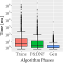
(a) GitHub collection.

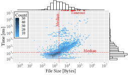
(b) GitHub collection.

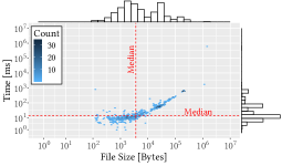
(c) Kubernetes collection.

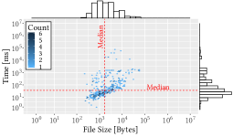
(d) Snowplow collection.

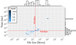
(e) Washington Post collection.

Figure 8. (a) Boxplots of processing times (in milliseconds, log scale) for the 3-phase witness generation algorithm, applied to GitHub schemas. Boxes range from the lower to the upper quartile, horizontal line indicating the median. Whiskers end at the 5th/95th percentile. Outliers above the whiskers are shown as individual dots, darker dots indicate overlapping values. (b-e) Scatterplot showing size of the schema vs. time for generating a witness for the different schema collections. Along top and right edge, a stylized histogram shows the distribution. Top right, the sizes of the files causing timeouts are shown in (b).

9.6.1. Problematic schemas

Our data suggests that a very long runtime does not really depend of the size of the schema but on the presence of specific arrangements of operators.

Our tool fails, with a timeout, only on 40 files, during the phase which interleaves between preparation and DNF. In order to better understand which operator usages create problems to our algorithm, with a focus on those cases where the runtime is definitely too high, we inspected these schemas, and verified that they all feature at least one of the following characteristics:

• object specification with a very long list of properties (reaching 142 for some schema), leading to the object preparation examining a very high number of combinations ;

• string assertions with an argument of $\mathtt{maxLength}$ exceeding $10^{6}$ (Snowplow) or complex pattern expression combined with a relatively high argument for $\mathtt{maxLength}$ (reaching 5,000): both situations lead to manipulating very large automata increasing the total cost of the entire analysis;

• the use if recursive definitions involving the root and a negation of a complex object definition, this entails a problem during object preparation and DNF construction

While these schemas present a tiny portion of the GitHub-crawled corpora, they turn out to be very useful for stress-testing our tool and for indicating optimization opportunities.

9.7. Lessons learned

The experiment was not only useful to verify our hypotheses, but lead us also to other relevant insights, which we summarize here.

9.7.1. Patterns are important

Patterns appear in the $\mathtt{pattern}$ and $\mathtt{patternProperties}$ operators, and can be used to encode operators such as $\mathtt{minLength}$ , $\mathtt{maxLength}$ , and $\mathtt{additionalProperties}$. Since these operators are not extremely common in real-world schemas (see the empirical study in (DBLP:conf/er/BaaziziCGSS21)), it is easy to overlook the practical relevance of patterns in JSON Schema, but we discovered that the high complexity of regular expression operations has noticeable impact on the performance of the algorithm. We now believe that, while it is a good idea to rely on a high-quality external library to deal with the general case, a robust tool for witness generation must also dedicate extra effort to the special cases that arise in this specific application.

9.7.2. Easy schemas are very common

Manual inspection reveals that most GitHub schemas are very simple, using a subset of the operators in a repetitive way, and especially the largest schemas tend to be simplistic, often having been automatically generated (as also observed in (DBLP:conf/er/MaiwaldRS19)). This suggests that the average speed of any tool would greatly benefit from optimization targeted at this specific class of schemas.

9.7.3. Polynomial phases can be relevant

The boxplot shows that the polynomial phases of the algorithm take, on average, more time than the exponential phases. Although we did hope that the exponential phase were manageable, this inversion was for us a surprise, and also a lesson: do not underestimate the phases that appear inexpensive.

9.7.4. $\mathtt{oneOf}$ usually means $\mathtt{anyOf}$

By a manual inspection of the schemas, we discovered that many schema designers define the different branches of a $\mathtt{oneOf}$ to be disjoint, as in

$$\mathtt{\textnormal{\textquotedbl}{oneOf}\textnormal{\textquotedbl}}:[\{\mathtt{\textnormal{\textquotedbl}{type}\textnormal{\textquotedbl}}:\mathtt{\textnormal{\textquotedbl}{null}\textnormal{\textquotedbl}}\},\{\mathtt{\textnormal{\textquotedbl}{type}\textnormal{\textquotedbl}}:\mathsf{\textnormal{\textquotedbl}{string}\textnormal{\textquotedbl}}\}].$$

Hence, the designer is using $\mathtt{oneOf}$ to tell the reader of the schema that the branches are disjoint, but if we substitute that $\mathtt{oneOf}$ with $\mathtt{anyOf}$, the semantics of the schema remains exactly the same. This is extremely relevant, since $\mathtt{oneOf}$ is a very common operator, and $\mathtt{oneOf}$ is much more complex than $\mathtt{anyOf}$, since it requires to compute the conjunction of each branch with the negation of all other branches. We acted upon this observation, and implemented a very simple optimization, where we first rewrite any $\mathtt{oneOf}$ to $\mathtt{anyOf}$, generate a witness for this simplified schema, check the witness against the original schema, and fall back on the complete algorithm only in the extremely rare case when the generated witness was not valid. This simple optimization proved extremely effective.

10. Conclusions

JSON Schema is widely used in data-centric applications. The decidability and complexity of satisfiability and containment were known, but no explicit algorithm had been defined, and it was not obvious whether the high asymptotic complexity of the problem was compatible with a practical algorithm. In this paper we have addressed this open problem. We have described an algorithm for witness generation, satisfiability, and containment, that is based on a specific combination of known and original techniques, to take into account the specific features of JSON Schema object and array operators, and the need to run in a reasonable time.

Our extensive experiments prove the practical viability of the approach, and provide insight into the actual behavior of the algorithm on real-world schemas. These experiments are a necessary step for any redesign or re-factoring of the algorithm.

We have left the implementation of the $\mathtt{uniqueItems}$ operator out of the scope of the current paper in order to keep the size and complexity of this work under control, but the fundamental techniques that we have designed, for object and array preparation and generation, still apply, with some important generalizations that we believe deserve a dedicated analysis.

Acknowledgments

The research has been partially supported by the MIUR project PRIN 2017FTXR7S “IT-MaTTerS” (Methods and Tools for Trustworthy Smart Systems) and by the Deutsche Forschungsgemeinschaft (DFG, German Research Foundation) – 385808805.

We thank Dominik Freydenberger for proposing an algorithm to translate between ECMAScript and Brics REs. We thank Avraham Shinnar for feedback on an earlier version of this paper. We thank Stefan Klessinger for creating the charts and the reproduction package. We thank the students who contributed to our implementation effort: Francesco Falleni, Cristiano Landi, Luca Escher, Lukas Ellinger, Christoph Köhnen, and Thomas Pilz.

References

• (1)
• fak (2022) 2022. JSON Schema Faker. Available on GitHub at https://github.com/json-schema-faker/json-schema-faker and as an interactive tool at https://json-schema-faker.js.org.
• jsv (2022) 2022. JSON schema validator. https://github.com/networknt/json-schema-validator
• onl (2022) 2022. JSONSchemaTool. Available at https://jsonschematool.ew.r.appspot.com.
• rep (2022) 2022. Reproduction Package on GitHub. Temporarily available at GitHub from https://github.com/sdbs-uni-p/JSONSchemaWitnessGeneration, will be moved to Zenodo, for long-term availability.
• Analytics (2022) Snowplow Analytics. 2022. Iglu Central. https://github.com/snowplow/iglu-central, commit hash 726168e.
• Attouche et al. (2021a) Lyes Attouche, Mohamed Amine Baazizi, Dario Colazzo, Yunchen Ding, Michael Fruth, Giorgio Ghelli, Carlo Sartiani, and Stefanie Scherzinger. 2021a. Reproduction package: A Test Suite for JSON Schema Containment. Available on Zenodo at https://zenodo.org/record/5336931#.YshD0XZBxD8 and maintained on GitHub at https://github.com/sdbs-uni-p/json-schema-containment-testsuite.
• Attouche et al. (2021b) Lyes Attouche, Mohamed Amine Baazizi, Dario Colazzo, Yunchen Ding, Michael Fruth, Giorgio Ghelli, Carlo Sartiani, and Stefanie Scherzinger. 2021b. A Test Suite for JSON Schema Containment. In Proc. ER 2021. 19–24. http://ceur-ws.org/Vol-2958/paper4.pdf
• Attouche et al. (2021c) Lyes Attouche, Mohamed Amine Baazizi, Dario Colazzo, Francesco Falleni, Giorgio Ghelli, Cristiano Landi, Carlo Sartiani, and Stefanie Scherzinger. 2021c. A Tool for JSON Schema Witness Generation. In Proc. EDBT 2021. 694–697. https://doi.org/10.5441/002/edbt.2021.86 Tool Demo.
• Attouche et al. (2021d) Lyes Attouche, Mohamed-Amine Baazizi, Dario Colazzo, Francesco Falleni, Giorgio Ghelli, Cristiano Landi, Carlo Sartiani, and Stefanie Scherzinger. 2021d. Un Outil de Génération de Témoins pour les schémas JSON A Tool for JSON Schema Witness Generation. In Proc. Actes de la conférence BDA. Informal proceedings.
• Baazizi et al. (2019a) Mohamed Amine Baazizi, Dario Colazzo, Giorgio Ghelli, and Carlo Sartiani. 2019a. Schemas And Types For JSON Data. In Proc. EDBT. 437–439.
• Baazizi et al. (2019b) Mohamed Amine Baazizi, Dario Colazzo, Giorgio Ghelli, and Carlo Sartiani. 2019b. Schemas and Types for JSON Data: From Theory to Practice. In Proc. SIGMOD Conference. 2060–2063.
• Baazizi et al. (2020) Mohamed-Amine Baazizi, Dario Colazzo, Giorgio Ghelli, Carlo Sartiani, and Stefanie Scherzinger. 2020. Not Elimination and Witness Generation for JSON Schema. In Proc. Actes de la conférence BDA. Informal proceesings, article available online at https://hal.archives-ouvertes.fr/hal-03190106/document.
• Baazizi et al. (2021a) Mohamed Amine Baazizi, Dario Colazzo, Giorgio Ghelli, Carlo Sartiani, and Stefanie Scherzinger. 2021a. An Empirical Study on the ”Usage of Not” in Real-World JSON Schema Documents. In Proc. ER. 102–112. https://doi.org/10.1007/978-3-030-89022-3_9
• Baazizi et al. (2021b) Mohamed Amine Baazizi, Dario Colazzo, Giorgio Ghelli, Carlo Sartiani, and Stefanie Scherzinger. 2021b. A JSON Schema Corpus. A corpus of over 80thousand JSON Schema documents, collected from open source GitHub repositories, using Google BigQuery, in July 2020. Available on Zenodo (10.5281/zenodo.5141199) and maintained on GitHub (https://github.com/sdbs-uni-p/json-schema-corpus).
• Baazizi et al. (2022) Mohamed-Amine Baazizi, Dario Colazzo, Giorgio Ghelli, Carlo Sartiani, and Stefanie Scherzinger. 2022. Negation-Closure for JSON Schema. arXiv:2202.13434 [cs.DB] Accompanying technical report, available online https://arxiv.org/abs/2202.13434.
• Baudart et al. (2020) Guillaume Baudart, Martin Hirzel, Kiran Kate, Parikshit Ram, and Avraham Shinnar. 2020. LALE: Consistent Automated Machine Learning, In Proc. KDD Workshop on Automation in Machine Learning (AutoML@KDD). Computing Research Repository abs/2007.01977. https://arxiv.org/abs/2007.01977
• Blackler (2022) Jim Blackler. 2022. JSON Generator. Available at https://github.com/jimblackler/jsongenerator.
• Bourhis et al. (2017) Pierre Bourhis, Juan L. Reutter, Fernando Suárez, and Domagoj Vrgoc. 2017. JSON: Data model, Query languages and Schema specification. In Proc. PODS. 123–135. https://doi.org/10.1145/3034786.3056120
• Bryant (1986) Randal E. Bryant. 1986. Graph-Based Algorithms for Boolean Function Manipulation. IEEE Trans. Computers 35, 8 (1986), 677–691. https://doi.org/10.1109/TC.1986.1676819
• Comon et al. (2008) Hubert Comon, Max Dauchet, Rémi Gilleron, Florent Jacquemard, Denis Lugiez, Christof Löding, Sophie Tison, and Marc Tommasi. 2008. Tree Automata Techniques and Applications. 262 pages. Available online at https://hal.inria.fr/hal-03367725/file/tata.pdf.
• Corp. (2021) IBM Corp. 2021. jsonsubschema. https://github.com/IBM/jsonsubschema
• Earle et al. (2014) Clara Benac Earle, Lars-Ake Fredlund, Ángel Herranz-Nieva, and Julio Mariño. 2014. Jsongen: a quickcheck based library for testing JSON web services. In Proceedings of the Thirteenth ACM SIGPLAN workshop on Erlang, Gothenburg, Sweden, September 5, 2014, Laura M. Castro and Hans Svensson (Eds.). ACM, 33–41. https://doi.org/10.1145/2633448.2633454
• Freydenberger (2013) Dominik D. Freydenberger. 2013. Extended Regular Expressions: Succinctness and Decidability. Theory Comput. Syst. 53, 2 (2013), 159–193. https://doi.org/10.1007/s00224-012-9389-0
• Fruth et al. (2021) Michael Fruth, Kai Dauberschmidt, and Stefanie Scherzinger. 2021. New Workflows in NoSQL Schema Management. In Proc. SEA-Data@VLDB (CEUR Workshop Proceedings, Vol. 2929). CEUR-WS.org, 38–39.
• Galiegue and Zyp (2013) Francis Galiegue and Kris Zyp. 2013. JSON Schema: interactive and non interactive validation - draft-fge-json-schema-validation-00. Technical Report. Internet Engineering Task Force. https://tools.ietf.org/html/draft-fge-json-schema-validation-00
• Gelade and Neven (2012) Wouter Gelade and Frank Neven. 2012. Succinctness of the Complement and Intersection of Regular Expressions. ACM Trans. Comput. Log. 13, 1 (2012), 4:1–4:19. https://doi.org/10.1145/2071368.2071372
• Gopinath et al. (2021) Rahul Gopinath, Hamed Nemati, and Andreas Zeller. 2021. Input Algebras. In Proc. ICSE. 699–710.
• Habib et al. (2021) Andrew Habib, Avraham Shinnar, Martin Hirzel, and Michael Pradel. 2021. Finding Data Compatibility Bugs with JSON Subschema Checking. In Proc. ISSTA. 620–632. https://doi.org/10.1145/3460319.3464796
• Hopcroft et al. (2007) John E. Hopcroft, Rajeev Motwani, and Jeffrey D. Ullman. 2007. Introduction to automata theory, languages, and computation, 3rd Edition. Addison-Wesley.
• Kubernetes (2022) Kubernetes. 2022. Kubernetes JSON Schemas. https://github.com/instrumenta/kubernetes-json-schema, commit hash 133f848.
• Maiwald et al. (2019) Benjamin Maiwald, Benjamin Riedle, and Stefanie Scherzinger. 2019. What Are Real JSON Schemas Like? - An Empirical Analysis of Structural Properties. In Proc. EmpER@ER, Vol. 11787. Springer, 95–105. https://doi.org/10.1007/978-3-030-34146-6_9
• Møller (2021) Anders Møller. 2021. dk.brics.automaton – Finite-State Automata and Regular Expressions for Java. Available at https://www.brics.dk/automaton/.
• Org (2022a) JSON Schema Org. 2022a. JSON Schema. Available at https://json-schema.org.
• Org (2022b) JSON Schema Org. 2022b. JSON Schema Test Suite. https://github.com/json-schema-org/JSON-Schema-Test-Suite.
• Pezoa et al. (2016) Felipe Pezoa, Juan L. Reutter, Fernando Suárez, Martín Ugarte, and Domagoj Vrgoc. 2016. Foundations of JSON Schema. In Proc. WWW. 263–273. https://doi.org/10.1145/2872427.2883029
• Post (2022) The Washington Post. 2022. ans-schema. https://github.com/washingtonpost/ans-schema, commit hash abdd6c211.
• Stockmeyer (1974) Larry J. Stockmeyer. 1974. The Complexity of Decision Problems in Automata Theory and Logic. Ph. D. Dissertation. Massachusetts Institute of Technology.
• Vahidi (2020) Arash Vahidi. 2020. JDD. https://bitbucket.org/vahidi/jdd/src/master/
• Wright et al. (2019) A. Wright, H. Andrews, and B. Hutton. 2019. JSON Schema Validation: A Vocabulary for Structural Validation of JSON - draft-handrews-json-schema-validation-02. Technical Report. Internet Engineering Task Force. https://tools.ietf.org/html/draft-handrews-json-schema-validation-02
• Wright et al. (2020) A. Wright, H. Andrews, and B. Hutton. 2020. JSON Schema Validation: A Vocabulary for Structural Validation of JSON - draft-bhutton-json-schema-validation-00. Technical Report. Internet Engineering Task Force. https://tools.ietf.org/html/draft-bhutton-json-schema-validation-00
• Wright et al. (2017) A. Wright, G. Luff, and H. Andrews. 2017. JSON Schema Validation: A Vocabulary for Structural Validation of JSON - draft-wright-json-schema-validation-01. Technical Report. Internet Engineering Task Force. https://tools.ietf.org/html/draft-wright-json-schema-validation-01