Perturbative renormalization and thermodynamics of quantum crystalline membranes

Abstract

We analyze the statistical mechanics of a free-standing quantum crystalline membrane within the framework of a systematic perturbative renormalization group (RG). A power-counting analysis shows that the leading singularities of correlation functions can be analyzed within an effective renormalizable model in which the kinetic energy of in-plane phonons and subleading geometrical nonlinearities in the expansion of the strain tensor are neglected. For membranes at zero temperature, governed by zero-point motion, the RG equations of the effective model provide a systematic derivation of logarithmic corrections to the bending rigidity and to the elastic Young modulus derived in earlier investigations. In the limit of a weakly applied external tension, the stress-strain relation at $T=0$ is anomalous: the linear Hooke’s law is replaced with a singular law exhibiting logarithmic corrections. For small, but finite temperatures, we use techniques of finite-size scaling to derive general relations between the zero-temperature RG flow and scaling laws of thermodynamic quantities such as the thermal expansion coefficient $\alpha$, the entropy $S$, and the specific heat $C$. A combination of the scaling relations with an analysis of thermal fluctuations shows that, for small temperatures, the thermal expansion coefficient $\alpha$ is negative and logarithmically dependent on $T$, as predicted in an earlier work. Although the requirement $\lim_{T\to 0}\alpha=0$, expected from the third law of thermodynamics is formally satisfied, $\alpha$ is predicted to exhibit such a slow variation to remain practically constant down to unaccessibly small temperatures.

I Introduction

The statistical mechanics of fluctuating elastic membranes has been investigated extensively over the last decades, in connection with a broad variety of physical systems, from biological layers to graphene and other atomically-thin two-dimensional materials. As it has long been realized, models of flexible surfaces subject to vanishing or small external tension exhibit a rich and striking physical behavior, controlled by an interplay between fluctuations and mechanical nonlinearities [1, 2, 3, 4, 5, 6, 7, 8, 9, 10, 11, 12, 13, 14, 15, 16, 17, 18, 19]. A crucial prediction, in particular, is that for homogeneous free-standing membranes without an imposed stress, anharmonicities inherent in the geometrical definition of the elastic strain tensor are responsible for the stabilization of a macroscopically flat phase at finite temperatures [1, 2, 3, 4], and for a dramatic power-law renormalization of the effective scale-dependent bending rigidity and elastic constants. The presence of a quenched disorder, besides thermal fluctuations, has been predicted to induce an even richer physical behavior [1, 11, 13, 14, 16]. Renormalizations of elastic and thermodynamic properties by ripples have also been analyzed in experiments on graphene membranes [20, 21, 22, 23].

Over the last years, aiming at a more complete theory of fluctuations in graphene, several authors have revisited and extended the analysis by considering the effects of quantization [24, *kats_prb_2014e, 26, 27] and of the coupling between membrane phonons and Dirac electrons [28, 29, 30, 31]. The interaction between flexural and electronic degrees of freedom, in particular, has been predicted to generate mechanical instabilities leading to a spontaneous rippling of the membrane.

Despite the progress in investigations of the coupled membrane-electron problem, the theory of purely mechanical degrees of freedom in a flexible surface subject to both thermal and quantum fluctuations is already highly non-trivial. By a combination of elasticity theory and a one-loop momentum-shell renormalization group, Ref. [24, *kats_prb_2014e] showed that, for a homogeneous and unstressed membrane at absolute zero, mechanical nonlinearities give rise to logarithmic renormalizations of the wavevector-dependent bending stiffness and elastic constants, in sharp contrast with the much stronger power-law renormalizations induced by thermal fluctuations.

In Ref. [26], the theory of quantum flexible membranes was reanalyzed, and extended to the finite temperature case, within the framework of non-perturbative renormalization group (NPRG) techniques. For zero temperature, the weak coupling limit of the NPRG recovers results consistent with the momentum-shell predictions of Ref. [24, *kats_prb_2014e]. At non-zero temperature, the NPRG analysis allowed to smoothly interpolate a crossover between a short wavelength region of zero-point character, and a long-wavelength region, determined by thermal fluctuations. In more detail, the results of Ref. [26] predicted a RG flow exhibiting a first quantum region in which anharmonicities are marginally irrelevant, followed, after a smooth crossover, by a classical region in which nonlinearities are relevant, destabilize the weak coupling approximation, and drive the system to the universal interacting fixed point describing classical thermally-fluctuating membranes [1, 4, 5, 6, 8, 9]. The corresponding correlation functions, in particular, behave in the long-wavelength limit according to the anomalous scaling law characteristic of classical membranes: in the limit of vanishing wavevector $\mathbf{k}\to 0$, the effective bending rigidity diverges as $\kappa(\mathbf{k})\approx k^{-\eta_{*}}$ and the elastic Lamé constant vanish as $\lambda(\mathbf{k}),\mu(\mathbf{k})\approx k^{2-2\eta_{*}}$. A similar picture was derived in Ref. [27], by combining a one-loop RG with a physical approximation: the replacement of the full anharmonic free energy with a Bose-Einstein function with renormalized phonon dispersions. Other field-theoretical analyses on quantum flexible membranes, such as the expansion for large embedding-space dimension and a generalization of the classical self-consistent screening approximation, were developed in Ref. [30], as a part of a wider analysis including the coupling between phonons and Dirac electrons. We finally note that, by different approaches, Refs. [32, 33], have predicted a dynamical behavior qualitatively in contrast with Refs. [24, 25, 26, 27]: that flexural phonon modes acquire a non-zero sound velocity and a linear dispersion relation $\omega(\mathbf{k})\propto|\mathbf{k}|$.

In parallel with analytical approaches, fluctuations of a quantum graphene sheet have also been studied by numerical path-integral simulations based on realistic empirical potentials for interatomic interactions in carbon (see, for example, Ref. [34, 35]).

The objective of this work is to analyze the anharmonic effects in quantum membranes by systematic perturbative renormalization group methods. By a power-counting analysis, we construct an effective renormalizable model which we expect to capture the dominant singularities of physical quantities in the limit of low energies, momenta, temperatures and tensions. At $T=0$, the model is renormalizable in the sense of power counting, although it exhibits anisotropic scaling between space and time, in analogy with other theories with ”weighted power counting” [36, 37, 38, 39, 40, 41]. The corresponding RG equations recover in a systematic framework the earlier results derived in Refs. [24, 25, 26, 27]. We also note that the model is mathematically equivalent to a theory of the decoupled lamellar phase of a three-dimensional stack of classical crystalline membranes analyzed in Ref. [6].

For finite temperatures, we use techniques well-known in the theory of finite size scaling and other finite-temperature field theories [36, 42]. In particular, we use the general property that ultraviolet divergences are temperature-independent and can be renormalized by $T$-independent counterterms [36, 42] to derive scaling laws for various thermodynamic quantities: the thermal expansion coefficient $\tilde{\alpha}$, the entropy $\tilde{S}$, and the specific heat $\tilde{C}$. By combining the scaling relations with an analysis of thermal fluctuations, we recover the result that, for a membrane subject to zero external tension, $\tilde{\alpha}$ is negative and tends to zero in the limit $T\to 0$ as a logarithmic function of $T$, as predicted in Ref. [27].

The effective model and the method used to derive scaling equations are intrinsically focused on the behavior of thermodynamic quantities in the limit of small temperatures. Therefore, the theory developed here cannot capture the detailed $T$ dependence of the thermal expansion coefficient at moderately high temperatures. In particular, the question whether $\tilde{\alpha}$ changes sign at a certain temperature [43, 44, 35, 33], is beyond the scope of this work. We note, however, that the behavior of out-of-plane fluctuations analyzed here contrasts with the prediction of a linear dispersion relation for flexural phonons, which was used in the analyses of Refs. [32, 33].

The coefficient of in-plane thermal expansion of graphene has been estimated by a number of experimental techniques, both for suspended samples and for samples bound to a substrate (see, for example, Refs. [45, 46, 23, 47, 48] and references therein). Experimental results indicate usually a negative thermal expansion at not too large temperatures, although a positive expansion has been identified in Ref. [49] in the case of graphene on a Ir(111) substrate down to liquid helium temperatures.

It would be interesting to test experimentally the prediction of that $\tilde{\alpha}$ is nearly temperature-independent (the logarithmic functions of $T$ change very slowly over broad temperature scales). This prediction applies only to membranes without a supporting substrate and without stress. For a nonzero applied tension, the low-temperature behavior of the thermal expansion coefficient was predicted to vanish in a faster way as $T\to 0$ in Ref. [27].

II Model

To study fluctuations of a quantum membrane, we analyze throughout this work an effective low-energy model defined by the path integral

$${\cal Z}=\int[{\rm d}\mathbf{h}(\mathbf{x},\tau){\rm d}u_{\alpha}(\mathbf{x},\tau)]{\rm e}^{-S/\hbar}$$ (1)

and the imaginary-time action

$$\begin{split}S&[\mathbf{h}(\mathbf{x},\tau),u_{\alpha}(\mathbf{x},\tau)]=\int_{0}^{\hbar/(k_{\rm B}\tilde{T})}{\rm d}\tau\int{\rm d}^{2}x\bigg{\{}\frac{\tilde{\rho}}{2}\dot{\mathbf{h}}^{2}\\ &+\frac{\tilde{\kappa}}{2}(\partial^{2}\mathbf{h})^{2}+\frac{\tilde{\lambda}}{2}(u_{\alpha\alpha})^{2}+\tilde{\mu}u_{\alpha\beta}u_{\alpha\beta}-\tilde{\sigma}\partial_{\alpha}u_{\alpha}\bigg{\}}~{}.\end{split}$$ (2)

The degrees of freedom $u_{\alpha}(\mathbf{x},\tau)$ and $\mathbf{h}(\mathbf{x},\tau)$ represent, respectively, in-plane and out-of-plane displacements of the mass points in the layer. The second line of the action represents the standard elastic energy [1, 2, 17] of a medium with bending rigidity $\tilde{\kappa}$ and Lamé coefficients $\tilde{\lambda}$ and $\tilde{\mu}$, and is defined in terms of the strain tensor $u_{\alpha\beta}=(\partial_{\alpha}u_{\beta}+\partial_{\beta}u_{\alpha}+\partial_{\alpha}\mathbf{h}\cdot\partial_{\beta}\mathbf{h})/2$. The term $-\tilde{\sigma}\partial_{\alpha}u_{\alpha}$ describes an externally applied isotropic in-plane tension [17]. A positive $\tilde{\sigma}>0$ drives a stretching of the membrane, while $\tilde{\sigma}<0$ corresponds to a compressive stress, which tends to buckle the system out of plane. The first term in the action, $\tilde{\rho}\dot{\mathbf{h}}^{2}/2$, describes instead the kinetic energy of out-of-plane fluctuations, and is proportional to the areal mass density $\tilde{\rho}$ and to the square of the out-of-plane velocity $\dot{\mathbf{h}}=\partial\mathbf{h}(\mathbf{x},\tau)/\partial\tau$. Although physically $\mathbf{h}$ is a scalar quantity, we consider in general $\mathbf{h}$ to be a vector with $d_{c}$ components ($d_{c}=1$ for physical membranes embedded in three-dimensional space).

To regularize ultraviolet divergences we implicitly assume a large-momentum cutoff $\Lambda$ of the order of the inverse lattice spacing.

II.1 Rescaled units

By the change of variables $\tau\to(\tilde{\rho}/\tilde{\kappa})^{1/2}\tau$, $\mathbf{h}\to\hbar^{1/2}/(\tilde{\rho}\tilde{\kappa})^{1/4}\mathbf{h}$, $u_{\alpha}\to\hbar/(\tilde{\rho}\tilde{\kappa})^{1/2}u_{\alpha}$, the reduced action $\mathcal{S}=S/\hbar$ can be recast as

$$\begin{split}\mathcal{S}&=\int_{0}^{1/T}{\rm d}\tau\int{\rm d}^{2}x\bigg{\{}\frac{\dot{\mathbf{h}}^{2}}{2}+\frac{1}{2}(\partial^{2}\mathbf{h})^{2}+\frac{\lambda}{2}(u_{\alpha\alpha})^{2}\\ &+\mu u_{\alpha\beta}u_{\alpha\beta}-\sigma\partial_{\alpha}u_{\alpha}\bigg{\}}~{},\end{split}$$ (3)

where $u_{\alpha\beta}=(\partial_{\alpha}u_{\beta}+\partial_{\beta}u_{\alpha}+\partial_{\alpha}\mathbf{h}\cdot\partial_{\beta}\mathbf{h})/2$, $\lambda=\hbar\tilde{\lambda}/(\tilde{\rho}\tilde{\kappa}^{3})^{1/2}$, $\mu=\hbar\tilde{\mu}/(\tilde{\rho}\tilde{\kappa}^{3})^{1/2}$, $T=(\tilde{\rho}/\tilde{\kappa})^{1/2}k_{\rm B}\tilde{T}/\hbar$, and $\sigma=\tilde{\sigma}/\tilde{\kappa}$. After these rescalings, all quantities have a dimension in units of wavevector. The elastic parameters $\lambda$ and $\mu$, which play the role of coupling constants, are dimensionless, while the temperature $T$ and the tension $\sigma$ have the dimension of a wavevector squared.

Throughout the rest of this paper, we always use rescaled units, unless explicitly mentioned. Quantities in standard units of measurements are marked with tilde symbols. The in-plane strain $\tilde{v}$, the Gibbs free energy per unit area $\tilde{\mathcal{G}}=-k_{\rm B}\tilde{T}A^{-1}\ln{\cal Z}$, the entropy density $\tilde{S}=-\partial\tilde{\mathcal{G}}/\partial\tilde{T}$, the specific heat $\tilde{C}=\tilde{T}{\rm d}\tilde{S}/{\rm d}\tilde{T}$, and the thermal expansion coefficient $\tilde{\alpha}=2{\rm d}\tilde{v}/{\rm d}\tilde{T}$, expressed in conventional units, are related to the corresponding rescaled quantities $v$, $\mathcal{G}=-TA^{-1}\ln{\cal Z}$, $S=-\partial\mathcal{G}/\partial T$, $C=T{\rm d}S/{\rm d}T$, $\alpha=2{\rm d}v/{\rm d}T$ as

$$\begin{split}\tilde{v}&=\frac{\hbar v}{(\tilde{\rho}\tilde{\kappa})^{1/2}}~{},\qquad\tilde{\mathcal{G}}=\frac{\hbar\tilde{\kappa}^{1/2}}{\tilde{\rho}^{1/2}}\mathcal{G}~{},\qquad\tilde{S}=k_{\rm B}S\\ \tilde{C}&=k_{\rm B}C~{},\qquad\tilde{\alpha}=k_{\rm B}\alpha/\tilde{\kappa}~{}.\end{split}$$ (4)

II.2 Derivation of the effective model

The effective action (2) can be derived from a more complete theory by a power counting argument. Focusing on the case of a vanishing external tension $\sigma=0$, a more complete model, which includes the kinetic energy of in-plane modes is given by the manifestly rotationally-invariant action [27, 50, 26, 51]

$$\begin{split}S[\mathbf{r}(\mathbf{x},\tau)]&=\int_{0}^{\hbar/(k_{\rm B}\tilde{T})}{\rm d}\tau\int{\rm d}^{2}x~{}\bigg{\{}\frac{\tilde{\rho}}{2}\dot{\mathbf{r}}^{2}+\frac{\tilde{\kappa}}{2}(\partial^{2}\mathbf{r})^{2}\\ &+\frac{\tilde{\lambda}}{2}(U_{\alpha\alpha})^{2}+\tilde{\mu}U_{\alpha\beta}U_{\alpha\beta}\bigg{\}}~{},\end{split}$$ (5)

where $\mathbf{r}\in\mathbb{R}^{d}$ denotes fluctuating coordinates in the $d$-dimensional ambient space and $U_{\alpha\beta}=(\partial_{\alpha}\mathbf{r}\cdot\partial_{\beta}\mathbf{r}-\delta_{\alpha\beta})/2$. This fully rotationally-invariant theory can be analyzed by parametrizing $\mathbf{r}(\mathbf{x},\tau)=(\xi\mathbf{x}+\mathbf{u}(\mathbf{x},\tau),\mathbf{h}(\mathbf{x},\tau))$, where $\mathbf{u}$ and $\mathbf{h}$ are in-plane and out-of-plane displacement fields, while $\xi$ encodes the tendency of the membrane to shrink due to fluctuations [6, 27, 26, 50, 17]. At zero temperature, a loop expansion (formally an expansion in powers of $\hbar$ [36]) can be given by calculating order by order correlation functions and $\xi=1+c_{1}\hbar+c_{2}\hbar^{2}+..$. The non-interacting propagators of in-plane and out-of-plane modes, defining the basic elements in the corresponding diagrammating expansion, are, respectively

$$\begin{split}\bar{D}^{(0)}_{\alpha\beta}(\omega,\mathbf{k})&=\frac{\hbar k_{\alpha}k_{\beta}}{(\tilde{\rho}\omega^{2}+(\tilde{\lambda}+2\tilde{\mu})|\mathbf{k}|^{2}+\tilde{\kappa}|\mathbf{k}|^{4})k^{2}}\\ &+\frac{\hbar(k^{2}\delta_{\alpha\beta}-k_{\alpha}k_{\beta})}{(\tilde{\rho}\omega^{2}+\tilde{\mu}|\mathbf{k}|^{2}+\tilde{\kappa}|\mathbf{k}|^{4})k^{2}}~{},\\ \bar{G}^{(0)}_{ij}(\omega,\mathbf{k})&=\frac{\hbar\delta_{ij}}{\tilde{\rho}\omega^{2}+\tilde{\kappa}|\mathbf{k}|^{4}}~{}.\\ \end{split}$$ (6)

For small $\mathbf{k}$, $\bar{D}^{(0)}_{\alpha\beta}(\omega,\mathbf{k})$ has a pole for $\omega\sim|\mathbf{k}|$ reflecting the linear dispersion of acoustic phonons while $\bar{G}^{(0)}_{\alpha\beta}(\omega,\mathbf{k})$ has a pole for $\omega\sim k^{2}$, corresponding to the ultrasoft dispersion of flexural fluctuations at zero external tension. Due to the softer infrared behavior of flexural phonons, we can assume that poles of $\bar{G}^{(0)}$ generate the leading singularities at long wavelengths. In the region $\omega\sim k^{2}$, interactions can be analyzed within power counting by assigning dimension $[\mathbf{x}]=-1$ to the spacial coordinates and $[\tau]=-z=-2$ to the time coordinate [26] (see Refs. [37, 38, 39, 40, 41] for discussions of of various field theories which lack Lorentz and Euclidean invariance and which exhibit ”weigthed power counting”, with different weigth for space and time coordinates). The behavior of propagators for $\mathbf{k}\to 0$, $\omega\to 0$, $\omega\sim k^{2}$ implies that the canonical dimensions of fields are, respectively, $[\mathbf{h}]=(2+z-4)/2=0$ and $[u_{\alpha}]=(2+z-2)/2=1$. An analysis of dimensions of operators then shows that the elastic parameters $\lambda$ and $\mu$ are marginal, whereas the term $\tilde{\kappa}(\partial^{2}u_{\alpha})^{2}/2$, the nonlinear contribution $\partial_{\alpha}u_{\gamma}\partial_{\beta}u_{\gamma}$ to the strain tensor $U_{\alpha\beta}=((\xi^{2}-1)\delta_{\alpha\beta}+\xi\partial_{\alpha}u_{\beta}+\xi\partial_{\beta}u_{\alpha}+\partial_{\alpha}\mathbf{h}\cdot\partial_{\beta}\mathbf{h}+\partial_{\alpha}u_{\gamma}\partial_{\beta}u_{\gamma})/2$, and the in-plane kinetic energy $\tilde{\rho}\dot{u}_{\alpha}^{2}/2$ are all irrelevant in the sense of power counting. By dropping all power-counting irrelevant interactions, we arrive, after a change of variables $u_{\alpha}\to u_{\alpha}/\xi-(\xi^{2}-1)x_{\alpha}/(2\xi)$, to the effective model (2) with $\sigma=0$.

Clearly, the effective model cannot describe the dynamics of in-plane phonons, which occurs at scales $\omega\sim|\mathbf{k}|$. Power counting indicates however that it should capture in an exact way the leading singularities at long wavelengths of static correlation functions (diagrams with all external frequencies $\omega=0$), and more generally, singularities of diagrams with external legs in the region $\omega\sim k^{2}$ [52], relevant for the behavior of flexural phonons.

For simplicity, we will use the effective model (2) also to calculate thermodynamical properties of the membrane, such as the entropy and the average projected area, at finite temperature $T$ and nonzero tension $\sigma$. We expect that the theory describes the leading singular behavior of thermodynamic quantities for small $T$ and $\sigma$ [53].

As a further remark, we note that, the theory (2) describes only the contribution to thermodynamic quantities of membrane-type fluctuations. In crystal lattices the thermal expansion coefficient and other thermodynamic quantities receive additional contributions from the temperature dependence of the interatomic bond length. We expect that these effects are suppressed at small $T$ and do not contribute to the dominant low-temperature singularities. Within a quasi-harmonic theory, the Grüneisen parameters associated with optical and acoustic in-plane phonons can be assumed to remain finite for $T\to 0$ and $\sigma\to 0$ [7]. Thus we can estimate that the effects of a temperature dependent bond length vanishes at low temperatures proportionally to the specific heat of these phonon branches [7]. By contrast, the fluctuation modes considered here generate infrared singularities, and, as shown in Ref. [27] and discussed below, produce a contribution to the thermal expansion which remains almost constant as $T\to 0$.

II.3 Symmetries

In full analogy with the theory of classical membranes, it can be checked that, when $\sigma=0$, $\mathcal{S}$ is invariant under the ”linearized rotations” [4, 6, 38]

$$\begin{split}\mathbf{h}&\to\mathbf{h}+\mathbf{A}_{\alpha}x_{\alpha}~{},\\ u_{\alpha}&\to u_{\alpha}-(\mathbf{A}_{\alpha}\cdot\mathbf{h})-\frac{1}{2}(\mathbf{A}_{\alpha}\cdot\mathbf{A}_{\beta})x_{\beta}~{},\end{split}$$ (7)

where $\mathbf{A}_{\alpha}$ is any fixed vector. This symmetry represents a linearized form of the original SO($d$) invariance of the full theory, and reflects the fact that the layer is located in an isotropic ambient space (without external forces and with no externally-imposed in-plane tension). The associated Ward identities [4, 6, 38] play a crucial role in the dynamics and the renormalization of the model.

As a remark, we note that the linearized invariance (7) only emerges when all irrelevant terms are dropped from the action at the same time. If, instead, we had neglected the nonlinear contribution $\partial_{\alpha}u_{\gamma}\partial_{\beta}u_{\gamma}/2$ to the strain tensor but we had kept the kinetic energy of in-plane phonons $\tilde{\rho}\dot{u}_{\alpha}^{2}/2$, we would have arrived at a theory which lacks both the full rotational SO$(d)$ symmetry and the linearized, effective rotational symmetry (7). In this case, renormalization would generate generic anisotropic interactions, including anisotropies which are relevant in the sense of power counting. This would then result in an artificial modification of the qualitative behavior of fluctuations. Although the crucial role of symmetries has been appreciated, several approaches in the earlier literature used actions or approximations which, in some steps of derivations, violate both the exact and the linearized SO$(d)$ symmetries.

In particular, we note that the prediction of a contribution $\Sigma(0,\mathbf{k})\propto k^{2}$ to the self-energy of flexural phonons at zero frequency, derived in Ref. [32], started from an action in which the nonlinear contribution to the strain tensor was neglected but the kinetic energy of in-plane phonons was retained. An explicit calculation using a full rotationally-invariant action [27] showed instead that self-energy corrections proportional to $k^{2}$ vanish in absence of external stress, consistently with the Ward identities [50]. The emergence of the linearized symmetry (7) ensures that the cancellation of terms proportional to $k^{2}$ is consistently captured by the effective model (3), as we verify below (see Sec. VI.1).

II.4 Analogy with a model of lamellar phases

After identification of the imaginary time $\tau$ with an additional space dimension $z$, the quantum action $\mathcal{S}$ turns out to be almost identical to the effective Hamiltonian

$$\begin{split}H&=\int{\rm d}z\int{\rm d}^{2}x\bigg{\{}\frac{B_{0}}{2}(\partial_{z}u_{z})^{2}+\frac{K_{0}}{2}(\partial_{\perp}^{2}u_{z})^{2}\\ &+\frac{\mu_{0}^{\perp\perp}}{4}(\partial_{\alpha}u_{\beta}+\partial_{\beta}u_{\alpha}+\partial_{\alpha}u_{z}\partial_{\beta}u_{z})^{2}\\ &+\frac{\lambda_{0}^{\perp\perp}}{8}(2\partial_{\alpha}u_{\alpha}+\partial_{\alpha}u_{z}\partial_{\alpha}u_{z})^{2}+\\ &+\frac{1}{2}\lambda^{\perp z}_{0}(\partial_{z}u_{z})(2\partial_{\alpha}u_{\alpha}+\partial_{\alpha}u_{z}\partial_{\alpha}u_{z})\bigg{\}}~{},\end{split}$$ (8)

which was analyzed by Guitter [38] as a model for a three-dimensional shearless stack of classical crystalline membranes. The identity between the two theories only emerges after irrelevant interactions are neglected in both models and under the assumption $\lambda^{\perp z}_{0}=0$.

The theory of shearless stacks of membranes has been a subject of debate and some authors [54, 55] have proposed models which differ from Eq. (8) and thus contrast with the results of Ref. [38]. Establishing a detailed relation between lamellar phases and quantum membranes is beyond the scope of our work. We will verify, however, that the RG equations for the quantum membrane action recovers long-wavelength singularities identical to those predicted in Ref. [38].

III Integration over in-plane modes

Since $\mathcal{S}$ is quadratic in $u_{\alpha}$, the in-plane modes can be integrated out explicitly. To integrate out $u_{\alpha}$ it is essential to separate the strain tensor $u_{\alpha\beta}$ into uniform modes (with zero spacial momentum $\mathbf{k}=0$) and non-uniform components (with spacial Fourier components $\mathbf{k}\neq 0$). Integration over in-plane phonon modes $u_{\alpha}^{\mathbf{k}\neq 0}(\mathbf{x},\tau)$ with $\mathbf{k}\neq 0$ gives rise to an effective four-point vertex [30]

$$\mathcal{S}^{\mathbf{k}\neq 0}_{\rm int}=\frac{Y}{8}\int_{0}^{1/T}{\rm d}\tau\sum_{\mathbf{k}\neq 0}P^{T}_{\alpha\beta}(\mathbf{k})P^{T}_{\gamma\delta}(\mathbf{k})f_{\alpha\beta}(\mathbf{k},\tau)f_{\gamma\delta}(-\mathbf{k},\tau)~{},$$ (9)

where $f_{\alpha\beta}(\mathbf{k},\tau)$ is the spacial Fourier transform of the composite field $f_{\alpha\beta}(\mathbf{x},\tau)=(\partial_{\alpha}\mathbf{h}(\mathbf{x},\tau)\cdot\partial_{\beta}\mathbf{h}(\mathbf{x},\tau))$, $P^{T}_{\alpha\beta}(\mathbf{k})=\delta_{\alpha\beta}-k_{\alpha}k_{\beta}/k^{2}$ is the projector transversal to the momentum transfer $\mathbf{k}$, and $Y=4\mu(\lambda+\mu)/(\lambda+2\mu)$ is the (dimensionless) Young modulus. The interaction (9) represents physically an instantaneous long-range coupling between local Gaussian curvatures in the membrane, and is a direct quantum generalization of the usual effective interaction which emerges in classical theories [1, 2, 4, 13, 50, 17].

The analysis of zero modes differs depending on the ensemble considered (see Ref. [17] for an analysis of isometric and isotensional ensemble in the theory of classical membranes). Here, we find it convenient to use a fixed-stress, or ”isotensional” ensemble [17], in which the external in-plane stress $\sigma$ is kept fixed and the projected area is allowed to fluctuate. In this setting, we parametrize $u_{\alpha}(\mathbf{x},\tau)=v_{\alpha\beta}x_{\beta}+u^{\mathbf{k}\neq 0}_{\alpha}(\mathbf{x},\tau)$ and integrate over all values of both $u^{\mathbf{k}\neq 0}_{\alpha}(\mathbf{x},\tau)$ and $v_{\alpha\beta}$. After integration, we are lead to a contribution to the effective action

$$\int_{0}^{1/T}{\rm d}\tau\int{\rm d}^{2}x\bigg{[}\frac{\sigma}{2}(\partial_{\alpha}\mathbf{h}\cdot\partial_{\alpha}\mathbf{h})-\frac{\sigma^{2}}{2(\lambda+\mu)}\bigg{]}+\mathcal{S}^{\mathbf{k}=0}_{\rm int}~{},$$ (10)

where

$$\begin{split}\mathcal{S}^{\mathbf{k}=0}_{\rm int}&=A\int_{0}^{1/T}{\rm d}\tau\bigg{[}\frac{\lambda}{8}(f^{0}_{\alpha\alpha}(\tau)-\bar{f}^{0}_{\alpha\alpha})^{2}\\ &+\frac{\mu}{4}(f^{0}_{\alpha\beta}(\tau)-\bar{f}_{\alpha\beta}^{0})(f^{0}_{\alpha\beta}(\tau)-\bar{f}_{\alpha\beta}^{0})\bigg{]}~{},\end{split}$$ (11)

$f^{0}_{\alpha\beta}(\tau)=A^{-1}\int{\rm d}^{2}x(\partial_{\alpha}\mathbf{h}(\mathbf{x},\tau)\cdot\partial_{\beta}\mathbf{h}(\mathbf{x},\tau))$, and $\bar{f}^{0}_{\alpha\beta}=T\int_{0}^{1/T}{\rm d}\tau f^{0}_{\alpha\beta}(\tau)$. The average strain of the membrane in this ensemble is $\langle v_{\alpha\beta}\rangle=v\delta_{\alpha\beta}$, with $v=\sigma/(2(\lambda+\mu))-\langle\partial_{\alpha}\mathbf{h}\cdot\partial_{\alpha}\mathbf{h}\rangle/4$ [11, 50, 17]. It is the sum of a Hookean contribution $\sigma/(2(\lambda+\mu))$, controlled by the bulk modulus $B=\lambda+\mu$, and a negative fluctuation term, proportional to $\langle\partial_{\alpha}\mathbf{h}\cdot\partial_{\alpha}\mathbf{h}\rangle$, which is nonvanishing also for $\sigma=0$, and which represents the tendency of the projected in-plane area to contract due to statistical fluctuations of the layer in the out-of-plane direction.

The infinite-range interaction $\mathcal{S}^{\mathbf{k}=0}_{\rm int}$ is scaled by an overall factor $A^{-1}$ and, by its definition, it vanishes when the Matsubara-frequency transfer between the composite operators $f_{\alpha\beta}^{0}(\tau)$ is zero. These two facts together imply that, in the thermodynamic limit $A\to\infty$, $\mathcal{S}^{\mathbf{k}=0}_{\rm int}$ only contributes via diagrams of the type

(12)

which (a) become disconnected when any zero-mode interaction line (represented by dashed lines) is cut and (b) have non-zero frequency transfer through all dashed lines. (The interaction $\mathcal{S}^{\mathbf{k}\neq 0}_{\rm int}$, denoted by wiggly lines can enter, instead, in arbitrary topology without suppressing the graphs). The diagrams (12), however, are only relevant for zero-mode correlation functions at finite frequency transfer and never enter as subgraphs of other correlation functions. For subsequent calculations in this work, we can thus safely neglect $\mathcal{S}^{\mathbf{k}=0}_{\rm int}$.

As a result, we can thus consider an effective theory for $\mathbf{h}$ fluctuations of the form:

$$\begin{split}\mathcal{S}_{\rm eff}&=\int_{0}^{1/T}{\rm d}\tau\int{\rm d}^{2}x\bigg{\{}\frac{\dot{\mathbf{h}}^{2}}{2}+\frac{1}{2}(\partial^{2}\mathbf{h})^{2}\\ &+\frac{\sigma}{2}(\partial_{\alpha}\mathbf{h})^{2}-\frac{\sigma^{2}}{2B}\bigg{\}}+\mathcal{S}^{\mathbf{k}\neq 0}_{\rm int}~{}.\end{split}$$ (13)

By a Hubbard-Stratonovich decoupling of the long-range interaction [56], the model can be expressed equivalently via the local action

$$\begin{split}\mathcal{S}_{\rm eff}&=\int_{0}^{1/T}{\rm d}\tau\int{\rm d}^{2}x\bigg{\{}\frac{\dot{\mathbf{h}}^{2}}{2}+\frac{1}{2}(\partial^{2}\mathbf{h})^{2}+\frac{\sigma}{2}(\partial_{\alpha}\mathbf{h})^{2}\\ &+\frac{1}{2Y}(\partial^{2}\chi)^{2}+i\chi K-\frac{\sigma^{2}}{2B}\bigg{\}}~{},\end{split}$$ (14)

where $\chi(\mathbf{x},\tau)$ is a mediator field and $K(\mathbf{x},\tau)=(\partial^{2}\mathbf{h}\cdot\partial^{2}\mathbf{h}-\partial_{\alpha}\partial_{\beta}\mathbf{h}\cdot\partial_{\alpha}\partial_{\beta}\mathbf{h})/2$ is, for small fluctuations, the local Gaussian curvature. The term $-\sigma^{2}/(2B)$ is a constant independent of the fluctuating fields $\mathbf{h}$, $\chi$, and does not contribute to statistical averages. The only coupling constant in the model is thus the Young modulus $Y$.

By construction, the interaction-mediating field $\chi$ must be considered as a field with Fourier components only at nonzero momentum $\mathbf{k}\neq 0$. This implies that the tadpole graphs

(15)

must be removed from the perturbative expansion, as in the theory of classical membranes [5].

IV Renormalization and RG equations at zero temperature

IV.1 RG for correlation functions

At $T=0$ the model is infinite in both spacial and temporal dimensions, and its renormalization can proceed in analogy with other bulk theories with weighted power counting [36, 37, 38, 39, 40, 41]. In the representation (14), the basic elements defining diagrams in perturbation theory are the bare propagators of $\mathbf{h}$ and $\chi$,

$$\begin{split}&\includegraphics[scale={1}]{propagator-h}\\ &\includegraphics[scale={1}]{propagator-chi}\\ \end{split}$$ (16)

and the vertex

$$\begin{split}\gamma(\mathbf{k}_{1},\mathbf{k}_{2},\mathbf{k}_{3})&=k_{1}^{2}k_{2}^{2}-(\mathbf{k}_{1}\cdot\mathbf{k}_{2})^{2}=k_{2}^{2}k_{3}^{2}-(\mathbf{k}_{2}\cdot\mathbf{k}_{3})^{2}\\ &=k_{3}^{2}k_{1}^{2}-(\mathbf{k}_{3}\cdot\mathbf{k}_{1})^{2}~{}.\end{split}$$ (17)

The behavior of Feynman integrals under the rescaling $\mathbf{k}\to\lambda\mathbf{k}$, $\omega\to\lambda^{z}\omega=\lambda^{2}\omega$ shows that the weighted power-counting dimension [39] of a one-particle irreducible (1PI) diagram with $I$ internal lines, $V$ vertices, and $L$ loops is $(2+z)L-4I+4V=4(L-I+V)=4$, independently of the order of perturbation theory. This ensures that the model is power-counting renormalizable. A potential danger for renormalizability [40] is that the propagator $F^{(0)}(\omega,\mathbf{k})$, being $\omega$-independent, is not suppressed in the limit $\omega\to\infty$ at $\mathbf{k}$ fixed. However, this does not create difficulties, because it can be checked that in any diagram, all frequency integrals can be performed first and are convergent [57].

To complete the proof of renormalizability, it would be necessary to derive a generalization of the Weinberg theorem [58, 59], ensuring the equivalence between power-counting convergence and true convergence in multiloop diagrams. We will assume that this property remains valid in the model considered in this work.

The ultraviolet divergences of correlation functions can be removed by introducing an arbitrary subtraction scale $M$, a renormalized coupling $Y_{\rm R}$, and a renormalized action

$$\begin{split}\mathcal{S}_{\rm eff}^{\rm(R)}&=\int{\rm d}\tau\int{\rm d}^{2}x\bigg{\{}\frac{\dot{\mathbf{h}}^{2}}{2}+\frac{Z}{2}(\partial^{2}\mathbf{h})^{2}+\frac{\sigma}{2}(\partial_{\alpha}\mathbf{h})^{2}\\ &+\frac{1}{2K_{Y}}(\partial^{2}\chi)^{2}+i\chi K-\frac{\sigma^{2}}{2B}\bigg{\}}~{},\end{split}$$ (18)

equipped with two logarithmically divergent counterterms $Z(Y_{\rm R},\Lambda/M)$ and $K_{Y}(Y_{\rm R},\Lambda/M)$. This particularly simple form, with only two independent divergences, follows from the fact that the terms $\dot{\mathbf{h}}^{2}/2$, $\sigma(\partial_{\alpha}\mathbf{h})^{2}/2$, and the interaction $i\chi K$ are not renormalized. Indeed, due to the structure of the vertex (17), it is possible to factorize, from any 1PI diagram, two powers of the spacial momentum of each external leg. Therefore, the perturbative corrections to the self-energy of flexural fields cannot generate divergences proportional to $\omega^{2}$ or to $k^{2}$, but only proportional to $k^{4}$, which contribute to the renormalization of $Z$. The possibility to factorize two powers of each external momentum also implies that loop corrections to the three-field vertex are superficially convergent, and thus the interaction $i\chi K$ does not require an independent counterterm. An identical mechanism occurs in the $\varepsilon$-expansion of classical membranes in dimension $D=4-\varepsilon$ [13, 56]. In principle, the one-point function $\langle\partial^{2}\chi\rangle$ constitutes a further independent divergence, but since $\chi$ is a field with components only at nonzero momentum $\mathbf{k}\neq 0$, this divergence is unphysical and has no effect on correlation functions.

Eq. (18) implies the following relations between bare and renormalized quantities

$$\begin{split}&\mathcal{S}_{\rm eff}[\mathbf{h},\chi,Y,\sigma]=\mathcal{S}_{\rm eff}^{({\rm R})}[\mathbf{h}_{\rm R},\chi_{\rm R},Y_{\rm R},\sigma_{\rm R}]+\text{constant}~{},\\ &\mathbf{h}(\mathbf{x},\tau)=Z^{1/4}\mathbf{h}_{\rm R}(\mathbf{x},\tau_{\rm R})~{},\qquad\chi(\mathbf{x},\tau)=Z^{-1}\chi_{\rm R}(\mathbf{x},\tau_{\rm R})~{},\\ &\tau=Z^{1/2}\tau_{\rm R}~{},\qquad\sigma=Z^{-1}\sigma_{\rm R}~{},\qquad Y=Z^{-3/2}K_{Y}\end{split}$$ (19)

and, according to standard techniques [36], the following RG equations for 1PI correlation functions in momentum space

$$\begin{split}&\bigg{[}\Lambda\frac{\partial}{\partial\Lambda}+\beta(Y)\frac{\partial}{\partial Y}-\frac{1}{2}(n-4\ell+2)\eta+\eta\sum_{i=1}^{n}\omega_{i}\frac{\partial}{\partial\omega_{i}}\\ &+\eta\sum_{j=1}^{\ell}\omega^{\prime}_{j}\frac{\partial}{\partial\omega^{\prime}_{j}}+2\eta\sigma\frac{\partial}{\partial\sigma}\bigg{]}\Gamma^{(n,\ell)}_{i_{1}..i_{n}}(\omega_{i},\mathbf{k}_{i};\omega^{\prime}_{j},\mathbf{k}^{\prime}_{j})=0~{}.\end{split}$$ (20)

In Eq. (20), $\Lambda$ is the microscopic ultraviolet momentum cutoff and $\Gamma^{(n,\ell)}$ denotes the bare (unrenormalized) 1PI correlation function with $n$ external $\mathbf{h}$ legs and $\ell$ external $\chi$ legs. The RG flow function $\beta=\Lambda\partial Y/\partial\Lambda$ and the anomalous dimension $\eta=-\frac{1}{2}\Lambda\partial\ln Z/\partial\Lambda$ depend only on the bare dimensionless coupling $Y$.

By an explicit computation of the one-loop divergences in the self-energies of $\chi$ and of $\mathbf{h}$ for $\sigma=0$ we find [24, 30, 27]

$$\begin{split}&\includegraphics[scale={1}]{sigma-h}\\ &\includegraphics[scale={1}]{sigma-chi}\\ \end{split}$$ (21)

where $d_{c}=(d-2)$ is the number of components of the $\mathbf{h}$ field. Applying the RG equations to $G_{ij}^{-1}(\omega,\mathbf{k})=\Gamma^{(2,0)}_{ij}(\omega,\mathbf{k})=\omega^{2}+k^{4}+\sigma k^{2}+\Sigma^{(\mathbf{h})}(\omega,\mathbf{k})$ and $F^{-1}(0,\mathbf{k})=\Gamma^{(0,2)}(0,\mathbf{k})=k^{4}/Y+\Sigma^{(\chi)}(0,\mathbf{k})$ shows that, at leading order,

$$\beta(Y)=3\eta(Y)Y+\frac{3d_{c}}{128\pi}Y^{2}~{},\qquad\eta(Y)=\frac{3}{64\pi}Y~{}.$$ (22)

These RG functions imply that $Y$ is marginally irrelevant: the theory is attracted to weak coupling at large length scales. Eqs. (22) are consistent, in a different scheme, with the earlier perturbative results of Refs. [24, 27] and also with the weak-coupling limit of the nonperturbative RG equations derived in Ref. [26].

IV.2 Gibbs free energy

The Gibbs free energy per unit area at zero temperature, $\mathcal{G}_{0}=-A^{-1}\lim_{T\to 0}(T\ln{\cal Z})$, requires the introduction of additional counterterms to the field-independent part of the action. Since $\sigma$ has power-counting dimension $[\sigma]=2$, the required counterterms in the Lagrangian are a polynomial $a_{0}+a_{1}\sigma+a_{2}\sigma^{2}/2$, where $a_{0}$ diverges as $\Lambda^{4}$, $a_{1}$ as $\Lambda^{2}$, and $a_{2}$ diverges logarithmically. By working within a massless scheme [36, 39], $a_{0}$, $a_{1}$, and $a_{2}$ can be chosen to be independent of the tension $\sigma$.

Taking into account these additional renormalizations, the renormalized action reads

$$\begin{split}&\mathcal{S}^{({\rm R})}_{\rm eff}=\int{\rm d}\tau\int{\rm d}^{2}x\bigg{\{}\frac{\dot{\mathbf{h}}^{2}}{2}+\frac{Z}{2}(\partial^{2}\mathbf{h})^{2}+\frac{\sigma}{2}(\partial_{\alpha}\mathbf{h})^{2}\\ &+\frac{1}{2K_{Y}}(\partial^{2}\chi)^{2}+i\chi K+a_{0}+a_{1}\sigma+\frac{1}{2}(a_{2}-1/B)\sigma^{2}\bigg{\}}~{}.\end{split}$$ (23)

To discuss RG equations it is convenient to separate $\mathcal{G}_{0}=V_{\rm el}+\Delta\mathcal{G}_{0}$, where $V_{\rm el}=-\sigma^{2}/(2B)$ is the elastic Hookean contribution and $\Delta\mathcal{G}_{0}$ is the fluctuation part. The advantage of this separation is that $\Delta\mathcal{G}_{0}$ depends only on the Young modulus $Y$ and not on the bulk modulus $B$.

The fluctuation free energy $\Delta\mathcal{G}^{({\rm R})}_{0}$, calculated using the action (23), is finite for $\Lambda\to\infty$ at fixed $Y_{\rm R}$ and $M$. The physical free energy $\Delta\mathcal{G}_{0}$, computed from the bare action (14) is related to $\Delta\mathcal{G}^{({\rm R})}_{0}$ by

$$\begin{split}Z^{1/2}\Delta\mathcal{G}_{0}(Y,Z^{-1}\sigma,\Lambda)&=\Delta\mathcal{G}_{0}^{({\rm R})}(Y_{\rm R},\sigma,M)\\ &-a_{0}^{\prime}-a_{1}\sigma-\frac{a_{2}}{2}\sigma^{2}~{}.\end{split}$$ (24)

($a_{0}^{\prime}$ differs from $a_{0}$ because it receives contributions from the path-integral measure during the change of variables $\mathbf{h}\to\mathbf{h}_{\rm R}$, $\chi\to\chi_{\rm R}$). The relation (24) and the finiteness of $\Delta\mathcal{G}_{0}^{({\rm R})}$ imply an inhomogeneous RG equation for the physical Gibbs free energy

$$\begin{split}\bigg{[}&\Lambda\frac{\partial}{\partial\Lambda}+\beta(Y)\frac{\partial}{\partial Y}+2\eta\sigma\frac{\partial}{\partial\sigma}-\eta\bigg{]}\Delta\mathcal{G}_{0}(Y,\sigma,\Lambda)\\ &=b_{0}+b_{1}\sigma+\frac{b_{2}}{2}\sigma^{2}~{}.\end{split}$$ (25)

The constants $b_{0}$, $b_{1}$, and $b_{2}$ are independent of $\sigma$ in the massless scheme and cannot depend on the arbitrary subtraction scale $M$. Thus they have the form $b_{0}=\bar{b}_{0}(Y)\Lambda^{4}$, $b_{1}=\bar{b}_{1}(Y)\Lambda^{2}$, and $b_{2}=\bar{b}_{2}(Y)$.

V RG for low-temperature thermodynamic quantities

At finite temperatures, the continuum frequency $\omega$ is replaced by discrete bosonic Matsubara frequencies $\omega_{n}=2\pi Tn$. As a result, even for an infinitesimal $T$, the perturbative expansion at zero tension $\sigma=0$ breaks down due to infrared (IR) divergences. The IR problems arise from the $\omega_{n}=0$ component of the flexural propagator $G^{(0)}_{ij}=\delta_{ij}/(\omega_{n}^{2}+k^{4})$, which induces singularities when integrated over the two-dimensional spacial momenta. The physical origin of these divergences is the following: in the limit $\mathbf{k}\to 0$, the system behaves as a classical membrane [26]. For classical thermal fluctuations, anharmonic effects do not induce logarithmic corrections but, rather, power-law renormalizations [1, 2, 4, 5, 6, 13, 51]. The dramatic power-law singularities of the classical theory cannot be captured by a simple perturbative treatment, but require more detailed solutions, for example within the framework of the self-consistent screening approximation [13], the non-perturbative RG [8, 26], the large-$d$ expansion [3, 51], or the $\varepsilon$-expansion [4, 56, 15, 18, 19].

Similar difficulties emerge in finite-size scaling problems and in other finite-temperature quantum field theories. A standard strategy to bypass the problem of IR singularities consists in integrating out modes with $n\neq 0$ and in deriving an effective field theory for modes with $n=0$, to be solved by more exact methods [36].

The same strategy can be applied to the membrane action (14), with, however, a difference compared to the standard case: since the $\chi$ propagator $F^{(0)}(\omega,\mathbf{k})=Y/k^{4}$ does not depend on the frequency $\omega$, it is singular at small $\mathbf{k}$ not only at $\omega_{n}=0$ but, in fact, for all Matsubara frequencies $\omega_{n}\neq 0$. As a result, subtracting the modes $\omega_{n}=0$ does not introduce an IR cutoff to Feynman diagrams. This property is a consequence of the neglection of the kinetic energy of in-plane phonons. The singularity of $F^{(0)}(\omega,\mathbf{k})$, however, is neutralized by the factors $k^{2}$ attached to the vertices (17) and, therefore, the IR finiteness is still valid.

We can thus proceed as follows: we separate $\mathbf{h}(\mathbf{x},\tau)=\mathbf{h}^{\prime}(\mathbf{x},\tau)+\mathbf{H}(\mathbf{x})$, where $\mathbf{H}(\mathbf{x})=T\int_{0}^{1/T}\mathbf{h}(\mathbf{x},\tau)$ is the mode with zero Matsubara frequency and $\mathbf{h}^{\prime}(\mathbf{x},\tau)$ the sum of all other modes with $\omega_{n}\neq 0$. We then integrate out $\mathbf{h}^{\prime}(\mathbf{x},\tau)$ and all degrees of freedom of $\chi(\mathbf{x},\tau)$ (including the $\omega_{n}=0$ mode of $\chi$). This integration can be performed perturbatively without encountering IR divergences because in all $\mathbf{h}^{\prime}$ propagators the finite frequency $\omega_{n}\neq 0$ provides an IR cutoff and in all $\chi$ propagators the singularity $Y/k^{4}$ of the propagator is compensated by a power $k^{4}$ coming from the vertex (17). Although the singularity of $F^{(0)}(\omega,\mathbf{k})$ does not introduce divergences, it still manifests itself in the fact that the effective theory for $\mathbf{H}(\mathbf{x})$ is highly non-local.

In order to disentangle modes which generate IR singularities from degrees of freedom which generate UV divergences, it is also convenient to separate $\mathbf{H}(\mathbf{x})=\mathbf{H}_{1}(\mathbf{x})+\mathbf{H}_{2}(\mathbf{x})$ into a slowly-varying field $\mathbf{H}_{1}(\mathbf{x})$, with momenta $|\mathbf{k}|<\Lambda_{1}$ and a fast field $\mathbf{H}_{2}(\mathbf{x})$ with momenta in the shell $\Lambda_{1}<|\mathbf{k}|<\Lambda$, where $\Lambda_{1}$ is an arbitrary wavevector scale much smaller than $\Lambda$. Integrating out $\mathbf{h}^{\prime}$, $\chi$, and $\mathbf{H}_{2}$ can be done perturbatively and leaves us with an effective classical Hamiltonian

$$\begin{split}{\cal H}&[\mathbf{H}_{1}(\mathbf{x});Y,\sigma,T,\Lambda,\Lambda_{1}]\\ &=-T\ln\int[{\rm d}\mathbf{h}^{\prime}{\rm d}\mathbf{H}_{2}{\rm d}\chi]{\rm e}^{-\mathcal{S}[\mathbf{H}_{1}+\mathbf{H}_{2}+\mathbf{h}^{\prime},\chi]}~{}.\end{split}$$ (26)

involving only slowly-varying long-wavelength modes.

A crucial observation in the theory of finite-size scaling and other finite-temperature field theories is that the counterterms which make the theory finite at $T=0$ will also formally remove all ultraviolet divergences from observables at nonzero $T$ [36, 42]. It is natural to assume that the same property remains valid for the membrane action. We can thus conclude that if we started from the action

$$\begin{split}&\mathcal{S}^{({\rm R})}_{\rm eff}=\int_{0}^{1/T}{\rm d}\tau\int{\rm d}^{2}x\bigg{\{}\frac{\dot{\mathbf{h}}^{2}}{2}+\frac{Z}{2}(\partial^{2}\mathbf{h})^{2}+\frac{\sigma}{2}(\partial_{\alpha}\mathbf{h})^{2}\\ &+\frac{1}{2K_{Y}}(\partial^{2}\chi)^{2}+i\chi K+a_{0}+a_{1}\sigma+\frac{1}{2}(a_{2}-1/B)\sigma^{2}\bigg{\}}~{},\end{split}$$ (27)

equipped with the same zero-temperature counterterms $Z$, $K_{Y}$, $a_{0}$, $a_{1}$, and $a_{2}$ which appear in Eq. (23), after a perturbative integration over $\mathbf{h}^{\prime}$, $\chi$, and $\mathbf{H}_{2}$, and a final non-perturbative integration over $\mathbf{H}_{1}$ we would arrive at a renormalized Gibbs free energy per unit area $\mathcal{G}^{({\rm R})}=-A^{-1}T\ln{\cal Z}$ which remains finite for $\Lambda\to\infty$.

After separation of $\mathcal{G}=V_{\rm el}+\Delta\mathcal{G}$ into the Hookean part $-\sigma^{2}/(2B)$ and the fluctuation part $\Delta\mathcal{G}$, the physical fluctuation free energy $\Delta\mathcal{G}$, computed from the bare action (14) is related to the renormalized $\Delta\mathcal{G}^{({\rm R})}$ by the equation

$$\begin{split}\Delta\mathcal{G}^{({\rm R})}(Y_{\rm R},\sigma,T,M)&=Z^{1/2}\Delta\mathcal{G}(Y,Z^{-1}\sigma,Z^{-1/2}T,\Lambda)\\ &+a_{0}^{\prime}+a_{1}\sigma+\frac{a_{2}}{2}\sigma^{2}~{}.\end{split}$$ (28)

From Eq. (28) follows an inhomogeneous RG equation for the bare Gibbs free energy:

$$\begin{split}\bigg{[}&\Lambda\frac{\partial}{\partial\Lambda}+\beta(Y)\frac{\partial}{\partial Y}+2\eta\sigma\frac{\partial}{\partial\sigma}\\ &+\eta T\frac{\partial}{\partial T}-\eta\bigg{]}\Delta\mathcal{G}(Y,\sigma,T,\Lambda)=b_{0}+b_{1}\sigma+\frac{b_{2}}{2}\sigma^{2}~{}.\end{split}$$ (29)

In Eq. (29), $\beta(Y)$, $\eta(Y)$, and the coefficients of the inhomogeneous part $b_{0}=\bar{b}_{0}(Y)\Lambda^{4}$, $b_{1}=\bar{b}_{1}(Y)\Lambda^{2}$, and $b_{2}=\bar{b}_{2}(Y)$ are the same RG coefficients which appear in the zero-temperature equation (25) and, in particular, are temperature-independent.

As a remark, we note that the RG equations discussed above, as in any renormalizable theory [36], keep track of all terms which either diverge or remain finite when $\Lambda\to\infty$. Terms which vanish for large cutoff (for example a correction $\sigma/\Lambda^{2}$) are instead neglected. As a result, relations such as Eq. (29) are valid asymptotically when the cutoff $\Lambda$ is much larger than other scales in the problem: $\Lambda\gg\sigma^{1/2}$, $\Lambda\gg T^{1/2}$. In standard units of measurement the condition $\Lambda\gg T^{1/2}$ implies that the temperature $\tilde{T}$ must be much smaller than the Debye temperature of flexural phonons $\tilde{T}_{\rm D}=\hbar\tilde{\kappa}^{1/2}\Lambda^{2}/(\tilde{\rho}^{1/2}k_{\rm B})$.

V.1 RG equation for the effective classical Hamiltonian

More generally, the effective classical Hamiltonian (26) must, by itself, satisfy a renormalization group equation

$$\begin{split}\bigg{[}&\Lambda\frac{\partial}{\partial\Lambda}+\beta(Y)\frac{\partial}{\partial Y}+2\eta\sigma\frac{\partial}{\partial\sigma}+\eta T\frac{\partial}{\partial T}\\ &-\frac{\eta}{2}\int{\rm d}^{2}x~{}\mathbf{H}_{1}(\mathbf{x})\cdot\frac{\delta}{\delta\mathbf{H}_{1}(\mathbf{x})}+\eta\bigg{]}\Delta{\cal H}\\ &=A\bigg{(}b_{0}+b_{1}\sigma+\frac{b_{2}}{2}\sigma^{2}\bigg{)}~{},\end{split}$$ (30)

where $\Delta{\cal H}={\cal H}+A\sigma^{2}/(2B)$ is the fluctuation energy, with the Hookean contribution $AV_{\rm el}=-A\sigma^{2}/(2B)$ subtracted. Eq (30) expresses that the cutoff dependence of ${\cal H}$ is entirely carried by the zero-temperature counterterms $Z$, $K_{Y}$, $a_{0}$, $a_{1}$, $a_{2}$.

For the direct validity of Eq. (30), it is essential that all high-energy modes are integrated out, as in Eq. (26). If, for example, we did not integrate out the large-momentum modes $\mathbf{H}_{2}(\mathbf{x})$ with zero Matsubara frequency, we would have moved some of the UV infinities from the integrated modes to the degrees of freedom yet to be integrated. In this case, ${\cal H}$ would have included additional counterterms [42].

VI Results

In this section, we derive explicit consequences of the RG relations for various statistical and thermodynamic quantities.

VI.1 Two-point correlation functions at $T=0$, $\sigma=0$, $\omega=0$

The interacting Green functions $G_{ij}(\omega,\mathbf{k})$ of the flexural field is the inverse of the 1PI function $\Gamma^{(2,0)}_{ij}(\omega,\mathbf{k})$. For $T=0$, $\sigma=0$, and $\omega=0$, $G_{ij}(0,\mathbf{k})=[\Gamma^{(2,0)}_{ij}(0,\mathbf{k})]^{-1}$ satisfies, as a particular case of Eq. (20), the RG equation

$$\Bigg{[}\Lambda\frac{\partial}{\partial\Lambda}+\beta(Y)\frac{\partial}{\partial Y}-2\eta\Bigg{]}G^{-1}_{ij}(0,\mathbf{k};Y,\Lambda)=0~{}.$$ (31)

The renormalization group equations can be solved, in an usual way [36], by introducing a running coupling $y(\Lambda^{\prime})$ and an amplitude renormalization $z(\Lambda^{\prime})$ which, starting from the initial values $y(\Lambda)=Y$, $z(\Lambda)=1$, evolve with the floating cutoff scale $\Lambda^{\prime}$ according to the flow equations

$$\begin{split}\Lambda^{\prime}\frac{{\rm d}y(\Lambda^{\prime})}{{\rm d}\Lambda^{\prime}}&=\beta(y(\Lambda^{\prime}))~{},\\ \Lambda^{\prime}\frac{{\rm d}\ln z(\Lambda^{\prime})}{{\rm d}\Lambda^{\prime}}&=-2\eta(y(\Lambda^{\prime}))~{}.\end{split}$$ (32)

The one-loop RG flow gives

$$\begin{split}y(\Lambda^{\prime})&=\frac{Y}{1+\frac{3(d_{c}+6)Y}{128\pi}\ln\frac{\Lambda}{\Lambda^{\prime}}}~{},\\ z(\Lambda^{\prime})&=\bigg{[}1+\frac{3(d_{c}+6)Y}{128\pi}\ln\frac{\Lambda}{\Lambda^{\prime}}\bigg{]}^{\theta}=\left(\frac{Y}{y(\Lambda^{\prime})}\right)^{\theta}~{},\end{split}$$ (33)

where $\theta=4/(d_{c}+6)$ is the quantum exponent.

To calculate $G_{ij}(0,\mathbf{k})$, we can integrate the RG flow down to a scale $\Lambda^{\prime}\approx k$. Since $y(\Lambda^{\prime})$ flows to small values as $\Lambda^{\prime}$ is reduced (it is marginally irrelevant), we can use perturbation theory and take the zero-order approximation $G^{-1}_{ij}(0,\mathbf{k};y(\Lambda^{\prime}),\Lambda^{\prime})=k^{4}$. The scaling relation (31) then implies $G_{ij}(0,\mathbf{k};Y,\Lambda)\approx\delta_{ij}/(z(k)k^{4})$. By similar arguments, we find that the two point function $F(0,\mathbf{k})=\langle\chi(0,\mathbf{k})\chi(0,-\mathbf{k})\rangle$ of the auxiliary field $\chi$ scales as $F(0,\mathbf{k})\approx z^{3/2}(k)y(k)/k^{4}$.

The scaling of $G_{ij}(0,\mathbf{k})$ shows that $z(k)$ plays the role of a bending-rigidity renormalization and $z^{3/2}(k)y(k)$ the role of an effective screened Young modulus. Returning to standard units, these results can thus be interpreted as a renormalization of the bending rigidity

$$\tilde{\kappa}\to\tilde{\kappa}_{\rm r}(k)=\bigg{[}1+g_{0}\ln\frac{\Lambda}{k}\bigg{]}^{\theta}\tilde{\kappa}$$ (34)

and of the elastic Young modulus $\tilde{Y}=4\tilde{\mu}(\tilde{\lambda}+\tilde{\mu})/(\tilde{\lambda}+2\tilde{\mu})$

$$\tilde{Y}\to\tilde{Y}_{\rm r}(k)=\bigg{[}1+g_{0}\ln\frac{\Lambda}{k}\bigg{]}^{3\theta/2-1}\tilde{Y}$$ (35)

where

$$g_{0}=\frac{3(d_{c}+6)Y}{128\pi}=\frac{3(d_{c}+6)\hbar\tilde{Y}}{128\pi(\tilde{\rho}\tilde{\kappa}^{3})^{1/2}}$$ (36)

is the ”quantum coupling constant” [27]. The bending rigidity gets stiffened by interactions and scales for $k\to 0$ as $[\ln(\Lambda/k)]^{\theta}$. The Young modulus $Y_{\rm r}(k)$, instead, is softened by fluctuations and behaves in the long-wavelength limit as $[\ln(\Lambda/k)]^{3\theta/2-1}=[\ln(\Lambda/k)]^{-d_{c}/(6+d_{c})}$.

The same behavior has been predicted for quantum membranes in Refs. [27, 26]. An identical logarithmic singularity has also been found, for $d_{c}=1$, by Ref. [38] in the context of lamellar stacks of membranes.

The logarithmic renormalizations induced by quantum fluctuations are nonvanishing at all momenta and do not exhibit any characteristic crossover scale, due to the simple structureless form of the beta function $\beta(Y)\propto Y^{2}$. This contrasts with the anharmonic renormalizations in classical membranes [1, 5, 13, 17, 50], which present a crossover between harmonic behavior for $|\mathbf{k}|\gg q_{G}$ and anomalous power-law scaling for $|\mathbf{k}|\ll q_{G}$. Eqs. (34), (35) are valid at all momenta well below to the cutoff scale ( for $|\mathbf{k}|\approx\Lambda$, the continuum approximation breaks down). Using the explicit expression (35), we can estimate that the momentum scale scale at which the running coupling has reached half of its bare value is approximately $|\mathbf{k}|\approx k_{1}=\Lambda{\rm e}^{-1/g_{0}}$. The momentum scale $k_{1}$, however, does not mark a special point in the $\mathbf{k}$-dependence of correlation functions.

VI.1.1 Ultrasoft scaling of $G^{-1}(0,\mathbf{k})$

From the result $G^{-1}_{ij}(0,\mathbf{k})\approx k^{4}[\ln(\Lambda/k)]^{\theta}$ it follows, in particular, that the ultrasoft behavior $\lim_{\mathbf{k}\to 0}G^{-1}_{ij}(0,\mathbf{k})/k^{2}=0$ characteristic of unstressed membranes is preserved by anharmonic effects. This result is consistent with the general Ward identity $\lim_{\mathbf{k}\to 0}G^{-1}_{ij}(0,\mathbf{k})/k^{2}=\sigma$, which is a consequence of rotational invariance [50] and which, here, can be traced to the linearized rotational symmetry (7) of the effective model (2).

We note, instead, that this limiting behavior contrasts with the derivations in Refs. [32, 33], which proposed that, even in an unstressed membrane, flexural phonons exhibit a finite acoustic sound velocity $v$ and a linear dispersion relation $\omega=v|\mathbf{k}|$ for $\mathbf{k}\to 0$. Within the local elasticity model (without long-range interactions) the linear dispersion relation can only emerge when an external source, such as an in-plane stress, breaks the rotational symmetry explicitly. In the harmonic approximation, this follows from the fact that in a rotationally-invariant, unstressed membrane, a Lagrangian term proportional to $(\partial_{\alpha}\mathbf{h})^{2}/2$ cannot appear individually, but only together with in-plane terms in an overall coupling $\sigma_{A}U_{\alpha\alpha}$ to the strain tensor $U_{\alpha\alpha}=(\partial_{\alpha}\mathbf{r}\cdot\partial_{\alpha}\mathbf{r}-2)/2$. The contribution $\sigma_{A}U_{\alpha\alpha}$ represents a coupling to the change of the total area, rather than the in-plane area [60], and thus it is allowed without breaking the symmetry. However, $U_{\alpha\alpha}$ contains a term linear in $\partial_{\alpha}u_{\alpha}$ and, thus, shifts the equilibrium configuration at which the energy must be expanded. After expansion at the true energy minimum, the sound velocity term must disappear. Indeed, a term linear in $\sigma_{A}U_{\alpha\alpha}$ can always be fully removed from the action by a change of variables $\mathbf{r}\to\zeta\mathbf{r}$ [5], which is allowed for a membrane with free boundaries. After $\zeta$ is chosen in such way that terms linear in $\partial_{\alpha}u_{\alpha}$ disappear, the entire operator $U_{\alpha\alpha}$ drops from the action, showing that the inverse Green function behaves as $G^{(0)-1}_{ij}(0,\mathbf{k})\propto k^{4}$. Beyond the harmonic approximation, the perturbative corrections can be assembled in the effective potential $\Gamma$, generating functional of one-particle irreducible correlation functions, which, by Ward identities, has the same symmetry of the action [36]. Because phonon excitations are gapless, the interacting Green function $G^{-1}_{ij}(0,\mathbf{k})$ can vanish slower than $k^{4}$ as a result of singular diagrammatic contributions which generate a non-analytic dependence on $\mathbf{k}$. However, the rotational symmetry forbids terms regular in $\mathbf{k}$ and proportional to $k^{2}$. For example, the first-order perturbative correction for classical membranes in two dimensions [2, 7] consists in a diagram suppressed by an overall factor $k^{4}$ but multiplied by a singular term $1/k^{2}$ arising from the loop integration. Although formally the contribution vanishes as $k^{2}$, its origin is different from a regular contribution directly proportional to $k^{2}$. Furthermore, the singular first-order term proportional to $k^{2}$ is, in fact, the first contribution to an infrared-divergent series which requires a resummation for example by the self-consistent screening approximation [61, 13], or the $\varepsilon$-expansion [4, 56, 18]. After resummation, the interacting correlation function for classical membranes can be shown to behave as $k^{4-\eta_{*}}$ where $\eta_{*}$ is an universal exponent [4, 61, 13]. The value of $\eta_{*}$ has been computed by several complementary techniques [4, 8, 61, 26, 13, 51, 56, 15, 18, 19] (see also references in [56]) and, despite some scatter between different methods, is usually found to be approximately $\eta_{*}\simeq 0.8$. As a result, the full interacting Green function $G^{-1}$ vanishes faster than $k^{2}$.

The same conclusions hold in presence of the linearized rotational invariance (7), which forces the action to depend on $(\partial_{\alpha}\mathbf{h})^{2}$ only via the linearized strain tensor $u_{\alpha\beta}$. (See Refs. [4, 6, 38] for a discussion of Ward identities). Terms linear in $u_{\alpha\alpha}$ can be fully removed by a change of variables $u_{\alpha}\to u_{\alpha}+\varepsilon x_{\alpha}$, a shift which is automatically performed when integrating over zero modes in the fixed-stress ensemble (see Sec. III).

The prediction of a self-energy correction $\Sigma(\mathbf{k})\approx k^{2}\Lambda^{2}$, derived in Ref. [32], resulted from a theory in which the in-plane kinetic energy was kept but the strain tensor was approximated. This approximation breaks explicitly both the full and the linearized rotational symmetry, leading to a result inconsistent with the Ward identities.

VI.2 Average $\langle\hat{\mathbf{h}}(\mathbf{k})\hat{\mathbf{h}}(-\mathbf{k})\rangle$ at $T=0$

The quantum-mechanical average $\langle\hat{\mathbf{h}}(\mathbf{k})\hat{\mathbf{h}}(-\mathbf{k})\rangle$ is given by the integral $\int{\rm d}\omega/(2\pi)G(\omega,\mathbf{k})$ over all frequencies. The scaling relations (20) and the one-loop approximation imply that $\langle\hat{\mathbf{h}}(\mathbf{k})\hat{\mathbf{h}}(-\mathbf{k})\rangle\approx 1/(z^{1/2}(k)k^{2})$.

VI.3 Anomalous Hooke’s law at $T=0$

The average strain of the membrane $\langle\partial_{\alpha}u_{\beta}\rangle=v\delta_{\alpha\beta}$ can be computed from the thermodynamic relation $v=-\frac{1}{2}(\partial\mathcal{G}/\partial\sigma)$. Thus, it is the sum $v=\sigma/(2B)+\Delta v$ of the Hookean term and the fluctuation part $\Delta v=-\frac{1}{2}(\partial\Delta\mathcal{G}/\partial\sigma)=-\langle(\partial_{\alpha}\mathbf{h})^{2}\rangle/4$. The RG equation (29) for the Gibbs free energy implies that, at zero temperature

$$\begin{split}\bigg{[}&\Lambda\frac{\partial}{\partial\Lambda}+\beta(Y)\frac{\partial}{\partial Y}+2\eta\sigma\frac{\partial}{\partial\sigma}+\eta\bigg{]}\Delta v\\ &=-\frac{1}{2}(\bar{b}_{1}(Y)\Lambda^{2}+\bar{b}_{2}(Y)\sigma)~{}.\end{split}$$ (37)

The inhomogeneous coefficients $\bar{b}_{1}(Y)$ and $\bar{b}_{2}(Y)$ are non-zero already in the non-interacting model, because the Gibbs free energy at $T=0$ (equivalent to the zero-point ground state energy) of free flexural phonons is

$$\begin{split}\Delta\mathcal{G}_{0}&=\frac{d_{c}}{2}\int\frac{{\rm d}^{2}k}{(2\pi)^{2}}\sqrt{k^{4}+\sigma k^{2}}\\ &=C_{0}+\frac{d_{c}}{16\pi}\sigma\Lambda^{2}-\frac{d_{c}}{32\pi}\sigma^{2}\ln\Lambda+\text{finite}~{},\end{split}$$ (38)

and already contains divergences for $\Lambda\to\infty$. Matching Eq. (38) with the RG equation (25), we deduce $\bar{b}_{1}(Y)=d_{c}/(8\pi)+{\rm O}(Y)$ and $\bar{b}_{2}(Y)=-d_{c}/(16\pi)+{\rm O}(Y)$. Taking into account that the expansion of $\beta$ and $\eta$ start, respectively, at orders $Y^{2}$ and at order $Y$, it can be checked that the general solution of the RG equation (37) order by order in $Y$ has the general structure

$$v=v_{0}+\frac{\sigma}{2B}+\sum_{k=0}^{\infty}\sum_{\ell=0}^{k+1}a_{k\ell}\sigma Y^{k}\left(\ln(\Lambda^{2}/\sigma)\right)^{\ell}~{}.$$ (39)

The first term, $v_{0}$, represents the average strain at zero imposed stress, and the second two terms describe the response to external tension.

By solving the RG equation (37) in the leading-logarithm approximation [36] (keeping only the most singular terms, with $\ell=k+1$), we find

$$\begin{split}v-v_{0}&=\frac{\sigma}{2B}+\frac{4\sigma}{3Y}\big{[}(z(\sigma^{\frac{1}{2}}))^{\frac{d_{c}}{4}}-1\big{]}~{},\end{split}$$ (40)

where $z(\sigma^{1/2})$ is the running amplitude defined in Eq. (33), evaluated at scale $\Lambda^{\prime}=\sigma^{1/2}$.

Eq. (40) is consistent, at the leading logarithm level, with results obtained by other methods in Ref. [38, 27], and shows that, even at $T=0$, the stress-strain relation is anomalous. Due to quantum fluctuations of flexural degrees of freedom, the macroscopic bulk modulus $B_{\rm eff}=\frac{1}{2}\partial\sigma/\partial v$ is not a constant, but a slowly-varying function of the applied tension:

$$\frac{1}{B_{\rm eff}(\sigma)}\approx\frac{1}{B}+\frac{8}{3Y}\bigg{[}\bigg{(}1+\frac{3(d_{c}+6)Y}{256\pi}\ln\frac{\Lambda^{2}}{\sigma}\bigg{)}^{\frac{d_{c}}{d_{c}+6}}-1\bigg{]}~{}.$$ (41)

(In Eq. (41) we neglected a contribution from the derivative of $z(\sigma^{1/2})$, which does not contribute to the leading-logarithmic singularities). In the limit of zero tension $\sigma\to 0$, the bulk modulus vanishes as $B_{\rm eff}(\sigma)\approx[\ln(\Lambda^{2}/\sigma)]^{-d_{c}/(d_{c}+6)}$.

The physical origin of this singularity is the same which gives rise to the anomalous Hooke response in classical thermally-fluctuating membranes [6, 11, 22, 50]: for small $\sigma$ the dominant effect of the applied tension is not a stretching of the interatomic distance, but rather a ”flattening” of the distribution of out-of-plane flexural fluctuations. The singularity, in particular, is much weaker than the power-law-divergent anomalous Hooke’s law characteristic of classical thermal fluctuations, derived in Refs. [6, 11, 50].

Similarly to the momentum-dependence of $\tilde{\kappa}(k)$ and $\tilde{Y}(k)$, the stress-strain relation does not exhibit any characteristic crossover, reflecting the simple form of the RG beta function $\beta\propto Y^{2}$. The strain response is thus given by a linear Hooke law corrected by logarithmic factors, for all values of the tension. Eqs. (40) and (41) break down, however, when $\sigma$ reaches the cutoff scale $\sigma\approx\Lambda^{2}$. In conventional units, this corresponds to a value of the tension $\tilde{\sigma}=\tilde{\kappa}\Lambda^{2}$. The contribution of quantized out-of-plane fluctuations dominates over the regular Hookean response only at exponentially suppressed values of the tension $\sigma\ll\sigma_{1}\approx\Lambda^{2}{\rm e}^{-2/g_{0}}$, which for parameters characteristic of graphene and two-dimensional materials (see Sec. VII) corresponds to an unphysically small stress. However, the logarithmic corrections induced by out-of-plane motion are nonzero also at much larger values of the stress, and do not present any qualitative change of behavior near $\sigma=\sigma_{1}$. A crossover is expected, instead, for membranes of finite size, since the linear dimension of the system then provides an independent scale. The infinite-size predictions can be assumed to remain valid for $\sigma\gg l^{-2}$, where $l$ is the characteristic linear size.

VI.4 Consequences of renormalizability on low-temperature thermodynamics

Differentiating Eq. (29) with respect to the temperature $T$, annihilates the inhomogeneous terms $b_{0}+b_{1}\sigma+b_{2}\sigma^{2}/2$, which are temperature-independent. As a result we find a homogeneous renormalization group equation for the entropy per unit area $S=-\partial\mathcal{G}/\partial T|_{\sigma}$:

$$\bigg{[}\Lambda\frac{\partial}{\partial\Lambda}+\beta(Y)\frac{\partial}{\partial Y}+2\eta\sigma\frac{\partial}{\partial\sigma}+\eta T\frac{\partial}{\partial T}\bigg{]}S=0~{},$$ (42)

valid in the limit of small tension $\sigma\ll\Lambda^{2}$ and small temperature $T\ll\Lambda^{2}$. By further differentiation with respect to $T$ and to $\sigma$ we find RG equations for the specific heat at constant tension $C=T\partial S/\partial T|_{\sigma}$ and for the thermal expansion coefficient $\alpha=2\partial v/\partial T|_{\sigma}=\partial S/\partial\sigma|_{T}$:

$$\bigg{[}\Lambda\frac{\partial}{\partial\Lambda}+\beta(Y)\frac{\partial}{\partial Y}+2\eta\sigma\frac{\partial}{\partial\sigma}+\eta T\frac{\partial}{\partial T}\bigg{]}C=0~{},$$ (43)

$$\bigg{[}\Lambda\frac{\partial}{\partial\Lambda}+\beta(Y)\frac{\partial}{\partial Y}+2\eta\sigma\frac{\partial}{\partial\sigma}+\eta T\frac{\partial}{\partial T}+2\eta\bigg{]}\alpha=0~{}.$$ (44)

By using the standard method of characteristics [36], the solutions can be written as

$$\begin{split}S(Y,\sigma,T,\Lambda)&=S(y(\Lambda^{\prime}),z^{-1}\sigma,z^{-1/2}T,\Lambda^{\prime})\\ C(Y,\sigma,T,\Lambda)&=C(y(\Lambda^{\prime}),z^{-1}\sigma,z^{-1/2}T,\Lambda^{\prime})\\ \alpha(Y,\sigma,T,\Lambda)&=z^{-1}\alpha(y(\Lambda^{\prime}),z^{-1}\sigma,z^{-1/2}T,\Lambda^{\prime})~{},\end{split}$$ (45)

where $y(\Lambda^{\prime})$ and $z=z(\Lambda^{\prime})$ are the zero-temperature running couplings introduced in Sec. VI.1.

Some general consequences of the RG equations, however, become more manifest if the solutions are expressed in another well-known form [62]. By rewriting the definitions (32) of the flow of running coupligs in the integral form

$$\ln\frac{\Lambda^{\prime}}{\Lambda}=\varphi(y(\Lambda^{\prime}))-\varphi(Y)~{},\qquad z(\Lambda^{\prime})=\frac{{\rm e}^{f(y(\Lambda^{\prime}))}}{{\rm e}^{f(Y)}}~{},$$ (46)

$$\varphi(x)=\int^{x}\frac{{\rm d}u}{\beta(u)}~{},\qquad f(x)=-2\int^{x}{\rm d}u\frac{\eta(u)}{\beta(u)}~{}.$$ (47)

it can be checked that the dimensionless quantities

$$\begin{split}x_{1}&=\ln\frac{\Lambda^{2}}{T}-\frac{1}{2}f(Y)-2\varphi(Y)~{},\\ x_{2}&=\frac{\sigma}{T}{\rm e}^{\frac{1}{2}f(Y)}~{},\end{split}$$ (48)

are RG-invariant (they do not change under the replacements $\Lambda\to\Lambda^{\prime}$, $Y\to y(\Lambda^{\prime})$, $T\to z^{-1/2}(\Lambda^{\prime})T$, $\sigma\to z^{-1}(\Lambda^{\prime})\sigma$).

Taking into account that $\alpha$ is dimensionless, while $S$ and $C$ have the dimension of an inverse area, the scaling relations can then be written in the form, equivalent to Eq. (45),

$$\begin{split}S(Y,\sigma,T,\Lambda)&=T{\rm e}^{\frac{1}{2}f(Y)}L(x_{1},x_{2})~{},\\ C(Y,\sigma,T,\Lambda)&=T{\rm e}^{\frac{1}{2}f(Y)}M(x_{1},x_{2})~{},\\ \alpha(Y,\sigma,T,\Lambda)&={\rm e}^{f(Y)}N(x_{1},x_{2})~{},\\ \end{split}$$ (49)

where $L$, $M$, and $N$ are fixed functions of two parameters. The thermodynamic relations between $S$, $C$, and $\alpha$ imply

$$\begin{split}M(x_{1},x_{2})&=\bigg{[}1-\frac{\partial}{\partial x_{1}}-x_{2}\frac{\partial}{\partial x_{2}}\bigg{]}L(x_{1},x_{2})~{},\\ N(x_{1},x_{2})&=\frac{\partial L(x_{1},x_{2})}{\partial x_{2}}~{}.\end{split}$$ (50)

The detailed form of the functions $L$, $M$, and $N$ is not fixed by the scaling relations, but requires a full solution of the problem, including an analysis of the long-wavelength degrees of freedom dominated by classical thermal fluctuations. However Eqs. (49), which are general consequences of the renormalizability of the zero-temperature theory, already have a predictive content, even without a full solution of the problem. They imply that, in the region $\sigma\ll\Lambda^{2}$, $T\ll\Lambda^{2}$ thermodynamic quantities depend on the microscopic material parameters $\Lambda$ and $Y$ only via overall scale factors independent of $\sigma$ and $T$.

For example, the form of the thermal expansion coefficient at zero tension

$$\alpha={\rm e}^{f(Y)}N(\ln(\Lambda^{2}/T)-f(Y)/2-2\varphi(Y),0)$$ (51)

implies that, in a logarithmic plot of $\ln\alpha$ vs. $\ln T$, curves corresponding to different materials must have the same shape and differ only by rigid shifts along horizontal and vertical Cartesian axes.

These universality properties express, in the thermodynamical behavior, a standard consequence of renormalizability [62].

VI.5 Finite-temperature thermodynamics of an unstressed membrane: thermal expansion coefficient

A more detailed prediction of the temperature dependence of thermodynamic quantities requires a complete theory of all degrees of freedom, from short-wavelength modes, frozen by quantization, to long-wavelength modes, controlled by thermal fluctuations.

To derive explicit expressions we use a combination of the scaling relations (45) with approximations analogue to those described in Ref. [27].

The theories of Refs. [26, 27] indicate that, for temperatures much smaller than the Debye temperature $\tilde{T}_{\rm D}$, correlation functions exhibit a double crossover between different regimes. For large momenta $|\mathbf{k}|\gg q_{T}$ flexural modes have fluctuations of zero-point character. In an intermediate window of length scales $q_{\rm G}\ll|\mathbf{k}|\ll q_{T}$ the system is expected to exhibit weakly-coupled harmonic fluctuations and a classical statistical distribution. Finally in the long-wavelength region $|\mathbf{k}|\ll q_{\rm G}$, fluctuations become strongly anharmonic and are controlled by the interacting fixed point characteristic of classical membranes [1, 4, 5, 8, 13, 17].

The crossover scale $q_{T}$ separating zero-point from thermally activated regimes, can be estimated [27], as the wavelength at which the zero-temperature inverse Green function $G^{-1}_{ij}(0,\mathbf{k})\approx z(k)k^{4}$ becomes of the order of $T^{2}$:

$$z(q_{T})q_{T}^{4}\simeq T^{2}~{}.$$ (52)

For a fully classical membrane with bending rigidity $\tilde{\kappa}_{1}$, Young modulus $\tilde{Y}_{1}$, and temperature $\tilde{T}_{1}$, the Ginzburg momentum $q_{\rm G}$ at which harmonic fluctuations cross over to strongly-coupled nonlinear fluctuations is [1, 5, 13, 50, 17] $q_{\rm G}\simeq(3k_{\rm B}\tilde{T}_{1}\tilde{Y}_{1}/(16\pi\tilde{\kappa}_{1}^{2}))^{1/2}$. In the quantum problem it can be assumed that the same crossover criterion remains valid, with $\tilde{T}_{1}=\tilde{T}$ and that $\tilde{\kappa}_{1}=\tilde{\kappa}_{\rm r}(q_{T})$, $\tilde{Y}_{1}=\tilde{Y}_{\rm r}(q_{T})$ are the renormalized parameters (34), (35), corrected by zero-point anharmonic effects, evaluated at the renormalization scale $q_{T}$ [27]. In rescaled units, the corresponding crossover scale is

$$q_{G}^{2}\simeq\frac{3Ty(q_{T})}{16\pi(z(q_{T}))^{1/2}}~{}.$$ (53)

With characteristic parameters of graphene (see Sec. VII), it can be verified that $(q_{G}/q_{T})^{2}=3y(q_{T})/16\pi$ is small, confirming the consistency of a region $q_{\rm G}\ll|\mathbf{k}|\ll q_{T}$.

By using Eq. (45), we can estimate the thermal expansion of the quantum membrane as

$$\alpha(Y,T,\Lambda)=(z(q_{T}))^{-1}\alpha(y(q_{T}),z(q_{T})^{-1/2}T,q_{T})~{}.$$ (54)

In principle, the zero-temperature RG flow remains valid only as far as $\Lambda^{\prime}\gg z^{-1/2}(\Lambda^{\prime})T$, but, in a first approximation, it is justified to set directly $\Lambda^{\prime}=q_{T}=z^{-1/2}(q_{T})T$.

After the cutoff has been reduced from the microscopic scale to the thermal scale $q_{T}$, we can estimate $\alpha$ by neglecting quantum thermal effects and by identifying $\alpha(y(q_{T}),z^{-1/2}(q_{T})T,q_{T})$ with the thermal expansion coefficient of a classical membrane with the standard Hamiltonian [1, 2, 5, 27, 26]

$$\begin{split}{\cal H}_{\rm cl}[\mathbf{H}_{1}(\mathbf{x})]&=\int{\rm d}^{2}x\bigg{[}\frac{\kappa_{\rm cl}}{2}(\partial^{2}\mathbf{H}_{1})^{2}\\ &+\frac{Y_{\rm cl}}{8}(P^{T}_{\alpha\beta}(-\partial^{2})(\partial_{\alpha}\mathbf{H}_{1}\cdot\partial_{\beta}\mathbf{H}_{1}))^{2}\bigg{]}~{}.\end{split}$$ (55)

In terms of the discussion of Sec. V, this corresponds to approximating ${\cal H}[\mathbf{H}_{1}]$, the Hamiltonian for modes with zero Matsubara frequency, with Eq. (55), which is its tree-level approximation (without loop corrections).

In particular, we must consider a classical membrane with Young modulus $Y_{\rm cl}=y(q_{T})$, temperature $T_{\rm cl}=z^{-1/2}(q_{T})T$, bending rigidity $\kappa_{\rm cl}=1$, and a large-momentum cutoff $\Lambda_{\rm cl}=q_{T}$.

Thermal fluctuations in classical statistical mechanics have been investigated extensively [1, 2, 5, 50, 13, 56, 51, 15, 17]. The momentum-dependent correlation function $G_{ij}^{({\rm cl})}(\mathbf{k})=\langle h_{i}(\mathbf{k})h_{j}(-\mathbf{k})\rangle$ is predicted to behave as

$$G_{ij}^{({\rm cl})}(\mathbf{k})=\delta_{ij}\begin{cases}\frac{T_{\rm cl}}{\kappa_{\rm cl}k^{4}}~{},&\text{for }q_{\rm G}\ll|\mathbf{k}|\ll\Lambda_{\rm cl}\\ \frac{T_{\rm cl}}{\kappa_{\rm cl}k^{4-\eta_{*}}q_{\rm G}^{\eta_{*}}}&\text{for }|\mathbf{k}|\ll q_{\rm G}~{},\end{cases}$$ (56)

where $\eta_{*}$ is an universal exponent and $q_{G}=(3T_{\rm cl}Y_{\rm cl}/(16\pi\kappa_{\rm cl}^{2}))^{1/2}$.

Calculating directly the extension factor via the relation

$$\begin{split}\langle v_{\rm cl}\rangle&=-\frac{1}{4}\langle(\partial_{\alpha}\mathbf{h})^{2}\rangle=-\frac{1}{4}\int\frac{{\rm d}^{2}k}{(2\pi)^{2}}G_{ii}(\mathbf{k})\\ &\simeq-\frac{d_{c}T_{\rm cl}}{8\pi\kappa_{\rm cl}}\bigg{[}\int_{0}^{q_{\rm G}}\frac{{\rm d}k}{q_{\rm G}^{\eta_{*}}k^{1-\eta_{*}}}+\int_{q_{\rm G}}^{\Lambda_{\rm cl}}\frac{{\rm d}k}{k}\bigg{]}\\ &=-\frac{d_{c}T_{\rm cl}}{8\pi\kappa_{\rm cl}}\bigg{[}\frac{1}{\eta_{*}}+\ln\frac{\Lambda_{\rm cl}}{q_{\rm G}}\bigg{]}\end{split}$$ (57)

and differentiating with respect to $T_{\rm cl}$ at $\Lambda_{\rm cl}$, $Y_{\rm cl}$ and $\kappa_{\rm cl}$ fixed we find the expression for the thermal expansion coefficient [63]

$$\alpha_{\rm cl}=2\frac{\partial\langle v_{\rm cl}\rangle}{\partial T_{\rm cl}}=-\frac{d_{c}}{4\pi\kappa_{\rm cl}}\left[\frac{1}{\eta_{*}}-\frac{1}{2}+\ln\frac{\Lambda_{\rm cl}}{q_{\rm G}}\right]~{}.$$ (58)

Identifying, in rescaled units, $\alpha=(z(q_{T}))^{-1}\alpha_{\rm cl}$, and setting the effective classical parameters to the renormalized values we then find an expression for the thermal expansion coefficient of quantum membranes

$$\alpha=-\frac{d_{c}}{4\pi z(q_{T})}\bigg{[}\frac{1}{\eta_{*}}-\frac{1}{2}+\frac{1}{2}\ln\bigg{(}\frac{16\pi}{3y(q_{T})}\bigg{)}\bigg{]}~{}.$$ (59)

This expression, when $z(q_{T})$ and $y(q_{T})$ are replaced with the one-loop running couplings

$$y(q_{T})=\frac{Y}{1+\frac{3(d_{c}+6)Y}{128\pi}\ln\frac{\Lambda}{q_{T}}}~{},\quad z(q_{T})=\left(\frac{Y}{y(q_{T})}\right)^{\theta}~{},$$ (60)

coincides with the result derived in Ref. [27], up to a numerical factor.

The temperature dependence of $\alpha$ is entirely driven by the renormalization factors $y(q_{T})$ and $z(q_{T})$. As a result, the thermal expansion coefficient is a slow, logarithmic function of $T$. In the limit $T\to 0$, $\alpha$ tends to zero as

$$\alpha_{T}\approx-\frac{d_{c}}{8\pi}\frac{\ln(\ln(\Lambda^{2}/T))}{[(g_{0}/2)\ln(\Lambda^{2}/T)]^{\theta}}~{}.$$ (61)

As a remark, we note that, despite being approximate, the solution (59) is automatically consistent with the general form (51), as it is true for any expression of the type $\alpha=(z(q_{T}))^{-1}F(y(q_{T}))$, constructed via running couplings.

The approximations which lead to Eq. (59) are very natural. We expect that the prediction of a nearly constant $\alpha$ at low temperature is exact and that Eq. (61) captures, up to a numerical factor, the correct behavior in the limit $T\to 0$.

VI.6 Renormalization and third law of thermodynamics

The fact that $\alpha$ vanishes in the zero-temperature limit is formally consistent with the requirement $\lim_{T\to 0}\alpha(T)=0$, which is expected in view of the Maxwell relation

$$\alpha=\left(\frac{\partial V}{\partial T}\right)_{p}=-\left(\frac{\partial S}{\partial p}\right)_{T}~{},$$ (62)

and the third law of thermodynamics $\lim_{T\to 0}S(T,p)=0$ [32, 35, 64]. The logarithmic way in which the low temperature limit is realized at zero tension is, however, very unconventional [27]. In fact, the existence of an anomalous behavior can be already anticipated by dimensional analysis. The rescalings described in Sec. II.1 show that, for $\sigma=0$, the only dimensionful parameters in the theory (3) are the temperature $T$ and the UV cutoff $\Lambda$. If there were no ultraviolet divergences, the fact that $\alpha$ is dimensionless would have implied that $\alpha=\phi(Y)$, a temperature-independent result which is manifestly inconsistent with the limit $\lim_{T\to 0}\alpha(T)=0$. It is only the logarithmic correction due to UV divergences which introduces an explicit dependence on the UV cutoff scale $\Lambda$ and allows for a variation of $\alpha$ at low temperatures. In presence of a nonzero tension $\sigma$, Ref. [27] predicted that the thermal expansion coefficient vanishes in a faster way for $T\to 0$.

VII Application to graphene

To illustrate results, we consider the case of a monolayer graphene, using parameters $\tilde{\rho}\simeq 7.6$ kg m^-2, $\tilde{\lambda}\simeq 3.4$ eV Å^-2, $\tilde{\mu}\simeq 9.3$ eV Å^-2, $\tilde{B}\simeq 12.7$ eVÅ^-2, $\tilde{Y}\simeq$ 21.4 eV Å^-2 [10], $\kappa\simeq 1.4$ eV [65]. Setting the codimension $d_{c}$ to the physical value $d_{c}=1$, we find that the bare value of the quantum coupling constant is small: $g_{0}\simeq 0.02$. As a consequence, the one-loop approximations to the RG functions $\beta$ and $\eta$ are justified at all length scales of physical interest. The smallness of $g_{0}$ is related physically to the fact that the mass of nuclei is much larger than the mass of electrons [24, 25], and, thus, we expect it to be a general feature of most two-dimensional materials.

The ultraviolet cutoff $\Lambda$ is of the order of the inverse interatomic distance $a\simeq 1.42$ Å. We choose to identify $\Lambda$ with the ”Debye radius” $\Lambda=(4\pi^{2}/3)^{1/4}a^{-1}$, defined by the condition that the phase space area $\pi\Lambda^{2}$ contains the same number of degrees of freedom of the hexagonal Brillouin zone of graphene. With this estimate, the Debye temperature is approximately $\tilde{T}_{\rm D}=\hbar(\tilde{\kappa}/\tilde{\rho})^{1/2}\Lambda^{2}/k_{\rm B}\simeq 750$ K.

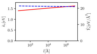
Figure 1: Effective wavevector-dependent bending rigidity (red solid line) and Young modulus (blue dashed line) as a function of wavelength $l=2\pi/k$ for a graphene membrane at $T=0$, as described by Eqs. (34) and (35). In the infinite-wavelength limit $\tilde{\kappa}_{\rm r}(l)$ slowly diverges as $(\ln l)^{4/7}$ and $\tilde{Y}_{\rm r}(l)$ slowly vanishes as $(\ln l)^{-1/7}$.

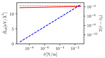
Figure 2: Anomalous Hooke’s law for a graphene membrane at $T=0$. The red solid line represents the macroscopic bulk modulus $\tilde{B}_{\rm eff}=\frac{1}{2}\partial\tilde{\sigma}/\partial\tilde{v}$ as a function of the applied tension $\tilde{\sigma}$, as described by Eq. (41). The red dotted line is constant as a function of the applied stress and identifies the microscopic bulk modulus $\tilde{B}\simeq 12.7$ eV Å^-2 controlling the normal Hooke’s law for a membrane constrained in two dimension (without quantum-mechanical out-of-plane fluctuations). The strain induced by tension is represented by blue dashed lines. The effective bulk modulus vanishes in the limit $\sigma\to 0$ as $\tilde{B}_{\rm eff}(\sigma)\approx(\ln(1/\sigma))^{-1/7}$. The singularity, however, is very slow. The prediction for the stress-strain relation breaks down when the tension is so large that the stress dominates over bending rigidity at all momentum scales up to the cutoff $\Lambda$. Eq. (41) is thus valid for $\tilde{\sigma}\ll\tilde{\kappa}\Lambda^{2}\simeq 40$ N/m.

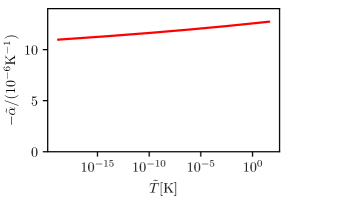
Figure 3: Negative thermal expansion coefficient for an unstressed graphene membrane as a function of temperature (red solid line). In the limit $T\to 0$, $\tilde{\alpha}\to 0$ as expected from the third law of thermodynamics, but the approach to zero is only logarithmic with $\tilde{T}$.

The predictions discussed in Sec. VI are illustrated in figures 1, 2, and 3. In all cases, the renormalizations induced by quantum-mechanical fluctuations induce a slow, logarithmic behavior of statistical and thermodynamic quantities.

In particular, we find that the thermal expansion coefficient $\tilde{\alpha}$ at low temperatures is nearly constant over broad ranges of low temperature, with an order of magnitude $\tilde{\alpha}\approx-k_{\rm B}/(4\pi\tilde{\kappa})\approx-5\times 10^{-6}$ K^-1 up to a numerical factor of order unity, in agreement with a simple classical estimate [63]. The limit $\lim_{T\to 0}\alpha=0$ is only approached logarithmically.

Let us estimate the characteristic crossover scales for flexural fluctuations. At $\tilde{T}=300$ K, the crossover momentum $q_{T}$ between zero-point and classical fluctuations is approximately $q_{T}\simeq 0.9$ Å^-1, corresponding to a wavelength $l_{T}\simeq 7.4$ Å^-1. The Ginzburg length separating harmonic and anharmonic classical regimes is, for $T\simeq 300$ K, approximately $l_{G}=2\pi/q_{G}\simeq 50$ Å. At different temperatures, the characteristic lengths $l_{T}$ and $l_{G}$ are both proportional to $\tilde{T}^{-1/2}$, up to logarithmic factors. This is a manifestation of the scale-invariance of the action, which is only weakly broken by logarithmic renormalization effects.

The prediction of a nearly constant $\tilde{\alpha}$ depends essentially on the fact that flexural phonon modes fluctuate in absence of an imposed stress and without binding forces (see Ref. [27] for an analysis on the role of tension and Refs. [63, 48] for discussions on the effects of a supporting substrate).

To conclude, we note that a more complete understanding of the thermodynamics of graphene samples requires a further analysis of the coupling between membrane fluctuations and Dirac electrons, which have been proposed to be at the origin of mechanical instabilities such as a spontaneous rippling [61, 30]. The role of electron fluctuations, however, is suppressed in insulating 2D materials such as hexagonal boron nitride.

VIII Summary and conclusions

To summarize, we have analyzed the theory of a fluctuating quantum mechanical membrane within the framework of perturbative renormalization group techniques. At zero temperature, the perturbative RG provides a systematic derivation of logarithmic singularities analyzed in earlier investigations by momentum-shell and by nonperturbative renormalization group techniques. In the limit of a weakly applied external tension $\tilde{\sigma}$, we recover the result that the stress-strain relation at $T=0$ is singular: for $\tilde{\sigma}\to 0$, the strain behaves as $\tilde{\sigma}[\ln(1/\tilde{\sigma})]^{-1/7}$.

In the case of a small, but nonzero temperature, techniques of finite-size quantum field theory provide general scaling relations for thermodynamic quantities such as the entropy $S$, the specific heat $C$, and the thermal expansion coefficient $\alpha$ at vanishing or small external tension. By an approximate solution of the theory, we derive that the negative thermal expansion coefficient of an unstressed crystalline membrane vanishes for $T\to 0$ as a logarithmic function of the temperature.

References

- Nelson et al. [2004] D. R. Nelson, T. Piran, and S. Weinberg, eds., Statistical mechanics of membranes and surfaces, 2nd ed. (World Scientific, Singapore, 2004).
- Nelson and Peliti [1987] D. R. Nelson and L. Peliti, J. Physique 48, 1085 (1987).
- David and Guitter [1988] F. David and E. Guitter, EPL 5, 709 (1988).
- Aronovitz and Lubensky [1988] J. A. Aronovitz and T. C. Lubensky, Phys. Rev. Lett. 60, 2634 (1988).
- Aronovitz et al. [1989] J. Aronovitz, L. Golubovic, and T. C. Lubensky, J. Physique 50, 609 (1989).
- Guitter et al. [1989] E. Guitter, F. David, S. Leibler, and L. Peliti, J. Physique 50, 1787 (1989).
- Katsnelson [2020] M. I. Katsnelson, The physics of graphene, 2nd ed. (Cambridge University Press, Cambridge, 2020).
- Kownacki and Mouhanna [2009] J.-P. Kownacki and D. Mouhanna, Phys. Rev. E 79, 040101(R) (2009).
- Košmrlj and Nelson [2016] A. Košmrlj and D. R. Nelson, Phys. Rev. B 93, 125431 (2016).
- Los et al. [2016] J. H. Los, A. Fasolino, and M. I. Katsnelson, Phys. Rev. Lett. 116, 015901 (2016).
- Gornyi et al. [2017] I. V. Gornyi, V. Y. Kachorovskii, and A. D. Mirlin, 2D Mater. 4, 011003 (2017).
- Los et al. [2017] J. H. Los, A. Fasolino, and M. I. Katsnelson, npj 2D Materials and Applications 1, 9 (2017).
- Le Doussal and Radzihovsky [2018] P. Le Doussal and L. Radzihovsky, Ann. Phys. 392, 340 (2018).
- Saykin et al. [2020a] D. R. Saykin, V. Y. Kachorovskii, and I. S. Burmistrov, Phys. Rev. Research 2, 043099 (2020a).
- Coquand et al. [2020] O. Coquand, D. Mouhanna, and S. Teber, Phys. Rev. E 101, 062104 (2020).
- Coquand and Mouhanna [2021] O. Coquand and D. Mouhanna, Phys. Rev. E 103, L031001 (2021).
- Shankar and Nelson [2021] S. Shankar and D. R. Nelson, Phys. Rev. E 104, 054141 (2021).
- Metayer et al. [2022] S. Metayer, D. Mouhanna, and S. Teber, Phys. Rev. E 105, L012603 (2022).
- Pikelner [2021] A. Pikelner, arXiv:2112.073 https://arxiv.org/abs/2112.07340 (2021).
- López-Polín et al. [2015] G. López-Polín, C. Gómez-Navarro, V. Parente, F. Guinea, M. I. Katsnelson, F. Pérez-Murano, and J. Gómez-Herrero, Nat. Phys. 11, 26 (2015).
- Blees et al. [2015] M. K. Blees, A. W. Barnard, P. A. Rose, S. P. Roberts, K. L. McGill, P. Y. Huang, A. R. Ruyack, J. W. Kevek, B. Kobrin, D. A. Muller, and P. L. McEuen, Nature 524, 204 (2015).
- Nicholl et al. [2017] R. J. T. Nicholl, N. V. Lavrik, I. Vlassiouk, B. R. Srijanto, and K. I. Bolotin, Phys. Rev. Lett. 118, 266101 (2017).
- Lopez-Polin et al. [2021] G. Lopez-Polin, C. Gomez-Navarro, and J. Gomez-Herrero, Nano Mater. Sci. 10, 1 (2021).
- Kats and Lebedev [2014] E. I. Kats and V. V. Lebedev, Phys. Rev. B 89, 125433 (2014).
- Kats and Lebedev [2016] E. I. Kats and V. V. Lebedev, Phys. Rev. B 94, 079904(E) (2016).
- Coquand and Mouhanna [2016] O. Coquand and D. Mouhanna, Phys. Rev. E 94, 032125 (2016).
- Burmistrov et al. [2016] I. S. Burmistrov, I. V. Gornyi, V. Y. Kachorovskii, M. I. Katsnelson, and A. D. Mirlin, Phys. Rev. B 94, 195430 (2016).
- Gazit [2009a] D. Gazit, Phys. Rev. B 80, 161406(R) (2009a).
- San-Jose et al. [2011] P. San-Jose, J. González, and F. Guinea, Phys. Rev. Lett. 106, 045502 (2011).
- Guinea et al. [2014] F. Guinea, P. Le Doussal, and K. J. Wiese, Phys. Rev. B 89, 125428 (2014).
- Cea et al. [2020] T. Cea, M. Ruiz-García, L. L. Bonilla, and F. Guinea, Phys. Rev. B 101, 235428 (2020).
- Amorim et al. [2014] B. Amorim, R. Roldán, E. Cappelluti, A. Fasolino, F. Guinea, and M. I. Katsnelson, Phys. Rev. B 89, 224307 (2014).
- Bondarev et al. [2018] V. N. Bondarev, V. M. Adamyan, and V. V. Zavalniuk, Phys. Rev. B 97, 035426 (2018).
- Hašík et al. [2018] J. Hašík, E. Tosatti, and R. Martoňák, Phys. Rev. B 97, 140301(R) (2018).
- Herrero and Ramírez [2016] C. P. Herrero and R. Ramírez, J. Chem. Phys. 145, 224701 (2016).
- Zinn-Justin [2002] J. Zinn-Justin, Quantum field theory and critical phenomena, 4th ed., International series of monographs on physics, Vol. 113 (Oxford University Press, 2002).
- Brézin and Zinn-Justin [1976] E. Brézin and J. Zinn-Justin, Phys. Rev. B 13, 251 (1976).
- Guitter [1990] E. Guitter, J. Physique 51, 2407 (1990).
- Anselmi and Halat [2007] D. Anselmi and M. Halat, Phys. Rev. D 76, 125011 (2007).
- Anselmi [2008] D. Anselmi, J. High Energy Phys. 02, 051.
- Arav et al. [2019] I. Arav, Y. Oz, and A. Raviv-Moshe, J. High Energy Phys. 11, 064.
- Zinn-Justin [2000] J. Zinn-Justin, arXiv:hep-ph/0005272 (2000).
- Zakharchenko et al. [2009] K. V. Zakharchenko, M. I. Katsnelson, and A. Fasolino, Phys. Rev. Lett. 102, 046808 (2009).
- Jiang et al. [2015] J.-W. Jiang, B.-S. Wang, J.-S. Wang, and H. S. Park, J. Phys.: Condens. Matter 27, 083001 (2015).
- Bao et al. [2009] W. Bao, F. Miao, Z. Chen, H. Zhang, W. Jang, C. Dames, and C. N. Lau, Nat. Nanotechnol. 4, 562 (2009).
- Singh et al. [2010] V. Singh, S. Sengupta, H. S. Solanki, R. Dhall, A. Allain, S. Dhara, P. Pant, and M. M. Deshmukh, Nanotechnology 21, 165204 (2010).
- Yoon et al. [2011] D. Yoon, Y.-W. Son, and H. Cheong, Nano Lett. 11, 3227 (2011).
- Feng et al. [2021] Q. Feng, D. Wei, Y. Su, Z. Zhou, F. Wang, and C. Tian, Small 17, 2006146 (2021).
- Jean et al. [2013] F. Jean, T. Zhou, N. Blanc, R. Felici, J. Coraux, and G. Renaud, Phys. Rev. B 88, 165406 (2013).
- Burmistrov et al. [2018] I. S. Burmistrov, V. Y. Kachorovskii, I. V. Gornyi, and A. D. Mirlin, Ann. Phys. 396, 119 (2018).
- Saykin et al. [2020b] D. R. Saykin, I. V. Gornyi, V. Y. Kachorovskii, and I. S. Burmistrov, Ann. Phys. 414, 168108 (2020b).
- Note [1] We assume that the general power-counting principles for the effects of irrelevant interactions [36], which are usually derived in the framework of Euclidean-invariant theories, remain valid in the nonrelativistic model considered here. Specifically, we assume that the only effects of neglected irrelevant interactions at leading order for long wavelengths and low frequency is a renormalization of the value of the parameters , , , and , which become phenomenological quantities.
- Note [2] We note for example that the one-loop in-plane phonon tadpole graph, neglected in the effective theory (2\@@italiccorr) was shown [27] to give a contribution to the thermal expansion coefficient suppressed at low temperatures with respect to the flexural contributions considered here.
- Hatwalne and Ramaswamy [2000] Y. Hatwalne and S. Ramaswamy, arXiv:cond-mat/0009294 (2000).
- Hatwalne et al. [1993] Y. Hatwalne, S. Ramaswamy, and J. Toner, Phys. Rev. Lett. 70, 2090 (1993).
- Mauri and Katsnelson [2020] A. Mauri and M. I. Katsnelson, Nucl. Phys. B 956, 115040 (2020).
- Note [3] A power-counting analysis restricted to the frequency-only part of the integrals shows that the integrations are all superficially convergent. An application of the Weinberg theorem ensures the finiteness of integrations [41].
- Weinberg [1960] S. Weinberg, Phys. Rev. 118, 838 (1960).
- Hahn and Zimmermann [1968] Y. Hahn and W. Zimmermann, Commun. Math. Phys. 10, 330 (1968).
- Ramírez and Herrero [2017] R. Ramírez and C. P. Herrero, Phys. Rev. B 95, 045423 (2017).
- Gazit [2009b] D. Gazit, Phys. Rev. E 80, 041117 (2009b).
- Gell-Mann and Low [1954] M. Gell-Mann and F. Low, Phys. Rev. 95, 1300 (1954).
- de Andres et al. [2012] P. L. de Andres, F. Guinea, and M. I. Katsnelson, Phys. Rev. B 86, 144103 (2012).
- Landau and Lifshitz [1980] L. D. Landau and E. Lifshitz, Statistical physics, Part I (Pergamon Press, Oxford, 1980).
- Tisi [2017] D. Tisi, Temperature dependence of phonons in graphene, Master’s thesis (2017).