Convergence of a New Learning Algorithm

Abstract

A new learning algorithm proposed by Brandt and Lin for neural network [1, 2] has been shown to be mathematically equivalent to the conventional back-propagation learning algorithm, but has several advantages over the back-propagation algorithm, including feedback-network-free implementation and biological plausibility. In this paper, we investigate the convergence of the new algorithm. A necessary and sufficient condition for the algorithm to converge is derived. A convergence measure is proposed to measure the convergence rate of the new algorithm. Simulation studies are conducted to investigate the convergence of the algorithm with respect to the number of neurons, the connection distance, the connection density, the ratio of excitatory/inhibitory synapses, the membrane potentials, and the synapse strengths.

Index Terms — Neural Networks, Back-propagation, Deep Learning, Learning Algorithm

I Introduction

Since (artificial) neural networks were introduced more than 70 years ago, many results have been obtained [3, 4, 5, 6], despite two “winters”, during which the interests and funding for neural networks were significantly reduced. Since 2005, there have been renewed interests in neural networks in the form of deep learning [7, 8, 9, 10]. Deep learning has been successfully applied to many practical problems, including face recognition [11, 12, 13], speech recognition [14, 15, 16, 17], object detection [18, 19, 20, 21], and game playing [22, 23, 24, 25].

The main characteristics of neural networks is their ability to learn. Several learning algorithms have been proposed in the past [26, 27, 28, 29]. Among them, the conventional back-propagation algorithm (abbreviated as the B-P algorithm in the rest of the paper) is probably most popular and has many advantages [30, 31, 32, 33]. Learning using the B-P algorithm requires a feedback neural network to back-propagate errors. This feedback neural network must have the same topology and connection weights as the feed-forward neural network being learned. This requirement makes the realization of the B-P algorithm in biological neural networks unlikely. Hence, the use of the B-P algorithm is inconsistent with the claim that (artificial) neural networks mimic the learning in biological neural networks.

To overcome this inconsistence and to remove the requirement of feedback neural networks, a new learning algorithm was proposed by Brandt and Lin (abbreviated as the B-L algorithm in the rest of the paper) in [1, 2]. The B-L algorithm is mathematically equivalent to the B-P algorithm. However, unlike the back-propagation algorithm, it calculates the derivatives of strengths/weights (for learning) of dendritic synapses/connections based on the strengths and their derivatives of axonic synapses/connections of the same neuron. Hence, information needed for learning is available locally in each neuron and there is no need to use a feedback neural network to back-propagate errors.

The B-L algorithm has several advantages over the B-P algorithm. One notable advantage is that it makes the learning mathematically equivalent to the B-P algorithm biologically plausible. Hence, artificial neural networks may indeed mimic the learning in biological neural networks.

In this paper, we investigate the convergence of the B-L algorithm. We use a biological neural network model in our investigation. The connection among neurons in the network can be arbitrary and without restriction. In particular, the model covers both hierarchical neural networks and non-hierarchical neural networks. If a neural network is not hierarchical, then the B-L algorithm is given by a set of implicit functions. We derive a necessary and sufficient condition for the set of implicit functions to have a unique solution, which is expressed as a matrix being invertible. If the condition is satisfied, we investigate the convergence of the B-L algorithm to this solution. We show that the convergence is determined by the eigenvalues of a matrix that depends on the number of neurons, the connection distance, the connection density, the ratio of excitatory/inhibitory synapses, the membrane potentials, and the synapse strengths.

We use the maximal absolute value of eigenvalues of the matrix as the convergence measure so that smaller convergence measure means faster convergence. We use simulations to derive relations between the convergence measure and the following parameters: (1) the number of neurons, (2) the connection distance, (3) the connection density, (4) the ratio of excitatory/inhibitory synapses, (5) the membrane potentials, and (6) the synapse strengths, respectively. We randomly generate neural networks with different parameter values and then determine their convergence measures. The following results are obtained. (1) Convergence measure increases as the number of neurons increases. (2) Convergence measure increases as the connection distance increases. (3) Convergence measure increases as the connection density increases. (4) Convergence measure is smallest when the ratio of excitatory/inhibitory synapses is 1. (5) Convergence measure deceases as the membrane potential increases. (6) Convergence measure increases as the synapse strength increases.

The paper is organized as follows. We first present a biological neural network model and review the B-L learning algorithm. A necessary and sufficient condition for the B-L algorithm to have a unique solution is then derived. A necessary and sufficient condition for the B-L algorithm to converge is also derived. A convergence measure is introduced to study the convergence rate. Finally, we investigate convergence of the B-L algorithm with respect to various parameters described above.

II Biological Neural Network Model

Biological neural networks are usually not strictly layered. To model neural networks with general connections, the following model for neural networks is proposed in [1, 2]. This general model includes both hierarchical neural networks and non-hierarchical neural networks as special cases. The model also includes biological parameters so that their impacts on the convergence of the B-L algorithm can be evaluated.

Denote the number of neurons in a neural network by $N$. Enumerate the neurons in the neural network as ${\cal{N}}=\{1,2,...,N\}$. Hence, a neuron in the neural network can be denoted as $n\in\cal{N}$. Similarly, enumerate the synapses in the neural network as ${\cal{S}}=\{1,2,...,S\}$ and denote a synapse in the neural network as $s\in\cal{S}$.

For each neuron $n\in\cal{N}$, denote the set of its dendritic synapses as $D_{n}$ and the set of axonic synapses as $A_{n}$. For each synapse $s\in\cal{S}$, denote its presynaptic neuron as $pre_{s}$ and its postsynaptic neuron as $post_{s}$. We use $\epsilon_{s}$ to indicate whether the synapse $s$ is excitatory (+1) or inhibitory (-1). Therefore, for each synapse $s\in\cal{S}$, the triplet ($pre_{s}$, $post_{s}$, $\epsilon_{s}$) specifies the presynaptic neuron, the postsynaptic neuron, and whether the synapse is excitatory or inhibitory, respectively. It is also clear that for all $s\in D_{n}$, $n=post_{s}$ and for all $s\in A_{n}$, $n=pre_{s}$. These relations are shown in Figure 1.

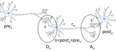
Figure 1: Labels for neurons and synapses in a neural network.

For each synapse $s\in\cal{S}$, $w_{s}$ denotes its strength. For each neuron $n\in\cal{N}$, $p_{n}$ denotes its membrane potential and $r_{n}$ denotes its firing rate, which is the output of the neuron.

In a neuron $n\in\cal{N}$, signals are transmitted from $D_{n}$ to $A_{n}$ in the following order. (1) Postsynaptic potentials are generated following activation of a synapse by neurotransmitters. (2) Postsynaptic potentials are spatially and temporally integrated at the soma. (3) Action potentials is triggered along the axon hillock and propagated along the axon. (4) Neurotransmitters is released from presynaptic terminals.

In a neuron $n\in\cal{N}$, the firing rate is defined as the reciprocal of the interspike interval. The synapse strength $w_{s}$ of a synapse is proportional to the quantity of neurotransmitters released when a spike arrives at the synapse. We assume that the short-time average of the postsynaptic potential is proportional to the product of the synapse strength $w_{s}$ and the presynaptic firing rate $r_{pre_{s}}$. The membrane potential $p_{n}$ is the sum of the postsynaptic potentials as follows.

$$p_{n}=\sum_{s\in D_{n}}\epsilon_{s}\eta_{s}w_{s}r_{pre_{s}}-\theta_{n},$$ (1)

where $\eta_{s}$ is the decremental conduction coefficient of $s$ [34]; and $\theta_{n}$ is the offset of the membrane potential of $n$ [35].

The firing rate $r_{n}$ is a sigmoidal function of its membrane potential as follows.

$$r_{n}=\rho_{n}\sigma(\lambda_{n}p_{n}),$$ (2)

where $\rho_{n}$ is the maximal firing rate of $n$; and $\lambda_{n}$ is the measure of the steepness of the sigmoidal characteristic of $n$.

III The B-L Learning Algorithm

Different learning algorithms have been proposed in the literature to learn the strengths of synapses so that some error is minimized. The following least square error is widely used for learning.

$$\begin{split}E=\frac{1}{2}\sum_{n\in{\cal{O}}}(r_{n}-\bar{r}_{n})^{2},\end{split}$$ (3)

where ${\cal{O}}$ is the set of output neurons and $\bar{r}_{n}$ is the desired/target output of an output neuron.

Among different learning algorithms, the B-P algorithm is very popular. On the other hand, the B-L algorithm is mathematically equivalent to the B-P algorithm and is give by

$$\begin{split}\dot{w_{s}}=&\alpha_{s}\epsilon_{s}r_{pre_{s}}\rho_{post_{s}}\lambda_{post_{s}}\sigma^{\prime}(\lambda_{post_{s}}p_{post_{s}})\\ &(\frac{1}{r_{post_{s}}}\sum_{s^{\prime}\in A_{post_{s}}}\frac{\eta_{s^{\prime}}}{\alpha_{s^{\prime}}}w_{s^{\prime}}\dot{w}_{s^{\prime}}-\gamma(r_{post_{s}}-\bar{r}_{post_{s}})).\end{split}$$ (4)

This algorithm reduces the error $E$ monotonically because the following equation is satisfied [1, 2].

$$\dot{w_{s}}=-\alpha_{s}\frac{\gamma}{\eta_{s}}\frac{dE}{dw_{s}}.$$ (5)

It is shown in [1, 2] that the B-L algorithm has the following properties.

1. The B-L algorithm and the B-P algorithm are mathematically equivalent. Hence, they have the same performance and can be used in same applications.

2. The B-L algorithm is easy to implement because it does not require a feedback network for error back-propagation. A feedback-network-free implementation is given in [2].

3. Since it is unlikely that the requirement of feedback network can be met in biological neural networks, removal of feedback network makes the learning according to the B-L algorithm is much more plausible in biological neural networks.

4. In the B-L algorithm, the information needed for dendritic synapses to learn is implicit in the weights and their derivatives of axonic synapses of the same neuron.

5. The B-L algorithm allows a phaseless learning by processing information asynchronously and concurrently without the needs of a feed-forward phase and a feedback phase.

6. In a layered neural network, all layers will have the same or similar structures using the B-L algorithm. Hence, the B-L algorithm can be implemented in Simulink and other implementation platforms using same or similar blocks.

7. The B-L algorithm provides a much simpler implementation on silicon without complex wiring among neurons, as there is no need to build a separate feedback network and connect it to the feed-forward network.

8. An adaptive neuron can be designed using the B-L algorithm as an identical and standard unit. These adaptive neurons can then be interconnected arbitrarily. This provides the potential for designing neural networks with dynamically reconfigurable topologies.

9. The B-L algorithm are more fault-tolerant since all feedback and connections are local. Hence, failures of some neurons will not significantly affect the entire neural network.

IV Existence of the Solution to the B-L Learning Algorithm

A neural network is called hierarchical if there exists a partial order $\leq$ on ${\cal{N}}$ such that, for $n_{1},n_{2}\in{\cal{N}}$, if $n_{1}\leq n_{2}$, then there exist no axonic synapses of $n_{2}$ with $n_{1}$, that is, $D_{n_{1}}\cap A_{n_{2}}=\emptyset$. This partial order ensures that the output of any neuron $n$ is an explicit function of the outputs of some preceding neurons $n^{\prime}$ satisfying $n^{\prime}\leq n\wedge n^{\prime}\not=n$. Hence, the output of each neuron is always well-defined and unique. Layered neural networks are special cases of hierarchical neural networks.

It is shown in [1, 2] that the B-L algorithm can be used for both hierarchical and non-hierarchical networks. If the network is non-hierarchical, Equation (4) gives only implicit functions of $\dot{w_{s}}$.

To ensure the existence of these implicit functions, let us write Equation (4) in the following matrix form.

$$\left[\begin{array}[]{l}\dot{w_{1}}\\ \dot{w_{2}}\\ ...\\ \dot{w_{S}}\end{array}\right]=\left[\begin{array}[]{llll}g_{11}&g_{12}&...&g_{1S}\\ g_{21}&g_{22}&...&g_{2S}\\ ...\\ g_{S1}&g_{S2}&...&g_{SS}\end{array}\right]\left[\begin{array}[]{l}\dot{w_{1}}\\ \dot{w_{2}}\\ ...\\ \dot{w_{S}}\end{array}\right]+\left[\begin{array}[]{l}h_{1}\\ h_{2}\\ ...\\ h_{S}\end{array}\right]$$

Denote the above matrix equation as

$$\dot{w}=G\dot{w}+h,$$ (6)

where $\dot{w}$ and $h$ are column vectors of $S$ dimension, and $G=[g_{ij}]$ is an $S\times S$ matrix with

$$g_{ij}=\alpha_{i}\epsilon_{i}r_{pre_{i}}\rho_{post_{i}}\lambda_{post_{i}}\sigma^{\prime}(\lambda_{post_{i}}p_{post_{i}})\frac{\eta_{j}w_{j}}{r_{post_{i}}\alpha_{j}},$$

if $j\in A_{post_{i}}$ and $g_{ij}=0$, otherwise.

For the implicit functions of $\dot{w}$ to exist, it is necessary and sufficient that the determinant

$$|I-G|\not=0,$$

where $I$ is the identity matrix of the dimension $S\times S$.

Under this assumption, the solution of $\dot{w}$, denoted by $\dot{w}^{*}$ is given by

$$\dot{w}^{*}=(I-G)^{-1}h.$$

Note that for hierarchical neural networks, the condition of $|I-G|\not=0$ is always satisfied. To prove this, let us enumerate the synapses according to the enumeration of neurons such that

$$j\leq i\Rightarrow post_{j}\leq post_{i}.$$

One such enumeration is to enumerate all synapses in $D_{1}$, then all synapses in $D_{2}$, …, etc. Under such an enumeration, we have

$$j\leq i$$

$$\Rightarrow post_{j}\leq post_{i}$$

$$\Rightarrow D_{post_{j}}\cap A_{post_{i}}=\emptyset$$

$$(\mbox{by the definition of hierarchical networks})$$

$$\Rightarrow j\not\in A_{post_{i}}$$

$$(\mbox{because }j\in D_{post_{j}})$$

$$\Rightarrow g_{ij}=0$$

$$(\mbox{by the definition of }g_{ij}).$$

Hence, $G$ is a triangular matrix with all elements on the diagonal equal 0. Therefore, $|I-G|=1\not=0$.

V Convergence of the B-L Learning Algorithm

In the rest of the paper, we assume that, for a given neural network, the solution $\dot{w}^{*}$ exists, that is, $|I-G|\not=0$. We further assume that the neural network is deep or rich enough so that learning can be accomplished, that is, using a gradient descent algorithm, $\lim_{t\rightarrow\infty}r_{n}(t)=\bar{r}_{n}$, for all $n\in{\cal{O}}$. These two assumptions are reasonable, because, without them, learning cannot be achieved by any learning algorithms.

We investigate the convergence of the B-L algorithm, that is, whether $(\exists\bar{w})\lim_{t\rightarrow\infty}w(t)=\bar{w}$, where $\bar{w}$ is a constant column vector representing the final value of $w$. Clearly, $(\exists\bar{w})\lim_{t\rightarrow\infty}w(t)=\bar{w}$ if and only if $\lim_{t\rightarrow\infty}\dot{w}(t)=0$. Therefore, the B-L algorithm converges if and only if $\lim_{t\rightarrow\infty}\dot{w}(t)=0$.

To check whether $\lim_{t\rightarrow\infty}\dot{w}(t)=0$, let $\dot{w}(t)$ be calculated recursively using Equation (6) as follows. Denote the sample of $\dot{w}(t)$ ($h(t)$, respectively) at time $t_{k}=k\Delta$ by $\dot{w}(k)$ ($h(k)$, respectively), where $k=0,1,2,...$ and $\Delta$ is the sampling period. Let

$$\dot{w}(k+1)=G\dot{w}(k)+h(k).$$

Then,

$$\lim_{t\rightarrow\infty}\dot{w}(t)=0$$

$$\Leftrightarrow \lim_{k\rightarrow\infty}\dot{w}(k)=0$$

$$\Leftrightarrow (\forall\alpha\in eig(G))\ |\alpha|<1\wedge\lim_{k\rightarrow\infty}h(k)=0,$$

where $eig(G)$ denotes the set of eigenvalues of $G$.

Since $\lim_{t\rightarrow\infty}r_{n}(t)=\bar{r}_{n}$, for all $n\in{\cal{O}}$ by assumption, $\lim_{k\rightarrow\infty}h(k)=0$ is true. Therefore, $\lim_{t\rightarrow\infty}\dot{w}(t)=0$ if and only if $(\forall\alpha\in eig(G))\ |\alpha|<1.$

We summarize the above results in the following theorem.

Theorem 1

The B-L algorithm converges if and only if

$$(\forall\alpha\in eig(G))\ |\alpha|<1.\\$$ (7)

We use the maximum of the absolute values of all eigenvalues of $G$ as the measurement of convergence, that is, the convergence measure is given by

$$CM=\max_{\alpha\in eig(G)}\ |\alpha|.$$

Hence, the smaller $CM$ is, the faster the B-L Algorithm converges.

VI Simulation Study

Using Theorem 1 and the convergence measure $CM$ defined above, we can investigate convergence of the B-L algorithm under different parameters by “simulating” the convergence measure $CM$ for those parameters. In the simulations below, we consider the following parameters.

$N$ = the number of neurons.

$B$ = the connection distance, that is, neuron $n$ may be connected to neurons $n^{\prime}\in\{n-B,n-B+1,...,n,n+1,...,n+B\}$.

$C$ = the connection density, that is, the percentage of possible connections that are actually connected.

$D$ = the percentage of synapses that are excitatory ($\epsilon=1$). Hence, $D/(1-D)$ is the ratio of excitatory/inhibitory synapses.

$\hat{p}_{n}$ = the normalized membrane potential, which includes $\lambda$.

$\hat{w}_{s}$ = the normalized synapse strengths, which includes $\rho$ and $\eta$.

For each set of parameters, we run $R=20$ trials, each trial randomly generates a neural network with random connections and with the parameters $\hat{p}_{n}$ and $\hat{w}_{s}$ perturbed by 0%-10% to ensure the robustness of the results. We then take the maximum of $CM$ over $R$ trials as the $CM$ for this set of parameters.

Since the objective of the simulations is to investigate the impacts of different parameters on the convergence of the B-L algorithm, the relative values (rather than the absolute values) of the parameters are of importance. Hence, we start with the following set of parameters

$$\begin{array}[]{lllllll}N=30,&B=20,&C=0.5,\\ D=0.5,&\hat{p}_{n}=5,&\hat{w}_{s}=25.\end{array}$$ (10)

that gives a reasonable $CM\approx 0.8$. In the simulations, we are not concerned with the absolute values $p_{n}$ and $w_{s}$ or their units. We investigate the impact of each parameter on the convergence of the B-L algorithm as described below. The impact of several parameters on the convergence of the B-L algorithm is the sum of the impacts of the parameters involved.

VI-A Convergence vs the number of neurons

To investigate the convergence of the B-L algorithm vs the number of neurons, we simulate neural networks with the number of neurons ranges from 5 to 50 (note that the nominal value is 30). All other parameters are at their nominal values given above. The results are shown in Figure 2.

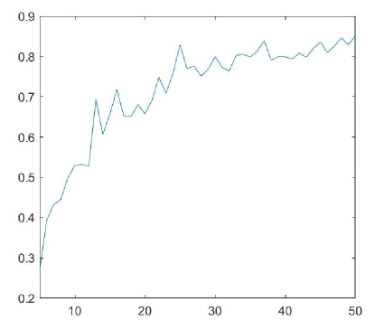
Figure 2: Convergence measure $CM$ (vertical axis) of the B-L algorithm vs number of neurons $N$ (horizontal axis)

The simulations show that the convergence measure increases as the number of neurons increases. In other words, the B-L algorithm converges faster in small neural networks than in large neural networks. On the other hand, the rate of increase in the the convergence measure reduces as the number of neurons increases. The B-L algorithm still converges when $N=50$.

VI-B Convergence vs the connection distance

To investigate the convergence of the B-L algorithm vs the connection distance, we simulate neural networks with the connection distance ranges from 1 to 30 (the maximum). All other parameters are at their nominal values given above. The results are shown in Figure 3.

Figure 3: Convergence measure $CM$ (vertical axis) of the B-L algorithm vs connection distance $B$ (horizontal axis)

The simulations show that the convergence measure increases as the connection distance increases and the increase is less than the linear increase. Hence, the B-L algorithm converges faster in neural networks with local connections than in neural networks with long-distance connections.

VI-C Convergence vs the connection density

To investigate the convergence of the B-L algorithm vs the connection density, we simulate neural networks with the connection density ranges from 0.1 to 0.9. All other parameters are at their nominal values given above. The results are shown in Figure 4.

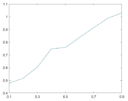
Figure 4: Convergence measure $CM$ (vertical axis) of the B-L algorithm vs connection density $C$ (horizontal axis)

Figure 5: Convergence of the B-L algorithm vs connection density.

The simulations show that the convergence measure increases almost linearly as the connection density increases. Therefore, the B-L algorithm converges slower in neural networks with more dense connections.

VI-D Convergence vs the ratio of excitatory/inhibitory synapses

To investigate the convergence of the B-L algorithm vs the ratio of excitatory/inhibitory synapses, we simulate neural networks with the percentage of synapses that are excitatory ranges from 0.1 to 0.9. All other parameters are at their nominal values given above. The results are shown in Figure 5.

Figure 6: Convergence measure $CM$ (vertical axis) of the B-L algorithm vs percentage of synapses that are excitatory $D$ (horizontal axis)

The simulations show that the convergence measure is smallest when the percentage of synapses that are excitatory is 0.5, that is, when the ratio of excitatory/inhibitory synapses is 1.

Biological neural networks have both excitatory and inhibitory synapses, which is good for the convergence of the B-L algorithm. Having only excitatory synapses or only inhibitory synapses may cause the B-L algorithm not converge.

VI-E Convergence vs the membrane potentials

To investigate the convergence of the B-L algorithm vs the membrane potentials, we simulate neural networks with membrane potential ranges from 4 to 10. All other parameters are at their nominal values given above. The results are shown in Figure 6.

Figure 7: Convergence measure $CM$ (vertical axis) of the B-L algorithm vs membrane potential $\hat{p}_{n}$ (horizontal axis)

The simulations show that the convergence measure decreases almost exponentially as the membrane potentials increases. Therefore, the B-L algorithm converges faster in neural networks with high membrane potentials. Hence, it is important to maintain membrane potentials at certain level in biological neural networks.

VI-F Convergence vs the synapse strengths

To investigate the convergence of the B-L algorithm vs the synapse strengths, we simulate neural networks with the synapse strengths ranges from 20 to 30. All other parameters are at their nominal values given above. The results are shown in Figure 7.

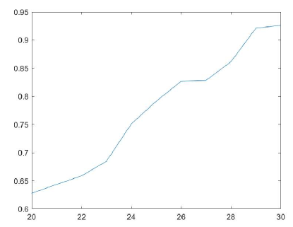
Figure 8: Convergence measure $CM$ (vertical axis) of the B-L algorithm vs synapse strengths $\hat{w}_{s}$ (horizontal axis)

The simulations show that the convergence measure increases as the synapse strengths increases more or less linearly. In other words, the B-L algorithm converges slower in neural networks with large synapse strengths. It is possible that some mechanisms exist in biological neural networks to ensure synapse strengths are not too large.

VII Conclusions

We investigate the convergence of the B-L algorithm in this paper. We first derive a necessary and sufficient condition for the B-L algorithm to converge. We then propose a convergence measure to study the convergence rate of the B-L algorithm. Using simulations, we show how the convergence measure is related to various parameters of neural networks. The parameters include (1) the number of neurons, (2) the connection distance, (3) the connection density, (4) the ratio of excitatory/inhibitory synapses, (5) the membrane potentials, and (6) the synapse strengths. The simulations shows that the membrane potentials have the biggest impact on the convergence of the B-L algorithm.

References

- [1] R. D. Brandt and F. Lin, “Supervised learning in neural networks without feedback network,” in Intelligent Control, 1996., Proceedings of the 1996 IEEE International Symposium on, pp. 86–90, IEEE, 1996.
- [2] F. Lin, “Supervised learning in neural networks: Feedback-network-free implementation and biological plausibility,” IEEE Transactions on Neural Networks and Learning Systems, 2021.
- [3] N. Rochester, J. Holland, L. Haibt, and W. Duda, “Tests on a cell assembly theory of the action of the brain, using a large digital computer,” IRE Transactions on information Theory, vol. 2, no. 3, pp. 80–93, 1956.
- [4] F. Rosenblatt, “The perceptron: a probabilistic model for information storage and organization in the brain.,” Psychological review, vol. 65, no. 6, p. 386, 1958.
- [5] J. J. Hopfield, “Neural networks and physical systems with emergent collective computational abilities,” Proceedings of the national academy of sciences, vol. 79, no. 8, pp. 2554–2558, 1982.
- [6] J. L. McClelland, D. E. Rumelhart, P. R. Group, et al., “Parallel distributed processing,” Explorations in the Microstructure of Cognition, vol. 2, pp. 216–271, 1986.
- [7] Y. Bengio, A. Courville, and P. Vincent, “Representation learning: A review and new perspectives,” IEEE transactions on pattern analysis and machine intelligence, vol. 35, no. 8, pp. 1798–1828, 2013.
- [8] J. Schmidhuber, “Deep learning in neural networks: An overview,” Neural networks, vol. 61, pp. 85–117, 2015.
- [9] Y. LeCun, Y. Bengio, and G. Hinton, “Deep learning,” nature, vol. 521, no. 7553, pp. 436–444, 2015.
- [10] A. Krizhevsky, I. Sutskever, and G. E. Hinton, “Imagenet classification with deep convolutional neural networks,” Communications of the ACM, vol. 60, no. 6, pp. 84–90, 2017.
- [11] C. Ding and D. Tao, “Robust face recognition via multimodal deep face representation,” IEEE Transactions on Multimedia, vol. 17, no. 11, pp. 2049–2058, 2015.
- [12] I. Masi, Y. Wu, T. Hassner, and P. Natarajan, “Deep face recognition: A survey,” in 2018 31st SIBGRAPI conference on graphics, patterns and images (SIBGRAPI), pp. 471–478, IEEE, 2018.
- [13] G. Guo and N. Zhang, “A survey on deep learning based face recognition,” Computer Vision and Image Understanding, vol. 189, p. 102805, 2019.
- [14] A. Graves, A.-r. Mohamed, and G. Hinton, “Speech recognition with deep recurrent neural networks,” in 2013 IEEE international conference on acoustics, speech and signal processing, pp. 6645–6649, IEEE, 2013.
- [15] L. Deng, G. Hinton, and B. Kingsbury, “New types of deep neural network learning for speech recognition and related applications: An overview,” in 2013 IEEE international conference on acoustics, speech and signal processing, pp. 8599–8603, IEEE, 2013.
- [16] A. Hannun, C. Case, J. Casper, B. Catanzaro, G. Diamos, E. Elsen, R. Prenger, S. Satheesh, S. Sengupta, A. Coates, et al., “Deep speech: Scaling up end-to-end speech recognition,” arXiv preprint arXiv:1412.5567, 2014.
- [17] A. B. Nassif, I. Shahin, I. Attili, M. Azzeh, and K. Shaalan, “Speech recognition using deep neural networks: A systematic review,” IEEE Access, vol. 7, pp. 19143–19165, 2019.
- [18] C. Szegedy, A. Toshev, and D. Erhan, “Deep neural networks for object detection,” Advances in neural information processing systems, vol. 26, pp. 2553–2561, 2013.
- [19] D. Erhan, C. Szegedy, A. Toshev, and D. Anguelov, “Scalable object detection using deep neural networks,” in Proceedings of the IEEE conference on computer vision and pattern recognition, pp. 2147–2154, 2014.
- [20] A. R. Pathak, M. Pandey, and S. Rautaray, “Application of deep learning for object detection,” Procedia computer science, vol. 132, pp. 1706–1717, 2018.
- [21] Z.-Q. Zhao, P. Zheng, S.-t. Xu, and X. Wu, “Object detection with deep learning: A review,” IEEE transactions on neural networks and learning systems, vol. 30, no. 11, pp. 3212–3232, 2019.
- [22] V. Mnih, K. Kavukcuoglu, D. Silver, A. Graves, I. Antonoglou, D. Wierstra, and M. Riedmiller, “Playing atari with deep reinforcement learning,” arXiv preprint arXiv:1312.5602, 2013.
- [23] E. Gibney, “Google ai algorithm masters ancient game of go,” Nature News, vol. 529, no. 7587, p. 445, 2016.
- [24] D. Silver, A. Huang, C. J. Maddison, A. Guez, L. Sifre, G. Van Den Driessche, J. Schrittwieser, I. Antonoglou, V. Panneershelvam, M. Lanctot, et al., “Mastering the game of go with deep neural networks and tree search,” nature, vol. 529, no. 7587, pp. 484–489, 2016.
- [25] M. Lanctot, V. Zambaldi, A. Gruslys, A. Lazaridou, K. Tuyls, J. Pérolat, D. Silver, and T. Graepel, “A unified game-theoretic approach to multiagent reinforcement learning,” in Advances in neural information processing systems, pp. 4190–4203, 2017.
- [26] I. Stephen, “Perceptron-based learning algorithms,” IEEE Transactions on neural networks, vol. 50, no. 2, p. 179, 1990.
- [27] R. Caruana and A. Niculescu-Mizil, “An empirical comparison of supervised learning algorithms,” in Proceedings of the 23rd international conference on Machine learning, pp. 161–168, 2006.
- [28] T. O. Ayodele, “Types of machine learning algorithms,” New advances in machine learning, vol. 3, pp. 19–48, 2010.
- [29] N. Japkowicz and M. Shah, Evaluating learning algorithms: a classification perspective. Cambridge University Press, 2011.
- [30] D. E. Rumelhart, G. E. Hinton, and R. J. Williams, “Learning representations by back-propagating errors,” nature, vol. 323, no. 6088, pp. 533–536, 1986.
- [31] F. J. Pineda, “Generalization of back-propagation to recurrent neural networks,” Physical review letters, vol. 59, no. 19, p. 2229, 1987.
- [32] R. Hecht-Nielsen, “Theory of the backpropagation neural network,” in Neural networks for perception, pp. 65–93, Elsevier, 1992.
- [33] Y. Chauvin and D. E. Rumelhart, Backpropagation: theory, architectures, and applications. Psychology Press, 2013.
- [34] R. L. De Nó and G. Condouris, “Decremental conduction in peripheral nerve. integration of stimuli in the neuron,” Proceedings of the National Academy of Sciences of the United States of America, vol. 45, no. 4, p. 592, 1959.
- [35] K. Montaigne and W. F. Pickard, “Offset of the vacuolar potential of characean cells in response to electromagnetic radiation over the range 250 hz-250 khz,” Bioelectromagnetics: Journal of the Bioelectromagnetics Society, The Society for Physical Regulation in Biology and Medicine, The European Bioelectromagnetics Association, vol. 5, no. 1, pp. 31–38, 1984.