Testing Symmetry for Bivariate Copulas using Bernstein Polynomials

Abstract

In this work, tests of symmetry for bivariate copulas are introduced and studied using empirical Bernstein copula process. Three statistics are proposed and their asymptotic properties are established. Besides, a multiplier bootstrap Bernstein version is investigated for implementation purpose. The simulation study demonstrated the superior performance of the Bernstein tests compared to tests based on empirical copulas. Furthermore, in real data applications, these tests consistently yielded similar conclusions across a diverse range of scenarios.

  Keywords: Empirical Bernstein process; Multiplier bootstrap; Empirical copula process; Symmetry.

 

1 Introduction

Asymmetric copulas have massive explorations and applications in recent years. They are powerful tools for capturing the asymmetrical dependence structure and have been applied in many fields, for instance, Grimaldi and Serinaldi (2006) for flood frequency analysis, Wu (2014) in reliability modelling and Zhang et al. (2018) for ocean data analysis. Meanwhile, more attention is given to testing and identifying the symmetric nature of a copula. Genest et al. (2012) proposed tests based on empirical copula, Bahraoui et al. (2018) used empirical copula characteristic function to construct the test,  Jaser and Min (2021) developed a test by representing copula as a mixture of two conditional distribution functions, Beare and Seo (2020) studied a randomization procedure. For $d$-variate symmetry tests, the work of Genest et al. (2012) was extended by Harder and Stadtmüller (2017), and Bahraoui and Quessy (2022) investigated tests based on Lévy measures.

In this work, tests of symmetry for bivariate copulas based on empirical Bernstein copula process are proposed. Specifically, consider a random pair $(X,Y)$ with cumulative distribution function $F_{XY}(x,y)=\mathbb{P}(X\leq x,Y\leq y)$ and continuous margins $F_{X}$ and $F_{Y}$. According to Sklar (1959), there exists a unique copula function $C$ such that

$$F_{XY}(x,y)=C\{F_{X}(x),F_{Y}(y)\}.$$

To detect the symmetry of copula $C$, one would like to test the following hypotheses

$${}\begin{cases}\mathscr{H}_{0}\mathrel{\mathop{\ordinarycolon}}\forall(u,v)\in[0,1]^{2}&C(u,v)=C(v,u),\\ &\text{versus}\\ \mathscr{H}_{1}\mathrel{\mathop{\ordinarycolon}}\exists(u,v)\in[0,1]^{2}&C(u,v)\neq C(v,u).\end{cases}$$ (1)

The symmetry property of bivariate copulas has intimate relation with the symmetry of corresponding random pairs and was discussed in Nelsen (1993, 2006) and Nelson (2007). It was shown that $X$ and $Y$ are exchangeable, $i.e.$, $F_{XY}(x,y)=F_{XY}(y,x)$ if and only if $F_{X}=F_{Y}$, and $C(u,v)=C(v,u)$ for $(u,v)\in[0,1]^{2}$. Specifically, for identically distributed margins, the symmetry structure of the copula can determine the exchangeability of the random variables $X$ and $Y$. Identifying the equality of margins is well-developed and can be investigated using Kolmogorov-Smirnov test or Cramér-von Mises test. For a positively dependent survival data setting, see Fujii (1989) and for a high-dimensional data setting, see Cousido-Rocha et al. (2019). Together with the verification of equal margins, approaches to detecting the symmetry of the copula function would provide an effective way to decide on the exchangeability of two random variables. As the equality of margins was already discussed vigorously by many others, the contribution of detecting the symmetry of copula becomes more appealing for deciding the exchangeability of two random variables. Moreover, before fitting a specific copula model to the data, identifying the symmetric structure can assist us to choose an appropriate model, for example, Archimedean copulas are symmetric.

Empirical Bernstein copula has drawn attention in recent years due to free boundary bias properties and tractability of implementation. Indeed, one only needs to select the degree of the Bernstein polynomials during deployment. Theoretical properties of this estimator have been well-studied, see Sancetta and Satchell (2004), Janssen et al. (2012), Belalia et al. (2017) and Segers et al. (2017), among others. However, computational investigations of the empirical processes based on this estimator are barely explored. To fill this gap, we proposed a smooth version of multiplier bootstrap method for empirical Bernstein copula process with promising performance.

The rest of this paper is structured as follows. In Section 2, based on the empirical Bernstein copula, an extension of symmetry test statistics in Genest et al. (2012) is proposed and their asymptotic behaviours are examined. Section 3 develops the empirical Bernstein copula process multiplier bootstrap and its large sample behaviour. Simulation studies are carried out in Section 4. Two real data applications are presented in Section 5. Some concluding remarks are given in Section 6. Finally, the proofs are relegated in the Appendix and the R code that was used in this article is available on GitHub.

2 New testing procedures based on empirical Bernstein copula

2.1 Descriptive of the test statistics

Let $(X_{1},Y_{1}),\ldots,(X_{n},Y_{n})$ be a random sample from a bivariate distribution $F_{XY}$ with continuous margins $F_{X}$ and $F_{Y}$. Also, let $C$ be their associated copula. Unfortunately, this function is generally unknown, hence it has to be estimated. The empirical copula introduced by Rüschendorf (1976) is a natural nonparametric estimator of $C$ and is given by

$$\widehat{C}_{n}(u,v)=\frac{1}{n}\sum_{i=1}^{n}{\mathbb{I}}\left(\widehat{U}_{i}\leq u,\widehat{V}_{i}\leq v\right),$$ (2)

where $\widehat{U}_{i}=n^{-1}\sum_{j=1}^{n}{\mathbb{I}}\left(X_{j}\leq X_{i}\right)$ and $\widehat{V}_{i}=n^{-1}\sum_{j=1}^{n}{\mathbb{I}}\left(Y_{j}\leq Y_{i}\right)$ are the empirical distributions of the margins.

The empirical copula is widely used for construction of nonparametric tests in the literature, such as, test of independence, goodness-of-fit test among others. However, it is not a continuous estimator for $C$, which mismatches the continuity of the copula function. To overcome this drawback, smoothed empirical copulas were developed, for example, Morettin et al. (2010) introduced wavelet-smoothed empirical copula for time series data,  Gijbels and Mielniczuk (1990), Fermanian et al. (2004), Chen and Huang (2007), Omelka et al. (2009) considered kernel-smoothed empirical copula and Genest et al. (2017) proposed empirical checkerboard copula. Here, the empirical Bernstein copula is employed. This choice is motivated by (i) estimation based on Bernstein polynomials is known to be asymptotically bias free at boundary points (see, Leblanc (2012), Janssen et al. (2012), Belalia (2016)) as compared to kernel based methods which suffer from excessive bias at or near to the boundary points. A good discussion about the boundary bias for kernel based methods can be found in Chen and Huang (2007). (ii) The empirical Bernstein copula is a polynomial, hence, it has all partial derivatives, which will be of highly important for building our multiplier bootstrap. Besides, the support of bivariate copula is $[0,1]^{2}$ which meets the Bernstein polynomials assumption perfectly.

The empirical Bernstein copula estimator of order $m$ is defined as

$$\widehat{C}_{n,m}(u,v) =\sum_{k=0}^{m}\sum_{\ell=0}^{m}\widehat{C}_{n}\left(k/m,\ell/m\right)P_{m,k}(u)P_{m,\ell}(v)$$

$$=\frac{1}{n}\sum_{i=1}^{n}\sum_{k=0}^{m}\sum_{\ell=0}^{m}{\mathbb{I}}\left(\widehat{U}_{i}\leq k/m,\widehat{V}_{i}\leq\ell/m\right)P_{m,k}(u)P_{m,\ell}(v),$$ (3)

where $P_{m,k}(u)=\binom{m}{k}u^{k}(1-u)^{m-k}$ is the binomial probability mass function. Note that, $m$ is dependent on $n$, in particular, if the degree of Bernstein polynomial $m$ is equal to the sample size $n$, the estimator (2.1) turns out to be the empirical beta copula developed by Segers et al. (2017). Resampling procedures with the empirical beta copula are proposed and studied in Kiriliouk et al. (2021). A broad class of smooth, possibly data-adaptive nonparametric copula estimators are proposed in Kojadinovic and Yi (2021) and Kojadinovic (2022), which includes the empirical Bernstein and beta copula.

In the same spirit as the one presented in Genest et al. (2012), Kolmogorov-Smirnov and Cramér-von Mises type statistics are proposed. Specifically, these statistics are built upon the empirical Bernstein copula and are presented as follows:

$$R_{n,m} =\int_{0}^{1}\int_{0}^{1}\Big{\{}\widehat{C}_{n,m}(u,v)-\widehat{C}_{n,m}(v,u)\Big{\}}^{2}\operatorname{d\!}u\operatorname{d\!}v,$$

$$S_{n,m} =\int_{0}^{1}\int_{0}^{1}\Big{\{}\widehat{C}_{n,m}(u,v)-\widehat{C}_{n,m}(v,u)\Big{\}}^{2}\operatorname{d\!}\widehat{C}_{n}(u,v),$$

$$T_{n,m} =\sup_{(u,v)\in[0,1]^{2}}\left|\widehat{C}_{n,m}(u,v)-\widehat{C}_{n,m}(v,u)\right|.$$ (4)

In what follows, the asymptotic behaviour of the three test statistics will be studied, including the asymptotic limit under both the null and alternative hypotheses.

2.2 Asymptotic behaviour of the test statistics

As it will be seen, the limits of the proposed test statistics are functional of the unknown underlying copula $C$, therefore, some common assumptions are needed before going further.

Assumption 1.

Assume that first-order partial derivatives $\dot{C}_{1}(u,v)=\partial C(u,v)/\partial u,\dot{C}_{2}(u,v)=\partial C(u,v)/\partial v$ exist and are continuous, respectively, on the sets $(0,1)\times[0,1]$ and $[0,1]\times(0,1)$.

Assumption 2.

Assume that second-order partial derivatives $\ddot{C}_{11}(u,v)=\partial^{2}C(u,v)/\partial u^{2},\ddot{C}_{21}(u,v)=\partial^{2}C(u,v)/\partial u\partial v$ and $\ddot{C}_{22}(u,v)=\partial^{2}C(u,v)/\partial v^{2}$ exist and are continuous, respectively, on the sets $(0,1)\times[0,1],(0,1)\times(0,1)$ and $[0,1]\times(0,1)$, and there exists a constant $K>0$ such that

$$\left|\ddot{C}_{11}(u,v)\right|\leq\frac{K}{u(1-u)},\quad\left|\ddot{C}_{21}(u,v)\right|\leq K\min\left(\frac{1}{u(1-u)},\frac{1}{v(1-v)}\right),\quad\left|\ddot{C}_{22}(u,v)\right|\leq\frac{K}{v(1-v)}.$$

Let $\mathbb{B}_{n,m}$ and $\mathbb{S}_{n,m}$ denote, respectively, the empirical Bernstein copula process and symmetrised empirical Bernstein copula process, namely, for all $(u,v)\in[0,1]^{2}$

$$\mathbb{B}_{n,m}(u,v)=\sqrt{n}\Big{\{}\widehat{C}_{n,m}(u,v)-C(u,v)\Big{\}},\quad\mathbb{S}_{n,m}(u,v)=\sqrt{n}\Big{\{}\widehat{C}_{n,m}(u,v)-\widehat{C}_{n,m}(v,u)\Big{\}}.$$

From the work of Segers et al. (2017), suppose $C$ satisfies Assumption 1 and $m=cn^{\alpha}$ with $c>0,\alpha\geqslant 1$, then, in $\ell^{\infty}([0,1]^{2})$ (the Banach space of all real-valued, bounded functions on $[0,1]^{2}$, equipped with sup-norm),

$$\mathbb{B}_{n,m}(u,v)\rightsquigarrow\mathbb{B}_{C}(u,v)=\mathbb{C}(u,v)-\dot{C}_{1}(u,v)\mathbb{C}(u,1)-\dot{C}_{2}(u,v)\mathbb{C}(1,v),\quad\text{as $n\rightarrow\infty$},$$ (5)

where $\mathbb{C}$ is a $C$-Brownian bridge whose covariance function is

$$\Gamma_{\mathbb{C}}(u,v,s,t)=C(\min(u,s),\min(v,t))-C(u,v)C(s,t),$$

for $(u,v),(s,t)\in[0,1]^{2}$ and $``\rightsquigarrow$” stands for the weak convergence. Based on this result, the weak convergence of the symmetrised empirical Bernstein copula process is presented in the following theorem.

Theorem 1.

Let $C$ be a symmetric copula satisfying Assumption 1, in addition, if $m=cn^{\alpha}$ with $c>0,\alpha\geqslant 1$, then as $n\rightarrow\infty$, $\mathbb{S}_{n,m}$ converges weakly to a Gaussian process $\mathbb{S}_{C}$ defined by

$$\mathbb{S}_{C}(u,v)=\mathbb{D}(u,v)-\dot{C}_{1}(u,v)\mathbb{D}(u,1)-\dot{C}_{2}(u,v)\mathbb{D}(1,v),$$

for all $(u,v)\in[0,1]^{2}$, where $\mathbb{D}$ is a $C$-Brownian bridge with covariance function given at each $(u,v),(s,t)\in[0,1]^{2}$ by $\Gamma_{\mathbb{D}}(u,v,s,t)=2\{\Gamma_{\mathbb{C}}(u,v,s,t)-\Gamma_{\mathbb{C}}(u,v,t,s)\}$.

Proof.

Using similar approach as in Genest et al. (2012, Proof of Prosition 2), under the null hypothesis, one can write that,

$$\mathbb{S}_{n,m}(u,v) =\sqrt{n}\left\{\hat{C}_{n,m}(u,v)-\hat{C}_{n,m}(v,u)\right\}-\sqrt{n}C(u,v)+\sqrt{n}C(v,u)$$

$$=\mathbb{B}_{n,m}(u,v)-\mathbb{B}_{n,m}(v,u).$$

Further, it was shown in Segers et al. (2017), that $\mathbb{B}_{n,m}\rightsquigarrow\mathbb{B}_{C}$ as $n\rightarrow\infty$. Then, the desired result can be proven using continuous mapping theorem, namely,

$$\mathbb{S}_{n,m}\rightsquigarrow\mathbb{S}_{C},$$

where $\mathbb{S}_{C}(u,v)=\mathbb{B}_{C}(u,v)-\mathbb{B}_{C}(v,u)$. ∎

Based on Theorem 1 and the fact that the proposed test statistics in (2.1) are functional of $\mathbb{S}_{n,m}$, their asymptotic behaviours under the null hypothesis can be established as follows.

Theorem 2.

Let $C$ be a symmetric copula satisfying Assumption 1, in addition, if $m=cn^{\alpha}$ with $c>0,\alpha\geqslant 1$, then as $n\rightarrow\infty$,

$$nR_{n,m}=\int_{0}^{1}\int_{0}^{1}\big{\{}\mathbb{S}_{n,m}(u,v)\big{\}}^{2}\operatorname{d\!}u\operatorname{d\!}v \rightsquigarrow\mathbb{L}_{R}=\int_{0}^{1}\int_{0}^{1}\big{\{}\mathbb{S}_{C}(u,v)\big{\}}^{2}\operatorname{d\!}u\operatorname{d\!}v,$$

$$nS_{n,m}=\int_{0}^{1}\int_{0}^{1}\big{\{}\mathbb{S}_{n,m}(u,v)\big{\}}^{2}\operatorname{d\!}\widehat{C}_{n}(u,v) \rightsquigarrow\mathbb{L}_{S}=\int_{0}^{1}\int_{0}^{1}\big{\{}\mathbb{S}_{C}(u,v)\big{\}}^{2}\operatorname{d\!}C(u,v),$$

$$n^{1/2}T_{n,m}=\underset{(u,v)\in[0,1]^{2}}{\sup}|\mathbb{S}_{n,m}(u,v)| \rightsquigarrow\mathbb{L}_{T}=\underset{(u,v)\in[0,1]^{2}}{\sup}\left|\mathbb{S}_{C}(u,v)\right|.$$

Proof of Theorem 2.

The proof is postponed to the appendix. ∎

More generally, the asymptotic behaviours of the test statistics under the alternative hypothesis are given as follows.

Theorem 3.

Let $C$ be a copula satisfying Assumption 1, in addition, if $m=cn^{\alpha}$ with $c>0,\alpha\geqslant 1$, then as $n\rightarrow\infty$,

$$R_{n,m} \xrightarrow{a.s.}R_{C}=\int_{0}^{1}\int_{0}^{1}\Big{\{}C(u,v)-C(v,u)\Big{\}}^{2}\operatorname{d\!}u\operatorname{d\!}v,$$

$$S_{n,m} \xrightarrow{a.s.}S_{C}=\int_{0}^{1}\int_{0}^{1}\Big{\{}C(u,v)-C(v,u)\Big{\}}^{2}\operatorname{d\!}C(u,v),$$

$$T_{n,m} \xrightarrow{a.s.}T_{C}=\sup_{(u,v)\in[0,1]^{2}}\left|C(u,v)-C(v,u)\right|.$$

Specifically, under the alternative hypothesis, as $n\to\infty$,

$$nR_{n,m}\xrightarrow{a.s.}\infty,\quad nS_{n,m}\xrightarrow{a.s.}\infty,\quad\sqrt{n}T_{n,m}\xrightarrow{a.s.}\infty,$$

which ensures the consistency of the proposed test statistics.

Proof of Theorem 3.

The proof is postponed to the appendix. ∎

Remark 1.

Note that, the convergence in Theorem 1-3 also hold under Assumption 1-2 with a weaker condition on $m$, that is, $m=cn^{\alpha}$ with $c>0,\alpha>3/4$.

Lemma 1.

Suppose that $C$ satisfies Assumption 1-2, if $m=cn^{\alpha}$ with $c>0,\alpha>3/4$, then, in $\ell^{\infty}([0,1]^{2})$, Equation (5) holds.

Proof of Lemma 1.

The proof is postponed to the appendix. ∎

3 Multiplier bootstrap

As shown in the preceding section, the asymptotic limits of the statistics are functions of the unknown copula $C$, therefore it is impossible to compute valid P-values using standard Monte Carlo procedure directly. To overcome this issue, different bootstrap methods were developed, see for example Genest et al. (2009) and Belalia et al. (2017) among others. However, these approaches are computationally intensive, especially when the sample size is large. The multiplier bootstrap is an alternative methodology that mitigates the burden of computation by estimating the replicates of statistics under null hypothesis straightly. For the application of this method, the reader is directed to Rémillard and Scaillet (2009), Genest et al. (2012),  Bahraoui et al. (2018) and references therein.

Following the multiplier procedure described in Harder and Stadtmüller (2017), let $H\in\mathbb{N}$ and for each $h\in\{1,\ldots,H\}$, let $\bm{\xi}_{n}^{(h)}=\left(\xi_{1}^{(h)},\ldots,\xi_{n}^{(h)}\right)$ be a vector of independent random variables with unit mean and unit variance (taking $\xi_{i}^{(h)}\sim\rm{Exp}(1)$, $i=1,\ldots,n$). Set

$$C_{n,m}(u,v)=\frac{1}{n}\sum_{i=1}^{n}\sum_{k=0}^{m}\sum_{\ell=0}^{m}{\mathbb{I}}\left(U_{i}\leq\frac{k}{m},V_{i}\leq\frac{\ell}{m}\right)P_{m,k}(u)P_{m,\ell}(v),$$

where $\left(U_{i},V_{i}\right)=\left(F_{X}\left(X_{i}\right),F_{Y}\left(Y_{i}\right)\right)$. Denote the sample mean of $\bm{\xi}_{n}^{(h)}$ by $\bar{\xi}_{n}^{(h)}$, then for each $h$, define

$$\widetilde{\mathbb{B}}_{n,m}(u,v) =n^{1/2}\big{\{}C_{n,m}(u,v)-C(u,v)\big{\}}$$

$$=n^{1/2}\Bigg{\{}\frac{1}{n}\sum_{i=1}^{n}\sum_{k=0}^{m}\sum_{\ell=0}^{m}\bigg{\{}{\mathbb{I}}\left(U_{i}\leq\frac{k}{m},V_{i}\leq\frac{\ell}{m}\right)-C(u,v)\bigg{\}}P_{m,k}(u)P_{m,\ell}(v)\Bigg{\}},$$

and

$$\overline{\mathbb{B}}_{n,m}^{(h)}(u,v) =n^{1/2}\Bigg{\{}\frac{1}{n}\sum_{i=1}^{n}\sum_{k=0}^{m}\sum_{\ell=0}^{m}\left(\xi^{(h)}_{i}-\bar{\xi}_{n}^{(h)}\right){\mathbb{I}}\left(\widehat{U}_{i}\leq\frac{k}{m},\widehat{V}_{i}\leq\frac{\ell}{m}\right)P_{m,k}(u)P_{m,\ell}(v)\Bigg{\}}.$$ (6)

One can observe that $\widetilde{\mathbb{B}}_{n,m}$ is the empirical Bernstein copula process when margins are known. The following proposition states that $\widetilde{\mathbb{B}}_{n,m}$ converges weakly to the $C$-Brownian bridge $\mathbb{C}$ mentioned in (5), moreover, $\overline{\mathbb{B}}_{n,m}^{(h)}$ is a valid replicate of $\widetilde{\mathbb{B}}_{n,m}$.

Proposition 1.

Let $C$ be a symmetric copula satisfying Assumption 1-2, if $m=cn^{\alpha}$ with $c>0,\alpha>3/4$, then for $(u,v)\in[0,1]^{2}$,

1. we have

   $$\widetilde{\mathbb{B}}_{n,m}(u,v)\rightsquigarrow\mathbb{C}(u,v),$$

2. also, for each $h\in\{1,\ldots,H\}$,

   $$\overline{\mathbb{B}}_{n,m}^{(h)}(u,v)\rightsquigarrow\mathbb{C}(u,v).$$ (7)

Proof of Proposition 1.

The proof is postponed to the appendix. ∎

Hence the bootstrap replicates of $\mathbb{B}_{n,m}(u,v)$ for $h\in\{1,\ldots,H\}$ are

$$\mathbb{B}_{n,m}^{(h)}(u,v)=\overline{\mathbb{B}}^{(h)}_{n,m}(u,v)-\frac{\partial\widehat{C}_{n,m}(u,v)}{\partial u}\overline{\mathbb{B}}^{(h)}_{n,m}(u,1)-\frac{\partial\widehat{C}_{n,m}(u,v)}{\partial v}\overline{\mathbb{B}}^{(h)}_{n,m}(1,v).$$ (8)

The partial derivatives of the empirical Bernstein copula were studied in Janssen et al. (2016), more specifically,

$$\frac{\partial\widehat{C}_{n,m}(u,v)}{\partial u} =m\sum_{k=0}^{m-1}\sum_{\ell=0}^{m}\bigg{\{}\widehat{C}_{n}\left(\frac{k+1}{m},\frac{\ell}{m}\right)-\widehat{C}_{n}\left(\frac{k}{m},\frac{\ell}{m}\right)\bigg{\}}P_{m-1,k}(u)P_{m,\ell}(v),$$

$$\frac{\partial\widehat{C}_{n,m}(u,v)}{\partial v} =m\sum_{k=0}^{m}\sum_{\ell=0}^{m-1}\bigg{\{}\widehat{C}_{n}\left(\frac{k}{m},\frac{\ell+1}{m}\right)-\widehat{C}_{n}\left(\frac{k}{m},\frac{\ell}{m}\right)\bigg{\}}P_{m,k}(u)P_{m-1,\ell}(v).$$

Unlike the empirical copula, the partial derivatives of the empirical Bernstein copula can be calculated directly without any further approximations. The following proposition provides the uniform consistency of partial derivatives.

Proposition 2.

Let $C$ be a copula satisfying Assumption 1-2, if $m=cn^{\alpha}$ with $c>0,\alpha>3/4$ and $b_{n}=\kappa n^{-\beta}$ with $\kappa>0,\beta<{\alpha}/{2}$, then

$$\sup_{\begin{subarray}{c}v\in[0,1],\\ u\in[b_{n},1-b_{n}]\end{subarray}}\left|\frac{\partial\widehat{C}_{n,m}(u,v)}{\partial u}-\dot{C}_{1}(u,v)\right| =O\left(m^{1/2}n^{-1/2}(\log\log n)^{1/2}\right),$$

$$\sup_{\begin{subarray}{c}u\in[0,1],\\ v\in[b_{n},1-b_{n}]\end{subarray}}\left|\frac{\partial\widehat{C}_{n,m}(u,v)}{\partial v}-\dot{C}_{2}(u,v)\right| =O\left(m^{1/2}n^{-1/2}(\log\log n)^{1/2}\right),$$

almost surely as $n\to\infty$.

Proof of Proposition 2.

The proof is postponed to the appendix. ∎

The limiting behaviour of the multiplier replicates of the symmetrised empirical copula process are stated in the following theorem.

Theorem 4.

Let $C$ be a symmetric copula satisfying Assumption 1-2, if $m=cn^{\alpha}$ with $3/4<\alpha<1$ and $c>0$ , then for $(u,v)\in(0,1)^{2}$,

$$\left(\mathbb{S}_{n,m},\mathbb{S}_{n,m}^{(1)},\ldots,\mathbb{S}_{n,m}^{(H)}\right)\rightsquigarrow\left(\mathbb{S}_{C},\mathbb{S}_{C}^{(1)},\ldots,\mathbb{S}_{C}^{(H)}\right),$$

as $n\rightarrow\infty$, where for each $h\in\{1,\ldots,H\}$,

$$\mathbb{S}_{n,m}^{(h)}(u,v) =\mathbb{B}_{n,m}^{(h)}(u,v)-\mathbb{B}_{n,m}^{(h)}(v,u)$$

$$=\overline{\mathbb{S}}^{(h)}_{n,m}(u,v)+\frac{\partial\widehat{C}_{n,m}(u,v)}{\partial u}\overline{\mathbb{S}}^{(h)}_{n,m}(u,1)-\frac{\partial\widehat{C}_{n,m}(u,v)}{\partial v}\overline{\mathbb{S}}^{(h)}_{n,m}(1,v),$$

and $\overline{\mathbb{S}}^{(h)}_{n,m}(u,v)=\overline{\mathbb{B}}^{(h)}_{n,m}(u,v)-\overline{\mathbb{B}}^{(h)}_{n,m}(v,u)$.

Proof of Theorem 4.

Given that under the null hypothesis

$$\dot{C}_{1}(u,v)=\dot{C}_{2}(v,u),$$

the proof is a direct application of Proposition 2 and the continuous mapping theorem. ∎

Combining Theorems 2 and 4, the asymptotic properties of replicates of statistics defined by (2.1) are established in the following corollary.

Corollary 1.

Let $C$ be a symmetric copula satisfying Assumption 1-2, if $m=cn^{\alpha}$ with $3/4<\alpha<1$ and $c>0$, then as $n\rightarrow\infty$, for all $H\in{\mathbb{N}}$, one has

$$\left(nR_{n,m},nR_{n,m}^{(1)},\ldots,nR_{n,m}^{(H)}\right) \rightsquigarrow\left(\mathbb{L}_{R},\mathbb{L}_{R}^{(1)},\ldots,\mathbb{L}_{R}^{(H)}\right),$$

$$\left(nS_{n,m},nS_{n,m}^{(1)},\ldots,nS_{n,m}^{(H)}\right) \rightsquigarrow\left(\mathbb{L}_{S},\mathbb{L}_{S}^{(1)},\ldots,\mathbb{L}_{S}^{(H)}\right),$$

$$\left(n^{1/2}T_{n,m},n^{1/2}T_{n,m}^{(1)},\ldots,n^{1/2}T_{n,m}^{(H)}\right) \rightsquigarrow\left(\mathbb{L}_{T},\mathbb{L}_{T}^{(1)},\ldots,\mathbb{L}_{T}^{(H)}\right).$$

Remark 2.

Note that, under Assumption 1-2, the proposed statistics together with multiplier bootstraps can be valid under the same magnitude requirement of $m$, which is $m=cn^{\alpha}$ with $c>0,3/4<\alpha<1$.

It follows directly from Corollary 1 that P-values of the proposed tests can be computed as

$$\frac{1}{H}\sum_{h=1}^{H}{\mathbb{I}}\left(R_{n,m}^{(h)}\geqslant R_{n,m}\right),\quad\frac{1}{H}\sum_{h=1}^{H}{\mathbb{I}}\left(S_{n,m}^{(h)}\geqslant S_{n,m}\right),\quad\frac{1}{H}\sum_{h=1}^{H}{\mathbb{I}}\left(T_{n,m}^{(h)}\geqslant T_{n,m}\right).$$

This approach will be employed to obtain the empirical level and power as shown in the next section.

4 Finite sample performance

The finite sample performance of the proposed testing procedure is investigated in this section through a Monte Carlo experiment. All the tests were conducted with $500$ repetitions under $5\%$ nominal level using $H=200$ multiplier replicates, also since the statistics shown in Theorem 2 involve integration, a discrete approximation is applied with size of integration grid $N=20$ (i.e. $20\times 20$ points on $[0,1]^{2}$).

4.1 Comparison with the empirical copula-based tests

To assess the improvement of the empirical Bernstein copula process-based tests defined in (7) and denoted by $\{R_{n,m},S_{n,m},T_{n,m}\}$, the empirical level and power of the proposed tests were compared with the tests based on the empirical copula process in Genest et al. (2012) denoted by $\{R_{n},S_{n},T_{n}\}$. For the empirical size, samples with sizes $n=\{50,100,200\}$ were generated from the Gaussian, Clayton, Gumbel-Hougaard and Frank copulas with Kendall’s tau $\tau=0.25$. Since the Bernstein order $m$ is dependent on the sample size, $m$ is chosen using $m=\lfloor cn^{\alpha}\rfloor=\{9,13,15\}$, where $\alpha=4/5$ and $c=\{0.40,0.33,0.22\}$.

The empirical level of the tests are presented in Table 1. Evidently, a significant portion of the Bernstein tests falls below their designated nominal level; however, their performance surpasses that of the empirical tests.

Table 1: Level ($\%$) of the tests of $\mathscr{H}_{0}$ based on $\{R_{n},S_{n},T_{n}\}$ and $\{R_{n,m},S_{n,m},T_{n,m}\}$, as estimated from $500$ samples from symmetric copulas using $H=200$ multiplier bootstrap replicates with Bernstein order $m=\{9,13,15\}$ associated with sample size $n=\{50,100,200\}$.

Model	$(n,m)$	$R_{n}$	$R_{n,m}$	$S_{n}$	$S_{n,m}$	$T_{n}$	$T_{n,m}$
$\rm{Gaussian}$	$(50,9)$	$1.2$	$2.0$	$3.2$	$3.4$	$1.0$	$2.0$
	$(100,13)$	$2.6$	$4.6$	$4.4$	$5.2$	$2.8$	$4.0$
	$(200,15)$	$2.8$	$3.4$	$1.8$	$3.6$	$7.4$	$3.8$
$\rm{Clayton}$	$(50,9)$	$1.2$	$3.2$	$4.2$	$4.2$	$1.0$	$2.2$
	$(100,13)$	$1.0$	$3.6$	$3.6$	$3.8$	$1.8$	$2.6$
	$(200,15)$	$4.4$	$4.6$	$4.2$	$5.2$	$6.2$	$4.2$
$\rm{Gumbel}$	$(50,9)$	$0.8$	$3.2$	$3.4$	$3.8$	$0.4$	$1.6$
$\rm{Hougaard}$	$(100,13)$	$1.8$	$4.0$	$2.8$	$3.4$	$1.8$	$2.8$
	$(200,15)$	$3.0$	$4.2$	$2.6$	$4.0$	$6.2$	$4.0$
$\rm{Frank}$	$(50,9)$	$1.4$	$2.4$	$3.4$	$3.4$	$1.6$	$2.2$
	$(100,13)$	$2.6$	$2.6$	$2.2$	$2.6$	$1.6$	$2.8$
	$(200,15)$	$3.6$	$3.8$	$4.0$	$4.4$	$6.4$	$4.0$

To study the power of the considered tests, samples of sizes $n=100$ and $n=200$ were generated from the Gaussian (GA), Frank (FR), Gumbel-Hougaard (GU) and Student (ST) copulas, made asymmetric using the Khoudraji’s device (Khoudraji, 1995). The Khoudraji’s device is defined as

$$K_{\delta}(u,v)=u^{\delta}C(u^{1-\delta},v),$$

and is implemented in the R (R Core Team, 2023) package copula by Hofert et al. (2023).

Different values of the shape parameter $\delta=\{1/4,1/2,3/4\}$ as well as various values of Kendall’s tau $\tau=\{0.5,0.7,0.9\}$ were considered to assess their influence on the power. A quick inspection of Tables 2 and 3, one can observe that for large value of $\tau$ or $n$, the power of the tests increase, and they reach their maximum at $\delta=1/2$. Under all circumstances, the proposed tests outperform the empirical copulas tests or their differences are negligible. Moreover, significant improvements are discerned in the effectiveness of $T_{n}$, especially when $\tau$ assumes large values. This implies that, in such cases, Bernstein smoothing demonstrates greater efficacy for the Kolmogorov-Smirnov type statistic $T_{n}$ compared to the Cramér-von Mises type statistics $R_{n}$ and $S_{n}$. Finally, by combining the tables of level and power, it is safe to claim that the power of the tests is not affected by the empirical levels.

Table 2: Power ($\%$) of the tests of $\mathscr{H}_{0}$ based on $\{R_{n},S_{n},T_{n}\}$ and $\{R_{n,m},S_{n,m},T_{n,m}\}$, as estimated from $500$ samples from asymmetric copulas using $H=200$ multiplier bootstrap replicates with Bernstein order $m=13$ associated and sample size $n=100$.

Model	$\delta$	$\tau$	$R_{n}$	$R_{n,m}$	$S_{n}$	$S_{n,m}$	$T_{n}$	$T_{n,m}$
$K_{\delta}^{GA}$	$1/4$	${0.5}$	$5.2$	$11.2$	$7.0$	$11.0$	$5.0$	$7.4$
		$0.7$	$31.4$	$48.2$	$46.6$	$51.4$	$17.0$	$31.6$
		$0.9$	$90.2$	$92.8$	$99.8$	$98.2$	$57.0$	$71.6$
	$1/2$	$0.5$	$15.6$	$27.8$	$18.8$	$29.6$	$9.0$	$18.2$
		$0.7$	$70.2$	$83.6$	$75.8$	$84.0$	$38.4$	$67.8$
		$0.9$	$99.6$	$100.0$	$100.0$	$100.0$	$81.0$	$98.8$
	$3/4$	$0.5$	$9.4$	$18.2$	$13.8$	$18.2$	$6.2$	$12.2$
		$0.7$	$42.8$	$62.2$	$51.0$	$62.0$	$23.2$	$47.4$
		$0.9$	$74.6$	$88.4$	$85.2$	$88.2$	$44.4$	$74.0$
$K_{\delta}^{FR}$	$1/4$	$0.5$	$6.0$	$14.6$	$11.8$	$14.0$	$5.0$	$8.6$
		${0.7}$	$38.8$	$55.4$	$54.4$	$56.6$	$22.0$	$36.2$
		$0.9$	$90.0$	$90.0$	$100.0$	$97.2$	$60.2$	$72.2$
	$1/2$	$0.5$	$21.0$	$31.6$	$26.6$	$32.8$	$16.4$	$25.8$
		$0.7$	$75.8$	$87.4$	$84.8$	$89.0$	$46.4$	$76.4$
		$0.9$	$99.8$	$99.8$	$100.0$	$100.0$	$82.0$	$98.4$
	$3/4$	$0.5$	$12.2$	$20.0$	$14.8$	$20.6$	$8.8$	$14.6$
		$0.7$	$38.4$	$56.8$	$46.6$	$54.8$	$20.2$	$44.0$
		$0.9$	$71.0$	$88.4$	$81.8$	$88.6$	$36.6$	$70.2$
$K_{\delta}^{GU}$	$1/4$	${0.5}$	$7.4$	$15.2$	$9.8$	$14.8$	$8.0$	$10.6$
		$0.7$	$35.2$	$50.6$	$48.2$	$54.2$	$18.4$	$31.4$
		$0.9$	$90.6$	$86.8$	$99.8$	$97.0$	$58.2$	$70.6$
	$1/2$	$0.5$	$20.8$	$32.2$	$26.6$	$35.2$	$10.2$	$24.0$
		$0.7$	$80.6$	$87.6$	$87.4$	$89.6$	$47.6$	$77.2$
		$0.9$	$100.0$	$100.0$	$100.0$	$100.0$	$84.6$	$98.2$
	$3/4$	$0.5$	$21.8$	$32.6$	$24.0$	$32.2$	$11.4$	$21.8$
		$0.7$	$56.0$	$73.4$	$62.0$	$73.0$	$27.6$	$57.0$
		$0.9$	$77.0$	$86.8$	$86.8$	$88.0$	$44.0$	$75.4$
$K_{\delta}^{ST}$	$1/4$	$0.5$	$5.8$	$14.4$	$11.0$	$17.2$	$7.4$	$9.2$
		$0.7$	$36.8$	$48.0$	$51.4$	$54.0$	$18.6$	$32.6$
		$0.9$	$88.4$	$88.8$	$99.4$	$95.6$	$55.0$	$72.6$
	$1/2$	$0.5$	$16.0$	$29.8$	$24.4$	$30.2$	$11.0$	$20.8$
		$0.7$	$71.0$	$82.6$	$80.4$	$84.4$	$38.6$	$68.4$
		$0.9$	$99.8$	$100.0$	$100.0$	$100.0$	$78.2$	$97.8$
	$3/4$	$0.5$	$12.4$	$23.6$	$15.4$	$22.4$	$8.6$	$15.8$
		$0.7$	$40.8$	$57.8$	$54.0$	$60.8$	$22.4$	$43.8$
		$0.9$	$75.4$	$87.8$	$84.0$	$88.6$	$42.0$	$73.2$

Table 3: Power ($\%$) of the tests of $\mathscr{H}_{0}$ based on $\{R_{n},S_{n},T_{n}\}$ and $\{R_{n,m},S_{n,m},T_{n,m}\}$, as estimated from $500$ samples from asymmetric copulas using $H=200$ multiplier bootstrap replicates with Bernstein order $m=15$ associated and sample size $n=200$.

Model	$\delta$	$\tau$	$R_{n}$	$R_{n,m}$	$S_{n}$	$S_{n,m}$	$T_{n}$	$T_{n,m}$
$K_{\delta}^{GA}$	$1/4$	${0.5}$	$15.0$	$24.0$	$14.8$	$22.8$	$13.4$	$14.6$
		$0.7$	$81.8$	$88.4$	$82.6$	$89.4$	$59.8$	$70.4$
		$0.9$	$100.0$	$100.0$	$100.0$	$100.0$	$100.0$	$100.0$
	$1/2$	$0.5$	$37.0$	$45.4$	$36.0$	$47.8$	$27.0$	$33.0$
		$0.7$	$98.8$	$98.8$	$99.0$	$99.8$	$88.2$	$96.6$
		$0.9$	$100.0$	$100.0$	$100.0$	$100.0$	$100.0$	$100.0$
	$3/4$	$0.5$	$32.4$	$44.2$	$32.6$	$43.0$	$27.4$	$32.8$
		$0.7$	$87.8$	$93.2$	$90.0$	$94.0$	$67.6$	$84.8$
		$0.9$	$99.8$	$99.8$	$99.8$	$99.8$	$92.2$	$98.6$
$K_{\delta}^{FR}$	$1/4$	$0.5$	$25.2$	$34.4$	$25.4$	$35.4$	$24.2$	$25.4$
		${0.7}$	$93.2$	$95.0$	$95.0$	$95.6$	$80.2$	$84.2$
		$0.9$	$100.0$	$100.0$	$100.0$	$100.0$	$100.0$	$99.4$
	$1/2$	$0.5$	$52.2$	$60.8$	$52.0$	$61.4$	$41.2$	$48.2$
		$0.7$	$99.6$	$100.0$	$99.6$	$100.0$	$95.4$	$99.0$
		$0.9$	$100.0$	$100.0$	$100.0$	$100.0$	$100.0$	$100.0$
	$3/4$	$0.5$	$32.8$	$41.8$	$34.4$	$42.6$	$26.4$	$34.2$
		$0.7$	$79.2$	$88.4$	$80.8$	$89.6$	$62.8$	$78.2$
		$0.9$	$99.2$	$99.6$	$99.6$	$99.6$	$91.6$	$99.0$
$K_{\delta}^{GU}$	$1/4$	${0.5}$	$21.2$	$30.6$	$21.8$	$29.2$	$20.2$	$20.6$
		$0.7$	$89.4$	$92.6$	$89.8$	$92.2$	$68.4$	$79.2$
		$0.9$	$100.0$	$100.0$	$100.0$	$100.0$	$99.6$	$99.6$
	$1/2$	$0.5$	$59.6$	$67.4$	$57.8$	$67.6$	$45.8$	$55.6$
		$0.7$	$99.6$	$99.8$	$99.6$	$99.8$	$94.4$	$98.4$
		$0.9$	$100.0$	$100.0$	$100.0$	$100.0$	$100.0$	$100.0$
	$3/4$	$0.5$	$54.6$	$66.2$	$56.0$	$65.2$	$41.4$	$54.4$
		$0.7$	$94.2$	$96.4$	$94.8$	$96.6$	$77.2$	$91.2$
		$0.9$	$99.2$	$99.4$	$99.2$	$99.2$	$92.6$	$98.8$
$K_{\delta}^{ST}$	$1/4$	$0.5$	$20.8$	$25.6$	$21.4$	$27.6$	$16.4$	$20.2$
		$0.7$	$93.2$	$95.0$	$95.0$	$95.6$	$80.2$	$84.2$
		$0.9$	$100.0$	$100.0$	$100.0$	$100.0$	$100.0$	$99.4$
	$1/2$	$0.5$	$52.2$	$60.8$	$52.0$	$61.4$	$41.2$	$48.2$
		$0.7$	$99.6$	$100.0$	$99.6$	$100.0$	$95.4$	$99.0$
		$0.9$	$100.0$	$100.0$	$100.0$	$100.0$	$100.0$	$100.0$
	$3/4$	$0.5$	$32.8$	$41.8$	$34.4$	$42.6$	$26.4$	$34.2$
		$0.7$	$79.2$	$88.4$	$80.8$	$89.6$	$62.8$	$78.2$
		$0.9$	$99.2$	$99.6$	$99.6$	$99.6$	$91.6$	$99.0$

Selecting the Bernstein order for each test is beyond the scope of this paper. However, to examine the effect of the Bernstein order $m$ on the power of the proposed procedures, one can plot the graph of the power as a function of $m$. Figure 1 depicts the power of the proposed tests as function of the Bernstein polynomial order $m$ for asymmetric Gumbel-Hougaard copula model with shape parameter $\delta=3/4$ and Kendall’s tau $\tau=0.7$. From that figure, it can be seen that $R_{n,m}$ and $S_{n,m}$ experience a similar pattern as they are both Cramér-von Mises type statistics and the power seems to be stable for increasing $m$. Unexpectedly, the power of the test based on $T_{n,m}$ decreases as $m$ goes up. Overall, they outperform the empirical copula tests when $m$ is not extremely small. It is noted that other asymmetric copulas have shown almost the same pattern, and are not reported here. A practical way to select an appropriate Bernstein order $m$ will be discussed in the next subsection.

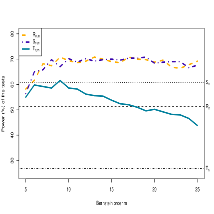
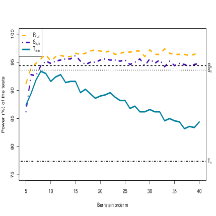
Figure 1: The power ($\%$) of the proposed tests versus the Bernstein polynomial order $m$. Left: Gumbel-Hougaard copula with sample size $n=100$; Right: Gumbel-Hougaard copula with sample size $n=200$.

4.2 Comparison with empirical beta copula-based test

The method of studying the effect of the Bernstein order $m$ in the preceding subsection is computationally expensive. In practice, one can apply the method suggested in Segers et al. (2017) to reduce the size of the grid of the Bernstein order $m.$ This recommendation will be used in order to compare the empirical power of the proposed testing procedure to the test based on the empirical beta copula denoted by $R_{n}^{\beta}$ in Kiriliouk et al. (2021). It was shown in Kiriliouk et al. (2021, Table 2.8) that the smoothed beta bootstrap test based on $R_{n}^{\beta}$ has slightly higher power in almost all cases. In Table 4 the same configuration for Clayton copula made asymmetric by Khoudraji’s device as in Kiriliouk et al. (2021, Table 2.8) was used. The table highlights the advantage of the empirical Bernstein copula-based tests using multiplier bootstraps on the smoothed beta bootstrap in almost all cases.

Remark 3.

Note that, the selection method of the Bernstein order $m$ recommended in Janssen et al. (2012) is not valid for the proposed multiplier bootstraps. Because this method of selection depends on the first and second partial derivatives of the underlying copula function $C$. Whereas for most copula models, these partial derivatives do not exist at the end points $(u,1),(1,u),(1,v),(v,1)$. Therefore, it fails to apply this approach for the second and third terms in Equation (8). It is also noted that this method of selection $m$ is valid only for interior points of $[0,1]^{2}$.

Table 4: Power ($\%$) of the tests of $\mathscr{H}_{0}$ based on $\{R_{n},S_{n},T_{n}\}$, $\{R_{n,m},S_{n,m},T_{n,m}\}$ and $R_{n}^{\beta}$, as estimated from $500$ samples from Clayton made asymmetric using Khoudraji’s device with $H=200$ multiplier replicates.

(n, m)	$\delta$	$\tau$	$R_{n}$	$R_{n,m}$	$S_{n}$	$S_{n,m}$	$T_{n}$	$T_{n,m}$	$R_{n}^{\beta}$
$\left(50,50/5\right)$	$1/4$	${0.25}$	$1.0$	$3.6$	$2.2$	3.8	$0.6$	$2.4$	$3.6$
		$0.50$	$2.0$	$5.4$	$5.4$	5.8	$1.2$	$1.8$	$5.4$
		$0.75$	$14.8$	$21.0$	41.8	$28.8$	$2.4$	$12.0$	$22.2$
	$1/2$	$0.25$	$0.8$	5.0	$4.2$	$4.8$	$0.4$	$2.4$	$4.8$
		$0.50$	$3.0$	$7.2$	$6.4$	7.4	$0.6$	$3.8$	$7.0$
		$0.75$	$24.8$	$45.8$	$48.2$	52.0	$5.2$	$29.6$	$44.0$
	$3/4$	$0.25$	$0.8$	4.4	$3.6$	$3.8$	$0.4$	$1.8$	$2.8$
		$0.50$	$2.0$	6.0	$5.6$	$5.8$	$1.0$	$2.6$	$5.8$
		$0.75$	$9.8$	21.4	$15.0$	21.4	$2.4$	$11.2$	$18.0$
$\left(100,100/5\right)$	$1/4$	${0.25}$	$1.8$	4.8	$2.4$	$4.4$	$2.6$	$3.8$	$4.0$
		$0.50$	$6.4$	$10.2$	$9.2$	11.0	$5.0$	$5.2$	$9.8$
		$0.75$	$51.4$	$62.6$	77.6	$71.2$	$25.2$	$40.6$	$64.4$
	$1/2$	$0.25$	$1.6$	$3.6$	$2.2$	4.0	$2.2$	$2.0$	$3.4$
		$0.50$	$8.8$	$16.8$	$14.0$	17.6	$5.8$	$10.4$	$14.0$
		$0.75$	$70.6$	$83.8$	$82.2$	86.2	$41.6$	$66.0$	$82.8$
	$3/4$	$0.25$	$3.2$	$5.6$	$5.2$	6.2	$2.6$	$3.4$	$4.4$
		$0.50$	$6.2$	$10.6$	$10.4$	12.2	$4.8$	$6.0$	$10.0$
		$0.75$	$30.0$	$40.2$	$36.4$	42.2	$20.2$	$28.6$	$38.2$

5 Real data application

5.1 Ocean data application

A simple illustration was carried out on the ocean data (at south Kodiak, Station $46066$) from the National Data Buoy Center (NDBC), US. There are three variables of interest: WVHT (significant wave height in meter), APD (average wave period in second) and WSPD (wind speed in meter per second) during the winter season of $2015$ (from November $2014$ to February $2015$) with $2855$ observations. Although the data was modelled using asymmetric copulas in Zhang et al. (2018), they did not provide a formal statistical test to justify the asymmetric structure therein. Here, the justification is shown using the empirical tests and the proposed Bernstein tests as in Table 5.

Rank plots are shown in Figure 2, one can notice that APD and WSPD are positively correlated with WVHT according to the Spearman’s rho. Further, as presented in Figure 3, these pairs most likely have an asymmetric dependence structure.

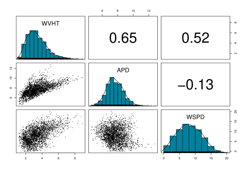
Figure 2: Scatter plot and Spearman’s rho between WVHT, APD and WSPD.

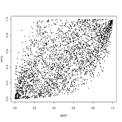
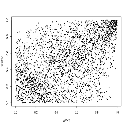
Figure 3: Rank plots of the pairs. Left: WVHT versus APD; Right: WVHT versus WSPD.

Table 5: P-values of the tests based on the empirical copula, the empirical Bernstein copula ($m_{1}=\lfloor n/100\rfloor,m_{2}=\lfloor n/50\rfloor$) and the empirical beta.

Pairs	$R_{n}$	$R_{n,m_{1}}$	$R_{n,m_{2}}$	$S_{n}$	$S_{n,m_{1}}$	$S_{n,m_{2}}$	$T_{n}$	$T_{n,m_{1}}$	$T_{n,m_{2}}$	$R_{n}^{\beta}$
(WVHT, APD)	$0.000$	$0.000$	$0.000$	$0.002$	$0.000$	$0.000$	$0.000$	$0.000$	$0.000$	$0.000$
(WVHT, WSPD)	$0.005$	$0.000$	$0.000$	$0.022$	$0.045$	$0.005$	$0.000$	$0.000$	$0.005$	$0.001$

To apply the proposed testing procedure, the Bernstein polynomial order was taken to be $m\in\left\{\lfloor 2118/100\rfloor,\right.$
$\left.\lfloor 2118/50\rfloor\right\}$, and other settings (the nominal level, number of multiplier bootstrap replicates $H$ and $20\times 20$ grids on $[0,1]^{2}$) were the same as in the simulation study. From Table 5, the Bernstein tests, empirical beta test and empirical tests reach the same conclusion that these two pairs have an asymmetric dependence pattern.

Once the asymmetric characteristic of dependence is confirmed, all the symmetric copula families (which is a huge proportion) should be ruled out for modelling. That is, to construct the copula function of $\rm{(WVHT,APD)}$ and $\rm{(WVHT,WSPD)}$, only asymmetric copulas should be considered. Naturally, one can use the Khoudraji’s device in Section 4 to obtain asymmetric copula models. In addition, there are various methods available in the literature, for example the product method in Liebscher (2008) and the linear convex combination method in Wu (2014).

5.2 Nutrient data application

A sample of daily intake (in mg) of calcium (Ca), iron (Fe), protein (Pr), vitamin A (vA) and vitamin C (vC) for $n=747$ women aged between 25 and 50 years has been collected by the United States Department of Agriculture in 1985. The nutrient data set (see also, Genest et al. (2012); Bahraoui et al. (2018)) is revisited to check the performance of the proposed Bernstein tests. In terms of the suggestion for Bernstein order $m$ in Segers et al. (2017), three candidates of $m$ are chosen, $i.e.$, $m=\left\{\lfloor n/30\rfloor=24,\lfloor n/70\rfloor=10,\lfloor n/90\rfloor=8\right\}$, with number of grids $N=20$.

To make a fair and concise comparison, the results of the characteristic function test $S_{n,\sigma^{*}}^{N}$ in Bahraoui et al. (2018) are also reported here as a competitor. Since P-values therein are computed based on a large amount of bootstraps, it is reasonable to consider a similarly large bootstrap sample, accordingly, $H=5000$ is considered in this subsection.

Table 6 indicates a surprisingly different conclusion of the Bernstein tests with $m=\lfloor n/70\rfloor$, that is, only Bernstein tests can reject the pair (Fe, vC) under $5\%$ nominal level. For other pairs, all the tests arrive at the same conclusion. Moreover, the time of calculating the P-values is also recorded based on a desktop PC with processor 11th Gen Intel(R) Core(TM) i5-11400F and graphics NVIDA GeForce RTX 3060 with $15$ repetitions (for time mean and standard deviation). It is important to emphasize that the $S_{n}$ test is conducted using the exchTest function within the R copula package, which is known for its high optimization. In terms of computational efficiency, the $S_{n,\sigma^{*}}^{N}$ test stands out as the most efficient choice.

Table 6: P-values and computational performance of empirical tests, empirical beta copula tests and Bernstein tests ($m_{1}=\lfloor n/30\rfloor,m_{2}=\lfloor n/70\rfloor,m_{3}=\lfloor n/90\rfloor$). Characteristic function test $S^{N}_{n,\sigma^{*}}$ in Bahraoui et al. (2018) is also reported here.

	Pair	Statistics
		$R_{n}$	$R_{n,m_{1}}$	$R_{n,m_{2}}$	$R_{n,m_{3}}$	$S_{n}$	$S_{n,m_{1}}$	$S_{n,m_{2}}$	$S_{n,m_{3}}$	$T_{n}$	$T_{n,m_{1}}$	$T_{n,m_{2}}$	$T_{n,m_{3}}$	$R_{n}^{\beta}$	$S^{N}_{n,\sigma^{*}}$
P-values	(Ca, Fe)	0.010	0.005	0.007	0.000	0.003	0.005	0.008	0.000	0.002	0.006	0.007	0.000	0.006	0.004
	(Ca, Pr)	0.000	0.000	0.000	0.000	0.000	0.000	0.000	0.000	0.001	0.000	0.000	0.000	0.000	$0.000$
	(Ca, vA)	0.000	0.000	0.000	0.000	0.000	0.000	$0.000$	0.000	0.000	0.000	0.000	0.000	0.000	0.000
	(Ca, vC)	0.143	0.166	0.321	0.216	0.158	0.169	0.317	0.223	0.065	0.092	0.276	0.171	0.151	$0.225$
	(Fe, Pr)	0.304	0.796	0.956	0.996	0.394	0.678	0.954	0.993	0.114	0.529	0.943	0.998	0.501	$0.895$
	(Fe, vA)	0.003	0.004	0.022	0.005	0.000	0.004	0.017	0.005	0.005	0.002	0.009	0.002	0.001	$0.008$
	(Fe, vC)	0.008	0.006	0.012	0.004	0.005	0.005	0.009	0.004	0.012	0.012	0.013	0.004	0.007	$0.007$
	(Pr, vA)	0.007	0.006	0.029	0.003	0.001	0.005	0.020	0.002	0.024	0.013	0.029	0.004	0.005	$0.006$
	(Pr, vC)	0.194	0.092	$\mathbf{0.036}$	0.143	0.112	0.089	$\mathbf{0.034}$	0.133	0.070	0.240	0.052	0.147	0.153	$0.064$
	(vA, vC)	0.549	0.834	0.884	0.927	0.602	0.828	0.884	0.922	0.180	0.774	0.913	0.940	0.624	$0.827$
Time	(Ca, Fe)	16.083	159.849	30.219	20.336	24.947	434.192	81.676	54.421	22.694	168.899	35.939	25.630	$640.700$	9.014
mean	(Ca, Pr)	15.973	159.809	30.560	20.378	24.818	433.909	82.875	54.546	22.779	168.868	35.902	25.256	$830.757$	8.904
(secs)	(Ca, vA)	15.987	159.800	29.610	20.204	24.807	438.175	79.886	55.000	25.505	186.549	34.852	25.584	$613.265$	8.276
	(Ca, vC)	16.710	163.675	29.626	19.996	26.679	442.293	79.889	53.352	23.705	171.107	34.833	24.712	$631.973$	8.237
	(Fe, Pr)	16.327	160.460	29.553	19.883	25.110	435.617	79.913	53.364	23.062	169.563	34.848	24.661	$765.784$	8.238
	(Fe, vA)	16.230	168.632	29.685	19.863	31.671	455.719	79.912	53.367	23.760	172.449	34.846	24.638	$594.638$	8.183
	(Fe, vC)	16.880	170.615	29.549	19.960	32.841	444.503	79.911	53.339	22.883	169.118	34.806	24.664	$570.436$	8.182
	(Pr, vA)	17.143	159.834	29.605	19.933	25.050	460.171	79.893	53.344	28.486	174.660	34.825	24.637	$556.674$	8.309
	(Pr, vC)	17.843	175.920	29.651	20.661	27.116	439.817	79.898	55.361	23.242	170.081	34.830	24.671	$565.487$	8.470
	(vA, vC)	16.571	160.764	29.589	20.425	27.435	461.440	79.921	54.761	28.622	171.081	34.799	24.686	$608.412$	8.416
Time	(Ca, Fe)	0.080	0.206	0.085	0.118	0.098	1.216	0.577	0.271	0.027	0.129	0.242	0.589	$66.092$	0.223
standard	(Ca, Pr)	0.059	0.106	0.244	0.059	0.057	0.120	0.596	0.295	0.063	0.110	0.237	0.231	$212.529$	0.175
deviation	(Ca, vA)	0.067	0.087	0.062	0.317	0.053	4.873	0.075	0.448	1.605	6.344	0.090	0.324	$36.873$	0.324
	(Ca, vC)	0.073	0.929	0.082	0.073	0.227	2.589	0.047	0.091	0.128	1.348	0.070	0.143	$81.312$	0.114
	(Fe, Pr)	0.067	0.093	0.014	0.014	0.087	0.115	0.102	0.066	0.038	0.130	0.091	0.121	$114.724$	0.121
	(Fe, vA)	0.121	7.014	0.064	0.076	2.718	19.865	0.065	0.065	0.053	0.926	0.099	0.097	$62.509$	0.079
	(Fe, vC)	0.238	7.008	0.013	0.100	0.409	13.617	0.123	0.072	0.065	0.154	0.108	0.141	$7.012$	0.067
	(Pr, vA)	0.708	0.129	0.053	0.092	0.101	24.851	0.068	0.042	0.384	2.948	0.096	0.100	$5.417$	0.143
	(Pr, vC)	0.351	4.343	0.124	0.177	0.485	12.610	0.062	0.287	0.147	0.449	0.080	0.142	$7.623$	0.271
	(vA, vC)	0.277	0.376	0.047	0.139	0.157	27.036	0.128	0.198	0.505	1.337	0.121	0.097	$82.739$	0.119

The bold values indicate a different decision for Bernstein tests comparing with other tests under $5\%$ nominal level.

6 Final remarks

Tests based on the Bernstein polynomials for symmetry of bivariate copulas were proposed and investigated. These test statistics are smoothed versions of those based on the empirical copula in Genest et al. (2012). The proposed procedure exhibits enhanced performance in simulation studies and aligns with identical conclusions in real data applications across the majority of scenarios. The limiting distributions of the proposed test statistics were investigated and a Bernstein version of multiplier bootstrap was constructed and implemented to simulate P-values.

Since the underlying copula is continuous, a smooth copula estimator such as the empirical Bernstein copula is competitive with the empirical copula. From the bias-variance trade-off point of view, with appropriate smoothness parameter, the former can outperform the latter by balancing the bias and variance. On the other hand, the smoothed Bernstein tests still hold the same features as the non-smoothed empirical tests. For example, the empirical tests tend to have an empirical level which is below the nominal level, see Genest et al. (2012) and  Bahraoui et al. (2018). The proposed Bernstein tests still undergo this pattern, but are less affected.

For future study, it would be possible to apply the Bernstein polynomials for testing various kinds of symmetry in Nelsen (1993) and the vertex and diametrical symmetry developed in Mangold (2017) recently. In general, other statistical tests based on the empirical copula can be adapted easily to use the empirical Bernstein copula. Another avenue to explore involves adopting distinct Bernstein orders for each component of the empirical Bernstein copula. Drawing from the authors’ experiential insights, such alternatives are likely to offer benefits, particularly concerning $R_{n,m}$ and $T_{n,m}$.

7 Acknowledgements

M. Belalia gratefully acknowledge the research support of the Natural Sciences and Engineering Research Council of Canada(RGPIN/05496-2020 ).

Appendix A Proof of Theorem 2

Proof.

This proof is an adaption of Genest et al. (2012, Proposition 3). For the convergence of $nR_{n,m}$ and $n^{1/2}T_{n,m}$, one can directly apply continuous mapping theorem combined with Theorem 1. For the convergence of $nS_{n,m}$, the functional delta method was used. To this end, let $\mathscr{C}[0,1]^{2}$ denote the space of continuous functions on $[0,1]^{2}$, $\mathscr{D}[0,1]^{2}$ denote the space of functions with continuity from upper right quadrant and limits from other quadrants on $[0,1]^{2}$, equipped with sup-norm. Further, denote $\rm{BV}_{1}[0,1]^{2}$ by the subspace of $\mathscr{D}[0,1]^{2}$ where functions with total variation bounded by $1$. By continuous mapping theorem,

$$\left(\mathbb{S}^{2}_{n,m},\mathbb{B}_{n,m}\right)\rightsquigarrow\left(\mathbb{S}_{C}^{2},\mathbb{B}_{C}\right)$$

in the space $\ell^{\infty}[0,1]^{2}\times\ell^{\infty}[0,1]^{2}$. Rewrite it as

$$\left(\mathbb{S}^{2}_{n,m},\mathbb{B}_{n,m}\right)=n^{1/2}\{(A_{n,m},\widehat{C}_{n,m})-(A,C)\},$$

where $A\equiv 0$ and $A_{n,m}\mathrel{\mathop{\ordinarycolon}}=n^{1/2}(\widehat{C}_{n,m}-\widehat{C}_{n,m}^{\top})^{2}$, where $\widehat{C}_{n,m}^{\top}(u,v)=\widehat{C}_{n,m}(v,u)$. Then, consider the map $\phi\mathrel{\mathop{\ordinarycolon}}\ell^{\infty}[0,1]^{2}\times\rm{BV}_{1}[0,1]^{2}\to{\mathbb{R}}$ defined by

$$\phi(a,b)=\int_{(0,1]^{2}}a\operatorname{d\!}b,$$

Clearly,

$$nS_{n,m}=\phi\left(\mathbb{S}^{2}_{n,m},\mathbb{B}_{n,m}\right)=n^{1/2}\{\phi(A_{n,m},\widehat{C}_{n,m})-\phi(A,C)\}.$$

To conclude the proof, by Carabarin-Aguirre and Ivanoff (2010, Lemma 4.3), $\phi$ is Hadamard differentiable tangentially to $\mathscr{C}[0,1]^{2}\times\mathscr{D}[0,1]^{2}$ at each $(\alpha,\beta)$ in $\ell^{\infty}[0,1]^{2}\times\rm{BV}_{1}[0,1]^{2}$ such that $\int|d\alpha|<\infty$ with derivative

$$\phi^{\prime}_{(\alpha,\beta)}(a,b)=\int\alpha\operatorname{d\!}b+\int a\operatorname{d\!}\beta.$$

Then by applying the Functional Delta Method (van der Vaart and Wellner, 1996, Theorem 3.9.4), $nS_{n,m}\rightsquigarrow\phi^{\prime}_{(A,C)}\left(\mathbb{S}_{C}^{2},\mathbb{B}_{C}\right)$, where

$$\phi^{\prime}_{(A,\,C)}\left(\mathbb{S}_{C}^{2},\mathbb{B}_{C}\right)=\int_{(0,1]^{2}}A\operatorname{d\!}\mathbb{B}_{C}+\int_{(0,1]^{2}}\mathbb{S}_{C}^{2}\operatorname{d\!}C=\int_{(0,1]^{2}}\mathbb{S}_{C}^{2}\operatorname{d\!}C.$$

This yields to the desired result. ∎

Appendix B Proof of Theorem 3

Proof.

This proof is an adaption of Genest et al. (2012, Proposition 4). The strongly uniform consistency of $\widehat{C}_{n,m}$ was provided in Janssen et al. (2012, Theorem 1), then by continuous mapping theorem, it follows immediately that $R_{n,m}$ and $T_{n,m}$ converge to $R_{C}$ and $T_{C}$ almost surely, respectively. Further, to prove the convergence of $S_{n,m}$, write

$$|S_{n,m}-S_{C}|\leq|\gamma_{n,m}|+|\zeta_{n}|,$$

where

$$\gamma_{n,m} =\int_{0}^{1}\int_{0}^{1}\left\{\widehat{C}_{n,m}(u,v)-\widehat{C}_{n,m}(v,u)\right\}^{2}\operatorname{d\!}\widehat{C}_{n}(u,v)$$

$$\quad-\int_{0}^{1}\int_{0}^{1}\left\{{C}(u,v)-{C}(v,u)\right\}^{2}\operatorname{d\!}\widehat{C}_{n}(u,v),$$

and

$$\zeta_{n} =\int_{0}^{1}\int_{0}^{1}\left\{{C}(u,v)-{C}(v,u)\right\}^{2}\operatorname{d\!}\widehat{C}_{n}(u,v)-\int_{0}^{1}\int_{0}^{1}\left\{{C}(u,v)-{C}(v,u)\right\}^{2}\operatorname{d\!}{C}(u,v).$$

Since

$$\left|\left\{\widehat{C}_{n,m}(u,v)-\widehat{C}_{n,m}(v,u)\right\}^{2}-\left\{C(u,v)-C(v,u)\right\}^{2}\right|$$

$$=\left|\left[\widehat{C}_{n,m}(u,v)+C(u,v)\right]-\left[\widehat{C}_{n,m}(v,u)+C(v,u)\right]\right|$$

$$\quad\times\left|\left[\widehat{C}_{n,m}(u,v)-C(u,v)\right]-\left[\widehat{C}_{n,m}(v,u)-C(v,u)\right]\right|$$

$$\leq\left[\left|\widehat{C}_{n,m}(u,v)+C(u,v)\right|+\left|\widehat{C}_{n,m}(v,u)+C(v,u)\right|\right]$$

$$\quad\times\left[\left|\widehat{C}_{n,m}(u,v)-C(u,v)\right|+\left|\widehat{C}_{n,m}(v,u)-C(v,u)\right|\right]$$

$$\leq 8\sup_{(u,v)\in[0,1]^{2}}\left|\widehat{C}_{n,m}(u,v)-C(u,v)\right|,$$

one has

$$|\gamma_{n,m}|\leq 8\sup_{(u,v)\in[0,1]^{2}}\left|\widehat{C}_{n,m}(u,v)-C(u,v)\right|\xrightarrow{a.s.}0.$$

For $\zeta_{n}$, by Genest et al. (1995, Proposition A.1 (i)), one has

$$\int_{0}^{1}\int_{0}^{1}\left\{{C}(u,v)-{C}(v,u)\right\}^{2}\operatorname{d\!}\widehat{C}_{n}(u,v)\rightarrow\int_{0}^{1}\int_{0}^{1}\left\{{C}(u,v)-{C}(v,u)\right\}^{2}\operatorname{d\!}{C}(u,v),$$

then $\zeta_{n}\rightarrow 0$. Therefore, $S_{n,m}$ converges to $S_{C}$ almost surely. ∎

Appendix C Proof of Lemma 1

Proof.

Under these assumptions, one need to use the framework in Segers et al. (2017). Specifically, let $\mu_{m,(u,v)}$ be the law of random vector $(B_{1}/m,B_{2}/m)$, where $B_{1}$ and $B_{2}$ follow $\textsf{Binomial}(m,u)$ and $\textsf{Binomial}(m,v)$, respectively. The empirical Bernstein copula can be rewritten as

$$\widehat{C}_{n,m}(u,v)=\int_{[0,1]^{2}}\widehat{C}_{n}(x,y)\,{\rm d}\mu_{m,(u,v)}(x,y),\qquad(x,y)\in[0,1]^{2}.$$

Moreover, write $(x,y)(t)=(u,v)+t((x,y)-(u,v))$ with $t\in[0,1]$. Then, the empirical Bernstein copula process is

$$\mathbb{B}_{n,m}(u,v) =\sqrt{n}\left\{\widehat{C}_{n,m}(u,v)-C(u,v)\right\}$$

$$=\sqrt{n}\left\{\widehat{C}_{n,m}(u,v)-\int_{[0,1]^{2}}C(x,y)\,{\rm d}\mu_{m,(u,v)}(x,y)+\int_{[0,1]^{2}}C(x,y)\,{\rm d}\mu_{m,(u,v)}(x,y)-C(u,v)\right\}$$

$$=\int_{[0,1]^{2}}\sqrt{n}\left\{\widehat{C}_{n,m}(x,y)-C(x,y)\right\}\,{\rm d}\mu_{m,(u,v)}(x,y)+\sqrt{n}\left\{\int_{[0,1]^{2}}C(x,y)\,{\rm d}\mu_{m,(u,v)}(x,y)-C(u,v)\right\}$$

$$=T_{1}+T_{2}.$$ (9)

The two terms are dealt with separately.

• For the term $T_{1}$, according to Segers et al. (2017, Proposition 3.1), one has

  $$\sup\limits_{(u,v)\in[0,1]^{2}}\left|\int_{[0,1]^{2}}\sqrt{n}\left\{\widehat{C}_{n,m}(s,t)-C(s,t)\right\}\,{\rm d}\mu_{m,(u,v)}(s,t)-\sqrt{n}\left\{\widehat{C}_{n,m}(u,v)-C(u,v)\right\}\right|=o_{p}(1).$$

  And note that, $\sqrt{n}\left\{\widehat{C}_{n,m}(u,v)-C(u,v)\right\}\rightsquigarrow\mathbb{B}_{C}(u,v)$ in $\ell^{\infty}([0,1]^{2})$ under the Assumption 1 (see Segers (2012)). Therefore, $T_{1}\rightsquigarrow\mathbb{B}_{C}(u,v)$ as $n$ goes to infinity.

• For the term $T_{2}$, Let $m=cn^{\alpha}$ for some $c>0$, by Kojadinovic (2022, Lemma 3.1),under Assumption 1-2 , one has

  $$\sup_{(u,v)\in[0,1]^{2}}\sqrt{n}\left|\int_{[0,1]^{2}}C(x,y)\,{\rm d}\mu_{m,(u,v)}(x,y)-C(u,v)\right|=O\left(n^{(3-4\alpha)/6}\right)$$

  almost surely. Therefore, if $\alpha>3/4$, $T_{2}$ goes to zero as $n$ goes to infinity.

Combining above results completes the proof. ∎

Appendix D Proof of Proposition 1

Proof.

By Rémillard and Scaillet (2009), one has

$$\mathbb{C}_{n}(u,v)=\sqrt{n}\left\{C_{n}(u,v)-C(u,v)\right\} =n^{1/2}\Bigg{\{}\frac{1}{n}\sum_{i=1}^{n}\left\{{\mathbb{I}}\left(U_{i}\leq u,V_{i}\leq v)-C(u,v\right)\right\}\Bigg{\}}$$

$$\quad\rightsquigarrow\mathbb{C}(u,v),$$

where $C_{n}(u,v)=\frac{1}{n}\sum_{i=1}^{n}{\mathbb{I}}\left(U_{i}\leq u,V_{i}\leq v\right)$, and

$$\overline{\mathbb{C}}^{(h)}_{n}(u,v) =n^{1/2}\Bigg{\{}\frac{1}{n}\sum_{i=1}^{n}\left(\xi^{(h)}_{i}-\bar{\xi}_{n}^{(h)}\right){\mathbb{I}}(\widehat{U}_{i}\leq u,\widehat{V}_{i}\leq v)\Bigg{\}}\rightsquigarrow\mathbb{C}(u,v).$$

To end the proof, one needs to show that the difference between $\left(\mathbb{C}_{n},\overline{\mathbb{C}}^{(h)}_{n}\right)$ and $\left(\widetilde{\mathbb{B}}_{n,m},\overline{\mathbb{B}}^{(h)}_{n,m}\right)$ are asymptotically negligible.

It is well-known (for example, see Deheuvels (1979)) that, as $n\to\infty$,

$$\|C_{n}(u,v)-C(u,v)\|=O\left(n^{-1/2}(\log\log n)^{1/2}\right),$$

almost surely and using the same techniques in Janssen et al. (2012) gives

$$\|C_{n,m}(u,v)-C(u,v)\|=O\left(n^{-1/2}(\log\log n)^{1/2}\right),$$

almost surely, it immediately follows that

$$\|C_{n,m}(u,v)-C_{n}(u,v)\|=O\left(n^{-1/2}(\log\log n)^{1/2}\right),$$

almost surely. Therefore, one can conclude that $\widetilde{\mathbb{B}}_{n,m}(u,v)\rightsquigarrow\mathbb{C}(u,v)$.

Further, by Janssen et al. (2012, Lemma 1), as $n\to\infty$,

$$\|\widehat{C}_{n}(u,v)-C(u,v)\| =O\left(n^{-1/2}(\log\log n)^{1/2}\right),$$

almost surely. By Lemma 1, under the assumptions,

$$\|\widehat{C}_{n,m}(u,v)-C(u,v)\|=o_{p}(1).$$

Hence

$$\|\widehat{C}_{n,m}(u,v)-\widehat{C}_{n}(u,v)\|=o_{p}(1),$$

one has that $\overline{\mathbb{B}}_{n,m}^{(h)}(u,v)\rightsquigarrow\mathbb{C}(u,v)$. ∎

Appendix E Proof of Proposition 2

Proof.

We only show the uniform consistency for

$$\frac{\partial\widehat{C}_{n,m}(u,v)}{\partial u} =m\sum_{k=0}^{m-1}\sum_{\ell=0}^{m}\bigg{\{}\widehat{C}_{n}\left(\frac{k+1}{m},\frac{\ell}{m}\right)-\widehat{C}_{n}\left(\frac{k}{m},\frac{\ell}{m}\right)\bigg{\}}$$

$$\quad\cdot P_{m-1,k}(u)P_{m,\ell}(v).$$

The result for the other partial derivative can be obtained similarly. For any $u\in[b_{n},1-b_{n}],v\in[0,1]$, one has

$$\left|\frac{\partial\widehat{C}_{n,m}(u,v)}{\partial u}-\dot{C}_{1}(u,v)\right|$$

$$\quad\leq\Bigg{|}m\sum_{k=0}^{m-1}\sum_{\ell=0}^{m}\bigg{\{}\widehat{C}_{n}\left(\frac{k+1}{m},\frac{\ell}{m}\right)-\widehat{C}_{n}\left(\frac{k}{m},\frac{\ell}{m}\right)$$

$$\qquad-{C}\left(\frac{k+1}{m},\frac{\ell}{m}\right)+{C}\left(\frac{k}{m},\frac{\ell}{m}\right)\bigg{\}}P_{m-1,k}(u)P_{m,\ell}(v)\Bigg{|}$$

$$\qquad+\Bigg{|}m\sum_{k=0}^{m-1}\sum_{\ell=0}^{m}\bigg{\{}{C}\left(\frac{k+1}{m},\frac{\ell}{m}\right)-{C}\left(\frac{k}{m},\frac{\ell}{m}\right)\bigg{\}}$$

$$\qquad\cdot P_{m-1,k}(u)P_{m,\ell}(v)-\dot{C}_{1}(u,v)\Bigg{|}$$

$$\quad=A_{1}+A_{2}.$$

Further, let $P_{m,k}^{\prime}(u)=\frac{1}{u(1-u)}P_{m,k}(u)\left(k-mu\right)$ be the derivative of $P_{m,k}(u)$, then

$$A_{1} \leq\sum_{k=0}^{m}\sum_{\ell=0}^{m}\bigg{|}\widehat{C}_{n}\left(\frac{k}{m},\frac{\ell}{m}\right)-{C}\left(\frac{k}{m},\frac{\ell}{m}\right)\bigg{|}$$

$$\quad\cdot\left|P_{m,k}^{\prime}(u)\right|P_{m,\ell}(v)$$

$$\leq\sup_{(u,v)\in[0,1]^{2}}\bigg{|}\widehat{C}_{n}\left(u,v\right)-{C}\left(u,v\right)\bigg{|}\cdot\sum_{k=0}^{m}\left|P_{m,k}^{\prime}(u)\right|$$

$$=O\left(m^{1/2}n^{-1/2}(\log\log n)^{1/2}\right),$$

almost surely as $n\to\infty$ and where

$$\sum_{k=0}^{m}\left|P_{m,k}^{\prime}(u)\right|=O(m^{1/2}),$$

by Janssen et al. (2014, Lemma 1).

For dealing with $A_{2}$, let $\nu_{m,(u,v)}$ be the law of random vector $(S_{1}/(m-1),S_{2}/m)$, where $S_{1}$ and $S_{2}$ follow $\textsf{Binomial}(m-1,u)$ and $\textsf{Binomial}(m,v)$, respectively. Therefore,

$$\sum_{k=0}^{m-1}\sum_{\ell=0}^{m}C\left(\frac{k+1}{m},\frac{\ell}{m}\right)P_{m-1,k}(u)P_{m,\ell}(v)$$

$$\quad=\int_{[0,1]^{2}}C\left(\left(x+\frac{1}{m-1}\right)\frac{m-1}{m},y\right)$$

$$\qquad\operatorname{d\!}\nu_{m,(u,v)}(x,y),$$

and

$$\sum_{k=0}^{m-1}\sum_{\ell=0}^{m}C\left(\frac{k}{m},\frac{\ell}{m}\right)P_{m-1,k}(u)P_{m,\ell}(v)$$

$$\quad=\int_{[0,1]^{2}}C\left(x\frac{m-1}{m},y\right)\operatorname{d\!}\nu_{m,(u,v)}(x,y).$$

Using the representation in Segers et al. (2017, Proof of Proposition 3.4), for $0<t<1$, one has

$$A_{2} =\Bigg{|}m\sum_{k=0}^{m-1}\sum_{\ell=0}^{m}\bigg{\{}{C}\left(\frac{k+1}{m},\frac{\ell}{m}\right)-{C}\left(\frac{k}{m},\frac{\ell}{m}\right)\bigg{\}}$$

$$\quad\cdot P_{m-1,k}(u)P_{m,\ell}(v)-\dot{C}_{1}(u,v)\Bigg{|}$$

$$=\left|\int_{0}^{1}\bigg{\{}\int_{[0,1]^{2}}\left[\dot{C}_{1}\left(\frac{m-1}{m}x+\frac{1+t}{m},y\right)-\dot{C}_{1}(u,v)\right]\right.$$

$$\quad\left.{\rm d}\nu_{m,(u,v)}(x,y)\bigg{\}}{\rm d}t\right|.$$ (10)

Let $x^{\prime}(x,t)\mathrel{\mathop{\ordinarycolon}}=\frac{m-1}{m}x+\frac{1+t}{m}$ and $\varepsilon_{n}=b_{n}/2$, then one has,

$$\eqref{eq:2023-08-28, 1:05PM} \leq\left|\int_{0}^{1}\bigg{\{}\int_{[0,1]^{2}}\left[\dot{C}_{1}\left(x^{\prime},y\right)-\dot{C}_{1}(u,v)\right]\right.$$

$$\quad\cdot{\mathbb{I}}\left(\max(|x^{\prime}-u|,|y-v|)\leq\varepsilon_{n}\right)$$

$$\quad\left.\operatorname{d\!}\nu_{m,(u,v)}(x,y)\bigg{\}}\operatorname{d\!}t\right|$$

$$\quad+\left|\int_{0}^{1}\bigg{\{}\int_{[0,1]^{2}}\left[\dot{C}_{1}\left(x^{\prime},y\right)-\dot{C}_{1}(u,v)\right]\right.$$

$$\quad\left.\cdot{\mathbb{I}}\left(\max(|x^{\prime}-u|,|y-v|)>\varepsilon_{n}\right)\operatorname{d\!}\nu_{m,(u,v)}(x,y)\bigg{\}}{\rm d}t\right|$$

$$=A_{21}+A_{22}.$$

Further, the two terms are dealt with separately using the strategy in Kojadinovic (2022, Proof of Lemma 3.1).

• For $A_{21}$, under Assumption 1-2, by Segers (2012, Lemma 4.3), for a constant $L>0$, one has

  $$\left|\dot{C}_{1}\left(x^{\prime},y\right)-\dot{C}_{1}(u,v)\right|{\mathbb{I}}\left(\max(|x^{\prime}-u|,|y-v|)\leq\varepsilon_{n}\right)$$

  $$\quad\leq Lb_{n}^{-1}\left[|x^{\prime}-u|+|y-v|\right].$$

  Further,

  $$A_{21} \leq Lb_{n}^{-1}\int_{0}^{1}\bigg{\{}\int_{[0,1]^{2}}\left[|x^{\prime}-u|+|y-v|\right]$$

  $$\quad{\rm d}\nu_{m,(u,v)}(x,y)\bigg{\}}\operatorname{d\!}t$$

  $$\leq Lb_{n}^{-1}\int_{[0,1]^{2}}\int_{0}^{1}\left[|x-u|+|y-v|+\left|\frac{x}{m}-\frac{1+t}{m}\right|\right]$$

  $$\quad\operatorname{d\!}t\operatorname{d\!}\nu_{m,(u,v)}(x,y)$$

  $$\leq Lb_{n}^{-1}\int_{[0,1]^{2}}\int_{0}^{1}\left[|x-u|+|y-v|\right.$$

  $$\quad\left.+\frac{x}{m}+\frac{1+t}{m}\right]\operatorname{d\!}t\operatorname{d\!}\nu_{m,(u,v)}(x,y)$$

  $$=Lb_{n}^{-1}\int_{[0,1]^{2}}\left[|x-u|+|y-v|+\frac{x}{m}+\frac{3}{2m}\right]\operatorname{d\!}\nu_{m,(u,v)}(x,y).$$ (11)

  By Cauchy-Schwarz inequality,

  $$\eqref{eq:2023-08-28, 2:20PM} \leq Lb_{n}^{-1}\left[O\left(m^{-1/2}\right)+O(m^{-1})\right]$$

  $$=O\left(b_{n}^{-1}m^{-1/2}\right).$$

• For $A_{22}$, since $0\leq\dot{C}_{1}\leq 1$ and using the result of $A_{21}$,

  $$A_{22} \leq\left|\int_{0}^{1}\bigg{\{}\int_{[0,1]^{2}}\frac{2}{\varepsilon_{n}}\max(|x^{\prime}-u|,|y-v|)\right.$$

  $$\quad\left.\operatorname{d\!}\nu_{m,(u,v)}(x,y)\bigg{\}}{\rm d}t\right|$$

  $$\leq\left|\int_{0}^{1}\bigg{\{}\int_{[0,1]^{2}}\frac{2}{\varepsilon_{n}}(|x^{\prime}-u|+|y-v|)\right.$$

  $$\quad\left.\operatorname{d\!}\nu_{m,(u,v)}(x,y)\bigg{\}}{\rm d}t\right|$$

  $$\leq\varepsilon_{n}^{-1}\left[O\left(m^{-1/2}\right)+O(m^{-1})\right]$$

  $$=O\left(b_{n}^{-1}m^{-1/2}\right).$$

Therefore,

$$\sup_{\begin{subarray}{c}v\in[0,1],\\ u\in[b_{n},1-b_{n}]\end{subarray}}\left|\frac{\partial\widehat{C}_{n,m}(u,v)}{\partial u}-\dot{C}_{1}(u,v)\right|$$

$$\quad=O\left(m^{1/2}n^{-1/2}(\log\log n)^{1/2}\right)+O\left(b_{n}^{-1}m^{-1/2}\right),$$

almost surely as $n\to\infty$, which completes the proof. ∎

References

• Bahraoui et al. (2018) Bahraoui, T., T. Bouezmarni, and J.-F. Quessy (2018). Testing the symmetry of a dependence structure with a characteristic function. Dependence Modeling 6(1), 331–355.
• Bahraoui and Quessy (2022) Bahraoui, T. and J.-F. Quessy (2022). Tests of multivariate copula exchangeability based on Lévy measures. Scandinavian Journal of Statistics 49(3), 1215–1243.
• Beare and Seo (2020) Beare, B. K. and J. Seo (2020). Randomization tests of copula symmetry. Econometric Theory 36(6), 1025–1063.
• Belalia (2016) Belalia, M. (2016). On the asymptotic properties of the Bernstein estimator of the multivariate distribution function. Statistics and Probability Letters 110, 249–256.
• Belalia et al. (2017) Belalia, M., T. Bouezmarni, F. C. Lemyre, and A. Taamouti (2017). Testing independence based on Bernstein empirical copula and copula density. Journal of Nonparametric Statistics 29(2), 346–380.
• Carabarin-Aguirre and Ivanoff (2010) Carabarin-Aguirre, A. and B. G. Ivanoff (2010). Estimation of a distribution under generalized censoring. Journal of Multivariate Analysis 101(6), 1501–1519.
• Chen and Huang (2007) Chen, S. X. and T.-M. Huang (2007). Nonparametric estimation of copula functions for dependence modelling. Canadian Journal of Statistics 35(2), 265–282.
• Cousido-Rocha et al. (2019) Cousido-Rocha, M., J. de Uña-Álvarez, and J. D. Hart (2019). A two-sample test for the equality of univariate marginal distributions for high-dimensional data. Journal of Multivariate Analysis 174, 104537.
• Deheuvels (1979) Deheuvels, P. (1979). La fonction de dépendance empirique et ses propriétés. Un test non paramétrique d’indépendance. Bulletins de l’Académie Royale de Belgique 65, 274–292.
• Fermanian et al. (2004) Fermanian, J.-D., D. Radulović, and M. Wegkamp (2004). Weak convergence of empirical copula processes. Bernoulli 10(5), 847–860.
• Fujii (1989) Fujii, Y. (1989). Test for the equality of marginal distributions on positively dependent bivariate survival data. Communications in Statistics-Simulation and Computation 18(2), 633–642.
• Genest et al. (1995) Genest, C., K. Ghoudi, and L.-P. Rivest (1995). A semiparametric estimation procedure of dependence parameters in multivariate families of distributions. Biometrika 82(3), 543–552.
• Genest et al. (2012) Genest, C., J. Nešlehová, and J.-F. Quessy (2012). Tests of symmetry for bivariate copulas. Annals of the Institute of Statistical Mathematics 64(4), 811–834.
• Genest et al. (2017) Genest, C., J. G. Nešlehová, and B. Rémillard (2017). Asymptotic behavior of the empirical multilinear copula process under broad conditions. Journal of Multivariate Analysis 159, 82–110.
• Genest et al. (2009) Genest, C., B. Remillard, and D. Beaudoin (2009). Goodness-of-fit tests for copulas: A review and a power study. Insurance: Mathematics and Economics 44(2), 199–213.
• Gijbels and Mielniczuk (1990) Gijbels, I. and J. Mielniczuk (1990). Estimating the density of a copula function. Communications in Statistics-Theory and Methods 19(2), 445–464.
• Grimaldi and Serinaldi (2006) Grimaldi, S. and F. Serinaldi (2006). Asymmetric copula in multivariate flood frequency analysis. Advances in Water Resources 29(8), 1155–1167.
• Harder and Stadtmüller (2017) Harder, M. and U. Stadtmüller (2017). Testing exchangeability of copulas in arbitrary dimension. Journal of Nonparametric Statistics 29(1), 40–60.
• Hofert et al. (2023) Hofert, M., I. Kojadinovic, M. Maechler, and J. Yan (2023). copula: Multivariate Dependence with Copulas. R package version 1.1-2.
• Janssen et al. (2012) Janssen, P., J. Swanepoel, and N. Veraverbeke (2012). Large sample behavior of the Bernstein copula estimator. Journal of Statistical Planning and Inference 142(5), 1189–1197.
• Janssen et al. (2014) Janssen, P., J. Swanepoel, and N. Veraverbeke (2014). A note on the asymptotic behavior of the Bernstein estimator of the copula density. Journal of Multivariate Analysis 124, 480–487.
• Janssen et al. (2016) Janssen, P., J. Swanepoel, and N. Veraverbeke (2016). Bernstein estimation for a copula derivative with application to conditional distribution and regression functionals. Test 25(2), 351–374.
• Jaser and Min (2021) Jaser, M. and A. Min (2021). On tests for symmetry and radial symmetry of bivariate copulas towards testing for ellipticity. Computational Statistics 36(3), 1–26.
• Khoudraji (1995) Khoudraji, A. (1995). Contributions à l’étude des copules et à la modélisation de valeurs extrêmes bivariées. Ph. D. thesis, Université Laval, Québec, Canada.
• Kiriliouk et al. (2021) Kiriliouk, A., J. Segers, and H. Tsukahara (2021). Resampling procedures with empirical beta copulas. In Pioneering Works on Extreme Value Theory: In Honor of Masaaki Sibuya, pp.  27–53. Springer.
• Kojadinovic (2022) Kojadinovic, I. (2022). On Stute’s representation for a class of smooth, possibly data-adaptive empirical copula processes. arXiv preprint arXiv:2204.11240.
• Kojadinovic and Yi (2021) Kojadinovic, I. and B. Yi (2021). A class of smooth, possibly data-adaptive nonparametric copula estimators containing the empirical beta copula. arXiv preprint arXiv:2106.10726.
• Leblanc (2012) Leblanc, A. (2012). On the boundary properties of Bernstein polynomial estimators of density and distribution functions. Journal of Statistical Planning and Inference 142(10), 2762–2778.
• Liebscher (2008) Liebscher, E. (2008). Construction of asymmetric multivariate copulas. Journal of Multivariate Analysis 99(10), 2234–2250.
• Mangold (2017) Mangold, B. (2017). New concepts of symmetry for copulas. Technical report, FAU Discussion Papers in Economics.
• Morettin et al. (2010) Morettin, P. A., C. M. C. Toloi, C. Chiann, and J. C. S. de Miranda (2010). Wavelet-smoothed empirical copula estimators. Revista Brasileira de Finanças 8(3), 263–281.
• Nelsen (1993) Nelsen, R. B. (1993). Some concepts of bivariate symmetry. Journal of Nonparametric Statistics 3(1), 95–101.
• Nelsen (2006) Nelsen, R. B. (2006). An Introduction to Copulas (second ed.). New York, NY, USA: Springer.
• Nelson (2007) Nelson, R. B. (2007). Extremes of nonexchangeability. Statistical Papers 48(2), 329–336.
• Omelka et al. (2009) Omelka, M., I. Gijbels, and N. Veraverbeke (2009). Improved kernel estimation of copulas: Weak convergence and goodness-of-fit testing. The Annals of Statistics 37(5B), 3023 – 3058.
• R Core Team (2023) R Core Team (2023). R: A Language and Environment for Statistical Computing. Vienna, Austria: R Foundation for Statistical Computing.
• Rémillard and Scaillet (2009) Rémillard, B. and O. Scaillet (2009). Testing for equality between two copulas. Journal of Multivariate Analysis 100(3), 377–386.
• Rüschendorf (1976) Rüschendorf, L. (1976). Asymptotic distributions of multivariate rank order statistics. The Annals of Statistics 4(5), 912–923.
• Sancetta and Satchell (2004) Sancetta, A. and S. Satchell (2004). The Bernstein copula and its applications to modeling and approximations of multivariate distributions. Econometric Theory 20(3), 535–562.
• Segers (2012) Segers, J. (2012). Asymptotics of empirical copula processes under non-restrictive smoothness assumptions. Bernoulli 18(3), 764–782.
• Segers et al. (2017) Segers, J., M. Sibuya, and H. Tsukahara (2017). The empirical beta copula. Journal of Multivariate Analysis 155, 35–51.
• Sklar (1959) Sklar, A. (1959). Fonctions de répartition à n dimensions et leurs marges. Publications de l’Institut de Statistique de l’Université de Paris 8, 229–231.
• van der Vaart and Wellner (1996) van der Vaart, A. W. and J. A. Wellner (1996). Weak Convergence and Empirical Processes: With Applications to Statistics. New York, NY, USA: Springer.
• Wu (2014) Wu, S. (2014). Construction of asymmetric copulas and its application in two-dimensional reliability modelling. European Journal of Operational Research 238(2), 476–485.
• Zhang et al. (2018) Zhang, Y., C.-W. Kim, M. Beer, H. Dai, and C. G. Soares (2018). Modeling multivariate ocean data using asymmetric copulas. Coastal Engineering 135, 91–111.