FedCat: Towards Accurate Federated Learning via Device Concatenation

Abstract

As a promising distributed machine learning paradigm, Federated Learning (FL) enables all the involved devices to train a global model collaboratively without exposing their local data privacy. However, for non-IID scenarios, the classification accuracy of FL models decreases drastically due to the weight divergence caused by data heterogeneity. Although various FL variants have been studied to improve model accuracy, most of them still suffer from the problem of non-negligible communication and computation overhead. In this paper, we introduce a novel FL approach named FedCat that can achieve high model accuracy based on our proposed device selection strategy and device concatenation-based local training method. Unlike conventional FL methods that aggregate local models trained on individual devices, FedCat periodically aggregates local models after their traversals through a series of logically concatenated devices, which can effectively alleviate the model weight divergence problem. Comprehensive experimental results on four well-known benchmarks show that our approach can significantly improve the model accuracy of state-of-the-art FL methods without causing extra communication overhead.

1 Introduction

Along with the prosperity of Artificial Intelligence (AI) techniques, Federated Learning (FL) is becoming a promising learning and inference paradigm in the design of large-scale distributed AI applications McMahan et al. (2017); Yang (2021); Hu et al. (2021). Unlike traditional centralized machine learning methods, FL enables all the involved devices to train a global model collaboratively, while the training data is distributed on different local devices Sun et al. (2021); Li et al. (2021); Wang et al. (2021b). Rather than uploading local data to a central cloud server, FL methods periodically dispatch the global model from the cloud server to devices for local training and then collect the locally trained model to the cloud server for aggregation, thus the data privacy of devices can be guaranteed.

Although FL is promising in knowledge sharing among devices, it greatly suffers from the problem of data heterogeneity Huang et al. (2021a); et al. (2021). Especially for non-Independent and Identically Distributed (non-IID) scenarios, the model accuracy decreases drastically due to the notorious “weight divergence” phenomenon  Wang et al. (2020). For a non-IID scenario, since different devices have different data distributions, the convergence directions of local models are inconsistent Li et al. (2020b) and the aggregated global model may not fit for all the devices. Worse still, due to data heterogeneity, it has been proved that the model convergence rate, in this case, can be significantly influenced and slowed down Li et al. (2020b).

In order to improve the model performance in non-IID scenarios, various kinds of FL variants, e.g., device grouping-based methods Xie et al. (2021), global control variable-based methods Karimireddy et al. (2019); Huang et al. (2021b), and Knowledge Distillation (KD)-based methods Lin et al. (2020); Li and Wang (2019); Zhu et al. (2021), have been investigated to mitigate the data skew issue. Although these FL methods can effectively promote the classification accuracy, most of them inevitably introduce various side-effects, e.g., extra communication and device-side computation overhead, and exposure of local data privacy. Such factors severely make FL unsuitable for safety-critical applications that consist of resource-constrained devices. Therefore, how to design an FL method to achieve higher classification accuracy without causing extra overhead for devices is becoming a major bottleneck in the design of modern distributed AI applications.

To address the above challenge, we present a novel FL method named FedCat that can significantly increase the classification accuracy while alleviating the side-effects of data heterogeneity. Unlike traditional FL methods that train local models on individual devices, FedCat allows the local modeling training on a series of selected devices. By traversing through the datasets of a series of concatenated devices, the device models of FedCat can access much more data with less skewness for local training, thus achieving both high classification accuracy and fast training convergence. This paper makes the following three contributions:

• We present a novel FL architecture to facilitate the local training on a series of concatenated devices in one training cycle, which can effectively mitigate the model weight divergence problem.

• To wisely mitigate the drawbacks of data heterogeneity, we propose a grouping and count-based device selection strategy, which can substantially balance the distributions of training data on concatenated devices while encouraging all the devices to sufficiently and fairly participate in the local training.

• We conduct both theoretical and empirical analysis on the convergence rate of FedCat, and prove that FedCat converges as fast as FedAvg in arbitrarily heterogeneous data scenarios.

Experimental results on four well-known benchmarks show that, compared with both the vanilla FL (FedAvg) and state-of-the-art FL methods, FedCat can fastly achieve better model performance without incurring extra communication and device-side computation overhead.

The rest of this paper is organized as follows. After the introduction to related work in Section 2, Section 3 details the implementation of FedCat approach. Section 4 shows the experimental results. Finally, Section 5 concludes the paper.

2 Related Work

Although FL has the advantages of lower communication overhead and better data privacy protection than conventional distributed machine learning methods, it still suffers from the problem of low classification accuracy due to heterogeneous data on devices. To address this problem, various methods have been investigated, which can be classified into three categories, i.e., KD-based methods, global control variable-based methods, and device grouping-based methods.

The KD-based methods adopt soft targets generated by the “teacher model” to guide the training of “student models”. For example, by leveraging a proxy dataset, Zhu et al. [2021] proposed a data-free knowledge distillation method named FedGen to address the heterogeneous FL problem using a built-in generator. With ensemble distillation, FedDF Lin et al. (2020) trained the central model through unlabeled data on the outputs of local models, which can significantly accelerate the model training. Based on transfer learning and knowledge distillation, FedMD Li and Wang (2019) trained models on both public datasets and private datasets to mitigate the data heterogeneity. However, all these methods are required to upload/dispatch generators or build public datasets for model training, which introduce significant communication overhead and the risk of data privacy exposure.

The global control variable-based methods usually need to modify the penalty term of the loss function during the model training process. As an example, FedProx Li et al. (2020a) regularized local loss functions with the square distance between local models and the global model, which stabilizes the model convergence using a proximal term. By using global control variables, Karimireddyet al. [2019] proposed a method named SCAFFOLD to correct the “client-drift” in the local training process. Wang et al. [2021a] presented a novel architecture to infer the composition of training data for each FL round, which can alleviate the impact of the imbalance issue. However, all the methods above may result in non-negligible communication and computation overhead, while the improvements of these methods are limited.

The device grouping-based methods take the data similarity between all the devices into account. For example, by grouping devices into multiple clusters, each learning round of FedCluster Chen et al. (2020) consisted of multiple cycles of meta-update that boost the overall convergence. Fraboni et al. [Fraboni et al. (2021)] introduced a client clustering method based on either sample size or model similarity, which leads to better client representativity and a reduced variance of client stochastic aggregation weights in FL. However, the limitation of communication resources make the above methods infeasible for large-scale FL systems.

To the best of our knowledge, our work is the first attempt that combines the merits of both device grouping and concatenation to mitigate the weight divergence problem in local training caused by data heterogeneity. Due to the large size of training data formed by the concatenated devices, our FedCat approach can quickly train a global model that has much better prediction performance than the ones of state-of-the-art methods without causing extra communication and device-side computation overhead.

3 Our FedCat Approach

Unlike conventional FL methods that aggregate local models trained on individual devices, FedCat periodically aggregates local models after their traversal through a series of concatenated devices, where the local training is conducted device by device along with the traversal. Similar to conventional FL methods, the global and local optimization objectives of FedCat are defined as follows:

$$\vspace{-0.2in}\begin{split}\min_{w}F(w)=\sum_{i=1}^{N}p_{i}f_{i}(w),\ s.t.,\ p_{i}=\frac{n_{i}}{\sum_{i=1}^{N}n_{i}}\end{split}$$ (1)

$$\begin{split}f_{i}(w)=\frac{1}{n_{i}}\sum_{j=1}^{n_{i}}\ell(w;x_{j};y_{j})\end{split}$$ (2)

where $N$ is the total number of devices, $p_{i}$ is the weight of the $i^{th}$ device that depends on the number of samples (i.e., $n_{i}$) in the $i^{th}$ device, $\ell$ denotes a kind of customer-defined loss function (e.g. cross-entropy loss).

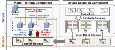
Figure 1: Architecture and Workflow of FedCat Framework

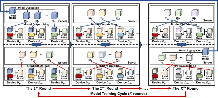
Figure 2: Workflow of Device Concatenation-based Model Training

3.1 FedCat Implementation

Figure 1 shows an overview of the architecture and workflow of our FedCat approach. The framework consists of two components, i.e., the device selection component and the model training component. At the beginning of each training round, the device selection component randomly groups all the devices and conducts device selection from these groups. The model training component performs the local training on selected devices, where each model training cycle includes multiple training rounds. Here, a model training cycle consists of three stages, i.e., model duplication, training iteration, and model aggregation. The model duplication stage generates $K$ copies of the global model. The training iteration stage dispatches the copies to the selected devices for local training and updates the copies after gradient collection. At the end of each cycle, the server obtains a new global model by aggregating all the latest model copies.

Algorithm 1 Workflow of FedCat

Input: i) $rnd$, the total number of training rounds; ii) $S_{dev}$, the set of devices; iii) $K$, the number of participating devices in a training round
Output: i) $m_{glb}$, the trained global model
FedCat($rnd$,$S_{dev}$,$K$)

1:  $r\leftarrow 0$, $N\leftarrow len(S_{dev})$ 

2:  $M_{dev}\leftarrow Map[N][K]$, $L_{m}\leftarrow[]$ 

3:  Initialize model $m_{glb}$ 

4:  for $r=0,1,...,rnd-1$ do

5:     if $r\%(\lambda\times K)=0$ then

6:        Randomly divide $S_{dev}$ into $\mathcal{G}=\{\mathcal{G}_{1},...,\mathcal{G}_{K}$} 

7:     end if

8:     $L_{dev},M_{dev}\leftarrow DevSelect(\mathcal{G},M_{dev},r,K)$ 

9:     if $r\%K=0$ then

10:        Duplicate $K$ copies of $m_{glb}$ in $L_{m}$ 

11:     end if

12:     offset$\leftarrow r\%K$ 

13:     $L_{m}\leftarrow TrainIter(L_{dev},L_{m},$offset$)$ 

14:     if $r\%K=K-1$ then

15:        $m_{glb}\leftarrow Aggregation(L_{m})$ 

16:     end if

17:     $r\leftarrow r+1$ 

18:  end for

19:  return $m_{glb}$ 

Algorithm 1 presents the workflow of FedCat in detail. Lines 5-17 show the details of one FL round for FedCat including both device selection and model training processes. Lines 5-8 present the device selection process in each training round, where we randomly divide all the devices into $K$ groups and select one device from each group for local training. The function $DevSelect$ denotes the device selection strategy which is implemented in Algorithm 3. $L_{dev}$ is the list of selected devices and $M_{dev}$ is a map that records the participation per device. Note that we regroup devices in every $\lambda\times k$ rounds, where $\lambda$ is a hyperparameter that controls the frequency of device grouping. Lines 9-16 denote the model training process. Line 10 generates $K$ copies of the global model $m_{glb}$ in every $K$ rounds. In Line 13, $L_{m}$ is a list of 2-tuples in the form of $\langle m,d\rangle$, where $m$ indicates a model with $d$ accumulated training data. The function $TrainIter$ denotes one training iteration stage, which dispatches models in $L_{m}$ to selected devices in $L_{dev}$ and updates $L_{m}$ after collecting the trained local models. The details of $TrainIter$ are shown in Algorithm 2. Note that we use a variable (i.e., offset) of integer type to guide the model dispatching and gradient collection processes. Line 15 denotes the model aggregation stage that aggregates models according to the size of accumulated training data. We aggregate models in every $K$ rounds and the $Aggregation$ function is defined as

$$Aggregation(L_{m})= \frac{\sum_{i=1}^{K}d_{i}\cdot m_{i}}{\sum_{j=1}^{K}d_{j}},$$ (3)

where $m_{i}$ indicates the $i^{th}$ model in $L_{m}$ and $d_{i}$ denotes the size of the training data set used by $m_{i}$.

3.2 Device Concatenation-Based Model Training

Figure 2 shows the workflow of our device concatenation-based model training strategy. Each model training cycle contains $K$ model training rounds, where $K$ equals the number of selected devices in each round. The server duplicates $k$ copies of the global model in the first round of each model training cycle. After that, the server conducts $K$ training iterations, where each training iteration involves three steps:

• Step 1: The server dispatches all the model copies to selected devices. In our approach, we dispatch the $i^{th}$ model copy to the $((i+j-2)\%K+1)^{th}$ selected device in the $j^{th}$ round of a model training cycle. For example, in Figure 2, $m_{1}$ is dispatched to the second device $D_{\mathcal{G}_{2}}$ in the second round.

• Step 2: The selected devices train received models using their local data and upload their gradients after local training finish.

• Step 3: The server updates all the model copies with the corresponding gradients. As an example shown in Figure 2, in the second round, the server updates $m_{1}$ using the gradient uploaded by the second device $D_{\mathcal{G}_{2}}$.

Note that, in the last round (i.e., the $K^{th}$ round) of each model training cycle, the aggregation stage aggregates all the updated model copies.

Algorithm 2 Training Iteration

Input: i) $L_{dev}$, the list of selected devices; ii) $L_{m}$, the initial list of models with the sizes of their accumulated training data; iii) offset, device index offset for model dispatching
Output: $L_{m}$, an updated list of models with the sizes of their accumulated training data
TrainIter($L_{dev}$,$L_{m}$,offset)

1:  $K\leftarrow len(L_{m})$ 

2:  for $\langle m_{i},d_{i}\rangle$ in $L_{m}$ do

3:     $tag\leftarrow($offset$+i)\%K$ 

4:     $dev\leftarrow L_{dev}[tag]$ 

5:     $Dispatch(tag,m_{i},dev)$ 

6:  end for

7:  $L_{\nabla},L_{d}\leftarrow GradientCollect()$

8:  for each $\langle m_{i},d_{i}\rangle$ in $L_{m}$ do

9:     $tag\leftarrow($offset$+i)\%K$ 

10:     $m_{i}\leftarrow m_{i}+L_{\nabla}[tag]$ 

11:     $d_{i}\leftarrow d_{i}+L_{d}[tag]$  

12:  end for

13:  return $L_{m}$ 

Algorithm 2 shows the details of a training iteration. Lines 2-6 denote the model dispatching process, where we use offset to guide the model dispatching. The function $GradientCollect$ in Line 7 collects the uploaded gradients and the sizes of training data from selected devices. The list $L_{\nabla}$ stores the uploaded gradients and the list $L_{d}$ stores the sizes of local training datasets. Lines 8-12 denote the model updating process. Line 10 updates the $i^{th}$ model copy $m_{i}$ using the corresponding uploaded gradient. Line 11 updates the size of accumulated training data by adding the size of training data to it.

3.3 Grouping- and Count-Based Device Selection

To encourage more devices to participate in model training and avoid training one model with the same device multiple times in one training cycle, we propose a grouping- and count-based device selection strategy. We define a count table $M_{dev}$ to count the device participation in each round of the training cycle. Since each training cycle contains $K$ rounds, the count table is a matrix of size $N\times K$ where $N$ is the number of devices. We use MBIE-EB Bellemare et al. (2016) to measure the weight of candidate devices, which is defined as:

$$w_{dev}=\frac{1}{\sqrt{M_{dev}[dev][{\it offset}]}}.$$ (4)

We use $\epsilon$-greedy policy to select a device. It means that we select the device with the maximum weight having a probability of $\epsilon$ and select the device according to the following probability distribution with a probability of $1-\epsilon$:

$$P(dev)=\frac{w_{dev}}{\sum_{dev\in\mathcal{G}_{i}}w_{dev}}.$$ (5)

Algorithm 3 details our grouping- and count-based device selection strategy. $\mathcal{G}$ is the set of device groups. $L_{dev}$ is a list to store selected devices. The table $M_{dev}$ is our defined count table. Lines 2-10 show the device selection details. In Line 4, we select a device from group $\mathcal{G}_{i}$ according to the policy $\pi_{\theta}$ based on the distribution defined in equation 5. Line 6 selects the device with the maximum weight from group $\mathcal{G}_{i}$. Line 9 updates count table after device selection.

Algorithm 3 Device Selection Strategy

Input: i) $rnd$, the number of FL training round; ii) $S_{dev}$, the set of devices; iii) $K$, the number of devices which participate training in a round; iv) $\mathcal{G}$, the set of device groups
Output: i) $L_{dev}$, a list of selected devices; ii) $M_{dev}$, an updated count map
DevSelect($S_{dev}$,$M_{dev}$,$r$,$K$)

1:  $L_{dev}\leftarrow[]$ 

2:  for each group $\mathcal{G}_{i}$ in $\mathcal{G}=\{\mathcal{G}_{1},...\mathcal{G}_{K}$} do

3:     if $random(0,1.0)>\epsilon$ then

4:        select $dev\sim\pi_{\theta}(\mathcal{G}_{i},M_{dev})$ 

5:     else

6:        $dev\leftarrow\arg\max\limits_{dev\in\mathcal{G}_{i}}{w_{dev}}$  

7:     end if

8:     $L_{dev}.append(dev)$ 

9:     $M_{dev}[dev][r\%K]\leftarrow M_{dev}[dev][r\%K]+1$ 

10:  end for

11:  return $L_{dev}$, $M_{dev}$ 

Dataset	Heterogeneity	Test Accuracy (%)
	Settings	FedAvg	FedProx	SCAFFOLD	FedGen	CluSamp	FedCat (Ours)
MNIST	$\alpha=0.1$	$99.04$	$99.02$	$98.92$	$99.18$	$98.98$	${\bf 99.21}$
	$\alpha=0.5$	$99.31$	$99.27$	$99.28$	$99.41$	$99.27$	${\bf 99.42}$
	$\alpha=1.0$	$99.37$	$99.30$	$99.32$	$99.37$	$99.33$	${\bf 99.4}$
CIFAR-10	$\alpha=0.1$	$51.01$	$51.85$	$52.81$	$51.42$	$51.60$	${\bf 56.16}$
	$\alpha=0.5$	$54.32$	$54.99$	$56.09$	$53.4$	$55.16$	${\bf 57.89}$
	$\alpha=1.0$	$55.69$	$55.58$	$58.13$	$56.34$	$56.82$	${\bf 61.45}$
CIFAR-100	$\alpha=0.1$	$29.95$	$29.76$	$31.77$	$29.01$	$29.86$	${\bf 33.82}$
	$\alpha=0.5$	$31.03$	$32.97$	$34.06$	$30.31$	$33.96$	${\bf 36.85}$
	$\alpha=1.0$	$33.05$	$33.74$	$35.81$	$31.88$	$33.08$	${\bf 37.26}$
FEMNIST	-	$82.32$	$82.61$	$81.88$	$82.86$	$81.68$	${\bf 83.94}$

Table 1: Test accuracy on various partitions of MNIST, CIFAR10, CIFAR100, and FEMNIST

3.4 Convergence Analysis

We provide insights into the convergence analysis for FedCat based on the following assumptions about the loss functions of local devices.

Assumption 3.1.

For $i=1,2,\cdots,N$, $f_{i}$ is L-smooth satisfying $||\nabla f_{i}(x)-\nabla f_{i}(y)||\leq l||x-y||$.

Assumption 3.2.

For $i=1,2,\cdots,N$, $f_{i}$ is $\mu$-convex satisfying $||\nabla f_{i}(x)-\nabla f_{i}(y)||\geq\mu||x-y||$, where $\mu\geq 0$.

Assumption 3.3.

The variance of stochastic gradients is upper bounded by $\beta^{2}$ and the expectation of squared norm of stochastic gradients is upper bounded by $G^{2}$, i.e., $\mathbb{E}||\nabla f_{k}(w;\xi)-\nabla f_{k}(w)||^{2}\leq\beta^{2}$, $\mathbb{E}||\nabla f_{k}(w;\xi)||^{2}\leq G^{2}$, where $\xi$ is a data batch of the $k^{th}$ device in the $t^{th}$ iteration.

In the case where all the devices participate in every round of local training, inspired by the work in Li et al. (2020b), we can derive Theorem 3.1:

Theorem 3.1.

Let Assumption 3.1, Assumption 3.2, Assumption 3.3 hold. After the aggregation in each round, we have

$$\begin{split}\mathbb{E}||F(\overline{w}_{t})||-F^{\star}\leq\frac{L}{\mu(\gamma+t-1)}(\frac{2B}{\mu}+\frac{\mu\gamma}{2}\mathbb{E}||\overline{w}_{1}-w^{\star}||^{2})\end{split},$$

where $B=\frac{1}{N}\beta^{2}+6L\Gamma+8(KE-1)^{2}G^{2}.$

Theorem 3.1 indicates that the difference between the current loss $F(\overline{w}_{t})$ and the optimal loss $F^{\star}$ is inversely related to $t$. From Theorem 3.1, we can find that the convergence rate of FedCat is consistent with that of FedAvg, which is analyzed in Li et al. (2020b). Please refer to Appendix A for more details of the proof.

4 Experimental Results

To evaluate the performance of our FedCat method, we compared both the model accuracy and convergence of FedCat with five baselines using four well-known benchmarks. Moreover, we designed ablation studies to demonstrate the effectiveness of our proposed device concatenation-based training and device selection strategies.

(a) CIFAR-10 with $\alpha=0.1$

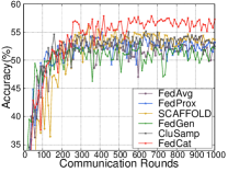
(b) CIFAR-10 with $\alpha=0.5$

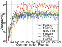
(c) CIFAR-10 with $\alpha=1.0$

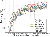
(d) FEMNIST

Figure 3: Comparison results between of our FedCat approach and five baseline methods

4.1 Experimental Settings

We implemented our approach on top of a cloud server and a large set of local devices. Since it is difficult for all the devices to participate in the training process simultaneously in practice, by default we assumed that there are only 10% of the overall local devices selected to participate in each round of model training. We used the SGD optimizer with a learning rate 0.01, where the SGD momentum is 0.9 for all the methods. For each device, we set the batch size of its local training to 50, and performed five epochs for each local training. We tested the accuracy of the global model in every ten rounds, where each round involves a pair of model upload and dispatch operations. We performed experiments on a workstation with Intel i9-10900k CPU, 32GB memory, NVIDIA GeForce RTX 3080 GPU, and Ubuntu operating system (version 18.04).

Dataset and Model Settings: Our experiments were conducted on four well-known datasets, i.e., MNIST, CIFAR-10, CIFAR-100 TorchvisionData (2019), and FEMNIST Caldas et al. (2018). For the first three datasets, we assumed that there are 100 devices got involved in FL. For FEMNIST, we considered a non-IID scenario with 180 devices, where each consists of more than 100 local samples. For MNIST and CIFAR-10, we adopted the same CNN models as the ones used in McMahan et al. (2017). We use the CNN model of MNIST for FEMNIST with slight modification. Since the number of categories of FEMNIST is 62, we changed the output size of MNIST CNN model to 62 for FEMNIST. For CIFAR-100, we modified the output size of the CIFAR-10 CNN model to 20, since there are 20 categories of coarse-grained labels in CIFAR-100.

Data Heterogeneity Settings: In the experiment, we adopted the Dirichlet distribution Hsu et al. (2019) to control the heterogeneity of device data for MNIST, CIFAR-10, and CIFAR-100. Here, we use the notation $Dir(\alpha)$ to denote different Dirichlet distributions controlled by $\alpha$, where a smaller value of $\alpha$ indicates higher data heterogeneity. For each one of datasets MNIST, CIFAR-10, and CIFAR-100, we investigated three cases following different Dirichlet distributions with $\alpha=0.1$, $0.5$, and $1.0$, respectively. Note that, different from the other three datasets, the raw data of FEMNIST is naturally non-IID distributed considering various kinds of imbalances including class imbalance, data imbalance, and data heterogeneity.

Baseline Methods: To fairly evaluate the performance of our approach, we compared the model accuracy of FedCat with five baseline methods, i.e., FedAvg McMahan et al. (2017), FedProx Li et al. (2020a), SCAFFOLD Karimireddy et al. (2019), FedGen Zhu et al. (2021), and CluSamp Fraboni et al. (2021). FedAvg is the most classical FL method and the other four methods are the state-of-the-art representatives of the three kinds of FL methods introduced in Section 2. FedProx and SCAFFOLD are global control variable-based methods. FedGen is a KD-based approach, and CluSamp is a device grouping-based method. Note that, FedProx uses a hyperparameter $\mu$ to control the weight of its proximal term. When using FedProx, we only considered four values for $\mu$ defined in the set {0.001,0.01,0.1,1}. We explored the best values of $\mu$ for MNIST, CIFAR-10, CIFAR-100, and FEMNIST, which 0.1, 0.01, 0.001, and 0.1, respectively. For FedGen, we used the same global generator training setting as Zhu et al. (2021) for the server. For CluSamp, we clustered devices based on the similarity of model gradients in the same way as Fraboni et al. (2021).

4.2 Performance Comparison

To evaluate the performance of our approach, we compared our approach with five baselines on four datasets. Due to the space limitation, here we only present the comparison results for CIFAR-10. All the supplementary experimental results are included in Appendix B.

Comparison of Accuracy: Table 1 presents the performance comparison results between our FedCat and the five baseline methods in terms of test accuracy. Note that the second column shows the values of the hyperparameter $\alpha$ that control the data heterogeneity based on the Dirichlet distribution. From Table 1, we can observe that compared with the five baseline methods, our approach can archive the highest accuracy on all the scenarios with different data heterogeneity settings. As an example of CIFAR-10, when $\alpha$ equals 0.1, our FedCat outperforms FedAvg, FedProx, SCAFFOLD, FedGen, and CluSamp by 5.15%, 4.31%, 3.35%, 4.74%, and 4.56%, respectively. Note that, our approach can achieve better improvements on the datasets CIFAR-10 and CIFAR-100 than the datasets MINST and FEMNIST. This is because the datasets MINST and FEMNIST are much simpler than the datasets CIFAR-10 and CIFAR-100, where all the FL methods in the table can achieve almost the best test accuracy.

Figure 3 presents the model accuracy trends of all the investigated FL methods considering different data heterogeneity settings for datasets CIFAR-10 and FEMNIST. Note that here one communication round indicates one interaction between the server and devices including both the gradient upload and model dispatch operations. From this figure, we can find that FedCat cannot only achieve the highest accuracy, but also converge more quickly than the other methods to their highest accuracy.

Analysis of Communication Overhead: Similar to FedAvg, FedProx, and CluSamp, in one round of FL, the communication overhead of FedCat only involves the network traffic generated by both model dispatching and gradient uploading operations. Due to the usage of extra global control variables, SCAFFOLD needs twice as much network traffic as FedCat. For FedGen, the communication overhead is more than FedAvg, since it needs to dispatch an additional built-in generator with a non-negligible size compared to the model itself. In a nutshell, the communication overhead required by FedCat is the least among all the six FL methods.

4.3 Ablation Study

We conducted ablation studies to demonstrate the effectiveness of both of our proposed device concatenation-based model training and grouping- and count-based device selection. We use the notations “FedCat w/ GC” to denote the FedCat variant implemented with only grouping- and count-based device selection strategy and “FedCat w/ DC” to indicate the FedCat variant implemented with only device concatenation-based model training. For FedCat w/ GC, we aggregate models in every FL round. For FedCat w/ DC, we randomly select devices without grouping. Note that, we consider the FedAvg in the ablation studies, since FedAvg is a specific FedCat variant without considering device concatenation-based model training or grouping- and count-based device selection.

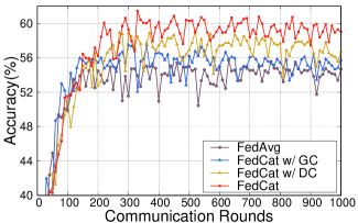
Figure 4: Ablation studies of model accuracy

Due to the space limitation, Figure 4 only shows the ablation study results on CIFAR-10 with $\alpha=1.0$. We can observe that FedCat can achieve the highest model accuracy, while both FedCat w/ GC and FedCat w/ DC have better model accuracy than FedAvg. Please refer to Appendix B for the ablation study results of the other datasets.

5 Conclusion

Although Federated Learning (FL) approaches are promising to enable collaborative learning for a large set of involved devices without causing data privacy leakage, they still suffer from the problem of model inaccuracy in various non-IID scenarios. This is because the local models of traditional FL methods are trained on individual devices with insufficient and skewed training data, which can easily lead to weight divergence during the training of local models. To address this problem, we proposed a novel FL method named FedCat, which allows local models to traverse through a series of selected devices during the local training by using our proposed count-based device selection strategy and device concatenation-based local training method. Due to the large size of training data contained by logically concatenated devices, FedCat can effectively mitigate the problem of model weight divergence during the local training process, thus improving the overall FL performance for non-IID scenarios. Comprehensive experimental results on four well-known benchmarks show the effectiveness of our approach.

Appendix A Proof of Convergence Analysis

In our scenario, all devices have the same weight. $t$ exhibits the $t^{th}$ SGD iteration on the local device. $v$ is the intermediate variable that represents the result of SGD update after exactly one iteration. The update of FedCat is as follows:

$$v_{t+1}^{k}=w_{t}^{k}-\eta_{t}\nabla f_{k}(w_{t}^{k},\xi_{t}^{k}),$$

where $w_{t}^{k}$ represents the model of the $k^{th}$ device in the $t^{th}$ iteration.

$$w_{t+1}^{k}=\left\{\begin{array}[]{rl}v_{t+1}^{k},&if\quad E\nmid t+1\\ v_{t+1}^{i}(i\neq k),&if\quad E\mid t+1,KE\nmid t+1\\ \frac{1}{N}\sum_{i=1}^{N}v_{t+1}^{i},&if\quad KE\mid t+1\\ \end{array}\right.$$

Similar to Stich [2019], we define two variables $\overline{v}_{t}$ and $\overline{w}_{t}$:

$$\begin{split}\overline{v}_{t}=\frac{1}{N}\sum_{k=1}^{N}v_{t}^{k},\overline{w}_{t}=\frac{1}{N}\sum_{k=1}^{N}w_{t}^{k}.\end{split}$$

Here we explain why $\overline{w}_{t}=\overline{v}_{t}$. We consider the following three cases:

• If $E\nmid t+1$, notice that $w_{t+1}^{k}=v_{t+1}^{k}$, then $\overline{w}_{t}=\overline{v}_{t}$.

• If $E\mid t+1$ and $KE\nmid t+1$, $\overline{w}_{t+1}=\frac{1}{N}\sum_{k=1}^{N}w_{t+1}^{k}=\frac{1}{N}\sum_{k=1}^{N}v_{t+1}^{k}=\overline{v}_{t+1}$.

• If $KE\mid t+1$, $w_{t+1}^{1}=w_{t+1}^{2}=\cdots=w_{t+1}^{N}=\frac{1}{N}\sum_{k=1}^{N}w_{t+1}^{k}=\overline{w}_{t+1}=\frac{1}{N}\sum_{k=1}^{N}v_{t+1}^{k}=\overline{v}_{t+1}$.

Inspired by Li et al. [2020b], we make the following definition: $g_{t}=\sum_{k=1}^{N}p_{k}\nabla f_{k}(w_{t}^{k};\xi_{t}^{k})$. $\overline{g}_{t}=\sum_{k=1}^{N}p_{k}\nabla f_{k}(w_{t}^{k})$. $\mathbb{E}[g_{t}]=\overline{g}_{t}$. $\overline{v}_{t+1}=\overline{w}_{t}-\eta_{t}g_{t}$.

Lemma A.1.

According to Lemma 1 in Li et al. [2020b],

$$\begin{split}\mathbb{E}||\overline{v}_{t+1}-w^{\star}||&\leq(1-\eta_{t}\mu)\mathbb{E}||\overline{w}_{t}-w^{\star}||^{2}+\eta_{t}^{2}\mathbb{E}||g_{t}-\overline{g}_{t}||^{2}\\ &+6L\eta_{t}^{2}\Gamma+\frac{2}{N}\mathbb{E}\sum_{k=1}^{N}||\overline{w}_{t}-w_{t}^{k}||^{2}\end{split}$$

Lemma A.2.

The variance of $g_{t}$ is upper bounded, where all devices have the same aggregation weight $\frac{1}{N}$:

$$\begin{split}\mathbb{E}||g_{t}-\overline{g}_{t}||^{2}\leq\frac{1}{N^{2}}\sum_{k=1}^{N}\beta^{2}\end{split}$$

Proof.

For the independent random variables, the variance of their sum is equivalent to the sum of their variance.

$$\begin{split}\mathbb{E}||\sum_{k=1}^{N}(X_{k}-\mathbb{E}X_{k})||^{2}=\sum_{k=1}^{N}\mathbb{E}||X_{k}-\mathbb{E}X_{k}||^{2}\end{split}$$

Here we use $X_{k}=\frac{1}{N}\nabla f_{k}(w_{t}^{k};\xi_{t}^{k})$, $\mathbb{E}X_{k}=\frac{1}{N}\nabla f_{k}(w_{t}^{k})$.

$$\begin{split}\mathbb{E}||g_{t}-\overline{g}_{t}||^{2}&=\mathbb{E}||\frac{1}{N}\sum_{k=1}^{N}(\nabla f_{k}(w_{t}^{k},\xi_{t}^{k})-\nabla f_{k}(w_{t}^{k}))||^{2}\\ &=\sum_{k=1}^{N}\frac{1}{N^{2}}\mathbb{E}||\nabla f_{k}(w_{t}^{k},\xi_{t}^{k})-\nabla f_{k}(w_{t}^{k}))||^{2}\\ &\leq\frac{1}{N^{2}}\sum_{k=1}^{N}\beta^{2}\\ \end{split}$$

∎

Lemma A.3.

Within our configuration, the aggregation occurs every $KE$ iterations. For arbitrary t, there always exists $t_{0}\leq t$ while $t_{0}$ is the nearest aggregation moment to $t$. As a result, $t-t_{0}\leq KE-1$ holds. Given the constraint on learning rate from Li et al. [2020b], we know that $\eta_{t}\leq\eta_{t_{0}}\leq 2\eta_{t}$. It follows that

$$\begin{split}\mathbb{E}\sum_{k=1}^{N}\frac{1}{N}||\overline{w}_{t}-w_{t}^{k}||^{2}\leq 4\eta_{t}^{2}(KE-1)^{2}G^{2}.\end{split}$$

Proof.

Let m = $\lfloor\frac{t-t_{0}}{E}\rfloor$ and the concatenated clients set $A=\{a_{1},a_{2},...,k\}$.

$$\begin{split}||w_{t}^{k}-\overline{w}_{t_{0}}||^{2}=&||\sum_{t=t_{0}}^{t_{0}+E-1}\eta_{t}\nabla f_{a_{1}}(w_{t}^{a_{1}};\xi_{t}^{a_{1}})+\\ &\sum_{t=t_{0}+E}^{t_{0}+2E-1}\eta_{t}\nabla f_{a_{2}}(w_{t}^{a_{2}};\xi_{t}^{a_{2}})+\cdots+\\ &\sum_{t=t_{0}+mE}^{t}\eta_{t}\nabla f_{k}(w_{t}^{k};\xi_{t}^{k})||^{2}\\ &\leq(t-t_{0})\sum_{t=t_{0}}^{t-1}\eta_{t}^{2}G^{2}\\ &\leq(KE-1)\sum_{t=t_{0}}^{t-1}\eta_{t}^{2}G^{2}\\ \end{split}$$

where the first inequality is accomplished via adopting AM-GM inequality.

$$\begin{split}\mathbb{E}\sum_{k=1}^{N}\frac{1}{N}||\overline{w}_{t}-w_{t}^{k}||^{2}&=\mathbb{E}\sum_{k=1}^{N}\frac{1}{N}||(w_{t}^{k}-\overline{w}_{t_{0}})-(\overline{w}_{t}-\overline{w}_{t_{0}})||^{2}\\ &\leq\mathbb{E}\sum_{k=1}^{N}\frac{1}{N}||w_{t}^{k}-\overline{w}_{t_{0}}||^{2}\\ &\leq\sum_{k=1}^{N}\frac{1}{N}\mathbb{E}\sum_{t=t_{0}}^{t-1}(KE-1)\eta_{t_{0}}^{2}||\nabla f_{k}(w_{t}^{k},\xi_{t}^{k})||^{2}\\ &\leq\sum_{k=1}^{N}\frac{1}{N}\mathbb{E}\sum_{t=t_{0}}^{t-1}(KE-1)\eta_{t_{0}}^{2}G^{2}\\ &\leq 4\eta_{t}^{2}(KE-1)^{2}G^{2}.\end{split}$$

∎

From Lemma A.1, Lemma A.2, and Lemma A.3, we can derive Theorem 3.1:

$$\begin{split}\mathbb{E}||F(\overline{w}_{t})||-F^{\star}\leq\frac{L}{\mu(\gamma+t-1)}(\frac{2B}{\mu}+\frac{\mu\gamma}{2}\mathbb{E}||\overline{w}_{1}-w^{\star}||^{2})\end{split},$$

where $B=\frac{1}{N}\beta^{2}+6L\Gamma+8(KE-1)^{2}G^{2}.$

Dataset	Heterogeneity	Test Accuracy (%)
	Settings	FedAvg	FedProx	SCAFFOLD	FedGen	CluSamp	FedCat (Ours)
MNIST	$\alpha=0.1$	$99.04$	$99.02$	$98.92$	$99.18$	$98.98$	${\bf 99.21}$
	$\alpha=0.5$	$99.31$	$99.27$	$99.28$	$99.41$	$99.27$	${\bf 99.42}$
	$\alpha=1.0$	$99.37$	$99.30$	$99.32$	$99.37$	$99.33$	${\bf 99.4}$
CIFAR-10	$\alpha=0.1$	$51.01$	$51.85$	$52.81$	$51.42$	$51.60$	${\bf 56.16}$
	$\alpha=0.5$	$54.32$	$54.99$	$56.09$	$53.4$	$55.16$	${\bf 57.89}$
	$\alpha=1.0$	$55.69$	$55.58$	$58.13$	$56.34$	$56.82$	${\bf 61.45}$
CIFAR-100	$\alpha=0.1$	$29.95$	$29.76$	$31.77$	$29.01$	$29.86$	${\bf 33.82}$
	$\alpha=0.5$	$31.03$	$32.97$	$34.06$	$30.31$	$33.96$	${\bf 36.85}$
	$\alpha=1.0$	$33.05$	$33.74$	$35.81$	$31.88$	$33.08$	${\bf 37.26}$
FEMNIST	-	$82.32$	$82.61$	$81.88$	$82.86$	$81.68$	${\bf 83.94}$

Table 2: Test accuracy on various data distributions of MNIST, CIFAR10, CIFAR100, and FEMNIST

Appendix B Supplementary Experimental Results for Accuracy Comparison and Ablation Study

B.0.1 Experimental Results for Accuracy Comparison

Table 2 presents test accuracy for our proposed FedCat and five baselines in 10 scenarios. Figure 5 presents the trend of accuracy of our approach and baselines.

B.0.2 Experimental Results of Ablation Studies

Table 3 presents the test accuracy of our ablation studies. Figure 6 presents the trend of accuracy of our ablation studies on CIFAR-10 and CIFAR-100.

Dataset	Heterogeneity	Test Accuracy (%)
	Settings	FedAvg	FedCat	FedCat	FedCat
			w/ GC	w/ DC
CIFAR-10	$\alpha=0.1$	$51.01$	$51.02$	$55.06$	${\bf 56.16}$
	$\alpha=0.5$	$54.32$	$57.20$	$57.51$	${\bf 57.89}$
	$\alpha=1.0$	$55.69$	$57.54$	$59.12$	${\bf 61.45}$
CIFAR-100	$\alpha=0.1$	$29.95$	$31.41$	$31.82$	${\bf 33.82}$
	$\alpha=0.5$	$31.03$	$32.28$	$35.62$	${\bf 36.85}$
	$\alpha=1.0$	$33.05$	$33.28$	$36.78$	${\bf 37.26}$

Table 3: Test accuracy of ablation studies

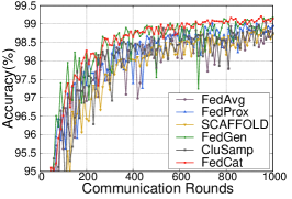
(a) MNIST $\alpha=0.1$

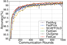
(b) MNIST $\alpha=0.5$

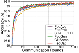
(c) MNIST $\alpha=1.0$

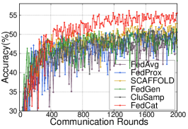
(d) CIFAR-10 $\alpha=0.1$

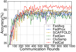
(e) CIFAR-10 $\alpha=0.5$

(f) CIFAR-10 $\alpha=1.0$

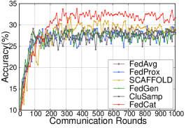
(g) CIFAR-100 $\alpha=0.1$

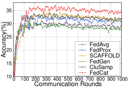
(h) CIFAR-100 $\alpha=0.5$

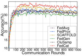
(i) CIFAR-100 $\alpha=1.0$

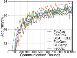
(j) FEMNIST

Figure 5: Model accuracy comparison between our approach and baselines

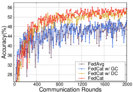
(a) CIFAR-10 $\alpha=0.1$

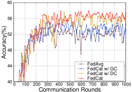
(b) CIFAR-10 $\alpha=0.5$

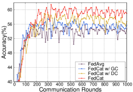
(c) CIFAR-10 $\alpha=1.0$

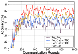
(d) CIFAR-100 $\alpha=0.1$

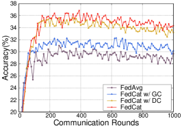
(e) CIFAR-100 $\alpha=0.5$

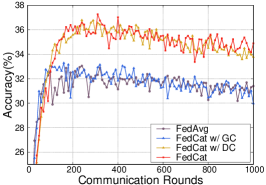
(f) CIFAR-100 $\alpha=1.0$

Figure 6: Ablation studies of model accuracy

References

- Bellemare et al. [2016] M. Bellemare, S. Srinivasan, G. Ostrovski, T. Schaul, D. Saxton, and R. Munos. Unifying count-based exploration and intrinsic motivation. In Advances in Neural Information Processing Systems (NeurIPS), pages 1471–1479, 2016.
- Caldas et al. [2018] S. Caldas, P. Wu, T. Li, J. Konecny, H. McMahan, V. Smith, and A. Talwalkar. LEAF: A benchmark for federated settings. CoRR, abs/1812.01097, 2018.
- Chen et al. [2020] C. Chen, Z. Chen, Y. Zhou, and B. Kailkhura. Fedcluster: Boosting the convergence of federated learning via cluster-cycling. In Proceedings of International Conference on Big Data (BigData), pages 5017–5026, 2020.
- et al. [2021] P. Kairouz et al. Advances and open problems in federated learning. Found. Trends Mach. Learn., 14(1-2):1–210, 2021.
- Fraboni et al. [2021] Y. Fraboni, R. Vidal, L. Kameni, and M. Lorenzi. Clustered sampling: low-variance and improved representativity for clients selection in federated learning. In Proceedings of International Conference on Machine Learning (ICML), volume 139, pages 3407–3416, 2021.
- Hsu et al. [2019] T. Hsu, H. Qi, and M. Brown. Measuring the effects of non-identical data distribution for federated visual classification. CoRR, abs/1909.06335, 2019.
- Hu et al. [2021] R. Hu, Y. Gong, and Y. Guo. Federated learning with sparsification-amplified privacy and adaptive optimization. In Proceedings of International Joint Conference on Artificial Intelligence (IJCAI), pages 1463–1469, 2021.
- Huang et al. [2021a] H. Huang, F. Shang, Y. Liu, and H. Liu. Behavior mimics distribution: combining individual and group behaviors for federated learning. In Proceedings of International Joint Conference on Artificial Intelligence (IJCAI), pages 2556–2562, 2021.
- Huang et al. [2021b] Y. Huang, L. Chu, Z. Zhou, L. Wang, J. Liu, J. Pei, and Y. Zhang. Personalized cross-silo federated learning on non-iid data. In Proceedings of Conference on Artificial Intelligence (AAAI), pages 7865–7873, 2021.
- Karimireddy et al. [2019] S. Karimireddy, S. Kale, M. Mohri, S. Reddi, S. Stich, and A. Suresh. SCAFFOLD: stochastic controlled averaging for on-device federated learning. CoRR, abs/1910.06378, 2019.
- Li and Wang [2019] D. Li and J. Wang. Fedmd: Heterogenous federated learning via model distillation. CoRR, abs/1910.03581, 2019.
- Li et al. [2020a] T. Li, A. Sahu, M. Zaheer, M. Sanjabi, A. Talwalkar, and V. Smith. Federated optimization in heterogeneous networks. In Proceedings of Machine Learning and Systems (MLSys), 2020.
- Li et al. [2020b] X. Li, K. Huang, W. Yang, S. Wang, and Z. Zhang. On the convergence of fedavg on non-iid data. In Proceedings of International Conference on Learning Representations (ICLR), 2020.
- Li et al. [2021] Q. Li, B. He, and D. Song. Practical one-shot federated learning for cross-silo setting. In Proceedings of International Joint Conference on Artificial Intelligence (IJCAI), pages 1484–1490, 2021.
- Lin et al. [2020] T. Lin, L. Kong, S. Stich, and M. Jaggi. Ensemble distillation for robust model fusion in federated learning. In Proceedings of Annual Conference on Neural Information Processing Systems 2020 (NeurIPS), 2020.
- McMahan et al. [2017] B. McMahan, E. Moore, D. Ramage, S. Hampson, and B. Arcas. Communication-efficient learning of deep networks from decentralized data. In Proceedings of International Conference on Artificial Intelligence and Statistics (AISTATS), volume 54, pages 1273–1282, 2017.
- Stich [2019] Sebastian U. Stich. Local SGD converges fast and communicates little. In Proceedings of International Conference on Learning Representations (ICLR), 2019.
- Sun et al. [2021] L. Sun, J. Qian, and X. Chen. LDP-FL: practical private aggregation in federated learning with local differential privacy. In Proceedings of International Joint Conference on Artificial Intelligence (IJCAI), pages 1571–1578, 2021.
- TorchvisionData [2019] TorchvisionData. Dataset of mnist, fashion-mnist, cifar-10 and cifar-100. Website, 2019. https://pytorch.org/docs/stable/torchvision/datasets.html.
- Wang et al. [2020] H. Wang, Z. Kaplan, D. Niu, and B. Li. Optimizing federated learning on non-iid data with reinforcement learning. In Proceedings of Conference on Computer Communications (INFOCOM), pages 1698–1707, 2020.
- Wang et al. [2021a] L. Wang, S. Xu, X. Wang, and Q. Zhu. Addressing class imbalance in federated learning. In Proceedings of Conference on Artificial Intelligence (AAAI), pages 10165–10173, 2021.
- Wang et al. [2021b] Z. Wang, X. Fan, J. Qi, C. Wen, C. Wang, and R. Yu. Federated learning with fair averaging. In Proceedings of International Joint Conference on Artificial Intelligence (IJCAI), pages 1615–1623, 2021.
- Xie et al. [2021] M. Xie, G. Long, T. Shen, T. Zhou, X. Wang, J. Jiang, and C. Zhang. Multi-center federated learning. CoRR, abs/2108.08647, 2021.
- Yang [2021] H. Yang. H-FL: A hierarchical communication efficient and privacy-protected architecture for federated learning. In Proceedings of International Joint Conference on Artificial Intelligence (IJCAI), pages 479–485, 2021.
- Zhu et al. [2021] Z. Zhu, J. Hong, and J. Zhou. Data-free knowledge distillation for heterogeneous federated learning. In Proceedings of International Conference on Machine Learning, ICML, volume 139, pages 12878–12889, 2021.