On the direct diagonalization method for a few particles trapped in harmonic potentials

Abstract

We describe a procedure to systematically improve direct diagonalization results for few-particle systems trapped in one-dimensional harmonic potentials interacting by contact interactions. We start from the two-body problem to define a renormalization method for the interparticle interactions. The procedure is benchmarked with state-of-the-art numerical results for three and four symmetric fermions.

I Introduction

Ultracold atomic gases laboratories provide versatile setups for the quantum simulation of a large number of phenomena in condensed matter and many-body quantum physics [1, 2]. These setups allow to study the onset of many-body quantum physics, in experiments where the systems can be made to transit from the few-body regime [3, 4, 5] into the many-body one, e.g. Bose-Einstein condensates [6].

Simultaneously, the theoretical and numerical efforts to understand the transition from the few- to the many-body problem have flourished in a number of well-consolidated techniques, such as Monte Carlo methods [7], tensor networks [8], mean-field approaches [6], coupled-cluster method  [9], direct diagonalization techniques [10, 11] and, more recently, machine learning ones [12]. All of them have their pros and cons, all of them bear inherent approximations which make them useful only in certain conditions, e.g. low dimensions, mild interaction regimes, few particles, etc.

In this work, we concentrate on direct diagonalization techniques mostly used for particles trapped in a 1D harmonic potential, e.g. [13, 14]. In this method the idea is simple, one needs to build the many-body Hamiltonian on a suitable basis and diagonalize it "exactly". The method does not provide exact results due to the truncations made on the Hilbert space. The usual procedure runs as follows: 1) fix the number of particles, $N$, to be either bosons or fermions, or mixtures. Then, 2) truncate the single-particle basis to $M$ modes, and 3) build the corresponding many-body basis performing a truncation on the total energy of the non-interacting many-body states [15].

This technique has been recently used to study small 1D bosonic mixtures [16, 17], fermionic systems [14], 2D bosonic systems with and without spin-orbit coupling [18, 19]. Even though direct diagonalization calculations are limited to a small number of particles, they offer several advantages compared to other approaches. First, they provide access to a large portion of the energy spectrum. In particular, they give the full solution of these states, including the eigenstates, excitation properties and spectral functions. In contrast, many approaches are restricted to a few ground-state properties. In addition, depending on the size of the truncated Hilbert space, direct diagonalization can be easily used to perform time-dependent calculations.

An issue that remains elusive concerns the way to perform extrapolations on the number of single-particle modes, $M$. This issue has been tackled in previous works, notably in Refs. [20, 21] and, specifically for harmonic traps, in Refs. [22, 23, 24]. These studies propose a heuristic scheme to perform the extrapolation of the results computed for a finite $M$ to the $M\to\infty$ limit. Other studies address this problem by describing an effective interaction, see Ref. [25, 26].

In this work, we describe a procedure to systematically perform the $M\to\infty$ limit of few-particle properties, e.g. we consider eigenenergies and density profiles. The procedure is benchmarked with state-of-the-art few-body calculations for $N=3$ and $N=4$ fermionic SU($N$) symmetric systems [27]. Our method shows an outstanding performance, providing results with less than $1\%$ of discrepancy with the exact ones for $N=3$ and $N=4$ particles with as few as 20 modes for interaction strengths $g$ in the whole $0\to\infty$ range.

Our work is organized as follows. In Sec. II we describe the Hamiltonian. Then, in Sec. III we revise the analytical solution of the two-particle case [28], which is then used in the extrapolation algorithm, described in this section. In Sec. IV we present how the procedure works for just two particles. In this case, the approach is exact and allows one to understand how to use it for more particles. In Sec. V we consider the few-particle scenario. There we compare with the exact results of Ref. [27] for the lower part of the energy spectrum obtained for three and four SU($N$) particles and we also report the energy predictions for five and six. We also discuss the correction on the single-particle density. Finally, in Sec. VI we present a summary and the main conclusions of our work.

II Model

Let us consider a system composed of a few particles, bosons or fermions, with a number of internal states, trapped in a one-dimensional harmonic oscillator (HO) potential. We assume that the interaction is properly described by a contact potential, as is the case for many ultracold atomic gases experiments, see for instance the reviews [2, 1]. In first quantization the Hamiltonian of the system for $N$ particles is

$$\hat{H}=\sum_{i=1}^{N}\left[-\frac{\hbar^{2}}{2m}\frac{\partial^{2}}{\partial x_{i}^{2}}+\frac{m\omega^{2}}{2}x_{i}^{2}\right]+\sum_{\alpha,\beta}g_{\alpha\beta}\sum^{N_{\alpha},N_{\beta}}_{i<j}\delta(x_{i}-x_{j})\,,$$ (1)

where $g_{\alpha\beta}$ is the interaction strength between the particles in internal states $\alpha$ and $\beta$, and $N_{\alpha}$ is the number of particles in the internal state $\alpha$.

By choosing the HO eigenfunctions as the single-particle basis, the HO part of the Hamiltonian (1) is diagonal with eigenvalues $\epsilon_{n_{i}}=(n_{i}+1/2)\hbar\omega$. $n_{i}$ is the index of the HO wavefunction of the state $|{i}\rangle$. This state has a spatial and a spin component: $|{i}\rangle=|{\Phi_{n_{i}}\chi_{s_{i}}}\rangle$, where $\Phi_{n_{i}}$ is the $n_{i}$-th HO wavefunction and $\chi_{s_{i}}$ is the internal state wavefunction of internal state $s_{i}$.

In the HO basis, the two-body matrix elements of the interacting part of the Hamiltonian (1) are expressed as [14],

$$v_{ij,kl}=g_{s_{i}s_{j}}\,\delta_{s_{i},s_{k}}\delta_{s_{j},s_{l}}\int dx\,\Phi_{n_{i}}(x)\Phi_{n_{j}}(x)\Phi_{n_{k}}(x)\Phi_{n_{l}}(x)\,,$$ (2)

where $\Phi_{n}(x)$ are the eigenfunctions of the HO Hamiltonian for the energy level $n$, which are real in one dimension. Note that we have used the orthogonality of the spin functions: $\langle\chi_{s_{i}}\chi_{s_{j}}|\chi_{s_{k}}\chi_{s_{l}}\rangle=\delta_{{s}_{i},{s}_{k}}\delta_{{s}_{j},{s}_{l}}$. We also stress that the interaction does not affect the spin of the particles. We numerically calculate the integral (2) using the procedure presented in Ref. [14].

The full Hamiltonian (1) in second quantization reads

$$\hat{H}=\sum_{i}\epsilon_{n_{i}}\hat{a}^{\dagger}_{i}\hat{a}_{i}+\frac{1}{2}\sum_{ijkl}v_{ij,kl}\hat{a}^{\dagger}_{i}\hat{a}^{\dagger}_{j}\hat{a}_{l}\hat{a}_{k}\,.$$ (3)

where $\hat{a}_{i}^{\dagger}$ ($\hat{a}_{i}$) creates (annihilates) a particle in the single-particle state $|{i}\rangle$.

III Correction of the truncated results

As explained above, using direct diagonalization techniques one numerically obtains the lower-energy eigenvalues and corresponding eigenstates in a truncated Hilbert space. Importantly, these techniques fall within the variational method, i.e. they do produce in all cases upper bounds to the corresponding exact eigenvalues. In practice, one has to truncate the single particle basis to a finite number of modes $M$ (for details see [14]). In this work, we additionally truncate the many-body basis up to a non-interacting energy $E_{\mathrm{max.}}(M)$. We discuss this in detail in Sec. III.3.

Being variational, increasing the value of $M$, thus enlarging the Hilbert space lowers the value of the upper bound. However, these approximate results can deviate considerably from the exact values, especially for strong interactions. Building upon the ideas proposed in Refs. [20, 21], in the following we detail a procedure to improve the truncated results by correcting the potential using the known two-body solutions.

III.1 Two-particle exact solution

We start examining the problem of two particles in a HO interacting with a contact potential of strength $g$, which can be solved analytically. We follow the derivation in Ref. [28] but restricted to one dimension.

For two particles the Hamiltonian (1) in HO units, reads

$$\hat{H}=-\frac{1}{2}\frac{\partial^{2}}{\partial x_{1}^{2}}-\frac{1}{2}\frac{\partial^{2}}{\partial x_{2}^{2}}+\frac{x_{1}^{2}}{2}+\frac{x_{2}^{2}}{2}+g\,\delta(x_{1}-x_{2})\,.$$ (4)

Working with the center-of-mass (c.m.) and relative coordinates $X_{\mathrm{c.m.}}=(x_{1}+x_{2})/\sqrt{2}$ and $x=(x_{1}-x_{2})/\sqrt{2}$, respectively, the Hamiltonian can be written as $\hat{H}=\hat{H}_{\mathrm{c.m.}}+\hat{H}_{\mathrm{rel}}$. The center-of-mass Hamiltonian is simply a HO with eigenvalues $E_{\mathrm{c.m.}}=(n_{\mathrm{c.m.}}+1/2)\hbar\omega$. On the other hand, the Schrödinger equation for the relative part reads

$$\left(\hat{H}_{\mathrm{HO}}+\frac{g}{\sqrt{2}}\delta(x)\right)\Psi(x)=E_{\mathrm{r}}\Psi(x)\,.$$ (5)

$\hat{H}_{\mathrm{HO}}$ is the HO Hamiltonian for the relative coordinate. Expanding the relative wavefunction in the HO basis

$$\Psi(x)=\sum_{m}c_{m}\Phi_{m}(x)\,,$$ (6)

and projecting the state on $\Phi_{n}(x)$, we obtain

$$c_{n}=A\frac{\Phi_{n}(0)}{E_{n}-E_{\mathrm{r}}}\,,$$ (7)

where $A=-\frac{g}{\sqrt{2}}\sum c_{m}\Phi_{m}(0)$ is a constant that does not depend on $n$. From these we get

$$1+\frac{g}{\sqrt{2}}\sum_{n=0}^{\infty}\frac{\Phi_{n}(0)\Phi_{n}(0)}{E_{n}-E_{\mathrm{r}}}=0\,.$$ (8)

Using the explicit values of the wavefunctions $\Phi_{n}$ at the center of the trap and noting that only the even $n$ terms contribute to the sum, we obtain

$$-\frac{1}{g}\sqrt{\frac{\omega\hbar^{3}}{m}}=\sum_{n^{\prime}=0}^{\infty}f(n^{\prime},\nu)\,,$$ (9)

where we have performed the change $n=2n^{\prime}$ and

$$f(n^{\prime},\nu)=\frac{1}{2\sqrt{2\pi}}\frac{(2n^{\prime})!}{4^{n^{\prime}}(n^{\prime}!)^{2}(n^{\prime}-\nu)}\,.$$ (10)

For convenience, here we have defined $E_{\mathrm{r}}=(2\nu+1/2)\hbar\omega$, and thus, $\nu=E_{\mathrm{r}}/(2\hbar\omega)-1/4$. From here on, the interaction strengths will be expressed in harmonic oscillator units, i.e. $\sqrt{\omega\hbar^{3}/m}$. The sum in (9) can be solved in closed-form, resulting in [28]

$$\frac{\Gamma(-\nu)}{\Gamma(1/2-\nu)}=-\frac{2^{3/2}}{g}\,.$$ (11)

Eq. (11) determines the energies of the relative system which, in combination with the c.m. energies $E_{\mathrm{c.m.}}$, define the full energy spectrum of the two-body problem as a function of $g$.

III.2 Truncation of the exact two-body solution

To connect the exact two-body solution with the upcoming truncated basis for more particles, we truncate the sum (9) to the subspace with the first $M$ modes. Due to the change $n=2n^{\prime}$, we define $\mathcal{M}=\lfloor(M-1)/2\rfloor$, where $\lfloor x\rfloor$ is the floor function of $x$. In this case, the sum takes the form

$$-\frac{1}{g^{\prime}}\equiv \sum_{n^{\prime}=0}^{\mathcal{M}}f(n^{\prime},\nu)$$ (12)

$$= \frac{\Gamma(-\nu)}{2^{3/2}\Gamma\left(\frac{1}{2}-\nu\right)}-\Gamma\left(\mathcal{M}+\frac{3}{2}\right)\Gamma(\mathcal{M}-\nu+1)$$

$$\times \frac{\,{}_{3}\tilde{F}_{2}\left(1,\mathcal{M}+\frac{3}{2},\mathcal{M}-\nu+1;\mathcal{M}+2,\mathcal{M}-\nu+2;1\right)}{2\pi\sqrt{2}}\,,$$

where ${}_{3}\tilde{F}_{2}$ is a hypergeometric regularized function. In the limit of the full basis $\mathcal{M}\rightarrow\infty$, Eq. (12) recovers Eq. (11).

Note that we have introduced a truncated interaction strength $g^{\prime}$, which depends on the size of the truncated basis $\mathcal{M}$. Indeed, for a specific two-body energy of the relative system $E_{r}$, $g^{\prime}$ equals the physical interaction strength $g$ only in the limit $\mathcal{M}\rightarrow\infty$.

Our main objective is to find a relation between the exact $E_{r}$ given by Eq. (11), and the truncated solution. To this end, for a fixed value of the relative system energy $\nu$ we separate the infinite sum in Eq. (9) into two terms

$$-\frac{1}{g(\nu)}=\sum_{n^{\prime}=0}^{\mathcal{M}}f(n^{\prime},\nu)+\sum_{n^{\prime}=\mathcal{M}+1}^{\infty}f(n^{\prime},\nu)\,,$$ (13)

where the first term in the right-hand-side corresponds to the sum in Eq. (12), and thus, it can be written as $1/g^{\prime}$. Analogously, by defining an interaction strength correction $g_{c}$ as $\sum_{n^{\prime}=\mathcal{M}+1}^{\infty}f(n^{\prime},\nu)=1/g_{c}$, we can write

$$\frac{1}{g(\nu)}=\frac{1}{g^{\prime}(\mathcal{M},\nu)}-\frac{1}{g_{c}(\mathcal{M},\nu)}\,,$$ (14)

which connects the physical interaction strength $g$ with its truncated counterpart $g^{\prime}$ for a chosen energy of the relative system. Note that this equation has a similar form to those used to regularize two-body interactions in quantum gases [29].

The value of $g_{c}$ for a chosen number of modes $M$ can be obtained from Eqs. (11) and (12). We find

$$\frac{1}{g_{c}}= \Gamma\left(\mathcal{M}+\frac{3}{2}\right)\Gamma(\mathcal{M}-\nu+1)$$ (15)

$$\times \frac{\,{}_{3}\tilde{F}_{2}\left(1,\mathcal{M}+\frac{3}{2},\mathcal{M}-\nu+1;\mathcal{M}+2,\mathcal{M}-\nu+2;1\right)}{2\pi\sqrt{2}}\,,$$

which depends on both the energy and the number of modes. However, because the terms in $\mathcal{M}$ become dominant for large $\mathcal{M}$, the dependence of $1/g_{c}$ on the number of modes is much more relevant than that on the energy.

Eq. (15) enables us to connect the truncated results with the exact solution. However, the numerical evaluation of Eq. (15) can be very time consuming due to the hypergeometric functions. To speed up the numerical calculations we propose an approximation for Eq. (15). First, by using Stirling’s asymptotic formula we have that

$$\begin{split}\frac{1}{g_{c}(\mathcal{M},\nu)}&=\frac{1}{2\sqrt{2\pi}}\sum_{n^{\prime}=\mathcal{M}+1}^{\infty}\frac{(2n^{\prime})!}{2^{2n^{\prime}}(n^{\prime}!)^{2}(n^{\prime}-\nu)}\\ &\simeq\frac{1}{2\sqrt{2\pi}}\sum_{n=\mathcal{M}+1}^{\infty}\frac{1}{\sqrt{n^{\prime}\pi}(n^{\prime}-\nu)}\,.\end{split}$$ (16)

Then, we turn this summation into an integral by using the Euler-McLaurin formula. We obtain

$$\begin{split}\frac{2\pi\sqrt{2}}{g_{c}}\simeq&\frac{1}{\sqrt{\nu}}\ln\left(\frac{\sqrt{\mathcal{M}+1}+\sqrt{\nu}}{\sqrt{\mathcal{M}+1}-\sqrt{\nu}}\right)\\ &+\frac{1}{2\sqrt{\mathcal{M}+1}(\mathcal{M}+1-\nu)}\\ &\times\left(1+\frac{1}{12(\mathcal{M}+1)}+\frac{1}{6(\mathcal{M}+1-\nu)}\right)\,.\end{split}$$ (17)

This approximation for $g_{c}$ has an error of less than $1\%$ with respect to its exact value for $\nu<\mathcal{M}$ and can be up to $\sim 10^{6}$ times faster to evaluate numerically. The results shown in the rest of this work, Secs. IV and V, are obtained using this approximation.

In principle, Eqs. (15) and (17) can be evaluated for any value of $\mathcal{M}$ and $\nu$. However, both expressions have a pole at $\nu=\mathcal{M}+1$. Moreover, for larger values of $\nu$, Eq. (15) oscillates from $-\infty$ to $\infty$, while Eq. (17) gives imaginary numbers. For this reason, these expressions only have useful values when $\nu\leq\mathcal{M}+1$. This relates to the excitation energy and the number of modes used in the basis as $\Delta E/\hbar\omega\leq M+1$, where $\Delta E$ is the difference between the energy $E$ and the energy of the non-interacting ground state. This indicates that to correct a state with a certain energy $E$, we must include in our basis at least all states with non-interacting energy equal or lower than $E$.

Eqs. (14) and (15) (or (17)) enable us to improve two-body calculations in a truncated space by correcting the truncated strength $g^{\prime}$ to its physical value $g$. We employ this idea to correct calculations for more particles in the following.

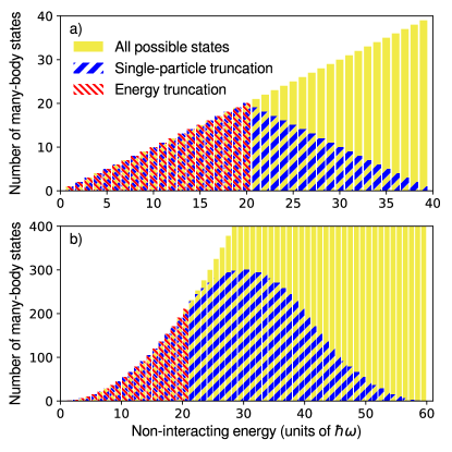
Figure 1: (Color online) Number of basis states for each value of the non-interacting energy. We consider 20 single-particle modes for $N=2$ (upper panel) and $N=3$ (lower panel). The yellow solid region is the number of states with less energy than $E=40~{}\hbar\omega$ and $E=60~{}\hbar\omega$ for two and three particles, respectively. The blue thick hatched region is the number of states that can be created with 20 single-particle states. The red thin hatched region is the number of states created with 20 single-particle states and with an energy truncation at $E=E_{\mathrm{max}}$.

III.3 Truncation of the many-body basis

As mentioned, in systems with more than two particles one first needs to truncate the many-body basis to a finite number of HO states. To do this truncation, we choose a number of modes $M$ and then simply truncate the basis up to all the states with non-interacting energy smaller or equal than $E_{\text{max}}(M)$. This energy truncation enables us to greatly reduce the size of the many-body basis while maintaining the quality of the results [30, 15].

In systems composed of bosons or distinguishable particles, as the ones considered in this work, the optimal value for this maximum energy is [30]

$$E_{\mathrm{max}}(M)/\hbar\omega=M-1+N/2\,,$$ (18)

where $N$ is the number of particles. Therefore, the basis is constructed as usual by discarding all the states with non-interacting energy larger than $E_{\mathrm{max}}$.

To illustrate the size of the truncated many-body basis, in Fig. 1 we show the number of many-body states as a function of the non-interacting energy. We compare the basis created by the energy truncation (red thin hatched region), explained before, with a standard truncation in the number of modes without the energy restriction (blue thick hatched region). With the energy restriction one considers much fewer states than with a standard truncation. However, the energy truncation provides a complete basis up to $E_{\mathrm{max}}$. In contrast, a simple truncation in the number of modes results in an inconsistent basis where some non-interacting energy states are not considered (see difference between yellow solid and blue thick hatched regions). We provide additional details in Appendix A.

Once we have created the truncated many-body basis, we numerically diagonalize the Hamiltonian for the lower part of the energy-spectrum. This diagonalization provides an approximate solution, in analogy to the truncated result for two particles [Eq. (12)]. Afterward, we correct these calculations by connecting the two-body sector of the truncated many-body results with the truncation in Sec. III.2 for two particles [Eq. (14)]. Therefore, for each obtained eigenenergy, we can correct the truncated interaction strengths $g^{\prime}$ to their physical values $g$ using Eq. (15).

We are able to perform this correction thanks to the energy truncation of the many-body basis. Indeed, because our basis includes all the center of mass and relative coordinate modes for energies up to $E_{\text{max}}$, the many-body basis contains all the modes considered in the exact two-body solution [see Sec. III.2]. In contrast, a standard truncation without the energy restriction does not fulfill this condition and thus it is not suitable for the correction procedure.

We stress that for the rest of the main text, all the results are obtained from truncations with the energy restriction (18).

III.4 A practical procedure for the correction

In practice, the algorithm to improve the results is sketched as,

1. Create the many-body basis of $N$ particles with $M$ harmonic oscillator modes and keep only the many-body states with a non-interacting energy smaller or equal than $E_{\mathrm{max}}$. This allows us to correct states with energy below $E_{\mathrm{max}}$.

2. Compute the Hamiltonan matrix for a chosen value of the interaction strength $g^{\prime}_{\alpha\beta}$.

3. Diagonalize the Hamiltonian and obtain the eigenvalues.

4. For each eigenvalue $E$, use $\nu=(E/\hbar\omega-N/2)/2$ to compute the correction $1/g_{c}$ using Eq. (15) or Eq. (17).

5. Assign the interaction strength associated to this eigenvalue $E$ using $g_{\alpha\beta}=g_{\alpha\beta}^{\prime}/(1-g_{\alpha\beta}^{\prime}/g_{c})$.

This procedure is exact for correcting the energy of two particles as we show in the following section. Interestingly, as we show in Sec. V, this method can successfully be used for more particles.

IV Results for two particles

To illustrate how the correction procedure works, we first examine its application to the two-body problem. In Fig. 2 we show the ground-state energy for two particles as a function of the interaction strength. We show results obtained with direct diagonalization, both with and without our correction scheme, and we compare them with the exact analytic results (11). We employ a small number of HO modes to better illustrate the improvement of the calculations. From now on, the values obtained with the direct diagonalization without the correction will be referred to as the truncated results and those with the correction as the corrected ones.

We find that the correction (solid line) gives perfect agreement all digits with the exact results. In particular, reproducing the Tonks limit for two particles $E_{\infty}=2\hbar\omega$ for $1/g\to 0$. In contrast, the truncated calculation (dotted line) shows a noticeable deviation from the exact solution. We have also checked that this agreement holds for the excited states. This can be expected, as the correction is exact for two particles [see Sec. III.2].

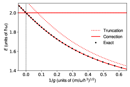
Figure 2: (Color online) Ground-state energy of the two particles system with SU(2) symmetry. The dotted line corresponds to the truncated results obtained with direct diagonalization using a basis of 20 single-particle modes, whereas the solid line corresponds to the corrected results using Eq. (17). The black circles correspond to the exact values of Eq. (11). The vertical dotted line indicates $1/g=0$. The horizontal line shows the Tonks energy for two particles.

One interesting feature of our procedure is that for a strong truncated repulsion $g^{\prime}$, the corrected physical strength $g$ becomes negative and corresponds to a strong attractive interaction. In Fig. 2, this can be appreciated when the corrected energies cross from positive to negative $g$. Indeed, when we perform a truncated diagonalization calculation for $g^{\prime}\to+\infty$, the resulting energy is greater than the Tonks solution for infinite repulsion [14]. Therefore, correcting the interaction strength, we obtain an attractive physical strength $g$ for an excited energy state in the attractive branch [20].

As a consequence, we can map all the repulsive interacting regime $g>0$ with a finite range of $g^{\prime}$. At the same time, the attractive regime $g<0$ cannot be mapped completely with a finite range of $g^{\prime}$. With this correction, we can compute the correction for the weakly-interacting regime using $g^{\prime}<0$. On the other hand, we can compute the correction for the strong attractive limit using $g^{\prime}\gg 0$

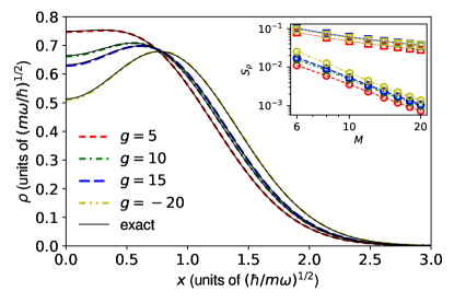
Figure 3: (Color online) Density profiles of two particles for different choices of interaction strengths $g$ (given in the labels in units of $(\omega\hbar^{3}/m)^{1/2}$). The thick lines correspond to profiles obtained with corrected direct diagonalization calculations with 20 single-particle modes, whereas the black thin lines are exact results given by Eq. (19). The inset shows a correlation parameter $S_{\rho}$ between the exact profiles (19) and the profiles obtained with the truncated diagonalizations (squares with thin lines) and the corrected ones (circles with thick lines) as a function of the number of single-particle modes $M$.

Our procedure can also be used to correct the interaction strengths associated with other properties, despite being exact only for correcting the energies of two particles. To illustrate this, in Fig. 3 we show the two-particle density profiles of the ground state for several values of $g>0$. In addition, we also depict the density profile of the first relative excitation for a large attractive interaction. We stress that the values of $g$ in the figure are those of the corrected interaction strengths. Therefore, the original truncated calculations were performed for truncated strengths $g^{\prime}$ given by Eq. (14).

We compare our results with the exact profiles obtained integrating the exact wavefunction [28]

$$\Psi(x_{1},x_{2})=Ae^{-(x_{1}^{2}+x_{2}^{2})/2}U\left(-\nu,\frac{1}{2},\frac{1}{2}(x_{1}-x_{2})^{2}\right)\,,$$ (19)

where $A$ is a normalization constant and $U(a,b,z)$ is the Tricomi function. All the parameters are in harmonic oscillator units

Our numerical calculations are in perfect agreement with the exact results, showing that our procedure also corrects the density profiles. In particular, the profile for the attractive strength $g/(\omega\hbar^{3}/m)^{1/2}=-20$ was obtained from a truncated repulsive $g^{\prime}$, showing that the previously discussed change from a repulsive to an attractive interaction is indeed correct.

To quantify the accuracy of the correction we define a correlation parameter between two density profiles as

$$S_{\rho}(\rho_{1},\rho_{2})=\frac{\int_{-\infty}^{\infty}|\rho_{1}(x)-\rho_{2}(x)|dx}{2N}\,.$$ (20)

This parameter is zero when both profiles are equal and is one when both densities do not have any common region. In the inset of Fig. 3 we show the correlation between the exact density profiles and the ones obtained from direct diagonalization as a function of the number of modes. We show the value of the parameter $S_{\rho}$ with both the original truncated calculations using $g^{\prime}=g$ (squares with thin lines) and with the corrected results (circles with thick lines). As expected, $S_{\rho}$ decreases with the number of modes for both methods, i.e. we are obtaining more precise results. In addition, not only $S_{\rho}$ has smaller values for the corrected results, it also converges to zero faster than with the truncated ones.

V Extrapolation to many particles

We now test our approach with more than two particles. We again stress that, in contrast to the two-particle case, our procedure is not exact for correcting the energy of more particles. And as we show in the following, our procedure greatly improves the truncated results.

In Fig. 4 we show the ground-state energy for $N=3$ to $N=6$ distinguishable particles with symmetric interactions $g=g_{\alpha\beta}$. We compare our results for three and four particles with exact solutions from Ref. [27]. As with the two-particle system, the original truncated calculations (thin lines) for $N=3$ and $N=4$ (left panel) show an important deviation from the exact results. In contrast, our corrected calculations (thick lines) show an almost perfect agreement with the exact solutions. We expect that this improvement holds for five and six particles (right panel).

The corrected calculations for $N\leq 5$ converge to the Tonks limit $E_{\infty}=N^{2}\hbar\omega/2$ for $1/g\sim 10^{-3}$, whereas for $N=6$ the corrected energy reaches the Tonks limit at $1/g\sim 10^{-2}$ . This larger deviation for six particles is due to the use of a small number of modes. Indeed, for $N=6$ the Tonks energy $E_{\infty}=18\hbar\omega$ is too close to the limiting energy for 20 modes. Nevertheless, this discrepancy is almost not appreciable in the figure. In contrast, the truncated calculations show a noticeable deviation, saturating to the Tonks limit at a finite interaction strength in all cases.

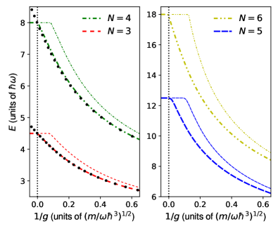
Figure 4: (Color online) Ground-state energies for $N=3$ to $N=6$ distinguishable particles computed using 20 single-particle modes. The thin lines correspond to the truncated calculations, whereas the thick lines correspond to the corrected energies obtained using Eq. (17). The black circles correspond to the exact values for $N=3$ and $N=4$ [27]. The horizontal lines correspond to states with the Tonks energy for $N$ particles.

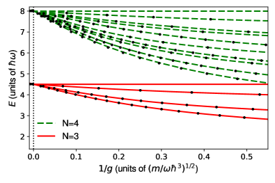
Figure 5: (Color online) Low-energy spectra for three and four particles, computed with 90 and 45 h.o. modes, respectively. The lines correspond to the corrected computations and the black circles to the exact results of Ref. [27].

In Fig. 5 we show the low-energy spectra of three and four distinguishable particles with symmetric interactions. We compare our corrected calculations (lines) with the exact solutions (circles) from Ref. [27]. We show the states that degenerate with the ground-state at the infinite interaction limit. Our correction has a great accuracy for three and four particles. The discrepancies are slightly larger for four particles. However, these discrepancies are difficult to see in the figure. We provide an additional discussion on the dependence of the energy on the number of modes in Appendix B.

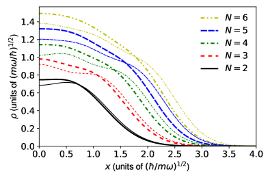
Figure 6: (Color online) Ground state density for several particles, where the thin lines are the results of the truncated results at $g^{\prime}/(\omega\hbar^{3}/m)^{1/2}=5$ and the thick lines are the corrected results at $g/(\omega\hbar^{3}/m)^{1/2}=5$.

Finally, in Fig. 6 we show the density of the ground state for several particles for a repulsive interaction strength $g/(\omega\hbar^{3}/m)^{1/2}=5$. We also show the density profiles obtained with the truncated calculation with $g^{\prime}/(\omega\hbar^{3}/m)^{1/2}=5$ in order to compare the effect of the correction. For any number of particles, the corrected density has a larger value at the center of the trap, while the tail has a smaller one. The densities corresponding to the truncated results are closer to the Tonks density profile than the corrected ones, i.e. the truncated profile has the peaks corresponding to the density profile of the infinite interacting limit whereas the corrected ones do not have it. The differences between the truncated and corrected densities increase with the number of particles. These differences can be quantified using the correlation parameter $S_{\rho}(\rho_{t},\rho_{c})$ between the truncated density $\rho_{t}$ and the corrected density $\rho_{c}$. This parameter increases (in general) as the number of particles increases, i.e. $S_{\rho}(\rho_{t},\rho_{c})=0.027$, $0.041$, $0.052$, $0.053$ and $0.050$ for two, three, four, five, and six particles, respectively.

VI Summary and conclusions

We have presented a well-defined procedure to extrapolate truncated direct diagonalization calculations for a few particles trapped in one-dimensional harmonic potentials. By employing the known two-body solution, we can correct calculations truncated to a finite number of modes $M$ to the limit of the full basis $M\to\infty$. In contrast to previous literature, [20], our method is not heuristic and does not require matching of the computed energies to the Tonks-Girardeau limit. In our case, we extrapolate the results by renormalizing the value of the interaction strength using only two-body information.

We have found that this extrapolation procedure enables us to compute the low-energy spectrum of three and four distinguishable particles with an error of less than 1% compared to exact solutions, even using a small number of single-particle modes. Furthermore, calculations for five and six particles correctly saturate to the Tonks limit. This suggests that, at least, by using the extrapolation we can provide a good qualitative description of systems with more than four particles.

The presented extrapolation is not constrained to certain particle statistics, interactions, or the number of particles. Therefore, this method can be applied to a plethora of scenarios, such as mixtures of bosonic and fermionic atoms, asymmetric interaction strengths, among others. This makes this method a good tool to study impurity physics and systems with broken SU($N$)-symmetry. In addition, the extrapolation could make accurate direct diagonalization studies with up to eight or ten particles accessible, bridging the gap between few- and many-body physics.

Appendix A Construction of the many-body basis

Particles and	Standard	Energy
modes	truncation	truncation
$N$=2, $M$=20	400	210
$N$=3, $M$=20	8 000	1 540
$N$=3, $M$=90	729 000	125 580
$N$=4, $M$=20	160 000	8 855
$N$=4, $M$=45	4 100 625	194 580
$N$=5, $M$=20	3 200 000	42 504
$N$=6, $M$=20	64 000 000	177 100

Table 1: Number of states in the many-body basis for different numbers of particles $N$ and harmonic oscillator modes $M$. We show the dimension of the Hilbert space without the energy restriction (standard truncation) and with the energy restriction (energy truncation) using $E_{\mathrm{max}}$ of Eq. (18).

To construct the many-body basis we employ single-particle states $n$ of the HO Hamiltonian. For $N$ distinguishable particles, as considered in this work, we can write one state in such basis as

$$|{\Psi}\rangle=|{n_{1},n_{2},...,n_{N}}\rangle\,,$$ (21)

where $n_{i}$ is the HO index of particle $i$.

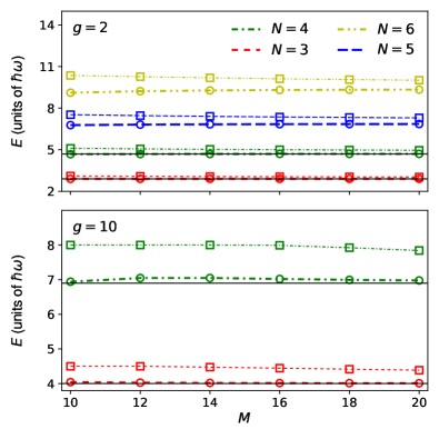
Figure 7: (Color online) Ground-state energy as a function of the number of modes $M$ for $g=2$ (upper panel) and $g=10$ (lower panel), with $g$ in units of $(\omega\hbar^{3}/m)^{1/2}$. The squares correspond to results from a truncated diagonalization, whereas the circles correspond to corrected results. The horizontal black dashed lines show the exact energies reported in Ref.[27]

In a standard truncation in the number of modes without any energy restriction, one simply considers all the states that satisfy $n_{i}\leq(M-1)\,\forall i$. This results in a Hilbert space of dimension $M^{N}$, growing extremely quickly with $M$. In contrast, within the energy truncation we consider all the states with non-interacting energy smaller or equal than $E_{\text{max}}(M)$ [Eq. (18)], that is, the states which satisfy $\sum_{i}n_{i}\leq M-1$. With this truncation scheme we can work with a much smaller dimension of the Hilbert space without affecting too much the quality of the results [30, 15]. Furthermore, and as discussed in Sec. III.3, the energy truncation allows us to correctly connect the many-body basis with the exact two-body solution.

To compare the sizes of the bases obtained with the two truncation schemes, in Table 1 we show the number of states in the many-body basis obtained with both schemes for number of particles and modes used throughout this article. We observe that, while the basis with the energy truncation grows significantly with both $N$ and $M$, it grows much slower than with the standard truncation.

Appendix B Convergence of the method

To further illustrate how the calculations depend on the number of modes $M$, in Fig. 7 we show how the ground-state energy behaves as a function of $M$ for weak and strong repulsion. We compare the results obtained from the truncated diagonalization (squares) with the ones including the correction (circles).

The corrected results depend weakly on $M$, showing that our correction produces similar results for a different number of modes, as expected. In particular, we see that for three and four particles the corrected results show only small deviations with respect to the exact solutions (black dashed lines). In contrast, the uncorrected results show important deviations from the exact and corrected results, especially for strong repulsion.

It is also worth noting that the uncorrected energies decrease with $M$ as expected from the variational principle. In contrast, the corrected energies can increase for some choices of $M$, as clearly seen with four particles in the lower panel. This means that the corrected results do not provide an upper bound for the energies. Despite this, the correction provides much more accurate results than the original truncation, making it a preferable choice in direct diagonalization calculations.

References

- Lewenstein et al. [2007] M. Lewenstein, A. Sanpera, V. Ahufinger, B. Damski, A. Sen(De), and U. Sen, Advances in Physics 56, 243 (2007).
- Bloch et al. [2008] I. Bloch, J. Dalibard, and W. Zwerger, Reviews of Modern Physics 80, 885 (2008).
- Zürn et al. [2012] G. Zürn, F. Serwane, T. Lompe, A. N. Wenz, M. G. Ries, J. E. Bohn, and S. Jochim, Phys. Rev. Lett. 108, 075303 (2012).
- Wenz et al. [2013] A. N. Wenz, G. Zürn, S. Murmann, I. Brouzos, T. Lompe, and S. Jochim, Science 342, 457 (2013).
- Zürn et al. [2013] G. Zürn, A. N. Wenz, S. Murmann, A. Bergschneider, T. Lompe, and S. Jochim, Phys. Rev. Lett. 111, 175302 (2013).
- Dalfovo et al. [1999] F. Dalfovo, S. Giorgini, L. P. Pitaevskii, and S. Stringari, Rev. Mod. Phys. 71, 463 (1999).
- Guardiola [1998] R. Guardiola, in Microscopic Quantum Many-Body Theories and Their Applications, edited by J. Navarro and A. Polls (Springer Berlin Heidelberg, Berlin, Heidelberg, 1998) pp. 269–336.
- Verstraete et al. [2008] F. Verstraete, V. Murg, and J. Cirac, Advances in Physics 57, 143 (2008).
- Grining et al. [2015a] T. Grining, M. Tomza, M. Lesiuk, M. Przybytek, M. Musiał, R. Moszynski, M. Lewenstein, and P. Massignan, Phys. Rev. A 92, 061601 (2015a).
- Deuretzbacher et al. [2007] F. Deuretzbacher, K. Bongs, K. Sengstock, and D. Pfannkuche, Phys. Rev. A 75, 013614 (2007).
- Raventós et al. [2017] D. Raventós, T. Graß, M. Lewenstein, and B. Juliá-Díaz, Journal of Physics B: Atomic, Molecular and Optical Physics 50, 113001 (2017).
- Carleo and Troyer [2017] G. Carleo and M. Troyer, Science 355, 602 (2017).
- Sowiński et al. [2013] T. Sowiński, T. Grass, O. Dutta, and M. Lewenstein, Phys. Rev. A 88, 033607 (2013).
- Rojo-Francàs et al. [2020] A. Rojo-Francàs, A. Polls, and B. Juliá-Díaz, Mathematics 8, 1196 (2020).
- Chrostowski and Sowiński [2019] A. Chrostowski and T. Sowiński, Acta Physica Polonica A 136, 566 (2019), arXiv:1908.02084 [physics.comp-ph] .
- García-March et al. [2014] M. A. García-March, B. Juliá-Díaz, G. E. Astrakharchik, T. Busch, J. Boronat, and A. Polls, New Journal of Physics 16, 103004 (2014).
- Sowiński and García-March [2019] T. Sowiński and M. Á. García-March, Reports on Progress in Physics 82, 104401 (2019).
- Mujal et al. [2017] P. Mujal, E. Sarlé, A. Polls, and B. Juliá-Díaz, Phys. Rev. A 96, 043614 (2017).
- Mujal et al. [2020] P. Mujal, A. Polls, and B. Juliá-Díaz, Phys. Rev. A 101, 043619 (2020).
- Ernst et al. [2011] T. Ernst, D. W. Hallwood, J. Gulliksen, H.-D. Meyer, and J. Brand, Phys. Rev. A 84, 023623 (2011).
- Jeszenszki et al. [2018] P. Jeszenszki, H. Luo, A. Alavi, and J. Brand, Phys. Rev. A 98, 053627 (2018).
- Lindgren et al. [2014] E. J. Lindgren, J. Rotureau, C. Forssén, A. G. Volosniev, and N. T. Zinner, New Journal of Physics 16, 063003 (2014).
- Dehkharghani et al. [2015] A. Dehkharghani, A. Volosniev, J. Lindgren, J. Rotureau, C. Forssén, D. Fedorov, A. Jensen, and N. Zinner, Scientific Reports 5, 10675 (2015).
- Grining et al. [2015b] T. Grining, M. Tomza, M. Lesiuk, M. Przybytek, M. Musiał, P. Massignan, M. Lewenstein, and R. Moszynski, New Journal of Physics 17, 115001 (2015b).
- Rotureau [2013] J. Rotureau, Eur. Phys. J. D 67, 153 (2013).
- Rammelmüller et al. [2022] L. Rammelmüller, D. Huber, and A. G. Volosniev, (2022), arXiv:2202.04603 [cond-mat.quant-gas] .
- Laird et al. [2017] E. K. Laird, Z.-Y. Shi, M. M. Parish, and J. Levinsen, Phys. Rev. A 96, 032701 (2017).
- Busch et al. [1998] T. Busch, B.-G. Englert, K. Rzażewski, and M. Wilkens, Foundations of Physics 28, 549 (1998).
- Stoof et al. [2009] H. T. C. Stoof, K. B. Gubbels, and D. Dickerscheid, Ultracold Quantum Fields (Springer, Dordrecht, 2009).
- Płodzień et al. [2018] M. Płodzień, D. Wiater, A. Chrostowski, and T. Sowiński, (2018), arXiv:1803.08387 [cond-mat.quant-gas] .