Revisiting WASP-47 with ESPRESSO and TESS

Abstract

WASP-47 hosts a remarkable planetary system containing a hot Jupiter (WASP-47 b; P = $4.159$ days) with an inner super-Earth (WASP-47 e; P = $0.7896$ days), a close-orbiting outer Neptune (WASP-47 d; P = $9.031$ days), and a long period giant planet (WASP-47 c; P = $588.4$ days). We use the new TESS photometry to refine the orbital ephemerides of the transiting planets in the system, particularly the hot Jupiter WASP-47 b, for which we find an update equating to a 17.4 min shift in the transit time. We report new radial velocity measurements from the ESPRESSO spectrograph for WASP-47, which we use to refine the masses of WASP-47 d and WASP-47 e, with a high cadence observing strategy aimed to focus on the super-Earth WASP-47 e. We detect a periodic modulation in the K2 photometry that corresponds to a 32.5$\pm$3.9 day stellar rotation, and find further stellar activity signals in our ESPRESSO data consistent with this rotation period. For WASP-47 e we measure a mass of $6.77\pm 0.57$ M_⊕ and a bulk density of $6.29\pm 0.60$ g cm^-3, giving WASP-47 e the second most precisely measured density to date of any super-Earth. The mass and radius of WASP-47 e, combined with the exotic configuration of the planetary system, suggest the WASP-47 system formed through a mechanism different to systems with multiple small planets or more typical isolated hot Jupiters.

1 Introduction

The formation mechanisms for hot Jupiter planets ($\mbox{R${}_{P}$}>0.6\,\mbox{R${}_{J}$}$; $P<10$ days) remain uncertain, although viable formation pathways have been proposed (Dawson & Johnson, 2018). One possible scenario is that hot Jupiters begin their formation at large orbital distances and then migrate towards the star during formation (eg. Lin et al., 1996; Nelson et al., 2000). This planetary migration could arise from multiple causes, such as interactions between the protoplanet and the circumstellar disk (Papaloizou & Larwood, 2000) or through some form of high eccentricity migration, which can be triggered by planet-planet scattering (Chatterjee et al., 2008) or secular interactions between multiple bodies, including Kozai-Lidov cycles (Kozai, 1962; Lidov, 1962). This high eccentricity migration removes inner planets from the system (Mustill et al., 2015), leaving most hot Jupiter planets isolated and without other planetary companions in close orbits (eg. Steffen et al., 2012). The observational evidence seems to support this model. The vast majority of hot Jupiters do not have close orbiting companions, although many have long-period massive outer companions (eg. Knutson et al., 2014). For the longer period warm Jupiters the situation is different, and warm Jupiter planets are significantly more likely to be accompanied by closely orbiting small planetary companions (Huang et al., 2016). A possible explanation for this is that these warm Jupiters are forming in-situ, as opposed to migrating from outer regions.

Out of the hundreds of hot Jupiters discovered to date, only three have been found to also host small, inner planets: Kepler-730c (Cañas et al., 2019), TOI-1130c (Huang et al., 2020), and WASP-47 b (Hellier et al., 2012). The 55-Cancri system (Bourrier et al., 2018) is also similar to the WASP-47 system in that it contains a super-Earth with an orbital period shorter than one day (55-Cancri e), and close–in giant planet (55-Cancri b; 14.6 days). As a result of the brightness of the host star (V = 5.95 mag), the 55-Cancri system, and particularly 55-Cancri e, have been very well studied (eg. Demory et al., 2012; Tsiaras et al., 2016; Angelo & Hu, 2017).

Since the configurations of these three systems bears more resemblance to the population of warm Jupiters than to the hot Jupiters  it has been speculated that perhaps these systems also formed through an in-situ pathway (Huang et al., 2020). It is therefore imperative to study these three systems in detail to determine if there is any other evidence that they formed from a different pathway to the majority of hot Jupiter systems. In order to do this, we require precise knowledge of the planetary system parameters, especially the planetary masses, densities, and orbital periods.

WASP-47 has been extensively studied since its discovery in 2012. Initially, WASP-47 was shown to to host a $4.159$ day period transiting hot-Jupiter WASP-47 b (Hellier et al., 2012). Later, an extensive spectroscopic monitoring campaign revealed the presence of the $588.4$ day giant planet WASP-47 c (Neveu-VanMalle et al., 2016). It is not currently known whether or not WASP-47 c transits the star, although Vanderburg et al. (2017) derived a 10% probability that it does transit. This estimate is greater than the geometric probability ($\approx$ 0.6%) and arises from additional dynamical constraints placed by the stability of the inner WASP-47 system on the inclination of WASP-47 c. Most surprisingly, two additional small planets were discovered through photometric monitoring (Becker et al., 2015) with the Kepler space telescope during the K2 mission (Howell et al., 2014). WASP-47 d is a Neptune-mass planet exterior to the hot Jupiter, while WASP-47 e is a super-Earth interior to the hot Jupiter. The orbital configuration of the inner regions of this remarkable planetary system are shown in Figure 1.

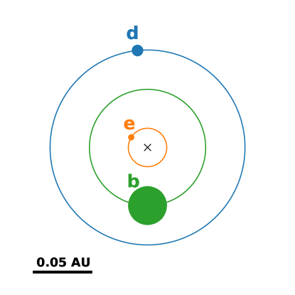
Figure 1: Orbital configuration of the inner three planets in the WASP-47 system. The three lines show the orbits of the planets: WASP-47 b (green), WASP-47 d (blue), WASP-47 e (orange). The position of the WASP-47 star is depicted by the black cross. The filled circles give the positions of the planets at T = 2549449.35 BJD, which is the time of the first transit of WASP-47 b observed by TESS, assuming observer viewing from bottom of plot and orbits in the anti-clockwise direction. The relative sizes of the filled circles are proportional to the the relative radii of the planets.

Table 1: Key Stellar Properties for WASP-47

Property	Value	Source
TIC	102264230	TICv8
RA (deg)	$331.20309414396$	Gaia EDR3
Dec (deg)	$-12.01907283535$	Gaia EDR3
$\mu_{\rm RA}$ (mas)	$15.074\pm 0.020$	Gaia EDR3
$\mu_{\rm Dec}$ (mas)	$-41.467\pm 0.020$	Gaia EDR3
Parallax (mas)	$3.7010\pm 0.0201$	Gaia EDR3
V (mag)	$11.936\pm 0.046$	TICv8
B (mag)	$12.736\pm 0.024$	TICv8
TESS (mag)	$11.29\pm 0.0061$	TICv8
Gaia G (mag)	$11.7817\pm 0.0028$	Gaia EDR3
Gaia bp (mag)	$12.1716\pm 0.0029$	Gaia EDR3
Gaia rp (mag)	$11.2294\pm 0.0038$	Gaia EDR3
J (mag)	$10.613\pm 0.022$	2MASS
H (mag)	$10.310\pm 0.022$	2MASS
K (mag)	$10.192\pm 0.026$	2MASS
M∗ (M⊙)	1.040 $\pm$ 0.031	V2017
R∗ (R⊙)	1.137 $\pm$ 0.013	V2017
$\rho_{*}$ (g cm-3)	0.998 $\pm$ 0.014	Section 3.1
$T_{\rm eff}$ (K)	5552 $\pm$ 75	V2017
[Fe/H]	0.38 $\pm$ 0.05	V2017
$\log g$(cgs)	$4.3437\pm 0.0063$	V2017
TICv8 - Stassun et al. (2019)
Gaia EDR3 - Gaia Collaboration et al. (2021)
2MASS - Skrutskie et al. (2006)
V2017 - Vanderburg et al. (2017)

Further to these discovery papers, there have been many independent efforts to measure the masses of the planets in the WASP-47 system. Multiple radial velocity monitoring campaigns using the PFS (Dai et al., 2015), HIRES (Sinukoff et al., 2017), and HARPS-N (Vanderburg et al., 2017) spectrographs have been carried out. Dynamical analyses have also been performed to determine the masses of the planets (eg. Almenara et al., 2016; Weiss et al., 2017). These different studies reached slightly differing conclusions about the mass, and therefore the composition, of WASP-47 e.

In addition to the consequences for planetary formation, WASP-47 e represents one of the best cases to study the composition of a super-Earth like planet, thanks to the wealth of data available on the system. Therefore, we seek to shed yet more light on this system.

In this work we use the next generation of high precision spectrographs, ESPRESSO, in order to obtain the most precise and accurate measurements of the planet masses and densities, particularly focusing on the super-Earth WASP-47 e.

2 Observations

2.1 ESPRESSO

ESPRESSO (Echelle SPectrograph for Rocky Exoplanets and Stable Spectroscopic Observations; Pepe et al., 2020) is a new high-resolution, visible spectrograph operating at the VLT at ESO’s Paranal Observatory in Chile. ESPRESSO can be fed from any of the 8.2 m Unit Telescopes and can also be fed simultaneously by all four. The three main exoplanet science objectives of ESPRESSO are to find new Earth-mass planets orbiting in the habitable zone of Sun-like stars, characterize the atmospheres of exoplanets, and precisely determine the masses of low-mass transiting exoplanets. ESPRESSO has already been used to confirm TESS discoveries, including LP 714-47 b (TOI-442 b; Dreizler et al., 2020), TOI-130 b (Sozzetti et al., 2021), and the planets in the TOI-178 system (Leleu et al., 2021). ESPRESSO radial velocity measurements have also been used to improve upon the precision of the masses of LHS-1140 b and c (Lillo-Box et al., 2020).

ESPRESSO operates in the wavelength range 380–788 nm, and is designed to achieve radial velocity precision of 10 cm s^-1 for bright stars (V ¡ 8 mag) in order to be capable of detecting Earth-mass planets around solar type stars. This unprecedented radial velocity precision is achieved both by building on and improving the technologies used in the HARPS spectrograph for stability and calibration accuracy but also through the increased light-collecting capacity of the VLT UTs compared to the ESO 3.6 m.

WASP-47 was observed by ESPRESSO between the dates of 2019 6 August and 30 September (Run ID: 0103.C-0422; PI Bayliss), using an exposure time of 1250 seconds and with an airmass limit of z ¡ 1.5 for each observation. We reduced all the spectra using the ESPRESSO reduction pipeline (version 2.2.1) through the ESOReflex workflow environment (Freudling et al., 2013). The signal-to-noise achieved from our observations ranged from 40-60 at $\lambda$ = 550 nm. The radial velocity CCFs were computed using a G9 mask, and the pipeline automatically extracts diagnostic information on the CCFs, including the FWHM of the CCF. In total, WASP-47 was observed 25 times by ESPRESSO. Two of these observations show anomalous CCF profiles likely caused by cloud coverage and/or moon contamination, and are not used in the analysis. An additional four observations were identified as having been taken during a transit of WASP-47 b. We also remove these from our analysis so that the Rossiter-McLaughlin signal of WASP-47 b (Sanchis-Ojeda et al., 2015) does not affect our radial velocity model and analysis. This left us with 19 radial velocity measurements from ESPRESSO for our analysis. We run spectral analysis on our co-added ESPRESSO spectra using the ESPRESSO-DAS pipeline. The values we derive for effective temperature and metallicity are consistent with those derived by Vanderburg et al. (2017).

In addition to the ESPRESSO data, we utilize a number of archival radial velocity measurements of WASP-47, which were obtained using the HARPS-N (69 data points with mean a precision of 3.2 ms^-1; Vanderburg et al., 2017), HIRES (43 data points with mean a precision of 2.0 ms^-1; Sinukoff et al., 2017), PFS (26 data points with mean a precision of 3.2 ms^-1; Dai et al., 2015), and CORALIE (52 data points with mean a precision of 12.5 ms^-1; Neveu-VanMalle et al., 2016) spectrographs. We did not perform any additional reduction of these data sets.

2.2 K2

As we discuss in Section 3, a degree of variability in the radial velocity data indicates relatively strong stellar activity on WASP-47. In order to help understand and account for this activity, we turned to the high precision time series photometry for WASP-47 from the Kepler space telescope (Borucki et al., 2010).

WASP-47 was observed by the Kepler space telescope during Campaign 03 of the K2 mission (Howell et al., 2014). WASP-47 was observed continuously for 67 days between the dates of 2014 November 17 and 2015 January 23. WASP-47 was observed in the short cadence mode, and a short cadence light curve was extracted by Becker et al. (2015) using the method of Vanderburg et al. (2015). We accessed this light curve for the transit analysis performed in this work.

2.3 TESS

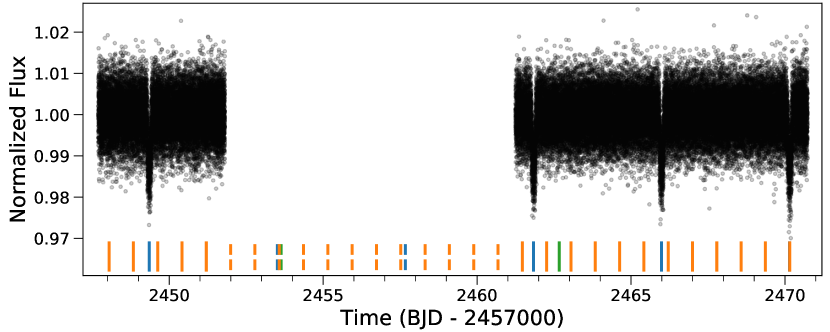
Figure 2: TESS 20 s PDCSAP_FLUX photometry for WASP-47. The colored bars at the bottom show the positions of the transits of WASP-47 b (blue), WASP-47 d (green), and WASP-47 e (orange), with the dashed bars showing the positions of transits which fall in the large data gap caused by Earth and Moon crossing events.

WASP-47 was observed by the TESS mission (Ricker et al., 2014) during Sector 42 between the dates of 2021 August 21 and September 15. WASP-47 fell on camera 1 CCD 4. We utilized the 20 second cadence light curve produced by the SPOC pipeline (Jenkins et al., 2016), which we downloaded from MAST. We use the PDCSAP_FLUX time series in this work, which has had instrumental and blending effects corrected in the light curve (Jenkins et al., 2016).

During both orbits of Sector 42, the Earth crossed the field of view of camera 1, with the Moon also crossing the field of during the first orbit. Due to the significant increases in scattered light in the background during these events, the PDCSAP_FLUX time series spans only 4.11 days in the first orbit and 9.48 days in the second, giving a total of around half the nominal 27 day coverage for a given sector. The TESS light curve is shown in Figure 2.

3 Analysis

3.1 Transit Analysis

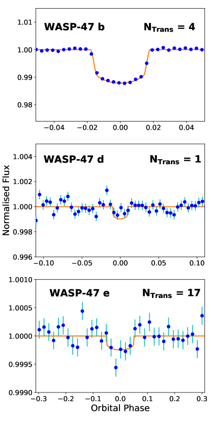
Figure 3: Phase-folded TESS photometry of WASP-47 zoomed around the transit events for Top: WASP-47 b Middle: WASP-47 d and Bottom: WASP-47 e. For all panels the photometry (blue circles) has had the transit models from the other two planets subtracted and is binned in phase on a time scale of 20 minutes for WASP-47 b and WASP-47 e and 60 minutes for WASP-47 d. The orange lines show the best fit transit models from the modelling in Section 3.1.

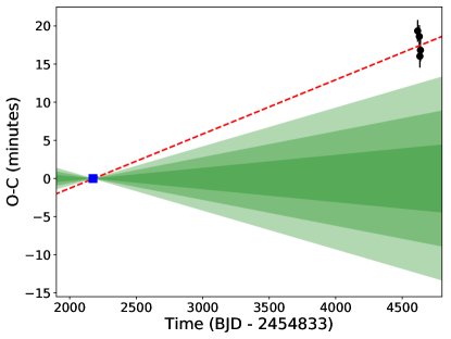
Figure 4: Measured transit times for WASP-47 b transit events in the TESS data (black circles) compared with the literature ephemeris (blue square and green shaded regions) from Becker et al. (2015). The uncertainties on the TESS transit times have had an additional 1 minute added in quadrature to account for the TTVs of WASP-47 b. The shaded green regions give the 1, 2, and 3 $\sigma$ uncertainties of the predicted ephemeris from Becker et al. (2015). The red dashed line represents the updated ephemeris determined in this work.

We analysed the TESS data in order to refine the planetary parameters of the WASP-47 planets. It is not known if WASP-47 c transits the host star (Neveu-VanMalle et al., 2016). However based on the best ephemeris for WASP-47 c  it is not expected to transit during the TESS monitoring; the next conjunction of WASP-47 c is predicted to occur just under 60 days after the end of the TESS observations. We searched the light curve evidence of of any previously unknown transiting planets. We mask out the transits of WASP-47 b, d, and e, and search for additional transit signals using BLS (Kovács et al., 2002) but we do not find any evidence for a previously unknown transiting planet. Therefore, we consider just WASP-47 b, d, and e in this analysis.

We model the transit light curves of the three planets using batman (Kreidberg, 2015) with the following free parameters: the times of transit center, $T_{C}$, the orbital periods of the planets, $P$, the planet-to-star radius ratios, $R_{P}/R_{*}$, the orbital inclinations, $i$, and the stellar density, $\rho_{*}$, from which we can compute the scaled semi-major axes, $a/R_{*}$. For $T_{C}$ and $P$ we use wide uniform priors centred on the values derived by Becker et al. (2015). For $R_{P}/R_{*}$ and $i$ we use uniform priors between 0 and 1 and between 0^∘ and 90^∘ respectively. For $\rho_{*}$ we use another wide uniform prior between 0.9 and 1.1, based on the prior knowledge of the stellar parameters from Vanderburg et al. (2017). We use a quadratic limb-darkening law with two independent sets of coefficients for the K2 and TESS data. We sampled for these coefficients using the parameterization of Kipping (2013). For the analysis of WASP-47 b and WASP-47 e we adopted circular orbits based on the findings of Vanderburg et al. (2017) that the tidal circularization timescales for these two planets are significantly shorter than the age of the system. We allow for a non-circular orbit for WASP-47 d and impose a half-Gaussian prior with a width of 0.014 and centered on 0 for $e_{d}$. This constraint on the eccentricity of WASP-47 d comes from the dynamical analyses performed independently by Becker et al. (2015) and Weiss et al. (2017). This eccentricity is taken into account when calculating the value of $a/R_{*}$ from $\rho_{*}$ for the orbit of WASP-47 d. We explore the parameters using a Monte Carlo Markov Chain (MCMC) analysis using the emcee Ensemble Sampler (Foreman-Mackey et al., 2013). A total of 48 walkers were run for a burn in of 3000 steps followed by a further 10000 steps per chain to sample the posterior distribution. We calculated the autocorrelation lengths, $\tau$, for each parameter and find $\tau\ll N/100$, where $N$ is the chain length, indicating good convergence for all parameters except $\omega_{d}$ which has $\tau=N/26.5$. This is unsurprising, as due to the eccentricity of WASP-47 d being low and consistent with 0 at 2$\sigma$, from the transit light curves alone we cannot place strong constraints on $\omega_{d}$ and so do not expect excellent convergence. The transit models recovered from this analysis are plotted in Figure 3. The planetary radii we derive are reported in Table 3. From this analysis, we obtain a stellar density of $\rho_{*}=0.998\pm 0.014$ g cm^-3, which we note is consistent with the current best estimates for the stellar mass and radius (Vanderburg et al., 2017).

Compared to the parameters from just the K2 photometry alone, the inclusion of the TESS photometry into the analysis does not provide additional information on the radii of the planets. This is a result of both the reduced time coverage of the TESS photometry compared to the K2 (13.59 days vs 67 days) and the significantly reduced photometric precision (3040 ppm-per-minute vs 350 ppm-per-minute). In particular, WASP-47 d transited just once during the available TESS photometry (see Figure 2), and so the recovery of the transit in the TESS data is marginal.

TESS data have provided a useful method for refining the ephemerides for known transiting hot Jupiters by increasing the baseline of transit observations (Shan et al., 2021). We are able to take advantage of this method by increasing the baseline of observations to refine the orbital periods of the WASP-47 planets. For the hot Jupiter WASP-47 b our results yield an orbital period of 4.1591492$\pm$0.0000006 days, which is significantly (4.15 $\sigma$) longer than the current literature value (Becker et al., 2015) (see Figure 4). We also reduce the uncertainty on this period by a factor of seven. WASP-47 b displays transit timing variations with an amplitude on the order of 1 minute (Becker et al., 2015) however these cannot account for the offset in transit times observed, which has a magnitude of 17.4 minutes. For WASP-47 d we find an orbital period of 9.03055$\pm$0.00008 days, which is slightly shorter than the Becker et al. (2015) period, but only differs by just over 1$\sigma$. We have reduced the uncertainty on this period by a factor of 2.4. For the super Earth WASP-47 e our measured orbital period of 0.789595$\pm$0.000005 days agrees with the Becker et al. (2015) results, but again we significantly improve the precision on this measurement by a factor of 3.6.

3.2 Radial Velocity Analysis

We modelled our ESPRESSO radial velocity data along with the archival data from HARPS-N, HIRES, and CORALIE using the exoplanet Python package (Foreman-Mackey et al., 2020). The exoplanet package allows for robust probabilistic modelling of astronomical time series data using PyMC3. We used exoplanet to model the multiple radial velocity data sets using the No U-Turns Sampler Hamiltonian Monte Carlo method.

The free system parameters included in the analysis were the orbital periods of the planets, $P_{i}$, the times of conjunction, $T_{C,i}$, and the radial velocity semi-amplitudes, $K_{i}$, where $i$ represents the planets $b,c,d,\&\,e$. For $P_{i}$ and $T_{C,i}$ we used Gaussian priors taken from the posteriors of the transit analysis. We also fitted for the eccentricities and arguments of periastron of planets c and d, $e_{c},e_{d},\omega_{c},\omega_{d}$. As with the transit analysis, we fix $e_{b}=e_{e}=0$, and for $e_{d}$ we imposed a half-Gaussian prior with a width of 0.014 and centered on 0. For $e_{c}$ we use a uniform prior constraining the eccentricity to be between 0 and 1. For $\omega_{c}$ and $\omega_{d}$ we used uniform priors between -180^∘ and +180^∘. We also include a white noise jitter term, $\sigma$, and a systemic radial velocity, $\gamma$, for each instrument. For CORALIE, we use independent jitter and systemic velocity terms for the data taken before and after the upgrade in November 2014.

The archival PFS data (Dai et al., 2015) has been excluded from prior analyses on WASP-47 due to the presence of large scatter in the radial velocities and the high risk of contamination from systematic errors (Vanderburg et al., 2017). From our initial modelling, we also find a large jitter term is required for the PFS data. Motivated by this, we investigated the effect had by excluding the PFS data from our analysis. We find that the derived parameter values, specifically $K_{i}$, are unaffected by including the PFS data, and that the maximum log-likelihood value obtained during the sampling increases when the PFS data are not included in the analysis. Therefore, we also exclude the PFS data from our analysis.

From this initial modelling, we found a significant jitter term was required for our ESPRESSO data. The value required was $\sigma_{\rm ESP}=3.25$ ms^-1, compared to the median photon-limited uncertainty of 0.55 ms^-1 for the ESPRESSO radial-velocities. Motivated by this we searched for evidence of periodicity in the residuals to the initial model. This excess scatter in the ESPRESSO radial-velocities suggests the presence of additional noise that we have not accounted for in our model. This additional noise is likely to arise from the stellar activity of WASP-47. We studied the available data for WASP-47 to investigate any evidence for stellar variability.

3.3 Stellar Rotation Analysis

Vanderburg et al. (2017) used the HARPS-N spectra to derive a maximum stellar rotational velocity of 2 kms^-1 based on the line broadening of the stellar absorption lines. This implies a minimum rotation period of $P_{\rm Rot;\ min}$ = $28.762$ days. Independently, Sanchis-Ojeda et al. (2015) derived a value of $v\sin i=1.8^{+0.24}_{-0.16}$ km s^-1 from their Rossiter-McLaughlin analysis of WASP-47 b. From this measurement we estimate a rotation period of WASP-47 of $P_{\rm Rot}$ = 31.96$\pm$4.36 days. These $P_{\rm Rot}$ estimates are assuming WASP-47 is aligned along our line–of–sight. This is a reasonable assumption given the Rossiter-McLaughlin measurement of a spin aligned orbit for WASP-47 b (Sanchis-Ojeda et al., 2015). These $P_{\rm Rot}$ limits and estimates will be important for properly interpreting our rotation analyses.

3.3.1 Photometric Rotation Analysis

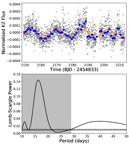
Figure 5: Top: K2 photometry from campaign 3 for WASP-47 used for the rotation analysis in this work. The grey points show the detrended data (see Section 3.3.1) and the blue points give the data binned to a timescale of 1 day. The orange line shows the most significant Lomb-Scargle period of 16.26 days with an amplitude of 0.1 mmag. Bottom: Lomb-Scargle periodogram for the K2 photometry. As with Fig. 6 the shaded area highlights the rotation periods excluded by the minimum $P_{\rm Rot}$ =$P_{\rm Rot;\ min}$. The significant peak at 16.26  days likely corresponds to half the true rotation period. The horizontal lines give the 0.1% (solid) and 0.01% (dashed) false alaram probabilities respectively.

We used the K2 data of WASP-47 to search for photometric signs of stellar activity. Stellar spots are cooler and less bright than the majority of the stellar surface. As the star rotates, these spots rotate into and out of view of the telescope, resulting in a sinusoidal-like variation in the photometric data at the rotation period of the star, or some harmonic of this period. During the production of the K2 short cadence light curve, long term photometric variations were fitted and removed using a spline (Becker et al., 2015). It is these exact variations that we want to study here. Therefore, we use a different long cadence K2 light curve that had been reduced using the ”self-flat-fielding” method (Vanderburg & Johnson, 2014). This reduction technique significantly improves upon the precision of the raw K2 photometry and in most cases gets to a precision within a factor of two of the photometry delivered by Kepler during the nominal mission (Vanderburg & Johnson, 2014). More importantly, this method preserves long term astrophysical variations in the photometry.

We used the orbital parameters from Becker et al. (2015) to remove any data points taken during a transit of any of the three WASP-47 transiting planets. We also excluded the data points during two sharp ramps. These two ramps are related to the settling of the roll of the spacecraft at the start of the campaign and after the change in the roll direction around 50 days into the campaign. We fit quadratic polynomials to the two remaining continuous data chunks in order to remove long-term systematic trends in the data believed to be spacecraft systematics rather than astrophysical in nature. The detrended K2 photometry is shown in Figure 5.

We ran a Lomb-Scargle analysis on the remaining out-of-transit photometry. The resultant periodogram is shown in the bottom panel of Figure 5. The K2 photometry displays some sign of periodicity on periods which are similar to those present in the ESPRESSO data. However due to the 67 day length of the K2 photometry and the detrending methods applied, this period search becomes less sensitive for longer period signals, especially for signals around half the monitoring length and longer. The significant peak in the K2 periodogram is at a period of 16.26$\pm$1.94 days. This period is shorter than the $P_{\rm Rot;\ min}$ limit set by Vanderburg et al. (2017). Periodic signals are expected in photometric time series at the second harmonic of the rotation period (Clarke, 2003). Particularly in cases where there are multiple active regions of the surface of the star where the largest peak in the periodogram can be at half the true rotation period (eg. McQuillan et al., 2013). Therefore, this 16.26$\pm$1.94  day signal likely corresponds to half the true rotation period of WASP-47, giving a rotation period of $P_{\rm Rot}$ = 32.5$\pm$3.9 days, which is consistent with the prediction from the Sanchis-Ojeda et al. (2015) $v\sin i$ measurement.

We also turn to theoretical predictions for stellar rotation periods to confirm that this value is a physically reasonable rotation period for WASP-47. We use the model from Barnes (2007) which estimates $P_{\rm Rot}$ given the stellar magnitudes in the $B$ and $V$ pass-bands and the age of the star. For WASP-47, we have magnitudes of $V=$ 11.936 mag and $B=$ 12.736 mag, and by assuming a solar age of 4.5 Gyr we find a predicted rotation period of $P_{\rm Rot}$${}_{\rm;\ pred}\,=\,34.96$ days.

We note that Hellier et al. (2012) searched the WASP photometry of WASP-47 for signs of stellar rotation and did not find any significant rotational modulation, placing an upper limit of 0.7 mmag for the amplitude of any such modulation. From the K2 photometry in Figure 5, the peak-to-peak amplitude of the modulation is approximately 0.1 mmag, therefore the non-detection of rotational modulation in the WASP photometry is not inconsistent with the K2 detection. Similarly, due to the short time coverage and low precision, the TESS data, is unable to help constrain the stellar rotation.

3.3.2 Spectroscopic Rotation Analysis

Figure 6: Generalized Lomb-Scargle periodograms for: Top: ESPRESSO radial velocity residuals to the initial model from Section 3.2; Middle: the ESPRESSO CCF FWHM measurements; Bottom: measurements of $\log R^{\prime}_{\rm HK}$ from the ESPRESSO spectra. The solid vertical blue line denotes the rotation period of $P_{\rm Rot}$ = 32.5 days derived from the K2 photometry, with the vertical dashed blue lines marking $P_{\rm Rot}$/2 and $P_{\rm Rot}$/3 harmonics. The shaded area highlights stellar rotation periods that are excluded by the calculated minimum rotation period of $28.762$ days. The horizontal lines indicate the 1% (dashed) and 10% (solid) false alarm probabilities.

We search for periodic signals in our spectroscopic ESPRESSO data that might provide evidence that the excess scatter seen in the ESPRESSO radial velocities arises as a result of stellar activity. We ran a generalized Lomb-Scargle analysis on the residuals to the model from the fitting in Section 3.2, which revealed periodicities at periods of roughly 35 and 18 days, as shown in Figure 6. We also searched for periodic signals in the ESPRESSO CCF FWHM measurements, as the FWHM of the CCF has been shown to act as a stellar activity indicator (Boisse et al., 2011; Oshagh et al., 2017). Stellar spots suppress the flux contributions from different sections of the stellar surface to the stellar lines and thus and modify the CCF profile. Spots on the limb of the star suppress the wings of the line, resulting in the CCF profile showing a smaller FWHM. Conversely, spots on the center of the stellar disc affect the center of the stellar lines, resulting in a wider CCF FWHM (Boisse et al., 2011). Periodic signals with the same periods as those found in the RV residuals were found in the CCF FWHM measurements (see Figure 6). Boisse et al. (2011) also find that the stellar activity causes the CCF contrast, the fractional height of the CCF peak, to anti-correlate with the FWHM. We compare the contrast and FWHM for the ESPRESSO CCFs and find a strong anti-correlation (see Figure 7). This anti-correlation is in line with the predictions and strengthens the confidence that the variations in the CCF FWHM, and by extension the ESPRESSO radial velocity residuals, are a result of stellar activity.

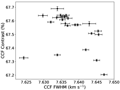
Figure 7: The contrast and FWHM values for the ESPRESSO cross-corelation functions for our observations of WASP-47. We see a strong anti-correlation, indicative of spot-induced stellar activity (Boisse et al., 2011).

We also used the Ca-II H and K lines in the ESPRESSO spectra to determine values of the activity index $\log R^{\prime}_{\rm HK}$. Running a further Lomb-Scargle analysis on this activity indicator reveals a periodic signal in the range 30-40 days with a peak around 33 days (Figure 6).

3.4 Stellar Activity Analysis

We expect the spectroscopic signals from stellar activity to manifest at periods equal to $P_{\rm Rot}$ and at the $P_{\rm Rot}$/2 and $P_{\rm Rot}$/3 harmonics (Boisse et al., 2011). From the ESPRESSO radial velocity periodogram (top panel of Figure 6), we see a signal close to P=35 days, with harmonics close to P/2 and P/3. These peaks are also seen in the CCF FWHM periodogram, although an extra peak is seen close to 27 days that is likely due to the moon. The $\log R^{\prime}_{\rm HK}$ activity index from the ESPRESSO spectra has a peak in the periodogram at approximately 33 days.

The periodicities detected in the ESPRESSO RV residuals and activity indicators are consistent with the 32.5$\pm$3.9 day rotation period derived from the K2 photometry for WASP-47. Based on the continuous coverage and very high precision of the K2 data, we take the K2 $P_{\rm Rot}$ value as the most probable rotation period.

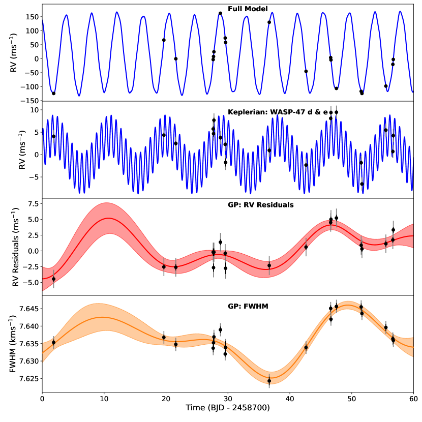
Figure 8: ESPRESSO time series data for WASP-47. Top: ESPRESSO radial velocity measurements with the systemic velocity $\gamma_{\rm ESP}$ subtracted. The blue line gives the full Keplerian model for all four planets and the GP. Second: ESPRESSO radial velocity measurements with $\gamma_{\rm ESP}$, the Keplerian models for WASP-47 b and c, and the GP model subtracted. The blue line gives the two-planet Keplerian model for WASP-47 d and e. Third: ESPRESSO radial velocity residuals to the four-planet Keplerian model. The red line gives the GP model and the shaded area provides the 1$\sigma$ confidence interval of the GP. Bottom: FWHM measurements of the ESPRESSO CCFs. The orange line gives the GP model and the shaded area provides the 1$\sigma$ confidence interval of the GP.

3.5 Gaussian Process Analysis

We utilize a Gaussian Process (GP) kernel with a periodicity close to $P_{\rm Rot}$ = 32.5 days in order to accurately model the radial velocity variability due to spot rotation. We use the celerite2 rotation term kernel constructed from two Simple Harmonic Oscillator (SHO) terms at $P_{\rm Rot}$ and $P_{\rm Rot}$/2, implemented using the exoplanet (Foreman-Mackey et al., 2020) and celerite2 (Foreman-Mackey et al., 2017a; Foreman-Mackey, 2018a) Python packages. A single SHO term is given by

$$\small\kappa(\tau)=\sigma_{GP}^{2}\exp\left(-\frac{\pi\tau}{QP_{\rm Rot}}\right)\left[\cos\left(2\pi\eta\frac{\tau}{P_{\rm Rot}}\right)+\frac{1}{2\eta\,Q}\sin\left(2\pi\eta\frac{\tau}{P_{\rm Rot}}\right)\right]$$ (1)

where $\eta=|1-(4Q^{2})^{-1}|^{1/2}$. The rotation term kernel takes as its hyperparameters: the standard deviation of the process, $\sigma_{GP}$, which is related to the amplitude of the variability signal, the stellar rotation period, $P_{\rm Rot}$, the signal quality, $Q$, the difference in signal quality between the $P_{\rm Rot}$ and $P_{\rm Rot}$/2 modes, $\Delta Q$, such that $Q_{P_{\rm Rot}}=Q_{P_{\rm Rot}/2}+\Delta Q$, and the mix factor between the two modes, $f$, such that $\sigma_{P_{\rm Rot}}^{2}=f\,\sigma_{P_{\rm Rot}/2}^{2}$. Such a kernel has been designed to be a good model for variability due to stellar rotation and has been used successfully in previous exoplanet high precision radial velocity analysis (eg. Osborn et al., 2021).

During the analysis, we used the same kernel to fit the radial velocity measurements and the CCF FWHM activity indicators of the ESPRESSO observations. By modelling the variations in CCF FWHM simultaneously with the RVs, we get a better estimate of the impact of the stellar variability on the RV measurements. This allows us to limit any impact on the measured planetary RV signals due to over-fitting of the GP, and so extract better quality mass measurements. A similar method was used by Osborn et al. (2021) to account for the stellar variability of TOI-755.

For this method, during the sampling we use the same $P_{\rm Rot}$, $Q$, $\Delta Q$, and $f$ hyperparameters for all data sets and a different $\sigma_{GP}$ and mean for each activity or radial velocity time series. We use a wide Gaussian prior centered on 35 days for $P_{\rm Rot}$ taken from our Lomb-Scargle analysis. The $Q$ hyperparameter is related to the damping timescale of the SHO modes, which in a physical sense is related to the decay timescale of the stellar spots. As such, we also implement a prior enforcing $Q>\pi$, which in turn ensures the spot decay timescale is longer than $P_{\rm Rot}$. This requirement comes from our prior knowledge of the lifetimes of active stellar regions (Donahue et al., 1997). Avoiding low values of $Q$ also helps prevent the GP over-fitting the data (Kosiarek & Crossfield, 2020).

To assess the statistical justification of using a GP to account for stellar activity in the radial velocity data sets, we perform a simple model comparison analysis. We calculate and compare the Bayesian Information Criterion (BIC, Schwarz, 1978; Neath & Cavanaugh, 2012) for both sets of models, one with the GP and one without. This statistic assesses whether or not the model fit to the data is sufficiently improved to justify the increased complexity of the new model. When comparing models, the model which produces the lower BIC value is preferred.

We calculate independent BIC values for the ESPRESSO, HARPS-N, and HIRES datasets. We calculate the change in the BIC, $\Delta\,{\rm BIC}$, between the models with and without the GP included. We find values for the HARPS-N and HIRES data sets of $\Delta\,{\rm BIC}_{\rm HARPS-N}=4.88$ and $\Delta\,{\rm BIC}_{\rm HIRES}=8.76$. This indicates that the inclusion of GPs for these two data sets is not justified. For the ESPRESSO radial velocities, we calculate a value of $\Delta\,{\rm BIC}_{\rm ESPRESSO}=-16.86$. This is strong statistical evidence for the inclusion of a GP to model the stellar activity in the ESPRESSO radial velocities. It is not unexpected that the use of a GP is justified for ESPRESSO and not HARPS-N and HIRES. The larger telescope diameter of the VLT results in the photon-limited uncertainties of the ESPRESSO radial velocities (0.55 ms^-1) being a factor of six smaller than those for HARPS-N (3.2 ms^-1) and a factor four smaller than HIRES (2.0 ms^-1). This increased precision of the data allows for the robust detection of the stellar activity signal. We do not use GPs for the CORALIE data as uncertainty is 12.5 ms^-1, which is too large to detect the stellar activity signal seen in the ESPRESSO data.

3.6 Final Combined Model

We modelled the ESPRESSO, HARPS-N, HIRES, and CORALIE data using our final model built from Keplerian orbits for the four planets along with a GP to account for the stellar variability signals present in the ESPRESSO data set. The GP was simultaneously fit to the ESPRESSO radial velocities and CCF FWHM measurements, in order to limit the effect of over-fitting the GP to the radial velocities. We perform the sampling using the method detailed in Section 3.2. We ran 40 chains for 10000 steps each, following a burn-in of 4000 steps for each chain. We calculate the Gelman-Rubin statistic (R̂; Gelman & Rubin, 1992) for all the chains, and find that all chains have R̂ $\lesssim\,1.001$ indicating good convergence.

From this analysis we find a radial velocity semi-amplitude for WASP-47 e of $K_{e}=$ $4.55\pm 0.37$ ms^-1. This value is consistent with the semi-amplitude derived from the initial modelling in Section 3.2 of $4.73\pm 0.39$ ms^-1, but represents an improvement in the precision of the measurement. This corresponds to an improvement in the mass measurement precision from M_P = $7.03\pm 0.59$ M_⊕ for the initial model to M_P = $6.77\pm 0.57$ M_⊕ for the final model. We also note that the value of $P_{b}$ derived from this analysis is consistent with the value derived from the transit analysis in Section 3.1. The stellar rotation period of WASP-47 derived from this analysis is $P_{\rm Rot}$ = $39.4\,^{+2.2}_{-4.5}$ days, which again is consistent with the rotation period derived from the K2 photometry.

The ESPRESSO data are plotted in Figure 8 and the radial velocity phase folds for all planets and instruments are plotted in Figure 9. The parameters derived are given in Tables 3 & 4.

With the inclusion of our ESPRESSO data we have obtained a mass of WASP-47 e of $6.77\pm 0.57$ M_⊕. This value is consistent at the 1$\sigma$ level with the mass determined by Vanderburg et al. (2017), but we have improved on the precision they quote on the mass by 15%. With the improved precision of the ESPRESSO data we have uncovered a clear stellar activity signal, which is consistent with the stellar variability seen in the K2 photometry. This allows us to model the stellar activity using a physically motivated GP informed by our knowledge of the stellar rotation.

Our results also allow us to improve the constraints on the bulk density of WASP-47 e. We derive a density of $\rho_{e}=$ $6.29\pm 0.60$ g cm^-3, making WASP-47 e the super-Earth with the second most precisely constrained density to date, behind only 55-Cancri e (Bourrier et al., 2018). Our ESPRESSO data also improves the constraint on $M_{d}$. We find a mass of $14.2\pm 1.3$ M_⊕, which is both consistent with the mass measured by Vanderburg et al. (2017) and a 13% improvement on the precision of the mass measurement. For the hot Jupiter WASP-47 b we improve the precision of the radial velocity semi-amplitude, yet the precision on the mass remains unchanged from the Vanderburg et al. (2017) measurements. From this, we conclude that the primary limiting factor for improving the constraints on $M_{b}$ arise from the constraints on the stellar mass, which is currently measured to 3% precision, compared to the 0.3% precision to which we have measured $K_{b}$. We do not achieve significant improvement on the measurement of the minimum mass of WASP-47 c. This is unsurprising, as our ESPRESSO radial velocity measurements only cover a small fraction of the orbital period of of WASP-47 c ($P_{c}=$ $588.4$ days).

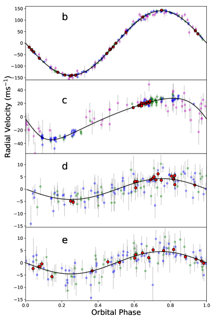
Figure 9: Phase-folded RVs with all GPs and systemic velocities removed for WASP-47 b (top), WASP-47 c (second), WASP-47 d (third), and WASP-47 e (bottom). The colors of the data from the various instruments are: ESPRESSO (red); HARPS-N (blue); HIRES (green); CORALIE (magenta). Note we do not plot the CORALIE data for planets d and e as the RMS of the CORALIE data is larger than the semi-amplitudes of these two planets.

3.7 Transit Timing Analysis

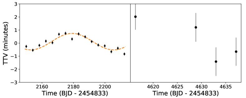
Figure 10: Observed TTVs for WASP-47 b for the transits in the Left: K2 photometry and Right: TESS photometry. The orange line gives the TTV model from Becker et al. (2015).

WASP-47 b and WASP-47 d have already been shown to exhibit significant transit timing variations (TTVs, eg. Becker et al., 2015; Weiss et al., 2017). Due to the low signal-to-noise of the TESS transits of these planets, we are unable to strongly constrain the transit center times for the individual TESS transits of WASP-47 d or WASP-47 e. However we can measure the transit times for the hot Jupiter WASP-47 b.

Epoch	Mid-Transit Time
	(BJD TDB)
587	2459449.35411 $\pm$ 0.00069
590	2459461.83099 $\pm$ 0.00076
591	2459465.98832 $\pm$ 0.00076
592	2459470.14800 $\pm$ 0.00075

Table 2: Measured TESS mid-transit times for WASP-47 b. The epoch is relative to the $T_{C}$ value given in Table 3.

We re-fit each transit of WASP-47 b in the TESS data in order to measure the individual $T_{C}$ values. During this analysis, we fix the transit shape to the model derived in Section 3.6. The same model is used to subtract the transits of WASP-47 d and WASP-47 e from the light curve before fitting. We also perform the same analysis for the WASP-47 b transits in the short cadence K2 data. The transit times measured are plotted in Figure 10 and provided in Table 2. The uncertainty on an individual $T_{C}$ from the TESS data is on the order of 1 minute, which is roughly twice the TTV amplitude seen in the K2 data. The TESS transit times display a scatter of a similar magnitude. As such, the $T_{C}$ measurements are consistent with the TTV predictions from the K2 results (see Figure 10). However the detection is marginal, and we cannot know the phase of the signal due to the significant time gap between K2 and TESS data.

4 Discussions

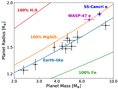
Figure 11: Mass-Radius diagram for low-mass exoplanets. The measurements and uncertainties are taken from the NASA exoplanet archive (accessed 2021 May 12). The black points show exoplanets with masses and radii measured to better than 10% precision. WASP-47 e is shown with the magenta star, and 55-Cancri e is plotted with the blue triangle. These two planets now have the most precise density measurements for any known super-Earths. The solid lines give various composition models from Zeng et al. (2016, 2019).

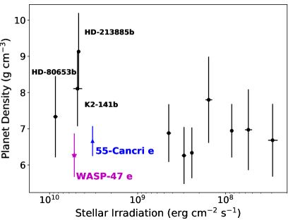
Figure 12: The variation of bulk planetary density with stellar irradiation for the sample of planets plotted in Figure 11. WASP-47 e is depicted by the magenta star and 55-Cancri e by the blue triangle.

The mass and density we measure for WASP-47 e are consistent at the 1$\sigma$ level with the results of Vanderburg et al. (2017). Vanderburg et al. (2017) use the planetary composition models of Lopez (2017) to show that their measured parameters of M_P = $6.83\pm 0.66$ M_⊕ and $\rho_{P}$ = $6.35\pm 0.64$ g cm^-3 are consistent with WASP-47 e having a steam-rich layer surrounding an Earth-like core and mantle. Due to the agreement between these measurements the the values derived in this work, such a composition remains a plausible scenario.

We compare our newly derived parameters for WASP-47 e to the sample of known planets with M_P $<10$ M_⊕, R_P $<2$ R_⊕ and mass and radius measurement precisions better than 10% (see Figure 11). We find that WASP-47 e is similar in mass and radius to 55-Cancri e, and that these two exoplanets are the only in the sample which onto the 100% MgSiO₃ composition model of Zeng et al. (2019). The WASP-47 and 55-Cancri planetary systems are also the only two to contain close in giant planets: WASP-47 b (M_P = $1.144\pm 0.023$ M_J; P = $4.159$ days) and 55-Cancri b (M_P = 0.804$\pm$0.009 M_J; P = 14.6516 days). WASP-47 e has a lower density than K2-141 b and HD-213885 b despite receiving a very similar amount of stellar irradiation (see Figure 12). 55-Cancri e receives a similar level of irradiation and has a similar density to WASP-47 e. It is possible that the presence of the close-in giant planet companions to these super-Earths has caused them to have a lower density than other planets with similar levels of stellar irradiation.

Due to the intense stellar irradiation, this reduced density is almost certainly not due to an extended H/He atmosphere because such an atmosphere would have been lost through photo-evaporation (Penz et al., 2008; Sanz-Forcada et al., 2011). One possibility could be the scenario with a steam-rich layer proposed by Vanderburg et al. (2017). Alternatively, Dorn et al. (2019) recently proposed that WASP-47 e and 55-Cancri e could have compositions rich in refractory elements, such as Ca and Al, which condense out of protoplanetary disks at high temperatures. This different elemental make-up was shown to result in planets with densities 10-20% less than a planet of the same R_P but with an Earth-like composition (Dorn et al., 2019) and therefore would explain the lower densities of these two planets, given the irradiation they receive.

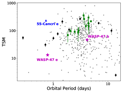
Figure 13: Comparison of TSM vs orbital period for various known exoplanets. We plot the sample of planets from the NASA Exoplanet Archive with a radius measured to better than 10% precision and a mass measured to better than 50% precision (grey points), the JWST community targets (green squares; Stevenson et al., 2016) and the sample of planets from Figure 11 (black points). WASP-47 b and WASP-47 e are depicted by the magenta stars and 55-Cancri e by the blue triangle.

Obtaining transmission spectroscopy observations for the three inner WASP-47 planets will provide further clues to unlock the formation history of this system. We use the transmission spectroscopy metric (TSM) from Kempton et al. (2018) to assess the potential for obtaining such observations. The TSM provides near-realistic values of the expected signal-to-noise ratio obtained from a 10 hr observation sequence with JWST. For the inner planets, we calculate values of $13.2\pm 1.3$ (WASP-47 e), $46.8\pm 2.3$ (WASP-47 b), and $23.4\pm 2.4$ (WASP-47 d). While modest compared to other planets with similar orbital parameters due to the relative faintness of WASP-47 (V = 11.94 mag) (see Figure 13), these values indicate that a significant amount of information on the atmospheric compositions of these planets can be achieved through JWST observations. Combined with the precise constraints on the masses of these planets, these atmospheric observations would provide great insight into the composition and possible formation history of the WASP-47 planets.

The potential detection of an atmosphere on 55-Cancri e has been reported from both HST (Tsiaras et al., 2016) and Spitzer (Angelo & Hu, 2017) observations. We also note that 55-Cancri e will be observed by JWST during its Cycle 1 observations. Due to the similarities between the two planets and their environments, any revelations about the atmospheric conditions of 55-Cancri e have implications for the likelihood of an atmosphere on WASP-47 e.

WASP-47 e and 55-Cancri e are the only two planets to fall solidly on the 100% MgSiO₃ composition line in Figure 11. This different composition of WASP-47 e and 55-Cancri e are possibly the result of these systems forming through a different pathway to the other planets shown. The nature of WASP-47 e orbiting interior to a hot Jupiter also strongly suggests a different planetary formation and evolution mechanism to the large majority of hot Jupiter systems (Huang et al., 2016). The formation of hot Earths and Neptunes interior to hot Jupiters can arise as a result of portions of the protoplanetary disk being shepherded to the inner regions of the planetary system by a giant planet migrating through disk interactions (Fogg & Nelson, 2005, 2007). This disk shepherding prior to the formation of WASP-47 e could provide a high temperature environment amenable to the formation from high temperature condensates (Dorn et al., 2019).

Poon et al. (2021) demonstrated that not only can an in-situ formation mechanism produce planetary systems containing hot Jupiters and inner small planets but also that this formation mechanism does not reproduce the observed population of single hot Jupiters. This again suggests that the WASP-47 planetary system formed through a different mechanism to other hot Jupiter systems. This scenario was also suggested by Huang et al. (2016), who note that the WASP-47 system bears stronger resemblance to the population of warm Jupiter systems, which often have smaller planets interior to the warm Jupiter. It is possible that the WASP-47 and 55-Cancri systems formed through a mechanism similar to warm Jupiter systems, resulting in different bulk compositions for WASP-47 e and 55-Cancri e.

With only two super-Earths with close giant planet companions and precisely measured densities, we do not have a large enough sample size from which to draw significant conclusions. A larger sample of known planets interior to hot Jupiters would allow us to better identify any trends in the properties of these inner companions. Therefore, further discoveries of small planets interior to hot and warm Jupiters are needed to shed light on how these systems form, and how the compositions the small planets are sculpted by their formation. There is a possibility that other known hot Jupiters have small planets orbiting interior to them. The majority of known transiting hot Jupiters were discovered by ground based transit surveys, and so the discovery data did not have sufficient photometric precision to detect super-Earth planets. WASP-47 d and WASP-47 e are only known thanks to the K2 data and of the 536 known exoplanets with $P<10$ days and M_P ¿ 0.1 M_J only 80 have received such high precision monitoring with Kepler or K2. It is therefore possible that several of the hot Jupiter host stars that have not been monitored at very high precision also contain inner transiting super-Earths interior to the orbits of their hot Jupiters.

The two stars WASP-47 and 55-Cancri have metallicities of [Fe/H]=$0.38\pm 0.05$ (Vanderburg et al., 2017) and [Fe/H]=$0.35\pm 0.10$ (Bourrier et al., 2018) respectively. These two stars are significantly more metal rich than the host stars for the other super-Earths in the sample considered in this paper (see Figure 14). While high metallicities are expected for stars which host close-in giant exoplanets (Fischer & Valenti, 2005), we find that WASP-47 and 55-Cancri have high metallicities even compared to the metallicity distribution for hot-Jupiter host stars. Osborn & Bayliss (2020) investigated this planet-metallicity correlation using a homogeneous sample of 217 hot Jupiter host stars. We find that WASP-47 is more metal rich than 96% of that sample, and 55-Cancri is more metal rich than 94%. It is possible that the high metallicity of the host stars has in some way affected the formation and composition of WASP-47 e and 55-Cancri e. However, we will only be able to confirm this correlation with the discovery of more small planets interior to close-in giant planets.

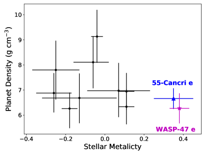
Figure 14: Planet bulk density plotted against stellar metallicity for WASP-47 e, 55-Cancri e, and the sample of super-Earths from Figure 11.

5 Conclusions

We report radial velocity measurements obtained for WASP-47 using the ESPRESSO spectrograph. We combined our new RV measurements with existing data obtained using the HARPS-N, HIRES and CORALIE spectrographs. Our measurements confirm that WASP-47 e is a super-Earth with a mass of $6.77\pm 0.57$ M_⊕ and a bulk density of $6.29\pm 0.60$ g cm^-3. Using these data, we improve the mass measurement precision for the super-Earth WASP-47 e and the Neptune-sized WASP-47 d by 15% and 13% respectively compared to the previous best measurements (Vanderburg et al., 2017). Our measured bulk density shows that WASP-47 e is similar in density, and likely composition, to 55-Cancri e. WASP-47 e has the second most precisely measured density of any super-Earth, only behind 55-Cancri e which orbits a much brighter host star.

We find variability in the K2 photometric data which is indicative of a $P_{\rm Rot}$ = 32.5$\pm$3.9 day rotation period for WASP-47. The improved precision of the ESPRESSO data compared to previous data sets allowed us to identify a stellar activity signal in the ESPRESSO radial velocity residuals and activity indicators with a periodicity consistent with the rotation period derived from K2.

With the inclusion of the TESS photometry, we refine the orbital ephemerides of the three inner planets. This refinement is vital for future follow-up observations. As an example, at the start of July 2022 when JWST observations should begin, our updated ephemeris predicts the transit of WASP-47 b to occur 20 minutes later than the older ephemeris of Becker et al. (2015). Our updated ephemeris has a 1$\sigma$ uncertainty of just 0.57 minutes, compared to 4.67 minutes from the older Becker et al. (2015) ephemeris. Similarly for WASP-47 d our new ephemeris predicts the transit to occur 114 minutes earlier, with a reduced 1$\sigma$ uncertainty of 35 minutes compared to 84 minutes. For WASP-47 e our new ephemeris predicts the transit to occur just 9.73 minutes earlier, but with a reduced 1$\sigma$ uncertainty of 25 minutes compared to 65 minutes. These refined transit predictions are crucial for properly planning and fully interpreting high value follow-up observations, such as transmission spectroscopy with JWST.

Due to the TESS photometry having a photometric precision of 3040 ppm-per-minute (c.f. K2 precision of 350 ppm-per-minute), the TESS data is unable to improve the constraints on the radii of the transiting planets. For similar reasons the TESS data is not sensitive to the stellar variability seen in the K2 data.

Compared to other well characterized super-Earths, WASP-47 e and 55-Cancri e stand out in terms of their low densities given their stellar environments and the presence of a close-orbiting giant planet. It is possible that a different formation mechanism to the majority of hot Jupiters was required to form these systems, and this difference in formation could have resulted in WASP-47 e and 55-Cancri e having different compositions to other super-Earths.

Table 3: Planetary parameters derived in this work in sections 3.1 and 3.6.

Parameter	Symbol	Unit	Prior	Value
Planetary parameters
WASP-47 e
Time of conjunction	$T_{C}$	BJD (TDB)	$\mathcal{N}\left(2457011.34863,0.00030\right)$	$2457011.34862\pm 0.00030$
Orbital Period	$P$	days	$\mathcal{N_{U}}\left(0.789595,0.000005,0.,\infty\right)$	$0.7895933\pm 0.0000044$
RV Semi-Amplitude	$K_{e}$	ms-1	$\mathcal{N_{U}}\left(5.,10.,0.,\infty\right)$	$4.55\pm 0.37$
Radius Ratio	$R_{e}/R_{*}$		$\mathcal{U}\left(0.,1.0\right)$	$0.01458\pm 0.00013$
Planet Mass†	$M_{e}$	M⊕		$6.77\pm 0.57$
Planet Radius†	$R_{e}$	R⊕		$1.808\pm 0.026$
Planet Density†	$\rho_{e}$	g cm-3		$6.29\pm 0.60$
WASP-47 b
Time of conjunction	$T_{C}$	BJD (TDB)	$\mathcal{N}\left(2457007.932103,0.000019\right)$	$2457007.932103\pm 0.000019$
Orbital Period	$P$	days	$\mathcal{N_{U}}\left(4.1591492,0.0000006,0.,\infty\right)$	$4.1591492\pm 0.0000006$
RV Semi-Amplitude	$K_{b}$	ms-1	$\mathcal{N_{U}}\left(150.,50.,0.,\infty\right)$	$140.84\pm 0.40$
Radius Ratio	$R_{b}/R_{*}$		$\mathcal{U}\left(0.,1.0\right)$	$0.10191\pm 0.00022$
Planet Mass†	$M_{b}$	M⊕		$363.6\pm 7.3$
Planet Radius†	$R_{b}$	R⊕		$12.64\pm 0.15$
Planet Density†	$\rho_{b}$	g cm-3		$0.989\pm 0.040$
WASP-47 d
Time of conjunction	$T_{C}$	BJD (TDB)	$\mathcal{N}\left(2457006.36955,0.00035\right)$	$2457006.36955\pm 0.00035$
Orbital Period	$P$	days	$\mathcal{N_{U}}\left(9.03055,0.0002,0.,\infty\right)$	$9.03055\pm 0.00008$
RV Semi-Amplitude	$K_{d}$	ms-1	$\mathcal{N_{U}}\left(5.,10.,0.,\infty\right)$	$4.26\pm 0.37$
Radius Ratio	$R_{d}/R_{*}$		$\mathcal{U}\left(0.,1.0\right)$	$0.02876\pm 0.00017$
Planet Mass†	$M_{d}$	M⊕		$14.2\pm 1.3$
Planet Radius†	$R_{d}$	R⊕		$3.567\pm 0.045$
Planet Density†	$\rho_{d}$	g cm-3		$1.72\pm 0.17$
Orbital Eccentricity	ed		$\mathcal{N_{U}}\left(0.,0.014,0.,1.\right)$	$0.010\,^{+0.011}_{-0.007}$
Argument of Periastron	$\omega_{d}$	deg	$\mathcal{U}\left(-180.,180.\right)$	$16.5\,^{+84.2}_{-98.6}$
WASP-47 c
Time of conjunction	$T_{C}$	BJD (TDB)	$\mathcal{N}\left(2457763.4,20.\right)$	$2457763.1\pm 4.3$
Orbital Period	$P$	days	$\mathcal{N_{U}}\left(590,15.,0.,\infty\right)$	$588.8\pm 2.0$
RV Semi-Amplitude	$K_{c}$	ms-1	$\mathcal{N_{U}}\left(30.,15.,0.,\infty\right)$	$31.04\pm 0.40$
Planet Minimum Mass†	$M_{c}\,\sin\,i$	M⊕		$398.9\pm 9.1$
Orbital Eccentricity	ec		$\mathcal{U}\left(0.,1.\right)$	$0.295\pm 0.016$
Argument of Periastron	$\omega_{c}$	deg	$\mathcal{U}\left(-180.,180.\right)$	$112.0\pm 4.3$

Table 4: Additional parameters from the sampling in Section 3.6.

Parameter	Unit	Prior	Value
Instrumental Parameters
$\gamma_{\rm ESP}$	ms-1	$\mathcal{U}\left(-27350.,-26850.\right)$	$-27165.95\pm 1.27$
$\gamma_{\rm HARPS}$	ms-1	$\mathcal{U}\left(-27350.,-26850.\right)$	$-27041.03\pm 0.55$
$\gamma_{\rm HIRES}$	ms-1	$\mathcal{U}\left(-250.,250.\right)$	$6.50\pm 0.75$
$\gamma_{\rm COR;A}$ †	ms-1	$\mathcal{U}\left(-27500.,-26500.\right)$	$-27081.33\pm 1.89$
$\gamma_{\rm COR;B}$ †	ms-1	$\mathcal{U}\left(-27500.,-26500.\right)$	$-27067.57\pm 5.96$
$\gamma_{\rm ESPFWHM}$	ms-1	$\mathcal{U}\left(7600.,7700.\right)$	$7635.6\pm 1.0$
$\log_{10}\,\sigma_{\rm ESP}$	$\log\,$ms-1	$\mathcal{U}\left(-5.,1.\right)$	$0.145\pm 0.214$
$\log_{10}\,\sigma_{\rm HARPS}$	$\log\,$ms-1	$\mathcal{U}\left(-5.,1.\right)$	$-2.33\pm 1.82$
$\log_{10}\,\sigma_{\rm HIRES}$	$\log\,$ms-1	$\mathcal{U}\left(-5.,1.\right)$	$0.488\pm 0.069$
$\log_{10}\,\sigma_{\rm COR;A}$ †	$\log\,$ms-1	$\mathcal{U}\left(-7.,2.\right)$	$-2.38\pm 3.03$
$\log_{10}\,\sigma_{\rm COR;B}$ †	$\log\,$ms-1	$\mathcal{U}\left(-7.,2.\right)$	$-2.95\pm 2.75$
$\log_{10}\,\sigma_{\rm ESPFWHM}$	$\log\,$ms-1	$\mathcal{U}\left(-7.,1.\right)$	$-2.79\pm 0.13$
GP Hyperparameters
$P_{\rm Rot}$	days	$\mathcal{N_{U}}\left(35,10,28,\infty\right)$	$39.4\,^{+2.2}_{-4.5}$
$\ln\,Q$		$\mathcal{U}\left(1.15,15\right)$	$2.6\,^{+5.2}_{-1.1}$
$\ln\,\Delta\,Q$		$\mathcal{U}\left(-7,10\right)$	$-0.40\,^{+6.18}_{-5.04}$
$f$		$\mathcal{U}\left(0,1\right)$	$0.52\,^{+0.32}_{-0.31}$
$\sigma_{\rm GP,ESP}$		$\mathcal{U}\left(0,20\right)$	$4.58\,^{+3.83}_{-2.44}$
$\sigma_{\rm GP,ESPFWHM}$		$\mathcal{U}\left(0,100\right)$	$7.04\,^{+4.18}_{-2.16}$

Data Availability

The observations made with ESPRESSO (program 0103.C-0422) are publicly available through the ESO archive (http://archive.eso.org/) and the reduced radial-velocities are available in Table 5. The K2-SFF long cadence photometry is available as a High Level Science Product through the MAST database (https://archive.stsci.edu/hlsp/k2sff), and the short candence light curve is available for download from http://www.cfa.harvard.edu/ avanderb/wasp47sc.csv. The archival radial velocity measurements used were accessed and are available through the online versions of the corresponding publications: HARPS-N (Vanderburg et al., 2017); HIRES (Sinukoff et al., 2017); CORALIE (Neveu-VanMalle et al., 2016); PFS (Dai et al., 2015).

Appendix A ESPRESSO Radial-Velocities

Table 5: ESPRESSO radial-velocities of WASP-47.

Time	RV	RV err	CCF FWHM	CCF FWHM err	CCF Contrast	CCF Contrast err
(BJD)	kms-1	kms-1	kms-1	kms-1	%	%
2458701.85502825	-27.29026780	0.00041693	7.63531365	0.00083385	67.60791253	0.00738344
2458719.64853384	-27.09946692	0.00040187	7.63677533	0.00080374	67.56452335	0.00711092
2458721.58500371	-27.16635045	0.00049575	7.63476836	0.00099150	67.64179346	0.00878440
†2458725.61367832	-27.13500443	0.00065487	7.62975492	0.00130973	67.63890353	0.01161098
†2458725.63068667	-27.13984263	0.00062360	7.63615268	0.00124719	67.57960736	0.01103759
†2458725.64619095	-27.14989021	0.00094470	7.64294765	0.00188939	67.57891409	0.01670599
2458727.61484710	-27.16918161	0.00059743	7.63368748	0.00119485	67.62341354	0.01058467
2458727.67178015	-27.15824555	0.00065289	7.63523000	0.00130578	67.62855131	0.01156585
2458727.73682302	-27.14140987	0.00058531	7.63690880	0.00117061	67.61934501	0.01036494
2458728.78485747	-27.00354831	0.00045830	7.63894339	0.00091660	67.57051680	0.00810783
2458729.56054875	-27.09212322	0.00044374	7.63200749	0.00088747	67.59110555	0.00785971
2458729.61834544	-27.10772602	0.00090117	7.63388129	0.00180233	67.68960271	0.01598127
2458736.67233204	-27.03578795	0.00061549	7.62430696	0.00123098	67.32722849	0.01087029
∗2458740.75353437	-27.05016571	0.00062895	7.57708547	0.00125790	65.82775520	0.01092832
∗2458740.77067861	-27.04230379	0.00078360	7.54293260	0.00156719	64.96525397	0.01349782
2458742.61293777	-27.21117435	0.00043227	7.63387461	0.00086453	67.34888424	0.00762724
†2458746.53807873	-27.15209672	0.00044709	7.64715905	0.00089417	67.20359011	0.00785802
2458746.59477314	-27.16215262	0.00044244	7.64505752	0.00088487	67.30934962	0.00779069
2458746.64130096	-27.17045794	0.00043855	7.64196106	0.00087710	67.38690784	0.00773431
2458747.52008568	-27.27233326	0.00050739	7.64561227	0.00101477	67.49901637	0.00895886
2458751.51960422	-27.28267043	0.00048916	7.64547970	0.00097833	67.52486603	0.00864059
2458751.64509613	-27.29039615	0.00045045	7.64359568	0.00090089	67.50749933	0.00795661
2458755.51389449	-27.26383303	0.00048269	7.63960650	0.00096538	67.57048540	0.00853854
2458756.64036787	-27.18625399	0.00044636	7.63636160	0.00089273	67.64158456	0.00790762
2458756.70863783	-27.16868373	0.00045565	7.63589503	0.00091131	67.63068642	0.00807142

• $\dagger$ Data points taken during a transit of WASP-47 b and so excluded from analysis

• * Data points excluded from analysis due to anomalous CCF profiles

References

- Almenara et al. (2016) Almenara, J. M., Díaz, R. F., Bonfils, X., & Udry, S. 2016, A&A, 595, L5, doi: 10.1051/0004-6361/201629770
- Angelo & Hu (2017) Angelo, I., & Hu, R. 2017, AJ, 154, 232, doi: 10.3847/1538-3881/aa9278
- Astropy Collaboration et al. (2013) Astropy Collaboration, Robitaille, T. P., Tollerud, E. J., et al. 2013, A&A, 558, A33, doi: 10.1051/0004-6361/201322068
- Astropy Collaboration et al. (2018) Astropy Collaboration, Price-Whelan, A. M., Sipőcz, B. M., et al. 2018, AJ, 156, 123, doi: 10.3847/1538-3881/aabc4f
- Barnes (2007) Barnes, S. A. 2007, ApJ, 669, 1167, doi: 10.1086/519295
- Becker et al. (2015) Becker, J. C., Vanderburg, A., Adams, F. C., Rappaport, S. A., & Schwengeler, H. M. 2015, ApJ, 812, L18, doi: 10.1088/2041-8205/812/2/L18
- Boisse et al. (2011) Boisse, I., Bouchy, F., Hébrard, G., et al. 2011, A&A, 528, A4, doi: 10.1051/0004-6361/201014354
- Borucki et al. (2010) Borucki, W. J., Koch, D., Basri, G., et al. 2010, Science, 327, 977, doi: 10.1126/science.1185402
- Bourrier et al. (2018) Bourrier, V., Dumusque, X., Dorn, C., et al. 2018, A&A, 619, A1, doi: 10.1051/0004-6361/201833154
- Cañas et al. (2019) Cañas, C. I., Wang, S., Mahadevan, S., et al. 2019, ApJ, 870, L17, doi: 10.3847/2041-8213/aafa1e
- Chatterjee et al. (2008) Chatterjee, S., Ford, E. B., Matsumura, S., & Rasio, F. A. 2008, ApJ, 686, 580, doi: 10.1086/590227
- Clarke (2003) Clarke, D. 2003, A&A, 407, 1029, doi: 10.1051/0004-6361:20030901
- Dai et al. (2015) Dai, F., Winn, J. N., Arriagada, P., et al. 2015, ApJ, 813, L9, doi: 10.1088/2041-8205/813/1/L9
- Dawson & Johnson (2018) Dawson, R. I., & Johnson, J. A. 2018, ARA&A, 56, 175, doi: 10.1146/annurev-astro-081817-051853
- Demory et al. (2012) Demory, B.-O., Gillon, M., Seager, S., et al. 2012, ApJ, 751, L28, doi: 10.1088/2041-8205/751/2/L28
- Donahue et al. (1997) Donahue, R. A., Dobson, A. K., & Baliunas, S. L. 1997, Sol. Phys., 171, 191, doi: 10.1023/A:1004902307998
- Dorn et al. (2019) Dorn, C., Harrison, J. H. D., Bonsor, A., & Hands, T. O. 2019, MNRAS, 484, 712, doi: 10.1093/mnras/sty3435
- Dreizler et al. (2020) Dreizler, S., Crossfield, I. J. M., Kossakowski, D., et al. 2020, A&A, 644, A127, doi: 10.1051/0004-6361/202038016
- Fischer & Valenti (2005) Fischer, D. A., & Valenti, J. 2005, ApJ, 622, 1102, doi: 10.1086/428383
- Fogg & Nelson (2005) Fogg, M. J., & Nelson, R. P. 2005, A&A, 441, 791, doi: 10.1051/0004-6361:20053453
- Fogg & Nelson (2007) —. 2007, A&A, 472, 1003, doi: 10.1051/0004-6361:20077950
- Foreman-Mackey (2018a) Foreman-Mackey, D. 2018a, Research Notes of the American Astronomical Society, 2, 31, doi: 10.3847/2515-5172/aaaf6c
- Foreman-Mackey (2018b) —. 2018b, Research Notes of the American Astronomical Society, 2, 31, doi: 10.3847/2515-5172/aaaf6c
- Foreman-Mackey et al. (2017a) Foreman-Mackey, D., Agol, E., Ambikasaran, S., & Angus, R. 2017a, AJ, 154, 220, doi: 10.3847/1538-3881/aa9332
- Foreman-Mackey et al. (2017b) —. 2017b, AJ, 154, 220, doi: 10.3847/1538-3881/aa9332
- Foreman-Mackey et al. (2013) Foreman-Mackey, D., Hogg, D. W., Lang, D., & Goodman, J. 2013, PASP, 125, 306, doi: 10.1086/670067
- Foreman-Mackey et al. (2020) Foreman-Mackey, D., Luger, R., Czekala, I., et al. 2020, exoplanet-dev/exoplanet v0.3.2, doi: 10.5281/zenodo.1998447
- Freudling et al. (2013) Freudling, W., Romaniello, M., Bramich, D. M., et al. 2013, A&A, 559, A96, doi: 10.1051/0004-6361/201322494
- Gaia Collaboration et al. (2021) Gaia Collaboration, Brown, A. G. A., Vallenari, A., et al. 2021, A&A, 649, A1, doi: 10.1051/0004-6361/202039657
- Gelman & Rubin (1992) Gelman, A., & Rubin, D. B. 1992, Statistical Science, 7, 457, doi: 10.1214/ss/1177011136
- Hellier et al. (2012) Hellier, C., Anderson, D. R., Collier Cameron, A., et al. 2012, MNRAS, 426, 739, doi: 10.1111/j.1365-2966.2012.21780.x
- Howell et al. (2014) Howell, S. B., Sobeck, C., Haas, M., et al. 2014, PASP, 126, 398, doi: 10.1086/676406
- Huang et al. (2016) Huang, C., Wu, Y., & Triaud, A. H. M. J. 2016, ApJ, 825, 98, doi: 10.3847/0004-637X/825/2/98
- Huang et al. (2020) Huang, C. X., Quinn, S. N., Vanderburg, A., et al. 2020, ApJ, 892, L7, doi: 10.3847/2041-8213/ab7302
- Jenkins et al. (2016) Jenkins, J. M., Twicken, J. D., McCauliff, S., et al. 2016, in Society of Photo-Optical Instrumentation Engineers (SPIE) Conference Series, Vol. 9913, Software and Cyberinfrastructure for Astronomy IV, ed. G. Chiozzi & J. C. Guzman, 99133E, doi: 10.1117/12.2233418
- Kempton et al. (2018) Kempton, E. M. R., Bean, J. L., Louie, D. R., et al. 2018, PASP, 130, 114401, doi: 10.1088/1538-3873/aadf6f
- Kipping (2013) Kipping, D. M. 2013, MNRAS, 435, 2152, doi: 10.1093/mnras/stt1435
- Knutson et al. (2014) Knutson, H. A., Fulton, B. J., Montet, B. T., et al. 2014, ApJ, 785, 126, doi: 10.1088/0004-637X/785/2/126
- Kosiarek & Crossfield (2020) Kosiarek, M. R., & Crossfield, I. J. M. 2020, AJ, 159, 271, doi: 10.3847/1538-3881/ab8d3a
- Kovács et al. (2002) Kovács, G., Zucker, S., & Mazeh, T. 2002, A&A, 391, 369, doi: 10.1051/0004-6361:20020802
- Kozai (1962) Kozai, Y. 1962, AJ, 67, 591, doi: 10.1086/108790
- Kreidberg (2015) Kreidberg, L. 2015, PASP, 127, 1161, doi: 10.1086/683602
- Leleu et al. (2021) Leleu, A., Alibert, Y., Hara, N. C., et al. 2021, A&A, 649, A26, doi: 10.1051/0004-6361/202039767
- Lidov (1962) Lidov, M. L. 1962, Planet. Space Sci., 9, 719, doi: 10.1016/0032-0633(62)90129-0
- Lillo-Box et al. (2020) Lillo-Box, J., Figueira, P., Leleu, A., et al. 2020, A&A, 642, A121, doi: 10.1051/0004-6361/202038922
- Lin et al. (1996) Lin, D. N. C., Bodenheimer, P., & Richardson, D. C. 1996, Nature, 380, 606, doi: 10.1038/380606a0
- Lopez (2017) Lopez, E. D. 2017, MNRAS, 472, 245, doi: 10.1093/mnras/stx1558
- McQuillan et al. (2013) McQuillan, A., Aigrain, S., & Mazeh, T. 2013, MNRAS, 432, 1203, doi: 10.1093/mnras/stt536
- Mustill et al. (2015) Mustill, A. J., Davies, M. B., & Johansen, A. 2015, ApJ, 808, 14, doi: 10.1088/0004-637X/808/1/14
- Neath & Cavanaugh (2012) Neath, A. A., & Cavanaugh, J. E. 2012, WIREs Computational Statistics, 4, 199, doi: https://doi.org/10.1002/wics.199
- Nelson et al. (2000) Nelson, R. P., Papaloizou, J. C. B., Masset, F., & Kley, W. 2000, MNRAS, 318, 18, doi: 10.1046/j.1365-8711.2000.03605.x
- Neveu-VanMalle et al. (2016) Neveu-VanMalle, M., Queloz, D., Anderson, D. R., et al. 2016, A&A, 586, A93, doi: 10.1051/0004-6361/201526965
- Osborn & Bayliss (2020) Osborn, A., & Bayliss, D. 2020, MNRAS, 491, 4481, doi: 10.1093/mnras/stz3207
- Osborn et al. (2021) Osborn, H. P., Armstrong, D. J., Adibekyan, V., et al. 2021, MNRAS, 502, 4842, doi: 10.1093/mnras/stab182
- Oshagh et al. (2017) Oshagh, M., Santos, N. C., Figueira, P., et al. 2017, A&A, 606, A107, doi: 10.1051/0004-6361/201731139
- Papaloizou & Larwood (2000) Papaloizou, J. C. B., & Larwood, J. D. 2000, MNRAS, 315, 823, doi: 10.1046/j.1365-8711.2000.03466.x
- Penz et al. (2008) Penz, T., Micela, G., & Lammer, H. 2008, A&A, 477, 309, doi: 10.1051/0004-6361:20078364
- Pepe et al. (2020) Pepe, F., Cristiani, S., Rebolo, R., et al. 2020, arXiv e-prints, arXiv:2010.00316. https://arxiv.org/abs/2010.00316
- Poon et al. (2021) Poon, S. T. S., Nelson, R. P., & Coleman, G. A. L. 2021, arXiv e-prints, arXiv:2105.08553. https://arxiv.org/abs/2105.08553
- Ricker et al. (2014) Ricker, G. R., Winn, J. N., Vanderspek, R., et al. 2014, in Society of Photo-Optical Instrumentation Engineers (SPIE) Conference Series, Vol. 9143, Space Telescopes and Instrumentation 2014: Optical, Infrared, and Millimeter Wave, ed. J. Oschmann, Jacobus M., M. Clampin, G. G. Fazio, & H. A. MacEwen, 914320, doi: 10.1117/12.2063489
- Salvatier et al. (2016) Salvatier, J., Wiecki, T. V., & Fonnesbeck, C. 2016, PeerJ Computer Science, 2, e55
- Sanchis-Ojeda et al. (2015) Sanchis-Ojeda, R., Winn, J. N., Dai, F., et al. 2015, ApJ, 812, L11, doi: 10.1088/2041-8205/812/1/L11
- Sanz-Forcada et al. (2011) Sanz-Forcada, J., Micela, G., Ribas, I., et al. 2011, A&A, 532, A6, doi: 10.1051/0004-6361/201116594
- Schwarz (1978) Schwarz, G. 1978, Annals of Statistics, 6, 461
- Shan et al. (2021) Shan, S.-S., Yang, F., Lu, Y.-J., et al. 2021, arXiv e-prints, arXiv:2111.06678. https://arxiv.org/abs/2111.06678
- Sinukoff et al. (2017) Sinukoff, E., Howard, A. W., Petigura, E. A., et al. 2017, AJ, 153, 70, doi: 10.3847/1538-3881/153/2/70
- Skrutskie et al. (2006) Skrutskie, M. F., Cutri, R. M., Stiening, R., et al. 2006, AJ, 131, 1163, doi: 10.1086/498708
- Sozzetti et al. (2021) Sozzetti, A., Damasso, M., Bonomo, A. S., et al. 2021, A&A, 648, A75, doi: 10.1051/0004-6361/202040034
- Stassun et al. (2019) Stassun, K. G., Oelkers, R. J., Paegert, M., et al. 2019, AJ, 158, 138, doi: 10.3847/1538-3881/ab3467
- Steffen et al. (2012) Steffen, J. H., Ragozzine, D., Fabrycky, D. C., et al. 2012, Proceedings of the National Academy of Science, 109, 7982, doi: 10.1073/pnas.1120970109
- Stevenson et al. (2016) Stevenson, K. B., Lewis, N. K., Bean, J. L., et al. 2016, PASP, 128, 094401, doi: 10.1088/1538-3873/128/967/094401
- Theano Development Team (2016) Theano Development Team. 2016, arXiv e-prints, abs/1605.02688. http://arxiv.org/abs/1605.02688
- Tsiaras et al. (2016) Tsiaras, A., Rocchetto, M., Waldmann, I. P., et al. 2016, ApJ, 820, 99, doi: 10.3847/0004-637X/820/2/99
- Vanderburg & Johnson (2014) Vanderburg, A., & Johnson, J. A. 2014, PASP, 126, 948, doi: 10.1086/678764
- Vanderburg et al. (2015) Vanderburg, A., Montet, B. T., Johnson, J. A., et al. 2015, 800, 59, doi: 10.1088/0004-637x/800/1/59
- Vanderburg et al. (2017) Vanderburg, A., Becker, J. C., Buchhave, L. A., et al. 2017, AJ, 154, 237, doi: 10.3847/1538-3881/aa918b
- Weiss et al. (2017) Weiss, L. M., Deck, K. M., Sinukoff, E., et al. 2017, AJ, 153, 265, doi: 10.3847/1538-3881/aa6c29
- Zeng et al. (2016) Zeng, L., Sasselov, D. D., & Jacobsen, S. B. 2016, ApJ, 819, 127, doi: 10.3847/0004-637X/819/2/127
- Zeng et al. (2019) Zeng, L., Jacobsen, S. B., Sasselov, D. D., et al. 2019, Proceedings of the National Academy of Science, 116, 9723, doi: 10.1073/pnas.1812905116