Counting flags of primitive lattices

?abstractname?

We count flags of primitive lattices, which are objects of the form $\left\{0\right\}=\Lambda^{(0)}<\Lambda^{(1)}<\cdots<\Lambda^{(\ell)}=\mathbb{Z}^{n}$, where every $\Lambda^{(i)}$ is a primitive lattice in $\mathbb{Z}^{n}$. The counting is with respect to two different natural height functions, allowing us to give a new proof of the Manin conjecture for flag varieties over the rational numbers. We deduce the equidistribution of rational points in flag varieties, as well as the equidistribution of the shapes of the successive quotient lattices $\Lambda^{(i)}/\Lambda^{(i-1)}$. In doing so, we generalize previous work of Schmidt, as well as our own, on counting primitive lattices of rank $d<n$.

1 Introduction

Let $n>1$ and let $\underline{d}=(d_{1},\ldots d_{\ell})$ be a partition of $n$, namely an $\ell$-tuple of (strictly) positive integers such that $d_{1}+\cdots+d_{\ell}=n$. Consider a flag of subspaces of $\mathbb{R}^{n}$,

$$\mathbf{F}=\>(\,\left\{0\right\}=V_{0}<V_{1}<\cdots<V_{\ell}=\mathbb{R}^{n}\,),$$ (1.1)

with $\dim(V_{i})=d_{1}+\cdots+d_{i}$ for all $1\leq 1\leq n$. If all the subspaces $V_{i}$ are rational (that is, have a basis consisting of rational vectors), then each contains a unique primitive lattice of rank $\dim(V_{i})$,

$$\Lambda^{(i)}=V_{i}\cap\mathbb{Z}^{n},$$

and we obtain a flag of primitive lattices

$$\mathbf{F}(\mathbb{Z})=\;(\,\left\{0\right\}=\Lambda^{(0)}<\Lambda^{(1)}<\cdots<\Lambda^{(\ell)}=\mathbb{Z}^{n}\,).$$ (1.2)

The aim of this paper is to extend known counting and equidistribution results from primitive lattices to flags of primitive lattices. Schmidt [Sch68, Thm. 1] was the first to prove a counting result for primitive lattices of rank $1\leq d\leq n$ in $\mathbb{R}^{n}$, showing that the number of primitive lattices of rank $d$ with covolume up to $X$ is

$$c_{d,n}X^{n}+O(X^{n-\max\{\frac{1}{d},\frac{1}{n-d}\}}),$$ (1.3)

where the covolume of a lattice is the volume of a fundamental parallelepiped for the lattice in the linear space it spans and

$$c_{d,n}=\frac{1}{n}{n\choose d}\frac{\zeta(2)\cdots\zeta(d)}{\zeta(n-d+1)\cdots\zeta(n)}\frac{\mathfrak{V}(n-d+1)\cdots\mathfrak{V}(n)}{\mathfrak{V}(1)\cdots\mathfrak{V}(d)};$$ (1.4)

here $\zeta$ is the Riemann Zeta function and $\mathfrak{V}(i)$ is the Lebesgue volume of the a ball in $\mathbb{R}^{i}$. (This result was generalized to general number fields by Thunder [Thu92, Thm. 1], who also proved a counting result [Thu93, Thm. 3] for primitive $d$-lattices that do not intersect a certain $(n-d)$-dimensional subspace. The error term in (1.3) was distilled by Kim [Kim19, Thm. 1.3]). Later, Schmidt [Sch98, Thm. 2] refined (1.3) so that it also takes into account the shape of the lattices, where the shape of a lattice in $\mathbb{R}^{n}$ is its equivalence class modulo rotation in $\mathbb{R}^{n}$ and rescaling by a positive scalar. The space of shapes of rank $d$ lattices is denoted by $\mathcal{X}_{d}$ (to be defined explicitly in Section 2); it is not compact, but it admits a natural uniform probability measure, $\mbox{vol}_{\mathcal{X}_{d}}^{1}$. Schmidt showed that given a Jordan measurable subset $\mathcal{E}\subset\mathcal{X}_{d}$, the number of primitive lattices with covolume up to $X$ and shape inside $\mathcal{E}$ is

$$\sim c_{d,n}\cdot\mbox{vol}_{\mathcal{X}_{d}}^{1}(\mathcal{E})X^{n}.$$

Since the subsets $\mathcal{E}$ are general enough, this counting can be read as an equidistribution statement, namely that the shapes of primitive lattices equidistribute in $\mathcal{X}_{d}$ as their covolume tends to infinity.

Dynamical techniques opened the door to equidistribution theorems that do not follow from (nor imply) counting statements, but with the advantage of considering lattices of covolume exactly $X$ (as apposed to at most $X$). Primarily, the focus was on the case $d=n-1$, namely on primitive lattices that lie in hyperplanes defined by being orthogonal to primitive vectors. Such equidistribution results were established by Aka, Einsiedler and Shapira [AES16a, AES16b], Einsiedler, Mozes, Shah and Shapira [EMSS16], and (with a bound on the rate of convergence) by Einsiedler, Rï¿œhr and Wirth [ERW17]. In fact, these equidistribution results were joint for the shapes of the primitive lattices in $\mathcal{X}_{n-1}$, and the projections of the primitive vectors orthogonal to these lattices to the unit sphere in $\mathbb{R}^{n}$ — in other words, for shapes of primitive $(n-1)$-lattices, and their directions. For general $d$, the direction of a $d$-lattice $\Lambda$ is the real linear space that it spans,

$$V_{\Lambda}=\mbox{span}_{\mathbb{R}}(\Lambda),$$

lying in the Grassmannian $\operatorname{Gr}^{0}(d,n)$ of $d$-dimesional subspaces of $\mathbb{R}^{n}$. In [Sch15, Thm. 1.2], Schmidt showed that for quite restricted types of sets $\mathcal{E}\subset\mathcal{X}_{d}$ and $\Phi\subseteq\operatorname{Gr}^{0}(d,n)$, the number of primitive $d$-lattices with shapes in $\mathcal{E}$ and directions in $\Phi$ is

$$c_{d,n}\cdot\mbox{vol}_{\mathcal{X}_{d}}^{1}(\mathcal{E})\mbox{vol}_{\operatorname{Gr}^{0}(d,n)}^{1}(\Phi)X^{n}+O(X^{n-\frac{1}{d}}\cdot\log^{d-1}X),$$

where $\mbox{vol}_{\operatorname{Gr}^{0}(d,n)}^{1}$ is the uniform probability measure on $\operatorname{Gr}^{0}(d,n)$. In [HK20a], we were able to extend the above result to subsets $\mathcal{E}$ and $\Phi$ that were general enough to conclude equidistribution, as well as to consider the orthogonal lattices

$$\Lambda^{\perp}=\mathbb{Z}^{n}\cap V_{\Lambda}^{\perp}$$

to primitive lattices $\Lambda$, where $V_{\Lambda}^{\perp}$ is the orthogonal complement of $V_{\Lambda}$ in $\mathbb{R}^{n}$. The consideration of the orthogonal lattices proved to be crucial in an application to the study of rational points on Grassmannians, described below. Finally, Aka, Musso and Wieser [AMW21] have extended the aforementioned equidistribution results on shapes of primitive lattices with covolume $X$, from rank $n-1$ to a general rank.

Our goal in the present paper is to generalize the counting result in [HK20a] from primitive lattices to flags of such. To this end, for $\underline{d}=(d_{1},\ldots d_{\ell})$ as above, we let

$$\operatorname{Gr}^{0}(\underline{d},n)=\text{space of $\underline{d}$-flags in $\mathbb{R}^{n}$}$$ (1.5)

(a $\underline{d}$-flag is the object defined in (1.1)), and

$$\mathcal{X}_{\underline{d}}=\prod_{i=1}^{\ell}\mathcal{X}_{d_{i}}\,.$$ (1.6)

Notice that one cannot expect equidistribution of the projections of $\Lambda^{(i)}$ to $\mathcal{X}_{d_{1}+\cdots+d_{i}}$ or to $\operatorname{Gr}^{0}(d_{i},n)$ jointly for all $i=1,\ldots,n$, since the relation of inclusion between the $\Lambda^{(i)}$’s implies dependence. Instead, we consider the successive quotients:

$$L_{1}=\Lambda^{(1)}/\Lambda^{(0)}\,,\ldots,\,L_{\ell}=\Lambda^{(\ell)}/\Lambda^{(\ell-1)},$$

where we note that $\operatorname{rank}(L_{i})=d_{i}$ for all $1\leq i\leq\ell$. Let

$$\operatorname{shape}\left(\mathbf{F}(\mathbb{Z})\right)=\left(\operatorname{shape}\left(L_{1}\right),\ldots,\operatorname{shape}\left(L_{\ell}\right)\right)\in\mathcal{X}_{\underline{d}}\,.$$

(As explained in Section 2, the quotients $L_{i}$ are isometric to concrete lattices in $\mathbb{R}^{n}$, so their shapes are well defined). Our first counting result is with respect to the height function

$$H_{\infty}(\mathbf{F}(\mathbb{Z}))=\max\{\operatorname{covol}(\Lambda^{(1)}),\ldots,\operatorname{covol}(\Lambda^{(\ell)})\}.$$

A subset of an orbifold is called boundary controllable [HK20b, Def. 1.2] if its boundary satisfies a standard regularity condition (Definition 4.2).

Theorem 1.1.

Let $\mathcal{E}\subseteq\mathcal{X}_{\underline{d}}$ and $\Phi\subseteq\operatorname{Gr}^{0}(\underline{d},n)$ be boundary controllable. The number of primitive lattice $\underline{d}$-flags $\mathbf{F}(\mathbb{Z})$ with $H_{\infty}(\mathbf{F}(\mathbb{Z}))\leq X$, $\mathbf{F}\in\Phi$ and $\operatorname{shape}\left(\mathbf{F}(\mathbb{Z})\right)\in\mathcal{E}$ is

$$c_{\underline{d},n}\cdot\mbox{vol}_{\mathcal{X}_{\underline{d}}}^{1}(\mathcal{E})\mbox{vol}_{\operatorname{Gr}^{0}(\underline{d},n)}^{1}(\Phi)\cdot X^{2n-d_{1}-d_{\ell}}+O_{\epsilon}(X^{(2n-d_{1}-d_{\ell})\left(1-\frac{1}{16n^{2}}+\epsilon\right)})$$

for all $\epsilon>0$, where

$$c_{\underline{d},n}=\frac{1}{2^{\ell-1}}\frac{1}{\prod_{i=1}^{\ell-1}(d_{i}+d_{i+1})}{n\choose d_{1},\ldots,d_{\ell}}\frac{\prod_{i=1}^{\ell-1}\prod_{j=2}^{d_{i}}\zeta(j)}{\prod_{i=2}^{d_{\ell}}\zeta\left(i\right)}\frac{\prod_{i=d_{\ell}+1}^{n}\mathfrak{V}(i)}{\prod_{i=1}^{\ell-1}\prod_{j=1}^{d_{i}}\mathfrak{V}(j)}.$$ (1.7)

Notice that when $\ell=2$, the lattice flag $\mathbf{F}(\mathbb{Z})$ is in fact a single primitive lattice $\Lambda<\mathbb{Z}^{n}$, and then the constant $c_{\underline{d},n}$ coincides with Schmidt’s constant (1.4). Indeed, returning to Schmidt’s result on primitive lattices, the one to one correspondence between primitive $d$-lattices in $\mathbb{Z}^{n}$ and rational $d$-dimensional subspaces of $\mathbb{R}^{n}$ ($V\mapsto V\cap\mathbb{Z}^{n}$ and $V_{\Lambda}\mapsfrom\Lambda$) means that the primitive $d$-lattices are in fact the rational points on the projective variety $\operatorname{Gr}^{0}(d,n)$. Since the anticanonical height function on this variety is

$$H_{\operatorname{ac}}(V_{\Lambda})=\operatorname{covol}(\Lambda)^{n},$$

then (1.3) can be read as one on counting rational points on the Grassmannian w.r.t. the anticanonical height function, and in particular it confirms Manin’s Conjecture [FMT89, Pey95] for this variety. The anticanonical height function on the flag variety $\operatorname{Gr}^{0}(\underline{d},n)$ (whose elements are $\underline{d}$-flags of the form (1.1), and whose rational points are primitive lattice $\underline{d}$-flags as in (1.2)) is

$$H_{\operatorname{ac}}(\mathbf{F}(\mathbb{Z}))=\prod_{i=0}^{\ell-1}\operatorname{covol}(\Lambda^{(i)})^{d_{i}+d_{i+1}}$$

[Pap83, Thu93], and it is known by the work of Franke, Manin and Tschinkel [FMT89, Cor. from Thm. 5] that flag varieties also satisfy Manin’s conjecture (see also [Thu93, Thm. 5] and [Kim19, Cor. 1.3] for the special case of flags in which $\Lambda^{(1)}$ intersects trivially a given subspace). However, just as (1.3) can be refined to include the shapes and directions of primitive lattices, so can the counting of primitive lattice flags. Our second result is on counting primitive lattice flags with respect to the height function $H_{\operatorname{ac}}$, and with consideration of shapes and directions.

Theorem 1.2.

Let $\mathcal{E}\subseteq\mathcal{X}_{\underline{d}}$ and $\Phi\subseteq\operatorname{Gr}^{0}(\underline{d},n)$ be boundary controllable. The number of primitive lattice $\underline{d}$-flags $\mathbf{F}(\mathbb{Z})$ with $H_{\operatorname{ac}}(\mathbf{F}(\mathbb{Z}))\leq X$, $\mathbf{F}\in\Phi$ and $\operatorname{shape}\left(\mathbf{F}(\mathbb{Z})\right)\in\mathcal{E}$ is

$$c_{\underline{d},n}\cdot\mbox{vol}_{\mathcal{X}_{\underline{d}}}^{1}(\mathcal{E})\mbox{vol}_{\operatorname{Gr}^{0}(\underline{d},n)}^{1}(\Phi)\cdot X\sum_{j=0}^{\ell-2}\frac{(-1)^{\ell-2-j}}{j!}(\log X)^{j}+O_{\epsilon}(X^{\left(1-\frac{1}{16n^{2}}+\epsilon\right)})$$

for all $\epsilon>0$, where $c_{\underline{d},n}$ is as in (1.7).

The refinement of Franke, Manin and Tschinkel’s result suggested in Theorem 1.2 could prove useful in further study of rational points on flag varieties: Browning, the first author and Wilsch [BHW21] built on [HK20a] to establish the freeness variant of Manin’s conjecture, proposed by Peyre [Pey17, Pey18], for Grassmannians. We expect that Theorem 1.2 could be used to extend the results in [BHW21] from Grassmannians to more general flag varieties.

Organization of the paper

In Section 2, we provide some background on lattices and define a space of primitive unimodular flags, which generalizes the concept of the space of unimodular lattices $\operatorname{SL}_{n}(\mathbb{R})/\operatorname{SL}_{n}(\mathbb{Z})$. In Section 3, we define a refinement of the Iwasawa coordinates on $\operatorname{SL}_{n}(\mathbb{R})$ that is suiting for studying this space, as well as the spaces $\mathcal{X}_{\underline{d}}$ and $\operatorname{Gr}^{0}(\underline{d},n)$. The analysis of the $\mathcal{X}_{\underline{d}}$, $\operatorname{Gr}^{0}(\underline{d},n)$ and the space of primitive unimodular flags is completed in Section 4, including the measures vol whose normalizations $\mbox{vol}^{1}$ to probability measures appear in Theorems 1.1 and 1.2. In Section 5, we state the more general Theorem 5.1 for counting lattice flags $\mathbf{F}(\mathbb{Z})$, this time with respect to their projections to the space of primitive unimodular flags, and prove Theorems 1.1 and 1.2 based on it. The rest of the paper is devoted to proving Theorem 5.1. In Section 6, we translate the problem of counting the flags $\mathbf{F}(\mathbb{Z})$ into a problem of counting the points of the integral lattice $\operatorname{SL}_{n}(\mathbb{Z})$ in carefully designed subsets of $\operatorname{SL}_{n}(\mathbb{R})$, whose volumes are computed in Section 7. These subsets are not compact – we split them into compact subsets that contain “most of the mass” (and most lattice points), which we handle in Section 8, and to their non-compact complements, which we handle in Section 9.

Acknowledgement.

The initial idea for this work was born while both authors were visiting IHï¿œS (Institut des Hautes ï¿œtudes Scientifiques, France) during the end of 2018. It was then developed into a paper while both authors were at IST Austria at the end of 2020 and again at the end of 2021. During these visits, the support of EPSRC grant EP/P026710/1 is gratefully acknowledged. The authors want to express their deep gratitude to Florian Wilsch for suggesting the idea of studying the anticanonical height function and for many extremely helpful discussions.

2 From lattices to flags of lattices

Let $V$ be a real vector space of dimension $n$. A $d$-lattice (or, a lattice of rank $d$) $\Lambda<V$ is the $\mathbb{Z}$-span of $1\leq d\leq n$ linearly independent elements in $V$. When $d=n$, we say that $\Lambda$ is a full lattice. Recall that $V_{\Lambda}<V$ is the real vector space spanned by $\Lambda$, and that the covolume of $\Lambda$, $\operatorname{covol}(\Lambda)$, is the volume of a fundamental parallelepiped of $\Lambda$ in $V_{\Lambda}$. Given a basis $\mathbf{B}$ for $\Lambda$, the covolume of $\Lambda$ is $(|\det(\mathbf{B}^{\mbox{t}}\mathbf{B})|)^{1/2}$. For technical reasons, we will regard our lattices $\Lambda$, and accordingly the linear spaces that they span $V_{\Lambda}$, as oriented lattices (resp. subspaces), meaning that they are equipped with a choice of orientation. We say that a lattice $\Lambda$ is unimodular if it is positively oriented and has covolume one. The space of unimodular $d$-lattices in $\mathbb{R}^{d}$ is

$$\mathcal{L}_{d}=\operatorname{SL}_{d}\left(\mathbb{R}\right)/\operatorname{SL}_{d}\left(\mathbb{Z}\right),$$

and the space of shapes of $d$-lattices is

$$\mathcal{X}_{d}=\operatorname{SO}_{d}\left(\mathbb{R}\right)\backslash\operatorname{SL}_{d}\left(\mathbb{R}\right)/\operatorname{SL}_{d}\left(\mathbb{Z}\right)$$

(recall that the shape of $\Lambda$ is its equivalence class modulo rotation and rescaling). Finally, we let

$$\operatorname{Gr}(d,n)=\text{set of oriented $d$-lattices in $\mathbb{R}^{n}$,}$$

which is a double cover of $\operatorname{Gr}^{0}(d,n)$. Just as the direction of a lattice $\Lambda$ is the real vector space $V_{\Lambda}$ that it spans, the direction of an oriented lattice $\Lambda$ is the real oriented subspace that it spans; we keep the notation $V_{\Lambda}$.

Clearly, $\mathbb{Z}^{n}$ (with a positive orientation) is a full unimodular lattice in $\mathbb{R}^{n}$. Given a lattice of smaller rank $\Lambda<\mathbb{Z}^{n}$, it is standard to call $\Lambda$ primitive if $\Lambda=V_{\Lambda}\cap\mathbb{Z}^{n}$. This notion naturally extends from $\mathbb{Z}^{n}$ to any other full lattice $\Delta<\mathbb{R}^{n}$ as follows.

Definition 2.1.

Assume that a $d$-lattice $\Lambda$ is contained inside a full lattice $\Delta<\mathbb{R}^{n}$. We say that $\Lambda$ is primitive inside $\Delta$ if $\Lambda=\Delta\cap V_{\Lambda}$. When $\Lambda$ is primitive inside $\mathbb{Z}^{n}$, we omit the explicit mentioning of $\mathbb{Z}^{n}$, and just say that $\Lambda$ is primitive.

When $\Lambda$ is primitive in $\Delta$, the quotient $\Delta/\Lambda$ is a lattice; it is a full lattice in the vector space $V_{\Delta}/V_{\Lambda}$ and has covolume $\operatorname{covol}(\Delta)/\operatorname{covol}(\Lambda)$. If, moreover, $V_{\Delta}=\mathbb{R}^{n}$ and $\Lambda$ is primitive in $\Delta$, then $\Delta/\Lambda$ can be viewed as a lattice in $\mathbb{R}^{n}$; this is because it is isometric to the lattice inside $V_{\Lambda}^{\perp}$ which is obtained by projecting $\Delta$ orthogonally to $V_{\Lambda}^{\perp}$. (Such projected lattices are called factor lattices; they are introduced in [Sch68] and studied in [HK20a]). Moreover, $\Delta/\Lambda$ can also be regarded as an oriented lattice, inheriting the following orientation from the factor lattice: A basis $\mathbf{C}$ for the factor lattice is positively oriented if $\det(\mathbf{B}|\mathbf{C})=1$ for a positively oriented basis $\mathbf{B}$ of $\Lambda$. Thus, the shape in $\mathcal{X}_{n-d}$ (where $d=\operatorname{rank}(\Lambda)$) and direction in $\operatorname{Gr}(n-d,n)$ of $\Delta/\Lambda$ are well defined.

Flags of lattices.

A flag of lattices is a finite sequence of lattices in $V$ with strictly increasing ranks:

$$\left\{0\right\}=\Lambda^{(0)}<\Lambda^{(1)}<\cdots<\Lambda^{(\ell)}<V,$$

where $\Lambda^{(\ell)}$ is a full lattice in $V$. We say that a flag of lattices is primitive if every $\Lambda^{(j-1)}$ is primitive in $\Lambda^{(j)}$; notice that a flag is primitive if and only if there exists $g\in\operatorname{GL}_{n}(\mathbb{R})$ such that the first $d_{1}$ columns of $g$ span $\Lambda^{(1)}$, the first $d_{1}+d_{2}$ columns span $\Lambda^{(2)}$, and so forth, where the whole $n=d_{1}+\cdots+d_{\ell}$ columns span $\Lambda^{(\ell)}$. We let

$$\mathbf{F}_{g}=(\,\{0\}=V_{g}^{(0)}<V_{g}^{(1)}<\cdots<V_{g}^{(\ell)}=\mathbb{R}^{n}\,)$$

denote the $\underline{d}$-flag of real vector spaces spanned by $g$, set the notation $\Lambda_{g}$ for the lattice spanned by the columns of $g$, and then let $\mathbf{F}_{g}(\mathbb{Z})$ denote the (primitive) flag of lattices spanned by $g$:

$$\mathbf{F}_{g}(\mathbb{Z})=\,\mathbf{F}_{g}\cap\Lambda_{g}\,=\,(\,\{0\}=\Lambda_{g}^{(0)}<\Lambda_{g}^{(1)}<\cdots<\Lambda_{g}^{(\ell)}=\Lambda_{g}\,),$$

namely $\Lambda_{g}^{(i)}=V_{g}^{(i)}\cap\Lambda_{g}$ for every $i=1,\ldots,\ell$.

An orientation on a flag of lattices (or on the flag of subspaces that it spans) is a choice of orientation on a basis for $\Lambda^{(1)}$, then a choice of orientation on $\Lambda^{(2)}/\Lambda^{(1)}$, and so on; for the flag spanned by $g$, this means choosing an orientation separately on every block of columns $[d_{1}+\cdots+d_{i-1}+1,d_{1}+\cdots+d_{i}]$, for $i=1,\ldots,\ell$. All in all, each $\underline{d}$-flag has $2^{\ell}$ possible orientations, and we say that an oriented flag $\mathbf{F}_{g}$ is positive if $\det(g)>0$ (so, a positive flag has $2^{\ell-1}$ possible orientations). Let

$$\operatorname{Gr}(\underline{d},n) =\text{set of positive (oriented) $\underline{d}$-flags in $\mathbb{R}^{n}$,}$$

$$=\operatorname{SO}_{n}(\mathbb{R})/\left[\begin{smallmatrix}\operatorname{SO}_{d_{1}}\left(\mathbb{R}\right)&\cdots&0\\ \vdots&\ddots&\vdots\\ 0&\cdots&\operatorname{SO}_{d_{\ell}}\left(\mathbb{R}\right)\end{smallmatrix}\right],$$

which is a $2^{\ell-1}$–cover of $\operatorname{Gr}^{0}(\underline{d},n)$. A primitive oriented flag of lattices is called unimodular if it is positive and all the successive quotients $\Lambda^{(j)}/\Lambda^{(j-1)}$ $1\leq j\leq\ell$ have covolume one; in particular, a unimodular flag must be primitive (otherwise the quotients would not be lattices).

Notice that if $g\in\operatorname{GL}_{n}(\mathbb{Z})$ then all the lattices in $\mathbf{F}_{g}(\mathbb{Z})$ are integral (the largest lattice is $\mathbb{Z}^{n}$) and so $\mathbf{F}_{g}(\mathbb{Z})$ recovers $\mathbf{F}(\mathbb{Z})$ from (1.2); we refer to such a flag as a primitive integral flag. Then Theorems 1.1 and 1.2 concern counting primitive integral flags, with consideration of their projections to $\mathcal{X}_{\underline{d}}$ ((1.6)) and $\operatorname{Gr}^{0}(\underline{d},n)$ ((1.5)). The spaces $\mathcal{X}_{\underline{d}}$ and $\operatorname{Gr}^{0}(\underline{d},n)$ (resp. $\operatorname{Gr}(\underline{d},n)$) parameterize the shapes and directions of flags (resp. oriented flags) of lattices; however, there exists a space that parameterizes both of these properties. Consider first the space of all primitive $\underline{d}$-flags in $\mathbb{R}^{n}$,

$$\operatorname{GL}_{n}\left(\mathbb{R}\right)/\left[\begin{smallmatrix}\operatorname{GL}_{d_{1}}\left(\mathbb{Z}\right)&\mathbb{R}&\mathbb{R}\\ \vdots&\ddots&\mathbb{R}\\ 0&\cdots&\operatorname{GL}_{d_{\ell}}\left(\mathbb{Z}\right)\end{smallmatrix}\right],$$

which has infinite volume; compare to the infinite-volume space of full lattices in $\mathbb{R}^{n}$, $\operatorname{GL}_{n}(\mathbb{R})/\operatorname{GL}_{n}(\mathbb{Z})$, where to obtain a finite volume space one restricts to the space of full unimodular lattices, $\mathcal{L}_{n}$. Aiming to imitate this construction, we define the following subgroup of $\operatorname{SL}_{n}(\mathbb{R})$

$$A^{\prime}=\left\{\left[\begin{smallmatrix}\alpha_{1}^{\frac{1}{d_{1}}}\operatorname{I}_{d_{1}}&0&\cdots&0\\ 0&\ddots&&\vdots\\ \vdots&&\alpha_{\ell-1}^{\frac{1}{d_{\ell-1}}}\operatorname{I}_{d_{\ell-1}}&0\\ 0&\cdots&0&(\alpha_{1}\cdots\alpha_{\ell-1}){}^{\frac{1}{d_{\ell}}}\operatorname{I}_{d_{\ell}}\end{smallmatrix}\right]:\alpha_{1},\ldots,\alpha_{\ell-1}>0\right\}$$ (2.1)

and consider the space

$$\mathcal{P}_{\underline{d}} =\text{space of unimodular $\underline{d}$-flags in $\mathbb{R}^{n}$}$$

$$=\operatorname{SL}_{n}\left(\mathbb{R}\right)/\left[\begin{smallmatrix}\operatorname{SL}_{d_{1}}\left(\mathbb{Z}\right)&\mathbb{R}^{d_{1}\times d_{2}}&\cdots&\mathbb{R}^{d_{1}\times d_{\ell}}\\ 0&\ddots&\ddots&\vdots\\ \vdots&\ddots&\operatorname{SL}_{d_{\ell-1}}\left(\mathbb{Z}\right)&\mathbb{R}^{d_{\ell-1}\times d_{\ell}}\\ 0&\cdots&0&\operatorname{SL}_{d_{\ell}}\left(\mathbb{Z}\right)\end{smallmatrix}\right]\times A^{\prime}.$$

In a similar way to how any positively-oriented full lattice in $\mathbb{R}^{n}$ can be projected to the space $\mathcal{L}_{n}$ of unimodular lattices by rescaling to covolume one, any primitive positive $\underline{d}$-flag of lattices in $\mathbb{R}^{n}$ can be “rescaled” to a unimodular flag by rescaling the successive quotiens of the flag. More concretely, if $g=(\mathbf{B}_{1}|\cdots|\mathbf{B}_{\ell})$ is a basis for the flag, then one rescales each $\mathbf{B}_{j}$ separately to obtain $\mathbf{C}_{j}$ such that $(|\det(\mathbf{C}_{j}^{\mbox{t}}\mathbf{C}_{j})|)^{1/2}=1$. This rescaling is exactly the role of modding out by $A^{\prime}$, and we denote the rescaled $\mathbf{F}(\mathbb{Z})$ by $\left[\mathbf{F}(\mathbb{Z})\right]\in\mathcal{P}_{\underline{d}}$.

Throughout the next two sections, we will study the properties of the space $\mathcal{P}_{\underline{d}}$, and its relation to $\mathcal{X}_{\underline{d}}$ and $\operatorname{Gr}(\underline{d},n)$.

3 Refined Iwasawa components of $\operatorname{SL}_{n}\left(\mathbb{R}\right)$

As we have pointed out in the previous section, we should think of the space of primitive unimodular flags $\mathcal{P}_{\underline{d}}$ as some sort of an analog for the well known space $\mathcal{L}_{n}$. Typically (e.g. [BM00, V]), to study $\mathcal{L}_{n}$, one uses the Iwasawa decomposition on $\operatorname{SL}_{n}(\mathbb{R})$,

$$\operatorname{SL}_{n}(\mathbb{R})=KAN$$

where $K=K_{n}=\operatorname{SO}_{n}(\mathbb{R})$, $A=A_{n}$ is the diagonal subgroup in $\operatorname{SL}_{n}(\mathbb{R})$ and $N=N_{n}$ is the upper unipotent subgroup. It is also standard to denote $P=P_{n}=A_{n}N_{n}$. To study $\mathcal{P}_{\underline{d}}$ (as well as $\mathcal{X}_{\underline{d}}$ and $\operatorname{Gr}(\underline{d},n)$), we use a refinement of the Iwasawa decomposition, which we now turn to define.

3.1 Refining the Iwasawa decomposition of $\operatorname{SL}_{n}\left(\mathbb{R}\right)$

Consider the following block-diagonal subgroup of $G=G_{n}=\operatorname{SL}_{n}(\mathbb{R})$:

$$G^{\prime\prime}=\left(\begin{array}[]{ccc}\operatorname{SL}_{d_{1}}\left(\mathbb{R}\right)\\ &\ddots\\ &&\operatorname{SL}_{d_{\ell}}\left(\mathbb{R}\right)\end{array}\right)\cong\prod_{i=1}^{\ell}G_{d_{i}},$$

and write $G^{\prime\prime}=K^{\prime\prime}A^{\prime\prime}N^{\prime\prime}$ for the Iwasawa decomposition of $G^{\prime\prime}$, where

$$\begin{array}[]{ccc}K^{\prime\prime}=K\cap G^{\prime\prime},&A^{\prime\prime}=A\cap G^{\prime\prime},&N^{\prime\prime}=N\cap G^{\prime\prime}.\end{array}$$

Then $K^{\prime\prime},A^{\prime\prime}$ and $N^{\prime\prime}$ are also block diagonal, and

$$\begin{array}[]{ccc}K^{\prime\prime}\cong\prod_{i=1}^{\ell}K_{d_{i}},&A^{\prime\prime}\cong\prod_{i=1}^{\ell}A_{d_{i}},&N^{\prime\prime}\cong\prod_{i=1}^{\ell}N_{d_{i}}.\end{array}$$

Let $P^{\prime\prime}=A^{\prime\prime}N^{\prime\prime}$ and

$$Q=KP^{\prime\prime};$$

notice that $Q$ is not a group, but it is a smooth manifold. To complete the definition of the Refined Iwasawa decomposition, we define $K^{\prime},A^{\prime},N^{\prime}$ that complete $K^{\prime\prime},A^{\prime\prime},N^{\prime\prime}$ to $K$, $A$ and $N$ respectively. Let

$$N^{\prime}=\left[\begin{smallmatrix}\operatorname{I}_{d_{1}}&\mathbb{R}^{d_{1}\times d_{2}}&\cdots&\mathbb{R}^{d_{1}\times d_{\ell}}\\ 0&\ddots&\ddots&\vdots\\ \vdots&\ddots&\operatorname{I}_{d_{\ell-1}}&\mathbb{R}^{d_{\ell-1}\times d_{\ell}}\\ 0&\cdots&0&\operatorname{I}_{d_{\ell}}\end{smallmatrix}\right]$$

and $A^{\prime}$ as in (2.1); observe that $N=N^{\prime\prime}N^{\prime}$, $A=A^{\prime\prime}A^{\prime}$, and that $A^{\prime}$ commutes with $G^{\prime\prime}$. Fix a transversal $K^{\prime}$ of the diffeomorphism $K/K^{\prime\prime}\to\operatorname{Gr}(\underline{d},n)$, meaning that $K=K^{\prime}K^{\prime\prime}$ and $Q=K^{\prime}G^{\prime\prime}$. We can assume that $K^{\prime}$ satisfies a certain regularity property that is described in Condition 4.4. Then the RI decomposition is given by

$$G=K^{\prime}K^{\prime\prime}A^{\prime\prime}A^{\prime}N^{\prime\prime}N^{\prime}=K^{\prime}G^{\prime\prime}A^{\prime\prime}A^{\prime}N^{\prime}=QA^{\prime}N^{\prime}.$$

3.2 Refining the Iwasawa decomposition of the Haar measure

It is well known (e.g. [Kna02, Prop. 8.43]) that a Haar measure on $\operatorname{SL}_{n}\left(\mathbb{R}\right)$ can be decomposed according to the Iwasawa components of $\operatorname{SL}_{n}\left(\mathbb{R}\right)$. Let us extend this to a Refined Iwasawa decomposition of the Haar measure on $\operatorname{SL}_{n}\left(\mathbb{R}\right)$: on every $S$ appearing as a component in the Iwasawa or Refined Iwasawa decompositions of $\operatorname{SL}_{n}(\mathbb{R})$ (e.g. $S=N^{\prime}$, $K$, $Q$…) we define a Radon measure $\mu_{S}$ such that the Haar measure on $\operatorname{SL}_{n}(\mathbb{R})$ (with the corresponding normalization) is the product of the measures $\mu_{S}$ on the components. Denote by $\|\mu\|$ the total mass of a finite measure $\mu$.

First of all, let us introduce a parameterization on $A\cong\mathbb{R}^{n-1}$ and its subgroups $A^{\prime}\cong\mathbb{R}^{\ell-1}$ and $A^{\prime\prime}\cong\mathbb{R}^{n-\ell}$. An element $a=\operatorname{diag}(a_{1},\ldots,a_{n})\in A$ will be written as $a_{\underline{h}}=a_{\left(h_{1},\ldots,h_{n-1}\right)}$ if

$$\left(a_{1},a_{2},\ldots,a_{n-1},a_{n}\right)=(e^{-h_{1}/2},e^{\left(h_{1}-h_{2}\right)/2},\ldots,e^{\left(h_{n-2}-h_{n-1}\right)/2},e^{h_{n-1}/2}).$$

Accordingly, we write $a^{\prime\prime}\in A^{\prime\prime}$ as $a^{\prime\prime}=a_{\underline{s}^{(1)}\ldots\underline{s}^{(\ell)}}^{\prime\prime}$ with $\underline{s}^{(i)}\in\mathbb{R}^{d_{i}-1}$ if $a^{\prime\prime}=\text{diag}(a_{\underline{s}^{(1)}},...,a_{\underline{s}^{(\ell)}})$ and $a_{\underline{s}^{(j)}}\in A_{d_{j}}$. Finally, every element in $A^{\prime}$ is of the form

$$a_{\underline{t}}^{\prime}=a_{t_{1},\ldots,t_{\ell-1}}^{\prime}=\operatorname{diag}(e^{\frac{t_{1}}{d_{1}}}\operatorname{I}_{d_{1}},e^{\frac{t_{2}-t_{1}}{d_{2}}}\operatorname{I}_{d_{2}},\ldots,e^{\frac{t_{\ell-1}-t_{\ell-2}}{d_{\ell-1}}}\operatorname{I}_{d_{\ell-1}},e^{-\frac{t_{\ell-1}}{d_{\ell}}}\operatorname{I}_{d_{\ell}}).$$

We know that a Haar measure $\mu_{G_{n}}$ on $\operatorname{SL}_{n}(\mathbb{R})$ can be decomposed into measures on the Iwasawa subgroups as

$$d\mu_{G_{n}}=d\mu_{K_{n}}\times\frac{dh_{1}\cdots dh_{n-1}}{e^{h_{1}}\cdots e^{h_{n-1}}}\times d\mu_{N_{n}},$$

where $\mu_{K_{n}}$ and $\mu_{N_{n}}$ are Haar measures, and each $d_{h_{j}}$ is the Lebesgue measure on $\mathbb{R}$. Let us define $\mu_{A_{n}}$ such that

$$d\mu_{A_{n}}=\frac{dh_{1}\cdots dh_{n-1}}{e^{h_{1}}\cdots e^{h_{n-1}}},$$

fix $\mu_{N_{n}}$ to be the pullback of the Lebesgue measure through any isomorphism $N_{n}\cong\mathbb{R}^{({n\choose 2}-\sum_{j=1}^{\ell}d_{j}^{2})/2}$, and let $\mu_{K_{n}}$ be the Haar measure on $\operatorname{SO}_{n}(\mathbb{R})$ satisfying that

$$\|\mu_{K_{n}}\|=\prod_{i=1}^{n-1}\operatorname{Leb(\mathbb{S}^{i})},$$ (3.1)

where $\operatorname{Leb(\mathbb{S}^{i})}$ is the Lesbegue measure of the $i$-th dimensional unit sphere. The motivation for this choice is that, corresponding to $\mathbb{S}^{n-1}\cong K_{n}/K_{n-1}$, we have

$$\operatorname{Leb(\mathbb{S}^{n-1})}=\|\mu_{K_{n}}\|/\|\mu_{K_{n-1}}\|.$$

The choice of $\mu_{K_{n}}$ and $\mu_{N_{n}}$ determine a Haar measure on $G_{n}$,

$$\mu_{G_{n}}=\mu_{K_{n}}\times\mu_{A_{n}}\times\mu_{N_{n}},$$

and since $G^{\prime\prime}\cong\prod G_{d_{j}}$ we let

$$\mu_{G^{\prime\prime}}=\prod\mu_{G_{d_{j}}}.$$

The measures $\mu_{K^{\prime\prime}}$, $\mu_{A^{\prime\prime}}$ and $\mu_{N^{\prime\prime}}$ are also defined in that manner ($\mu_{K^{\prime\prime}}=\prod\mu_{K_{d_{j}}}$ etc.). They thus determine unique $\mu_{K^{\prime}}$, $\mu_{A^{\prime}}$ and $\mu_{N^{\prime}}$ such that

$$\mu_{K}=\mu_{K^{\prime\prime}}\times\mu_{K^{\prime}},\;\>\mu_{A}=\mu_{A^{\prime\prime}}\times\mu_{A^{\prime}},\;\>\mu_{N}=\mu_{N^{\prime\prime}}\times\mu_{N^{\prime}};$$

indeed, $\mu_{N^{\prime}}$ is again a pullback of the Lebesgue measure on $\mathbb{R}^{\dim N^{\prime}}$,

$$d\mu_{A^{\prime}}=\prod_{j=1}^{\ell-1}e^{(d_{j}+d_{j+1})t_{j}}dt_{j},$$ (3.2)

and $\mu_{K^{\prime}}$ is the pullback of a $K$-invariant Radon measure on $K/K^{\prime\prime}$ normalized such that $\mu_{K}=\mu_{K^{\prime\prime}}\times\mu_{K^{\prime}}$. Finally, notice that $Q$ is diffeomorphic to the group $K\times P^{\prime\prime}$; hence, we equip it with the measure

$$\mu_{Q}=\mu_{K}\times\mu_{P^{\prime\prime}}=\mu_{K^{\prime}}\times\mu_{G^{\prime\prime}},$$ (3.3)

which is clearly invariant under the $K\times P^{\prime\prime}$ acting by $(g,h)\cdot q=(g,h)\cdot kp^{\prime\prime}=gkp^{\prime\prime}h^{\mbox{t}}$. We now have that

$$\begin{array}[]{c}\mu_{G}=\mu_{K^{\prime}}\times\mu_{K^{\prime\prime}}\times\mu_{A^{\prime\prime}}\times\mu_{A^{\prime}}\times\mu_{N^{\prime\prime}}\times\mu_{N^{\prime}}\\ =\mu_{K^{\prime}}\times\mu_{G^{\prime\prime}}\times\mu_{A^{\prime}}\times\mu_{N^{\prime}}=\mu_{Q}\times\mu_{A^{\prime}}\times\mu_{N^{\prime}}\end{array}$$ . (3.6)

4 Relation between the Refined Iwasawa components and spaces of flags

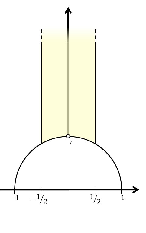
?figurename? 1: Fundamental domain $F_{2}$ for $\operatorname{SL}_{2}\left(\mathbb{Z}\right)$ in $P_{2}$ (the hyperbolic upper half plane).

Let us continue the analysis of the spaces $\mathcal{X}_{\underline{d}}$, $\mathcal{P}_{\underline{d}}$ and $\operatorname{Gr}(\underline{d},n)$ using the Refined Iwasawa decomposition. Our primary goal is to show how these spaces interact and to define measures on them. Let us begin with $\operatorname{Gr}(\underline{d},n)$. Recalling (3.1) and the fact that $\operatorname{Leb(\mathbb{S}^{i-1})}=i\cdot\mathfrak{V}(i)$ we have that

$$\|\mu_{K_{n}}\|=\prod_{i=1}^{n-1}\operatorname{Leb(\mathbb{S}^{i})}=\prod_{i=2}^{n}\operatorname{Leb(\mathbb{S}^{i-1})}=\frac{1}{2}\prod_{i=1}^{n}\operatorname{Leb(\mathbb{S}^{i-1})}=\frac{1}{2}\prod_{i=1}^{n}i\cdot\mathfrak{V}(i);$$ (4.1)

As $\operatorname{Gr}(\underline{d},n)\simeq K_{n}/\prod_{j=1}^{\ell}K_{d_{j}}$ (we use the notation $\simeq$ to indicate a diffeomorphism), we let $\mbox{vol}_{\operatorname{Gr}(\underline{d},n)}$ be the unique $K_{n}$-invariant measure on $\operatorname{Gr}(\underline{d},n)$ normalized such that

$$\|\mbox{vol}_{\operatorname{Gr}(\underline{d},n)}\| =\|\mu_{K_{n}}\|/\prod_{j=1}^{\ell}\|\mu_{K_{d_{j}}}\|.$$

By (4.1) this equals

$$=\frac{\frac{1}{2}\prod_{i=1}^{n}i\cdot\mathfrak{V}(i)}{\frac{1}{2^{\ell}}\prod_{i=1}^{\ell}\prod_{j=1}^{d_{i}}\prod_{i=1}^{n}j\cdot\mathfrak{V}(j)}=2^{\ell-1}\frac{n!}{d_{1}!\cdots d_{\ell}!}\frac{\prod_{i=1}^{n}\mathfrak{V}(i)}{\prod_{i=1}^{\ell}\prod_{j=1}^{d_{i}}\mathfrak{V}(j)}.$$

Naturally, we let $\mbox{vol}_{\operatorname{Gr}^{0}(\underline{d},n)}$ the $K_{n}$-invariant measure such that

$$\|\mbox{vol}_{\operatorname{Gr}^{0}(\underline{d},n)}\| =\frac{1}{2^{\ell-1}}\|\mbox{vol}_{\operatorname{Gr}(\underline{d},n)}\|=\frac{n!}{d_{1}!\cdots d_{\ell}!}\frac{\prod_{i=1}^{n}\mathfrak{V}(i)}{\prod_{i=1}^{\ell}\prod_{j=1}^{d_{i}}\mathfrak{V}(j)}.$$ (4.2)

On the remaining spaces, we define measures using the standard procedure of (i) presenting a space as a quotient of a homogeneous manifold by the action of a discrete group; (ii), identifying a fundamental domain in the manifold for that action; (iii) defining the measure on the space as the invariant measure on the manifold, restricted to the fundamental domain (or rather, the pullback of this measure through the inverse of the quotient map, which is one to one on the fundamental domain). Recall the following construction of fundamental domains representing

$$\begin{array}[]{ccccccccc}\mathcal{L}_{n}&=&\operatorname{SL}_{n}(\mathbb{R})/\operatorname{SL}_{n}(\mathbb{Z})&&\text{and}&&\mathcal{X}_{n}&=&\operatorname{SO}_{n}(\mathbb{R})\backslash\operatorname{SL}_{n}(\mathbb{R})/\operatorname{SL}_{n}(\mathbb{Z})\\ &&&&&&&\simeq&P_{n}/\operatorname{SL}_{n}(\mathbb{Z})\end{array}.$$

Let $F_{n}\subset P_{n}$ be the standard Siegel fundamental domain for right action of $\operatorname{SL}_{n}(\mathbb{Z})$ (see figure 1 for the case $n=2$). Let $\widetilde{F_{n}}$ be the lift of $F_{n}$ to $\operatorname{SL}_{n}(\mathbb{R})$, which is

$$\widetilde{F_{n}}=\bigcup_{z\in F_{n}}K_{z}\cdot z$$ (4.3)

([HK20b, Thm. 7.10 and Prop. 7.13]), where for every $z\in F_{n}$, the notation $K_{z}\subset\operatorname{SO}_{n}\left(\mathbb{R}\right)$ stands for a fundamental domain for the finite group of elements in $\operatorname{SO}(V_{\Lambda})$ that preserves $\Lambda$, $\mbox{Sym}^{+}(\Lambda_{z})$. It is known ([Sch98, Lem. 6]) that for almost every $z\in\operatorname{int}\left(F_{n}\right)$ one has that $\mbox{Sym}^{+}(\Lambda_{z})=Z(K)$ where $Z(K)$ is the center of $K$. Letting $K_{\text{gen}}$ denote the generic fiber, we have

$$\widetilde{F_{n}}=K_{\text{gen}}\cdot\operatorname{int}\left(F_{n}\right)\cup\bigcup_{z\in\partial F_{n}}K_{z}\cdot z$$ (4.4)

and therefore

$$\mu_{G_{n}}(\widetilde{F_{n}})=\mu_{K_{n}}(K_{n}/Z(K_{n}))\cdot\mu_{P^{\prime\prime}}(F_{n}),=\|\mu_{K_{n}}\|\mu_{P^{\prime\prime}}(F_{n})/\iota(n)$$

where

$$\iota(n)=[K_{n}:Z(K_{n})]=\begin{cases}1&n\equiv 1(\text{mod }2)\\ 2&n\equiv 0(\text{mod }2)\end{cases}.$$

We refer to [Gar14] for the fact that

$$\mu_{G_{n}}(\widetilde{F_{n}})=\prod_{i=2}^{n}\zeta\left(i\right).$$ (4.5)

Recalling (3.1) and the fact that $\operatorname{Leb(\mathbb{S}^{i-1})}=i\cdot\mathfrak{V}(i)$ we have that

$$\|\mu_{K_{n}}\|=\prod_{i=1}^{n-1}\operatorname{Leb(\mathbb{S}^{i})}=\prod_{i=2}^{n}\operatorname{Leb(\mathbb{S}^{i-1})}=\frac{1}{2}\prod_{i=1}^{n}\operatorname{Leb(\mathbb{S}^{i-1})}=\frac{1}{2}\prod_{i=1}^{n}i\cdot\mathfrak{V}(i);$$

then, by (4.4),

$$\mu_{P_{n}}(F_{n})=\mu_{G_{n}}(\widetilde{F_{n}})[K_{n}:Z(K_{n})]/\|\mu_{K_{n}}\|=2\iota(n)\frac{\prod_{i=2}^{d}\zeta\left(i\right)}{\prod_{i=1}^{n}i\cdot\mathfrak{V}(i)}\,.$$

The sets of representatives $F_{n}$, $\widetilde{F_{n}}$ and $K^{\prime}$ allow us to construct fundamental domains for $\mathcal{X}_{\underline{d}}$ and $\mathcal{P}_{\underline{d}}$. Quite naturally, a fundamental domain for $\mathcal{X}_{\underline{d}}\simeq P^{\prime\prime}/G^{\prime\prime}(\mathbb{Z})$ is

$$\prod_{j=1}^{\ell}F_{d_{j}}\subset P^{\prime\prime},\;\text{with}\;\,\mu_{P^{\prime\prime}}(\prod_{j=1}^{\ell}F_{d_{j}})=\prod_{j=1}^{\ell}\mu_{P_{d_{j}}}(F_{d_{j}}).$$

Also,

$$K^{\prime}\prod_{j=1}^{\ell}\widetilde{F_{d_{j}}}\subset K^{\prime}G^{\prime\prime}=Q$$

is a fundamental domain for

$$\mathcal{P}_{\underline{d}}=\operatorname{SL}_{n}\left(\mathbb{R}\right)/G^{\prime\prime}\left(\mathbb{Z}\right)N^{\prime}A^{\prime}=Q/G^{\prime\prime}\left(\mathbb{Z}\right),$$

and by (3.3) its measure in $Q$ is

$$\mu_{Q}(K^{\prime}\prod_{j=1}^{\ell}\widetilde{F_{d_{j}}})=\mu_{K^{\prime}}(K^{\prime})\mu_{G^{\prime\prime}}(\prod_{j=1}^{\ell}\widetilde{F_{d_{j}}}).$$

Now, the measures on $\mathcal{X}_{\underline{d}}$ and $\mathcal{P}_{\underline{d}}$ are defined so that they correspond to the homogeneous measures on the ambient manifolds, restricted to the fundemental domains. We list them for future reference:

Definition 4.1.

We let $\mbox{vol}_{\mathcal{L}_{n}}=\mu_{G_{n}}|_{\widetilde{F_{n}}}$ and $\mbox{vol}_{\mathcal{X}_{n}}=\mu_{P_{n}}|_{F_{n}}$ , so that

$$\|\mbox{vol}_{\mathcal{L}_{n}}\|=\prod_{i=2}^{n}\zeta\left(i\right),\quad\|\mbox{vol}_{\mathcal{X}_{n}}\|=2\iota(n)\frac{\prod_{i=2}^{d}\zeta\left(i\right)}{\prod_{i=1}^{n}i\cdot\mathfrak{V}(i)}.$$

Set $\mbox{vol}_{\mathcal{X}_{\underline{d}}}=\prod_{j=1}^{\ell}\mbox{vol}_{\mathcal{X}_{d_{j}}}$. Let $\mbox{vol}_{\mathcal{P}_{\underline{d}}}=\mu_{Q}|_{K^{\prime}\prod_{j=1}^{\ell}\widetilde{F_{d_{j}}}}$ so that in particular

$$\|\mbox{vol}_{\mathcal{P}_{\underline{d}}}\| =\|\mbox{vol}_{\operatorname{Gr}(\underline{d},n)}\|\cdot\prod_{j=1}^{\ell}\mbox{vol}_{\mathcal{L}_{d_{j}}}$$

$$=2^{\ell-1}\frac{n!}{d_{1}!\cdots d_{\ell}!}\frac{\prod_{i=1}^{n}\mathfrak{V}(i)}{\prod_{i=1}^{\ell}\prod_{j=1}^{d_{i}}\mathfrak{V}(j)}\cdot\prod_{j=1}^{\ell}\prod_{i=2}^{d_{j}}\zeta\left(i\right).$$

The probability measures corresponding to $\mbox{vol}_{\mathcal{P}_{\underline{d}}}$, $\mbox{vol}_{\mathcal{X}_{\underline{d}}}$, $\mbox{vol}_{\operatorname{Gr}(\underline{d},n)}$ (and appearing in Theorems 1.1 and 1.2) are denoted

$$\mbox{vol}_{\mathcal{P}_{\underline{d}}}^{1}\,,\,\mbox{vol}_{\mathcal{X}_{\underline{d}}}^{1}\,,\,\mbox{vol}_{\operatorname{Gr}(\underline{d},n)}^{1}.$$

The fundamental domains in Def. 4.1 represent the corresponding spaces not only in terms of the measure. They also have the property that the image of a “nice enough” set in the space, is a “nice enough” set in the associated fundamental domain. We denote by $Q_{\Xi}$ the image of $\Xi$ in $K^{\prime}\prod_{j=1}^{\ell}\widetilde{F_{d_{j}}}\subset Q$, by $P_{\mathcal{E}}^{\prime\prime}$ the image of $\mathcal{E}$ in $\prod F_{d_{j}}\subset P^{\prime\prime}$, by $K_{\Phi}^{\prime}$ the image of $\Phi\subseteq\operatorname{Gr}(\underline{d},n)$ in $K^{\prime}$, and so forth. To make precise what we mean by “nice enough”, consider the following definition.

Definition 4.2.

A subset $B$ of an orbifold $\mathcal{M}$ will be called boundary controllable if for every $x\in\mathcal{M}$ there is an open neighborhood $U_{x}$ of $x$ such that $U_{x}\cap\partial B$ is contained in a finite union of embedded $C^{1}$ submanifolds of $\mathcal{M}$, whose dimension is strictly smaller than $\dim\mathcal{M}$. In particular, $B$ is boundary controllable if its (topological) boundary consists of finitely many subsets of embedded $C^{1}$ submanifolds.

Lemma 4.3.

If a subset of any of the spaces appearing in Def. 4.1 is boundary controllable, then so is its image in the associated set of representatives (e.g. if $\Xi\subseteq\mathcal{P}_{\underline{d}}$ is boundary controllable, then so is $Q_{\Xi}$).

?proofname? .

If $\Xi\subseteq\mathcal{P}_{\underline{d}}$ is boundary controllable, then so is its lift to $Q$ (that is, its inverse image under the quotient map $Q\to Q/G^{\prime\prime}\left(\mathbb{Z}\right)=\mathcal{P}_{\underline{d}}$). The image $Q_{\Xi}$ is the intersection of this lift with the set of representatives $K^{\prime}\prod_{j=1}^{\ell}\widetilde{F_{d_{j}}}$, which is also boundary controllable. The intersection of two boundary controllable sets is boundary controllable. The other cases are handled similarly. ∎

Lemma 4.3 handles the connection between boundary controllable sets in the spaces $\mathcal{X}_{\underline{d}}$, $\mathcal{L}_{\underline{d}}$ and $\mathcal{P}_{\underline{d}}$ — namely spaces that are expressed as quotients by actions of discrete subgroups — to boundary controllable sets in the associated sets of representatives. But something similar can also be said for the space $\operatorname{Gr}(\underline{d},n)$, namely that $K^{\prime}$ can be chosen to satisfy the following property ([HK19, Lem. 3.4 (ii)]):

Condition 4.4.

The set of representatives $K^{\prime}\subset K$ satisfies that if $\Phi\subseteq\operatorname{Gr}(\underline{d},n)$ and $\mathcal{B}\subseteq K^{\prime\prime}$ are boundary controllable, then so is $K_{\Phi}^{\prime}\mathcal{B}\subseteq K$.

With the choice of volumes declared in Def. 4.1, we have the following relations between the spaces $\mathcal{P}_{\underline{d}}$, $\mathcal{X}_{\underline{d}}$ and $\operatorname{Gr}(\underline{d},n)$.

Proposition 4.5.

The following hold:

1. There exist natural projections from $\mathcal{P}_{\underline{d}}$ to $\mathcal{X}_{\underline{d}}$, to $\operatorname{Gr}(\underline{d},n)$, and to $\mathcal{X}_{\underline{d}}\times\operatorname{Gr}(\underline{d},n)$.

2. Assume that $\Xi\subseteq\mathcal{P}_{\underline{d}}$ is the inverse image of $\mathcal{E}\times\Phi\subseteq\mathcal{X}_{\underline{d}}\times\operatorname{Gr}(\underline{d},n)$ under the projection from part 1, $\pi_{\mathcal{P}_{\underline{d}}\to\mathcal{X}_{\underline{d}}\times\operatorname{Gr}(\underline{d},n)}$. If $\mathcal{E}\subseteq\mathcal{X}_{\underline{d}}$ and $\Phi\subseteq\operatorname{Gr}(\underline{d},n)$ are measurable, then so is $\Xi$ and

   $$\mbox{vol}_{\mathcal{P}_{\underline{d}}}(\Xi)=\mbox{vol}_{\mathcal{X}_{\underline{d}}}(\mathcal{E})\mbox{vol}_{\operatorname{Gr}(\underline{d},n)}(\Phi)\cdot\prod_{i=1}^{\ell}\iota(d_{i}).$$

3. If $\mathcal{E}$ and $\Phi$ are boundary controllable, then so is $\Xi$.

?proofname?.

For the first part: the projection $\pi_{\mathcal{P}_{\underline{d}}\to\mathcal{X}_{\underline{d}}}$ is given by quotienting from the left by $\operatorname{SO}_{n}(\mathbb{R})$, the projection $\pi_{\mathcal{P}_{\underline{d}}\to\operatorname{Gr}(\underline{d},n)}$ is the one induced by the projection $\operatorname{SL}_{n}(\mathbb{R})\to K/K^{\prime\prime}$ given by $kan\mapsto kK^{\prime\prime}$, and the projection $\pi_{\mathcal{P}_{\underline{d}}\to\mathcal{X}_{\underline{d}}\times\operatorname{Gr}(\underline{d},n)}$ is the product of the latter two. For the second and third parts, let $\widetilde{\mathcal{E}}\subseteq\mathcal{L}_{\underline{d}}$ be the inverse image of $\mathcal{E}$ under the natural projection $\mathcal{L}_{\underline{d}}\to\mathcal{X}_{\underline{d}}$. By (4.4),

$$Q_{\Xi}=K_{\Phi}^{\prime}G_{\widetilde{\mathcal{E}}}^{\prime\prime}=\left(K_{\Phi}^{\prime}K_{\text{gen}}^{\prime\prime}\cdot(P_{\mathcal{E}}^{\prime\prime}\cap\prod_{j=1}^{\ell}\operatorname{int}\left(F_{d_{j}}\right))\right)\cup\bigcup_{z\in P_{\mathcal{E}}^{\prime\prime}\cap\partial\prod_{j=1}^{\ell}F_{d_{j}}}K_{\Phi}^{\prime}K_{z}^{\prime\prime}\cdot z.$$

It is sufficient to show that the image of $Q_{\Xi}$ under the diffeomorphism $Q\to K\times P^{\prime\prime}$, which is obvious from the above equation, is boundary controllable. As for the $K$ part of this image, we have that every $K_{z}^{\prime\prime}$ (and in particular $K_{\text{gen}}^{\prime\prime}$) is boundary controllable in $K^{\prime\prime}$, and hence by Condition 4.4 every $K_{\Phi}^{\prime}K_{z}^{\prime\prime}$ is boundary controllable in $K$. As for the $P^{\prime\prime}$ part of this image, we have that: $P_{\mathcal{E}}^{\prime\prime}$ is boundary controllable, because of the assumption on $\mathcal{E}$ and Lemma 4.3; $\operatorname{int}\left(F_{n}\right)$ is boundary controllable, since $F_{n}$ is; hence $P_{\mathcal{E}}^{\prime\prime}\cap\operatorname{int}\left(F_{n}\right)$ is boundary controllable, as an intersection of such. Moreover $P_{\mathcal{E}}^{\prime\prime}\cap\partial F_{n}$ is boundary controllable, since it is its own boundary. We conclude that $Q_{\Xi}$ is boundary controllable, and therefore $\Xi$ is. This proves the third part, but also that

$$\mu_{Q}(Q_{\Xi})=\mu_{K^{\prime}}(K_{\Phi}^{\prime})\mu_{K^{\prime\prime}}(K_{\text{gen}}^{\prime\prime})\mu_{P^{\prime\prime}}(P_{\mathcal{E}}^{\prime\prime})=\mu_{K^{\prime}}(K_{\Phi}^{\prime})\mu_{P^{\prime\prime}}(P_{\mathcal{E}}^{\prime\prime})/[K^{\prime\prime}:Z(K^{\prime\prime})],$$

where in the first equality we used $\mu_{Q}=\mu_{K^{\prime}}\times\mu_{G^{\prime\prime}}$ and $\mu_{G^{\prime\prime}}=\mu_{K^{\prime\prime}}\times\mu_{P^{\prime\prime}}$ ((3.6)). Since $[K^{\prime\prime}:Z(K^{\prime\prime})]=\prod_{i=1}^{\ell}\iota(d_{i})$, and by Def. 4.1, we confirm the third statement. ∎

5 A more general theorem

The natural map from the space $\mathcal{P}_{\underline{d}}$ to $\mathcal{X}_{\underline{d}}\times\operatorname{Gr}(\underline{d},n)$ (Prop. 4.5) hints at the fact that counting primitive integral flags w.r.t their projections to $\mathcal{P}_{\underline{d}}$ would imply counting these flags w.r.t. their projections to $\mathcal{X}_{\underline{d}}\times\operatorname{Gr}(\underline{d},n)$, which is the content of Theorems 1.1 and 1.2. Indeed, in this section we state a counting theorem with $\mathcal{P}_{\underline{d}}$, from which we deduce Theorems 1.1 and 1.2. Recall from Section 2 that the projection of a flag of lattices $\mathbf{F}(\mathbb{Z})$ to the space $\mathcal{P}_{\underline{d}}$ is denoted by $\left[\mathbf{F}(\mathbb{Z})\right]$. In what follows, we say that $\Xi\subseteq\mathcal{P}_{\underline{d}}$ is bounded if $\pi_{\mathcal{P}_{\underline{d}}\to\mathcal{X}_{\underline{d}}}(\Xi)$ is.

Theorem 5.1.

Let $\tau_{n}=(4n^{2}/\left\lceil\left(n-1\right)/2\right\rceil)^{-1}$, and assume that $\Xi\subseteq\mathcal{P}_{\underline{d}}$ is boundary controllable. The number of positive primitive integral $\underline{d}$-flags $\mathbf{F}(\mathbb{Z})$ with $\left[\mathbf{F}(\mathbb{Z})\right]\in\Xi$ and $H(\mathbf{F}(\mathbb{Z}))\leq e^{T}$ is

$$2^{\ell-1}c_{\underline{d},n}\cdot\mbox{vol}_{\mathcal{P}_{\underline{d}}}^{\,1}(\Xi)\cdot e^{hT}+\text{error term}$$

where

$$h=\begin{cases}2n-d_{1}-d_{\ell}&\text{if $H=H_{\infty}$}\\ 1&\text{if $H=H_{\operatorname{ac}}$}\end{cases}$$ (5.1)

and the error term is $O_{\epsilon}(e^{hT(1-\frac{\tau_{n}n}{\beta}+\epsilon)})$ for every $\epsilon>0$, where

$$\beta=\begin{cases}1&\text{if $\Xi$ is bounded}\\ 2\left(n-\ell\right)\left(n^{2}-1\right)+n^{2}&\text{if $\Xi$ is not bounded}\end{cases}.$$

Proof of Theorems 1.1 and 1.2 assuming Theorem 5.1..

Let $\mathcal{E}\subseteq\mathcal{X}_{\underline{d}}$ and $\Phi\subseteq\operatorname{Gr}^{0}(\underline{d},n)$ be boundary controllable. We denote by $\tilde{\Phi}\subseteq\operatorname{Gr}(\underline{d},n)$ the lift of $\Phi$ to $\operatorname{Gr}(\underline{d},n)$, which is also boundary controllable. By Proposition 4.5 the set

$$\Xi=\pi_{\mathcal{P}_{\underline{d}}\to\mathcal{X}_{\underline{d}}\times\operatorname{Gr}(\underline{d},n)}^{-1}(\mathcal{E}\times\tilde{\Phi})$$

is boundary controllable and $\mbox{vol}_{\mathcal{P}_{\underline{d}}}(\Xi)=\mbox{vol}_{\mathcal{X}_{\underline{d}}}(\mathcal{E})\mbox{vol}_{\operatorname{Gr}(\underline{d},n)}(\tilde{\Phi})\prod_{i=1}^{\ell}\iota(d_{i})$. In particular, for $\mathcal{E}=\mathcal{X}_{\underline{d}}$ and $\tilde{\Phi}=\operatorname{Gr}(\underline{d},n)$ we have that

$$\|\mbox{vol}_{\mathcal{P}_{\underline{d}}}\|=\|\mbox{vol}_{\mathcal{X}_{\underline{d}}}\|\|\mbox{vol}_{\operatorname{Gr}(\underline{d},n)}\|\prod_{i=1}^{\ell}\iota(d_{i}).$$

Then, by Theorem 5.1, the number of positive primitive integral $\underline{d}$-flags $\mathbf{F}(\mathbb{Z})$ with $\left[\mathbf{F}(\mathbb{Z})\right]\in\Xi$ and $H(\mathbf{F}(\mathbb{Z}))\leq e^{T}$ is

$$\approx 2^{\ell-1}c_{\underline{d},n}\cdot\frac{\mbox{vol}_{\mathcal{P}_{\underline{d}}}(\Xi)}{\|\mbox{vol}_{\mathcal{P}_{\underline{d}}}\|}\cdot e^{hT}=2^{\ell-1}c_{\underline{d},n}\cdot\frac{\mbox{vol}_{\mathcal{X}_{\underline{d}}}(\mathcal{E})\,\mbox{vol}_{\operatorname{Gr}(\underline{d},n)}(\tilde{\Phi})}{\|\mbox{vol}_{\mathcal{X}_{\underline{d}}}\|\|\mbox{vol}_{\operatorname{Gr}(\underline{d},n)}\|}\cdot e^{hT}$$

$$=2^{\ell-1}c_{\underline{d},n}\cdot\mbox{vol}_{\mathcal{X}_{\underline{d}}}^{1}(\mathcal{E})\mbox{vol}_{\operatorname{Gr}(\underline{d},n)}^{1}(\tilde{\Phi})\cdot e^{hT}=c_{\underline{d},n}\cdot\mbox{vol}_{\mathcal{X}_{\underline{d}}}^{1}(\mathcal{E})\mbox{vol}_{\operatorname{Gr}^{0}(\underline{d},n)}^{1}(\Phi)\cdot e^{hT},$$

where in the last equality we used (4.2). ∎

The rest of this article is devoted to proving Theorem 5.1.

6 Integral matrices correspond to integral flags

The goal of this section is to translate the statement of Theorem 5.1 into a counting problem of integral matrices. To do so, we establish a correspondence between integral unimodular $\underline{d}$-flags and integral matrices in a fundamental domain of the following discrete group of $\operatorname{SL}_{n}(\mathbb{R})$:

$$\Gamma^{\prime}=\left(N^{\prime}\rtimes G^{\prime\prime}\right)\left(\mathbb{Z}\right)=\left[\begin{smallmatrix}\operatorname{SL}_{d_{1}}\left(\mathbb{Z}\right)&\mathbb{Z}^{d_{1}\times d_{2}}&\cdots&\mathbb{Z}^{d_{1}\times d_{\ell}}\\ 0&\ddots&\ddots&\vdots\\ \vdots&\ddots&\operatorname{SL}_{d_{\ell-1}}\left(\mathbb{Z}\right)&\mathbb{Z}^{d_{\ell-1}\times d_{\ell}}\\ 0&\cdots&0&\operatorname{SL}_{d_{\ell}}\left(\mathbb{Z}\right)\end{smallmatrix}\right].$$

Proposition 6.1.

There exists a bijection $\mathbf{F}\leftrightarrow\gamma_{\mathbf{F}}$ between integral unimodular $\underline{d}$-flags and integral matrices in a fundamental domain of $\operatorname{SL}_{n}\left(\mathbb{R}\right)\curvearrowleft\Gamma^{\prime}$, that sends a unimodular $\underline{d}$-flag $\mathbf{F}$ to $\gamma_{\mathbf{F}}$, the unique integral matrix in the fundamental domain whose columns span $\mathbf{F}$.

?proofname?.

The direction $\Leftarrow$ is simple: given $\gamma\in\Omega\cap\operatorname{SL}_{n}\left(\mathbb{Z}\right)$, its columns span $\mathbb{Z}^{n}$ hence by definition a $\underline{d}$ partition of its columns spans a unimodular integral $\underline{d}$–flag. In the opposite direction, let $\mathbf{B}_{1}|\cdots|\mathbf{B}_{\ell}$ be a basis for $\mathbf{F}$. Since $\mathbf{F}$ is primitive, we may assume that $\mathbf{B}_{\ell}$ is also a basis for $\mathbb{Z}^{n}$; let $\gamma\in\operatorname{SL}_{n}\left(\mathbb{Z}\right)$ be a matrix having this basis in its columns. The orbit $\gamma\cdot\Gamma$ meets $\Omega$ in a single point, $\gamma_{\mathbf{F}}$. ∎

Let us construct an explicit fundamental domain for $\Gamma^{\prime}$. Denote

$$\square=\text{the unit cube $\left(-1/2,1/2\right]^{\dim(N^{\prime})}$},$$

let $N^{\prime}_{\square}$ be the image of $\square$ in $N^{\prime}$, and set

$$\Omega=K^{\prime}G^{\prime\prime}_{\widetilde{F_{d_{1}}}\times\cdots\times\widetilde{F_{d_{\ell}}}}A^{\prime}N^{\prime}_{\square}\,.$$

It is easy to see that $\Omega$ is a fundamental domain for the right action of $\Gamma^{\prime}$ on $\operatorname{SL}_{n}\left(\mathbb{R}\right)$.

Proposition 6.1 confirms that every unimodular integral flag is represented by a unique integral matrix in $\Omega$; the next step is to verify how the different properties of the flag — e.g. its shape, or the covolumes of the lattices that compose it — are exhibited in the Refined Iwasawa components of the matrix that spans the flag.

For $g\in\operatorname{GL}_{n}(\mathbb{R})$, recall the notation for the primitive $\underline{d}$-flag of lattices spanned by the columns of $g$:

$$\mathbf{F}_{g}(\mathbb{Z})=\>(\,\Lambda_{g}^{(1)}<\Lambda_{g}^{(2)}<\cdots<\Lambda_{g}^{(\ell)}=\Lambda_{g}<\mathbb{R}^{n}\,).$$

By setting

$$D_{j}=\sum_{i=1}^{j}d_{i},$$

we have that each $\Lambda_{g}^{(j)}$ is the $\mathbb{Z}$-span of the first $D_{j}$ columns of $g$. For $D_{j-1}+1\leq i\leq D_{j}$, we let

$$(\Lambda_{g}^{(j)})^{i}$$

be the subgroup of $\Lambda_{g}^{(j)}$ spanned by the columns $[D_{j-1}+1,i]$ of $g$. The consecutive quotients are

$$L_{j}(g)=\Lambda_{g}^{(j)}/\Lambda_{g}^{(j-1)},$$

that is, each $L_{j}(g)$ is spanned by the cosets of $\Lambda_{g}^{(j-1)}$ that are generated by the columns $[D_{j-1}+1,D_{j}]$ of $g$. Let

$$L_{j}(g)^{i}$$

be the subgroup of $L_{j}(g)$ spanned by the cosets corresponding to columns $[D_{j-1}+1,i]$.

Proposition 6.2.

Assume $g\in\operatorname{SL}_{n}\left(\mathbb{R}\right)$ is written in Refined Iwasawa coordinates as

$$g=kan=qa^{\prime}n^{\prime}$$

where

$$a^{\prime} =a_{t_{1},\ldots,t_{\ell-1}}^{\prime}$$

$$q =k^{\prime}g^{\prime\prime}=k^{\prime}k^{\prime\prime}p^{\prime\prime}a_{\underline{s}^{(1)},\ldots,\underline{s}^{(\ell)}}^{\prime\prime}n^{\prime\prime}.$$

for every $j=1,\ldots,\ell$, let $g^{\prime\prime}=\operatorname{diag}(g_{d_{1}},\ldots,g_{d_{\ell}})$, $g_{d_{j}}^{\prime\prime}=\operatorname{diag}(I_{d_{1}},\ldots,g_{d_{j}},\ldots,\operatorname{I}_{d_{\ell}})$, and similarly for $p^{\prime\prime}$. The Refined Iwasawa components of $g$ represent parameters related to $\mathbf{F}_{g}(\mathbb{Z})$ in the following way:

$$\begin{array}[]{ccccc}(i)&\mathbf{F}_{k^{\prime}}&=&\mathbf{F}_{g}\\ (ii)&e^{t_{j}}&=&\operatorname{covol}(\Lambda_{g}^{(j)})\\ (ii)^{\prime}&e^{t_{j}-t_{j-1}}&=&\operatorname{covol}(L_{j}(g))&(t_{0}=t_{\ell}=0)\\ (iii)&e^{\frac{i(t_{j}-t_{j-1})}{d_{j}}-\frac{s_{i}^{(j)}}{2}}&=&\operatorname{covol}(L_{j}(g)^{i})\\ (iii)^{\prime}&e^{\frac{\hat{i}t_{j}+(d_{j}-\hat{i})t_{j-1}}{d_{j}}-\frac{s_{\hat{i}}^{(j)}}{2}}&=&\operatorname{covol}(\Lambda^{(j)}{}^{i})&\left(\begin{subarray}{c}D_{j-1}+1\leq i\leq D_{j}\\ \hat{i}=i-d_{j-1}\end{subarray}\right)\\ (iv)&\left[\mathbf{F}_{q}(\mathbb{Z})\right]&=&\left[\mathbf{F}_{g}(\mathbb{Z})\right]\\ (v)&\operatorname{shape}\left(L_{j}\right)&=&\operatorname{shape}\left(\Lambda_{p_{d_{j}}}\right)\end{array}$$

?proofname?.

Since the columns of $k$ are obtained by performing the Gram-Schmidt orthogonalization procedure on the columns of $g$, we have for every $1\leq d\leq n$ that the first $d$ columns of $k$ span the same space as the first $d$ columns of $g$. Hence $\mathbf{F}_{g}=\mathbf{F}_{k}$. Since $k^{\prime}=k\left(k^{\prime\prime}\right)^{-1}$, where $k^{\prime\prime}\in G^{\prime\prime}$ fixes $\mathbf{F}_{g}$, we deduce that $(i)$ indeed holds.

Now write $g(n^{\prime})^{-1}(a^{\prime})^{-1}=q$; by definition, right multiplication by an element of $N^{\prime}A^{\prime}$ does not change the projection to $\mathcal{P}_{\underline{d}}$. This observation immediately proves part $(iv)$. As the shape of each $g_{d_{j}}^{\prime\prime}$ is the same as that of $p_{d_{j}}^{\prime\prime}$, part $(v)$ follows from part $(iv)$.

Notice that since $g^{\prime\prime}$ is in $G^{\prime\prime}$, the lattice flag $\mathbf{F}_{g^{\prime\prime}}(\mathbb{Z})$ is unimodular. Furthermore, as $q$ is a rotation of $g^{\prime\prime}$, the same holds for $\mathbf{F}_{q}(\mathbb{Z})$. As a result, using the fact that right multiplication by $n^{\prime}$ does not change the flag $\mathbf{F}_{q}(\mathbb{Z})$, we have

$$\operatorname{covol}(L_{j}^{i}(g))=\operatorname{covol}(L_{j}^{i}(qa^{\prime}))=\operatorname{covol}(L_{j}^{i}(a^{\prime}))=\operatorname{covol}((a^{\prime})^{D_{j}+i})=e^{\frac{i\left(t_{j}-t_{j-1}\right)}{d_{j}}-\frac{s_{i}^{(j)}}{2}}.$$

This proves parts $(iii)$ and $(ii)^{\prime}$.

Notice that if $\Lambda_{1}<\Lambda_{2}$ are lattices, then

$$\operatorname{covol}(\Lambda_{2})=\operatorname{covol}(\Lambda_{1})\operatorname{covol}(\Lambda_{2}/\Lambda_{1}).$$

As a result, parts $(ii)$ and $(iii)^{\prime}$ follow from parts $(iii)$ and $(ii)^{\prime}$. ∎

Remark 6.3.

Proposition 6.2 above explicates the projections from $\mathcal{P}_{\underline{d}}$ to $\mathcal{X}_{\underline{d}}$ and to $\operatorname{Gr}(\underline{d},n)$ that appear in Proposition 4.5: the projection of $\mathbf{F}_{g}(\mathbb{Z})$ to $\mathcal{P}_{\underline{d}}$ is $q=k^{\prime}k^{\prime\prime}p^{\prime\prime}$, while $p^{\prime\prime}$ represents the projection to $\mathcal{X}_{\underline{d}}$, and $k^{\prime}$ represents the projection to $\operatorname{Gr}(\underline{d},n)$.

We can now define subsets of $\Omega$ that capture only the integral matrices corresponding to unimodular lattice flags with certain shape, direction, and height. For $T>0$ denote:

$$A^{\prime}_{T} :=\{a_{t_{1},\ldots,t_{\ell-1}}^{\prime}:\log\left(H_{\infty}(t_{1},\ldots,t_{\ell-1})\right)\leq T\}$$

$$=\{a_{t_{1},\ldots,t_{\ell-1}}^{\prime}:0\leq t_{i}\leq T\;\forall i=1,\ldots,\ell-1$$

and

$${}_{T}A^{\prime} :=\{a_{t_{1},\ldots,t_{\ell-1}}^{\prime}:\log\left(H_{\operatorname{ac}}(t_{1},\ldots,t_{\ell-1})\right)\leq T\}$$

$$=\{a_{t_{1},\ldots,t_{\ell-1}}^{\prime}:\sum_{i=1}^{\ell-1}t_{i}(d_{i}+d_{i+1})\leq T\}.$$

Also, let

$${}_{T}A^{\prime}_{T}=\begin{cases}A^{\prime}_{T}&\text{if $H=H_{\infty}$}\\ {}_{T}A^{\prime}&\text{if $H=H_{\operatorname{ac}}$}\end{cases}.$$

Notation 6.4.

For $T>0$ and $\Xi\subseteq\mathcal{P}_{\underline{d},n}$, consider

$$\Omega_{T}(\Xi)=\,\Omega\,\cap\,\left\{g=qa^{\prime}n^{\prime}:q\in Q_{\Xi},a^{\prime}\in A^{\prime}_{T}\right\}=Q_{\Xi}A^{\prime}_{T}N^{\prime}_{\square}.$$

Similarly, denote

$${}_{T}\Omega(\Xi)=\,\Omega\,\cap\,\left\{g=qa^{\prime}n^{\prime}:q\in Q_{\Xi},a^{\prime}\in_{T}A^{\prime}\right\}=Q_{\Xi}\>{}_{T}A^{\prime}N^{\prime}_{\square}$$

for the analogous set where $A^{\prime}_{T}$ is replaced by ${}_{T}A^{\prime}$. Finally,

$${}_{T}\Omega_{T}(\Xi)=Q_{\Xi}\>{}_{T}A^{\prime}_{T}N^{\prime}_{\square}=\begin{cases}\Omega_{T}(\Xi)&\text{if $H=H_{\infty}$}\\ {}_{T}\Omega(\Xi)&\text{if $H=H_{\operatorname{ac}}$}\end{cases}.$$

The following is immediate from Propositions 6.1 and 6.2:

Corollary 6.5.

Consider the correspondence $\mathbf{F}\leftrightarrow\gamma_{\mathbf{F}}$ between integral umimodular $\underline{d}$–flags and matrices in $\Omega\cap\operatorname{SL}_{n}\left(\mathbb{Z}\right)$, and let $T>0$. Then

$$\Omega_{T}(\Xi)\cap\operatorname{SL}_{n}\left(\mathbb{Z}\right) = \left\{\gamma_{\mathbf{F}}:H_{\infty}(\mathbf{F})\leq e^{T},\left[\mathbf{F}(\mathbb{Z})\right]\in\Xi\right\},$$

$${}_{T}\Omega(\Xi)\cap\operatorname{SL}_{n}\left(\mathbb{Z}\right) = \left\{\gamma_{\mathbf{F}}:H_{\operatorname{ac}}(\mathbf{F})\leq e^{T},\left[\mathbf{F}(\mathbb{Z})\right]\in\Xi\right\}.$$

7 Some volume computations

The goal of this section is to compute the volumes of the sets $\Omega_{T}(\Xi)$ and ${}_{T}\Omega(\Xi)$, introduced in Notation 6.4. From now on, we will abbreviate and let $\mu=\mu_{G_{n}}$.

Proposition 7.1.

$$\mu(\Omega_{T}(\Xi))=\frac{\mbox{vol}_{\mathcal{P}_{\underline{d}}}(\Xi)}{\prod_{j=1}^{\ell-1}(d_{j}+d_{j+1})}\cdot e^{T(2n-d_{1}-d_{\ell})}+O(e^{T\left(2n-d_{1}-d_{\ell}-2\right)}).$$

and

$$\mu(_{T}\Omega(\Xi))=\frac{\mbox{vol}_{\mathcal{P}_{\underline{d}}}(\Xi)}{\prod_{j=1}^{\ell-1}(d_{j}+d_{j+1})}\cdot e^{T}\sum_{i=0}^{\ell-2}(-1)^{\ell-2-i}\cdot\frac{T^{i}}{i!}+O(1).$$

For the proof, consider the following computational lemma.

Lemma 7.2.

Let

$$f_{m}(T)=\int_{0}^{T}e^{x_{m}}\int_{0}^{T-x_{m}}e^{x_{m-1}}\cdots\int_{0}^{T-x_{2}-\cdots-x_{m}}e^{x_{1}}dx_{1}\cdots dx_{m}.$$

Then

$$f_{m}(T)=e^{T}\cdot\sum_{i=0}^{m-1}(-1)^{m-i-1}\frac{T^{i}}{i!}+(-1)^{m}.$$

?proofname?.

Notice that for $m>1$

$$f_{m}(T)=\int_{0}^{T}f_{m-1}(T-s_{m})e^{s_{m}}ds_{m},$$

and so we will prove the claim by induction on $m$. When $m=1$ we have that:

$$f_{1}(T)=\int_{0}^{T}e^{x_{1}}dx_{1}=e^{T}-1=e^{T}\sum_{i=0}^{0}(-1)^{-i}\frac{T^{i}}{i!}+(-1)^{1}.$$

Assume that the claim holds for some $m-1\geq 1$. We have:

$$f_{m}(T) =\int_{0}^{T}f_{m-1}(x_{m}-T)e^{x_{m}}dx_{m}$$

$$=\int_{0}^{T}\left(e^{T}\cdot\sum_{i=0}^{m-2}(-1)^{m-i-2}\frac{(T-x_{m})^{i}}{i!}+(-1)^{m-1}e^{x_{m}}\right)dx_{m}$$

$$=e^{T}\cdot\sum_{i=0}^{m-2}(-1)^{m-i-1}\frac{(T-x_{m})^{i+1}}{(i+1)!}+(-1)^{m-1}e^{x_{m}}|_{x_{m}=0}^{x_{m}=T}$$

$$=e^{T}\cdot\sum_{i=0}^{m-2}(-1)^{m-(i+1)-1}\frac{T^{i+1}}{(i+1)!}+(-1)^{m-1}e^{T}+(-1)^{m}.$$

Set $j=i+1$ and then

$$=e^{T}\cdot\sum_{j=1}^{m-1}(-1)^{m-j-1}\frac{T^{j}}{j!}+(-1)^{m-1}e^{T}+(-1)^{m}$$

$$=e^{T}\cdot\sum_{j=0}^{m-1}(-1)^{m-j-1}\frac{T^{j}}{j!}+(-1)^{m}.\qed$$

Proof of Proposition 7.1.

By definition, ${}_{T}\Omega_{T}(\Xi)=Q_{\Xi}\>{}_{T}A^{\prime}_{T}N^{\prime}_{\square}$. From (3.6),

$$\mu(_{T}\Omega_{T}(\Xi)) = \mu_{Q}(Q_{\Xi})\mu_{A^{\prime}}(_{T}A^{\prime}_{T})\mu_{N^{\prime}}(N^{\prime}_{\square}),$$

where by Proposition 4.1 and the definition of $\mu_{N^{\prime}}$,

$$\mu_{Q}(Q_{\Xi}) = \mbox{vol}_{\mathcal{P}_{\underline{d}}}(\Xi)$$

$$\mu_{N^{\prime}}(N^{\prime}_{\square}) = \operatorname{Leb(\square)}=1\,.$$

It is therefore left to compute the $\mu_{A^{\prime}}$-volumes of $A^{\prime}_{T}$ and ${}_{T}A^{\prime}$. Referring to (3.2),

$$\mu_{A^{\prime}}(A^{\prime}_{T}) =\prod_{j=1}^{\ell-1}\int_{0}^{T}e^{\left(d_{j}+d_{j+1}\right)t_{j}}dt_{j}=\prod_{j=1}^{\ell-1}\frac{e^{\left(d_{j}+d_{j+1}\right)T}-1}{d_{j}+d_{j+1}}$$

$$=\frac{e^{T\cdot\sum_{j=1}^{\ell-1}\left(d_{j}+d_{j+1}\right)}}{\prod_{j=1}^{\ell-1}(d_{j}+d_{j+1})}+O(e^{T\cdot(\sum_{j=1}^{\ell-1}\left(d_{j}+d_{j+1}\right)-\min_{j}\{d_{j}+d_{j+1}\})}).$$

Note that

$$\sum_{j=1}^{\ell-1}\left(d_{j}+d_{j+1}\right)=\sum_{j=1}^{\ell-1}d_{j}+\sum_{j=2}^{\ell}d_{j}=(n-d_{\ell})+(n-d_{1})$$

(since $d_{1}+\cdots+d_{\ell}=n$). Therefore

$$\mu_{A^{\prime}}(A_{T}^{\prime})=\prod_{j=1}^{\ell-1}\frac{1}{d_{j}+d_{j+1}}e^{T\cdot\left(2n-d_{1}-d_{\ell}\right)}+O(e^{T\cdot\left(2n-d_{1}-d_{\ell}-2\right)}).$$

Moving on to ${}_{T}A^{\prime}$ and applying Lemma 7.2,

$$\mu_{A^{\prime}}(_{T}A^{\prime}) =\frac{f_{\ell-1}(T)}{\prod_{j=1}^{\ell-1}(d_{j}+d_{j+1})}f_{\ell-1}(T)=$$

$$=\frac{e^{T}}{\prod_{j=1}^{\ell-1}(d_{j}+d_{j+1})}\cdot\sum_{i=0}^{\ell-2}(-1)^{\ell-2-i}\frac{T^{i}}{i!}+O(1).\qed$$

8 Counting lattice points

As Corollary 6.5 suggests, Theorem 5.1 is proved by counting $\operatorname{SL}_{n}\left(\mathbb{Z}\right)$ matrices inside the sets $\Omega_{T}(\Xi)$ and ${}_{T}\Omega(\Xi)$. More precisely, this theorem follows from a counting lattice points statement of the form

$$\#(_{T}\Omega_{T}(\Xi)\cap\operatorname{SL}_{n}\left(\mathbb{Z}\right))=\mu(\operatorname{SL}_{n}(\mathbb{R})/\operatorname{SL}_{n}(\mathbb{Z}))^{-1}\cdot\mu(_{T}\Omega_{T}(\Xi))+O(\mu(_{T}\Omega_{T}(\Xi)))^{\kappa}$$

for some $0<\kappa<1$. However, the sets ${}_{T}\Omega_{T}(\Xi)$ are not compact when $\Xi$ is not compact (which is equivalent to the fact that the projection of $\Xi$ to $\mathcal{X}_{\underline{d}}$ is not compact), even though they have finite volume and contain a finite amount of lattice points. The way to address this problem is by splitting each set ${}_{T}\Omega_{T}(\Xi)$ into a compact subset and an “infinite tail”. In the present section we define a family of compact subsets of ${}_{T}\Omega_{T}(\Xi)$, and apply a known ergodic method [GN12] to count lattice points in this family. In Section 9, we apply direct counting to bound the amount of points in the “infinite tail”.

The family of compact subsets of ${}_{T}\Omega_{T}(\Xi)$ that we consider in this section is defined as follows. For

$$\underline{S}=(S_{1}^{(1)},\ldots,S_{d_{1}-1}^{(1)},\dots,S_{1}^{(\ell)},\ldots,S_{d_{\ell}-1}^{(\ell)})>\underline{0}$$ (8.1)

and a subset $\mathcal{B}\subset\operatorname{SL}_{n}(\mathbb{R})$, let $\mathcal{B}^{\underline{S}}$ denote the set

$$\mathcal{B}^{\underline{S}}=\mathcal{B}\cap\{g=ka^{\prime}a_{\underline{s}}^{\prime\prime}n:s^{(j)}_{i}\leq S_{i}^{(j)}\;\,\forall 1\leq i<d_{j},1\leq j\leq\ell\}.$$

Specifically, let

$${}_{T}\Omega_{T}^{\underline{S}} =K^{\prime}G^{\prime\prime}_{\widetilde{F_{d_{1}}}^{\underline{S}^{(1)}}\times\cdots\times\widetilde{F_{d_{\ell}}}^{\underline{S}^{(\ell)}}}\,{}_{T}A^{\prime}_{T}N^{\prime}_{\square}.$$

One can deduce from the proof of Proposition 7.1 that

$$\mu(_{T}\Omega_{T}-_{T}\Omega_{T}^{\underline{S}})=O(e^{hT-S_{\min}})$$ (8.2)

where $S_{\min}=\min_{i,j}S_{i}^{(j)}$ and $h$ was defined in (5.1). Indeed,

$$\mu\left({}_{T}\Omega_{T}-_{T}\Omega_{T}^{\underline{S}}\right) =O\left(\mu_{A}(_{T}A^{\prime}_{T}A^{\prime\prime}-_{T}A^{\prime}_{T}(A^{\prime\prime})^{\underline{S}})\right)$$

where $\mu_{A}(_{T}A^{\prime}_{T}A^{\prime\prime}-_{T}A^{\prime}_{T}(A^{\prime\prime})^{\underline{S}})$ equals $\mu_{A^{\prime}}(_{T}A^{\prime}_{T})\mu_{A^{\prime\prime}}(A^{\prime\prime}-(A^{\prime\prime})^{\underline{S}})$, as $\mu_{A}=\mu_{A^{\prime}}\times\mu_{A^{\prime\prime}}$. In the proof of Prop. 7.1 it was shown that $\mu_{A^{\prime}}(_{T}A^{\prime}_{T})\ll e^{hT}$; now

$$\mu_{A^{\prime\prime}}\left(A^{\prime\prime}-(A^{\prime\prime})^{\underline{S}}\right) =\int_{\left[0,\infty\right)^{n-\ell}-\prod_{j=1}^{n-\ell}\left[0,S_{j}\right]}d\mu_{A^{\prime\prime}}$$

$$\ll e^{(2n-d_{1}-d_{\ell})T}\cdot\sum_{j=1}^{n-\ell}\int_{\left(S_{j}\leq s_{j}<\infty\right)\times\prod_{i\neq j}\left(0\leq s_{i}<\infty\right)}\frac{du_{1}\cdots du_{n-\ell}}{e^{u_{1}+\cdots+u_{n-\ell}}}$$

$$\ll e^{(2n-d_{1}-d_{\ell})T}\cdot\left(e^{-s_{1}}+\cdots+e^{-s_{n-\ell}}\right)$$

$$\ll e^{(2n-d_{1}-d_{\ell})T}\cdot e^{-\min S_{i}}.$$

In order to count $\operatorname{SL}_{n}(\mathbb{Z})$ elements in $\Omega_{T}^{\underline{S}}$ and ${}_{T}\Omega^{\underline{S}}$, we will employ a method that was developed by Gorodnik and Nevo in [GN12]. This method produces counting statements for lattice subgroups of Lie groups, including an error estimate. The bound on the error exponent involves a parameter $\tau$ that we now turn to define.

Let $\Gamma$ be a lattice subgroup of a simple algebraic Lie group $G$, that is, $\Gamma$ is discrete and $\operatorname{Haar}_{G}(G/\Gamma)<\infty.$ There exists $p\in\mathbb{N}$ for which the matrix coefficients $\langle\pi_{G/\Gamma}^{0}u,v\rangle$ are in $L^{p+\epsilon}\left(G\right)$ for every $\epsilon>0$, with $u,v$ lying in a dense subspace of $L_{0}^{2}\left(G/\Gamma\right)$ (see [GN09, Thm. 5.6]). Let $p\left(\Gamma\right)$ be the smallest among these $p$’s, and denote

$$m\left(\Gamma\right)=\begin{cases}1&\text{if $p=2$,}\\ 2\left\lceil p\left(\Gamma\right)/4\right\rceil&\text{otherwise}\end{cases},$$

$$\tau\left(\Gamma\right)=\frac{1}{2m\left(\Gamma\right)\left(1+\dim G\right)}\in\left(0,1\right).$$ (8.3)

We say that a family $\{\mathcal{B}_{T}\}_{T>0}$ of subsets of a Lie group is Lipschitz well rounded ([GN12, Def. 1.1]) if there exist two constants $T_{0},C_{\mathcal{B}}>0$ that do not depend on $T$ such that for every $T>T_{0}$ and $\epsilon>0$

$$\frac{\mu(\mathcal{B}_{T}^{\left(+\epsilon\right)})}{\mu(\mathcal{B}_{T}^{\left(-\epsilon\right)})}:=\frac{\mu(\bigcup_{u,v\in\mathcal{O}_{\epsilon}}\mathcal{O}_{\epsilon}\mathcal{B}_{T}\mathcal{O}_{\epsilon})}{\mu(\bigcap_{u,v\in\mathcal{O}_{\epsilon}}\mathcal{O}_{\epsilon}\mathcal{B}_{T}\mathcal{O}_{\epsilon})}\leq 1+C_{\mathcal{B}}\epsilon.$$

The goal of this section is to prove the following proposition.

Proposition 8.1.

Let $\Gamma<\operatorname{SL}_{n}\left(\mathbb{R}\right)$ be a lattice subgroup, $\tau=\tau\left(\Gamma\right)$ as in (8.3), $\underline{S}$ as in (8.1),

$$\mathbf{S} =\text{sum of components of $\underline{S}$},$$

and $\lambda_{n}=\frac{n^{2}}{2\left(n^{2}-1\right)}$. If $\Xi\subseteq\mathcal{P}_{\underline{d}}$ is boundary controllable, then for every $0<\epsilon<\tau$ and $T\geq\frac{\mathbf{S}}{\tau\lambda_{n}h}+O_{\Xi}(1)$

$$\#(_{T}\Omega_{T}^{\underline{S}}(\Xi)\cap\Gamma)=\frac{\mu(_{T}\Omega_{T}^{\underline{S}}(\Xi))}{\mu\left(\Gamma\backslash G\right)}+O_{\Xi,\epsilon}\left(e^{\mathbf{S}/\lambda_{n}}\mu(_{T}\Omega_{T}^{\underline{S}}(\Xi))^{\left(1-\tau+\epsilon\right)}\right).$$

The proof will make use of the following theorem:

Theorem 8.2 ([GN12, Thm. 1.9, Thm. 4.5, and Rem. 1.10]).

Let $G$ be an algebraic simple Lie group, and $\Gamma<G$ a lattice subgroup. Assume that $\{\mathcal{B}_{T}\}\subset G$ is a family of compact subsets satisfying that $\operatorname{Haar}_{G}(\mathcal{B}_{T})\to\infty$ as $T\to\infty$. If the family $\{\mathcal{B}_{T}\}$ is Lipschitz well rounded with parameters $(C_{\mathcal{B}},T_{0})$, then there exists $T_{1}>0$ such that for every $\delta>0$ and $T>T_{1}$:

$$\#\left|(\mathcal{B}_{T}\cap\Gamma)-\frac{\operatorname{Haar}(\mathcal{B}_{T})}{\operatorname{Haar}(\Gamma\backslash G)}\right|=O_{\Gamma,\delta}\left(C_{\mathcal{B}}^{\frac{\dim G}{1+\dim G}}\cdot\operatorname{Haar}(\mathcal{B}_{T})^{1-\tau\left(\Gamma\right)+\delta}\right),$$

where $\tau\left(\Gamma\right)$ is as in (8.3). The parameter $T_{1}$ is such that $T_{1}\geq T_{0}$ and for every $T\geq T_{1}$

$$C_{\mathcal{B}}^{\frac{\dim G}{1+\dim G}}=O_{\Gamma}(\operatorname{Haar}\left(\mathcal{B}_{T}\right)^{\tau\left(\Gamma\right)}).$$ (8.4)

Proof of Proposition 8.1.

According to Theorem 8.2, the proposition follows once showing that the sets ${}_{T}\Omega_{T}^{\underline{S}}(\Xi)$ are Lipschitz well rounded. Recall that $Q$ is diffeomorphic to the group $K\times P^{\prime\prime}$ where $P^{\prime\prime}$ is, in turn, diffeomorphic to $A^{\prime\prime}\times N^{\prime\prime}$; therefore

$${}_{T}\Omega_{T}^{\underline{S}}(\Xi)=Q_{\Xi}^{\underline{S}}\,{}_{T}A^{\prime}_{T}N_{\square}^{\prime}\simeq(K\times A^{\prime\prime}\times N^{\prime\prime})_{\Xi}^{\underline{S}}\,{}_{T}A^{\prime}_{T}N_{\square}^{\prime}\,.$$

In [HK20b], we developed a method to consider the well roundedness of families of sets of that form. We have shown [HK20b, Cor. 4.3] that in this type of sets, it is sufficient that each of the components in the product (i.e. the appropriate subsets of $K$, $A^{\prime\prime}$, $N^{\prime\prime}$, $A^{\prime}$ and $N^{\prime}$) is well rounded. Then the product sets are well rounded, and the Lipschitz constant $C_{\mathcal{B}}$ is the product of the Lipschitz constants of the components, times a constant that depends on the specific decomposition of the group, which is in this case is the Refined Iwasawa decomposition. We have shown in [HK19, Lem. 10.8] that the Refined Iwasawa constant is $e^{2\mathbf{S}}$. For sets that are fixed, being boundary controllable and bounded is sufficient for well roundedness with Lipschitz constant that depends on the set ([HK20b, Prop. 3.5]). Hence $N_{\square}^{\prime}$ is Lipschitz well rounded with Lipschitz constant in $O(1)$. The case of $Q_{\Xi}^{\underline{S}}$ is more complicated: it is boundary controllable (by Lemma 4.3) and bounded, but $Q$ is not a group. However, it is diffeomorphic to a product of groups, and indeed $(K\times A^{\prime\prime}\times N^{\prime\prime})_{\Xi}^{\underline{S}}$ is Lipschitz well rounded with Lipschitz constant in $O(1)$, independently of $\underline{S}$ ([HK19, Lem. 11.1]). Hence, if we assume for now that the families $\{A^{\prime}_{T}\}$ and $\{_{T}A^{\prime}\}$ are also Lipschitz well rounded with Lipschitz constants that are $O(1)$, then the families ${}_{T}\Omega_{T}^{\underline{S}}(\Xi)$ are Lipschitz well rounded, with Lipschitz constant $C=O(e^{2\mathbf{S}})$. In particular,

$$C^{\frac{1}{2\lambda_{n}}}=C^{\frac{\dim\operatorname{SL}_{n}(\mathbb{R})}{1+\dim\operatorname{SL}_{n}(\mathbb{R})}}=O(e^{\mathbf{S}/\lambda_{n}}).$$

It therefore remains to verify that the families $\{_{T}A^{\prime}_{T}\}\subset A^{\prime}$ are Lipschitz well rounded with Lipschitz constants that are $O(1)$. For the family $\{A^{\prime}_{T}\}$, this has been proved in [HK19, Prop. 9.6]. For the family $\{_{T}A^{\prime}\}$, we recall Lemma 7.2 and the definition of $f_{m}(T)$. Let

$$f_{m}(T;a) :=\int_{a}^{T}e^{s_{m}}\int_{a}^{T-s_{m}}e^{s_{m-1}}\cdots\int_{a}^{T-s_{2}-\cdots-s_{m}}e^{s_{1}}ds_{1}\cdots ds_{m}.$$

$$=\int_{0}^{T-a}e^{s_{m}-a}\int_{0}^{T-a-s_{m}}e^{s_{m-1}-a}\cdots\int_{0}^{T-a-s_{2}-\cdots-s_{m}}e^{s_{1}-a}ds_{1}\cdots ds_{m}$$

$$=e^{-ma}f_{m}(T-a).$$

Then, by Lemma 7.2,

$$f_{m}(T;a)=e^{-ma}f_{m}(T-a)=e^{T-(m+1)a}\cdot\sum_{i=0}^{m-1}(-1)^{m-i-1}\frac{(T-a)^{i}}{i!}+(-e^{-a})^{m}.$$

Recall that

$${}_{T}A^{\prime}=\left\{a_{t_{1},\dots,t_{\ell-1}}^{\prime}=\exp\left(\sum_{i=1}^{\ell-1}t_{i}\mathfrak{h}_{i}^{\prime}\right):t_{1},\dots,t_{\ell-1}\geq 0;\,\sum_{i=1}^{\ell-1}(d_{i}+d_{i+1})t_{i}\leq T\right\},$$

where

$$\mathfrak{h}_{i}^{\prime}=(\underset{d_{i-1}}{\underbrace{0,\dots,0}},\underset{d_{i}}{\underbrace{d_{i}^{-1},\dots,d_{i}^{-1}}},\underset{d_{i+1}}{\underbrace{-d_{i+1}^{-1},\dots,-d_{i+1}^{-1}}},0,\dots,0)\in\operatorname{Lie}(A^{\prime}).$$

Then

$${}_{T}A^{\prime\,\left(+\epsilon\right)} =\left\{\exp\left(\sum_{i=1}^{\ell-1}(t_{i}+s_{i})\mathfrak{h}_{i}^{\prime}\right):\begin{subarray}{c}t_{1},\dots,t_{\ell-1}\geq 0\\ \,s_{1},\dots,s_{\ell-1}\in[-\epsilon,\epsilon]\end{subarray};\,\sum_{i=1}^{\ell-1}(d_{i}+d_{i+1})t_{i}\leq T\right\}$$

$$\subset\left\{\exp\left(\sum_{i=1}^{\ell-1}t_{i}\mathfrak{h}_{i}^{\prime}\right):t_{1},\dots,t_{\ell-1}\geq-\epsilon;\,\sum_{i=1}^{\ell-1}(d_{i}+d_{i+1})t_{i}\leq T+(2n-d_{1}-d_{\ell})\epsilon\right\}$$

$$\subset\left\{\exp\left(\sum_{i=1}^{\ell-1}t_{i}\mathfrak{h}_{i}^{\prime}\right):t_{1},\dots,t_{\ell-1}\geq-2n\epsilon;\,\sum_{i=1}^{\ell-1}(d_{i}+d_{i+1})t_{i}\leq T+2n\epsilon\right\}$$

$$=:B^{(+\epsilon)}$$

and

$${}_{T}A^{\prime\,\left(-\epsilon\right)} =\left\{\exp\left(\sum_{i=1}^{\ell-1}t_{i}\mathfrak{h}_{i}^{\prime}\right):\forall s_{1},\dots,s_{\ell-1}\in[-\epsilon,\epsilon]:\begin{subarray}{c}t_{1}+s_{1},\dots,t_{\ell-1}+s_{\ell-1}\geq 0,\\ \sum_{i=1}^{\ell-1}(d_{i}+d_{i+1})(t_{i}+s_{i})\leq T\end{subarray}\right\}$$

$$\subset\left\{\exp\left(\sum_{i=1}^{\ell-1}t_{i}\mathfrak{h}_{i}^{\prime}\right):t_{1},\dots,t_{\ell-1}\geq\epsilon;\,\sum_{i=1}^{\ell-1}(d_{i}+d_{i+1})t_{i}\leq T-(2n-d_{1}-d_{\ell})\epsilon\right\}$$

$$\subset\left\{\exp\left(\sum_{i=1}^{\ell-1}t_{i}\mathfrak{h}_{i}^{\prime}\right):t_{1},\dots,t_{\ell-1}\geq 2n\epsilon;\,\sum_{i=1}^{\ell-1}(d_{i}+d_{i+1})t_{i}\leq T-2n\epsilon\right\}$$

$$=:B^{(-\epsilon)}.$$

As a result, for $\epsilon<(4\left(\ell-1\right)n)^{-1}$,

$$\frac{\mu_{A^{\prime}}\left({}_{T}A^{\prime\,\left(+\epsilon\right)}\right)}{\mu_{A^{\prime}}\left({}_{T}A^{\prime\,\left(-\epsilon\right)}\right)}\leq\frac{\mu_{A^{\prime}}\left(B^{(+\epsilon)}\right)}{\mu_{A^{\prime}}\left(B^{(-\epsilon)}\right)}=\frac{f_{\ell-1}(T+2n\epsilon;-2n\epsilon)}{f_{\ell-1}(T-2n\epsilon;+2n\epsilon)}=$$

$$=\frac{e^{2\left(\ell-1\right)n\epsilon}f_{\ell-1}(T)}{e^{-2\left(\ell-1\right)n\epsilon}f_{\ell-1}(T)}=e^{4n\left(\ell-1\right)\epsilon}\leq 1+\frac{\epsilon}{6\left(\ell-1\right)n}\,.\qed$$

The proof of Proposition 8.1 relies on the fact that the sets $\Omega_{T}^{\underline{S}}(\Xi)$ and ${}_{T}\Omega^{\underline{S}}(\Xi)$ are Lipschitz well rounded, which only happens when $\underline{S}$ is fixed. In the following claim, we will extend the counting in Proposition 8.1 to the case where

$$\underline{S}=\underline{S}(T)=(S_{1}^{(1)}\left(T\right),\ldots\ldots,S_{d_{\ell}-1}^{(\ell)}\left(T\right))$$

grows as $T$ does. The sets ${}_{T}\Omega_{T}^{\underline{S}(T)}(\Xi)$ are not well rounded, hence the idea of the proof would be to control the growth of $\underline{S}(T)$ such that the number of lattice points in ${}_{T}\Omega_{T}(\Xi)-_{T}\Omega_{T}^{\underline{S}(T)}(\Xi)$ would get swallowed in the error term obtained in Proposition 8.1.

Proposition 8.3.

With the notations from Proposition 8.1, $0<\epsilon<\tau$, $\delta\in\left(0,\tau-\epsilon\right)$, and $\underline{S}\left(T\right)$ such that $\mathbf{S}\left(T\right)\leq\delta\lambda_{n}hT+O_{\Xi}(1)$:

$$\#(_{T}\Omega_{T}^{\underline{S}(T)}(\Xi)\cap\Gamma)=\frac{\mu\left({}_{T}\Omega_{T}(\Xi)\right)}{\mu\left(\Gamma\backslash G\right)}+O_{\Xi,\epsilon}(e^{hT\left(1-\tau+\delta+\epsilon\right)}).$$

?proofname?.

We compute a bound on $\mathbf{S}(T)$ for which the error term established in Proposition 8.1 remains smaller than the main term therein. According to Proposition 7.1 , the main term in Proposition 8.1 is of order $\mu(_{T}\Omega_{T}^{\underline{S}}(\Xi))\approx e^{hT}$ and the error term is of order $e^{\frac{\mathbf{S}}{\lambda_{n}}}e^{hT}$. Namely, we require the existence of $\gamma\in\left(0,1\right)$ for which

$$\mathbf{S}(T)/\lambda_{n}+\left(1-\tau+\epsilon\right)\cdot hT=\gamma hT.$$

Let $\delta$ denote the number $\gamma+\tau-\epsilon-1$, i.e. $\gamma=\delta+1+\epsilon-\tau$. Then $\gamma<1$ if and only if $\delta<\tau-\epsilon$, where $\tau-\epsilon$ is positive since $\tau>\epsilon$. We conclude that for $0<\delta<\tau-\epsilon$ and $\mathbf{S}\left(T\right)<\delta\lambda_{n}hT$, the counting in ${}_{T}\Omega_{T}^{\underline{S}(T)}(\Xi)$ applies with an error term of order $e^{\gamma hT}=e^{Th\left(1-\tau+\delta+\epsilon\right)}$, and main term that is $\mu(_{T}\Omega_{T}^{\underline{S}(T)}(\Xi))\approx\mu(_{T}\Omega_{T}(\Xi))$ (as, according to (8.2), the difference in volumes between ${}_{T}\Omega_{T}^{\underline{S}(T)}(\Xi)$ and ${}_{T}\Omega_{T}(\Xi)$ is swallowed in the error term).

As for the lower bound $T_{1}$ on $T$, in Proposition 8.1 we had $\mathbf{S}\leq h\lambda_{n}\tau T+O_{\Xi}\left(1\right)$; hence, combining both bounds on $\mathbf{S}$ we obtain

$$\mathbf{S}\leq\min\left\{h\lambda_{n}\delta T,\>h\lambda_{n}\tau T\right\}+O_{\Xi}\left(1\right)=h\lambda_{n}\delta T+O_{\Xi}\left(1\right)$$

for $T$ large enough and $\delta\in\left(0,\tau-\epsilon\right)$. ∎

9 Neglecting the cusp

The goal of this final section is to complete the counting of $\operatorname{SL}_{n}(\mathbb{Z})$ elements in $\Omega_{T}$ and ${}_{T}\Omega$, by counting in the sets $\Omega_{T}-\Omega_{T}^{\underline{S}}$ and ${}_{T}\Omega-\,_{T}\Omega^{\underline{S}}$ as $\underline{S}$ grows linearly with $T$. We prove the following:

Proposition 9.1.

Let

$$\underline{\sigma}=(\sigma_{1}^{(1)},\ldots,\sigma_{d_{1}-1}^{(1)},\dots,\sigma_{1}^{(\ell)},\ldots,\sigma_{d_{\ell}-1}^{(\ell)})$$

where $0<\sigma_{i}^{(j)}<1$ for all $i,j$, and $\sigma_{\min}=\min_{i,j}\sigma_{i}^{(j)}$. Then for every $\epsilon>0$

$$\#\left|\left(\Omega_{T}-\Omega_{T}^{\underline{\sigma}T}\right)\cap\operatorname{SL}_{n}\left(\mathbb{Z}\right)\right| =O_{\epsilon}\left(e^{T\left(2n-d_{l}-d_{1}-\sigma_{\min}+\epsilon\right)}\right).$$

Proposition 9.2.

For $\underline{\sigma}$ and $\sigma_{\min}$ as in Proposition 9.2 and every $\epsilon>0$

$$\left|\left({}_{T}\Omega-\,_{T}\Omega^{\underline{\sigma}T}\right)\cap\operatorname{SL}_{n}\left(\mathbb{Z}\right)\right| =O_{\epsilon}\left(e^{T\left(1-\sigma_{\min}+\epsilon\right)}\right).$$

The proofs of Propositions 9.1 and 9.2 require the concept of a reduced basis, which was introduced in the context of the construction of Siegel sets (e.g. [BM00, Rag72, X], [Ter88, Sec. 4.4 (4.23)]). Recall that if an $n\times n$ matrix has columns $(v_{1},\ldots,v_{n})$ and Iwasawa coordinates $kan$ where $k=(\phi_{1},\ldots,\phi_{n})$ and $a=\operatorname{diag}(a_{1},\ldots,a_{n})$, then for every $j$ the vector $a_{j}\phi_{j}$ is the projection of $v_{j}$ to the space $V_{j-1}^{\perp}=(\mbox{span}_{\mathbb{R}}(v_{1},\ldots,v_{j-1}))^{\perp}$, and in particular $a_{j}$ is the distance of $v_{j}$ from $V_{j-1}=\mbox{span}_{\mathbb{R}}(v_{1},\ldots,v_{j-1})=\mbox{span}_{\mathbb{R}}(\phi_{1},\ldots,\phi_{j-1})$.

Definition 9.3 ([HK19, Def. 3.4]).

A basis $\left\{v_{1},\ldots,v_{r}\right\}$ for a lattice $\Lambda$ is called reduced if for every $j\in\left\{1,\ldots,r\right\}$ the element $v_{j}$ satisfies that:

1. (red1) The length $a_{j}\neq 0$ of the projection $a_{j}\phi_{j}$ of $v_{j}$ to $V_{j-1}^{\perp}$ is minimal (where $V_{0}=\mbox{span}(\emptyset)=\left\{0\right\}$).

2. (red2) The projection of $v_{j}$ to $V_{j-1}$ lies in the Dirichlet domain of the lattice $\mbox{span}_{\mathbb{Z}}(a_{1}\phi_{1},\dots,a_{j}\phi_{j})$.

If the columns of a matrix form a reduced basis to the lattice they span, and the matrix has Iwasawa coordinates $kan$, then $a_{j}\leq a_{j+1}$ for every $j$, and the above-diagonal entries of the upper unipotent matrix $n$ lie in $[-1/2,1/2]$.

The fundamental domain $\widetilde{F_{n}}\subset\operatorname{SL}_{n}(\mathbb{R})$ defined in (4.3) satisfies that if $g\in\widetilde{F_{n}}$ then the columns of $g$ form a reduced basis to the lattice that they span. We shall now extend the definition of a reduced basis from lattices to flags, so that if $g\in\operatorname{SL}_{n}(\mathbb{R})$ is in $\operatorname{diag}(\widetilde{F_{d_{1}}},\widetilde{F_{d_{2}}},\ldots,\widetilde{F_{d_{\ell}}})\subset G^{\prime\prime}$, then the columns of $g$ form a reduced basis to the $\underline{d}$-flag that they span, $\mathbf{F}_{g}(\mathbb{Z})$.

Definition 9.4.

Let $\Lambda<\mathbb{R}^{n}$ be an $r$-lattice, and let $d_{1},\dots,d_{\ell-1}$ be a partition of $r$. Recall $D_{j}=d_{1}+\cdots+d_{j}$ (where $D_{0}=0$). A basis $v_{1},\dots,v_{r}$ for $\Lambda$ is called $(d_{1},\dots,d_{\ell-1})$-reduced if:

1. It satisfies (red2).

2. The vectors $v_{D_{j-1}+1},\dots,v_{D_{j}}$ satisfy (red1) for every $j=1,\dots,\ell-1$.

A basis for a primitive $\underline{d}$-flag of lattices $\mathbf{F}(\mathbb{Z})$, where $\underline{d}=(d_{1},\ldots,d_{\ell-1},d_{\ell})$, is called reduced if it its first $n-d_{\ell}$ elements form a $(d_{1},\dots,d_{\ell-1})$-reduced basis to the lattice that they span.

The following lemma will play a key role.

Lemma 9.5.

Let $\Delta<\mathbb{R}^{n}$ be a full lattice, and let $\left[\alpha_{i},\beta_{i}\right]$ be $r-1$ intervals with $0\leq\alpha_{i}<\beta_{i}$. The number of $r$-lattices $\Lambda<\Delta$ satisfying that

$$\operatorname{covol}(\Lambda^{i})\in[X^{\alpha_{i}},X^{\beta_{i}}],$$

where $\Lambda^{i}=\mbox{span}_{\mathbb{Z}}(v_{1},\ldots,v_{i})$ and $\{v_{1},\ldots,v_{r}\}$ is some $(d_{1},\dots,d_{\ell-1})$-reduced basis of $\Lambda$, is $O_{n,\operatorname{covol}(\Delta)}(X^{e\left(\underline{\alpha},\underline{\beta}\right)})$, where

$$e(\underline{\alpha},\underline{\beta})=2\sum_{i=1}^{r}\beta_{i}+(n-r-1)\beta_{r}+\sum_{i=1}^{r-1}(n-i)(\beta_{i}-\alpha_{i}).$$

In fact, for this lemma it is sufficient that the bases $\{v_{1},\ldots,v_{r}\}$ satisfy (red2). A special case of Lemma 9.5 in which $\alpha_{r}=0$ and $\beta_{r}=1$ appears in [HK19, Lem. 6.3]. The proofs are actually identical, but we prove the lemma here for completeness.

?proofname?.

We count the number of possibilities to choose a $(d_{1},\dots,d_{\ell-1})$-reduced basis $\{v_{1},\ldots,v_{r}\}$ for $\Lambda$, which satisfies $\operatorname{covol}(\Lambda^{i})\in[X^{\alpha_{i}},X^{\beta_{i}}]$ for every $i=1,\ldots,r$. Recall that $a_{i}$ is the distance of $v_{i}$ from the subspace $V_{i-1}$, which means $a_{i}=\operatorname{covol}(\Lambda^{i})/\operatorname{covol}(\Lambda^{i-1})$. As a result, if $\Lambda$ is such that $\operatorname{covol}(\Lambda^{i})\in\left[X^{\alpha_{i}},X^{\beta_{i}}\right]$, then

$$a_{i}\leq R_{i}:=X^{\beta_{i}-\alpha_{i-1}}.$$

Denote by $\#v_{i}|_{\Lambda^{i-1}}$ the number of possibilities for choosing $v_{i}$ given that $\Lambda^{i-1}$ is known. We first claim that for every $1\leq i\leq r$,

$$\#v_{i}|_{\Lambda^{i-1}}=O\left((R_{i})^{n-i+1}\cdot\operatorname{covol}(\Lambda^{i-1})\right).$$ (9.1)

Indeed, $\#v_{1}|_{\Lambda^{0}}$ is simply the number of possibilities for choosing an element $v_{1}$ of $\Lambda^{(\ell)}$ inside an origin-centered ball in $\mathbb{R}^{n}$ of radius $a_{1}=\left\|v_{1}\right\|\leq R_{1}$, namely

$$\#v_{1}|_{\Lambda^{0}}\leq\#(\Lambda^{(\ell)}\cap B_{R_{1}}^{n})=O(R_{1}^{n}).$$

For $i>1$, recall that the orthogonal projection of $v_{i}$ to the subspace $V_{i-1}$ lies inside a Dirichlet domain of the lattice

$$\tilde{\Lambda}^{i-1}:=\mbox{span}_{\mathbb{Z}}(a_{1}\phi_{1},\dots,a_{i-1}\phi_{i-1}).$$

Thus, $v_{i}$ has to be chosen from the set of $\Lambda^{(\ell)}$ elements that are of distance at most $a_{i}\leq R_{i}$ from the Dirichlet domain for $\tilde{\Lambda}^{i-1}$ in $\mbox{span}_{\mathbb{R}}(\Lambda^{i-1})$. These are the $\Lambda^{(\ell)}$ elements that lie in the product of the Dirichlet domain for $\tilde{\Lambda}^{i-1}$ (in $V_{i-1}$) with an origin-centered ball $B_{R_{i}}^{n-\left(i-1\right)}$ in the $n-(i-1)$ dimensional subspace $V_{i-1}^{\perp}$, of radius $R_{i}$. Then

$$\#v_{i}|_{\Lambda^{i-1}} \leq \#(\Lambda^{(\ell)}\cap\{B_{R_{i}}^{n-\left(i-1\right)}\times\mbox{Dirichlet domain for $\tilde{\Lambda}^{i-1}$}\})$$

$$= O(\mbox{vol}(B_{R_{i}}^{n-\left(i-1\right)})\cdot\operatorname{covol}(\Lambda^{i-1}))$$

$$= O(R_{i}^{n-i+1}\cdot\operatorname{covol}(\Lambda^{i-1})),$$

which proves (9.1). Now, the number of possibilities for $\Lambda^{(1)}<\cdots<\Lambda^{(\ell-1)}=\Lambda$ is

$$O\left(\prod_{i=1}^{r}(\#v_{i}|_{\Lambda^{i-1}})\right)=O\left(\prod_{i=1}^{r}(R_{i}^{n-i+1}\cdot\operatorname{covol}(\Lambda^{i-1}))\right)$$

$$=O\left(\prod_{i=1}^{r}(X^{(\beta_{i}-\alpha_{i-1})(n-i+1)}\cdot X^{\beta_{i-1}})\right),$$

where $\alpha_{0}=0$ (as $\operatorname{covol}(\Lambda^{1})=\left\|v_{1}\right\|\geq X^{0}$). Since

$$\sum_{i=1}^{r}(n-i+1)(\beta_{i}-\alpha_{i-1})+\beta_{i-1} =$$

$$\sum_{i=1}^{r-1}(n-i)(\beta_{i}-\alpha_{i})+2\sum_{i=1}^{r-1}\beta_{i}+(n-d+1)\beta_{r} =e(\underline{\alpha},\underline{\beta}),$$

then the number of such lattices $\Lambda$ is bounded by $X^{e(\underline{\alpha},\underline{\beta})}$. ∎

Corollary 9.6.

Assume the notations of Lemma 9.5, and let $0<\theta_{1},\dots,\theta_{r}<1$, $\boldsymbol{\theta}=\sum_{i=1}^{r}\theta_{i}$. The number of integral $r$-lattices $\Lambda<\mathbb{Z}^{n}$ satisfying that

$$\operatorname{covol}(\Lambda^{i})\in[1,X^{\theta_{i}}]$$

is, for every $\epsilon>0$,

$$O_{\epsilon,C}\,(X^{(n-r-1)\theta_{r}+2\boldsymbol{\theta}+\epsilon}).$$

?proofname?.

The proof is identical to the one in [HK19, Prop. 6.4]. ∎

Proof of Proposition 9.1.

Let $\gamma_{\mathbf{F}}=ka_{\underline{s}}^{\prime\prime}a_{\underline{t}}^{\prime}n\in\operatorname{SL}_{n}\left(\mathbb{Z}\right)$. Recall that $\gamma_{\mathbf{F}}\in\Omega_{T}-\Omega_{T}^{\underline{\sigma}T}$ if and only if the columns of $\gamma_{\mathbf{F}}$ form a basis to $\mathbf{F}_{g}(\mathbb{Z})$, and there exist $j\in\{1,\dots,\ell\}$ and $\hat{i}\in\left\{1,\ldots,d_{j}-1\right\}$ such that $s_{\hat{i}}^{(j)}>\sigma_{\hat{i}}^{(j)}T$ w.r.t. the reduced basis in the columns of $\gamma_{\mathbf{F}}$.

Assume first that $j<\ell$, and let $i=D_{j-1}+\hat{i}$. Set $\Lambda=\Lambda^{(\ell-1)}$, whose rank is $r=n-d_{\ell}$. By Proposition 6.2$(iii)$ and the fact that $\Lambda^{i}$ is integral,

$$1\leq\operatorname{covol}(\Lambda^{i})=\operatorname{covol}(\Lambda^{(j-1)})\operatorname{covol}(L_{j}^{\hat{i}})=e^{t_{j-1}}\cdot e^{\frac{\hat{i}\left(t_{j}-t_{j-1}\right)}{d_{j}}-\frac{s_{\hat{i}}^{(j)}}{2}}$$

$$\leq e^{\frac{\hat{i}t_{j}+(d_{j}-\hat{i})t_{j-1}}{d_{j}}-\frac{\sigma_{\hat{i}}^{(j)}T}{2}}\leq\begin{cases}e^{T(\frac{\hat{i}}{d_{1}}-\frac{\sigma_{\hat{i}}^{(1)}}{2})}&j=1\\ e^{T(1-\frac{\sigma_{\hat{i}}^{(j)}}{2})}&j>1\end{cases}.$$

Similar considerations show that for all other pairs $(x,y)$ with $j<\ell$:

$$1\leq\operatorname{covol}(\Lambda^{y})\leq e^{\frac{\hat{y}t_{x}+(d_{x}-\hat{y})t_{x-1}}{d_{x}}}\leq\begin{cases}e^{T\cdot\frac{\hat{y}}{d_{1}}}&x=1\\ e^{T}&x>1\end{cases}.$$

We now apply Corollary 9.6 for the lattice $\Lambda$, with $\theta_{1},,,,\theta_{n-d_{\ell}}$ that stem from the inequalities above; note also that

$$\theta_{d_{1}}=\theta_{d_{1}+d_{2}}=\cdots=\theta_{d_{1}+\cdots+d_{\ell-1}=n-d_{\ell}}=1,$$

since for every $k=1,\ldots,\ell-1$ we have that

$$\operatorname{covol}(\Lambda^{(k)})=\operatorname{covol}(\Lambda^{d_{1}+\cdots+d_{k}})=e^{t_{k}}\leq e^{T}=X.$$

The application of Corollary 9.6 in the case where the $j$ for which $s_{\hat{i}}^{(j)}>\sigma_{\hat{i}}^{(j)}T$ is $j=1$ is with the following $\theta_{1},,,,\theta_{n-d_{\ell}}$:

$$\begin{array}[]{ccc}(\theta_{1},\ldots,\theta_{d_{1}})&=&(\frac{1}{d_{1}},\ldots,\frac{\hat{i}}{d_{1}}-\frac{\sigma_{\hat{i}}^{(1)}}{2},\dots,\frac{d_{1}}{d_{1}})\\ (\theta_{d_{1}+1},\ldots,\theta_{d_{1}+d_{2}})&=&(1,\ldots,1)\\ \vdots\\ (\theta_{d_{1}+\cdots+d_{\ell-2}+1},\ldots,\theta_{d_{1}+\cdots+d_{\ell-2}+d_{\ell-1}})&=&(1,\ldots,1)\end{array},$$

for which the error exponent in Corollary 9.6 is

$$(d_{\ell}-1)\theta_{n-d_{\ell}}+2\sum\theta_{i} =d_{\ell}-1+2(n-d_{\ell}-d_{1}+\frac{1}{d_{1}}\sum_{k=1}^{d_{1}}k-\frac{2\sigma_{\hat{i}}^{(1)}}{2})$$

$$=2n-d_{1}-d_{\ell}-\sigma_{\hat{i}}^{(1)}.$$

The application of Corollary 9.6 in the case where the $j$ for which $s_{\hat{i}}^{(j)}>\sigma_{\hat{i}}^{(j)}T$ is $1<j<\ell$ is with the following $\theta_{1},,,,\theta_{n-d_{\ell}}$:

$$\begin{array}[]{ccc}(\theta_{1},\ldots,\theta_{d_{1}})&=&(\frac{1}{d_{1}},\ldots,\frac{d_{1}}{d_{1}})\\ (\theta_{d_{1}+1},\ldots,\theta_{d_{1}+d_{2}})&=&(1,\ldots,1)\\ \vdots&\vdots&\vdots\\ (\theta_{d_{1}+\cdots+d_{j-1}+1},\ldots,\theta_{d_{1}+\cdots+d_{j-1}+d_{j}})&=&(1,\ldots,1-\frac{\sigma_{\hat{i}}^{(j)}}{2},\dots,1)\\ \vdots&\vdots&\vdots\\ (\theta_{d_{1}+\cdots+d_{\ell-2}+1},\ldots,\theta_{d_{1}+\cdots+d_{\ell-2}+d_{\ell-1}})&=&(1,\ldots,1)\end{array},$$

for which the error exponent in Corollary 9.6 is

$$(d_{\ell}-1)\theta_{n-d_{\ell}}+2\sum\theta_{i} =d_{\ell}-1+2\left(n-d_{\ell}-d_{1}+\frac{1}{d_{1}}\sum_{z=1}^{d_{1}}z-\frac{\sigma_{\hat{i}}^{(j)}}{2}\right)$$

$$=2n-d_{1}-d_{\ell}-\sigma_{\hat{i}}^{(j)}.$$

We see that for any $1\leq j<\ell$ one has that $(d_{l}-1)\theta_{d}+2\sum\theta_{i}=2n-d_{1}-d_{\ell}+1-\sigma_{\hat{i}}^{(j)}$, hence according to Corollary 9.6, the number of such possible flags is

$$O_{\epsilon}(e^{T\left(2n-d_{1}-d_{\ell}-\sigma_{\hat{i}}^{(j)}+\epsilon\right)}).$$

Finally, assume that $j=\ell$. By [HK20a, Prop. 2.2 and Lem. A.13], since $\Lambda^{(\ell-1)}$ is primitive,

$$\frac{\operatorname{covol}(((\Lambda^{(\ell-1)})^{\perp})^{d_{\ell}-\hat{i}})}{\operatorname{covol}(\Lambda^{(\ell-1)})}\asymp\operatorname{covol}(L_{\ell}^{\hat{i}}).$$

The right-hand side is in fact $\operatorname{covol}(L_{\ell}^{\hat{i}})=e^{\frac{\hat{i}-t_{\ell-1}}{d_{j}}-\frac{s_{\hat{i}}^{(\ell)}}{2}}$ by 6.2$(iii)$, while $\operatorname{covol}(\Lambda^{(\ell-1)})=e^{t_{\ell-1}}$. We get that, up to an additive constant that becomes negligible when $t_{\ell-1}$ is large, $s_{\hat{i}}^{(\ell)}>\sigma_{\hat{i}}^{(\ell)}T$ implies that

$$1\leq\operatorname{covol}((\Lambda^{\perp})^{d_{\ell}-\hat{i}})<e^{t_{\ell-1}-\frac{\hat{i}t_{\ell-1}}{d_{\ell}}-\frac{\sigma_{\hat{i}}^{(\ell)}t_{\ell-1}}{2}}\leq e^{T(\frac{d_{\ell}-\hat{i}}{d_{\ell}}-\frac{\sigma_{\hat{i}}^{(\ell)}}{2})}.$$

Now consider the flag $\{0\}<(\Lambda^{(\ell-1)})^{\perp}<(\Lambda^{(\ell-2)})^{\perp}<\cdots<(\Lambda^{(1)})^{\perp}<\mathbb{Z}^{n}$ (which clearly determine the original flag); by the same considerations as for the case $j=1$ above, the number of such possible lattice flags is $e^{T\left(2n-d_{1}-d_{\ell}-\sigma_{\hat{i}}^{(\ell)}+\epsilon\right)}$. All in all,

$$\#\left|(\Omega_{T}-\Omega_{T}^{\underline{\sigma}T})\cap\operatorname{SL}_{n}\left(\mathbb{Z}\right)\right|=O(e^{T\left(2n-d_{1}-d_{\ell}-\sigma_{\min}+\epsilon\right)}).\qed$$

Proof of Proposition 9.2.

Let $\gamma_{\mathbf{F}}=ka_{\underline{s}}^{\prime\prime}a_{\underline{t}}^{\prime}n\in\operatorname{SL}_{n}\left(\mathbb{Z}\right)$, and assume that

$$\mathbf{F}(\mathbb{Z})=\Lambda^{(0)}<\cdots<\Lambda^{(\ell-1)}<\Lambda^{(\ell)}=\mathbb{Z}^{n}.$$

By definition, $\gamma_{\mathbf{F}}\in\,_{T}\Omega-\,_{T}\Omega^{\underline{\sigma}T}$ if and only if (i) the columns of $\gamma_{\mathbf{F}}$ form a basis to $\mathbf{F}_{g}(\mathbb{Z})$, (ii) there are $0\leq T_{1},\dots,T_{\ell-1}$ such that

$$\log(\operatorname{covol}(\Lambda^{(j)}))\leq T_{j}$$

and

$$\sum_{j=1}^{\ell-1}(d_{j}+d_{j+1})T_{j}\leq T,$$

and (iii) there exist $j\in\{1,\dots,\ell\}$ and $i=D_{j-1}+\hat{i}$ with $\hat{i}\in\left\{1,\ldots,d_{j}-1\right\}$ for which $s_{\hat{i}}^{(j)}\geq\sigma_{\hat{i}}^{(j)}T$. Set $\Lambda=\Lambda^{(\ell-1)}$, whose rank is $r=n-d_{\ell}$. Then, if $j<\ell$, Proposition 6.2$(iii)$ and the fact that $\Lambda^{i}$ is integral imply that

$$1\leq\operatorname{covol}(\Lambda^{i})=\operatorname{covol}(\Lambda^{(j-1)})\operatorname{covol}(L_{j}^{\hat{i}})=e^{t_{j-1}}\cdot e^{\frac{\hat{i}\left(t_{j}-t_{j-1}\right)}{d_{j}}-\frac{s_{\hat{i}}^{(j)}}{2}}$$

$$\leq e^{\frac{\hat{i}t_{j}+(d_{j}-\hat{i})t_{j-1}}{d_{j}}-\frac{\sigma_{\hat{i}}^{(j)}T}{2}}\leq\begin{cases}e^{T_{1}\frac{\hat{i}}{d_{j}}-T\frac{\sigma_{\hat{i}}^{(j)}}{2})}&j=1\\ e^{T_{j-1}\frac{d_{j}-\hat{i})}{d_{j}}+T_{j}\frac{\hat{i}}{d_{j}}-T\frac{\sigma_{\hat{i}}^{(j)}}{2}}&j>1\end{cases},$$

where for all other pairs $(x,y)$ we similarly have that

$$1\leq\operatorname{covol}(\Lambda^{y})\leq\begin{cases}e^{T_{1}\cdot\frac{\hat{y}}{d_{1}}}&x=1\\ e^{\frac{(d_{x}-\hat{y})T_{x-1}}{d_{x}}+\frac{\hat{y}T_{x}}{d_{x}}}&x>1\end{cases}.$$

In order to pass from $\ell-1$ parameters $T_{1},\ldots,T_{\ell-1}$ to a single parameter $T$, we approximate the simplex

$$\operatorname{conv}\{0,(d_{1}+d_{2})e_{1},\dots,(d_{\ell-1}+d_{\ell})e_{\ell-1}\}$$

with a covering by cubes that depend on a parameter $\delta$. For a fixed $\delta>0$, cover the simplex by $O_{\delta,r}(1)$ cubes

$$\mathcal{C}=\prod_{j=1}^{\ell-1}[0,\alpha_{j}(\mathcal{C},\delta)]$$

satisfying that

$$\sum_{k=1}^{\ell-1}\alpha_{k}(\mathcal{C},\delta)(d_{k}+d_{k+1})\leq 1+\delta.$$ (9.2)

For a given cube $\mathcal{C}$ and any $z=1,\dots,\ell-1$, denote $T_{k}=T\cdot\alpha_{k}(\mathcal{C},\delta)=T\alpha_{k}$. We now apply Corollary 9.6 with

$$\begin{array}[]{ccc}(\theta_{1},\ldots,\theta_{d_{1}})&=&(\frac{\alpha_{1}}{d_{1}},\ldots,\frac{\alpha_{1}d_{1}}{d_{1}})\\ (\theta_{d_{1}+1},\ldots,\theta_{d_{1}+d_{2}})&=&(\frac{\alpha_{2}}{d_{2}}+\frac{(d_{2}-1)\alpha_{1}}{d_{2}},\ldots,\frac{\alpha_{2}d_{2}}{d_{2}}+\frac{(d_{2}-d_{2})\alpha_{1}}{d_{2}})\\ \vdots\\ (\theta_{d_{1}+\cdots+d_{j-1}+1},\ldots,\theta_{d_{1}+\cdots+d_{j-1}+d_{j}})&=&(\frac{\alpha_{j}}{d_{j}}+\frac{(d_{j}-1)\alpha_{j-1}}{d_{j}},\ldots,\frac{\hat{i}\alpha_{j}}{d_{j}}+\frac{(d_{j}-\hat{i})\alpha_{j-1}}{d_{j}}-\frac{\sigma_{\hat{i}}^{(j)}}{2},\\ \vdots&&,\dots,\frac{\alpha_{j}d_{j}}{d_{j}}+\frac{(d_{j}-d_{j})\alpha_{j-1}}{d_{j}})\\ (\theta_{d_{1}+\cdots+d_{\ell-2}+1},\ldots,\theta_{d_{1}+\cdots+d_{\ell-2}+d_{\ell-1}})&=&(\frac{\alpha_{\ell-1}}{d_{\ell-1}}+\frac{(d_{\ell-1}-1)\alpha_{\ell-2}}{d_{\ell-1}},\ldots,\frac{\alpha_{\ell-1}d_{\ell-1}}{d_{\ell-1}}+\frac{(d_{\ell-1}-d_{\ell-1})\alpha_{\ell-2}}{d_{\ell-1}})\end{array}.$$

In particular, notice that $\theta_{d_{1}+\cdots+d_{k}}=\alpha_{k}$ for every $1\leq k\leq\ell-1$, reflecting the fact that $\operatorname{covol}(\Lambda^{(k)})\leq e^{T_{k}}=e^{\alpha_{k}T}=X^{\alpha_{k}}$.

Substituting the values of these $\theta$’s into the error exponent in Corollary 9.6 yields

$$(d_{\ell}-1)\theta_{n-d_{\ell}}+2\sum\theta_{i} =(d_{\ell}-1)\alpha_{\ell-1}+2\sum_{k=1}^{\ell-1}\frac{\alpha_{k}}{d_{k}}\sum_{x=1}^{d_{k}}x+2\sum_{k=2}^{\ell-1}\alpha_{k-1}\sum_{x=1}^{d_{k}}\frac{d_{k}-x}{d_{k}}-\frac{2\sigma_{\hat{i}}^{(j)}}{2}$$

$$=(d_{\ell}-1)\alpha_{\ell-1}+\sum_{k=1}^{\ell-1}\alpha_{k}(1+d_{k})+\sum_{k=2}^{\ell-1}\alpha_{k-1}(d_{k}-1)-\sigma_{\hat{i}}^{(j)}$$

$$=\sum_{k=1}^{\ell-1}\alpha_{k}(1+d_{k})+\sum_{k=1}^{\ell-1}\alpha_{k}(d_{k+1}-1)-\sigma_{\hat{i}}^{(j)}$$

$$=\sum_{k=1}^{\ell-1}\alpha_{k}(d_{k}+d_{k+1})-\sigma_{\hat{i}}^{(j)}.$$

By (9.2), the above is bounded by

$$\leq 1+\delta-\sigma_{\hat{i}}^{(j)}.$$

Then, by Corollary 9.6, the number of such possible flags is

$$O_{\epsilon}(e^{T\left(1+\delta-\sigma_{\hat{i}}^{(j)}+\epsilon\right)}).$$

We conclude that the number of $\operatorname{SL}_{n}\left(\mathbb{Z}\right)$ elements in ${}_{T}\Omega-\,_{T}\Omega^{\underline{\sigma}T}$ is bounded by

$$\sum_{\mathcal{C}}\sum_{\begin{subarray}{c}j\in\{1,\dots,\ell-1\}\\ \hat{i}\in\{1,\dots,d_{j-1}\}\end{subarray}}O_{\epsilon}(e^{T(1+\delta-\sigma_{\hat{i}}^{(j)}+\epsilon)}),$$

where by taking $\delta<\epsilon$ we can conceal $\delta$ within $\epsilon$ and obtain

$$=O_{\epsilon}(e^{T(1-\sigma_{\min}+\epsilon)}).$$

The proof for the case $j=\ell$ is similar to this case in the proof of Proposition 6.1. ∎

We can now tie the edges to complete the proof of Theorem 5.1.

Proof of Theorem 5.1.

Let $0<\epsilon<\tau_{n}$, $0<\delta<\tau_{n}-\epsilon$ and $h$ as in (5.1). Suppose first that $\Xi\subseteq\mathcal{P}_{\underline{d}}$ is not bounded. Recall that $\lambda_{n}=\frac{n^{2}}{2\left(n^{2}-1\right)}$ and let $\underline{\sigma}=(\frac{\delta\lambda_{n}h-\epsilon}{n-\ell})\cdot\underline{1}_{n-\ell}$. Note that the sum of the coordinates of $\underline{\sigma}$ is $\delta\lambda_{n}h-\epsilon$, which, for $T$ large enough, is smaller than $\delta\lambda_{n}h+O(1/T)$ (aiming to satisfy the condition in Proposition 8.3). By Propositions 9.1 (For $H=H_{\infty}$), 9.2 (for $H=H_{\operatorname{ac}}$) and 8.3, we have

$$\#(\operatorname{SL}_{n}\left(\mathbb{Z}\right)\cap_{T}\Omega_{T}(\Xi))=\#(\operatorname{SL}_{n}\left(\mathbb{Z}\right)\cap_{T}\Omega_{T}^{\underline{\sigma}T}(\Xi))+O_{\epsilon}(e^{hT\left(1-\frac{\delta\lambda_{n}}{n-\ell}+\epsilon\right)})$$

$$=\frac{\mu(_{T}\Omega_{T}(\Xi))}{\mu(\operatorname{SL}_{n}(\mathbb{R})/\operatorname{SL}_{n}(\mathbb{Z}))}+O_{\Xi,\epsilon}(e^{hT\left(1-\tau_{n}+\delta+\epsilon\right)})+O_{\epsilon}(e^{hT\left(1-\frac{\delta\lambda_{n}}{n-\ell}+\epsilon\right)}).$$

We choose $\delta$ that will balance the two error terms above, i.e. $\delta$ that satisfies: $1-\tau_{n}+\delta=1-\frac{\delta\lambda_{n}}{n-\ell}$. This $\delta$ is

$$\delta=\tau_{n}\cdot\left(1-\frac{\lambda_{n}}{n-\ell+\lambda_{n}}\right)=\tau_{n}\cdot\left(1-\frac{n^{2}}{2\left(n-\ell\right)\left(n^{2}-1\right)+n^{2}}\right).$$

We conclude that in the case where $\Xi$ is unbounded, then

$$\#(\operatorname{SL}_{n}\left(\mathbb{Z}\right)\cap_{T}\Omega_{T}(\Xi))=\frac{\mu(_{T}\Omega_{T}(\Xi))}{\mu(\operatorname{SL}_{n}(\mathbb{R})/\operatorname{SL}_{n}(\mathbb{Z}))}+O_{\Xi,\epsilon}(e^{hT(1-\frac{\tau_{n}n^{2}}{2\left(n-\ell\right)\left(n^{2}-1\right)+n^{2}}+\epsilon)}).$$

By (5.1) and Proposition 7.1, the latter equals

$$\frac{\mbox{vol}_{\mathcal{P}_{\underline{d}}}(\Xi)}{\prod_{j=1}^{\ell-1}(d_{j}+d_{j+1})}\cdot\frac{e^{(2n-d_{1}-d_{\ell})T}}{\mu(\operatorname{SL}_{n}(\mathbb{R})/\operatorname{SL}_{n}(\mathbb{Z}))}+O_{\Xi,\epsilon}(e^{(2n-d_{1}-d_{\ell})T(1-\frac{\tau_{n}n^{2}}{2\left(n-\ell\right)\left(n^{2}-1\right)+n^{2}}+\epsilon)})$$

when $H=H_{\infty}$, and

$$\frac{\mbox{vol}_{\mathcal{P}_{\underline{d}}}(\Xi)}{\prod_{j=1}^{\ell-1}(d_{j}+d_{j+1})}\cdot e^{T}\sum_{i=0}^{\ell-2}(-1)^{\ell-2-i}\frac{T^{i}}{i!}+O_{\Xi,\epsilon}(e^{T(1-\frac{\tau_{n}n^{2}}{2\left(n-\ell\right)\left(n^{2}-1\right)+n^{2}}+\epsilon)})$$

when $H=H_{\operatorname{ac}}$. When $\Xi$ is bounded, we use Proposition 8.1, and obtain of course the same main term, but with an error term of $O_{\Xi,\epsilon}(e^{hT\left(1-\tau+\epsilon\right)})$.

As for the leading constant, we recall that $\mu(\operatorname{SL}_{n}(\mathbb{R})/\operatorname{SL}_{n}(\mathbb{Z}))$ is the $\mu$-volume of a fundamental domain for $\operatorname{SL}_{n}(\mathbb{Z})$, which is given in (4.5). All in all,

$$\frac{\mbox{vol}_{\mathcal{P}_{\underline{d}}}(\Xi)}{\prod_{j=1}^{\ell-1}(d_{j}+d_{j+1})}\cdot\frac{1}{\prod_{i=2}^{n}\zeta\left(i\right)}=\frac{\mbox{vol}_{\mathcal{P}_{\underline{d}}}(\Xi)}{\prod_{j=1}^{\ell-1}(d_{j}+d_{j+1})}\cdot\frac{1}{\prod_{i=2}^{n}\zeta\left(i\right)}\cdot\frac{\|\mbox{vol}_{\mathcal{P}_{\underline{d}}}\|}{\|\mbox{vol}_{\mathcal{P}_{\underline{d}}}\|}=$$

$$=\frac{\mbox{vol}_{\mathcal{P}_{\underline{d}}}^{1}(\Xi)}{\prod_{j=1}^{\ell-1}(d_{j}+d_{j+1})}\frac{\|\mbox{vol}_{\mathcal{P}_{\underline{d}}}\|}{\prod_{i=2}^{n}\zeta\left(i\right)}=2^{\ell-1}\cdot c_{\underline{d},n}\mbox{vol}_{\mathcal{P}_{\underline{d}}}^{1}(\Xi).$$

This completes the proof. ∎