A general improvement in the WENO-Z-type schemes

Abstract

A new type of finite volume WENO schemes for hyperbolic problems was devised in [36] by introducing the order-preserving (OP) criterion. In this continuing work, we extend the OP criterion to the WENO-Z-type schemes. We firstly rewrite the formulas of the Z-type weights in a uniform form from a mapping perspective inspired by extensive numerical observations. Accrodingly, we build the concept of the locally order-preserving (LOP) mapping which is an extension of the order-preserving (OP) mapping and the resultant improved WENO-Z-type schemes are denoted as LOP-GMWENO-X. There are four major advantages of the LOP-GMWENO-X schemes superior to the existing WENO-Z-type schemes. Firstly, the new schemes can amend the serious drawback of the existing WENO-Z-type schemes that most of them suffer from either producing severe spurious oscillations or failing to obtain high resolutions in long calculations of hyperbolic problems with discontinuities. Secondly, they can maintain considerably high resolutions on solving problems with high-order critical points at long output times. Thirdly, they can obtain evidently higher resolution in the region with high-frequency but smooth waves. Finally, they can significantly decrease the post-shock oscillations for simulations of some 2D problems with strong shock waves. Extensive benchmark examples are conducted to illustrate these advantages.

1 Introduction

During the past thirty years, the weighted essentially non-oscillation (WENO) schemes [46, 47, 39, 28, 45, 37, 27, 6, 65], as well as the recently-published low-dissipation shock-capturing ENO-family schemes, dubbed TENO [15, 16, 12, 13, 17, 7, 14, 21], is a major area of interest within the field of high-resolution numerical simulation for the following hyperbolic conservation laws

$$\begin{array}[]{ll}\dfrac{\partial\mathbf{u}}{\partial t}+\displaystyle\sum\limits_{\alpha=1}^{d}\dfrac{\partial\mathbf{f}_{\alpha}(\mathbf{u})}{\partial x_{\alpha}}=0,&x_{\alpha}\in\mathbb{R},t>0,\end{array}$$ (1)

where $\mathbf{u}=(u_{1},u_{2},\cdots,u_{m})\in\mathbb{R}^{m}$ are the conserved variables and $\mathbf{f}_{\alpha}:\mathbb{R}^{m}\rightarrow\mathbb{R}^{m}$, $\alpha=1,2,\cdots,d$ are the Cartesian components of flux.

By using the information of all candidate substencils of the original essentially non-oscillation (ENO) scheme [23, 24, 25, 22] through a convex combination, Liu et al. [39] proposed the $(r+1)$th-order WENO scheme. Later, Jiang and Shu [28] improved it by introducing a new measurement of the smoothness of a solution over a particular substencil, say, local smoothness indicator (LSI), into the $(2r+1)$th-order one, dubbed WENO-JS. WENO-JS is the most widely used one among the family of the WENO schemes since it was proposed as it can maintain the ENO property near discontinuities and obtain the designed convergence rate of accuracy in most smooth regions. However, it was commonly known that [26, 10, 11, 55, 34, 33, 4, 56] WENO-JS fails to obtain the optimal accuracy near critical points of order $n_{\mathrm{cp}}$, and this was originally discovered by Henrick et al. [26]. Here, $n_{\mathrm{cp}}$ stands for the order of the critical point for the function $f$ that satisfies $f^{\prime}=0,\cdots,f^{(n_{\mathrm{cp}})}=0,f^{(n_{\mathrm{cp}}+1)}\neq 0$. In the same article, Henrick et al. performed the truncation error analysis and derived the necessary and sufficient conditions on the nonlinear weights of the WENO schemes to achieve the designed fifth-order convergence in smooth regions of the solution. Then, they designed a mapping function to the original weights of the WENO-JS scheme resulting in the mapped weights satisfying these conditions. The resultant scheme, denoted as WENO-M, successfully recovered the designed convergence orders even at or near the critical points. It is since the introduction of Henrick et al. [26] that various versions of mapped WENO schemes, such as WENO-PM$k$ [10], WENO-IM($k,A$) [11], WENO-PPM$n$[32], WENO-RM($mn0$) [55], WENO-MAIM$i$ [34], WENO-ACM [33], and etc., have been devoloped by devising different mapping functions under the similar principles of WENO-M. Over the past decade, there has been an increasing amount of literature on the long output time simulations of mapped WENO schemes [10, 11, 55, 54, 34, 36, 35]. A key issue of WENO-M is that its resolution decreases dramatically when solving problems with discontinuities for long output times, and this drawback was first noticed and successfully fixed by Feng et al. [10]. After that, a series of mapped WENO schemes, as reported in [10, 11, 55, 34], have been developed to address this potential loss of accuracy properly. However, in these same articles, it was illustrated that these schemes have caused another serious problem that they produced severe spurious oscillations for long output time calculations because of the lack of robustness. Taken together, it is rather difficult for the previously published mapped WENO schemes to avoid spurious oscillations while obtain high resolutions at the same time for long output times simulations. The essential reason of such phenomena has been revealed in a recently published article [36] in which the core concept of oder-preserving (OP) mapping was innovatively proposed resulting in the OP-Mapped WENO schemes [36, 35] that can preserve high resolutions and meanwhile prevent spurious oscillations no matter in short or long output time simulations. We refer to the corresponding literature for more details.

The necessary and sufficient conditions on the nonlinear weights for optimal order of convergence proposed by Henrick et al. in [26] was simplified to a sufficient condition by Borges et al. in [4] where they proposed another version of nonlinear weights by introducing the global smoothness indicator (GSI) of higher-order. In [4], the GSI was computed via a linear combination of the LSIs on substencils of the WENO-JS scheme and it was used to define the new nonlinear weights leading to the WENO-Z scheme. It was analyzed theoretically and examined numerically that [4] the nonlinear weights of WENO-Z satisfy the sufficient condition for optimal order of convergence and hence it can recover the designed convergence order of accuracy properly by choosing a suitable tunable parameter $p=2$. As it only used available and previously unused information of WENO-JS, the extra computational cost of WENO-Z compared to WENO-JS is very small and even negligible in practice. Naturally, WENO-Z is much cheaper than WENO-M. By obeying the similar principles proposed by Borges et al. [4], extensive nonlinear weights with various GSIs [9, 8, 30, 1, 40, 38, 62, 43, 57, 61], denoted as Z-type weights in this paper, have been developed, and we collectively call these resultant schemes as the “WENO-Z-type” schemes.

Despite the success mainly for short output time calculations, the WENO-Z-type schemes also suffer from either producing spurious oscillations or failing to achieve high resolutions on solving hyperbolic problems with discontinuities at long output times. The same issue with respect to the family of the mapped WENO schemes has received considerable attention over the past ten years [10, 11, 55, 53, 54, 34, 36]. However, there has been little discussion about the WENO-Z-type schemes on this topic so far. Of course, it is worthy of scholarly attention to examine the performance of the WENO-Z-type schemes for long output time simulations, and we mainly focus our attention on this theme in this paper.

We firstly present the profiles of the implicit relationship between the nonlinear weights of the WENO-JS scheme and the Z-type weights, denoted as IMR (standing for implicit mapping relation). Then, a uniform form of the formulas of the Z-type weights is provided from a mapping perspective. We develop the concept of locally order-preserving (LOP) mapping and introduce it to get the improved Z-type weights. We conduct extensive numerical experiments of 1D linear advection equation with various intial conditions for long output times to demonstrate the advantages of the improved WENO-Z-type schemes. Moreover, some benchmark tests of 1D and 2D Euler systems have been calculated to show the good performance of these schemes.

The rest of this paper proceeds as follows. In Section 2, by way of preliminaries, we provide a brief description of the WENO-JS [28] and WENO-Z [4] schemes. In Section 3, the improved WENO-Z-type schemes are constructed by introducing the locally order-preserving mapping. Several typical numerical tests are also performed to demonstrate the major advantages of these improved WENO-Z-type schemes in this section. In Section 4, some more benchmarck examples are provided to show the remarkable performance and some additional enhancements of the new schemes. Concluding remarks are given in Section 5.

2 Preliminaries

2.1 The finite volume methodology

For simplicity but without loss of generality, we restrict our attention to the following one-dimensional scalar hyperbolic conservation law

$$\dfrac{\partial u}{\partial t}+\dfrac{\partial f(u)}{\partial x}=0,\quad x_{l}<x<x_{r},t>0.$$ (2)

Within the framework of the finite volume method, the computational domain is discretized into non-overlapping cells. In this section, we only focus on the uniform mesh cells and hence the domain is discretized into smaller uniform cells $I_{j}=[x_{j-1/2},x_{j+1/2}]$ with the width $\Delta x=(x_{r}-x_{l})/N$, the interfaces $x_{j\pm 1/2}=x_{j}\pm\Delta x/2$, and the cell centers $x_{j}=(x_{j-1/2}+x_{j+1/2})/2$. Then, we can transform Eq. (2) into the following semi-discretized form after some simple mathematical manipulations

$$\dfrac{\mathrm{d}\bar{u}_{j}(t)}{\mathrm{d}t}\approx-\dfrac{1}{\Delta x}\bigg{(}\hat{f}\big{(}u_{j+1/2}^{\mathrm{L}},u_{j+1/2}^{\mathrm{R}}\big{)}-\hat{f}\big{(}u_{j-1/2}^{\mathrm{L}},u_{j-1/2}^{\mathrm{R}}\big{)}\bigg{)}.$$ (3)

Let $\bar{u}(x_{j},t)=\dfrac{1}{\Delta x}\int_{x_{j-1/2}}^{x_{j+1/2}}u(\xi,t)\mathrm{d}\xi$ be the cell average of $I_{j}$. In Eq. (3), $\bar{u}_{j}(t)$ is the numerical approximation to $\bar{u}(x_{j},t)$ and $\hat{f}\big{(}u_{j\pm 1/2}^{\mathrm{L}},u_{j\pm 1/2}^{\mathrm{R}}\big{)}$ is the numerical flux used to replace the physical flux function $f(u)$ at the cell boundaries $x_{j\pm 1/2}$. In this paper, the global Lax-Friedrichs flux $\hat{f}(a,b)=\frac{1}{2}\big{[}f(a)+f(b)-\alpha(b-a)\big{]}$ with $\alpha=\max_{u}\lvert f^{\prime}(u)\rvert$ is employed. The values of $u_{j\pm 1/2}^{\mathrm{L}/\mathrm{R}}$ will be reconstructed by the WENO reconstructions in this paper. It is trivial to know that $u_{j+1/2}^{\mathrm{R}}$ is symmetric to $u_{j+1/2}^{\mathrm{L}}$ with respect to $x_{j+1/2}$. Thus, just for the sake of brevity, we only describe the approximate procedure for $u_{j+1/2}^{\mathrm{L}}$ in the following discussion and we also drop the superscript “L” without causing any confusion.

In our calculations below, the ODE system Eq.(3) is marched in time by using the third-order, TVD, Strong Stability Preserving (SSP) Runge-Kutta method [46, 18, 19].

2.2 WENO-JS

In the classical fifth-order WENO-JS scheme, a 5-point global stencil, hereafter named $S^{5}$, is used. $S^{5}$ is divided into three 3-point substencils, say, $\{S_{0},S_{1},S_{2}\}$ with $S_{k}=\{I_{j+k-2},I_{j+k-1},I_{j+k}\},k=0,1,2$. On each substencil $S_{k}$, the corresponding third-order approximation of $u_{j+1/2}$ is computed by

$$\begin{array}[]{l}\begin{aligned} &u_{j+1/2}^{0}=\dfrac{1}{6}(2\bar{u}_{j-2}-7\bar{u}_{j-1}+11\bar{u}_{j}),\\ &u_{j+1/2}^{1}=\dfrac{1}{6}(-\bar{u}_{j-1}+5\bar{u}_{j}+2\bar{u}_{j+1}),\\ &u_{j+1/2}^{2}=\dfrac{1}{6}(2\bar{u}_{j}+5\bar{u}_{j+1}-\bar{u}_{j+2}).\end{aligned}\end{array}$$ (4)

Then, the fifth-order approximation of $u_{j+1/2}$ on the global stencil $S^{5}$ is defined by

$$u_{j+1/2}=\sum\limits_{k=0}^{2}\omega_{k}u_{j+1/2}^{k},$$ (5)

where the nonlinear weights $\omega_{k}$ for the classical WENO-JS scheme proposed by Jiang and Shu [28] are given as

$$\omega_{k}^{\mathrm{JS}}=\dfrac{\alpha_{k}^{\mathrm{JS}}}{\sum_{l=0}^{2}\alpha_{l}^{\mathrm{JS}}},\quad\alpha_{k}^{\mathrm{JS}}=\dfrac{d_{k}}{(\epsilon+IS_{k})^{2}},\quad k=0,1,2,$$ (6)

and the coefficients $d_{0}=0.1,d_{1}=0.6,d_{2}=0.3$ are the ideal weights of $\omega_{k}$ since they generate the central upstream fifth-order scheme for the global stencil $S^{5}$. The small positive number $\epsilon$ is used to prevent the denominator from becoming zero. Following [28], the smoothness indicator $IS_{k}$ used to measure the regularity of the $k$th polynomial approximation $\hat{u}^{k}(x_{j})$ on the substencil $S_{k}$ is defined by

$$IS_{k}=\sum_{l=1}^{2}\Delta x^{2l-1}\displaystyle\int_{x_{j-1/2}}^{x_{j+1/2}}\bigg{(}\dfrac{\mathrm{d}^{l}\hat{u}^{k}(x)}{\mathrm{d}x^{l}}\bigg{)}^{2}\mathrm{d}x.$$

Accordingly, the smoothness indicators take on the following intuitive form

$$\begin{array}[]{l}\begin{aligned} IS_{0}&=\dfrac{13}{12}\big{(}\bar{u}_{j-2}-2\bar{u}_{j-1}+\bar{u}_{j}\big{)}^{2}+\dfrac{1}{4}\big{(}\bar{u}_{j-2}-4\bar{u}_{j-1}+3\bar{u}_{j}\big{)}^{2},\\ IS_{1}&=\dfrac{13}{12}\big{(}\bar{u}_{j-1}-2\bar{u}_{j}+\bar{u}_{j+1}\big{)}^{2}+\dfrac{1}{4}\big{(}\bar{u}_{j-1}-\bar{u}_{j+1}\big{)}^{2},\\ IS_{2}&=\dfrac{13}{12}\big{(}\bar{u}_{j}-2\bar{u}_{j+1}+\bar{u}_{j+2}\big{)}^{2}+\dfrac{1}{4}\big{(}3\bar{u}_{j}-4\bar{u}_{j+1}+\bar{u}_{j+2}\big{)}^{2}.\end{aligned}\end{array}$$

2.3 WENO-Z

Borges et al. [4] proposed the WENO-Z scheme to recover the optimal convergence rate of accuracy at critical points. By introducing a GSI $\tau_{5}$, they suggested a new method to calculate the nonlinear weights

$$\omega_{k}^{\mathrm{Z}}=\dfrac{\alpha_{k}^{\mathrm{Z}}}{\sum_{l=0}^{2}\alpha_{l}^{\mathrm{Z}}},\quad\alpha_{k}^{\mathrm{Z}}=d_{k}\bigg{(}1+\Big{(}\dfrac{\tau_{5}}{IS_{k}+\epsilon}\Big{)}^{p}\bigg{)},\quad k=0,1,2.$$ (7)

The original GSI here is

$$\tau_{5}=\lvert IS_{0}-IS_{2}\rvert.$$

In Eq. (7), the parameters $IS_{k}$ and $\epsilon$ are the same as in the classical WENO-JS scheme, and $p$ is a tunable parameter. It was indicated by Borges et al. that [4], if $p=1$, the WENO-Z scheme only has fourth-order convergence rate of accuracy at critical points; if $p=2$, it can achieve fifth-order convergence rate of accuracy. Unless indicated otherwise, we choose $p=2$ in the present study.

The work of Borges et al. [4] inspired a significant increase in the study of WENO-Z-type schemes, like WENO-NS [20], WENO-Z$\eta(\tau_{l})$ [9, 8], WENO-Z+ [1], WENO-Z+I [40], WENO-ZA [38], WENO-D and WENO-A [57], WENO-NIP [61], etc. For systematically reviews in detail, we refer the reader to the literature. Just for brevity in the presentation but without loss of generality, we mainly devote our attention to the WENO-Z, WENO-Z$\eta(\tau_{81})$ and WENO-A schemes in the rest of this paper. It should be pointed out that the new method proposed in this study below can easily be extended to other WENO-Z-type schemes.

3 Design and properties of improved WENO-Z-type schemes with LOP mappings

3.1 A mapping perspective for Z-type weights

From a mapping perspective, we can plot the profiles of $\omega_{k}^{\mathrm{JS}}\sim\omega_{k}^{\mathrm{X}}$ in practical calculations, where “X” stands for some kind of WENO-Z-type scheme, for example, X = Z, Z$\eta(\tau_{81})$, A, etc. As no explicit mapping functions are necessary for the plotting of $\omega_{k}^{\mathrm{JS}}\sim\omega_{k}^{X}$, we call it Implicit Mapping Relation (IMR) for the sake of simplicity.

Because the present study is primarily concerned with the performance of long-run calculations of the WENO-Z-type schemes, as examples, we plot the IMRs of the WENO-Z, WENO-Z$\eta(\tau_{81})$ and WENO-A schemes in Fig. LABEL:fig:IMRs:Z-type on solving the following initial-value problem for the linear advection equation at $t=200$

$$\begin{array}[]{ll}\partial_{t}u+\partial_{x}u=0,&(x,t)\in[-1,1]\times(0,200],\\ u(x,0)=u_{0}(x),&x\in[-1,1],\end{array}$$

where

$$u_{0}(x)=\left\{\begin{array}[]{ll}1,&x\in[-1,0],\\ 0,&x\in(0,1].\end{array}\right.$$

To compare these IMRs with the traditional mappings of classical mapped WENO schemes, the designed mapping profiles of WENO-M, as well as the identity mapping of WENO-JS, are also plotted in Fig. LABEL:fig:IMRs:Z-type. Surprisingly, it is observed that there is an apparent similarity between the IMRs and the traditional mappings, that is, they both embrace the “optimal weight interval” that stands for the interval about $\omega_{k}=d_{k}$ over which the Z-type weight formulas or the explicit mapping functions attempt to use the corresponding optimal weight. It is widely reported that [11, 54, 34] the optimal weight interval is important for achieving the designed orders of convergence near the critical points and getting high resolutions near discontinuities. In spite of these advantages, the latest studies [36, 35] have indicated that the optimal weight interval is harmful to preserving high resolutions and meanwhile avoiding spurious oscillations for long-run simulations with discontinuities, as it result in the increasing of the nonlinear weights for non-smooth stencils as well as the decreasing of the nonlinear weights for smooth stencils. So far, however, there has been little discussion about this topic for WENO-Z-type schemes. And thus, we set out to investigate it carefully in this study.

3.2 The new WENO-Z-type schemes with locally order-preserving mappings

Inspired by the observation above, we rewrite the Z-type weights in a general and meaningful form as follows

$$\omega_{k}^{\mathrm{X}}=\dfrac{\alpha_{k}^{\mathrm{X}}}{\sum_{j=0}^{2}\alpha_{j}^{\mathrm{X}}},\quad\alpha_{k}^{\mathrm{X}}=\Big{(}g^{\mathrm{GMX}}\Big{)}_{k}(\omega_{k}^{\mathrm{JS}})=\lambda_{1}^{\mathrm{X}}(d_{k})+\lambda_{2}^{\mathrm{X}}(d_{k})\cdot\omega_{k}^{\mathrm{JS}},\quad k=0,1,2.$$ (8)

According to the specified Z-type weights, we can determine $\lambda_{1}^{\mathrm{X}}(d_{k})$ and $\lambda_{2}^{\mathrm{X}}(d_{k})$ easily. Considering the WENO-Z, WENO-Z$\eta(\tau_{81})$ and WENO-A schemes, we present their $\lambda_{1}^{\mathrm{X}}(d_{k})$ and $\lambda_{2}^{\mathrm{X}}(d_{k})$ in Table 1. We call $\Big{(}g^{\mathrm{GMX}}\Big{)}_{k}(\omega_{k}^{\mathrm{JS}})$ the generalized mapping function of WENO-X.

Table 1: $\lambda_{1}^{\mathrm{X}}(d_{k})$, $\lambda_{2}^{\mathrm{X}}(d_{k})$ for different Z-type weights.

WENO-X	$\lambda_{1}^{\mathrm{X}}(d_{k})$	$\lambda_{2}^{\mathrm{X}}(d_{k})$
WENO-Z	$d_{k}$	$\sum_{l=0}^{2}\alpha_{l}^{\mathrm{JS}}\cdot\tau_{5}^{2}$
WENO-Z$\eta(\tau_{81})$	$d_{k}$	$\sum_{l=0}^{2}\alpha_{l}^{\mathrm{JS}}\cdot\dfrac{(IS_{k}^{\mathrm{JS}}+\epsilon)^{2}}{(\eta_{k}+\epsilon)^{2}}\cdot\tau_{81}^{2}$
WENO-A	$d_{k}\cdot B$	$\sum_{l=0}^{2}\alpha_{l}^{\mathrm{JS}}\cdot\Phi\tau_{5}^{p}\cdot(IS_{k}^{\mathrm{JS}}+\epsilon)^{2-p}(1-B).$
Here, $B=\mathrm{BOOL}\Bigg{(}\max\bigg{(}1,\Phi\bigg{(}\dfrac{\tau_{5}}{IS_{k}+\epsilon}\bigg{)}^{p}\bigg{)}=1\Bigg{)}$ and $\Phi=\min\Big{\{}1,\sqrt{\lvert IS_{0}-2IS_{1}+IS_{2}\rvert}\Big{\}}$.

In order to clarify our concerns and simplify the description, we simply state the following definitions.

Definition 1

Let $S^{5}$ denote the $5$-point global stencil centered around any location $x_{j}$, and $\omega_{0},\omega_{1},\omega_{2}$ denote the nonlinear weights with respect to the three $3$-point substencils of $S^{5}$, that is, $S_{0},S_{1},S_{2}$. Assume that $\big{(}g^{\mathrm{GMX}}\big{)}_{k}(\omega),s=0,1,2$ is the generalized mapping function of the Z-type WENO-X scheme. If for any $a,b\in\{0,1,2\}$, $\big{(}g^{\mathrm{GMX}}\big{)}_{a}(\omega_{a})\geq\big{(}g^{\mathrm{GMX}}\big{)}_{a}(\omega_{a})$ holds true when $\omega_{a}>\omega_{b}$, and $\big{(}g^{\mathrm{GMX}}\big{)}_{a}(\omega_{a})=\big{(}g^{\mathrm{GMX}}\big{)}_{b}(\omega_{b})$ holds true when $\omega_{a}=\omega_{b}$, then, the set of the generalized mappings {$\big{(}g^{\mathrm{GMX}}\big{)}_{k}(\omega),s=0,1,2$} is called locally order-preserving (LOP).

Definition 2

$x_{j}$ is a non-OP point, if one has $m,n\in\{0,1,2\}$ and

$$\left\{\begin{array}[]{ll}\begin{aligned} &\big{(}\omega_{m}-\omega_{n}\big{)}\bigg{(}\big{(}g^{\mathrm{GMX}}\big{)}_{m}(\omega_{m})-\big{(}g^{\mathrm{GMX}}\big{)}_{n}(\omega_{n})\bigg{)}<0,&\mathrm{if}\quad\omega_{m}\neq\omega_{n},\\ &\big{(}g^{\mathrm{GMX}}\big{)}_{m}(\omega_{m})\neq\big{(}g^{\mathrm{GMX}}\big{)}_{n}(\omega_{n}),&\mathrm{if}\quad\omega_{m}=\omega_{n}.\end{aligned}\end{array}\right.$$ (9)

Otherwise, $x_{j}$ is an OP point.

Definition 3

Let any $a,b\in\{0,1,2\}$, then, the set of function $\mathbb{S}^{\mathrm{X}}$ is defined by

$$\mathbb{S}^{\mathrm{X}}= \bigg{\{}\mathbf{LOP\_idx}(a,b,\mathrm{X}):\mathbf{LOP\_idx}(a,b,\mathrm{X})>0\bigg{\}}$$ (10)

$$\bigcup \bigg{\{}\mathbf{LOP\_idx}(a,b,\mathrm{X}):\omega_{a}^{\mathrm{JS}}-\omega_{b}^{\mathrm{JS}}=g_{a}^{\mathrm{GMX}}\Big{(}\omega_{a}^{\mathrm{JS}}\Big{)}-g_{b}^{\mathrm{GMX}}\Big{(}\omega_{b}^{\mathrm{JS}}\Big{)}=0\bigg{\}},$$

where

$$\mathbf{LOP\_idx}(a,b,\mathrm{X})=\Big{(}\omega_{a}^{\mathrm{JS}}-\omega_{b}^{\mathrm{JS}}\Big{)}\Bigg{(}g_{a}^{\mathrm{GMX}}\Big{(}\omega_{a}^{\mathrm{JS}}\Big{)}-g_{b}^{\mathrm{GMX}}\Big{(}\omega_{b}^{\mathrm{JS}}\Big{)}\Bigg{)}.$$ (11)

Trivially, according to Definition 2 and Definition 11, we have the following property.

Lemma 1

At $x_{j}$, for any $a,b=0,1,2$ with $a\neq b$, if LOP_idx$(a,b,\mathrm{X})\in\mathbb{S}^{\mathrm{X}}$, then $x_{j}$ is an OP point to the WENO-X scheme. In other words, the set of mapping functions $\Big{\{}\big{(}g^{\mathrm{LOP-GMX}}\big{)}_{k}(\omega^{\mathrm{JS}}_{k}),s=0,1,2\Big{\}}$ is LOP at $x_{j}$. Otherwise, if one has $a,b=0,1,2$ with $a\neq b$, and LOP_idx$(a,b,\mathrm{X})\notin\mathbb{S}^{\mathrm{X}}$, then $x_{j}$ is a non-OP point to the WENO-X scheme.

We devise a general method to build the improved WENO-Z-type schemes satisfying the LOP generalized mappings by utilizing the LOP_idx function given in Eq. (11), as shown in Algorithm 1.

input : $s$, $d_{k}$, $\alpha^{\mathrm{JS}}_{k}$, $\omega^{\mathrm{JS}}_{k}$, $\big{(}g^{\mathrm{GMX}}\big{)}_{k}(\omega)$

output : $\Big{\{}\big{(}g^{\mathrm{LOP-GMX}}\big{)}_{k}(\omega^{\mathrm{JS}}_{k}),s=0,1,\cdots,r-1\Big{\}}$, the new set of mapping functions that is LOP

1 $\big{(}g^{\mathrm{GMX}}\big{)}_{k}(\omega)$ is a generalized mapping over $[0,1]$, and the set of mapping functions $\Big{\{}\big{(}g^{\mathrm{GMX}}\big{)}_{k}(\omega),s=0,1,\cdots,r-1\Big{\}}$ is non-OP;

2 set $s_{1}=0$;

3 while $s_{1}\leq r-2$ do

4       set $s_{2}=s_{1}+1$;

5       while $s_{2}\leq r-1$ do

6             $\kappa=\mathrm{\textbf{LOP\_idx}}(s_{1},s_{2},\mathrm{X})$;

7             if $\kappa\in\mathbb{S}^{\mathrm{X}}$ then

8                   $\lambda=1$;

9                  

10            else

11                   $\lambda=0$;

12                   Break;

13                  

14             end if

15            $s_{2}++$;

16            

17       end while

18      if $\lambda=0$ then

19             Break;

20            

21       end if

22      $s_{1}++$;

23      

24 end while

25set $s=0$;

26 while $s\leq r-1$ do

27       if $\lambda=1$ then

28             $\big{(}g^{\mathrm{LOP-GMX}}\big{)}_{k}(\omega^{\mathrm{JS}}_{k})=\big{(}g^{\mathrm{GMX}}\big{)}_{k}(\omega^{\mathrm{JS}}_{k})$;

29            

30      else

31             $\big{(}g^{\mathrm{LOP-GMX}}\big{)}_{k}(\omega^{\mathrm{JS}}_{k})=\alpha_{k}^{\mathrm{JS}}$. // $\alpha_{k}^{\mathrm{JS}}$ is computed by Eq.(6)

32            

33       end if

34      $s++$;

35      

36 end while

Algorithm 1 A general method to construct LOP mappings.

Theorem 1

The set of mapping functions $\Big{\{}\big{(}g^{\mathrm{LOP-GMX}}\big{)}_{k}(\omega^{\mathrm{JS}}_{k}),s=0,1,2\Big{\}}$ obtained through Algorithm 1 is LOP.

Proof. The proof can be divided into two cases: $\lambda=0$ and $\lambda=1$. (1) We first prove the case of $\lambda=0$. From a mapping perspective, the nonlinear weights of WENO-JS can be seen to be computed by an identity mapping, say, $\big{(}g^{\mathrm{JS}}\big{)}_{k}(\omega)=\omega,s=0,1,2$. Following this treatment and according to Definition 1, we can trivially prove that the set of mapping functions $\Big{\{}\big{(}g^{\mathrm{JS}}\big{)}_{k}(\omega),s=0,1,2\Big{\}}$ is LOP with the widths of the optimal weight intervals to be zero. Then, according to Line 25 of Algorithm 1, we complete the proof of the case of $\lambda=0$. (2) For the case of $\lambda=1$, as $\kappa\in\mathbb{S}^{\mathrm{X}}$ (see Line 6 of Algorithm 1), then, according to Lemma 1 and Line 23 of Algorithm 1, it is easy to obtain that $\Big{\{}\big{(}g^{\mathrm{LOP-GMX}}\big{)}_{k}(\omega^{\mathrm{JS}}_{k}),s=0,1,2\Big{\}}$ is LOP. $\hfill\square$

Now, the improved Z-type weights satisfying the LOP generalized mappings are computed by

$$\omega_{k}^{\mathrm{LOP-GMX}}=\dfrac{\alpha_{k}^{\mathrm{LOP-GMX}}}{\sum_{j=0}^{2}\alpha_{j}^{\mathrm{LOP-GMX}}},\quad\alpha_{k}^{\mathrm{LOP-GMX}}=\big{(}g^{\mathrm{LOP-GMX}}\big{)}_{k}(\omega^{\mathrm{JS}}_{k}),\quad s=0,1,2,$$ (12)

where $\big{(}g^{\mathrm{LOP-GMX}}\big{)}_{k}(\omega^{\mathrm{JS}}_{k})$ is given by Algorithm 1. The resultant scheme will be referred to as LOP-GMWENO-X.

Similarly, we plot the IMRs of the LOP-GMWENO-Z, LOP-GMWENO-Z$\eta(\tau_{81})$ and LOP-GMWENO-A schemes in Fig. LABEL:fig:IMR:GMZ using exactly the same computing conditions as in Fig. LABEL:fig:IMRs:Z-type. It is clear that the LOP-GMWENO-X schemes also embrace apparent optimal weight intervals as their associated WENO-X schemes do. Moreover, we can intuitively observe a noticeable difference that many nonlinear weights of the LOP-GMWENO-X schemes drop onto the identity mappings. However, with the exception of WENO-A, this can not be observed for all other corresponding WENO-X schemes from Fig. LABEL:fig:IMRs:Z-type. According to Algorithm 1, the nonlinear weights dropping onto the identity mappings represent the non-OP points. For WENO-A, although some of its nonlinear weights also drop onto the identity mappings, no evidence was found for the fact that its IMR is LOP. Indeed, from Fig. LABEL:fig:IMRs:Z-type and Fig. LABEL:fig:IMR:GMZ, we can see that there are much less nonlinear weights of WENO-A dropping onto the identity mappings than those of LOP-GMWENO-A, and this may indirectly indicate that WENO-A can not identify the full non-OP points. In addition, more evidence will be presented numerically in the rest of this paper to support that the IMR of WENO-A is not LOP.

In order to examine the convergence properties of the LOP-GMWENO-X schemes, we perform a typical benchmark numerical test below. We will see that the LOP-GMWENO-X schemes can achieve almost exactly the same convergence properties as those of their associated WENO-X schemes.

3.3 Convergence at critical points

There has been a growing number of publications [11, 10, 55, 32, 34, 33, 36, 35, 4] focusing on the convergence at critical points since in [26] it was pointed out that the fifth-order WENO-JS scheme suffers from the loss of accuracy and achieves only third-order convergence rate of accuracy at critical points of smooth solutions.

As used in [9, 8, 57], the following test function is also considered in the present study to measure the accuracy of the LOP-GMWENO-X schemes

$$f(x)=x^{l}\exp(x),\quad x\in(-1,1).$$ (13)

It is easy to check that Eq. (13) has a critical point of order $n_{\mathrm{cp}}=l-1$ at $x=0$ where $f^{(j)}(0)=0,j=0,1,\cdots,l-1$.

Numerical experiments on solving the test function above by setting $l=2$ have been performed to compare the behaviors of the LOP-GMWENO-X schemes and their associated WENO-X schemes. For the purpose of comparison, we also presented the results of the the WENO-JS scheme and the WENO5 scheme using ideal linear weights (denoted as WENO5-ILW in this paper for brevity).

Table 2 shows the $L_{\infty}$ convergence behaviors for the considered schemes at the critical point $x=0$. In terms of convergence rate of accuracy, we can see that: (1) the WENO5-ILW scheme has sixth-order accuracy, while as expected, the WENO-JS scheme only gets about third-order accuracy; (2) the WENO-Z scheme and the associated LOP-GMWENO-Z scheme are both able to achieve about fifth-order accuracy; (3) the other two considered WENO-Z-type schemes, say, WENO-Z$\eta(\tau_{81})$ and WENO-A, and their associated LOP-GMWENO-Z$\eta(\tau_{81})$ and LOP-GMWENO-A schemes, have about sixth-order accuracy.

Furthermore, in terms of accuracy, we can observe that: (1) the WENO-JS scheme obtain the errors of 6 to 10 orders of magnitude larger than those of the the WENO-ILW scheme; (2) the WENO-Z scheme and the associated LOP-GMWENO-Z scheme get the errors of 3 to 4 orders of magnitude larger than those of the the WENO-ILW scheme; (4) the other two considered WENO-Z-type schemes and their associated LOP-GMWENO-X schemes can obtain the errors with the same order of magnitude as those of the WENO-ILW scheme.

In summary, it has been shown from this test that all the LOP-GMWENO-X schemes can achieve similar numerical errors and convergence orders as those of their associated WENO-X schemes.

Table 2: Convergence rate of accuracy at the critical point.

	WENO5-ILW		WENO-JS		WENO-Z		LOP-GMWENO-Z
$\Delta x$	$L_{\infty}$ error	$L_{\infty}$ Order	$L_{\infty}$ error	$L_{\infty}$ Order	$L_{\infty}$ error	$L_{\infty}$ Order	$L_{\infty}$ error	$L_{\infty}$ Order
0.01	7.01182E-13	-	8.25085E-07	-	1.58511E-09	-	1.58511E-09	-
0.005	1.19831E-14	5.8707	8.74036E-08	3.2388	3.75866E-11	5.3982	3.75866E-11	5.3982
0.0025	1.84002E-16	6.0251	9.20947E-09	3.2465	8.72344E-13	5.4292	8.72344E-13	5.4292
0.00125	2.84843E-18	6.0134	9.65225E-10	3.2542	1.94104E-14	5.4496	1.94104E-14	5.4496
0.000625	4.42179E-20	6.0094	1.00658E-10	3.2614	4.54841E-16	5.4583	4.54841E-16	5.4583
	WENO-Z$\eta(\tau_{81})$		LOP-GMWENO-Z$\eta(\tau_{81})$		WENO-A		LOP-GMWENO-A
$\Delta x$	$L_{\infty}$ error	$L_{\infty}$ Order	$L_{\infty}$ error	$L_{\infty}$ Order	$L_{\infty}$ error	$L_{\infty}$ Order	$L_{\infty}$ error	$L_{\infty}$ Order
0.01	7.77097E-13	-	7.87300E-13	-	7.87184E-13	-	7.88374E-13	-
0.005	1.19831E-14	6.0190	1.19831E-14	6.0378	1.19831E-14	6.0376	1.19831E-14	6.0398
0.0025	1.84002E-16	6.0251	1.84002E-16	6.0251	1.84002E-16	6.0251	1.84002E-16	6.0251
0.00125	2.84843E-18	6.0134	2.84843E-18	6.0134	2.84843E-18	6.0134	2.84843E-18	6.0134
0.000625	4.42179E-20	6.0094	4.42179E-20	6.0094	4.42179E-20	6.0094	4.42179E-20	6.0094

3.4 Comparison on solving 1D linear advection equation with long output times

3.4.1 With discontinuities

The most excellent performance of the proposed LOP-GMWENO-X schemes is that they can preserve high resolutions and in the meantime prevent spurious oscillations for large output times. To manifest this, we solve the 1D linear advection equation $u_{t}+u_{x}=0$, $x\in(-1,1)$ with the following two different initial conditions here.

Case 1. The initial condition is given by

$$\begin{array}[]{l}u(x,0)=\left\{\begin{array}[]{ll}\dfrac{1}{6}\big{[}G(x,\beta,z-\hat{\delta})+4G(x,\beta,z)+G(x,\beta,z+\hat{\delta})\big{]},&x\in[-0.8,-0.6],\\ 1,&x\in[-0.4,-0.2],\\ 1-\big{\lvert}10(x-0.1)\big{\rvert},&x\in[0.0,0.2],\\ \dfrac{1}{6}\big{[}F(x,\alpha,a-\hat{\delta})+4F(x,\alpha,a)+F(x,\alpha,a+\hat{\delta})\big{]},&x\in[0.4,0.6],\\ 0,&\mathrm{otherwise},\end{array}\right.\end{array}$$ (14)

where $G(x,\beta,z)=\mathrm{e}^{-\beta(x-z)^{2}},F(x,\alpha,a)=\sqrt{\max\big{(}1-\alpha^{2}(x-a)^{2},0\big{)}}$, and the constants are $z=-0.7,\hat{\delta}=0.005,\beta=\dfrac{\log 2}{36\hat{\delta}^{2}},a=0.5$ and $\alpha=10$. It is known that this problem consists of a Gaussian, a square wave, a sharp triangle and a semi-ellipse.

Case 2. The initial condition is given by

$$\begin{array}[]{l}u(x,0)=\left\{\begin{array}[]{ll}0,&x\in[-1.0,-0.8]\bigcup(-0.2,0.2]\bigcup(0.8,1.0],\\ 0.5,&x\in(-0.6,-0.4]\bigcup(0.2,0.4]\bigcup(0.6,0.8],\\ 1,&x\in(-0.8,-0.6]\bigcup(-0.4,-0.2]\bigcup(0.4,0.6].\end{array}\right.\end{array}$$ (15)

Case 1 and Case 2, dubbed SLP and BiCWP respectively, were carefully studied in [36]. Indeed, these two cases are widely used to test the performance of the WENO schemes for long output times, and we refer to [11, 55, 53, 54, 34, 36, 35] for more details.

To examine the convergence properties, both Case 1 and Case 2 are computed to the final time of $t=2000$. The LOP-GMWENO-X schemes and their associated WENO-X schemes, as well as the WENO-JS and WENO-ILW schemes are considered. The CFL number is set to be $0.1$ here just for the purpose of keeping consistent with the articles [10, 11, 34, 36, 35] in which the long-run simulation of Case 1 was widely studied. Actually, we have also verified numerically that our conclusion is still well-supported even for a larger CFL number, such as 0.5.

The $L_{1}$-, $L_{2}$- and $L_{\infty}$- norms of numerical errors are computed by

$$L_{1}=h\cdot\sum\nolimits_{i=1}^{N}\Big{\lvert}u_{i}^{\mathrm{exact}}-(u_{h})_{i}\Big{\rvert},\quad L_{2}=\sqrt{\displaystyle\sum\nolimits_{i=1}^{N}h\cdot\Big{(}u_{i}^{\mathrm{exact}}-(u_{h})_{i}\Big{)}^{2}},\quad L_{\infty}=\max_{1\leq i\leq N}\lvert u_{i}^{\mathrm{exact}}-(u_{h})_{i}\rvert,$$ (16)

where $N$ is the number of the cells and $h$ is the associated uniform spatial step size. $(u_{h})_{i}$ is the numerical solution and $u_{i}^{\mathrm{exact}}$ is the exact solution.

Here, we present the $L_{1}$- and $L_{\infty}$-norm errors and orders of convergence with $N=100,200,400,800$, as shown in Table 3 and Table 4 for Case 1 and Case 2 respectively. Clearly, in terms of accuracy, for both Case 1 and Case 2, we can see that: (1) WENO-ILW outperforms all other schemes, while WENO-JS has the largest numerical errors; (2) the numerical errors of the LOP-GMWENO-X schemes are comparable to those of the associated WENO-X schemes in general; (3) closer inspection of the table shows that LOP-GMWENO-Z and LOP-GMWENO-A schemes perform better than the associated WENO-Z and WENO-A schemes for $N\geq 400$. In addition, the LOP-GMWENO-X schemes have significantly larger $L_{1}$-norm convergence orders of accuracy compared to the associated WENO-X schemes.

To better demonstrate the improvement of the proposed schemes, without loss of generality, we re-calculate both Case 1 and Case 2 with a final time of $t=200$ by using $N=1600$ and $N=3200$ respectively. For comparison purpose, we also compute Case 1 and Case 2 using WENO-JS and WENO-M.

The solutions for $N=1600,3200$ with respect to Case 1 and Case 2 are plotted in Fig. 3 and Fig. 4, Fig. 5 and Fig. 6, respectively. It is clear that, for both Case 1 and Case 2 regardless of the grid numbers: (1) the WENO-Z and WENO-A schemes have significantly lower resolution than the associated LOP-GMWENO-Z and LOP-GMWENO-A schemes that produce sharper solutions than the WENO-JS and WENO-M schemes; (2) the WENO-Z$\eta(\tau_{81})$ scheme results in severe spurious oscillations near discontinuities while the LOP-GMWENO-Z$\eta(\tau_{81})$ scheme can remove these oscillations successfully.

In summary, the following conclusion can be drawn from the present numerical tests that the use of the LOP property is helpful for the WENO-Z-type schemes to remove the spurious oscillations on the premise of achieving high resolutions for long output time simulations of hyperbolic problems with discontinuities. And this is a major contribution to the field of WENO-Z-type schemes in the present study.

Table 3: Numerical errors and convergence orders of accuracy on solving SLP, $t=2000$.

	WENO5-ILW				WENO-JS
$N$	$L_{1}$ error	$L_{1}$ order	$L_{\infty}$ error	$L_{\infty}$ order	$L_{1}$ error	$L_{1}$ order	$L_{\infty}$ error	$L_{\infty}$ order
100	4.70125E-01	-	7.41389E-01	-	6.33519E-01	-	7.17815E-01	-
200	2.27171E-01	1.0493	5.14236E-01	0.5278	6.12899E-01	0.0477	7.99265E-01	-0.1551
400	1.15918E-01	0.9707	4.77803E-01	0.1060	5.99215E-01	0.0326	8.20493E-01	-0.0378
800	5.35871E-02	1.1131	4.74317E-01	0.0106	5.50158E-01	0.1232	8.14650E-01	0.0103
	WENO-Z				LOP-GMWENO-Z
$N$	$L_{1}$ error	$L_{1}$ order	$L_{\infty}$ error	$L_{\infty}$ order	$L_{1}$ error	$L_{1}$ order	$L_{\infty}$ error	$L_{\infty}$ order
100	5.47810E-01	-	7.41658E-01	-	5.56356E-01	-	7.38792E-01	-
200	3.86995e-01	0.5014	6.85835e-01	0.1129	3.64352E-01	0.6107	7.09015E-01	0.0594
400	2.02287e-01	0.9359	5.18993e-01	0.4021	1.74945E-01	1.0584	4.86425E-01	0.5436
800	1.66703e-01	0.2791	5.04564e-01	0.0407	6.10083E-02	1.5198	4.84660E-01	0.0052
	WENO-Z$\eta(\tau_{81})$				LOP-GMWENO-Z$\eta(\tau_{81})$
$N$	$L_{1}$ error	$L_{1}$ order	$L_{\infty}$ error	$L_{\infty}$ order	$L_{1}$ error	$L_{1}$ order	$L_{\infty}$ error	$L_{\infty}$ order
100	4.74455E-01	-	7.86642E-01	-	5.61608E-01	-	7.46364E-01	-
200	2.42963e-01	0.9655	6.39818e-01	0.2980	3.95129E-01	0.5072	7.18477E-01	0.0549
400	1.33752e-01	0.8612	6.01344e-01	0.0895	1.75622E-01	1.1699	4.85420E-01	0.5657
800	5.89144e-02	1.1829	5.73819e-01	0.0676	6.07081E-02	1.5325	4.85758E-01	-0.0010
	WENO-A				LOP-GMWENO-A
$N$	$L_{1}$ error	$L_{1}$ order	$L_{\infty}$ error	$L_{\infty}$ order	$L_{1}$ error	$L_{1}$ order	$L_{\infty}$ error	$L_{\infty}$ order
100	5.64755E-01	-	7.27197E-01	-	5.73967E-01	-	7.37449E-01	-
200	5.31200e-01	0.0884	7.70910e-01	-0.0842	4.06455E-01	0.4979	7.53060E-01	-0.0302
400	4.08352e-01	0.3794	6.93282e-01	0.1531	1.70772E-01	1.2510	5.21841E-01	0.5292
800	2.95123e-01	0.4685	5.90637e-01	0.2312	6.18950E-02	1.4642	4.91304E-01	0.0870

Table 4: Numerical errors and convergence orders of accuracy on solving BiCWP, $t=2000$.

	WENO5-ILW				WENO-JS
$N$	$L_{1}$ error	$L_{1}$ order	$L_{\infty}$ error	$L_{\infty}$ order	$L_{1}$ error	$L_{1}$ order	$L_{\infty}$ error	$L_{\infty}$ order
100	3.47945E-01	-	5.14695E-01	-	6.83328E-01	-	5.82442E-01	-
200	1.96104E-01	0.8272	4.64745E-01	0.1473	5.89672E-01	0.2127	6.41175E-01	-0.1386
400	1.35386E-01	0.5345	4.74241E-01	-0.0292	5.56639E-01	0.0832	5.94616E-01	0.1088
800	7.96037E-02	0.7662	4.74182E-01	0.0002	4.72439E-01	0.2366	5.73614E-01	0.0519
	WENO-Z				LOP-GMWENO-Z
$N$	$L_{1}$ error	$L_{1}$ order	$L_{\infty}$ error	$L_{\infty}$ order	$L_{1}$ error	$L_{1}$ order	$L_{\infty}$ error	$L_{\infty}$ order
100	4.63184E-01	-	5.26156E-01	-	5.22837E-01	-	4.91514E-01	-
200	3.13567E-01	0.5628	4.84876E-01	0.1179	2.69161E-01	0.9579	5.26700E-01	-0.0997
400	2.23255E-01	0.4901	5.10834E-01	-0.0752	1.77055E-01	0.6043	5.00232E-01	0.0744
800	1.74777E-01	0.3532	5.19528E-01	-0.0243	9.20312E-02	0.9440	4.90299E-01	0.0289
	WENO-Z$\eta(\tau_{81})$				LOP-GMWENO-Z$\eta(\tau_{81})$
$N$	$L_{1}$ error	$L_{1}$ order	$L_{\infty}$ error	$L_{\infty}$ order	$L_{1}$ error	$L_{1}$ order	$L_{\infty}$ error	$L_{\infty}$ order
100	3.72310E-01	-	5.87087E-01	-	4.91059E-01	-	5.27869E-01	-
200	2.39565E-01	0.6361	6.71171E-01	-0.1931	2.72777E-01	0.8482	4.90307E-01	0.1065
400	1.47989E-01	0.6949	5.78458E-01	0.2145	1.75297E-01	0.6379	5.01408E-01	-0.0323
800	8.57620E-02	0.7871	5.75825E-01	0.0066	9.05607E-02	0.9528	4.89516E-01	0.0346
	WENO-A				LOP-GMWENO-A
$N$	$L_{1}$ error	$L_{1}$ order	$L_{\infty}$ error	$L_{\infty}$ order	$L_{1}$ error	$L_{1}$ order	$L_{\infty}$ error	$L_{\infty}$ order
100	5.29370E-01	-	5.34285E-01	-	5.10558E-01	-	5.07303E-01	-
200	4.14728E-01	0.3521	5.62824E-01	-0.0751	2.80716E-01	0.8630	5.39137E-01	-0.0878
400	3.34332E-01	0.3109	5.47207E-01	0.0406	1.77541E-01	0.6610	5.06588E-01	0.0898
800	2.67754E-01	0.3204	5.49441E-01	-0.0059	8.95020E-02	0.9882	4.93665E-01	0.0373

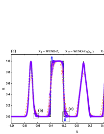
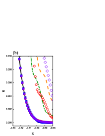
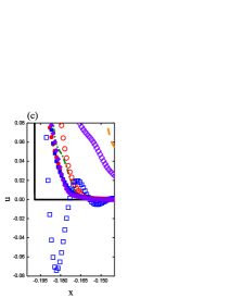
Figure 3: Performance of the considered WENO schemes for SLP (Case 1) at output time $t=200$ with a uniform mesh size of $N=1600$.

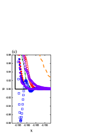
Figure 4: Performance of the considered WENO schemes for SLP (Case 1) at output time $t=200$ with a uniform mesh size of $N=3200$.

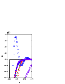
Figure 5: Performance of the considered WENO schemes for BiCWP (Case 2) at output time $t=200$ with a uniform mesh size of $N=1600$.

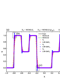
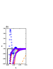
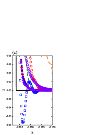
Figure 6: Performance of the considered WENO schemes for BiCWP (Case 2) at output time $t=200$ with a uniform mesh size of $N=3200$.

3.4.2 With high-order critical points

In order to show the advantage of the LOP-GMWENO-X schemes that they can obtain high resolutions for the problem with high-order critical points at long output times, we compute the 1D linear advection equation $u_{t}+u_{x}=0,x\in(3.5,6.5)$ with an initial condition given by $u(x,0)=-\exp\Big{(}-\big{(}x-5.0\big{)}^{10}\Big{)}\cos^{10}\Big{(}\pi\big{(}x-5.0\big{)}\Big{)}$. The CFL number is chosen to be $(\Delta x)^{2/3}$. For convenience, this test is dubbed HCP problem here.

It is trivial to know that the exact solution is $u(x,t)=-\exp\Big{(}-\big{(}(x-t)-5.0\big{)}^{10}\Big{)}\cos^{10}\Big{(}\pi\big{(}(x-t)-5.0\big{)}\Big{)}$. To compare the dissipations, we compute the increased errors, defined by $\chi_{1}=\frac{L_{1}^{\mathrm{Y}}(t)-L_{1}^{\mathrm{ILW}}(t)}{L_{1}^{\mathrm{ILW}}(t)}\times 100\%$ and $\chi_{2}=\frac{L_{2}^{\mathrm{Y}}(t)-L_{2}^{\mathrm{ILW}}(t)}{L_{2}^{\mathrm{ILW}}(t)}\times 100\%$, where $L_{j}^{\mathrm{ILW}}(t)$ and $L_{j}^{\mathrm{Y}}(t)$ stand for the $L_{j}$-norm ($j=1,2$) of numerical errors of the WENO5-ILW scheme and the scheme “Y” respectively.

Table 5 gives the $L_{1}$ and $L_{2}$ errors and the corresponding increased errors computed by various considered WENO schemes with $N=300$ and $t=300,600,900,1200$. For all output times, the WENO-JS scheme generates the largest numerical errors and it produces the highest increased errors. The WENO-Z and WENO-A schemes also have very large numerical errors that are slightly smaller than those of the WENO-JS scheme. Accordingly, the increased errors of these schemes are excessively large. In contrast, the numerical errors and the corresponding increased errors of the associated LOP-GMWENO-Z and LOP-GMWENO-A schemes are significantly reduced to a tolerable level. Actually, they can achieve much smaller numerical errors that get very close to those of the WENO-ILW scheme. In addition, the LOP-GMWENO-Z$\eta(\tau_{81})$ scheme is also able to maintain the numerical errors at an acceptable level to ensure that its increased errors are also at a tolerable level. It appears that the WENO-Z$\eta(\tau_{81})$ schemes gets solutions almost as accurate as, or even more accurate than, those of the WENO-ILW scheme. Of course, this is good, at least for this test. However, as discussed earlier, it suffers from lack of robustness as its dissipation is too small on solving problems with discontinuities, especially for long output time simulations.

Table 5: $L_{1}$-, $L_{2}$-norm of numerical errors and their associated increased errors (in percentage) on solving the HCP problem with $N=300$.

	WENO5-ILW				WENO-JS
Time, $t$	$L_{1}$ error	$\chi_{1}$	$L_{2}$ error	$\chi_{2}$	$L_{1}$ error	$\chi_{1}$	$L_{2}$ error	$\chi_{2}$
300	6.30537E-03	-	5.69915E-03	-	8.88538E-02	1309%	7.58151E-02	1230%
600	1.14068E-02	-	9.89571E-03	-	2.17193E-01	1804%	1.78733E-01	1706%
900	1.58862E-02	-	1.34968E-02	-	2.84952E-01	1694%	2.29984E-01	1604%
1200	1.98304E-02	-	1.65947E-02	-	3.32245E-01	1575%	2.64896E-01	1496%
	WENO-Z				LOP-GMWENO-Z
Time, $t$	$L_{1}$ error	$\chi_{1}$	$L_{2}$ error	$\chi_{2}$	$L_{1}$ error	$\chi_{1}$	$L_{2}$ error	$\chi_{2}$
300	3.56061E-02	465%	3.70325E-02	550%	1.17228E-02	86%	9.94127E-03	74%
600	8.21730E-02	620%	8.66509E-02	776%	2.06455E-02	81%	1.86636E-02	89%
900	1.10948E-01	598%	1.20020E-01	789%	2.88134E-02	81%	2.42690E-02	80%
1200	1.33598E-01	574%	1.30955E-01	689%	3.06112E-02	54%	2.47195E-02	49%
	WENO-Z$\eta(\tau_{81})$				LOP-GMWENO-Z$\eta(\tau_{81})$
Time, $t$	$L_{1}$ error	$\chi_{1}$	$L_{2}$ error	$\chi_{2}$	$L_{1}$ error	$\chi_{1}$	$L_{2}$ error	$\chi_{2}$
300	6.41911E-03	2%	6.41911E-03	13%	1.10215E-02	75%	9.92087E-03	74%
600	1.18436E-02	4%	1.00019E-02	1%	2.03525E-02	78%	1.77994E-02	80%
900	1.65166E-02	4%	1.34843E-02	0%	2.74958E-02	73%	2.29759E-02	70%
1200	2.01696E-02	2%	1.63065E-02	-2%	2.92445E-02	47%	2.45566E-02	48%
	WENO-A				LOP-GMWENO-A
Time, $t$	$L_{1}$ error	$\chi_{1}$	$L_{2}$ error	$\chi_{2}$	$L_{1}$ error	$\chi_{1}$	$L_{2}$ error	$\chi_{2}$
300	1.20889E-01	1817%	1.13688E-01	1895%	1.10467E-02	75%	9.93024E-03	74%
600	1.84388E-01	1516%	1.63149E-01	1549%	2.03180E-02	78%	1.81152E-02	83%
900	1.96326E-01	1136%	1.70146E-01	1161%	2.57805E-02	62%	2.21596E-02	64%
1200	2.12758E-01	973%	1.82152E-01	998%	2.75976E-02	39%	2.35188E-02	42%

In Fig. 7, we plot the $x-u$ profiles of the LOP-GMWENO-X schemes and their associated WENO-X schemes at output time $t=1200$. For the purpose of comparison, we also plot the $x-u$ profiles of the WENO-JS [28] and WENO-M [26] schemes. From Fig. 7, we can intuitively see that the WENO-JS scheme shows the lowest resolution, followed by the WENO-M scheme. As expected, the WENO-Z and WENO-A schemes show very low resolutions. However, the resolutions of the associated LOP-GMWENO-Z and LOP-GMWENO-A schemes have been improved significantly. Although the resolutions are slightly lower than those of its associated WENO-Z$\eta(\tau_{81})$ scheme, the LOP-GMWENO-Z$\eta(\tau_{81})$ scheme still shows far better resolutions than the WENO-JS, WENO-M, WENO-Z and WENO-A schemes.

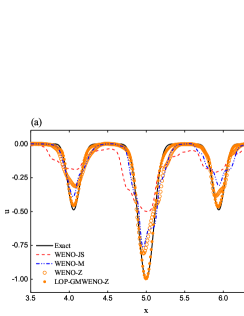
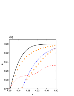
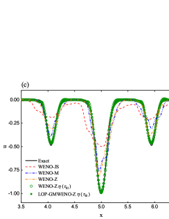
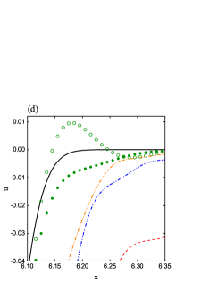
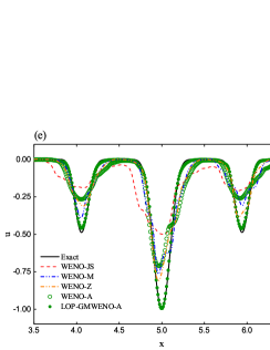
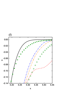
Figure 7: Performance of various WENO schemes for the HCP problem at output time $t=1200$ with a uniform mesh size of $N=300$.

4 Numerical results

In this section, we compare the numerical performance of the considered WENO schemes by solving the system of hyperbolic conservation laws. The governing equations are the following Euler equations

$$\begin{array}[]{l}\begin{aligned} &\dfrac{\partial\rho}{\partial t}+\nabla\cdot(\rho\mathbf{u})=0,\\ &\dfrac{\partial(\rho\mathbf{u})}{\partial t}+\nabla\cdot(\rho\mathbf{u}\mathbf{u}+p\delta)=0,\\ &\dfrac{\partial E}{\partial t}+\nabla\cdot\Big{(}\mathbf{u}(E+p)\Big{)}=0,\end{aligned}\end{array}$$ (17)

where $\rho,\mathbf{u},E,p$ are the density, the velocity vector, the total energy and the pressure. To close this set of equations, the equation of state (EOS) for an ideal polytropic gas $E=\frac{p}{\gamma-1}+\frac{1}{2}\rho\mathbf{u}\mathbf{u}$ with $\gamma=1.4$ as the ratio of specific heats is employed.

The CFL number is set to be $0.5$ for both 1D and 2D problems below (unless otherwise noted), and the global Lax-Friedrichs flux splitting with the local characteristic decomposition [28] is employed. The WENO schemes are applied dimension-by-dimension to solve the two-dimensional Euler system. Zhang et al. [63] proposed two classes of finite volume WENO schemes in two dimension very carefully. For the same reason as discussed in [36], the case of Class A is taken in this paper.

4.1 One-dimensional Euler system

In this subsection, we apply the LOP-GMWENO-X schemes with X = Z, Z$\eta(\tau_{81}),A$, as well as their associated WENO-X schemes, to solve several one-dimensional Euler problems. In order to compare the performance of these schemes with the recently-published low-dissipation shock-capturing ENO-family schemes, say, TENO schemes [15, 16, 12, 13, 17, 7, 14, 21] in terms of the low-dissipation property, the classical TENO5 scheme with the threshold $C_{T}$ as $10^{-5},10^{-3}$ and $10^{-1}$ are considered. We also give the results of the WENO-JS scheme.

4.1.1 Shock-tube problem

To examine the shock-capturing capability of the LOP-GMWENO-X schemes, we compute two widely concerned shock-tube problems, that is, the Sod problem [48] and the Lax problem [31]. The initial conditions are

$$\text{Sod: }\qquad\big{(}\rho,u,p\big{)}(x,0)=\left\{\begin{array}[]{ll}(1.0,0.0,1.0),&x\in[0.0,0.5],\\ (0.125,0.0,0.1),&x\in[0.5,1.0],\end{array}\right.$$

$$\text{Lax: }\qquad\big{(}\rho,u,p\big{)}(x,0)=\left\{\begin{array}[]{ll}(0.445,0.698,3.528),&x\in[-5,0],\\ (0.500,0.000,0.571),&x\in[0,5].\end{array}\right.$$

The transmissive boundary conditions are used, and the output times are 0.25 and 1.3, respectively. In order to compare the performance of the considered schemes on various coarse mesh resolutions, three different mesh sizes of $N=300,900,1500$ are used.

Fig. 8 and Fig. 9 show the computed density profiles of the considered schemes. It is observed that the LOP-GMWENO-Z and LOP-GMWENO-A schemes give results with comparable or slightly lower resolutions than their associated WENO-Z and WENO-A schemes but their resolutions are better than the WENO-JS scheme. The resolution of the LOP-GMWENO-Z$\eta(\tau_{81})$ scheme appears to be lower than its associated WENO-Z$\eta(\tau_{81})$. However, if we take a closer look, we can see that the WENO-Z$\eta(\tau_{81})$ scheme generates spurious oscillations while the LOG-GMWENO-Z$\eta(\tau_{81})$ scheme can avoid the spurious oscillations successfully. Similarly, the TENO5 schemes with the threshold $C_{T}$ as $10^{-5}$ and $10^{-3}$ attain the much higher resolutions than other schemes while they produce very slightly spurious oscillations (a very close look is needed to observe this). One can remove these spurious oscillations by increasing the threshold $C_{T}$. Actually, when $C_{T}=10^{-1}$ is taken, the spurious oscillations have been removed successfully at the price of the loss of resolutions.

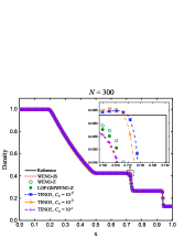
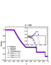
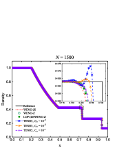
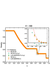
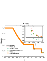
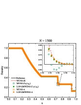
Figure 8: Density plots for the Sod shock-tube problem on various coarse mesh resolutions.

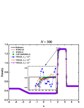
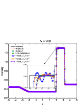
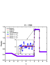
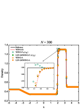
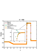
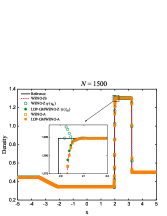
Figure 9: Density plots for the Lax shock-tube problem on various coarse mesh resolutions.

4.1.2 Shock-density wave interaction

To demonstrate the excellent performance of the LOP-GMWENO-X schemes in the region with high-frequency but smooth waves, we simulate two typical shock-density wave interaction problems, that is, the Shu-Osher problem [47] and the Titarev-Toro problem [49, 51, 50]. The initial conditions are

Shu-Osher: $$\big{(}\rho,u,p\big{)}(x,0)=\left\{\begin{array}[]{ll}(3.857143,2.629369,10.333333),&x\in[-5.0,-4.0],\\ (1.0+0.2\sin(5x),0,1),&x\in[-4.0,5.0],\end{array}\right.$$

Titarev-Toro: $$\big{(}\rho,u,p\big{)}(x,0)=\left\{\begin{array}[]{ll}(1.515695,0.5233346,1.80500),&x\in[-5.0,-4.5],\\ (1.0+0.1\sin(20\pi x),0,1),&x\in[-4.5,5.0].\end{array}\right.$$

The transmissive boundary conditions are used at $x=\pm 5$. The output times are set to be 1.8 and 5.0, and the uniform mesh sizes of $N=300$ and $N=1500$ are used for the Shu-Osher problem and the Titarev-Toro problem, respectively.

The solutions of density of the LOP-GMWENO-Z, LOP-GMWENO-Z$\eta(\tau_{81})$, LOP-GMWENO-A schemes, as well as their associated WENO-Z, WENO-Z$\eta(\tau_{81})$, WENO-A schemes, are given in Fig. 10 and Fig. 11, where the reference solutions are computed by employing WENO-JS with $N=10000$. Again, for comparison purpose, we show the solutions of the aforementioned TENO5 schemes and that of WENO-JS. As shown in Fig. 10, for the Shu-Osher problem, the LOP-GMWENO-Z, LOP-GMWENO-Z$\eta(\tau_{81})$ and LOP-GMWENO-A schemes provide comparable results with those of their associated WENO-Z, WENO-Z$\eta(\tau_{81})$ and WENO-A schemes which are far better than that of the WENO-JS scheme, and the TENO5 schemes with the threshold $C_{T}$ as $10^{-5}$ and $10^{-3}$ enjoy higher resolutions because of their low-dissipation property. As expected, when $C_{T}=10^{-1}$ is taken, its resolution decreases to the same or slightly lower level of the LOP-GMWENO-Z scheme. For the Titarev-Toro problem, from Fig. 11, we can find that the LOP-GMWENO-Z, LOP-GMWENO-Z$\eta(\tau_{81})$ and LOP-GMWENO-A schemes achieve much higher resolutions than their associated WENO-Z, WENO-Z$\eta(\tau_{81})$ and WENO-A schemes. Moreover, the considered TENO5 schemes can obtain better resolutions than the WENO-Z scheme, while their resolutions are evidently lower than those of all the considered LOP-GMWENO-X schemes.

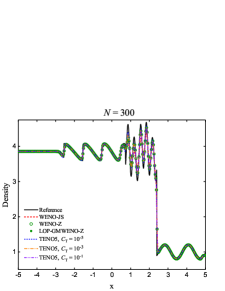
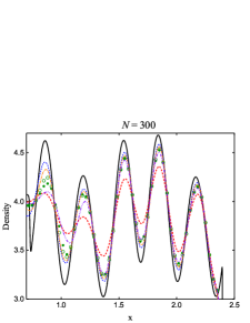
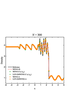
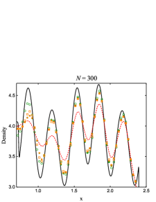
Figure 10: Density plots for the Shu-Osher shock-density wave interaction problem.

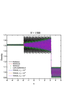
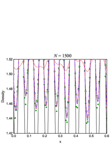
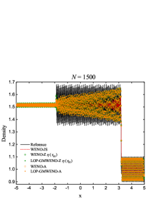
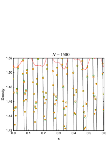
Figure 11: Density plots for the Titarev-Toro shock-density wave interaction problem.

4.2 Two-dimensional Euler system

In this subsection, we present numerical experiments with the two-dimensional Euler equations, such as the accuracy tests for smooth problems, 2D interacting blast waves problem, implosion and explosion problems, shock-vortex interaction (SVI) problem, regular shock reflection (RSR) problem, double Mach reflection (DMR) problem, forward facing step (FFS) problem and Rayleigh-Taylor instability (RTI) problem.

4.2.1 Accuracy test for 2D smooth Euler problems

We solve the 2D smooth Euler problem on the computational domain $[-1.0,1.0]\times[-1.0,1.0]$ to demonstrate the convergence property of the present scheme, and the density wave propagation problem [29] with the following two initial conditions are calculated

Case 1: $$(\rho,u,v,p)(x,y,0)=\Big{(}1.0+0.2\sin\big{(}\pi(x+y)\big{)},0.7,0.3,1.0\Big{)},$$ (18)

Case 2: $$(\rho,u,v,p)(x,y,0)=\Bigg{(}1.0+0.2\sin\bigg{(}\pi(x+y)-\dfrac{\sin(\pi(x+y))}{\pi}\bigg{)},0.7,0.3,1.0\Bigg{)}.$$

The periodic boundary condition is used. We set $h=h_{x}=h_{y}$ in all calculations of this paper with $h_{x},h_{y}$ as the uniform spatial step size in $x$- and $y$- direction. The CFL number is set to be $h^{2/3}$ so that the error for the overall scheme is a measure of the spatial convergence only. The calculation is advanced to $t=2$.

To test the convergence orders, the following $L_{\infty}$-norm error of the density is computed

$$L_{\infty}=\max_{\begin{subarray}{c}1\leq i\leq N_{x}\\ 1\leq j\leq N_{y}\end{subarray}}\Big{\lvert}\rho_{i,j}^{\mathrm{exact}}-(\rho_{h})_{i,j}\Big{\rvert},$$

where $N_{x},N_{y}$ is the number of cells in $x-$ and $y-$ direction. $(\rho_{h})_{i,j}$ is the numerical solution of the density and $\rho_{i,j}^{\mathrm{exact}}$ is its exact solution.

For comparison purpose, we also apply the aforementioned TENO5 schemes and the WENO-JS scheme to this accuracy test. In Fig. 12, we provide the overall $L_{\infty}$ convergence behavior of all considered schemes. Obviously, as evidenced by the slope of the profiles, all the LOP-GMWENO-X schemes and their associated WENO-X schemes, as well as the TENO5 schemes with the threshold $C_{T}$ as $10^{-5},10^{-3},10^{-1}$, can recover the optimal convergence orders for both Case 1 and Case 2. Although the WENO-JS scheme can also obtain the optimal convergence order for Case 1, it can only achieve third-order convergence rate of accuracy for Case 2. Moreover, in terms of accuracy, the results of the LOP-GMWENO-X schemes are almost identical to those of the associated WENO-X schemes and the TENO5 schemes, and all these schemes have much smaller numerical errors than the WENO-JS scheme.

In order to examine the efficiency of Algorithm 1 , we plot the graphs for the CPU time versus the $L_{\infty}$-norm errors in Fig. 13. Generally speaking, the LOP-GMWENO-X schemes have comparable or very slightly lower efficiency in comparison with their associated WENO-X schemes and the TENO5 schemes. Clearly, the efficiency of the LOP-GMWENO-X schemes are much higher than that of the WENO-JS scheme.

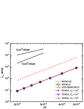
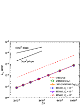
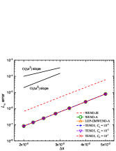
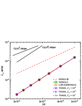
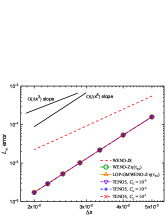
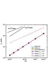
Figure 12: Convergence of the $L_{\infty}$-norm errors of various WENO schemes for 2D smooth Euler problems. Top: Case 1. Bottom: Case 2.

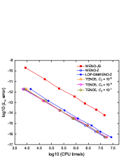
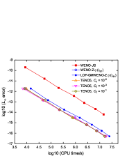
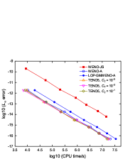
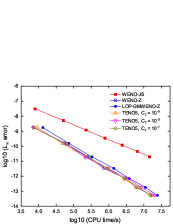
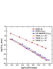
Figure 13: CPU-time versus $L_{\infty}$-norm errors of various WENO schemes for 2D smooth Euler problems. Top: Case 1. Bottom: Case 2.

4.2.2 2D interacting blast waves

We solve the 2D version of the standard blast-wave interaction problem first used by Woodward and Colella [58]. The computational domain $[0,1]\times[0,0.4]$ is initialized by

$$\big{(}\rho,u,v,p\big{)}(x,y,0)=\left\{\begin{array}[]{ll}(1,0,0,1000),&x\in[0,0.1),y\in[0,0.4]\\ (1,0,0,0.01),&x\in[0.1,0.9),y\in[0,0.4]\\ (1,0,0,100),&x\in[0.9,1.0],y\in[0,0.4].\end{array}\right.$$

The reflective boundary conditions are used at $x=0,1$ and the zero-gradient boundary conditions are used at $y=0,0.4$. The output time is 0.038, and the uniform mesh of $N_{x}\times N_{y}=300\times 120$ is used.

In Fig. 14, the density contours and the density profiles at plane $y=0.2$ of the LOP-GMWENO-Z, LOP-GMWENO-Z$\eta(\tau_{5})$, LOP-GMWENO-A schemes and their associated WENO-Z, WENO-Z$\eta(\tau_{5})$, WENO-A schemes are presented. For comparison purpose, we also plot the density profiles of the WENO-JS scheme and the reference result is obtained by solving the corresponding 1D case using the WENO-JS scheme with $N=10000$. It can be seen that the LOP-GMWENO-X schemes perform as well as their associated WENO-X schemes, and all of these schemes generate sharper results than the WENO-JS scheme. It should be noted that we present the result of the WENO-Z$\eta(\tau_{5})$ scheme but not that of the WENO-Z$\eta(\tau_{81})$ scheme in this test as it was indicated [9] that simulations under the use of WENO-Z$\eta(\tau_{81})$ scheme is found to be unstable.

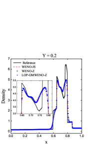
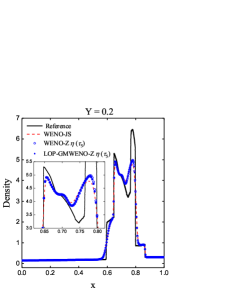
Figure 14: Solutions of the interacting blast waves problem. Top: density contours. Bottom: density profiles at plane $y=0.2$.

4.2.3 Implosion and explosion problems

We simulate the implosion problem [59] and explosion problem [33, 52]. In order to examine the performance for a long-time run, we reset the computational domain of the explosion problem used in [33, 52] to be $[-10,10]\times[-10,10]$ and the output time to be $t=5.0$. For the implosion problem, we use the same computational domain of $[-20,20]\times[-20,20]$ as in [59] where a large output time $t=4.2$ was used. The initial conditions are given as

Implosion: $$\big{(}\rho,u,v,p\big{)}(x,y,0)=\left\{\begin{array}[]{ll}(1,0,0,1),&\mathrm{if}\sqrt{x^{2}+y^{2}}<0.4,\\ (0.125,0,0,0.1),&\mathrm{else},\end{array}\right.$$

Explosion: $$\big{(}\rho,u,v,p\big{)}(x,y,0)=\left\{\begin{array}[]{ll}(2,0,0,5),&\mathrm{if}\sqrt{x^{2}+y^{2}}<4.0,\\ (1,0,0,1),&\mathrm{else}.\end{array}\right.$$

On all edges, the reflective boundary condition is used for the implosion problem, and the transmissive boundary condition is used for the explosion problem. $N_{x}\times N_{y}=400\times 400$ is used for these two problems.

In Fig. 15 and Fig. 16, the density contours (the first two columns) and the desity profiles at plane $y=0.0$ (the last column) of the LOP-GMWENO-Z, LOP-GMWENO-Z$\eta(\tau_{81})$ and LOP-GMWENO-A schemes, as well as their associated WENO-Z, WENO-Z$\eta(\tau_{81})$ and WENO-A schemes, are presented respectively. We also show the results of the WENO-JS scheme in the desity profiles (see the last column) where the reference solutions are computed by the WENO-JS scheme with $N_{x}\times N_{y}=1000\times 1000$. We can see that all considered schemes can successfully capture the main structures of the implosion and explosion problems. Moreover, for the implosion problem, as shown in the last column of Fig. 15, the solutions of the LOP-GMWENO-Z and LOP-GMWENO-A schemes are very close to those of their associated WENO-Z and WENO-A schemes respectively, while the LOP-GMWENO-Z$\eta(\tau_{81})$ scheme has a lower resolution than the WENO-Z$\eta(\tau_{81})$ scheme. Similarly, for the explosion problem, as shown in the last column of Fig. 16, the solutions of the LOP-GMWENO-Z and LOP-GMWENO-Z$\eta(\tau_{81})$ schemes are very close to those of their associated WENO-Z and WENO-Z$\eta(\tau_{81})$ schemes respectively, and the resolution of the LOP-GMWENO-A scheme appears to be higher than the WENO-A scheme. As expected, the WENO-JS scheme produces lower resolutions than all other considered schemes.

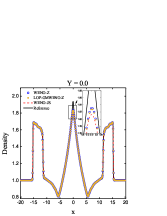
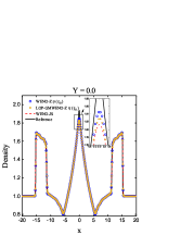
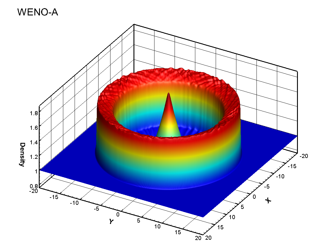
Figure 15: Solutions of the 2D implosion problem. Left and middle: density contours. Right: density profiles at plane $y=0.0$.

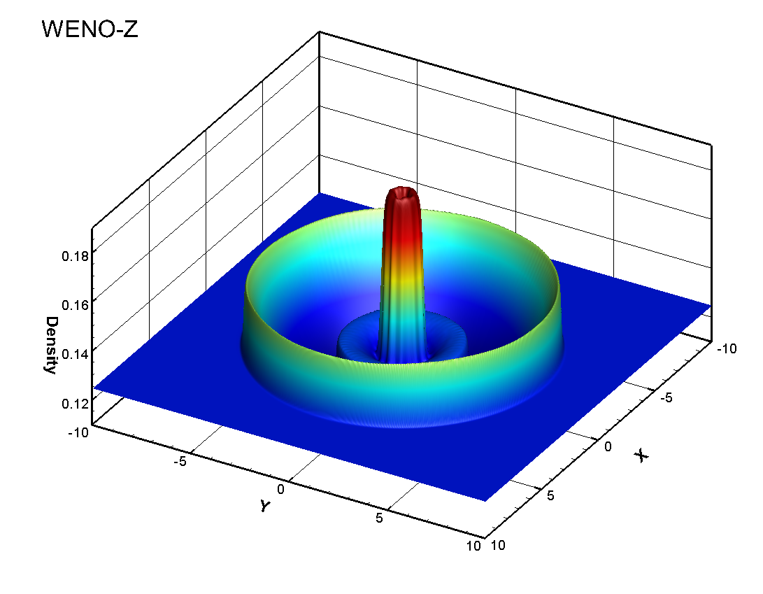
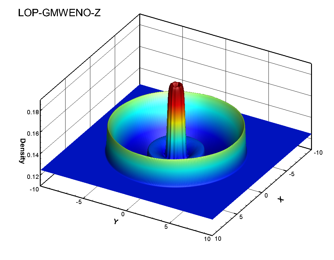
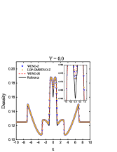
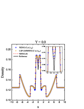
Figure 16: Solutions of the 2D explosion problem. Left and middle: density contours. Right: density profiles at plane $y=0.0$.

4.2.4 Shock-vortex interaction

The shock-vortex interaction problem is widely used to examine the performance of the high-resolution methods [5, 41, 42]. The computational domain is $[0,1]\times[0,1]$ and it is initialized by

$$\big{(}\rho,u,v,p\big{)}(x,y,0)=\left\{\begin{aligned} \begin{array}[]{ll}\bf{U}_{\mathrm{L}},&x<0.5,\\ \bf{U}_{\mathrm{R}},&x\geq 0.5,\\ \end{array}\end{aligned}\right.$$

where ${\bf{U}}_{\mathrm{L}}=\big{(}\rho_{\mathrm{L}}+\delta\rho,u_{\mathrm{L}}+\delta u,v_{\mathrm{L}}+\delta v,p_{\mathrm{L}}+\delta p\big{)}$ and ${\bf{U}}_{\mathrm{R}}=\big{(}\rho_{\mathrm{R}},u_{\mathrm{R}},v_{\mathrm{R}},p_{\mathrm{R}}\big{)}$, with

$$\begin{array}[]{l}\begin{aligned} &\rho_{\mathrm{L}}=1,\qquad u_{\mathrm{L}}=\sqrt{\gamma},\qquad v_{\mathrm{L}}=0,\qquad p_{\mathrm{L}}=1,\\ &\rho_{\mathrm{R}}=\rho_{\mathrm{L}}\bigg{(}\dfrac{\gamma-1+(\gamma+1)p_{\mathrm{R}}}{\gamma+1+(\gamma-1)p_{\mathrm{R}}}\bigg{)},u_{\mathrm{R}}=u_{\mathrm{L}}\bigg{(}\dfrac{1-p_{\mathrm{R}}}{\sqrt{\gamma-1+p_{\mathrm{R}}(\gamma+1)}}\bigg{)},v_{\mathrm{R}}=0,p_{\mathrm{R}}=1.3,\\ &\delta\rho=\dfrac{\rho_{\mathrm{L}}^{2}}{(\gamma-1)p_{\mathrm{L}}}\delta T,\delta u=\epsilon\dfrac{y-y_{\mathrm{c}}}{r_{\mathrm{c}}}\mathrm{e}^{\alpha(1-r^{2})},\delta v=-\epsilon\dfrac{x-x_{\mathrm{c}}}{r_{\mathrm{c}}}\mathrm{e}^{\alpha(1-r^{2})},\delta p=\dfrac{\gamma\rho_{\mathrm{L}}^{2}}{(\gamma-1)\rho_{\mathrm{L}}}\delta T,\end{aligned}\end{array}$$

and $\epsilon=0.3,r_{\mathrm{c}}=0.05,\alpha=0.204,x_{\mathrm{c}}=0.25,y_{\mathrm{c}}=0.5,r=\sqrt{((x-x_{\mathrm{c}})^{2}+(y-y_{\mathrm{c}})^{2})/r_{\mathrm{c}}^{2}},\delta T=-(\gamma-1)\epsilon^{2}\mathrm{e}^{2\alpha(1-r^{2})}/(4\alpha\gamma)$. The transmissive boundary condition is used on all edges. The computational domain is discretized into $800\times 800$ uniform cells, and the calculations are advanced in time up to $t=0.6$.

We consider the LOP-GMWENO-X schemes with X = Z, Z$\eta(\tau_{81})$, A and their associated WENO-X schemes (hereinafter the same). Fig. 17 gives the solutions computed by all considered WENO schemes, and the main structure of the shock and vortex after the interaction are properly captured by all considered schemes. Fig. 18 presents the zoomed-in view to show the numerical oscillations more clearly. It indicates that the WENO-X schemes generate severe post-shock oscillations while their associated LOP-GMWENO-X schemes can significantly decrease these oscillations. In order to demonstrate this more clearly, in Fig. 19, we give the cross-sectional slices of density plot along the plane $y=0.30$ in $x\in(0.44,0.54)$ where the reference solution is obtained using the WENO-JS scheme with a uniform mesh size of $1600\times 1600$. Of course, the LOP-GMWENO-X schemes can not thoroughly remove the numerical oscillations. However, it is obvious that they can significantly reduce these oscillations compared to their associated WENO-X schemes. Indeed, this is a huge improvement for the WENO-Z$\eta(\tau_{81})$ and WENO-A schemes on reducing the post-shock oscillations, and the improvement for the WENO-Z scheme is also noticeable. Therefore, we conclude that this should be an additional advantage of the WENO-Z-type schemes with LOP generalized mappings.

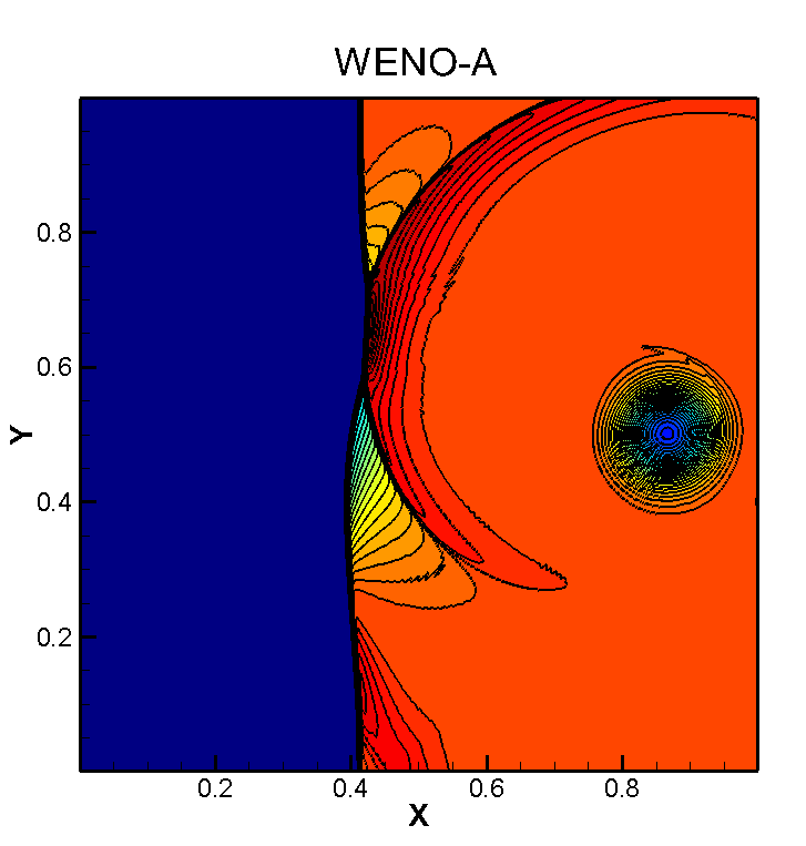
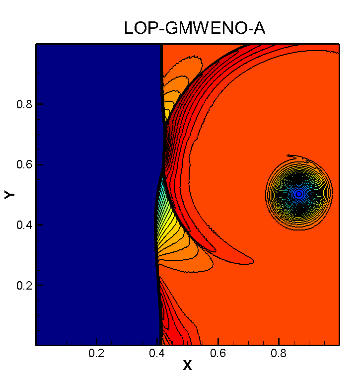
Figure 17: Density plots for the Shock-vortex interaction using $50$ contour lines with range from $1.0$ to $2.7$.

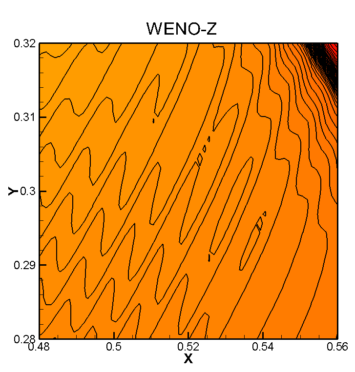
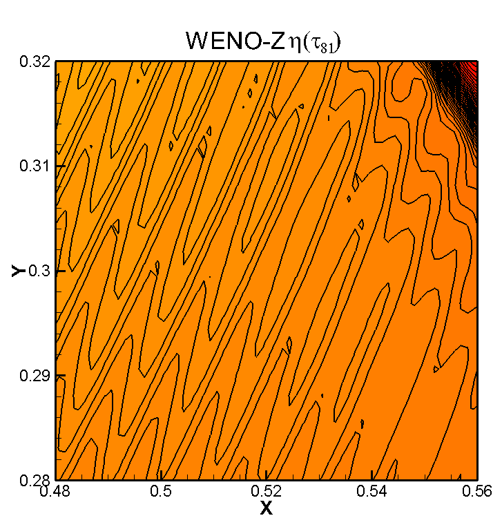
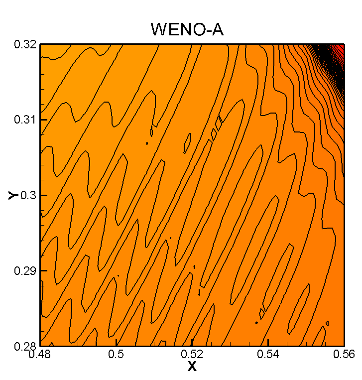
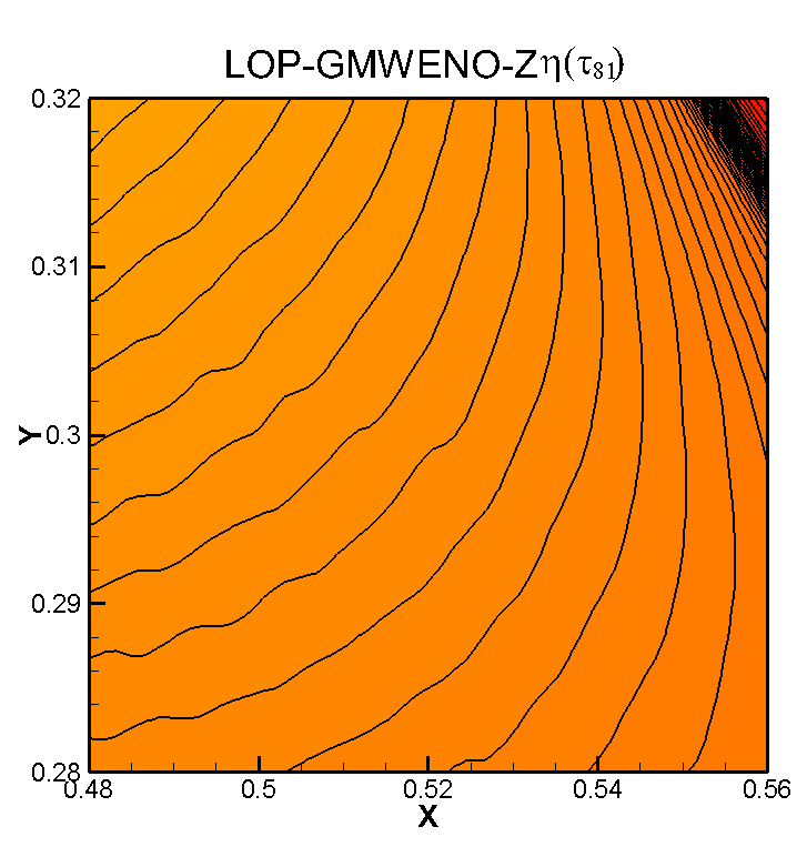
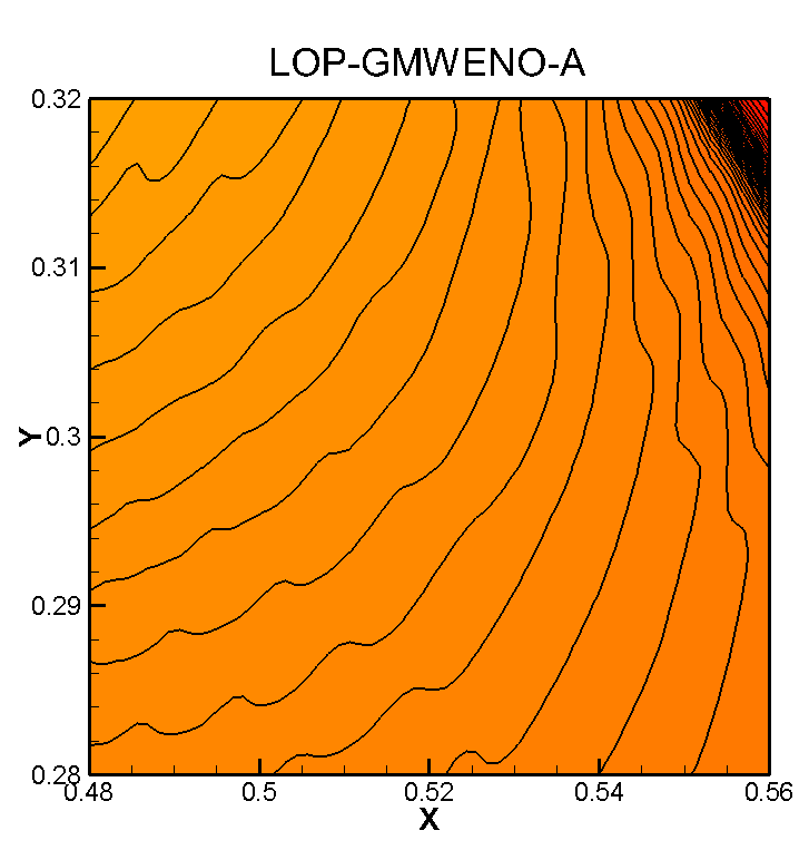
Figure 18: The zoomed-in density plots using $400$ contour lines with range from $1.0$ to $2.7$.

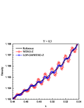
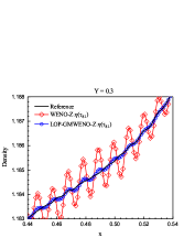
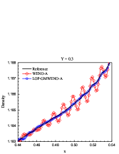
Figure 19: The cross-sectional slices of density plot along the plane $y=0.30$ where $x\in[0.44,0.54]$.

4.2.5 Regular shock reflection

As used in [64], we simulate the regular shock reflection. This is a typical 2D steady flow. The computational domain is a rectangle of 4 length units times 1 length unit, say, $[0,4]\times[0,1]$ here. It is initialized by

$$\big{(}\rho,u,v,p\big{)}(x,y,0)=(1.0,2.9,0.0,1.0/\gamma),$$

where $\gamma=1.4$. Along the bottom and the right edges, the reflection and transmissive boundary conditions are used respectively. The following Dirichlet boundary conditions are used along the top and left edges

$$\big{(}\rho,u,v,p\big{)}(x,y,t)=\left\{\begin{array}[]{ll}(1.69997,2.61934,-0.50632,1.52819),&\text{where}\quad y=1,\\ (1.0,2.9,0.0,1.0/\gamma),&\text{where}\quad x=0.\end{array}\right.$$

A uniform mesh size of $800\times 200$ is used and the final time is $t=2.5$.

In Fig. 20, we show the density contours computed by the LOP-GMWENO-X schemes (the right column) and their associated WENO-X schemes (the left column). In general, all the considered schemes can capture the main structure of the shock transitions for this problem. Unfortunately, all these schemes produce the post-shock numerical oscillations. However, in comparison with the WENO-X schemes without LOP, their associated LOP-GMWENO-X schemes can significantly reduce these oscillations. In order to more clearly manifest this, we show the cross-sectional slices of density plot along the plane $y=0.5$ in $x\in(0.9,1.1)$ in Fig. LABEL:fig:ex:RSR:2. For comparison purpose, we also plot the results of the WENO-ZS [64] scheme using two different mesh sizes of $N_{x}\times N_{y}=800\times 200,1600\times 400$. It is well known that WENO-ZS is able to either remove or significantly reduce the post-shock oscillations. It can easily be found that the post-shock oscillations produced by the WENO-X schemes are much severer than those of their associated LOP-GMWENO-X schemes. In other words, the post-shock oscillations of the LOP-GMWENO-X schemes are considerably reduced compared to those of their associated WENO-X schemes. As mentioned before, this should be an advantage of the WENO-Z-type schemes with LOP mappings. Furthermore, although the post-shock oscillations generated by the LOP-GMWENO-X schemes are slightly severer than that of the WENO-ZS scheme, the LOP-GMWENO-X schemes achieve higher resolutions than the WENO-ZS scheme under the same mesh resolution. Indeed, the resolutions of the LOP-GMWENO-X schemes with $N_{x}\times N_{y}=800\times 200$ is comparable to that of WENO-ZS with $N_{x}\times N_{y}=1600\times 400$. In summary, this might be another additional advantage of the LOP-GMWENO-X schemes in some ways.

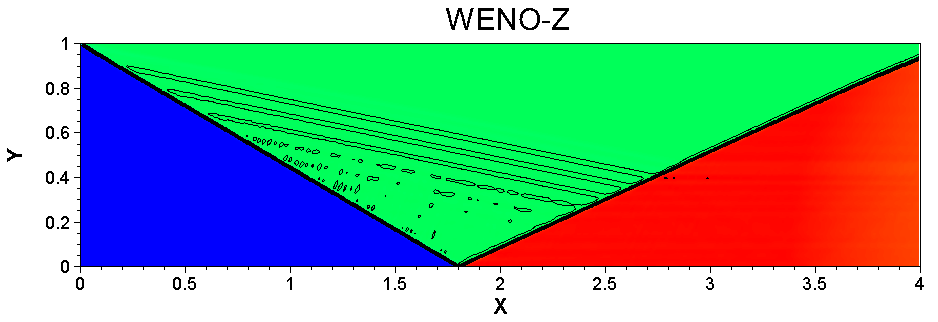
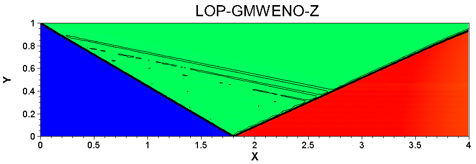
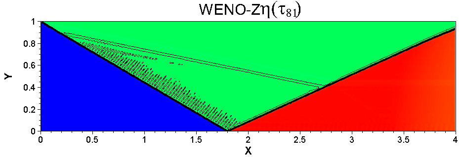
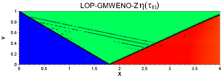
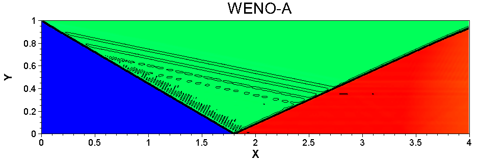
Figure 20: Density plots for the regular shock reflection using $30$ contour lines with range from $1.05$ to $2.7$.

4.2.6 Double Mach reflection of a strong shock

This problem was initially proposed by Woodward and Colella [58]. The computational domain is set to be $[0,4]\times[0,1]$ and it is initialized by

$$\big{(}\rho,u,v,p\big{)}(x,y,0)=\left\{\begin{aligned} \begin{array}[]{ll}(8.0,8.25\cos\theta,-8.25\sin\theta,116.5),&x<x_{0}+\dfrac{y}{\sqrt{3}},\\ (1.4,0.0,0.0,1.0),&x\geq x_{0}+\dfrac{y}{\sqrt{3}},\\ \end{array}\end{aligned}\right.$$

where $\theta=\frac{\pi}{6}$ and $x_{0}=\frac{1}{6}$. The inflow boundary condition with the post-shock values as stated above and the outflow boundary condition are used at $x=0$ and $x=4$ respectively. At $y=0$, the post-shock values are imposed at $[0,x_{0})$, while the reflective boundary condition is applied to $[x_{0},4]$. At $y=1$, the fluid variables are defined as to the exact solution of the Mach 10 moving oblique shock. The uniform meshes of $N_{x}\times N_{y}=2000\times 500$ and the output time $t=0.2$ are used.

Fig. LABEL:fig:ex:DMR illustrates the results from the LOP-GMWENO-Z, LOP-GMWENO-Z$\eta(\tau_{81})$, LOP-GMWENO-A schemes and their associated WENO-Z, WENO-Z$\eta(\tau_{81})$, WENO-A schemes. All these schemes can properly give the main structure of the flow field and successfully capture the companion structure and the small vortices generated along the slip lines. In addition, they have resolved much richer vortical structures than the WENO-JS schemes whose solution at the same grid space can be found in [33]. Closer inspection of Fig. LABEL:fig:ex:DMR shows that the LOP-GMWENO-Z and LOP-GMWENO-A schemes can slightly decrease the numerical oscillations of their associated WENO-Z and WENO-A schemes.

4.2.7 Forward facing step problem

In recent studies, this benchmark problem originally presented by Woodward and Colella [58] have been widely used to test the performances of various high order schemes [3, 2, 9, 34, 33]. Its setup is as follows: a step with a height of $0.2$ length units located $0.6$ length units from the left-hand end of a wind tunnel, which is $1$ length unit wide and $3$ length units long. The computational domain of this problem is $\Omega=[0,0.6]\times[0,1]\cup[0.6,3]\times[0.2,1]$ and it is initialized by

$$\big{(}\rho,u,v,p\big{)}(x,y,0)=(1.4,3.0,0.0,1.0),\quad(x,y)\in\Omega.$$

Reflective boundary conditions are applied along the walls of the wind tunnel and the step. At the left and right boundaries, inflow and outflow conditions are applied respectively. The mesh resolution is $900\times 300$.

Fig. 23 shows the density contours of the LOP-GMWENO-Z, LOP-GMWENO-Z$\eta(\tau{81})$, LOP-GMWENO-A schemes and their associated WENO-Z, WENO-Z$\eta(\tau{81})$, WENO-A schemes at the final time $t=4.0$. We can see that all these schemes can simulate the complicated structure of the flow field successfully.

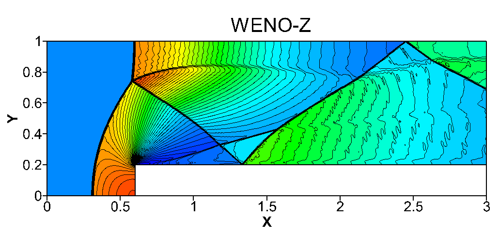
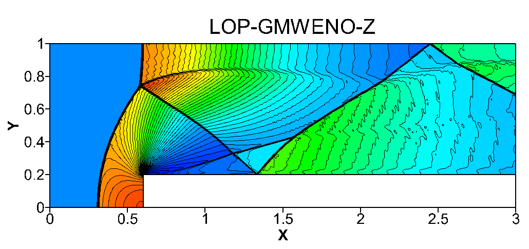
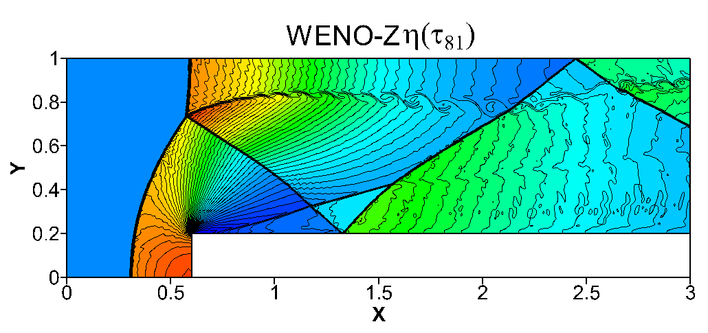
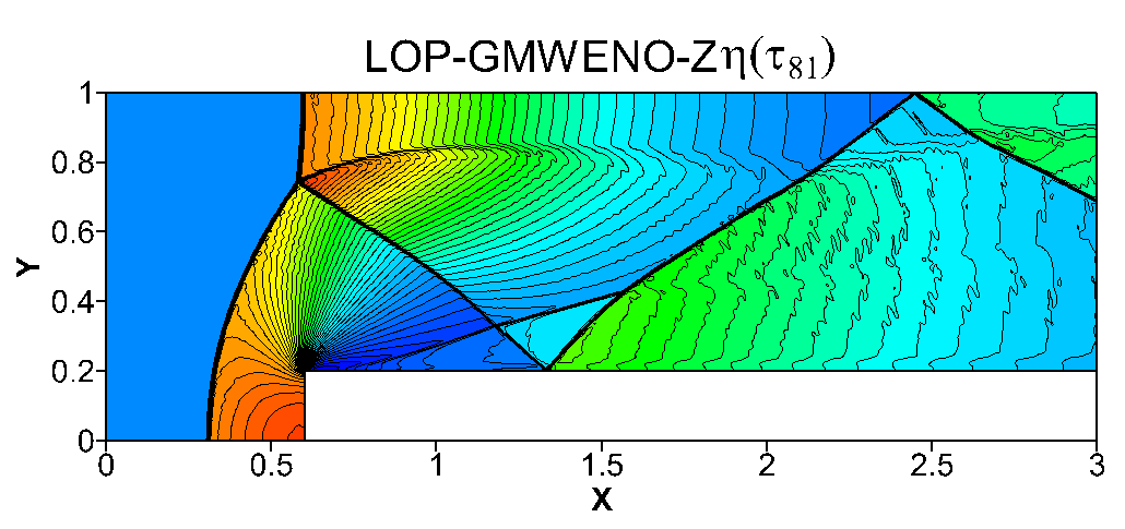
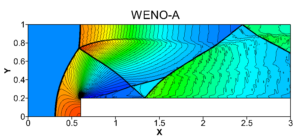
Figure 23: Density contours for the forward facing step problem at output time $t=4.0$ with a uniform mesh size of $900\times 300$.

4.2.8 Rayleigh-Taylor instability

The inviscid Rayleigh-Taylor instability problem used in [44, 60] is computed here. The computational domain is set to be $[0,1/4]\times[0,1]$ and it is initialized by

$$\big{(}\rho,u,v,p\big{)}(x,y,0)=\left\{\begin{aligned} \begin{array}[]{ll}(2,0,-0.025c\cdot\cos(8\pi x),2y+1),&y\leq 0.5,\\ (1,0,-0.025c\cdot\cos(8\pi x),y+1.5),&y>0.5,\end{array}\end{aligned}\right.$$

where the speed of sound is $c=\sqrt{\gamma p/\rho}$ with the ratio of specific heats of $\gamma=5/3$. At $x=0$ and $x=0.25$, the reflective boundary conditions are used. At $y=0$ and $y=1$, the following Dirichlet boundary conditions are imposed

$$\begin{array}[]{l}\big{(}\rho,u,v,p\big{)}(x,y,t)=\left\{\begin{array}[]{ll}(2,0,0,1),&y=0,\\ (1,0,0,2.5),&y=1.\end{array}\right.\end{array}$$

Fig. 24 shows the numerical results of all comsidered WENO schemes at a spatial resolution $N_{x}\times N_{y}=240\times 960$ with the output time $t=1.98$. Clearly, the LOP-GMWENO-Z, LOP-GMWENO-Z$\eta(\tau_{81})$, LOP-GMWENO-A schemes and their associated WENO-Z, WENO-Z$\eta(\tau_{81})$, WENO-A schemes produce finer structures than the WENO-JS scheme. Furthermore, the LOP-GMWENO-Z, LOP-GMWENO-Z$\eta(\tau_{81})$, LOP-GMWENO-A schemes include more noticeable flow asymmetry than their associated WENO-Z, WENO-Z$\eta(\tau_{81})$, WENO-A schemes, and it has been indicated [12] that the low-dissipation property tends to break the flow symmetry, and in other words [15], a more dissipative scheme is more likely to prevent this asymmetry.

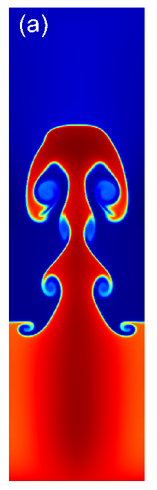
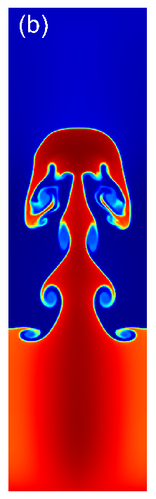
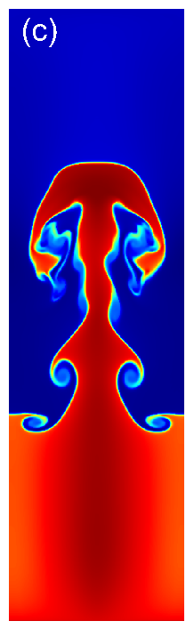
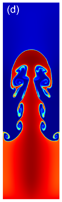
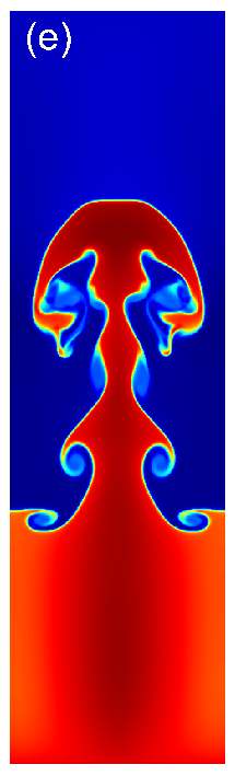
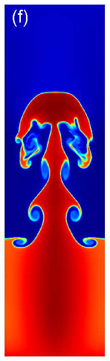
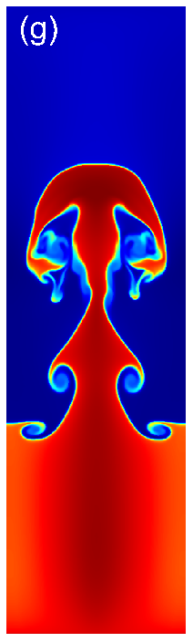
Figure 24: Solutions of the Rayleigh–Taylor instability problem: (a) WENO-JS, (b) WENO-Z, (c) LOP-GMWENO-Z, (d) WENO-Z$\eta(\tau_{81})$, (e) LOP-GMWENO-Z$\eta(\tau_{81})$, (f) WENO-A, (g) LOP-GMWENO-A.

5 Conclusions

In this paper, we investigate extending the order-preserving (OP) criterion to the WENO-Z-type schemes. The locally order-preserving (LOP) mapping is introduced resulting in the improved WENO-Z-type schemes, dubbed LOP-GMWENO-X. The major advantages of the new LOP-GMWENO-X schemes are in fourfolds. Firstly and most importantly, they can successfully remove spurious oscillations and meanwhile obtain high resolutions for long simulations of hyperbolic problems with discontinuities while their associated WENO-Z-type schemes can not. Secondly, on solving hyperbolic problems with high-order critical points for long output times, they can achieve considerable high resolution. Thirdly, in the region with high-frequency but smoothwaves, they can get evidently higher resolution than their associated WENO-Z-type schemes. And lastly, their post-shock oscillations of the 2D Euler problems with strong shock waves are much less and smaller than those of their counterpart WENO-Z-type schemes. Extensive numerical experiments have been performed to demonstrate these advantages. The numerical tests also show that the new schemes can achieve designed convergence orders in smooth regions even in the presence of critical points.

References

- Acker et al. [2016] F. Acker, R.B.d.R. Borges, C. B., An improved WENO-Z scheme, J. Comput. Phys. 313 (2016) 726–753.
- Balsara et al. [2013] D.S. Balsara, C. Meyer, M. Dumbser, H. Du, Z. Xu, Efficient implementation of ADER schemes for Euler and magnetohydrodynamical flows on structured meshes - Speed comparisons with Runge-Kutta methods, J. Comput. Phys. 235 (2013) 934–969.
- Balsara et al. [2009] D.S. Balsara, T. Rumpf, M. Dumbser, C.D. Munz, Efficient, high accuracy ADER-WENO schemes for hydrodynamics and divergence-free magnetohydrodynamics, J. Comput. Phys. 228 (2009) 2480–2516.
- Borges et al. [2008] R. Borges, M. Carmona, B. Costa, W.S. Don, An improved weighted essentially non-oscillatory scheme for hyperbolic conservation laws, J. Comput. Phys. 227 (2008) 3191–3211.
- Chatterjee [1999] A. Chatterjee, Shock wave deformation in shock-vortex interactions, Shock Waves 9 (1999) 95–105.
- Chen et al. [2021] J. Chen, X. Cai, J. Qiu, J.M. Qiu, Adaptive Order WENO Reconstructions for the Semi-Lagrangian Finite Difference Scheme for Advection Problem, Commun. Comput. Phys. 30 (2021) 67–96.
- Dong et al. [2019] H. Dong, L. Fu, F. Zhang, Y. Liu, J. Liu, Detonation Simulations with a Fifth-Order TENO Scheme, Commun. Comput. Phys. 25 (2019) 1357–1393.
- Fan [2014] P. Fan, High order weighted essentially non-oscillatory WENO- schemes for hyperbolic conservation laws, J. Comput. Phys. 269 (2014) 355–385.
- Fan et al. [2014] P. Fan, Y. Shen, B. Tian, C. Yang, A new smoothness indicator for improving the weighted essentially non-oscillatory scheme, J. Comput. Phys. 269 (2014) 329–354.
- Feng et al. [2012] H. Feng, F. Hu, R. Wang, A new mapped weighted essentially non-oscillatory scheme, J. Sci. Comput. 51 (2012) 449–473.
- Feng et al. [2014] H. Feng, C. Huang, R. Wang, An improved mapped weighted essentially non-oscillatory scheme, Appl. Math. Comput. 232 (2014) 453–468.
- Fu [2019a] L. Fu, A low-dissipation finite-volume method based on a new TENO shock-capturing scheme, Comput. Phys. Commun. 235 (2019a) 25–39.
- Fu [2019b] L. Fu, A very-high-order TENO scheme for all-speed gas dynamics and turbulence, Comput. Phys. Commun. 244 (2019b) 117–131.
- Fu [2021] L. Fu, Very-high-order TENO schemes with adaptive accuracy order and adaptive dissipation control, Comput. Meth. Appl. Mech. Eng. 387 (2021) 114193.
- Fu et al. [2016] L. Fu, X.U. Hu, N.A. Adams, A family of high-order targeted ENO schemes for compressible-fluid simulations, J. Comput. Phys. 305 (2016) 333–359.
- Fu et al. [2018] L. Fu, X.U. Hu, N.A. Adams, A new class of adaptive high-order targeted ENO schemes for hyperbolic conservation laws, J. Comput. Phys. 374 (2018) 724–751.
- Fu and Tang [2019] L. Fu, Q. Tang, High-Order Low-Dissipation Targeted ENO Schemes for Ideal Magnetohydrodynamics, J. Sci. Comput. 80 (2019) 692–716.
- Gottlieb and Shu [1998] S. Gottlieb, C.W. Shu, Total variation diminishing Runge-Kutta schemes, Math. Comput. 67 (1998) 73–85.
- Gottlieb et al. [2001] S. Gottlieb, C.W. Shu, E. Tadmor, Strong stability-preserving high-order time discretization methods, SIAM Rev. 43 (2001) 89–112.
- Ha et al. [2013] Y. Ha, C.H. Kim, Y.J. Lee, J. Yoon, An improved weighted essentially non-oscillatory scheme with a new smoothness indicator, J. Comput. Phys. 232 (2013) 68–86.
- Haimovich and Frankel [2017] O. Haimovich, S.H. Frankel, Numerical simulations of compressible multicomponent and multiphase flow using a high-order targeted ENO (TENO) finite-volume method, Comput. Fluids 146 (2017) 105–116.
- Harten [1989] A. Harten, ENO schemes with subcell resolution, J. Comput. Phys. 83 (1989) 148–184.
- Harten et al. [1987] A. Harten, B. Engquist, S. Osher, S.R. Chakravarthy, Uniformly high order accurate essentially non-oscillatory schemes III, J. Comput. Phys. 71 (1987) 231–303.
- Harten and Osher [1987] A. Harten, S. Osher, Uniformly high order accurate essentially non-oscillatory schemes I, SIAM J. Numer. Anal. 24 (1987) 279–309.
- Harten et al. [1986] A. Harten, S. Osher, B. Engquist, S.R. Chakravarthy, Some results on uniformly high order accurate essentially non-oscillatory schemes, Appl. Numer. Math. 2 (1986) 347–377.
- Henrick et al. [2005] A.K. Henrick, T.D. Aslam, J.M. Powers, Mapped weighted essentially non-oscillatory schemes: Achieving optimal order near critical points, J. Comput. Phys. 207 (2005) 542–567.
- Ji and Xu [2020] X. Ji, K. Xu, Performance Enhancement for High-Order Gas-Kinetic Scheme Based on WENO-Adaptive-Order Reconstruction, Commun. Comput. Phys. 28 (2020) 539–590.
- Jiang and Shu [1996] G.S. Jiang, C.W. Shu, Efficient implementation of weighted ENO schemes, J. Comput. Phys. 126 (1996) 202–228.
- Jiang et al. [2013] Y. Jiang, C.W. Shu, M. Zhang, An alternative formulation of finite difference weighted ENO schemes with Lax-Wendroff time discretization for conservation laws, SIAM J. Sci. Comput. 35 (2013) A1137–A1160.
- Kim et al. [2016] C.H. Kim, Y. Ha, J. Yoon, Modified Non-linear Weights for Fifth-Order Weighted Essentially Non-oscillatory Schemes, J. Sci. Comput. 67 (2016) 299–323.
- Lax [1954] P.D. Lax, Weak solutions of nonlinear hyperbolic equations and their numerical computation, Commun. Pure Appl. Math. 7 (1954) 159–193.
- Li et al. [2015] Q. Li, P. Liu, H. Zhang, Piecewise Polynomial Mapping Method and Corresponding WENO Scheme with Improved Resolution, Commun. Comput. Phys. 18 (2015) 1417–1444.
- Li and Zhong [2021a] R. Li, W. Zhong, An efficient mapped WENO scheme using approximate constant mapping, Numer. Math. Theor. Meth. Appl. (2021a) Published online, doi:10.4208/nmtma.OA–2021–0074.
- Li and Zhong [2021b] R. Li, W. Zhong, A Modified Adaptive Improved Mapped WENO Method, Commun. Comput. Phys. 30 (2021b) 1545–1588.
- Li and Zhong [2021c] R. Li, W. Zhong, Towards building the OP-Mapped WENO schemes: A general methodology, Math. Comput. Appl. 26 (2021c) 67.
- Li and Zhong [2022] R. Li, W. Zhong, A new mapped WENO scheme using order-preserving mapping, Commun. Comput. Phys. (2022) To appear.
- Liu and Hu [2019] C. Liu, C. Hu, An Adaptive High Order WENO Solver for Conservation Laws, Commun. Comput. Phys. 26 (2019) 719–748.
- Liu et al. [2018] S. Liu, Y. Shen, F. Zeng, M. Yu, A new weighting method for improving the WENO-Z scheme, Int. J. Numer. Meth. Fluids 87 (2018) 271–291.
- Liu et al. [1994] X.D. Liu, S. Osher, T. Chan, Weighted essentially non-oscillatory schemes, J. Comput. Phys. 115 (1994) 200–212.
- Luo and Wu [2021] X. Luo, S. Wu, Improvement of the WENO-Z+ scheme, Comput. Fluids 218 (2021) 104855.
- Pao and Salas [1981] S.P. Pao, M.D. Salas, A numerical study of two-dimensional shock-vortex interaction, in: AIAA 14th Fluid and Plasma Dynamics Conference, California, Palo Alto, 1981.
- Ren et al. [2003] Y.X. Ren, M. Liu, H. Zhang, A characteristic-wise hybrid compact-WENO scheme for solving hyperbolic conservation laws, J. Comput. Phys. 192 (2003) 365–386.
- Samala and Raju [2018] R. Samala, G.N. Raju, A modified fifth-order WENO scheme for hyperbolic conservation laws, Comput. Math. Appl. 75 (2018) 1531–1549.
- Shi et al. [2003] J. Shi, Y.T. Zhang, C.W. Shu, Resolution of high order WENO schemes for complicated flow structures, J. Comput. Phys. 186 (2003) 690–696.
- Shu [1998] C.W. Shu, Essentially non-oscillatory and weighted essentially non-oscillatory schemes for hyperbolic conservation laws, in: Advanced Numerical Approximation of Nonlinear Hyperbolic Equations. Lecture Notes in Mathematics, volume 1697, Springer, Berlin, 1998, pp. 325–432.
- Shu and Osher [1988] C.W. Shu, S. Osher, Efficient implementation of essentially non-oscillatory shock-capturing schemes, J. Comput. Phys. 77 (1988) 439–471.
- Shu and Osher [1989] C.W. Shu, S. Osher, Efficient implementation of essentially non-oscillatory shock-capturing schemes II, J. Comput. Phys. 83 (1989) 32–78.
- Sod [1978] G.A. Sod, A survey of several finite difference methods for systems of nonlinear hyperbolic conservation laws, J. Comput. Phys. 27 (1978) 1–31.
- Titarev and Toro [2004] V. Titarev, E. Toro, Finite-volume WENO schemes for three-dimensional conservation laws, J. Comput. Phys. 201 (2004) 238–260.
- Titarev and Toro [2005] V. Titarev, E. Toro, WENO schemes based on upwind and centred TVD fluxes, Comput. Fluids 34 (2005) 705–720.
- Toro and Titarev [2005] E. Toro, V. Titarev, TVD Fluxes for the High-Order ADER Schemes, J. Sci. Comput. 24 (2005) 285–309.
- Toro [2009] E.F. Toro, Riemann Solvers and Numerical Methods for Fluid Dynamics-A Practical Introduction(Third Edition), Springer, 2009.
- Vevek et al. [2018] U.S. Vevek, B. Zang, T.H. New, A New Mapped WENO Method for Hyperbolic Problems, ICCFD10, in: Tenth International Conference on Computational Fluid Dynamics, Barcelona, Spain, 2018.
- Vevek et al. [2019] U.S. Vevek, B. Zang, T.H. New, Adaptive mapping for high order WENO methods, J. Comput. Phys. 381 (2019) 162–188.
- Wang et al. [2016] R. Wang, H. Feng, C. Huang, A New Mapped Weighted Essentially Non-oscillatory Method Using Rational Function, J. Sci. Comput. 67 (2016) 540–580.
- Wang et al. [2019a] Y. Wang, Y. Du, K. Zhao, L. Yuan, Modified Stencil Approximations for Fifth-Order Weighted Essentially Non-oscillatory Schemes, J. Sci. Comput. 81 (2019a) 898–922.
- Wang et al. [2019b] Y. Wang, B.S. Wang, W.S. Don, Generalized Sensitivity Parameter Free Fifth Order WENO Finite Difference Scheme with Z-Type Weights, J. Sci. Comput. 81 (2019b) 1329–1358.
- Woodward and Colella [1984] P. Woodward, P. Colella, The numerical simulation of two-dimensional fluid flow with strong shocks, J. Comput. Phys. 54 (1984) 115–173.
- Wu et al. [2010] K.T. Wu, L. Hao, C. Wang, L. Zhang, Level Set interface treatment and its application in Euler method, Sci. China Phys. Mech. Astron 53 (2010) 227–236.
- Xu and Shu [2005] Z. Xu, C.W. Shu, Anti-diffusive flux corrections for high order finite difference WENO schemes, J. Comput. Phys. 205 (2005) 458–485.
- Yuan [2020] M. Yuan, A new weighted essentially non-oscillatory WENO-NIP scheme for hyperbolic conservation laws, Comput. Fluids 197 (2020) 104168.
- Zeng et al. [2018] F. Zeng, Y. Shen, S. Liu, A perturbational weighted essentially non-oscillatory scheme, Comput. Fluids 172 (2018) 196–208.
- Zhang et al. [2011] R. Zhang, M. Zhang, C.W. Shu, On the order of accuracy and numerical performance of two classes of finite volume WENO schemes, Commun. Comput. Phys. 9 (2011) 807–827.
- Zhang and Shu [2007] S. Zhang, C.W. Shu, A new smoothness indicator for the weno schemes and its effect on the convergence to steady state solutions, J. Sci. Comput. 31 (2007) 273–305.
- Zhu et al. [2021] J. Zhu, C.W. Shu, J. Qiu, High-Order Runge-Kutta Discontinuous Galerkin Methods with a New Type of Multi-Resolution WENO Limiters on Tetrahedral Meshes, Commun. Comput. Phys. 29 (2021) 1030–1058.