Characterizing elastic turbulence in the three-dimensional von Kármán swirling flow using the Oldroyd-B model

Abstract

We present the full three-dimensional numerical investigation of the von Kármán swirling flow between two parallel plates using the Oldroyd-B model and characterize the onset and development of elastic turbulence. We quantify the flow state with the secondary-flow strength, a measure of the average strength of the velocity fluctuations, and then define an order parameter as the time average of the secondary-flow strength. The order parameter displays a subcritical transition from the laminar to a bistable flow that switches between weakly chaotic flow and elastic turbulence. The transition to the bistable flow occurs at the critical Weissenberg number $\mathrm{Wi_{c}}=12$. Above $\mathrm{Wi_{c}}$, in the elastic turbulent state, we observe a strong increase in velocity fluctuations and flow resistance, which we define as the total work performed on the fluid. Upon starting simulations in the turbulent state and subsequently lowering $\mathrm{Wi}$ below its critical value, we observe hysteretic behavior in the order parameter and the flow resistance, which is a common feature of a subcritical transition. Hysteresis has also been found in experiments. Additionally, we find power-law scaling in the spatial and temporal power spectra of the velocity fluctuations, characteristic for elastic turbulence. The maximum values of the power-law exponents in our simulations are $\alpha_{t}=3.41$ for the temporal exponent and $\alpha_{s}=3.17$ for the spatial exponent, which are remarkably close to the values obtained in experiments.

I Introduction

Viscoelastic fluids, such as dilute polymer solutions, exhibit elastic instabilities and transitions from laminar to steady and unsteady flows, even at very small Reynolds numbers Groisman and Steinberg (2000, 2004); Schiamberg et al. (2006); Arratia et al. (2006). The most prominent example of an unsteady flow state is called elastic turbulence, which was classified as turbulent over two decades ago, since it bears many similarities to inertial turbulence observed in Newtonian fluids at high Reynolds numbers Groisman and Steinberg (2000). Elastic turbulence exhibits increased velocity fluctuations with a power-law dependence of the power spectrum and an increase in the flow resistance of the polymer solution Groisman and Steinberg (2000, 2004). Moreover, the nonlinear and time-dependent properties of viscoelastic fluids and especially elastic turbulence can be employed to increase heat and mass transport in liquids at the micron scale Groisman and Steinberg (2001a, 2004); Burghelea, Segre, and Steinberg (2007); Thomases and Shelley (2009); Thomases, Shelley, and Thiffeault (2011). In Newtonian fluids this is extremely challenging since transport at the micron scale is dominated by diffusion. Thus, viscoelastic fluids have promising properties, which are especially useful in microfluidic applications, such as lab-on-a-chip devices Squires and Quake (2005). Moreover, a recent review provides perspectives and a roadmap for viscoelastic flow instabilities and elastic turbulence Datta et al. (2021).

The instability of the regular base flow is driven by elastic stresses, which are generated by polymers stretched in velocity gradients. In flows with curvilinear streamlines and shear rates constant in time, the onset of the elastic instability is determined by the Weissenberg number Wi, the product of the polymer relaxation time and a characteristic shear rate. Beyond a critical Weissenberg number, viscoelastic fluids can undergo a transition from laminar flow to steady symmetry-breaking flows, for example observed in a cross-slot geometry Arratia et al. (2006); Sousa, Pinho, and Alves (2018); Poole, Alves, and Oliveira (2007), or to aperiodic flows for example, in Taylor-Couette flow Larson, Shaqfeh, and Muller (1990), von Kármán swirling flow McKinley et al. (1991); Byars et al. (1994), serpentine channel or Dean flow Ducloué et al. (2019), cone-and-plate flow McKinley et al. (1991), cross-channel flow Arratia et al. (2006); Sousa, Pinho, and Alves (2018), and lid-driven cavity flows Pakdel and McKinley (1996). Eventually, at high enough Weissenberg numbers, wall-bounded shear flows display elastic turbulence, which has been well documented in experiments. Elastic turbulence has been observed in several of the geometries, already mentioned, such as Taylor-Couette flow Groisman and Steinberg (2004), von Kármán swirling flow Groisman and Steinberg (2000, 2001a, 2001b, 2004); Burghelea, Segre, and Steinberg (2007); Jun and Steinberg (2009, 2017); Schiamberg et al. (2006), serpentine channel or Dean flow Groisman and Steinberg (2004); Soulies et al. (2017) and cross-channel flow Sousa, Pinho, and Alves (2018). Moreover, temporal or spatial modulations of the shear rate can be used to control the onset of the elastic instability and elastic turbulence van Buel and Stark (2020); Walkama, Waisbord, and Guasto (2020).

A determining characteristic of elastic turbulence is the power-law decay of the spatial and temporal velocity power spectra, where the spatial scaling exponent has been demonstrated to be larger than three Fouxon and Lebedev (2003). In contrast, the temporal power spectrum and its scaling exponent are more easily accessible in experiments. Now, Taylor’s hypothesis for inertial turbulence in Newtonian fluids, which states that spatial and temporal exponent are equal Taylor (1938), has also been suggested to be valid for elastic turbulence Groisman and Steinberg (2004); Sousa, Pinho, and Alves (2018). Both exponents were reported in experiments Groisman and Steinberg (2000, 2001a, 2004); Burghelea, Segre, and Steinberg (2007) and simulations Berti et al. (2008); Berti and Boffetta (2010). Thereby, experimental work showed that Taylor’s hypothesis can only be applied reasonably in regions where the mean flow velocity is largeBurghelea, Segre, and Steinberg (2005, 2007). In our own numerical work on the two-dimensional Taylor-Couette flow, we found differences between the exponents for all flow strengths, while the overall behavior as a function of radial position was similar van Buel, Schaaf, and Stark (2018). Recently, scaling relations between the exponents of the power-law decays of several quantities, such as the elastic energy, pressure and torque fluctuations have been predicted Steinberg (2019). Furthermore, in numerical work an important observation is that the observed scaling in the velocity spectrum does not depend on the chosen polymer model Steinberg (2019); Berti et al. (2008); Berti and Boffetta (2010); van Buel, Schaaf, and Stark (2018); Steinberg (2021) and agrees well with the experimental values Groisman and Steinberg (2000, 2001a, 2004); Burghelea, Segre, and Steinberg (2007); Jun and Steinberg (2017); Varshney and Steinberg (2018); Jun and Steinberg (2009).

Detailed experiments on the parallel plate geometry at low Reynolds numbers showed transitions to periodic, aperiodic, and turbulent flows Groisman and Steinberg (2000, 2004); Burghelea, Segre, and Steinberg (2007); McKinley et al. (1991); Schiamberg et al. (2006). Moreover, Schiamberg et al. demonstrated a transitional pathway from the stable base flow at low Weissenberg numbers to elastic turbulence at higher Weissenberg numbers Schiamberg et al. (2006). Upon increasing the Weissenberg number, they found several static and dynamic flow states between base and turbulent flow. The static flow state comprises one or several axisymmetric annular disturbances of the base flow, and the dynamic states include a non-axisymmetric spiral wave, a superposition of multiple competing non-axisymmetric spiral waves that form at all radial locations, and a periodic pattern in time of spiral waves traveling radially outwards. A subcritical transition from the stable base flow to chaotic flow is observed in most experiments Groisman and Steinberg (2004); Burghelea, Segre, and Steinberg (2007); McKinley et al. (1991), whereas Schiamberg et al. find continuous transitions between the different flow states Schiamberg et al. (2006). In summary, the transitional path towards elastic turbulence depends on different parameters such as the gap-to-plate-radius ratio, the Reynolds number, the lateral boundary conditions, and the polymer concentration. However, the properties of elastic turbulence remain the same.

A subcritical transition was also reported in theoretical work by Walsh Walsh (1987), who analyzed fluid flow between infinitely extended parallel plates rotating relative to each other based on the upper-convective Maxwell model. The transition occurred at the same critical Weissenberg number as the one found by Phan-Tien using linear stability analysis Phan-Thien (1983). Both approaches use a similarity transformation such that the velocity components depend linearly on the radial position and are otherwise only functions of the height. In contrast, instabilities observed in experiments develop from localized flow disturbances McKinley et al. (1991); Byars et al. (1994). They start at a specific radius and then travel inward or outward. The similarity transformation is unable to capture such an instability. An alternative approach for a linear stability analysis realized by Öztekin et al. uses a large radius approximation and concentrates the disturbances around a critical radius Öztekin and Brown (1993). In experiments it hints to the radius where the shear rate is largest (often close to the plate radius), which is where the instability starts. While the results agree well with the experiments of McKinley et al. McKinley et al. (1991), a drawback of this method is that it disregards spatially coupled solutions and edge effects due to the finite extent of the rotating plates. To fully address the problem, solutions to the full three-dimensional eigenvalue problem are required. However, so far such investigations have not been presented yet.

Direct numerical simulations have widely been employed to find solutions to the nonlinear equations governing viscoelastic fluids, specifically at low Reynolds numbers. Numerical work has demonstrated elastic instabilities in similar geometries as the ones explored in the experiments but limited to two-dimensional flows. This includes the cross-slot geometry Davoodi, Domingues, and Poole (2019); Poole, Alves, and Oliveira (2007); Xi and D GRAHAM (2009), sudden-expansion flow in widening channels Poole et al. (2007), serpentine channels Poole, Lindner, and Alves (2013), two cylinders confined in a channel Kumar and Ardekani (2021), two lateral side-by-side cylinders in a channel Hopkins, Haward, and Shen (2021), and the Taylor-Couette geometry Davoodi et al. (2018). Recent numerical work has demonstrated the elastic instability in the von Kármán swirling flow Khambhampati and Handler (2020). Furthermore, simulations have identified elastic turbulence in two dimensions in the cross-slot geometry Canossi, Mompean, and Berti (2020) and the Taylor-Couette flow van Buel, Schaaf, and Stark (2018); van Buel and Stark (2020). Additionally, articles address unbounded flows with cellular forcing, where they observe elastic instabilities Gutierrez-Castillo and Thomases (2019); Thomases, Shelley, and Thiffeault (2011) and elastic turbulence Gupta and Vincenzi (2019); Berti et al. (2008); Berti and Boffetta (2010), or employ a shell model Ray and Vincenzi (2016). Furthermore, numerical calculations using the pseudo-spectral method in three dimensions have shown the elastic instability in Taylor-Couette flow Thomas, Sureshkumar, and Khomami (2006).

In this work we provide detailed direct numerical simulations of the fully three-dimensional von Kármán swirling flow between two parallel plates. Our goal is to explore the general features of the elastic instability and elastic turbulence and not to model one specific experiment. Therefore, we follow other studies and as a starting point use the Oldroyd-B model Shaqfeh and Khomami (2021); Beris (2021); Thompson and Oishi (2021); Castillo Sanchez et al. (2022), which describes an idealized viscoelastic fluid with a minimum number of free parameters. For example, it does not include a shear-dependent viscosity similar to Boger fluids Boger (1977). We first analyze the stability of the base flow through a linear stability analysis following Ref. Öztekin and Brown, 1993 and present neutral stability curves. They show a non-axisymmetric mode with three-fold symmetry as the most unstable one but with other modes close by. Then, we investigate the onset and development of the instability in our simulations and find an unstable non-axisymmetric mode with four-fold symmetry driving the instability towards weakly chaotic flow. Analyzing the velocity fluctuations close to the subcritical transition at the critical Weissenberg number $\mathrm{Wi_{c}}$, we identify a bistable flow state, which switches between weakly chaotic and turbulent flow, and we quantify them by plotting an appropriate order parameter versus the Weissenberg number. The subcritical transition gives rise to hysteretic behavior. Below $\mathrm{Wi_{c}}$ only the weakly chaotic state remains, which shows, on average, the signature of the three-fold symmetric mode predicted by linear stability analysis. A thorough analysis of the flow resistance, which we define as the total work performed on the fluid, reveals a sharp increase at the transition to elastic turbulence due to the elastic work performed at the lateral sides of the swirling fluid. Finally, we thoroughly analyze spatial and temporal velocity power spectra detailing the turbulent nature of the flow.

The remainder of our article is structured as follows. In section II, we discuss the governing equations of the Oldroyd-B model, our computational method including the simulation parameters, and we briefly explain our implementation of the linear stability analysis. We derive the equations for the linear stability analysis and validate our results in Appendix C. In section III.1, we present the results from our linear stability analysis. We display the onset of the flow instability observed in our simulations in section III.2. In section III.3, we characterize the bistable flow through the secondary-flow strength and introduce an order parameter. Results of the flow resistance and the observed hysteretic behavior in the flow are also presented. Furthermore, in section III.4, we demonstrate power-law scaling of the spatial and temporal velocity spectra and analyze the scaling exponents. In section IV, we discuss our results in relation to experiments and, finally, we conclude in section V.

II Theory and Methods

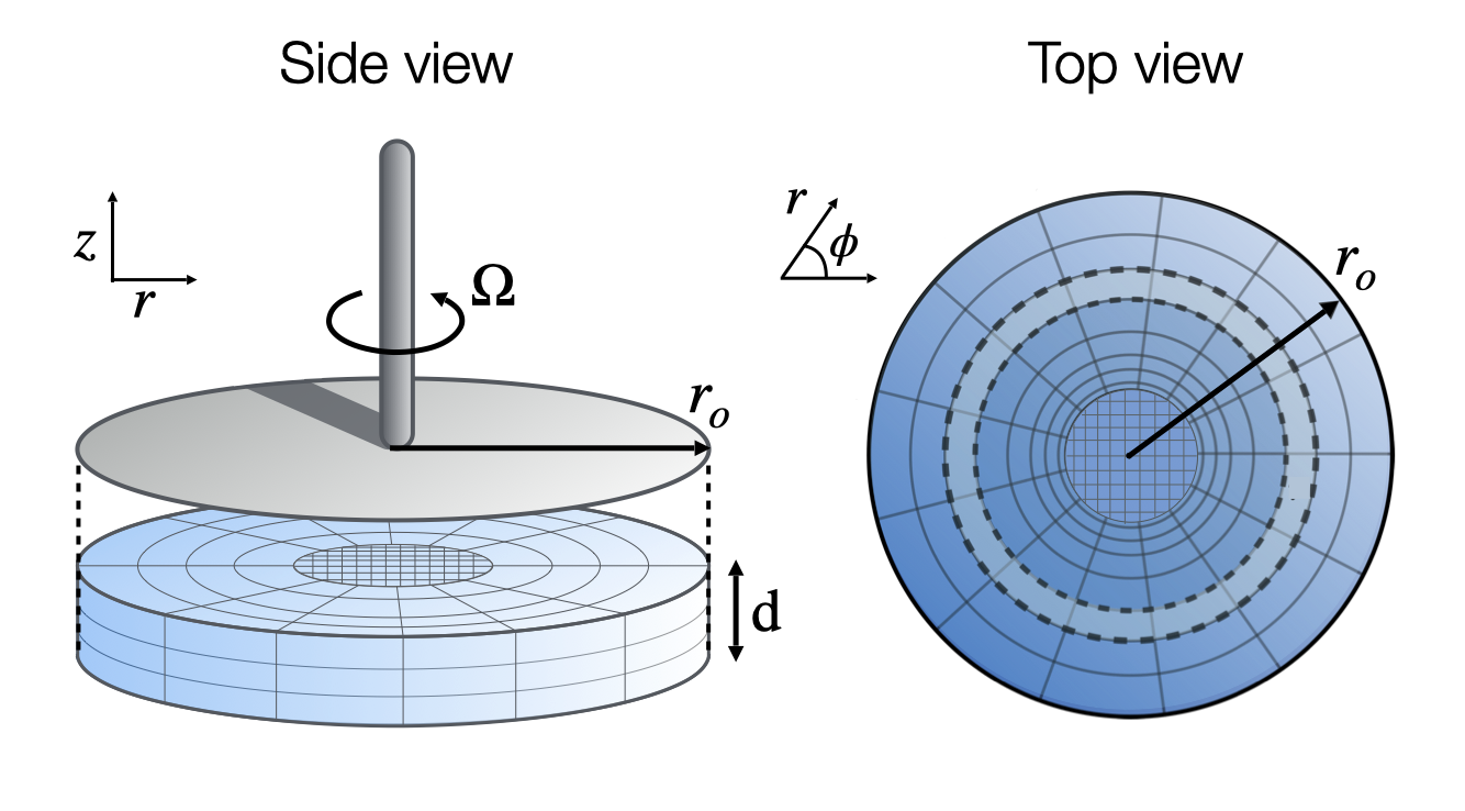
Figure 1: Schematic of the three-dimensional parallel plate geometry for simulating von Kármán swirling flow and the spokes-wheel mesh used in OpenFOAM^®   with $N_{r}=100$ cells in the radial direction, $N_{\phi}=120$ cells in the angular direction, and $N_{z}=10$ cells in the z-direction. Note, $30\times 30$ cells are distributed on a square lattice in the inner cylinder block. $\Omega$ is the angular velocity of the top plate with radius $r_{o}$, the bottom plate is fixed, and $d$ is the distance between the plates. For the angular average along the azimuthal angle $\phi$, we take the field values of cells with a fixed radius. An example is illustrated by the lighter shaded area surrounded by dashed lines. For the radial average along the radial direction, each contribution from a cell is weighted by the volume of the specific cell.

We consider an incompressible viscoelastic fluid in the geometry of a three-dimensional von Kármán swirling flow, where the viscoelastic fluid is constrained between two parallel plates with radius $r_{o}$ and the upper plate is rotating with angular velocity $\Omega$. A schematic of our set-up can be seen in Fig. 1. We use the characteristic length $r_{o}$ and the characteristic velocity $r_{o}\Omega$ to define the Reynolds number $\mathrm{Re}=\rho\Omega r_{o}^{2}/\eta_{s}$, where $\eta_{s}$ is the solvent shear viscosity. In the following, we set the Reynolds number $\mathrm{Re}\ll 1$, since we are interested in viscoelastic fluid flow at small scales, such as in microfluidic settings. In the following we always use the period of the plate rotation, $2\pi/\Omega$, to rescale time and frequency.

We calculate the dynamics of the flow field $\bm{u}(\bm{r},t)$, where $\bm{r}$ denotes the position and $t$ the time, using the generalized Navier-Stokes equation for an incompressible Oldroyd-B fluid. Neglecting the nonlinear inertial term to speed up the calculations, we have

$$\nabla\cdot\bm{u} =0\,,$$ (1)

$$\rho\frac{\partial\bm{u}}{\partial t} =-\nabla p+\eta_{s}\nabla^{2}\bm{u}+{\nabla\bm{\tau}}\,.$$ (2)

Here, $\rho$ is the density of the solvent, $p$ is the pressure, $\eta_{s}$ the solvent shear viscosity, and ${\nabla\bm{\tau}}$ denotes the divergence of the stress tensor $\bm{\tau}$. It describes the viscoelastic stresses, for example, due to dissolved polymers in polymer solutions. Concretely, we choose the constitutive relation of the Oldroyd-B model Oldroyd (1958, 1950) to model the viscoelastic stresses, which reads

$$\bm{\tau}+\lambda\overset{\nabla}{\bm{\tau}}=\eta_{p}\left(\bm{L}+\bm{L}^{\mathrm{T}}\right)\,.$$ (3)

Here, $\bm{L}=\nabla\otimes\bm{u}$ is the velocity gradient tensor, $\eta_{p}$ is the polymeric shear viscosity and $\lambda$ a characteristic relaxation time of the dissolved polymers. Lastly, $\overset{\nabla}{\bm{\tau}}$ denotes the upper convective derivative of the stress tensor defined as

$$\overset{\nabla}{\bm{\tau}}=\frac{\partial\bm{\tau}}{\partial t}+\bm{u}\cdot\nabla\bm{\tau}-\bm{L}\bm{\tau}-\bm{\tau}\bm{L}^{\mathrm{T}}\,.$$ (4)

The governing equations (1)-(3) can be written in dimensionless form with three relevant parameters. Besides the Reynolds number $\mathrm{Re}$, one has the ratio $\beta=\eta_{p}/\eta_{s}$ of the polymeric shear viscosity to the solvent shear viscosity and the Weissenberg number $\mathrm{Wi}=\lambda\dot{\gamma}$, where $\dot{\gamma}$ is the characteristic shear rate. For the parallel plate geometry the characteristic shear rate is the ratio of the angular velocity of the rotating plate to the gap width, $\dot{\gamma}=\Omega{r_{o}}/{d}$, and we have $\mathrm{Wi}=\lambda\Omega{r_{o}}/{d}$.

II.1 Computational method

Following our previous work van Buel, Schaaf, and Stark (2018), Eqs. (1)-(3) are solved using the open-source program OpenFOAM^® Weller et al. (1998), which is a finite-volume solver for computational fluid dynamics simulations on polyhedral grids. We adopt a specialized solver for viscoelastic fluids called rheoTool Favero et al. (2010), which is implemented in OpenFOAM^®. The rheoTool solver has been tested for accuracy in benchmark flows and it has been shown to have second-order accuracy in space and time Pimenta and Alves (2017).

Numerical evaluations of viscoelastic fluid flow can be unstable when the conformation tensor loses its positive definiteness due to numerical discretization errors. Regions near stagnation points or regions with strong deformation rates are sensitive to numerical instabilities and the effect is especially significant at high Weissenberg numbers Fattal and Kupferman (2005). Stability of the numerical flow field can be increased by introducing the log-conformation tensor approach Fattal and Kupferman (2004), which is based on taking the logarithm of the conformation tensor and which is implemented in the rheoTool solver. The positive definite conformation tensor $\bm{\mathrm{C}}$ is related to the polymeric stress tensor by

$$\bm{\tau}=\frac{\eta_{p}}{\lambda}\left(\bm{\mathrm{C}}-\bm{\mathrm{I}}\right)\,,$$ (5)

where $\bm{\mathrm{I}}$ is the identity tensor. Now, setting $\bm{\mathrm{\Theta}}=\ln\bm{\mathrm{C}}$, the constitutive relation (3) is transformed to a dynamic equation for $\bm{\mathrm{\Theta}}$, which is then numerically evaluated. More details of the method are given in Ref. Fattal and Kupferman, 2004. Evolving $\bm{\mathrm{\Theta}}$ in time and then transforming back to the conformation tensor $\bm{\mathrm{C}}$ and stress tensor $\bm{\tau}$ gives enhanced stability Pimenta and Alves (2017). However, the error in the conformation tensor $\bm{\mathrm{C}}$ increases, which is mitigated by setting a small time step in the numerical evaluation and by using a mesh refinement towards the inner cylinder, where discretization errors of the employed mesh increase. In our numerical calculations we further use a biconjugate gradient solver combined with a diagonal incomplete LU preconditioner (DILUP-BiCG) to solve for the components of the polymeric stress tensor and a conjugate gradient solver coupled to a diagonal incomplete Cholesky preconditioner (DIC-PCG) to solve for the velocity and pressure fields. They are available in OpenFOAM^® following the work of Ref. Pimenta and Alves, 2017.

In the schematic of the parallel plate geometry in Fig. 1 two types of lattices can be seen, a radial and a square lattice. The square lattice is implemented to remove the radial singularity in the middle of the cylinder. It consists of $\left(N_{\phi}/4\right)^{2}$ cells and is connected to the radial lattice at $r=0.1\,r_{o}$. At the inner radius of the radial lattice we choose a finer radial mesh compared to the outer cylinder such that the radial width $\Delta r$ of the grid cells is ${2.0}\mathrm{\cdot 10^{-3}}\,r_{o}$ at $0.1\,r_{o}$ and increases to $1.9\cdot 10^{-2}\,r_{o}$ at $r_{o}$.

At the lower and upper bounding plates we choose the no-slip boundary condition for the velocity field, a zero gradient for the pressure field, and extrapolate the gradient for the polymeric stress field to zero. Hence, the velocity at the lower plate is $\bm{u}=\bm{0}$ and at the upper plate $\bm{u}=r\Omega\bm{e}_{\phi}$. Importantly, at the sides of the cylindrical cell we set the normal component of the velocity field to zero ($u_{r}=0$) and apply the same boundary conditions for pressure and polymeric stress field as before. The simulations start with the viscoelastic fluid at rest, where pressure, flow, and stress fields are uniformly zero.

The following geometric parameters are chosen from the viewpoint of a microfluidic setting such that the Reynolds number is low. As required by OpenFOAM^®, we give all parameters in Si units. The outer radius of the geometry is set to $r_{o}=10^{-5}\,\mathrm{m}$, the height to $d=0.1\,r_{o}$, and the rotational velocity is $\Omega=0.38\,\mathrm{s^{-1}}$. We adjust the Weissenberg number by varying the polymeric relaxation time $\lambda\,\in[0,{\color[rgb]{0,0,0}9.9\,\mathrm{s}}]$. We set the polymeric shear viscosity to $\eta_{p}=0.0015\,{\mathrm{kg/ms}}$, the solvent shear viscosity to $\eta_{s}=0.001\,{\mathrm{kg/ms}}$, and the density to $\rho=1000\,\mathrm{kg/m^{3}}$. The ratio of the polymeric to the solvent viscosity is then $\beta={\eta_{p}}/{\eta_{s}}=3/2$. For the Reynolds number we obtain $\mathrm{Re}=\rho\Omega r_{o}^{2}/\eta_{s}=0.038$. We note to obtain a small Re in experiments large polymeric and solvent viscosities are commonly employed. Having in mind microfluidic settings, in our work we choose a small characteristic length, which is equivalent to studying polymeric fluids at larger spatial dimensions with a larger solvent and polymeric viscosity. The fluid flow is simulated up to ${800}\,\mathrm{s}$ (about $50$ to $235\lambda$) with a time step $\delta t=10^{-5}\,\mathrm{s}$ ($10^{-5}$ to $10^{-6}\lambda$). We extract the velocity, pressure, and stress fields every 5000 time steps (about $0.005$ to $0.02\lambda$). The time step and extraction interval are very small compared to the relaxation time.

II.2 Linear stability analysis

To investigate the stability of the von Kármán swirling flow of the Oldroyd-B fluid, we perform a linear stability analysis following the works of Refs.  Avgousti and Beris, 1993 and Öztekin and Brown, 1993. A perturbation is superimposed on the base flow solution for which we choose a product ansatz in the three cylindrical coordinates $r$, $\phi$, and $z$. Concretely, following Ref. Öztekin and Brown, 1993, we analyze the stability of the base flow ($\bm{\tau}^{0},\bm{u}^{0},p^{0}$) to radially localized small-amplitude disturbances of the form

$$\tilde{\bm{\tau}} =\bm{\tau}^{0}+\mathcal{R}\left[\bm{\tau}(z)\exp(i\alpha r+im\phi+\sigma t)\right]\,,$$ (6)

$$\tilde{\bm{u}} =\bm{u}^{0}+\mathcal{R}\left[\bm{u}(z)\exp(i\alpha r+im\phi+\sigma t)\right]\,,$$ (7)

$$\tilde{p} =p^{0}+\mathcal{R}\left[p(z)\exp(i\alpha r+im\phi+\sigma t)\right]\,,$$ (8)

where $\mathcal{R}[.]$ represents the real part, $\bm{\tau},\bm{u},p$ are small complex functions of the $z$ coordinate, $\alpha$ is the real-valued radial wave number, $m$ is the azimuthal wave number, and $\sigma$ is the complex frequency, which we determine from the eigenvalue problem. The azimuthal wave number $m$ is an integer, which can be positive or negative for non-axisymmetric disturbances, while $m=0$ corresponds to axisymmetric disturbances.

For the linear stability analysis we take the base flow solution of the governing equations (1)-(3) with the boundary condition

$$\bm{u}(r,\phi,0)=\bm{0}\enspace,\qquad\bm{u}(r,\phi,d)={r\Omega\bm{e}_{\phi}}\,,$$ (9)

where $\bm{e}_{\phi}$ is the unit vector in the azimuthal direction. Neglecting fluid inertia ($\text{Re}\approx 0$), the steady-state velocity field for infinitely extended parallel plates is purely azimuthal and given by

$$\bm{u}^{0}=\frac{r\Omega z}{d}\bm{e}_{\phi}\,.$$ (10)

The corresponding base stress and pressure fields read

$$\tau_{rr}^{0}=\tau_{r\phi}^{0}=\tau_{rz}^{0}=\tau_{zz}^{0}=0;\qquad\tau_{\phi z}^{0}=\eta_{p}\frac{r\Omega}{d};$$ (11)

$$\tau_{\phi\phi}^{0}=2\eta_{p}\lambda\left(\frac{r\Omega}{d}\right)^{2};\qquad p^{0}=-\eta_{p}\lambda\left(\frac{r\Omega}{d}\right)^{2}\,.$$ (12)

After substituting Eqs. (6)-(8) in the governing equations (1)-(3), using the fact that the base flow solves these equations, and disregarding all terms that are nonlinear in the disturbance amplitude, we obtain a set of 10 linear differential equations (see Appendix C). One can show that the linear stability analysis can be reduced to an ODE system of the form $\bm{\psi}^{\prime}=F(z,\bm{\psi})$ with 6 independent variables, which we express with the vector

$$\bm{\psi}=[u_{r}(z),u_{\phi}(z),p(z),u_{r}^{\prime}(z),u_{\phi}^{\prime}(z),p^{\prime}(z)]^{\mathrm{T}}\,,$$ (13)

where the prime indicates the derivative $g^{\prime}=dg/dz$ with respect to the spatial coordinate $z$. The remaining variables, such as the components of the polymeric stress tensor, are then obtained from the independent variables.

The boundary conditions of the velocity perturbation are set to

$$\bm{u}(r,\phi,z)={\bm{0}}\qquad\text{at $z=0$ and $z=1$}\,.$$ (14)

Moreover, we take the radially localized perturbation to occur at the edge of the rotating cylinder, $r=r_{o}$, where the shear rate is the highest and where we expect the perturbation to be strongest. Following Ref. Öztekin and Brown, 1993 this also means that in the set of linear equations we replace $r$ by $r_{o}$. We numerically solve the linear stability problem and identify the eigenvalue $\sigma$ in an iterative manner using a collocation method, which discretizes the perturbation functions in the $z$ direction, with the computer algorithm solve_bvp available in the SciPy package Virtanen et al. (2020).

We have validated our numerical algorithm against the results of Ref. Öztekin and Brown, 1993 and find good agreement with our findings as we demonstrate in Appendix C. The validation is essential given the large number of terms involved in the calculations. In section III.1 we perform the linear-stability analysis for our parameter setting.

III Results

In this section we describe our results. First, we analyze the stability of the base flow through linear stability analysis. Second, we display the initial evolution of an non-axisymmetric instability observed in our simulations before turbulent flow fully sets in. Then, we characterize the flow state above the critical Weissenberg number, where we observe turbulent and weakly chaotic flow. We further characterize both flow states through the flow resistance, the amount of work performed on the fluid surface. Finally, we analyze spatial and temporal power spectra of the velocity and stress fields.

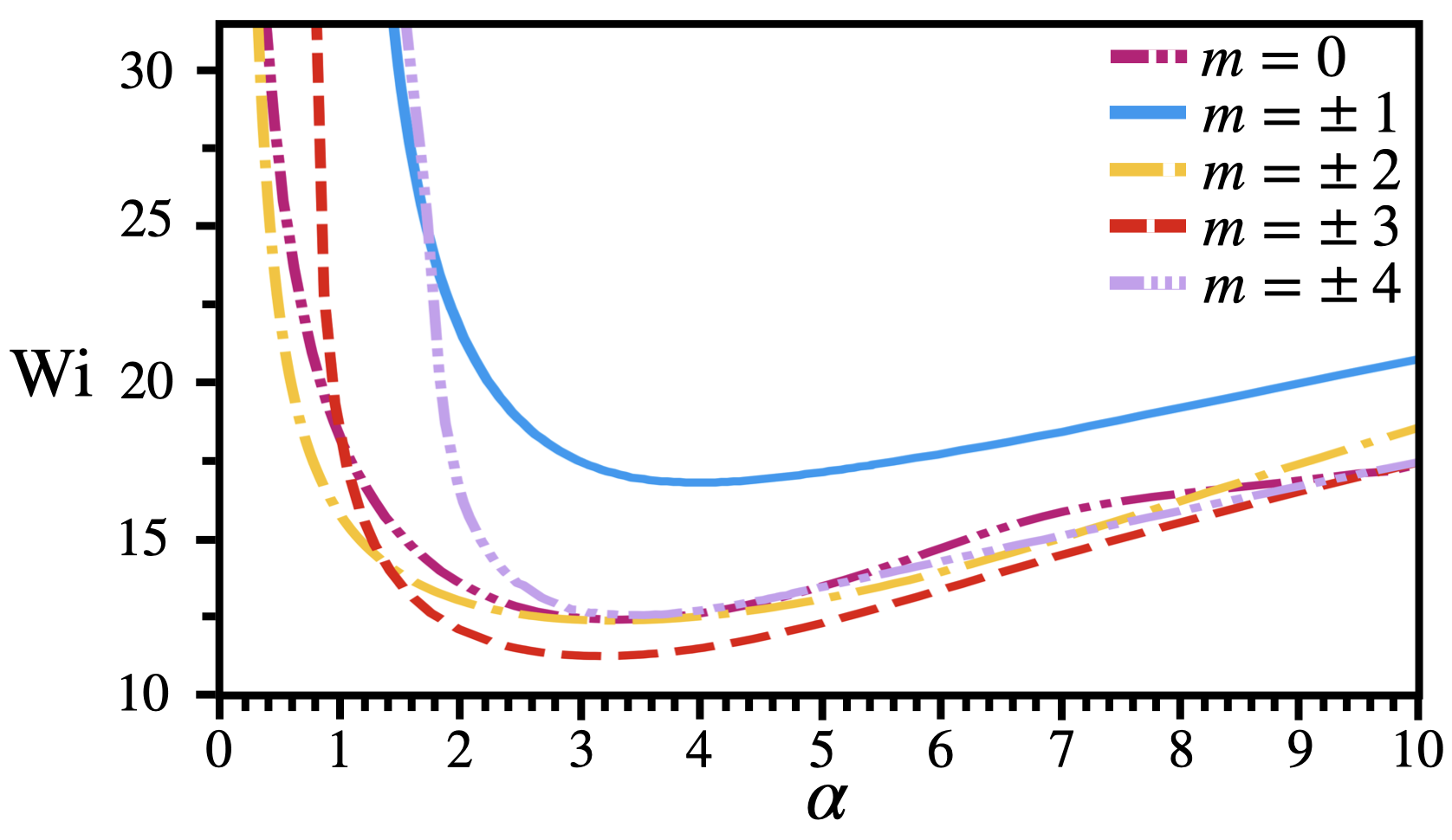
Figure 2: Neutral stability curves for the Oldroyd-B fluid in a von Kármán swirling flow in the plane Weissenberg number $\mathrm{Wi}$ versus radial wave number $\alpha$ for the first nine azimuthal modes ($-4\leq m\leq 4$). The stability curves of the different modes are indicated in the legend. The polymer to solvent viscosity ratio is set to $\beta=3/2$ and the critical radius to $r_{o}=10\,d$.

Table 1: The axisymmetric ($m=0$) and non-axisymmetric ($|m|=1,2,3$) modes become unstable at the critical Weissenberg number $\mathrm{Wi_{c}^{LSA}}$. Their critical axial wave number $\alpha_{c}$ and the oscillation frequency $\sigma_{\mathrm{im}}$ from the imaginary part of $\sigma$ are indicated. The polymer to solvent viscosity ratio is set to $\beta=3/2$ and the critical radius is $r_{c}=r_{o}=10\,d$.

$|m|$	0	1	2	3	4
$\mathrm{Wi_{c}^{LSA}}$	12.42	17.00	12.389	11.255	12.574
$\alpha_{c}$	3.30	3.50	3.30	3.25	3.50
$\sigma_{\mathrm{im}}$	-1.25	-1.25	-0.375	-0.345	-0.345

III.1 Linear stability analysis

First, we investigate the stability of the von Kármán base flow (see Fig. 1) using the methodology outlined in section II.2. We set the ratio of polymer to solvent viscosity to $\beta=3/2$ and the critical radius to $r_{o}=10\,d$. The critical conditions of the linear stability equations for axisymmetric and non-axisymmetric instabilities depend on the Weissenberg number $\mathrm{Wi}$ and on the radial wave number $\alpha$, which is a function of $\mathrm{Wi}$. Hence, for each wave number the Weissenberg number where the first eigenmode becomes unstable (real part of eigenvalue $\sigma_{\mathrm{re}}>0$) is determined. The neutral stability curves ($\sigma_{\mathrm{re}}=0$) separating stable from unstable regions for the axisymmetric ($m=0$) and non-axisymmetric ($0<|m|\leq 4$) modes are presented in the $\alpha$-$\mathrm{Wi}$ plane in Fig. 2. The critical wave number $\alpha_{c}$ for each $m$ is then obtained from the absolute minimum of each curve. However, the minima of all the curves are shallow and excluding $m=\pm 1$ they are close to each other, implying that bands of axial wave numbers become unstable when the Weissenberg number is slightly increased above the critical value $\mathrm{Wi}_{c}$. The results of the most unstable axisymmetric and non-axisymmetric modes are presented in Table 1.

First of all, we find that the von Kármán base flow becomes linearly unstable, which first happens for non-axisymmetric disturbances with azimuthal wave numbers $m=\pm 3$. The instability occurs at the critical radial wave number $\alpha_{c}=3.25$ and critical Weissenberg number $\mathrm{Wi_{c}^{LSA}}=11.255$, where the superscript refers to the result of the linear stability analysis. Moreover, the neutral stability curves for the axisymmetric mode and two non-axisymmetric modes ($|m|=2,4$) are very close to each other around the minima. This demonstrates that multiple modes become unstable when the Weissenberg number is slightly increased above the critical value of the $|m|=2$ modes. We note that shallow minima are also observed in the neutral stability curves of Taylor-Couette flow at low Reynolds numbers in Ref. Avgousti and Beris, 1993.

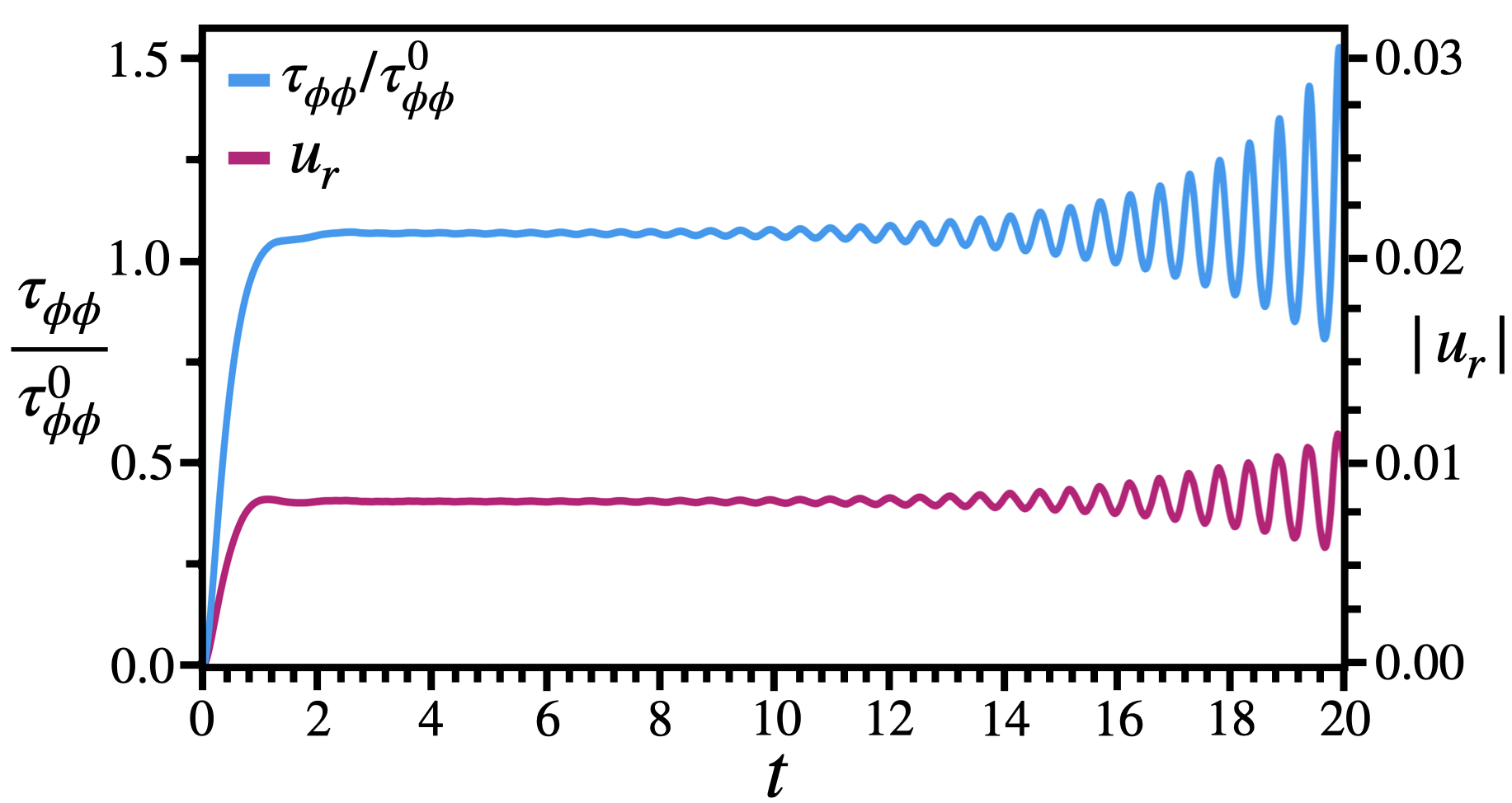
Figure 3: Azimuthal component of the stress tensor $\tau_{\phi\phi}$ normalized by the base flow $\tau_{\phi\phi}^{0}$ (left axis) and the magnitude of the radial velocity component $|u_{r}|$ (right axis) plotted versus time $t$ at $\mathrm{Wi}=12.008$ The components are recorded at position $(r,\phi,z)=(0.99\,r_{o},0,d/2)$.

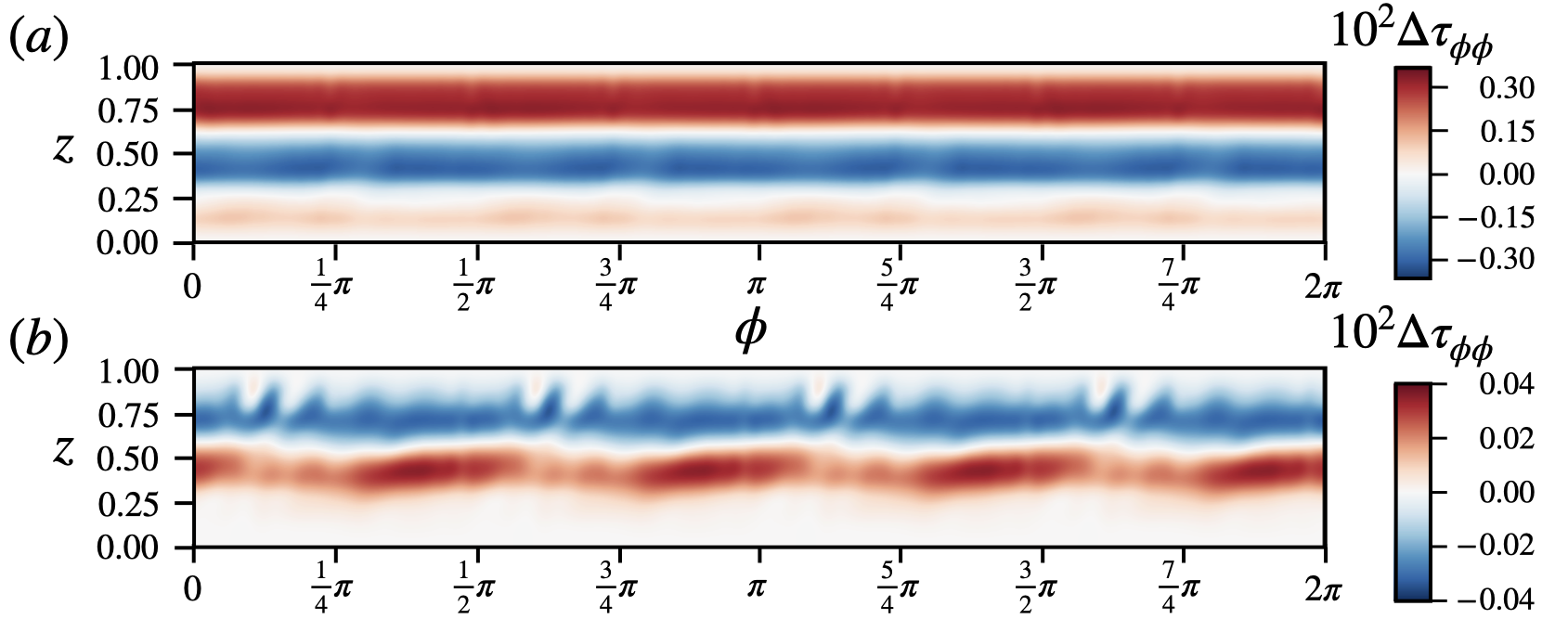
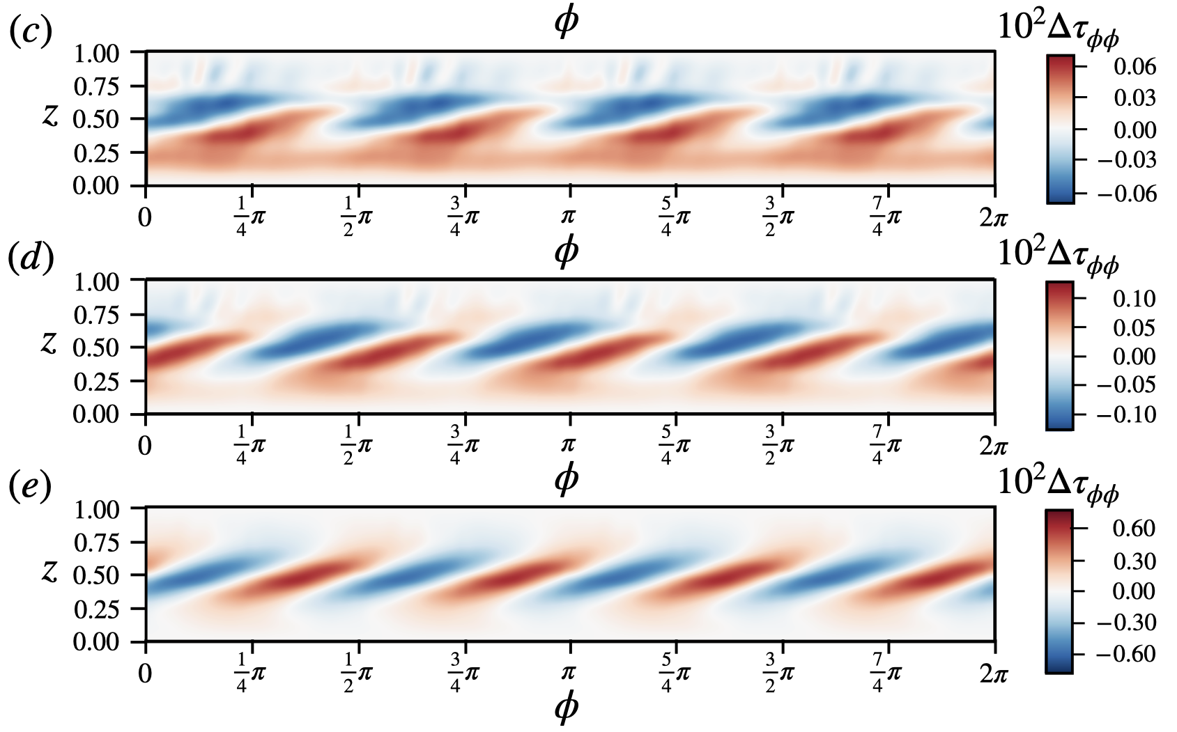
Figure 4: (Multimedia view) Azimuthal stress-tensor component color-coded in the $z-\phi$ plane near the outer radius $r=0.99\,r_{o}$ at $\mathrm{Wi}=12.008$. The component $\Delta\tau_{\phi\phi}=\tau_{\phi\phi}-\overline{\tau_{\phi\phi}}|_{t_{s}}^{t_{e}}$ is given relative to the mean value between times $t_{s}=2$ and $t_{e}=3$. Snapshots of the stress field are taken at times: (a) $t=1.4$, (b) $t=2.5$, (c) $t=7.6$, (d) $t=10.0$ and (e) $t=15.0$.

III.2 Onset of the instability

Now, we investigate the onset of the flow instability occurring in the simulations of the Oldroyd-B fluid of the von Kármán swirling flow. In contrast to the results from section III.1, we find a critical Weissenberg number around $\mathrm{Wi_{c}}\approx 12$ and observe, before the turbulent flow fully develops, an unstable non-axisymmetric mode with azimuthal wave numbers $m=\pm 4$, which we describe below.

All simulations start with the fluid at rest. During the initial state an axisymmetric disturbance flow occurs, which begins at the outer edge and then travels inwards, see for example Fig. 19. For low Weissenberg numbers $\mathrm{Wi}<\mathrm{Wi_{c}}$ it develops into a stable laminar flow. However, at $\mathrm{Wi}=12.008$ slightly above the critical value from our linear stability analysis, $\mathrm{Wi_{c}^{LSA}}=11.255$, we observe an unstable periodic disturbance flow. The temporal evolution of the disturbance is illustrated in Fig. 3, where we plot the azimuthal component of the stress tensor $\tau_{\phi\phi}$ normalized by the base flow value $\tau_{\phi\phi}^{0}$ and the radial component of the velocity field $|u_{r}|$ at position $(r,\phi,z)=(0.99\,r_{o},0,d/2)$. Both quantities oscillate with frequency $f=0.522$ and grow exponentially. Similar behavior occurs at $\mathrm{Wi}=12.16$ and $\mathrm{Wi}=12.92$. Thus, above $\mathrm{Wi}>12$ we observe a single unstable mode, which ultimately develops into a chaotic flow state.

Furthermore, we display the spatial and temporal appearance of the flow instability in Fig. 4 (Multimedia view), where we show the color-coded stress component $\tau_{\phi\phi}$ in the $z-\phi$ plane near the outer cylinder ($r=0.99\,r_{o}$) in time and present snapshots at several instances. First, Fig. 4 (a) shows the axisymmetric stress pattern, which has a positive stress value at the upper and lower plate and a negative value in between. The disturbance travels radially inward. At later time, in Fig. 4 (b) the line of zero stress close to the midplane between the two plates ($z=d/2$) becomes sinusoidal. Thus, a non-axisymmetric mode with four-fold symmetry develops. Its amplitude grows further in time and the zero-stress line strongly deviates from the sinusoidal shape [see Fig. 4 (c)]. Ultimately, tilted regions of positive and negative azimuthal stress appear along nearly the entire height of the von Kármán geometry. They alternate in the azimuthal direction, as Figs. 4(d) and (e) show. The amplitude of the pattern grows steadily in time and the whole pattern starts to slowly rotate about the vertical in the direction of the base flow until a chaotic flow pattern emerges. The development of the instability is reminiscent of a Kelvin-Helmholtz instability observed in sheared Newtonian fluids Chandrasekhar (2013).

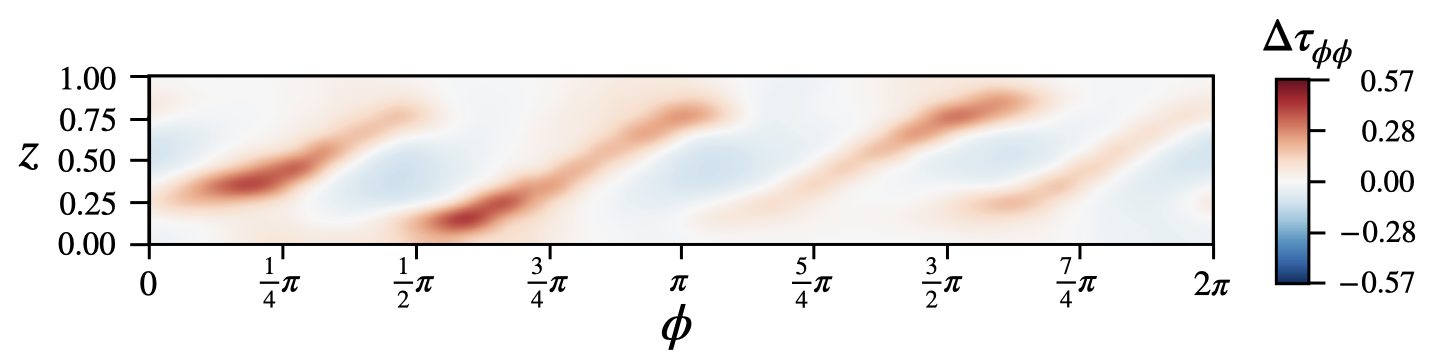
Figure 5: (Multimedia view) Azimuthal stress-tensor component color-coded in the $z-\phi$ plane near the outer radius $r=0.99\,r_{o}$ at $\mathrm{Wi}=12.16$. The component $\Delta\tau_{\phi\phi}=\tau_{\phi\phi}-\overline{\tau_{\phi\phi}}|_{t_{s}}^{t_{e}}$ is given relative to the mean value between times $t_{s}=2$ and $t_{e}=10$. Snapshot of the stress field is taken at time $t=21.54$ and it displays weakly chaotic flow (see Sec. III.3). The video shows the transition from the laminar flow to the weakly chaotic flow and ultimately elastic turbulence.

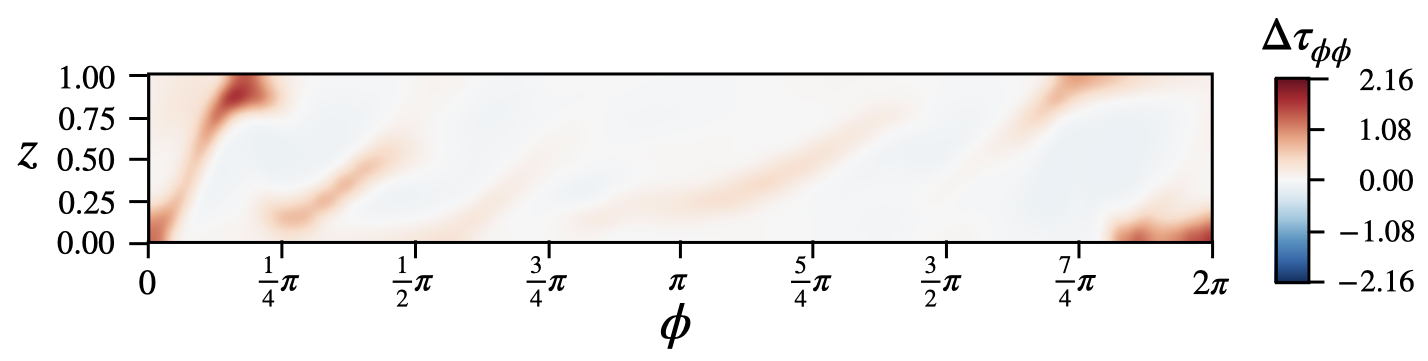
Figure 6: (Multimedia view) Azimuthal stress-tensor component color-coded in the $z-\phi$ plane near the outer radius $r=0.99\,r_{o}$ at $\mathrm{Wi}=12.92$. The component $\Delta\tau_{\phi\phi}=\tau_{\phi\phi}-\overline{\tau_{\phi\phi}}|_{t_{s}}^{t_{e}}$ is given relative to the mean value between times $t_{s}=2$ and $t_{e}=3$. Snapshot of the stress field is taken at time $t=19.63$ and it displays elastic turbulence (see Sec. III.3). The video shows the transition from the laminar flow to the weakly chaotic flow and ultimately elastic turbulence.

Likewise, we observe similar spatiotemporal behavior at $\mathrm{Wi}=12.16$ and $\mathrm{Wi}=12.92$. We present videos of the color-coded stress component $\tau_{\phi\phi}$ in the $z-\phi$ plane near the outer cylinder ($r=0.99\,r_{o}$) as a function of time in Fig. 5 (Multimedia view) for $\mathrm{Wi}=12.16$ and in Fig. 6 (Multimedia view) for $\mathrm{Wi}=12.92$. The videos show the same development of the instability as the one above. An unstable nonaxisymmetric mode with four-fold symmetry drives the laminar flow towards an weakly chaotic flow and ultimately to a chaotic flow, which we characterize as turbulent in the next section. The snapshot presented in Fig. 5 represents weakly chaotic flow, while the snapshot presented in Fig. 6 represents elastic turbulence. Both flow states are discussed in detail in the next section.

The obvious difference between the linear stability analysis, which predicts the $|m|=3$ modes as the most unstable modes, and the result of the numerical simulations can be due to simplifications used in the linear stability analysis. In the ansatz functions (6) to (8) the spatial dependence on $z$ and $r$ is decoupled and an infinitesimal flow field is assumed, whereas in the numerical solutions a more general variation in $z$, $r$ is allowed. Additionally, the von Kármán geometry has a finite extension with an additional boundary condition for the flow field at the outer cylindrical boundary ($u_{r}=0$ at $r=r_{o}$). Moreover, the spatial discretization used in the simulations is constructed with four-fold symmetry (starting from four connected trapezoidal prisms) leading to small numerical errors, which reflect this symmetry. This could result in lowering the critical conditions for the $|m|=4$ mode. To analyze the influence of the mesh symmetry, we performed additional simulations with a spatial discretization with three-fold symmetry (starting from three connected trapezoidal prisms). These simulations at $\mathrm{Wi}=11.78$, $\mathrm{Wi}=12.16$ and $\mathrm{Wi}=12.92$ all show a non-axisymmetric pattern with four-fold symmetry developing from the base flow. Therefore, we conclude that the observed difference in the most unstable mode is not due to the symmetry of the mesh discretization.

III.3 Characterizing elastic turbulence

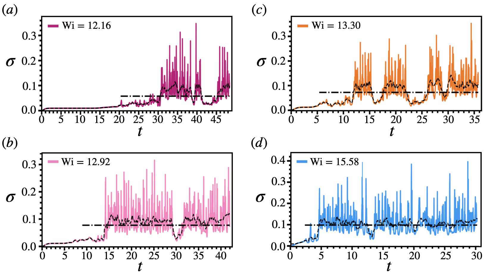
Figure 7: Secondary-flow strength $\sigma$ defined in Eq. (15) plotted as a function of time $t$ in units of $2\pi/\Omega$. The Weissenberg number is (a) $\mathrm{Wi}=12.16$, (b) $\mathrm{Wi}=12.92$, (c) $\mathrm{Wi}=13.3$, and (d) $\mathrm{Wi}=15.58$. The temporal average of the secondary-flow strength, $\overline{\sigma}(t>t_{0})$, is displayed with the black dash-dotted line and starts at $t_{0}$, which is the first time with $\sigma\geq 0.025$. The moving average, $\sigma_{\delta}(t)=\frac{1}{2\delta}\int_{t-\delta t}^{t+\delta t}\sigma(t^{\prime})dt^{\prime}$ with $\delta t=0.3$, is indicated by the black dashed line. Two distinct flow states are distinguished: a turbulent state where $\sigma(t)$ strongly fluctuates around $\langle\sigma\rangle\approx 0.1$ and an weakly chaotic time-dependent state with only small fluctuations of $\sigma(t)$ around a significantly smaller mean value. The state of the fluid flow can be identified as turbulent ($\sigma_{\delta}>\overline{\sigma}$), as weakly chaotic ($\sigma_{\delta}<\overline{\sigma}$), or as laminar ($\sigma\approx 0$).

Here we demonstrate the occurrence of an elastic instability which ultimately develops into elastic turbulence. The onset of the elastic instability is indicated by the critical Weissenberg number $\mathrm{Wi_{c}}$. To investigate and characterize the transition, we define an order parameter $\Phi=\overline{\sigma(t)}$, as the time average of the normalized velocity fluctuations

$$\sigma(t)\equiv\left.\sqrt{\left\langle\left[\bm{u}(\bm{r},t)-{\bm{u}^{0}(\bm{r})}\right]^{2}\right\rangle}\right/u^{0}_{\mathrm{max}}\,,$$ (15)

relative to the base flow field $\bm{u}^{0}(\bm{r})$, for which we choose the numerical solution at $\mathrm{Wi}=0$. It deviates from the flow field of Eq. (10) since the bounding parallel plates are not infinitely extended. Here $\langle\dots\rangle=\frac{1}{V}\int\dots dV$ denotes the volume average and $u^{0}_{\mathrm{max}}=\Omega r_{o}$ is the maximum velocity of the rotating upper plate, which is used to normalize $\sigma$. We call $\sigma(t)$ the secondary-flow strength. Our order parameter is similar to the turbulence kinetic energy $\epsilon$, the time-averaged kinetic energy of the velocity fluctuations, which reads

$$\epsilon=\frac{1}{2}\overline{\left\langle\left[\bm{u}(\bm{r},t)-\overline{\bm{u}(\bm{r},t)}\right]^{2}\right\rangle}\,.$$ (16)

However, both parameters scale differently; while $\epsilon\sim\bm{u}^{2}$, our order parameter $\Phi\sim\bm{u}$. It is a linear measure for the relative strength of the velocity fluctuations and we use it to quantify the deviation from the base flow when a secondary flow occurs.

III.3.1 Velocity fluctuations

In previous work we have shown an elastically driven instability in a two-dimensional Taylor-Couette flow, where the order parameter sharply increases beyond a critical Weissenberg number $\mathrm{Wi_{c}}$ van Buel, Schaaf, and Stark (2018). Now, we characterize this transition in the three-dimensional geometry of the von Kármán swirling flow. In Fig. 7 (a)-(d) we plot the secondary-flow strength $\sigma$ as a function of time $t$ for four different Weissenberg numbers in the range $12.16\leq\mathrm{Wi}\leq 15.58$ starting from a fluid at rest at $t=0$. From the figure it can be observed that both the fluctuations of the secondary-flow strength and its mean, indicated by the dash-dotted line, increase with increasing $\mathrm{Wi}$. Moreover, $\sigma(t)$ reveals bursts of strong velocity fluctuations interrupted by more quiescent flow. Thus, we distinguish two types of time-dependent flows: the first, which we denote weakly chaotic, comprises small fluctuations in $\sigma$ around a small mean value, while the second turbulent branch shows large fluctuations in $\sigma$ around a mean value $\langle\sigma\rangle\approx 0.1$.

For Weissenberg numbers in the range $12\leq\mathrm{Wi}<20$ the flow is bistable, it randomly switches between both flow states. Determining the time where steady-state is reached is difficult, since the mean value of $\sigma$ depends on how often the flow randomly switches between both states. Therefore, in this work we have the following convention: the time-dependent weakly chaotic flow with its small fluctuations starts when $\sigma$ exceeds the value 0.025, which is chosen by visual inspection. The time of the first occurrence of $\sigma\geq 0.025$ is denoted $t_{0}$ and here we start with the averaging of $\sigma$. An important observation in Fig. 7 is that the instability takes significantly longer to set in at Weissenberg numbers closer to $\mathrm{Wi}=12$, i.e., $t_{0}$ decreases with increasing $\mathrm{Wi}$. For example, at $\mathrm{Wi}=12.16$ it takes about 20 rotations (corresponding to $t_{0}\approx 100\lambda$), whereas at $\mathrm{Wi}=15.58$ it takes about 3 rotations (corresponding to $t_{0}\approx 12\lambda$).

III.3.2 Order parameter

To capture and describe the two different time-dependent flow states, we cannot simply look at the order parameter, $\Phi=\overline{\sigma}$, as the total time average over $\sigma$. Moreover, unless the total simulation time approaches infinity, $\Phi$ strongly depends on the time where averaging starts. Therefore, we need a more careful treatment. First, we properly define the mean secondary-flow strength, ${\sigma_{0}}=\overline{\sigma(t>t_{0})}$, by starting the average at $t_{0}$. In Fig. 7 it is indicated as the black dash-dotted line starting at $t=t_{0}$. Additionally, a moving average $\sigma_{\delta}$ is displayed in Fig. 7 by the black dashed line. The moving average is defined as $\sigma_{\delta}(t)=\frac{1}{2\delta}\int_{t-\delta t}^{t+\delta t}\sigma(t^{\prime})dt^{\prime}$, where we have set $\delta t=0.3$. At the start and end of the time series the integral is limited to the range of $\sigma(t)$. Thus, the normalization factor $(2\delta)^{-1}$ is adjusted to the range of the integral, accordingly. Now, we are able to introduce order parameters for the two flow states of the fluid by averaging only over time traces $\sigma(t)$, which belong to either the turbulent (II) or weakly chaotic (I) flow state:

$$\Phi=\begin{cases}\Phi^{\mathrm{II}}=\overline{\sigma(t)}&\enspace\text{with}\enspace\sigma_{\delta}(t)\geq{\sigma_{0}},\enspace t>t_{0},\\ \Phi^{\mathrm{I\,}}=\overline{\sigma(t)}&\enspace\text{with}\enspace\sigma_{\delta}(t)<{\sigma_{0}},\enspace t>t_{0}.\end{cases}$$ (17)

The order parameters are plotted in Fig. 8 as a function of the Weissenberg number. A clear transition from the laminar base flow where $\Phi\approx 0$ to the occurrence of two types of secondary-flows with $\Phi^{\mathrm{I}},\Phi^{\mathrm{II}}>0$ is observed upon increasing the elasticity of the fluid beyond a critical value of $\mathrm{Wi}_{c}=12$. Moreover, the order parameters for both flow types show a subcritical transition upon increasing the Weissenberg number beyond the critical value. A subcritical transition is also predicted in theory for the Oldroyd-B model by linear stability analysis Walsh (1987); Öztekin and Brown (1993) and observed in experiments Groisman and Steinberg (2004); Burghelea, Segre, and Steinberg (2007). Remarkably, our observed $\mathrm{Wi}_{c}$ is close to the critical value $\mathrm{Wi}=12.5$ observed in experiments with the same aspect ratio $d/r_{o}$ but at a higher polymer viscosity $\beta=0.8$ Burghelea, Segre, and Steinberg (2007).

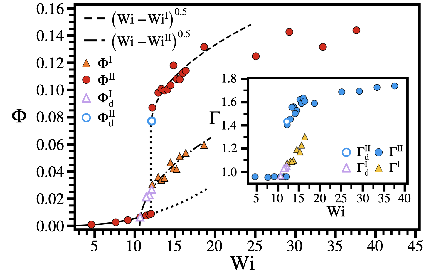
Figure 8: Order parameter $\Phi=\overline{\sigma}$ as a function of the Weissenberg number $\mathrm{Wi}=\Omega\lambda r_{o}/d$. Closed symbols indicate the order parameter as defined in Eq. (17) for simulations starting with a fluid at rest. The red circles denote the turbulent branch $\Phi^{\mathrm{II}}$ and the orange triangles denote the weakly chaotic branch $\Phi^{\mathrm{I}}$. Below the subcritical transition at $\mathrm{Wi_{c}}=12$ both branches merge and $\Phi^{\mathrm{I}}=\Phi^{\mathrm{II}}$. The dashed and dash-dotted lines show fits to square root scaling close to $\mathrm{Wi_{c}}$ using $\Phi^{\mathrm{I}}\sim\left({\mathrm{Wi}-\!\mathrm{Wi^{\mathrm{I}}}}\right)^{0.5}$ with $\mathrm{Wi}^{\mathrm{I}}=10.6$ and $\Phi^{\mathrm{II}}\sim\left({\mathrm{Wi}-\!\mathrm{Wi^{\mathrm{II}}}}\right)^{0.5}+\Phi_{0}$ with $\mathrm{Wi}^{\mathrm{II}}=12$ and $\Phi_{0}=0.073$, respectively. Dotted lines are given as guides to the eye. Open symbols indicate the order parameters $\Phi^{\mathrm{I}}_{\mathrm{d}}$ and $\Phi^{\mathrm{II}}_{\mathrm{d}}$ when the simulations run for 26 rotations at $\mathrm{Wi}=15.96$ and then $\mathrm{Wi}$ is dropped to its actual value. Hysteretic behavior is observed for the lower branch. Inset: Flow resistance $\Gamma$ for the turbulent (II) and weakly chaotic (I) branch.

III.3.3 Flow resistance

Another characteristic of elastic turbulence is a sharp increase in the flow resistance Groisman and Steinberg (2000, 2004); van Buel, Schaaf, and Stark (2018). We define the flow resistance using the total work performed on the fluid per unit time and unit volume,

$$W=\frac{1}{V}\oint\bm{u}\cdot\bm{T}\bm{n}\,dA\,,$$ (18)

where $\bm{T}=-p\bm{I}+\eta_{s}[\nabla\otimes\bm{v}+(\nabla\otimes\bm{v})^{\mathrm{T}}]+\bm{\tau}$ is the Cauchy stress tensor, $\bm{n}$ is the surface normal vector, $V$ is the volume, and we integrate over the total surface $A$ of the fluid. $W$ has both a viscous and elastic contribution, $W=W_{\mathrm{v}}+W_{\mathrm{el}}$. For an elastically driven instability we expect $W_{\mathrm{el}}>W_{\mathrm{v}}$, since we expect the elastic stresses to sharply increase after the transition compared to the velocity gradients in the flow. The elastic contribution to the total work results from the polymeric stress tensor and for the von Kármán swirling flow reads

$$W_{\mathrm{el}}=\frac{1}{V}\int u_{\phi}\tau_{z\phi}dA_{t}+\frac{1}{V}\int(u_{\phi}\tau_{r\phi}+u_{z}\tau_{rz})dA_{s}\,,$$ (19)

where $A_{t}$ is the area of the fluid at the upper plate ($\bm{n}=\bm{e}_{z}$) and $A_{s}$ is the area of the fluid at the side ($\bm{n}=\bm{e}_{r}$). Note that our boundary condition sets $u_{r}=0$ at the side and at the top plate $u_{\phi}=r\Omega$ is the only non-zero velocity component. Likewise, the viscous contribution from the solvent is given by

$$W_{\mathrm{v}}=\frac{2\eta_{s}}{V}\int u_{\phi}D_{z\phi}dA_{t}+\frac{2\eta_{s}}{V}\int(u_{\phi}D_{r\phi}+u_{z}D_{rz})dA_{s}\,,$$ (20)

where $\bm{D}=\frac{1}{2}[\nabla\otimes\bm{u}+(\nabla\otimes\bm{u})^{\mathrm{T}}]$ is the deformation rate tensor. For the laminar base flow, excluding edge effects, we have

$$W_{\mathrm{el}}^{0}=\frac{\eta_{p}}{2d}\left(\frac{\Omega r_{o}}{d}\right)^{2}\quad{\color[rgb]{0,0,0}\text{and}}\quad\enspace W_{\mathrm{v}}^{0}=\frac{\eta_{s}}{2d}\left(\frac{\Omega r_{o}}{d}\right)^{2}\,.$$ (21)

Now we define the flow resistance $\Gamma=\overline{W(t)}/W^{0}$, where the temporal mean work $\overline{W(t)}$ is normalized by the laminar-base-flow value $W^{0}$. Corresponding to the two time-dependent fluctuating flow states, we also introduce the flow resistances of the turbulent (II) and weakly chaotic (I) state:

$$\Gamma=\begin{cases}\Gamma^{\mathrm{II}}=\overline{W(t)}/W^{0}&\enspace\text{with}\enspace\sigma_{\delta}(t)\geq{\sigma_{0}},\!\enspace t>t_{0},\\ \Gamma^{\mathrm{I}}\;=\overline{W(t)}/W^{0}&\enspace\text{with}\enspace\sigma_{\delta}(t)<{\sigma_{0}},\!\enspace t>t_{0}.\end{cases}$$ (22)

We plot $\Gamma$ in the inset of Fig. 8. A clear and sudden increase in the flow resistance beyond the critical Weissenberg number can be observed, associated with the subcritical transition indicated be the order parameter. At the transition to the turbulent branch (filled blue circles above $\mathrm{Wi_{c}}$) the flow resistance jumps by $0.4\,\Gamma_{0}$, which is below the experimentally observed value Burghelea, Segre, and Steinberg (2007). For the weakly chaotic flow (filled yellow triangles) the jump is $0.1\,\Gamma_{0}$, four times less than the turbulent branch, and the normalized flow resistance goes up to 1.3. For $\mathrm{Wi}>18$ the weakly chaotic flow state is no longer observed and therefore only the turbulent branch remains. The total value of the flow resistance $\Gamma$ as a function of $\mathrm{Wi}$ is in the range $1<\Gamma<2$, which is about half of the values observed in experiments Burghelea, Segre, and Steinberg (2007). For $\mathrm{Wi}>18$ the flow resistance $\Gamma$ becomes nearly constant in our simulations. This might be due to discretization errors such that simulations at higher $\mathrm{Wi}$ require finer meshes. Accurately resolving this discrepancy is beyond our current capabilities.

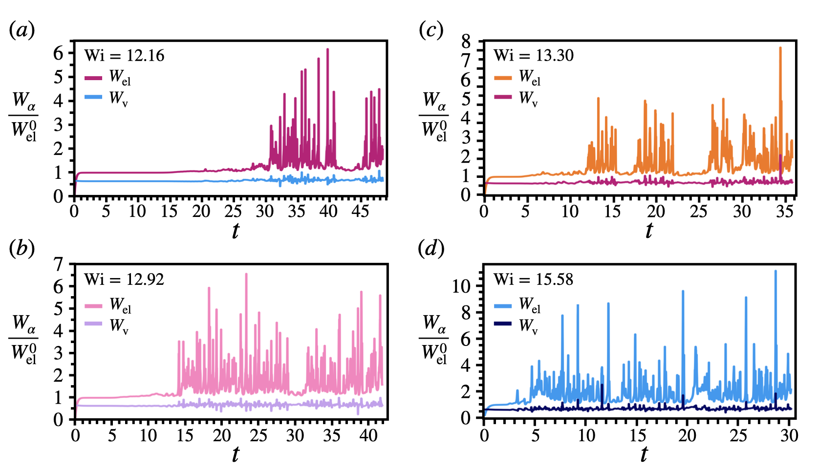
Figure 9: Work $W_{\alpha}$ performed on the viscoelastic fluid by the viscous stresses $W_{\mathrm{v}}$ and the elastic stresses $W_{\mathrm{el}}$ plotted versus time and normalized by the base flow value $W^{0}_{\mathrm{el}}$ [see Eqs. (21), left]. The index $\alpha$ refers to the elastic ($W_{\mathrm{el}}$) or viscous ($W_{\mathrm{v}}$) contribution, respectively. Data are shown for four values of the Weissenberg number with (a) $\mathrm{Wi}=12.16$, (b) $\mathrm{Wi}=12.92$, (c) $\mathrm{Wi}=13.30$ and (d) $\mathrm{Wi}=15.58$.

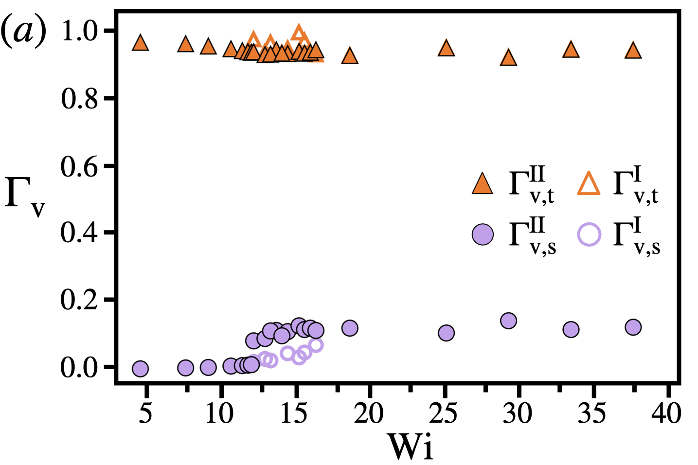
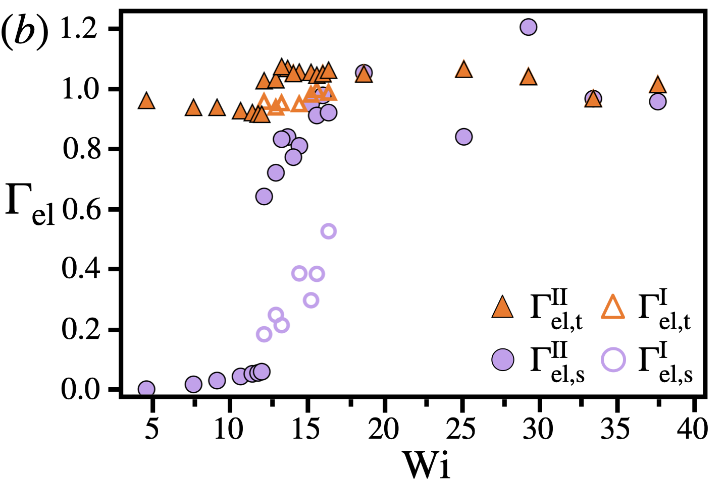
Figure 10: (a) Viscous part of the flow resistance $\Gamma_{\mathrm{v},\nu}^{\mathrm{I/II}}=\overline{W_{\mathrm{v},\nu}}/W_{\mathrm{v}}^{0}$ and (b) elastic part of the flow resistance $\Gamma_{\mathrm{el},\nu}^{\mathrm{I/II}}=\overline{W_{\mathrm{el},\nu}}/{\color[rgb]{0,0,0}W_{\mathrm{el}}^{0}}$ plotted versus $\mathrm{Wi}$. The subscripts $\nu=t,s$ refer to the top (orange triangles) and side surface (purple circles), respectively. The superscripts I, II refer to weakly chaotic (open symbols) and turbulent/laminar flow (closed symbols), respectively.

III.3.4 Elastic and viscous work

Next, we discuss the total work $W$ in more detail. We first analyze the viscous ($W_{\mathrm{v}}$) and elastic ($W_{\mathrm{el}}$) parts relative to the base flow values and then evaluate the contributions from the two surfaces $A_{t}$ and $A_{s}$.

The normalized viscous and elastic contributions to the total work per unit time, $W_{\mathrm{v}}/W_{\mathrm{el}}^{0}$ and $W_{\mathrm{el}}/W_{\mathrm{el}}^{0}$, are plotted versus time in Fig. 9 for different $\mathrm{Wi}$. As reference we have chosen the base flow value $W_{\mathrm{el}}^{0}$ from Eq. (21), which is related to the viscous base flow value $W_{\mathrm{v}}^{0}$ by $W_{\mathrm{el}}^{0}=\beta\,W_{\mathrm{v}}^{0}$. At $\mathrm{Wi}=12.16$ [plot (a)], just above the critical Weissenberg number, we only observe slight fluctuations in the weakly chaotic state, whereas large fluctuations are present in the turbulent state. This is in full analogy to the secondary flow strength, presented in Fig. 7. The fluctuations in the turbulent state of both the viscous and the elastic stresses increase in magnitude for higher $\mathrm{Wi}$. Before the onset of the elastic instability, in the laminar flow state, the viscous work $W_{\mathrm{v}}/W^{0}_{\mathrm{el}}=1/\beta=2/3$ and the elastic work $W_{\mathrm{el}}/W^{0}_{\mathrm{el}}=1$ are equal to their respective base flow values. Generally, the magnitude of the fluctuations in $W_{\mathrm{v}}$ are small compared to the fluctuations in $W_{\mathrm{el}}$. The time-averaged value of $W_{\mathrm{v}}$ remains close to $\beta^{-1}$, i.e., $\overline{W_{\mathrm{v}}}/W_{\mathrm{v}}^{0}\approx 1$, while the average value of $W_{\mathrm{el}}$ increases. Thus, $W_{\mathrm{el}}>W_{\mathrm{v}}$ as one expects for an elastically driven instability and as it is also demonstrated by Fig. 9. Therefore, we conclude that the increase in the flow resistance $\Gamma$, the normalized total work per unit time, is mainly due to the elastic work performed on the fluid.

Next, we discuss the contributions from the different surface areas of the cylindrical geometry to the flow resistance. We distinguish between the viscous and elastic contributions of the work performed on the top and the side surface areas. We do not need to consider the bottom area since the work is always zero ($\bm{u}=0$). The two unsteady flow states, turbulent (II) and weakly chaotic (I), combined with the two surface areas give four specific contributions to the flow resistance, which we describe by

$$\Gamma_{\alpha,\nu}=\begin{cases}\Gamma^{\mathrm{II}}_{\alpha,\nu}=\overline{W_{\alpha,\nu}(t)}/W_{\alpha}^{0}\enspace\enspace\text{with}\enspace\sigma_{\delta}(t)\geq{\sigma_{0}},\enspace t>t_{0},\\ \Gamma^{\mathrm{I}}_{\alpha,\nu}=\overline{W_{\alpha,\nu}(t)}/W_{\alpha}^{0}\enspace\enspace\text{with}\enspace\sigma_{\delta}(t)<{\sigma_{0}},\enspace t>t_{0},\end{cases}$$ (23)

where in the following, we will use the superscript II also for the laminar state. Here, $\alpha$ refers to the elastic ($\Gamma_{\mathrm{el}}$) or viscous ($\Gamma_{\mathrm{v}}$) contribution, while the index $\nu$ labels the the side surface $A_{s}$ with $\nu=\mathrm{s}$ and the top surface $A_{t}$ with $\nu=\mathrm{t}$. The work performed on the side surface in the laminar state is small, as we show below. In fact for the analytic expression of Eq. (10) it is zero.

In Figs. 10(a) and (b) the flow resistances for the viscous $\Gamma^{\mathrm{I/II}}_{\mathrm{v},\nu}$ and elastic $\Gamma^{\mathrm{I/II}}_{\mathrm{el},\nu}$ part are plotted versus $\mathrm{Wi}$, respectively. Closed symbols refer to turbulent/laminar flow (II) and open symbols to the weakly chaotic flow state (I). Orange triangles indicate the contribution from the top plate ($\nu=\mathrm{t}$) and purple circles from the side surface ($\nu=\mathrm{s}$). Figure 10(a) shows that the viscous flow resistance in all flow states is dominated by the contribution from the top plate (triangles) with a nearly constant value $\Gamma^{\mathrm{I/II}}_{\mathrm{v},t}\approx 1$, while the side surface contributes at most around 12 %. The viscous flow resistance from the side surface jumps from a nearly zero value in the laminar state to around $0.12\,W_{\mathrm{v}}^{0}$ in the turbulent state (closed symbols) and remains constant for $\mathrm{Wi}$ $\geq 15$, while the flow resistance of the weakly chaotic flow (open symbols) slowly increases to the same maximum value. The elastic flow resistance plotted in Fig. 10(b) shows similar behavior. The contribution from the top plate roughly stays at $\Gamma^{\mathrm{I/II}}_{\mathrm{el},t}\approx 1$ (triangles). A closer inspection shows a slight decrease before the transition and a jump to $1.06$ at the transition, while the weakly chaotic flow state has a slightly smaller resistance value. Very pronounced is the sharp increase of the flow resistance from the side surface (circles). At the transition from the laminar state, with its very small resistance, a jump to $0.6$ in the turbulent state (closed circles) is observed. The flow resistance then further increases with $\mathrm{Wi}$ to a maximum value of about $1.06$. The resistance of the weakly chaotic flow state slowly increases beyond $\mathrm{Wi}_{c}$ until it is no longer observable at $\mathrm{Wi}$ $>18$.

In summary, we conclude that the sharp increase of the total flow resistance $\Gamma$ beyond $\mathrm{Wi_{c}}$ (inset of Fig. 8) is mainly due to the sharp increase of the elastic contribution of the work performed on the open side surface of the swirling fluid. Furthermore, for $\mathrm{Wi}$ $>18$ the contributions to the elastic flow resistance from the top and side surfaces are roughly equal and, therefore, the total flow resistance remains nearly constant (see the inset of Fig. 8).

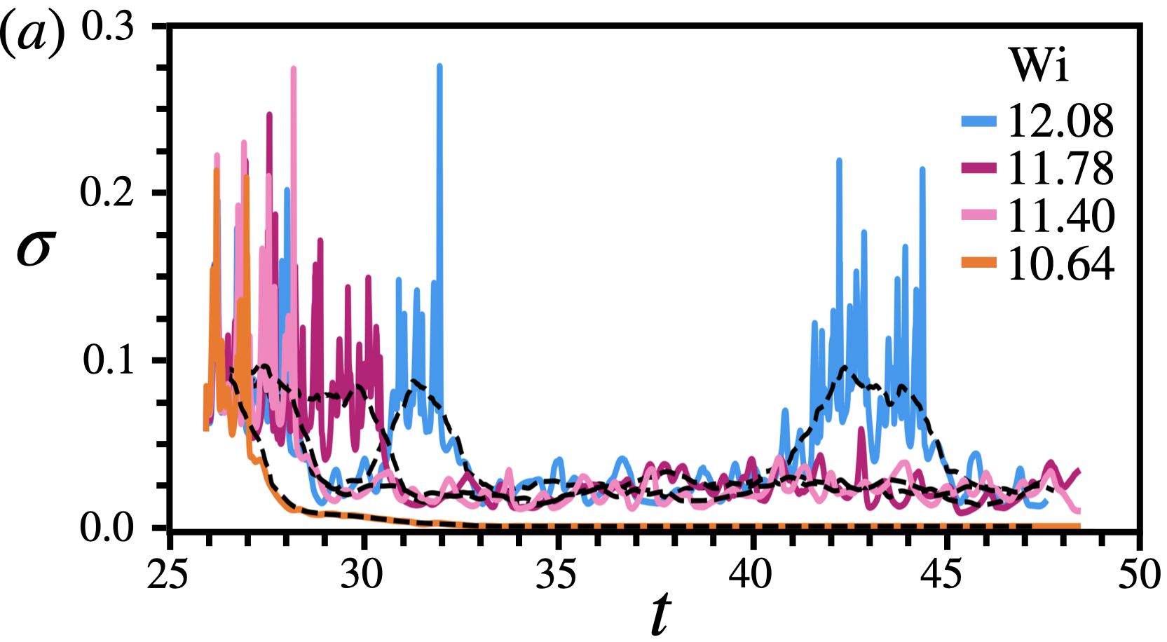
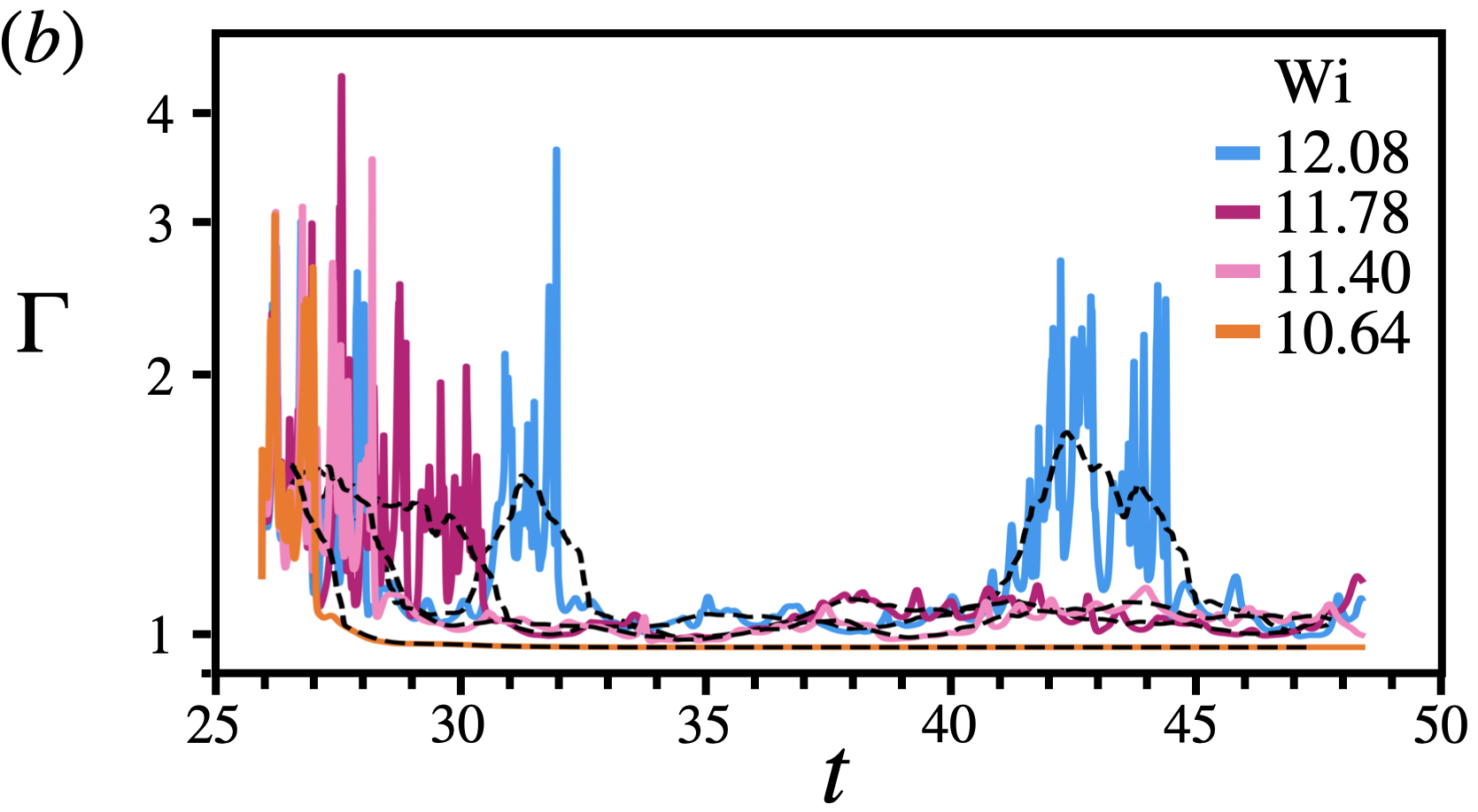
Figure 11: (a) Secondary-flow strength $\sigma$ and (b) flow resistance $\Gamma$ (log scale) as a function of time $t$ for different $\mathrm{Wi}$ when the flow is initialized in the turbulent state. In both cases the fluid flow is simulated at $\mathrm{Wi}$ = 15.96 for the first 26 rotations and then $\mathrm{Wi}$ is lowered to the indicated values.

III.3.5 Hysteretic behavior

Subcritical transitions can show hysteretic behavior. To explore this further, we perform simulations which start in the turbulent flow state at a high Weissenberg number and subsequently lower its value. The simulations are initialized at $\mathrm{Wi}$ $=15.96$ for $t=26$ rotations. Afterwards the Weissenberg number is lowered to $\mathrm{Wi}=12.084,11.78,11.4$ and $10.64$ for the next $t=22$ rotations. The resulting secondary-flow strength is plotted in Fig. 11 (a) as a function of time. We observe three different responses: bistable flow, hysteretic behavior, and laminar flow. The bistable regime is observed at $\mathrm{Wi}$ = 12.084. The secondary-flow strength $\sigma$ initially remains in the turbulent state for 3 rotations. Then, the flow becomes weakly chaotic for less than 2 rotations and switches back to the turbulent branch for about 2 rotations and back to the weakly chaotic flow again. After a more quiescent episode of about 10 rotations the turbulent state is entered and so on. The order parameters of the two flow states, $\Phi_{\mathrm{d}}^{\mathrm{I}}$ and $\Phi_{\mathrm{d}}^{\mathrm{II}}$, are displayed by the open circles and triangles in Fig. 8, respectively.

At lower Weissenberg numbers, $\mathrm{Wi}$ = 11.78 and $\mathrm{Wi}$ = 11.4, below $\mathrm{Wi}_{c}$ clear hysteretic behavior is observed. The secondary-flow strength drops from the initial turbulent state to the weakly chaotic flow state and stays there for the duration of the simulation (see also the order parameter $\Phi_{\mathrm{d}}$ given by the open triangles in Fig. 8). In contrast, in simulations starting from a resting fluid the flow remains laminar with a small secondary-flow strength of about $\sigma=0.025$ (see Sec. III.3.2 and Fig. 8). Finally, at the lowest Weissenberg number, $\mathrm{Wi}$ = 10.64, the flow becomes laminar with a secondary-flow strength $\sigma\ll 1$.

Moreover, we also study the hysteretic behavior in the flow resistance $\Gamma$, the total work performed on the viscoelastic fluid per unit time and unit volume, which is plotted in Fig. 11(b). Similar to the secondary-flow strength, the same three responses are observed. In the bistable flow state, the strongly fluctuating $\sigma$ and $\Gamma$ are clearly correlated, while for the weakly chaotic flow both quantities are small. Finally, in the laminar state, $\sigma\ll 1$, $\Gamma\leq 1$ and both quantities are constant in time. Note that experiments performed with the von Kármán flow geometry also demonstrate hysteretic behavior Groisman and Steinberg (2000, 2004); Burghelea, Segre, and Steinberg (2007); McKinley et al. (1991). The total work performed on the fluid shows hysteresis in the range $7<$$\mathrm{Wi}$ $<15$ Burghelea, Segre, and Steinberg (2007). However, above $\mathrm{Wi}$ $=18$, square-root scaling of the flow resistance is observed in these experiments, which we do not capture in our simulations where the flow resistance only shows a small increase.

We add an interesting observation about the spatial and temporal evolution of the elastic stress for the case $\mathrm{Wi}=10.64$, where the flow field develops from the full turbulent to the laminar base state. In the turbulent state, initialized at $\mathrm{Wi}=15.96$, many spatial modes are excited, which after lowering $\mathrm{Wi}$ will decay. We expect the least stable mode to decay the slowest and hence be the longest present, before the base flow is reached. We present the spatial and temporal evolution of the color-coded elastic stress component $\tau_{\phi\phi}$ in the $z-\phi$ plane near the outer cylinder ($r=0.99\,r_{o}$) in the video attached to Fig. 12 (Multi media view) for $\mathrm{Wi}=10.64$. The video comprises the time range, where Fig. 11(a) indicates that the disturbance flow has vanished. Interestingly, we still observe a weak disturbance flow corresponding to a non-axisymmetric mode with wave number $m=\pm 3$ as the least stable mode. In contrast, when starting the simulations with the fluid at rest, the system settles directly into the base flow. The observed mode agrees with our linear stability analysis (see Sec. III.1), where we predicted $|m|=3$ as the most unstable mode. Even the predicted critical Weissenberg number fits to the numerical results. The laminar state is recovered at $\mathrm{Wi}=10.64<\mathrm{Wi_{c}^{LSA}}=11.255$ and the flow state remains weakly chaotic at $\mathrm{Wi}=11.40>\mathrm{Wi_{c}^{LSA}}=11.255$.

Now, we study the spatio-temporal evolution of the elastic stress component $\tau_{\phi\phi}$ for $\mathrm{Wi}=11.40$, where the weakly chaotic flow regime occurs. It is shown in the video attached to Fig.  12(b) (Multi media view). Beyond $t=29.4$ the video shows, on average, a dynamic pattern with three-fold symmetry. This nicely supports our linear-stability analysis and the prediction of the unstable $|m|=3$ mode beyond $\mathrm{Wi_{c}^{LSA}}=11.255$.

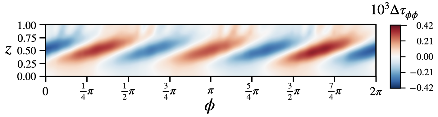
Figure 12: (Multimedia view) Azimuthal stress-tensor component color-coded in the $z-\phi$ plane near the outer radius $r=0.99\,r_{o}$ at $\mathrm{Wi}=10.64$. The component $\Delta\tau_{\phi\phi}=\tau_{\phi\phi}-\overline{\tau_{\phi\phi}}|_{t_{s}}^{t_{e}}$ is given relative to the mean value calculated between times $t_{s}=46$ and $t_{e}=48$. The snapshot of the stress field is taken at time $t=37.16$.

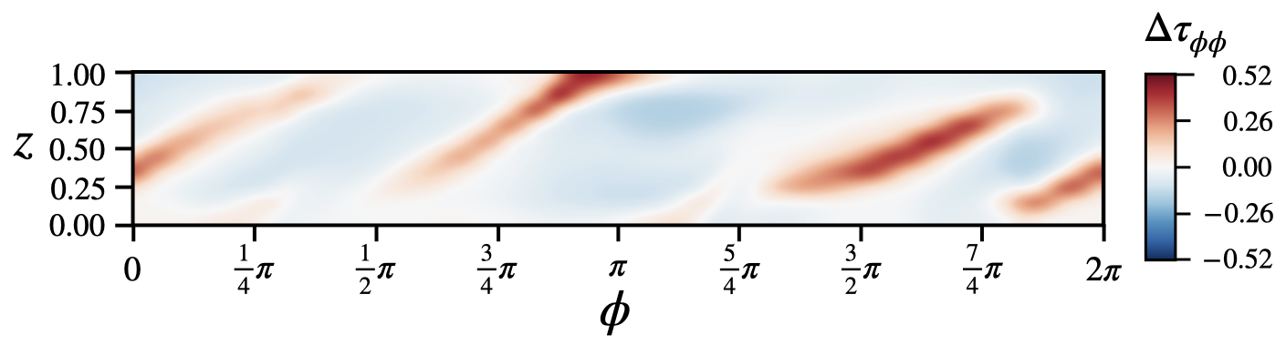
Figure 13: (Multimedia view) Azimuthal stress-tensor component color-coded in the $z-\phi$ plane near the outer radius $r=0.99\,r_{o}$ at $\mathrm{Wi}=11.40$. The component $\Delta\tau_{\phi\phi}=\tau_{\phi\phi}-\overline{\tau_{\phi\phi}}|_{t_{s}}^{t_{e}}$ is given relative to the mean value calculated between times $t_{s}=46$ and $t_{e}=48$. The snapshot of the stress field is taken at time $t=29.4$.

III.4 Power spectral density

An important feature of elastic turbulence is the characteristic power-law dependence of the spatial and temporal power spectral densities of the velocity fluctuations. We denote them by $\mathcal{P}_{s}(m)$ and $\mathcal{P}_{t}(f)$, respectively. In this section, we first discuss the temporal power spectra and secondly the spatial power spectra of the velocity fluctuations.

III.4.1 Temporal

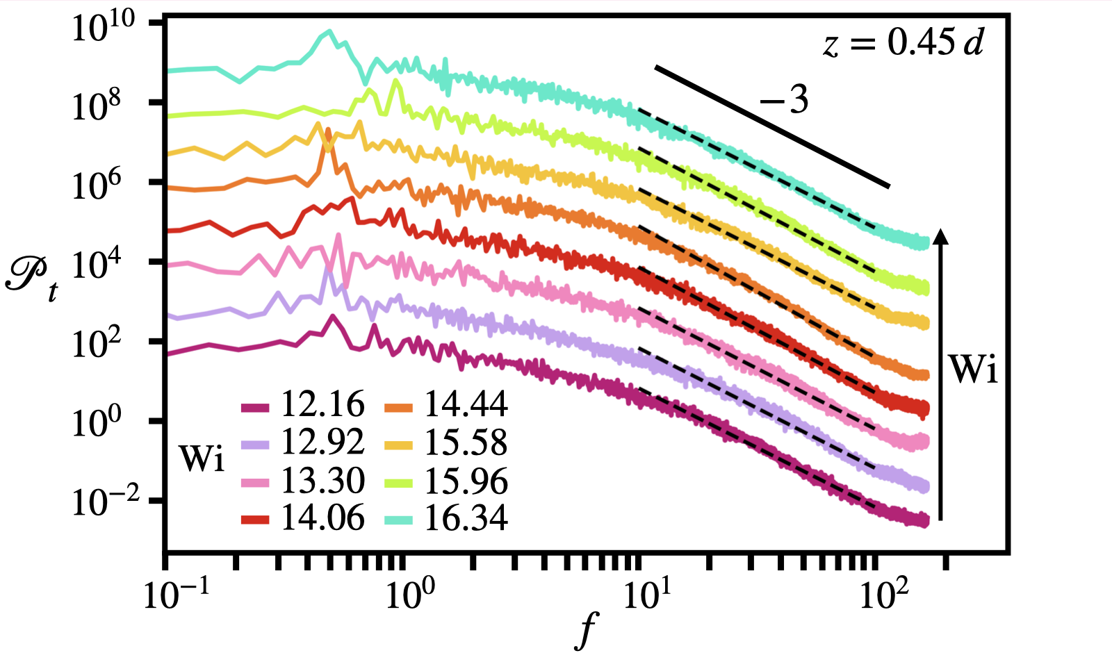
Figure 14: Temporal power spectral density $\mathcal{P}_{t}(f)=\langle|\mathcal{F}\{\bm{u}\}(f)|^{2}\rangle_{\phi}$ of the velocity fluctuations as a function of the frequency $f$ for different $\mathrm{Wi}$. The spectra are taken at height $z=0.45\,d$ and radial position $r=0.99\,r_{o}$. The data are arbitrarily offset for clarity by multiplying with a constant. Power laws $f^{-\alpha_{t}}$ are fitted and plotted as black dashed lines in the frequency range $9.92\leq f\leq 99.2$.

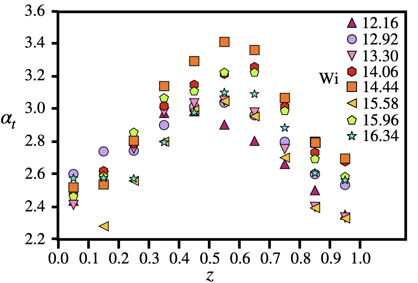
Figure 15: Temporal exponent $\alpha_{t}$ plotted versus the height $z$ for several values of the Weissenberg number $\mathrm{Wi}$ above $\mathrm{Wi}_{c}=12$. The exponents are obtained from the slope of the power spectra $\mathcal{P}_{t}(f)$ at radius $r=0.99\,r_{o}$.

The temporal power spectral density of the velocity field $\mathcal{P}_{t}(f)=\langle|\mathcal{F}\{\bm{u}\}(f)|^{2}\rangle_{\phi}$ is plotted in Fig. 14 versus the frequency $f$ for various values of the Weissenberg number in the range $12<\mathrm{Wi}<18$. Here, $\mathcal{F}\{\bm{u}\}$ denotes the temporal Fourier transform of the velocity field $\bm{u}$ and $\langle\dots\rangle_{\phi}$ indicates the average over the azimuthal angle, which we perform due to the angular symmetry of the geometry. We observe that the fluctuations in the fluid flow are strongest near the edge of the outer cylinder and in the midplane of the parallel plate geometry. Therefore, the power spectra are taken at radius $r=0.99\,r_{o}$ and height $z=0.45\,d$.

All the energy spectra in Fig. 14 are plotted for Weissenberg numbers above $\mathrm{Wi}_{c}$. We observe a gradual decrease at low $f$ and a steep decline between $f\approx 10$ and $f\approx 100$. It can be fitted by a power-law decay $\mathcal{P}_{t}(f)\propto f^{-\alpha_{t}}$ as the dashed lines indicate. The power-law spectrum hints at a randomly fluctuating velocity flow field in time, where most temporal frequencies are excited and correlations decrease fast. Fitting the temporal exponent $\alpha_{t}$, we observe $2.99\leq\alpha_{t}\leq 3.30$ for all $\mathrm{Wi}\leq 16.34$. Our largest value for $\alpha_{t}$ is comparable to the values of $\alpha_{t}=3.5$ and $3.6$ found in experiments on the parallel plate geometry Groisman and Steinberg (2000, 2004).

Furthermore, the characteristic exponent $\alpha_{t}$ also depends on the height $z$. We show this dependence for different $\mathrm{Wi}$ in Fig. 15. A clear increase of $\alpha_{t}$ towards the midplane in the two-plate geometry is observed due to increased velocity fluctuations. Additionally, $\alpha_{t}$ shows non-monotonic behavior in $\mathrm{Wi}$. It first increases after the transition at $\mathrm{Wi}_{c}$ and then decreases for $\mathrm{Wi}>14.44$.

III.4.2 Spatial

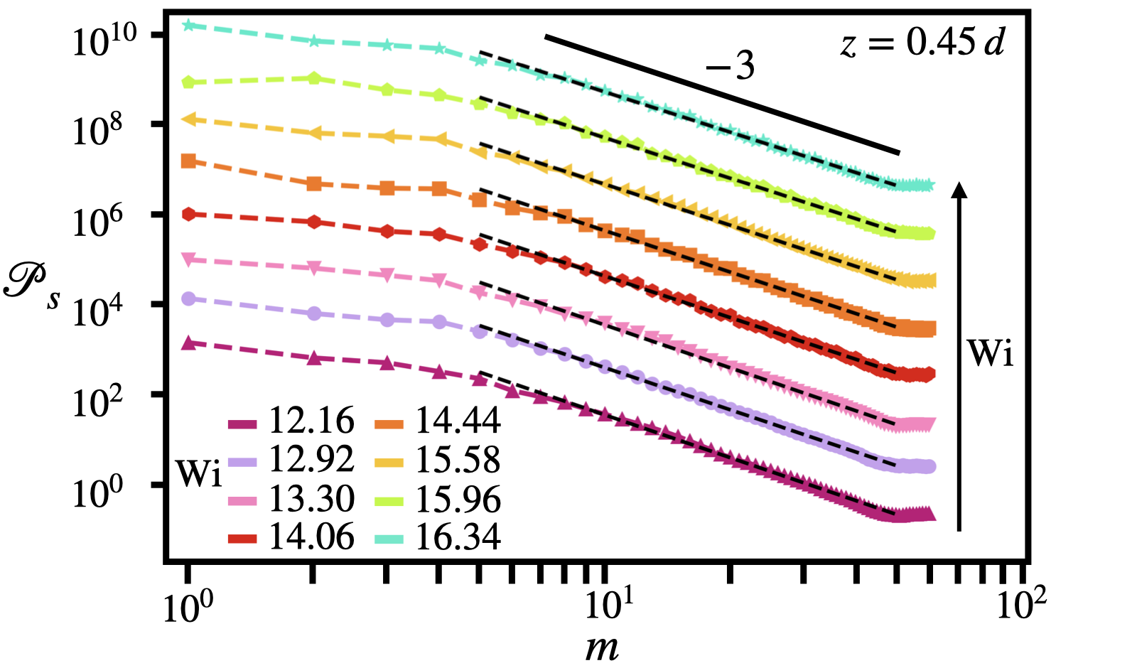
Figure 16: Spatial power spectral density $\mathcal{P}_{s}(m)=\overline{|\mathcal{F}\{\bm{u}\}(m)|^{2}}$ of the velocity fluctuations as a function of the azimuthal wave number $m$ for different $\mathrm{Wi}$. The spectra are taken at height $z=0.45\,d$ and radial position $r=0.99\,r_{o}$. The data are arbitrarily offset for clarity by multiplying with a constant. Power laws $m^{-\alpha_{s}}$ are fitted and plotted as black dashed lines in the range $5\leq m\leq 50$.

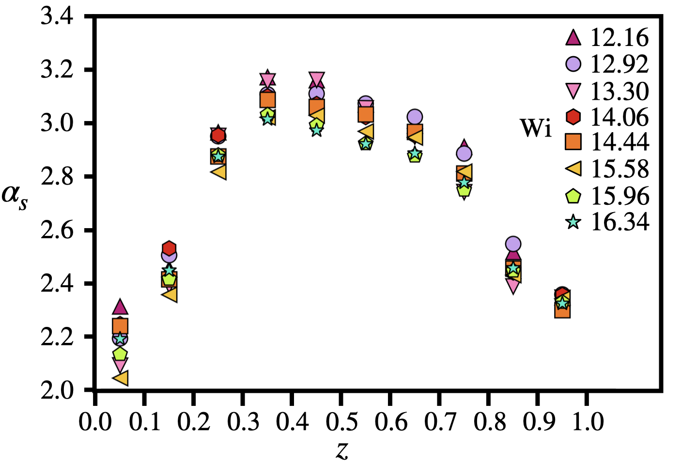
Figure 17: Spatial characteristic exponent $\alpha_{s}$ plotted versus the height $z$ for several values of the Weissenberg number $\mathrm{Wi}$ above $\mathrm{Wi}_{c}=12$. The exponents are obtained from the slope of the power spectra $\mathcal{P}_{s}(m)$ at radius $r=0.99\,r_{o}$.

In Fig. 16 we plot the spatial power spectra of the velocity field $\mathcal{P}_{s}(m)=\overline{|\mathcal{F}\{\bm{u}\}(m)|^{2}}$ along the azimuthal direction against the azimuthal wave number $m$ for several $\mathrm{Wi}>\mathrm{Wi}_{c}$. Again, we determine the spectra at radius $r=0.99\,r_{o}$ and height $z=0.45\,d$ and the bar indicates the temporal average. We observe a monotonic decrease in energy density with increasing azimuthal mode $m$ in all power spectra. The energy located in the first four modes is nearly constant while beyond $m=4$ it sharply decreases with $m$ according to the power law $\mathcal{P}_{s}(m)\sim m^{-\alpha_{s}}$, where $\alpha_{s}$ is the spatial exponent. The dashed lines are fits in order to determine $\alpha_{s}$. In Fig. 17 we plot the spatial exponent $\alpha_{s}$ versus height $z$ for different $\mathrm{Wi}$. The exponent $\alpha_{s}$ shows similar behavior as its temporal counterpart. It is smallest near the upper and lower plate and largest in the midplane of the geometry, for all Weissenberg numbers above the transition. This behavior is again consistent with our observation that the largest velocity fluctuations occur in the midplane. For $0.3<z<0.7$, the exponent $\alpha_{s}$ is larger than 3 in agreement with the theoretical condition for elastic turbulence derived in Ref. Fouxon and Lebedev, 2003. Our maximum value of $\alpha_{s}=3.16$ at $z=0.45$ and $\mathrm{Wi}=12.16$ or $\mathrm{Wi}=13.30$ is again close to the experimentally observed value of $\alpha_{s}=3.5$ Burghelea, Segre, and Steinberg (2007).

The overall trend of both temporal and spatial exponents is similar as well as the maximum values of both exponents. However, the spread of values in the temporal exponent is much larger than in the spatial exponents, which are all grouped closely together, indicating that the spatial exponents are more accurate. Our results suggest that Taylor’s hypothesis for inertial turbulence, according to which both exponents should be equal Taylor (1938), is not completely fulfilled in our simulations. However, the difference between the exponents is small and the behavior of both exponents as a function of the height is remarkably close, which implies that also applying Taylor’s hypothesis to elastic turbulence is often reasonable.

IV Discussion: Comparison to experiments

In our work, we did not aim to quantitatively reproduce the results of a specific experiment on the van Kármán swirling flow. Instead, due to the numerical complexity we first present an investigation of the general features of the elastic instability and elastic turbulence, as we observe them in our simulations. In the following we discuss our findings also in the context of experimental results.

IV.1 Geometric parameters

We first note that even a dilute polymer solution can exhibit complex behavior, which is not captured by the Oldroyd-B model, an idealized polymeric fluid model. This includes shear thinning, viscous heating, polymer degradation, finite polymer extensibility, and a broad spectrum of relaxation times. Thus a detailed comparison with experiments is hard at this stage. We therefore decided to use the Oldroyd-B model to capture main features of the elastic instability and elastic turbulence.

Moreover, we implemented a lateral boundary condition, where we allow tangential flow, while in experiments lateral walls with no-slip boundary conditions are used to constrain the fluid. There, the distance between the rotating plate and the lateral wall is an important parameter, especially when the distance becomes small. This creates high shear gradients in the corner between the rotating plate and the static wall. As a result, a secondary flow with curved streamlines can arise such as in the case of the Taylor-Couette geometry Davoodi et al. (2018). Our aim was to avoid such complications.

Finally, the aspect ratio of plate radius to plate separation influences the transitional path to elastic turbulence McKinley et al. (1991). We chose a large value to achieve a more uniform shear rate along the gap between the plates and to obtain a linear shear profile in the radial direction. Since the largest shear rate occurs at the lateral sides of the swirling flow, the elastic instability first occurs there.

IV.2 Onset of the instability

In experiments radially localized disturbances become visible at the critical Weissenberg number McKinley et al. (1991); Schiamberg et al. (2006). They are described by the linear stability analysis of Ref. Öztekin and Brown, 1993, which shows that the critical Weissenberg number and the azimuthal wave number $m$ of the most unstable mode depends on different parameters such as the gap-to-plate-radius ratio, Deborah number, and the viscosity ratio $\beta$. Furthermore, experiments show that depending on the different parameters, the elastic instability can be either continuous or hysteretic Schiamberg et al. (2006); Burghelea, Segre, and Steinberg (2007).

Following the approach of Ref. Öztekin and Brown, 1993, we derived a corrected set of equations, from which we identified the non-axisymmetric mode with three-fold symmetry to be the most unstable at the critical value $\mathrm{Wi_{c}^{LSA}}=11.255$. Other non-axisymmmetric modes with two- and four-fold symmetries and the axisymmetric mode become unstable slightly above $\mathrm{Wi}=12$, all with radial wave numbers $\alpha$ between 3.25 and 3.5. Shallow minima in the corresponding neutrality curves in the $\alpha-\mathrm{Wi}$ plane indicate that many modes with similar $\alpha$ become unstable at the same Weissenberg number. In contrast, in our simulations near the transition, we observe an unstable non-axisymmetric mode with four-fold symmetry, which drives the laminar flow towards weakly chaotic and turbulent flow. It develops at the outer edge of the swirling flow, where the shear rate is the highest. This observation agrees well with experiments McKinley et al. (1991); Schiamberg et al. (2006) and corresponds to the localized radial position assumed in the linear stability analysis. The discrepancy between simulations and the linear stability analysis is most likely due to the fact that the latter uses spatial decoupling in the ansatz for the flow field and considers flow between infinitely extended parallel plates.

Our subcritical transition displays hysteretic behavior, which has also been observed in experiments Groisman and Steinberg (2000, 2004); Burghelea, Segre, and Steinberg (2007); McKinley et al. (1991). When we now lower $\mathrm{Wi}$ below the critical value $\mathrm{Wi_{c}}=12$, the remaining weakly chaotic flow fluctuates around a three-fold symmetric pattern ($|m|=3$). Ultimately, further lowering $\mathrm{Wi}$ below $\mathrm{Wi_{c}^{LSA}}$ we observe a clear non-axisymmetric mode, which decays to zero, in good agreement with our linear stability analysis. What we do not understand is why the $|m|=3$ mode does not develop from the base flow, when we increase $\mathrm{Wi}$. A possible reason is that this requires much longer simulations, which we cannot perform. Note also in the experiments of Ref. Magda and Larson, 1988 a long duration of ca. $2100\,\mathrm{s}\approx 100\,\lambda$ was needed to observe the elastic instability.

IV.3 Bistable flow state and order parameter

In experiments different transition paths are observed beyond the critical Weissenberg number. Either the first transition is subcritical into a non-axisymmetric single mode followed by elastic turbulence Burghelea, Segre, and Steinberg (2007) or a sequence of continuous transitions between periodic and aperiodic modes occurs before elastic turbulence is entered Schiamberg et al. (2006). In constrast, in our simulations above the critical Weissenberg number, a bistable flow state emerges, which has not been reported so far in experiments. The weakly chaotic flow displays small velocity fluctuations around a small mean value $\langle\sigma\rangle\approx 0.02$ and the turbulent flow shows large velocity fluctuations around a larger mean value of $\langle\sigma\rangle\approx 0.1$. When $\mathrm{Wi}$ is closer to $\mathrm{Wi}_{c}$, the bistable flow state needs more time to develop from the laminar base flow. This was also observed in experimentsMcKinley et al. (1991).

IV.4 Flow resistance

In accordance with the subcritical transition from laminar base flow to the non-axisymmetric mode, the experiments in Ref. Burghelea, Segre, and Steinberg, 2007 also observe a sharp increase in the flow resistance and hysteresis. This agrees with the numerical findings in our work. The flow resistance sharply increases at the transition by a factor of 1.4 and shows hysteresis. The increase is mainly due to the turbulent flow and work performed on the open side surface of the swirling flow, while the contribution from the weakly chaotic flow gradually increases starting at $\mathrm{Wi}_{c}$. Particularly, the elastic part of the work outweighs the viscous part, which demonstrates the elastic nature of the transition. Note that in experiments performed on swirling flows with a fixed outer boundary Groisman and Steinberg (2000, 2001a, 2001b, 2004); Burghelea, Segre, and Steinberg (2007); Jun and Steinberg (2009, 2017); Schiamberg et al. (2006) all work is solely performed on the top surface of the fluid and the increase in the flow resistance is directly measurable by the work required to rotate the top plate. Finally, in experiments in the regime of elastic turbulence the flow resistance shows power law scaling with an exponent of 0.49 Burghelea, Segre, and Steinberg (2007), while we only observe a small increase.

IV.5 Power spectrum spatial and temporal

In experiments the temporal power spectra of the velocity fluctuations are measured in the center of the swirling flow Groisman and Steinberg (2000, 2004); Burghelea, Segre, and Steinberg (2007), where velocity fluctuations are assumed to be homogeneous and isotropic. Our spatial power spectra along the azimuthal direction can only be determined outside the center for $r\neq 0$. Since in our case velocity fluctuations are largest at the open side surface of the swirling flow, we decided to record the spectra near this location. While the velocity fluctuations become anisotropic, we do not expect the scaling exponents to strongly change since we always use the magnitude of the Fourier transformed velocity vector, when determining the spectra.

In the turbulent flow state, similar to experiments, we also observe power-law scaling in the spatial and temporal power spectral densities. The power spectra were analyzed at different heights $z$ between the two plates. The steep decay observed in the spatial power spectra shows that the magnitude of velocity fluctuations occurring at large spatial modes is greatly reduced and velocity fluctuations mainly occur on large spatial scales (on the order of the system size). Hence, the velocity field is spatially smooth, dominated by strong nonlinear interactions of a few large-scale spatial modes Steinberg (2021). In the height range $0.3<z<0.7$, we find the spatial scaling exponent $\alpha_{s}$ in $\mathcal{P}_{s}(m)\sim m^{-\alpha_{s}}$ to be above 3, which is a determining feature of elastic turbulence Fouxon and Lebedev (2003). Both, spatial and temporal exponents show similar behavior as a function of the height $z$ and are largest in the midplane, where velocity fluctuations are largest. The maximum values of the temporal ($\alpha_{t}=3.41$) and spatial ($\alpha_{s}=3.17$) exponents in our simulations are remarkably close to the experimentally observed values Groisman and Steinberg (2000, 2004); Burghelea, Segre, and Steinberg (2007). Since both exponents show the same behavior as a function of the height $z$ and their values are similar, our results suggest that applying Taylor’s hypothesis to numerical solutions displaying elastic turbulence is usually reasonable.

V Conclusion

In summary, we have presented a detailed analysis of the three-dimensional von Kármán swirling flow between two parallel plates through numerical solutions of the Oldroyd-B model. We characterized the flow state with the secondary-flow strength $\sigma$, a measure of the average strength of the velocity fluctuations, and then defined an order parameter $\Phi$ as the time average of $\sigma$. At the critical Weissenberg number $\mathrm{Wi_{c}}=12$, the order parameter displays a subcritical transition from laminar flow to a bistable flow, which switches between weakly chaotic flow, where $0.01<\Phi<0.06$, and elastic turbulence with $\Phi>0.07$. We defined the flow resistance as the total work performed on the fluid and found a significant increase of the flow resistance at the transition, due to the elastic part of the fluid in the turbulent flow state. In addition, we observed hysteretic behavior in both the secondary-flow strength and the flow resistance, which is a common feature of a subcritical transition and has also been found in experiments Groisman and Steinberg (2000, 2004); Burghelea, Segre, and Steinberg (2007); McKinley et al. (1991). Furthermore, we analyzed the spatial and temporal power spectra of the velocity field. Their power-law decays reflect the turbulent nature of the flow. Overall, we observe a different transitional route to elastic turbulence than in the experiments of Groisman and Steinberg Groisman and Steinberg (2000, 2004), Burghelea et al. Burghelea, Segre, and Steinberg (2007) and Schiamberg et al. Schiamberg et al. (2006). However, the observed properties of elastic turbulence remain similar.

Our numerical simulation study helps to further understand the transition from laminar to turbulent flow and to characterize viscoelastic fluid flow beyond the transition. In particular, we are able to monitor physical quantities such as the elastic stress fields, which are not directly accessible in experiments. However, polymer solutions used in the experiments have more complex behavior than the relatively simple Oldroyd-B model. Several directions exist to extend our investigations. More detailed numerical work is recommended to investigate the elastic instability near the transition from laminar to chaotic or turbulent flow. In particular, studies involving varying the ratio of plate radius to plate distance and the polymer-to-solvent viscosity ratio are warranted. Also, more refined polymer models that include shear thinning and/or finite polymer extensibility, such as the FENE-P model, should be studied. However, detailed parameter studies are still limited due to the large computational effort and the large amount of data storage required. Moreover, the influence of different boundary conditions of the swirling flow at its lateral side has to be analyzed further, both numerically and experimentally. Also, a nonlinear stability analysis of the instability, which has not yet been performed, could further illuminate the transition. One important characteristic of elastic turbulence, the interesting application of mixing solutes by elastic turbulent flow, has not been inspected in simulations, yet. We aim to address some of these open questions in future work.

Author Contributions

All authors contributed equally to this work.

Conflict of Interest

The authors have no conflicts to disclose.

Data Availability Statement

The data that support the findings of this study are available from the corresponding author upon reasonable request.

Appendix A Spatial mesh

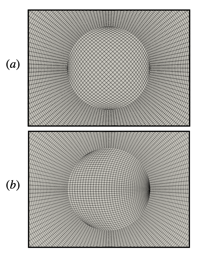
Figure 18: Overview of the inner cylinder block comprising a square-like lattice employed in the simulations. The faces are connected to the mesh of the the outer cylinder, which is constructed from (a) four connected trapezoid blocks and (b) three connected trapezoid blocks.

Here we give a brief description of the special square-like mesh employed in the inner cylindrical block to avoid the singularity at $r=0$. The internal matching of the cells leads to small mesh volumes (visible by dark regions in Fig. 18), which in turn lead to small numerical errors on the order of $0.0013\,u^{0}_{\mathrm{max}}$, where $u^{0}_{\mathrm{max}}=r_{o}\Omega$ is the maximum base flow velocity. The numerical errors have the same spatial symmetry as the symmetry of the connected trapezoid blocks comprising the outer cylinder. To check the accuracy of the four-fold azimuthal pattern developing (see Sec. III.2), we performed simulations with the outer cylinder consisting out of four and out of three connected blocks, see Fig. 18. For both meshes we find a four-fold symmetric unstable mode.

Appendix B Initial disturbance wave

Here we display the onset of the instability from a different perspective. The onset is equivalent to the one described in Sec. III.2. We first observe an initial axisymmetric disturbance flow, which begins at the outer edge and then travels inwards, see Fig. 19. In the figure, the axisysmmetric elastic wave can be seen traveling inwards at the outer edge with snapshots given in Fig. 19 (a)-(c) with increasing time. Afterwards, an unstable non-axisymmetric mode with azimuthal wave numbers $m=\pm 4$ develops which drives the flow towards weakly chaotic flow (shown in the video) and ultimately towards elastic turbulence (not shown in the video).

Figure 19: (Multimedia view) Azimuthal stress-tensor component color-coded in the $r-\phi$ plane near the mid plane $z=0.45\,d$ at $\mathrm{Wi}=12.008$. The component $\Delta\tau_{\phi\phi}=\tau_{\phi\phi}-\overline{\tau_{\phi\phi}}|_{t_{s}}^{t_{e}}$ is given relative to the mean value between times $t_{s}=2$ and $t_{e}=12$. Snapshots of the stress field are taken at times: (a) $t=1.2$, (b) $t=1.85$ and (c) $t=2.44$. An axisymmetric disturbance is observed, which travels inwards and decays over time.

Appendix C Linear Stability Analysis

In our linear stability analysis we perform a classical normal-mode perturbation, following the work of Ref. Avgousti and Beris, 1993 and Öztekin and Brown, 1993. We decouple the spatial dependencies of the perturbation and superimpose an infinitesimal disturbance ($\bm{\tau}^{\prime},\bm{u}^{\prime},p^{\prime}$) on the base flow solution ($\bm{\tau}^{0},\bm{u}^{0},p^{0}$). We further consider an infinitely extended flow in the radial direction, which is bounded between two plates in the z-direction. The perturbation is assumed to occur at a critical radius $r_{c}$, where the Weissenberg number reaches its critical value: $\mathrm{Wi}_{c}=\lambda\Omega r_{c}/d$. We set the top plate at $z=1$ fixed and the lower plate at $z=0$ to be moving with angular velocity $\Omega$. Neglecting fluid inertia ($\text{Re}\approx 0$), the steady-state velocity field for infinitely extended parallel plates is purely azimuthal and given by

$$\bm{u}^{0}=\frac{r\Omega}{d}(1-z)\bm{e}_{\phi}\,.$$ (24)

The corresponding base stress and pressure fields read

$$\tau_{rr}^{0}=\tau_{r\phi}^{0}=\tau_{rz}^{0}=\tau_{zz}^{0}=0;\qquad\tau_{\phi z}^{0}=-\eta_{p}\frac{r\Omega}{d};$$ (25)

$$\tau_{\phi\phi}^{0}=2\eta_{p}\lambda\left(\frac{r\Omega}{d}\right)^{2};\qquad p^{0}=-\eta_{p}\lambda\left(\frac{r\Omega}{d}\right)^{2}\,.$$ (26)

The velocity, stress and pressure fields are then expressed as

$$\tilde{\bm{\tau}}=\bm{\tau}^{0}+\bm{\tau}^{\prime}\,;\qquad\bm{\tilde{u}}=\bm{u}^{0}+\bm{u}^{\prime}\,;\qquad\tilde{p}=p^{0}+p^{\prime}\,.$$ (27)

After substituting Eq. (27) in the governing equations (1)-(3), subtracting the base flow given by the velocity field Eq. (24), stress and pressure fields Eq. (25) and keeping only terms that are linear in the disturbance functions, we obtain a set of 10 ordinary differential equations described in the following. Dimensionless variables are obtained by normalizing the length by $d$, the time by $\Omega^{-1}$, the velocity by $d\Omega$ and the stress by $(\eta_{s}+\eta_{p})\Omega$. We denote the dimensionless variables by $(r,\phi,z)$ and obtain for the continuity equation,

$$\frac{1}{r}\frac{\partial\,r\,u_{r}}{\partial r}+\frac{1}{r}\frac{\partial u_{\phi}}{\partial\phi}+\frac{\partial u_{z}}{\partial z}=0\,,$$ (28)

the three linearized momentum equations,

$$\frac{1}{r}\frac{\partial}{\partial r}\left(r\tau_{rr}\right)+\frac{1}{r}\frac{\partial\tau_{r\phi}}{\partial\phi}+\frac{\partial\tau_{rz}}{\partial z}-\frac{\tau_{\phi\phi}}{r}-\frac{\partial p}{\partial r}+\kappa\left(\nabla^{2}u_{r}-\frac{2}{r}\frac{\partial u_{\phi}}{\partial\phi}-\frac{u_{r}}{r^{2}}\right)=0\,,$$ (29)

$$\frac{\partial\tau_{r\phi}}{\partial r}+\frac{1}{r}\frac{\partial\tau_{\phi\phi}}{\partial\phi}+\frac{\partial\tau_{\phi z}}{\partial z}+2\frac{\tau_{r\phi}}{r}-\frac{1}{r}\frac{\partial p}{\partial\phi}+\kappa\left(\nabla^{2}u_{\phi}+\frac{2}{r^{2}}\frac{\partial u_{r}}{\partial\phi}-\frac{u_{\phi}}{r}\right)=0\,,$$ (30)

$$\frac{1}{r}\frac{\partial}{\partial r}\left(r\tau_{rz}\right)+\frac{1}{r}\frac{\partial\tau_{\phi z}}{\partial\phi}+\frac{\partial\tau_{zz}}{\partial z}-\frac{\partial p}{\partial z}+\kappa\nabla^{2}u_{z}=0\,,$$ (31)

where $\nabla^{2}$ is the Laplacian operator in cylindrical coordinates and $\kappa={\eta_{s}}/(\eta_{s}+\eta_{p})$, and six linearized stress constitutive equations

$$L(\tau_{rr}) =2\kappa_{p}\frac{\partial u_{r}}{\partial r}\,,$$ (32)

$$L(\tau_{r\phi})+\mathrm{De}\,r\tau_{rz}+\kappa_{p}\mathrm{De}\,r\left[\frac{\partial u_{r}}{\partial z}+2{\color[rgb]{0,0,0}\mathrm{De}}\left(u_{\phi}-\frac{\partial u_{r}}{\partial\phi}\right)\right] =\kappa_{p}\left(\frac{1}{r}\frac{\partial u_{r}}{\partial\phi}-\frac{u_{\phi}}{r}+\frac{\partial u_{\phi}}{\partial r}\right)\,,$$ (33)

$$L(\tau_{rz})+\kappa_{p}\mathrm{De}\,\left(\frac{\partial u_{r}}{\partial\phi}-u_{\phi}\right) =\kappa_{p}\left(\frac{\partial u_{r}}{\partial z}+\frac{\partial u_{z}}{\partial z}\right)\,,$$ (34)

$$L(\tau_{\phi\phi})+2\mathrm{De}\,r\tau_{\phi z}+2\kappa_{p}\mathrm{De}\,r\left[\frac{\partial u_{\phi}}{\partial z}-2{\color[rgb]{0,0,0}\mathrm{De}}\left(u_{r}+\frac{\partial u_{\phi}}{\partial\phi}\right)\right] =2\kappa_{p}\left(\frac{1}{r}\frac{\partial u_{\phi}}{\partial\phi}+\frac{u_{r}}{r}\right)\,,$$ (35)

$$L(\tau_{\phi z})+\mathrm{De}\,r\tau_{zz}+\kappa_{p}\mathrm{De}\,r\left(\frac{\partial u_{z}}{\partial z}+\frac{1}{r}\frac{\partial u_{\phi}}{\partial\phi}+\frac{u_{r}}{r}-2{\color[rgb]{0,0,0}\mathrm{De}}\frac{\partial u_{z}}{\partial\phi}\right) =\kappa_{p}\left(\frac{1}{r}\frac{\partial u_{z}}{\partial\phi}+\frac{\partial u_{\phi}}{\partial z}\right)\,,$$ (36)

$$L(\tau_{zz})+2\kappa_{p}\mathrm{De}\,\frac{\partial u_{z}}{\partial\phi} =2\kappa_{p}\frac{\partial u_{z}}{\partial z}\,,$$ (37)

where the operator $L\equiv[1+\mathrm{De}\,\partial/\partial t+\mathrm{De}\,(1-z)\partial/\partial\phi]$ and $\kappa_{p}=(1-\kappa)$. Here, we introduced the Deborah number, the ratio of the fluid relaxation time to the angular velocity of the rotating plate, $\mathrm{De}=\lambda\Omega$. The Weissenberg number is then given by $\mathrm{Wi}=\mathrm{De}\,r_{c}/d$.

Next, we insert the normal-mode perturbation and express the field equations by

$$\tilde{\bm{\tau}} =\bm{\tau}^{0}+\mathcal{R}\left[\bm{\tau}(z)\exp(i\alpha r+im\phi+\sigma t)\right]\,,$$ (38)

$$\bm{\tilde{u}} =\bm{u}^{0}+\mathcal{R}\left[\bm{u}(z)\exp(i\alpha r+im\phi+\sigma t)\right]\,,$$ (39)

$$\tilde{p} =p^{0}+\mathcal{R}\left[p(z)\exp(i\alpha r+im\phi+\sigma t)\right]\,,$$ (40)

where $\mathcal{R}[\dots]$ represents the real part, $\bm{\tau},\bm{u},p$ are complex infinitesimal functions of the z coordinate, $\alpha$ is the dimensional radial wave number, $m$ is the azimuthal wave number and $\sigma$ is the (in general) complex temporal eigenvalue. The azimuthal wave number $m$ is an integer, which can be positive or negative, corresponding to non-axisymmetric disturbances or zero, corresponding to axisymmetric disturbances.

After substituting Eq. (38)-(40) in our set of linearized equations Eq. (28)-(37), we obtain the following set of linear disturbance equations:

$$\left(\frac{1}{r}+i\alpha\right)u_{r}+\frac{im}{r}u_{\phi}+\frac{\partial u_{z}}{\partial z}=0\,,$$ (41)

$$\left(\frac{1}{r}+i\alpha\right)\tau_{rr}+\frac{im}{r}\tau_{r\phi}+\frac{\partial\tau_{rz}}{\partial z}-\frac{\tau_{\phi\phi}}{r}-i\alpha p+\kappa\left[\frac{\partial^{2}u_{r}}{\partial z^{2}}-(\alpha^{2}+m^{2})u_{r}-\frac{2im}{r}u_{\phi}-\frac{u_{r}}{r^{2}}\right]=0\,,$$ (42)

$$\left(\frac{2}{r}+i\alpha\right)\tau_{r\phi}+\frac{im}{r}\tau_{\phi\phi}+\frac{\partial\tau_{\phi z}}{\partial z}-\frac{im}{r}p+\kappa\left[\frac{\partial^{2}u_{\phi}}{\partial z^{2}}-(\alpha^{2}+m^{2})u_{\phi}+\frac{2im}{r^{2}}u_{r}-\frac{u_{\phi}}{r}\right]=0\,,$$ (43)

$$\left(\frac{1}{r}+i\alpha\right)\tau_{rz}+\frac{im}{r}\tau_{\phi z}+\frac{\partial\tau_{zz}}{\partial z}-\frac{\partial p}{\partial z}+\kappa\left[\frac{\partial^{2}u_{z}}{\partial z^{2}}-(\alpha^{2}+m^{2})u_{z}\right]=0\,,$$ (44)

$$\frac{1}{2}\mathcal{L}\tau_{rr} =i\alpha u_{r}\,,$$ (45)

$$\mathcal{L}\tau_{r\phi}+\mathrm{De}\,r\left(\frac{\tau_{rz}}{\kappa_{p}}-2im\mathrm{De}\,u_{r}+\frac{\partial u_{r}}{\partial z}\right) =\frac{im}{r}u_{r}+\left(i\alpha-\frac{1}{r}\right)u_{\phi}\,,$$ (46)

$$\mathcal{L}\tau_{rz}+im\mathrm{De}\,u_{r} =\frac{\partial u_{r}}{\partial z}+\frac{\partial u_{z}}{\partial z}\,,$$ (47)

$$\frac{1}{2}\mathcal{L}\tau_{\phi\phi}+\mathrm{De}\,r\left(\frac{\tau_{\phi z}}{\kappa_{p}}-2im\mathrm{De}\,u_{\phi}+\frac{\partial u_{\phi}}{\partial z}\right) =\frac{im}{r}u_{\phi}+\frac{u_{r}}{r}\,,$$ (48)

$$\mathcal{L}\tau_{\phi z}+\mathrm{De}\,r\left(\frac{\tau_{zz}}{\kappa_{p}}+\frac{im}{r}u_{\phi}-2im\mathrm{De}\,u_{z}+\frac{\partial u_{z}}{\partial z}\right) =\frac{im}{r}u_{z}+\frac{\partial u_{\phi}}{\partial z}\,,$$ (49)

$$\frac{1}{2}\mathcal{L}\tau_{zz}+im\mathrm{De}\,u_{z} =\frac{\partial u_{z}}{\partial z}\,,$$ (50)

where the linear operator $\mathcal{L}\equiv\kappa_{p}^{-1}[1+\mathrm{De}\,\sigma+im\mathrm{De}\,(1-z)]$.

Table 2: Real and imaginary parts of the most unstable eigenvalue $\sigma_{\mathrm{re}}$ and $\sigma_{\mathrm{im}}$, respectively, for axisymmetric (m=0) disturbances. The eigenvalue ${\color[rgb]{0,0,0}\sigma^{\mathrm{ref}}}$ is a nonzero solution to the equation $\psi^{\prime}={\color[rgb]{0,0,0}F^{\mathrm{ref}}}(z,\psi)$, the eigenvalue $\sigma$ is a nonzero solution to the equation $\psi^{\prime}=F(z,\psi)$ and $\sigma^{\mathrm{lit}}$ is the eigen value obtained from Ref. Öztekin and Brown, 1993. The axial wave number $\alpha=3.5$, the polymer to solvent viscosity ratio $\kappa=0.59,\beta=41/59\approx 0.695$, and the critical radius $r_{c}=5$. The number of collocation points is $N\geq 50$.

	Literature Öztekin and Brown (1993)		This work
$\mathrm{De}$	${\color[rgb]{0,0,0}\sigma_{\mathrm{re}}^{\mathrm{lit}}}$	${\color[rgb]{0,0,0}\sigma_{\mathrm{im}}^{\mathrm{lit}}}$	${\color[rgb]{0,0,0}\sigma_{\mathrm{re}}^{\mathrm{ref}}}$	${\color[rgb]{0,0,0}\sigma_{\mathrm{im}}^{\mathrm{ref}}}$	$\sigma_{\mathrm{re}}^{\mathrm{ref}}/\sigma_{\mathrm{re}}^{\mathrm{lit}}$	$\sigma_{\mathrm{re}}$	$\sigma_{\mathrm{im}}$
1	-0.53	-0.462	-0.50864	-0.44581	0.96	-0.47513	-0.48917
2	-0.036	-0.441	-0.02150	-0.42510	0.60	0.02226	-0.47436
3	0.12	-0.431	0.13430	-0.41470	1.12	0.18492	-0.46775
5	0.24	-0.4215	0.25322	-0.40508	1.06	0.30955	-0.45370

Table 3: Real and imaginary parts of the most unstable eigenvalue $\sigma_{\mathrm{re}}$ and $\sigma_{\mathrm{im}}$, respectively, for nonaxisymmetric ($m=1,2,3$) disturbances. The eigenvalue ${\color[rgb]{0,0,0}\sigma^{\mathrm{ref}}}$ is a nonzero solution to the equation $\psi^{\prime}={\color[rgb]{0,0,0}F^{\mathrm{ref}}}(z,\psi)$, the eigenvalue $\sigma$ is a nonzero solution to the equation $\psi^{\prime}=F(z,\psi)$ and $\sigma^{\mathrm{lit}}$ is the eigen value obtained from Ref. Öztekin and Brown, 1993. The Weissenberg number $\mathrm{Wi}=30$, the axial wave number $\alpha=3.5$, the polymer to solvent viscosity ratio $\kappa=0.59,\beta=41/59\approx 0.695$, and the critical radius $r_{c}=5$. The number of collocation points is $N\geq 50$.

	Literature Öztekin and Brown (1993)		This work
m	${\color[rgb]{0,0,0}\sigma_{\mathrm{re}}^{\mathrm{lit}}}$	${\color[rgb]{0,0,0}\sigma_{\mathrm{im}}^{\mathrm{lit}}}$	${\color[rgb]{0,0,0}\sigma_{\mathrm{re}}^{\mathrm{ref}}}$	${\color[rgb]{0,0,0}\sigma_{\mathrm{im}}^{\mathrm{ref}}}$	$\sigma_{\mathrm{re}}^{\mathrm{ref}}/\sigma_{\mathrm{re}}^{\mathrm{lit}}$	$\sigma_{\mathrm{re}}$	$\sigma_{\mathrm{im}}$
1	0.13	-1.25	0.13123	-0.77516	1.01	0.11270	-0.74802
2	0.17	-0.375	0.15170	-1.64974	0.89	0.24631	-1.47938
3	0.09	-0.345	0.07242	-2.60319	0.81	-0.07971	-2.61053

The set of linearized governing equations can be reduced from 10 independent variables to a set of 6 ordinary differential equations and 4 linear relationships. which we express with the vector

$${\color[rgb]{0,0,0}\bm{\psi}=[u_{r}(z),u_{\phi}(z),u_{z}(z),p(z),u_{r}^{\prime}(z),u_{\phi}^{\prime}(z)]^{\mathrm{T}}\,,}$$ (51)

where the prime indicates the derivative $g^{\prime}=dg/dz$ with respect to the spatial coordinate $z$. The boundary conditions of the perturbation are set to

$$\bm{u}(r,\phi,z)={\bm{0}}\qquad\text{at $z=0$ and $z=1$}\,.$$ (52)

Moreover, we take the radially localized perturbation to occur at the edge of the rotating cylinder, $r_{c}=r_{o}$, where the shear rate is the highest. Next, we numerically solve the linear stability problem using a collocation method, which discretizes the perturbation in the z direction with $N$ collocation points, with the computer algorithm solve_bvp available in the SciPy package Virtanen et al. (2020).

Next, we investigate the stability of the base flow with respect to axisymmetric disturbances ($m=0$) and to nonaxisymmetric disturbances ($0<m\leq 4$). First we validate our numerical algorithm and reproduce results of Ref. Öztekin and Brown, 1993, which is essential given the large number of terms involved in the calculations and our new approach to numerically solving them. In our derivation of the linearized set of equations, given by Eq. (28) - (37), we found extra terms compared to Ref. Öztekin and Brown, 1993. We observe two differences: in Eq. (28) the ${\partial u_{r}}/{\partial\phi}$ term scales with $\mathrm{De}^{2}$ instead of $\mathrm{De}$; and in Eqs. (28) - (37) we obtain terms involving $u_{r}$ and $u_{\phi}$, which are missing in Ref. Öztekin and Brown, 1993. Therefore, we will compare the results of both sets of equations. In the validation procedure we have tested the algorithm, where we solve the system of equations of Ref. Öztekin and Brown, 1993 defined as $\bm{\psi}^{\prime}={\color[rgb]{0,0,0}F^{\mathrm{ref}}}(z,\bm{\psi})$ to obtain the most unstable eigenvalue ${\color[rgb]{0,0,0}\sigma^{\mathrm{ref}}}$ for a specific Weissenberg number. We set the axial wave number to $\alpha=3.5$, the polymer to solvent viscosity ratio $\beta=41/59\approx 0.695$ (the polymer to total viscosity of the polymer solution ratio is $\kappa=0.4$), and the critical radius to $r_{c}=5$, which are the parameters used in Ref. Öztekin and Brown, 1993. The results for the axisymmetric case are presented in Table 2. The table shows good agreement between our algorithm and the results of Ref. Öztekin and Brown, 1993 for axisymmetric instabilities. Moreover, the most unstable eigenvalue of the newly derived set of equations $\sigma$ is close to the most unstable eigenvalue ${\color[rgb]{0,0,0}\sigma^{\mathrm{ref}}}$ of the former set of equations used in Ref. Öztekin and Brown, 1993.

In addition, the validation results for three nonaxisymmetric cases ($m=1,2,3$) are presented in Table 3 at Weissenberg number $\mathrm{Wi}$ = 3. Again, we see a good agreement between our algorithm and the results of Ref. Öztekin and Brown, 1993, where the deviation in the real part of sigma is at most 0.02 and the deviation in the imaginary part is about $0.5,1.3$, and $2.3$ for $m=1,2,3$, respectively. Thus, only for the imaginary part of the most unstable eigenvalue do we observe significant deviation. However, ${\sigma_{\mathrm{im}}}$ plays no role in the stability of the eigenvalue.

References

- Groisman and Steinberg (2000) A. Groisman and V. Steinberg, “Elastic turbulence in a polymer solution flow,” Nature 405, 53 (2000).
- Groisman and Steinberg (2004) A. Groisman and V. Steinberg, “Elastic turbulence in curvilinear flows of polymer solutions,” New J. Phys. 6, 29 (2004).
- Schiamberg et al. (2006) B. A. Schiamberg, L. T. Shereda, H. Hu, and R. G. Larson, “Transitional pathway to elastic turbulence in torsional, parallel-plate flow of a polymer solution,” J. Fluid Mech. 554, 191–216 (2006).
- Arratia et al. (2006) P. E. Arratia, C. C. Thomas, J. Diorio, and J. P. Gollub, “Elastic instabilities of polymer solutions in cross-channel flow,” Phys. Rev. Lett. 96, 144502 (2006).
- Groisman and Steinberg (2001a) A. Groisman and V. Steinberg, “Efficient mixing at low reynolds numbers using polymer additives,” Nature 410, 905 (2001a).
- Burghelea, Segre, and Steinberg (2007) T. Burghelea, E. Segre, and V. Steinberg, “Elastic turbulence in von karman swirling flow between two disks,” Phys. Fluids 19, 053104 (2007).
- Thomases and Shelley (2009) B. Thomases and M. Shelley, “Transition to mixing and oscillations in a Stokesian viscoelastic flow,” Phys. Rev. Lett. 103, 094501 (2009).
- Thomases, Shelley, and Thiffeault (2011) B. Thomases, M. Shelley, and J.-L. Thiffeault, “A stokesian viscoelastic flow: transition to oscillations and mixing,” Physica D 240, 1602–1614 (2011).
- Squires and Quake (2005) T. M. Squires and S. R. Quake, “Microfluidics: Fluid physics at the nanoliter scale,” Rev. Mod. Phys. 77, 977 (2005).
- Datta et al. (2021) S. S. Datta, A. M. Ardekani, P. E. Arratia, A. N. Beris, I. Bischofberger, J. G. Eggers, J. E. López-Aguilar, S. M. Fielding, A. Frishman, M. D. Graham, et al., “Perspectives on viscoelastic flow instabilities and elastic turbulence,” arXiv preprint arXiv:2108.09841 (2021).
- Sousa, Pinho, and Alves (2018) P. C. Sousa, F. T. Pinho, and M. A. Alves, “Purely-elastic flow instabilities and elastic turbulence in microfluidic cross-slot devices,” Soft Matter 14, 1344–1354 (2018).
- Poole, Alves, and Oliveira (2007) R. J. Poole, M. A. Alves, and P. J. Oliveira, “Purely elastic flow asymmetries,” Phys. Rev. Let.. 99, 164503 (2007).
- Larson, Shaqfeh, and Muller (1990) R. G. Larson, E. S. G. Shaqfeh, and S. J. Muller, “A purely elastic instability in Taylor–Couette flow,” J. Fluid Mech. 218, 573–600 (1990).
- McKinley et al. (1991) G. H. McKinley, J. A. Byars, R. A. Brown, and R. C. Armstrong, “Observations on the elastic instability in cone-and-plate and parallel-plate flows of a polyisobutylene boger fluid,” J. Non-Newtonian Fluid Mech. 40, 201–229 (1991).
- Byars et al. (1994) J. A. Byars, A. Öztekin, R. A. Brown, and G. H. Mckinley, “Spiral instabilities in the flow of highly elastic fluids between rotating parallel disks,” J. Fluid Mech. 271, 173–218 (1994).
- Ducloué et al. (2019) L. Ducloué, L. Casanellas, S. J. Haward, R. J. Poole, M. A. Alves, S. Lerouge, A. Q. Shen, and A. Lindner, “Secondary flows of viscoelastic fluids in serpentine microchannels,” Microfluid. Nanofluid. 23, 33 (2019).
- Pakdel and McKinley (1996) P. Pakdel and G. H. McKinley, “Elastic instability and curved streamlines,” Phys. Rev. Lett. 77, 2459 (1996).
- Groisman and Steinberg (2001b) A. Groisman and V. Steinberg, “Stretching of polymers in a random three-dimensional flow,” Phys. Rev. Lett. 86, 934 (2001b).
- Jun and Steinberg (2009) Y. Jun and V. Steinberg, “Power and pressure fluctuations in elastic turbulence over a wide range of polymer concentrations,” Phys. Rev. Lett. 102, 124503 (2009).
- Jun and Steinberg (2017) Y. Jun and V. Steinberg, “Polymer concentration and properties of elastic turbulence in a von karman swirling flow,” Phys. Rev. Fluids 2, 103301 (2017).
- Soulies et al. (2017) A. Soulies, J. Aubril, C. Castelain, and T. Burghelea, “Characterisation of elastic turbulence in a serpentine micro-channel,” Physics of Fluids 29, 083102 (2017).
- van Buel and Stark (2020) R. van Buel and H. Stark, “Active open-loop control of elastic turbulence,” Sci. Rep. 10, 1–9 (2020).
- Walkama, Waisbord, and Guasto (2020) D. M. Walkama, N. Waisbord, and J. S. Guasto, “Disorder suppresses chaos in viscoelastic flows,” Phys. Rev. Lett. 124, 164501 (2020).
- Fouxon and Lebedev (2003) A. Fouxon and V. Lebedev, “Spectra of turbulence in dilute polymer solutions,” Phys. Fluids 15, 2060–2072 (2003).
- Taylor (1938) G. I. Taylor, “The spectrum of turbulence,” Proc. R. Soc. Lond. A 164, 476–490 (1938).
- Berti et al. (2008) S. Berti, A. Bistagnino, G. Boffetta, A. Celani, and S. Musacchio, “Two-dimensional elastic turbulence,” Phys. Rev. E 77, 055306(R) (2008).
- Berti and Boffetta (2010) S. Berti and G. Boffetta, “Elastic waves and transition to elastic turbulence in a two-dimensional viscoelastic kolmogorov flow,” Phys. Rev. E 82, 036314 (2010).
- Burghelea, Segre, and Steinberg (2005) T. Burghelea, E. Segre, and V. Steinberg, “Validity of the taylor hypothesis in a random spatially smooth flow,” Phys. Fluids 17, 103101 (2005).
- van Buel, Schaaf, and Stark (2018) R. van Buel, C. Schaaf, and H. Stark, “Elastic turbulence in two-dimensional taylor-couette flows,” Europhys. Lett. 124, 14001 (2018).
- Steinberg (2019) V. Steinberg, “Scaling relations in elastic turbulence,” Phys. Rev. Lett. 123, 234501 (2019).
- Steinberg (2021) V. Steinberg, “Elastic turbulence: an experimental view on inertialess random flow,” Annu. Rev. Fluid Mech. 53, 27–58 (2021).
- Varshney and Steinberg (2018) A. Varshney and V. Steinberg, “Drag enhancement and drag reduction in viscoelastic flow,” Phys. Rev. Fluids 3, 103302 (2018).
- Walsh (1987) W. Walsh, “On the flow of a non-newtonian fluid between rotating, coaxial discs,” Z Angew Math Phys 38, 495–512 (1987).
- Phan-Thien (1983) N. Phan-Thien, “Coaxial-disk flow of an oldroyd-b fluid: exact solution and stability,” J. Non-Newtonian FluidMech., 13, 325–340 (1983).
- Öztekin and Brown (1993) A. Öztekin and R. A. Brown, “Instability of a viscoelastic fluid between rotating parallel disks: analysis of the oldroyd-b fluid,” J. Fluid Mech. 255, 473–473 (1993).
- Davoodi, Domingues, and Poole (2019) M. Davoodi, A. F. Domingues, and R. J. Poole, “Control of a purely elastic symmetry-breaking flow instability in cross-slot geometries,” J. Fluid Mech. 881, 1123–1157 (2019).
- Xi and D GRAHAM (2009) L. Xi and M. D GRAHAM, “A mechanism for oscillatory instability in viscoelastic cross-slot flow,” J. Fluid Mech. 622, 145 (2009).
- Poole et al. (2007) R. Poole, M. Alves, P. J. Oliveira, and F. Pinho, “Plane sudden expansion flows of viscoelastic liquids,” J. Non-Newtonian Fluid Mech. 146, 79–91 (2007).
- Poole, Lindner, and Alves (2013) R. Poole, A. Lindner, and M. Alves, “Viscoelastic secondary flows in serpentine channels,” J. Non-Newtonian Fluid Mech. 201, 10–16 (2013).
- Kumar and Ardekani (2021) M. Kumar and A. M. Ardekani, “Elastic instabilities between two cylinders confined in a channel,” Phys. Fluids 33, 074107 (2021).
- Hopkins, Haward, and Shen (2021) C. C. Hopkins, S. J. Haward, and A. Q. Shen, “Tristability in viscoelastic flow past side-by-side microcylinders,” Physical Review Letters 126, 054501 (2021).
- Davoodi et al. (2018) M. Davoodi, S. Lerouge, M. Norouzi, and R. Poole, “Secondary flows due to finite aspect ratio in inertialess viscoelastic taylor–couette flow,” J. Fluid Mech. 857, 823–850 (2018).
- Khambhampati and Handler (2020) K. T. Khambhampati and R. A. Handler, “Numerical simulation of the swirling flow of a finitely extensible non-linear elastic peterlin fluid,” Physics of Fluids 32, 103101 (2020).
- Canossi, Mompean, and Berti (2020) D. Canossi, G. Mompean, and S. Berti, “Elastic turbulence in two-dimensional cross-slot viscoelastic flows,” Europhys. Lett. 129, 24002 (2020).
- Gutierrez-Castillo and Thomases (2019) P. Gutierrez-Castillo and B. Thomases, “Proper orthogonal decomposition (pod) of the flow dynamics for a viscoelastic fluid in a four-roll mill geometry at the stokes limit,” J. Non-Newtonian Fluid Mech. 264, 48–61 (2019).
- Gupta and Vincenzi (2019) A. Gupta and D. Vincenzi, “Effect of polymer-stress diffusion in the numerical simulation of elastic turbulence,” J. Fluid Mech. 870, 405–418 (2019).
- Ray and Vincenzi (2016) S. S. Ray and D. Vincenzi, “Elastic turbulence in a shell model of polymer solution,” Europhys. Lett. 114, 44001 (2016).
- Thomas, Sureshkumar, and Khomami (2006) D. Thomas, R. Sureshkumar, and B. Khomami, “Pattern formation in taylor-couette flow of dilute polymer solutions: dynamical simulations and mechanism,” Phys. Rev. Lett. 97, 054501 (2006).
- Shaqfeh and Khomami (2021) E. S. Shaqfeh and B. Khomami, “The oldroyd-b fluid in elastic instabilities, turbulence and particle suspensions,” Journal of Non-Newtonian Fluid Mechanics 298, 104672 (2021).
- Beris (2021) A. N. Beris, “Continuum mechanics modeling of complex fluid systems following oldroyd’s seminal 1950 work,” Journal of Non-Newtonian Fluid Mechanics 298, 104677 (2021).
- Thompson and Oishi (2021) R. L. Thompson and C. M. Oishi, “Reynolds and weissenberg numbers in viscoelastic flows,” Journal of Non-Newtonian Fluid Mechanics 292, 104550 (2021).
- Castillo Sanchez et al. (2022) H. Castillo Sanchez, M. Jovanovic, S. Kumar, A. Morozov, V. Shankar, G. Subramanian, and H. Wilson, “Understanding viscoelastic flow instabilities: Oldroyd-b and beyond,” Journal of Non-Newtonian Fluid Mechanics (2022).
- Boger (1977) D. Boger, “A highly elastic constant-viscosity fluid,” Journal of Non-Newtonian Fluid Mechanics 3, 87–91 (1977).
- Oldroyd (1958) J. G. Oldroyd, “Non-Newtonian effects in steady motion of some idealized elastico-viscous liquids,” Proc. R. Soc. Lond. A 245, 278–297 (1958).
- Oldroyd (1950) J. G. Oldroyd, “On the formulation of rheological equations of state,” Proc. R. Soc. Lond. A 200, 523–541 (1950).
- Weller et al. (1998) H. G. Weller, G. Tabor, H. Jasak, and C. Fureby, “A tensorial approach to computational continuum mechanics using object-oriented techniques,” Comput. Phys. 12, 620–631 (1998).
- Favero et al. (2010) J. L. Favero, A. R. Secchi, N. S. M. Cardozo, and H. Jasak, “Viscoelastic fluid analysis in internal and in free surface flows using the software OpenFOAM,” Comput. Chem. Eng. 34, 1984–1993 (2010).
- Pimenta and Alves (2017) F. Pimenta and M. A. Alves, “Stabilization of an open-source finite-volume solver for viscoelastic fluid flows,” J. Non-Newtonian Fluid Mech. 239, 85–104 (2017).
- Fattal and Kupferman (2005) R. Fattal and R. Kupferman, “Time-dependent simulation of viscoelastic flows at high Weissenberg number using the log-conformation representation,” J. Non-Newtonian Fluid Mech. 126, 23–37 (2005).
- Fattal and Kupferman (2004) R. Fattal and R. Kupferman, “Constitutive laws for the matrix-logarithm of the conformation tensor,” J. Non-Newtonian Fluid Mech. 123, 281–285 (2004).
- Avgousti and Beris (1993) M. Avgousti and A. N. Beris, “Non-axisymmetric modes in viscoelastic Taylor-Couette flow,” J. Non-Newtonian Fluid Mech. 50, 225–251 (1993).
- Virtanen et al. (2020) P. Virtanen, R. Gommers, T. E. Oliphant, M. Haberland, T. Reddy, D. Cournapeau, E. Burovski, P. Peterson, W. Weckesser, J. Bright, S. J. van der Walt, M. Brett, J. Wilson, K. J. Millman, N. Mayorov, A. R. J. Nelson, E. Jones, R. Kern, E. Larson, C. J. Carey, İ. Polat, Y. Feng, E. W. Moore, J. VanderPlas, D. Laxalde, J. Perktold, R. Cimrman, I. Henriksen, E. A. Quintero, C. R. Harris, A. M. Archibald, A. H. Ribeiro, F. Pedregosa, P. van Mulbregt, and SciPy 1.0 Contributors, “SciPy 1.0: Fundamental Algorithms for Scientific Computing in Python,” Nature Methods 17, 261–272 (2020).
- Chandrasekhar (2013) S. Chandrasekhar, Hydrodynamic and hydromagnetic stability (Courier Corporation, 2013).
- Magda and Larson (1988) J. Magda and R. Larson, “A transition occurring in ideal elastic liquids during shear flow,” Journal of non-newtonian fluid mechanics 30, 1–19 (1988).