On Modality Bias Recognition and Reduction

Abstract.

Making each modality in multi-modal data contribute is of vital importance to learning a versatile multi-modal model. Existing methods, however, are often dominated by one or few of modalities during model training, resulting in sub-optimal performance. In this paper, we refer to this problem as modality bias and attempt to study it in the context of multi-modal classification systematically and comprehensively. After stepping into several empirical analyses, we recognize that one modality affects the model prediction more just because this modality has a spurious correlation with instance labels. In order to primarily facilitate the evaluation on the modality bias problem, we construct two datasets respectively for the colored digit recognition and video action recognition tasks in line with the Out-of-Distribution (OoD) protocol. Collaborating with the benchmarks in the visual question answering task, we empirically justify the performance degradation of the existing methods on these OoD datasets, which serves as evidence to justify the modality bias learning. In addition, to overcome this problem, we propose a plug-and-play loss function method, whereby the feature space for each label is adaptively learned according to the training set statistics. Thereafter, we apply this method on ten baselines in total to test its effectiveness. From the results on four datasets regarding the above three tasks, our method yields remarkable performance improvements compared with the baselines, demonstrating its superiority on reducing the modality bias problem.

1. Introduction

Real-world data often exhibit multiple modalities. Learning a versatile multi-modal model has naturally attracted increasing research interests from academic and industrial practitioners. Existing cutting edge technologies mostly resort to multi-modal machine learning or deep learning (Zhuang et al., 2020; Hama et al., 2021), wherein considerable advancement has been brought by the computer vision and natural language processing communities. Despite promising progress having been achieved, we recognize one detrimental problem in multi-modal learning, which severely degrades the decision making integrity. That is, current models prefer trivial solutions due to the shortcut between targets and certain modalities. This phenomenon is however, ubiquitous among various multi-modal learning tasks, including classification, generation and clustering. In this work, we shed light on the context of multi-modal classification. It takes as input the mixed modality data and outputs a human-friendly semantic label.

Figure 1. Modality bias problem illustration over three multi-modal tasks. Both training and testing sets are independently and identically distributed, which drives the model decision during testing towards the modality bias in the training set. For (a), (b) and (c), the biased modality is color, language and object (frame), respectively.

The shortcut is due to the strong correlation between semantic labels and specific modalities for multi-modal classification. The language prior problem in Visual Question Answering (VQA) (Agrawal et al., 2018; Guo et al., 2021a; Perez et al., 2018; Ramakrishnan et al., 2018), serves as one typical manifestation. It refers to blindly answering questions without performing visual reasoning over images, since there exists a spurious connection between question types and answers (ref. Fig. 1). In fact, this issue can be attributed to the modality bias influence, namely, one modality (language) dominates the class prediction than the other (vision). Inspired by this, we extend the problem to a broader scope and comprehensively study it from a larger perspective - the modality bias problem in multi-modal learning.

The modality bias problem is noticeably common during multi-modal learning. As illustrated in the two examples from Fig. 1(a) and (c): for the colored digit recognition, the color modality overwhelms the shape (Gat et al., 2020) when predicting digits; And the modality motion is restrained by the frame for video action recognition. As a matter of fact, it poses several drawbacks to the model learning: the robustness and explainability of the existing methods are largely limited; generalization across datasets becomes impossible, to name a few. Nevertheless, this problem has been largely unaddressed thus far to the best of our knowledge. Towards this end, this work tentatively highlights the modality bias problem for the multimedia research community.

Evaluating such a problem is rather difficult, as a simple model can achieve satisfactory performance over current benchmarks due to the Independently and Identically Distributed (I.I.D) property of training and testing sets. Therefore, the comparison among methods is oblivious towards the alleviation of the modality bias problem. Thanks to the recent progress on the Out-of-Distribution (OoD) generalization, Agrawal et al. (Agrawal et al., 2018) proposed to re-split the VQA datasets to build their associated OoD counterparts. In the new curated benchmarks, the training and testing sets have different prior distributions of answers for each question type. For instance, the answer 2 is the most frequent one to how many during training. By contrast, the answer 1 becomes the dominating answer in the testing set. This phenomenon violates the I.I.D property which is viewed as standard by traditional machine learning algorithms. In this way, the modality bias is manually cut off since a VQA model trained on such datasets cannot leverage the shortcut between questions and answers to perform well. Following this paradigm, we further construct the OoD datasets for the colored digit recognition and video action recognition tasks. In particular, the label distribution with respect to the biased modality is made dissimilar between training and testing sets. As a result, when evaluating some strong baselines on these datasets, drastic performance degradation can be observed (ref. Section 3).

In addition to the OoD benchmark construction, we extend our previous work in (Guo et al., 2021a) to a novel and generic loss function, namely Multi-Modal De-Bias (dubbed as MMDB), from the viewpoint of feature space learning. To implement this, we transform the feature space from Euclidean to Cosine, whereinto the decision boundary is determined only by the angle between multi-modal fused feature vector and the final classification weight matrix. Specifically, an adaptive margin is introduced to achieve the goal that frequent and sparse classes take broader and tighter spaces, respectively. To evaluate the effectiveness of the proposed MMDB, we apply it to ten baselines in total across three typical multi-modal classification tasks. From the experimental results, our MMDB can enhance the baselines with significant performance gains, while introducing no inference overload.

In summary, the contribution of this paper is four-fold:

• We systematically study the modality bias problem in the context of multi-modal classification. To the best of our knowledge, we are the first to present and investigate this problem for multi-modal learning from a comprehensive view.

• To facilitate the evaluation of this problem, we construct several Out-of-Distribution datasets for benchmarking purpose.

• A novel multi-modal de-bias loss function method based on feature space learning is devised to reduce the modality bias problem. Notably, the proposed method is model agnostic which can be integrated into any existing approaches and demands zero-incremental inference time.

• We apply this loss function to various baselines over three multi-modal classification tasks. When equipped with our method, promising performance improvements from baselines can be observed on the OoD datasets. As a side product, we achieve a new state-of-the-art on two publicly available VQA-CP benchmarks for the VQA task. The code has been released to facilitate further research along this line.

Our prior work (Guo et al., 2021a) presents a de-bias loss function for tackling the language prior problem in VQA, and this paper extends it in the following aspects: 1) We formally define and comprehensively study the modality bias problem for multi-modal learning, while  (Guo et al., 2021a) focuses on the VQA task only. 2) We apply the de-bias loss function to two more tasks, i.e.,colored digit recognition and video action recognition. For the VQA task, another strong baseline - LXMERT (Tan and Bansal, 2019) is explored with the equipment of our loss function, and aiding us to achieve a new state-of-the-art on two VQA-CP benchmarks. 3) We provide an empirical explanation of the proposed de-bias loss function in Section 4.

The rest of this article is organized as follows. In Section 2, we briefly review the related literature. We then present the recognition and reduction of the modality bias problem in Section 3 and 4, respectively. In the next, the experimental settings are detailed in Section 5, followed by the results over the three tasks in Section 6. We summarize this paper and discuss the possible future work in Section 7.

2. Related Work

2.1. Bias Identification and Mitigation

The bias problem has long been recognized as an issue of concern in AI algorithms (Li and Xu, 2021a; Wang et al., 2019b; Kortylewski et al., 2018; Wang et al., 2019a). Though effectively leveraging the bias can achieve acceptable results, the methods become less reliable and less robust to generalize over diverse datasets. In the following, we exemplify this problem from both vision and language domains.

Existing studies often refer the bias in images or videos to certain unbalanced attributes (Chen and Joo, 2021). For instance, researchers have discovered the age bias (Li and Xu, 2021a) and texture bias (Wang et al., 2019b; Huang and Belongie, 2017) in image classification. And human faces exhibit strong racial bias (Gong et al., 2021) and gender bias (Lu et al., 2019), both seriously damaging the face recognition accuracy. In addition, images in 3D faces are generally accompanied with different poses and lighting conditions (Kortylewski et al., 2018). To tackle these challenges, studies have been devoted to transfer learning, domain adaptation (Wang et al., 2019a), adversarial learning (Wang et al., 2019c) or utilizing external knowledge.

The most ubiquitous bias in the language is the semantic bias learned from large corpora. Language modeling, serves as the foundation of natural language processing, has extensively been proven to introduce discrimination in its embeddings (Shah et al., 2020; Cheng et al., 2021). These embeddings often involve unintended correlations and societal stereotypes (e.g.,connecting medical doctors more frequently to male than female (Caliskan et al., 2017)).  Perez et al. (2022) studied the bias from language modeling in the context of offensive contents detection. To address this problem, balancing dataset from the statistical view becomes much more popular. For instance, one can augment original data with external labeled data, oversampling or downsampling, sample weighting (Zhang et al., 2020), and identity term swapping (Park et al., 2018).  (Dixon et al., 2018) appends non-toxic samples containing identity terms from Wikipedia articles into the training data.

Orthogonal to the above mentioned methods, in this work, we explore the bias from the perspective of modalities. In fact, some modalities show strong correlation with labels than others. And learning on such data often results in severe over-fitting problem. To pinpoint the importance and influence of the issue, this paper, for the first time, comprehensively studies the modality bias problem in multi-modal learning.

2.2. Language Prior Problem in VQA

Considerable efforts have been devoted to the language prior problem in VQA, as most VQA models blindly answer questions without performing visual reasoning on images (Agrawal et al., 2018; Ramakrishnan et al., 2018; Guo et al., 2019; Teney et al., 2021). Current studies can be grouped into the following two categories.

Dataset Re-balancing. Crowd-sourcing with human annotators makes the VQA datasets difficult to circumvent biases. Ever since the presentation of the first large-scale VQA dataset (Antol et al., 2015), the bias problem has impeded the development of more generally applicable methods. To amend this problem,  (Agrawal et al., 2018; Guo et al., 2019, 2021b) demonstrate that the bias still remains, which can potentially induce VQA models to learn language priors. In view of this, VQA-CP (Agrawal et al., 2018) is later curated through data re-splitting. Consequently, the answer distribution of training and testing sets is distinct with respect to question types (e.g.,the most frequent answers in training and testing sets can be 2 and 1 for the question type how many, respectively). The performance of many VQA models drops significantly on the VQA-CP datasets. More recent studies construct brand-new datasets following the answer distribution balancing rule to avoid the language prior problem (Johnson et al., 2017a).

Model De-bias. Balancing datasets is often time-consuming and labor-intensive, some methods thus make efforts to directly counter this problem, which mainly fall into two groups: single-branch and two-branch models. Specifically, single-branch methods are devised to enhance the visual feature learning in VQA (Selvaraju et al., 2019; Wu and Mooney, 2019). For example, HINT (Selvaraju et al., 2019) and SCR (Wu and Mooney, 2019) align the region importance with the additionally collected human attention maps. VGQE (Johnson et al., 2017b) considers the visual and textual modalities equally when encoding the question, where the question features include information from both modalities. Differently, two-branch methods mostly introduce another question-only branch for deliberately capturing the language priors, followed by the question-image branch to restrain it. For example, Q-Adv (Ramakrishnan et al., 2018) trains the above two models in an adversarial way, which minimizes the loss of the question-image model while maximizing the question-only one. More recent fusion-based methods (Clark et al., 2019; Cadène et al., 2019; Chen et al., 2020) employ the late fusion strategy to combine the two predictors and guide the model to pay more attention on these answers which cannot be correctly addressed by the question-only branch.

2.3. Out-of-Distribution Generalization

The I.I.D (Independently and Identically Distributed) property is deemed as de facto in traditional machine learning algorithms. However, some studies point out that the robustness and generalization are greatly limited by the distribution shifts (Hendrycks et al., 2021; Bai et al., 2021b). To deal with this, Out-of-Distribution evaluation has been evoked, wherein the testing data come from a distribution different with that of the training data. For instance, Benjamin et al. (Recht et al., 2019) built the ImageNetV2 benchmark to maintain the naturally occurring distribution shift. Previous strong baselines exhibit a dramatic performance drop on this dataset (Engstrom et al., 2020). In addition, some methods approach this new challenge with domain-invariant learning (Dou et al., 2019), feature decomposition (Bai et al., 2021a) and pre-training (Hendrycks et al., 2019).

The OoD property offers a desirable criterion to test a model’s generalization capability in real-world data. In view of this, we for the first time, curated two Out-of-Distribution dataset versions for colored digit recognition and video action recognition. These benchmarks are essential to diagnose the modality bias problem and well support its evaluation.

3. Modality Bias Problem Recognition

Table 1. Accuracy comparison from In-Domain and OoD evaluations for the Visual Question Answering task.

(a) Accuracy comparison on VQA v2 dataset and its OoD version VQA-CP v2.

Method	VQA v2 Val (In-Domain)				VQA-CP v2 Test (OoD)
	Y/N	Num.	Other	All	Y/N	Num.	Other	All
Counter (Zhang et al., 2018)	81.63	47.12	56.54	64.73	41.01	12.98	42.69	37.67
UpDown (Anderson et al., 2018)	79.87	41.73	52.29	61.27	49.78	14.07	43.42	40.79
LXMERT (Tan and Bansal, 2019)	88.34	56.64	65.78	73.06	46.70	27.14	61.20	51.78

(b) Accuracy comparison on VQA v1 dataset and its OoD version VQA-CP v1.

Method	VQA v1 Val (In-Domain)				VQA-CP v1 Test (OoD)
	Y/N	Num.	Other	All	Y/N	Num.	Other	All
Counter (Zhang et al., 2018)	84.39	42.12	56.29	65.03	39.12	13.09	42.35	36.11
UpDown (Anderson et al., 2018)	82.58	37.81	51.59	61.46	43.76	12.49	42.57	38.02
LXMERT (Tan and Bansal, 2019)	79.79	40.59	62.00	65.97	54.08	25.05	62.72	52.82

A good multi-modal model is expected to do prediction using informative features from all modalities. Existing methods have pushed the boundaries of various multi-modal benchmarks. Nevertheless, the improved performance is actually somewhat misleading, as both training and testing sets follow the I.I.D property. In this way, a model fitted on the training set may take a shortcut to perform well on its counterpart testing set. One undesirable shortcut recognized by this paper is the bias inherent in modalities, which refers to making prediction based on the correlation between certain factors from one modality and the labels. Take the colored digit recognition task as an example, if all the 0 digits are colored blue, it is effortless for the current strong deep learning models to bias on this color modality while ignoring the discriminative shape modality.

In the following, we illustrate this problem from two aspects: performance degradation on OoD datasets and prediction towards modality bias.

3.1. Performance Degradation on OoD Datasets

The past few years have witnessed an increasing interest in OoD generalization (Hendrycks et al., 2021; Bai et al., 2021b). It offers a strong test bed for evaluating the generalization capability of existing biased methods. As a matter of fact, the label distribution between training and testing sets is distinct from each other. Agrawal et al. (Agrawal et al., 2018) curated the OoD version of traditional VQA datasets (Antol et al., 2015; Goyal et al., 2017). In particular, the answer distributions of each question type are significantly different between the training and testing sets. We re-implemented three baselines, including two well-studied methods (i.e.,Counter (Zhang et al., 2018) and UpDn (Anderson et al., 2018)) and a recently developed BERT-based one (LXMERT (Tan and Bansal, 2019)), and tested their performance on both in-domain and OoD versions of two VQA datasets. The results in Table 1 demonstrate that the performance of all these methods drops drastically on the OoD datasets (see the All category). For instance, the performance degradation of Counter is almost half on the two VQA-CP datasets with respect to the All category. This phenomenon is mainly attributed to the blind model learning, i.e.,answering questions without the visual information. Pertaining to the in-domain dataset, the answer distribution under question types are consistent for both training and testing sets, e.g.,2 is the most frequent answer for how many. When it comes to OoD , how many questions may frequently correspond to 1 in the testing set. Therefore, models leveraging such shortcuts suffer on this dataset.

As for the colored MNIST dataset, we constructed its OoD version based on the rule that the colors for each digit are made distinct in the training and testing sets. We leveraged three methods to demonstrate the results of this problem in Table 2. Similar observations can be seen from this task as the correlation between the color modality and labels is cut off. As a result, models cannot generalize well on this dataset due to the modality bias learning.

Table 2. Accuracy comparison from In-Domain and OoD evaluations on the colored MNIST dataset.

Method	In-Domain		OoD
	ACC	Loss	ACC	Loss
MLPs	$99.18\pm.17$	$0.05\pm.02$	$55.55\pm 1.36$	$1.31\pm.03$
LeNet (LeCun et al., 1998)	$99.36\pm.15$	$0.03\pm.01$	$57.39\pm 11.22$	$1.38\pm.12$
ResNet18 (He et al., 2016)	$99.02\pm.53$	$0.03\pm.01$	$40.19\pm 12.71$	$1.57\pm.16$

In addition, we also constructed the OoD dataset for Kinetics-400 Kinetics-700, two widely-exploited benchmarks for video action recognition. Specifically, we made the action distribution with respect to the detected object different in the re-constructed dataset. For example, the most frequent action for object apple is picking fruit in the training set while it is other actions in the testing set. In this way, the bias from the frame modality is manually removed to some extent. With this operation, we evaluated the I3D network (Carreira and Zisserman, 2017) under two backbones and show the results in Table 3. The model’s performance also drops though the degradation is not as severe as in the above two tasks. One reason might be that the actions are relatively balanced with the most dominant objects human.

Table 3. Performance comparison from In-Domain and OoD evaluations on the Kinetics-400 dataset.

Method	In-Domain		OoD
	Precision@1	Precision@5	Precision@1	Precision@5
I3D-ResNet50	55.92	80.53	52.20	80.47
I3D-ResNet101	57.70	81.59	53.64	81.54

3.2. Prediction towards Modality Bias

To further understand how the models predict towards the modality bias, we computed the Jensen–Shannon Divergence (JSD) values of the biased label distribution and the model output of wrongly predicted instances. The results are illustrated in Fig. 2. Ideally, without any biases, the predicted wrong labels from models should be more diverse or roughly follow the uniform distribution over all classes instead of being proportional to the label distribution conditioned on the biased modality in the training set. However, as shown in this figure, we can observe that most JSD values are below 0.5, implying that the two distributions are very similar. This indicates that models tend to provide labels according to the patterns observed between the biased modality and labels in the training set, rather than performing reasoning for the current instance. For example, a large portion of images with blue digits are mis-predicted to 0 for the colored digit recognition task, which also corresponds to the most frequent digits with the blue color in the training set.

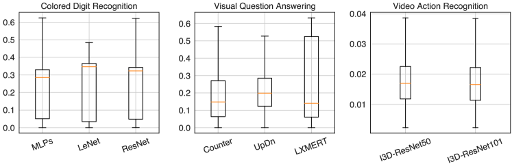
Figure 2. Jensen–Shannon Divergence values computed from two distributions: the label distribution with respect to the biased modality (i.e.,color for colored digit recognition, question type for VQA and object for video action recognition) and the model outputted scores of incorrect instances.

4. Modality Bias Reduction

A typical multi-modal classification model can be abstracted into three consecutive stages: a) multi-modal input representation; b) multi-modal fusion and c) classifier. The first stage takes as inputs the raw multi-modal data and outputs the embedded features. Thereafter, the features are fused with delicately designed manners yet not limited to simple concatenation (Noori et al., 2020) and addition (Zhuang et al., 2020). Finally, a cross entropy loss function is employed to map the fused features to one or a few classes. It is worth noting that the modality bias problem can be triggered by any of the above three stages. In this work, from a generic view, we aim to tackle this problem based on classifier balancing and design a novel loss function. To this end, our objective becomes the frequent and sparse classes respectively taking broader and tighter feature spans in the final feature space, respectively.

4.1. Formulation Background

Following the prevalent formulation, we consider the multi-modal classification as a multi-class single-/multi-label classification problem. That is, for input data with multiple modalities $M=\{M_{1},M_{2},...M_{n}\}$, the objective function is given by:

(1) $$\hat{y}=\mathop{\arg\max}_{y\in\Omega}p(y|M_{1},M_{2},...M_{n};\Theta),$$

where $\Omega$ and $\Theta$ denote the available class set and the model parameters, respectively.

SoftMax. The most popular cross entropy loss function (we tag it as SoftMax) is then formulated as:

(2) $$L_{softmax} =\sum_{i=1}^{|\Omega|}-y_{i}\log p_{i}$$

$$=\sum_{i=1}^{|\Omega|}-y_{i}\log\frac{\exp(\mathbf{W}_{i}^{T}\mathbf{x})}{\sum_{j=1}^{|\Omega|}\exp(\mathbf{W}_{j}^{T}\mathbf{x})},$$

where $\mathbf{W}$ and $\mathbf{x}$ denote the weight matrix and feature vector directly adjacent to the class prediction, respectively. Note that for single-label classification, there is only one label $y_{i}$ equals 1 while others in the label vector $\bf{y}$ are kept as 0. When it comes to multi-label scenario, the involved ground-truth can be smoothed within the range of $(0,1]$. Besides, we remove the bias vector for simplicity as we found it contributes little to the final model performance.

NSL. Recently, some studies have been dedicated to challenging the domination of traditional SoftMax loss function for classification tasks (Deng et al., 2019; Wang et al., 2018). Among these efforts, switching from Euclidean space to Cosine space has been proven to be an intriguing fashion, which employs $L2$ normalization on both the final features as well as the weight vectors. By removing radial variations, it relieves the need for joint supervision of the norm and angle from the SoftMax loss. To approach this idea, we firstly leverage the $L2$ normalization on weight vector $\mathbf{W}_{i}$ and feature vector $\mathbf{x}$ (Pernici et al., 2019). It is leveraged to ensure the posterior probability to be determined by the angle $\theta_{i}$ between $\mathbf{W}_{i}$ and $\mathbf{x}$, i.e.,$||\mathbf{W}_{i}||_{2}=1$ and $||\mathbf{x}||_{2}=1$ given the condition that $\mathbf{W}_{i}^{T}\mathbf{x}=||\mathbf{W}_{i}||||\mathbf{x}||cos\theta_{i}$. Accordingly, the feature space is converted from the Euclidean space to the Cosine one. We then provide the modified normalized SoftMax loss (NSL) (Wang et al., 2018) as follows,

(3) $$L_{nsl}=\sum_{i=1}^{|\Omega|}-y_{i}\log\frac{\exp{(s\times\cos{\theta_{i}})}}{\sum_{j=1}^{|\Omega|}\exp{(s\times\cos{\theta_{j}})}},$$

where $s$ is a scale factor for more stable computation.

LMCL. In order to achieve a more discriminative classification boundary, LMCL (Wang et al., 2018) introduces a fixed cosine margin to NSL,

(4) $$L_{lmcl}=\sum_{i=1}^{|\Omega|}-y_{i}\log\frac{\exp{s(\cos{\theta_{i}}-m)}}{\sum_{j\neq i}\exp{s\times\cos{\theta_{j}}}+\exp{s(\cos{\theta_{i}}-m)}},$$

where $m$ implies the fixed cosine margin. Compared to the Euclidean space, the Cosine space is relatively easy to manipulate, as the margin range reduces from $(-\infty,+\infty)$ to $[-1,1]$.

Regarding the implementation, we found that applying a fixed cosine margin cannot obtain satisfactory results. The key reason is that label distribution is highly skewed given the biased modality, resulting in the incapability of learning a sufficient representation with a fixed margin in the Cosine space. In the next subsection, we will introduce a more sophisticated adapted margin cosine loss to overcome this issue.

4.2. Proposed Method

The results in our experiments (see Sect. 6.2) explicitly demonstrate that a fixed cosine margin yields limited improvements or even degrades the model performance. Based upon this observation, we argue that an adapted cosine margin is more favorable for tackling the bias problem in multi-modal classification. In view of this, a new loss function named Multi-Modal De-Bias (MMDB) is defined as:

(5) $$\left\{\begin{aligned} &L_{MMDB}=\sum_{i=1}^{|\Omega|}-y_{i}\log\frac{\exp{s(\cos{\theta_{i}}-m_{i})}}{\sum_{j=1}^{||\Omega||}\exp{s(\cos{\theta_{j}}-m_{j})}},\\ &m_{i}=1-\bar{m}_{i},\\ &\bar{m}_{i}=\frac{n_{i}^{k}+\epsilon}{\sum_{j=1}^{|\Omega|}n_{j}^{k}+\epsilon},\end{aligned}\right.$$

where $m_{i}$ is the adapted margin for label $i$ which is estimated solely on the biased modality, $n_{i}^{k}$ denotes the number of label $i$ under the biased modality $b_{k}$ (e.g.,color for colored digit recognition) in the training set, $\epsilon=1e-6$ is a hyper-parameter for avoiding computational overflow. The underlying intuition is that, for the current given biased modality, the frequent classes span broader in the Cosine space (smaller margin), while sparse classes span tighter (larger margin). In other words, frequent classes imply more training samples, which require a broader feature space to sufficiently cover these classes. In contrast, a tighter feature space is acceptable for sparse classes as the number of training samples is much smaller. This setting enables the models to place a better margin in the Cosine feature space.

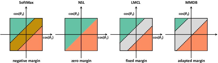
Figure 3. The visual comparison of decision boundary from different loss functions.

Partial derivatives. We further provide the partial derivatives of the weight vector $\mathbf{W}_{i}$ and feature vector $\mathbf{x}$ from our loss function. Let $p_{i}=s(\cos{\theta_{i}}-m_{i})=s(\frac{\mathbf{W}_{i}^{T}}{||\mathbf{W}_{i}||_{2}}\cdot\frac{\mathbf{x}}{||\mathbf{x}||_{2}}-m_{i})$, and $\hat{p}_{i}=\frac{\exp{p_{i}}}{\sum_{j=1}^{|\Omega|}\exp{p_{j}}}$. The partial derivatives are obtained via,

(6) $$\frac{\partial L_{MMDB}}{\partial\mathbf{x}}=\sum_{i=1}^{|\Omega|}(\sum_{j=1}^{|\Omega|}y_{j}\times\hat{p}_{i}-y_{i})\times s\times\frac{||\mathbf{x}||_{2}\mathbf{I}-\mathbf{x}\mathbf{x}^{T}}{||\mathbf{x}||_{2}^{3}}\frac{\mathbf{W}_{i}}{||\mathbf{W}_{i}||_{2}},$$

and

(7) $$\frac{\partial L_{MMDB}}{\partial\mathbf{W}_{i}}=\sum_{i=1}^{|\Omega|}(\sum_{j=1}^{|\Omega|}y_{j}\times\hat{p}_{i}-y_{i})\times s\times\frac{||\mathbf{W}_{i}||_{2}\mathbf{I}-\mathbf{W}_{i}\mathbf{W}_{i}^{T}}{||\mathbf{W}_{i}||_{2}^{3}}\frac{\mathbf{x}}{||\mathbf{x}||_{2}}.$$

Lower bound for s. The scale factor $s$ is critical for the final feature learning. A too small $s$ leads to an insufficient convergence as it limits the feature space span (as we found in our experiments that the loss goes ‘nan’ with a small $s$). In view of this, a lower bound for $s$ should be prescribed. Without loss of generality, let $P_{i}$ denote the expected minimum of the class $i$, the lower bound is defined as,

(8) $$s\geq\frac{\ln(\nicefrac{{1}}{{P_{i}}}-1)}{m_{i}+\nicefrac{{\sum_{j\neq i}m_{j}}}{{(|\Omega|-1}})-2}.$$

The detailed proof is provided in Appendix A.

4.3. Application over Specific Tasks

We apply our MMDB loss function to three tasks according to their distinctive characteristics.

Colored Digit Recognition. As discussed in Section 3, compared to the shape modality, the color serves as the key biased factor in this task. For instance, most 0 digits correspond to the blue color (ref. Fig. 1). In view of this, we compute the margin $\bar{m}_{i}$ with the constraint of colors, namely, $n_{i}^{k}$ is the number of digit $i$ under the color $k$.

Visual Question Answering. Some studies have been conducted on the language prior problem in VQA (Agrawal et al., 2018; Ramakrishnan et al., 2018; Guo et al., 2021a). The language shortcut is deemed as the bias factor, where its expression is the strong link between question type (the first few words in a question) and the textual answer. Motivated by this observation, $n_{i}^{k}$ in Eqn. 5 can be simply estimated by the number of answer $i$ under the question type $k$. As a result, for the given question and its corresponding question type, the frequent answers span broader in the Cosine space (smaller margin) while sparse answers learn tighter feature space (larger margin).

Video Action Recognition. Though actions in videos are expected to be recognized with the temporal information, nevertheless, we find that some of them are easy to be classified with the spatial modality, or more specifically, the objects in static frames. To this end, we leverage the number of action $i$ under the detected object $k$ to compute the $n_{i}^{k}$, which is expected to alleviate the modality bias problem within this task.

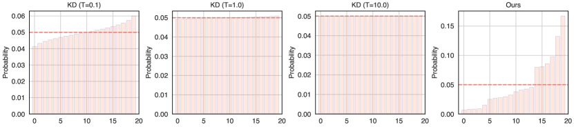
Figure 4. Probability comparison from 20 classes between KD and our method where the probabilities are arranged from small to large. The left three ones respectively denote the KD with temperature 0.1, 1.0 (i.e.,SoftMax) and 10.0. And the right most illustrates the probability yields from our method. The averaged probability from the 20 classes are outlined in red for all cases.

4.4. Comparison with Different Loss Functions

We consider the binary-class scenario for intuitively illustrating the decision boundary from different loss functions. As can be seen from Fig. 3, the decision boundary of the plain SoftMax one can be negative, which is enlarged to be equal to zero of the NSL loss (Wang et al., 2018). The LMLC (Wang et al., 2018) defines a fixed margin for different classes, yet is not suitable in our case for overcoming the modality bias problem. Regarding our MMDB, a sparser class (green one) is mapped to a smaller feature space while a more frequent class (orange one) engages with a larger feature space.

4.5. An Empirical Explanation

To understand why the proposed loss function works, recall that $\mathbf{W}_{i}^{T}\mathbf{x}=||\mathbf{W}_{i}||\times||\mathbf{x}||\times\cos{\theta_{i}}=s\times\cos{\theta_{i}}$, we firstly unfold $L_{MMDB}$ with:

(9) $$L_{MMDB} =\sum_{i=1}^{|\Omega|}-y_{i}\log\frac{\exp{s(\cos{\theta_{i}}-m_{i})}}{\sum_{j=1}^{||\Omega||}\exp{s(\cos{\theta_{j}}-m_{j})}}$$

$$=\sum_{i=1}^{|\Omega|}-y_{i}\log\frac{\exp{(\mathbf{W}_{i}^{T}\mathbf{x}-s\times m_{i})}}{\sum_{j=1}^{||\Omega||}\exp{(\mathbf{W}_{j}^{T}\mathbf{x}-s\times m_{j})}}$$

$$=\sum_{i=1}^{|\Omega|}-y_{i}\log\frac{\nicefrac{{\exp{(\mathbf{W}_{i}^{T}\mathbf{x}})}}{{\exp{(s\times m_{i})}}}}{\sum_{j=1}^{||\Omega||}\nicefrac{{\exp{(\mathbf{W}_{j}^{T}\mathbf{x})}}}{{\exp{(s\times m_{j})}}}}.$$

We then rewrite,

(10) $$T_{i}=\exp{(s\times m_{i})},$$

where we name $T_{i}$ as the temperature for class $i$, which produces,

(11) $$L_{MMDB}=\sum_{i=1}^{|\Omega|}-y_{i}\log\frac{\nicefrac{{\exp{(\mathbf{W}_{i}^{T}\mathbf{x})}}}{{T_{i}}}}{\sum_{j=1}^{||\Omega||}\nicefrac{{\exp{(\mathbf{W}_{j}^{T}\mathbf{x})}}}{{T_{j}}}}.$$

Note that the logits are softened in the well-studied knowledge distillation (KD) domain (Li et al., 2021; Hinton et al., 2015) through,

(12) $$q_{i}=\frac{\exp(\nicefrac{{\mathbf{W}_{i}^{T}\mathbf{x}}}{{T}})}{\sum_{j=1}^{||\Omega||}\exp(\nicefrac{{\mathbf{W}_{j}^{T}\mathbf{x}}}{{T}})},$$

where $T$ denotes the temperature during distilling and $q_{i}$ represents the probability for label $i$. There are two main differences between our method and KD: 1) we move the temperature outside the scope of the exponential function; and 2) the temperature is distinct for different labels. A visual comparison of the produced probabilities is demonstrated in Fig. 4. We can observe that larger temperatures from KD leads to more balanced probabilities, which produces more “informative” labels as argued by (Hinton et al., 2015). However, this may contradict the scenario studied in this paper, as the most “informative” classes to the current target are naturally the ones inducing the modality bias problem. In contrast, our method in Fig. 4 demonstrates a sharp probability distribution, which aids the reduction of this problem to some extent.

5. Experimental Setting

We conducted extensive experiments on the aforementioned three multi-modal classification tasks, to validate the effectiveness of the proposed method. In particular, the experiments are mainly performed to answer the following research questions:

• RQ1: Can the proposed multi-modal de-bias loss function method overcome the modality bias problem?

• RQ2: How do fixed margins in Eqn. 4 and the scale in Eqn. 5 affect the final model performance?

• RQ3: Why does the proposed method outperform the baselines?

To answer these questions, we firstly present the experimental setup for the three tasks.

5.1. Colored Digit Recognition

Dataset. Li et al. (Li and Vasconcelos, 2019) firstly introduced the Colored MNIST dataset, where the color for the ten classes is made distinctive from each other. We observed that the training and testing sets still follow an I.I.D property, which is however, deficient to evaluate the modality bias problem. To this end, we proposed to perturb the color assignment for these two sets. In our experiments, we mainly tested the model performance on the newly curated OoD Colored MNIST dataset.

Evaluation Metric. We adopted the standard accuracy metric for this experiment.

Tested Baselines. As the Colored MNIST dataset is relatively simple to address, therefore, a two-layer MLPs, LeNet (LeCun et al., 1998) as well as a slightly cumbersome ResNet18 (He et al., 2016) baselines are utilized. In addition, we also compared with two approaches working on the bias problem, i.e.,Repair (Li and Vasconcelos, 2019) and BiaSwap (Kim et al., 2021). And we ran each method for five times and reported the averaged accuracy.

5.2. Visual Question Answering

Datasets. We justified our proposed method on the two VQA-CP datasets: VQA-CP v2 and VQA-CP v1 (Agrawal et al., 2018), which are widely accepted benchmarks for evaluating the models’ capability to overcome the language prior problem. The VQA-CP v2 and VQA-CP v1 datasets consist of $\sim$122K images, $\sim$658K questions and $\sim$6.6M answers, and $\sim$122K images, $\sim$370K questions and $\sim$3.7M answers, respectively. Moreover, the answer distribution per question type is significantly different between training and testing sets (OoD property). For all the datasets, the answers are divided into three categories: Y/N, Num. and Other.

Evaluation Metric. We adopted the standard metric in VQA for evaluation (Antol et al., 2015). For each predicted answer $a$, the accuracy is computed as,

(13) $$Acc=\text{min}(1,\frac{\#\text{humans that provide answer $a$}}{3}).$$

Note that each question is answered by ten annotators, and this metric takes the human disagreement into consideration (Antol et al., 2015; Goyal et al., 2017).

Tested Baselines. Inherited from previous attention-based VQA models, Counter (Zhang et al., 2018) introduces a counting module to enable robust counting from object proposals. UpDn (Anderson et al., 2018) firstly leverages the pre-trained object detection frameworks to obtain salient object features for high-level reasoning. It then employs a simple attention network to focus on the most important objects which are highly related with the given question. In addition, the strong baseline LXMERT (Tan and Bansal, 2019) is built upon the Transformer encoders to learn the connections between vision and language. It is pre-trained with diverse pre-training tasks on several large-scale datasets of image and sentence pairs and achieves significant performance improvement on downstream tasks including VQA.

5.3. Video Action Recognition

Dataset. For this multi-modal task, we performed experiments on the widely exploited Kinetics-400 and Kinetics-700 datasets (Kay et al., 2017). In general, there are 400 and 700 action classes in these two datasets, respectively, with 400–1,150 clips for each action. And each clip is from a unique video. Each clip lasts around 10s and corresponds to a total number of 306,245 and 647,907 videos for the two datasets, respectively.

Evaluation Metric. Followed previous video action recognition methods (Chen et al., 2021), we adopted the clip-level accuracy, e.g.,Precision@1 and Precision@5 as the evaluation metrics.

Tested Baselines. We employed our loss function over the I3D (Carreira and Zisserman, 2017) network with two backbones - ResNet50 and ResNet101. As demonstrated in  (Chen et al., 2021), this simple method performs on par with or even outperforms many recent methods that are claimed to be better. Due to the resource limitation, we reduced the number of frames per video and the batch size for both methods to 8 and 16, respectively, while kept other settings the same as the released code. In addition, we also studied the effectiveness of our loss function on two recently developed strong baselines - TimeSformer (Bertasius et al., 2021) and ViViT (Arnab et al., 2021).

It is worth noting that for all the baselines with respect to the above three tasks, we simply replaced the cross entropy loss with our MMDB and did NOT change any other settings, such as embedding size, learning rate, optimizer, and batch size. Therefore, our method will not introduce any incremental cost into those baseline models during the testing stage, since the inference of both our method and the baselines are identical.

6. Experimental Results

6.1. Overall Performance Comparison (RQ1)

6.1.1. Colored Digit Recognition.

We applied our method to three baselines: MLPs, LeNet and ResNet18 and report the results in Fig. 5. The observations are as follows:

• All the three methods can achieve certain performance improvements over the plain baselines. Our method, i.e.,MMDB can outperform Repair (Li and Vasconcelos, 2019) and BiaSwap (Kim et al., 2021) with significant gains on all the three baselines.

• Our method can significantly enhance the baselines with large performance margins. Specifically, the improved accuracy on MLPs, LeNet and ResNet18 are around 14%, 12% and 25%, respectively. This demonstrates that the modality bias problem is reduced by our MMDB.

• Compared to the baselines, more stable error bar can be seen for MMDB. It shows that our method is more robust over multiple runs, which serves as another merit.

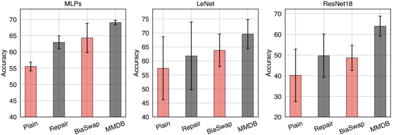
Figure 5. Performance comparison between our MMDB and three baselines on the colored digit recognition task. The error bars are also shown.

Table 4. Accuracy comparisons with respect to different answer categories over the VQA-CP v2 dataset. Regarding the method group, the top group denotes plain approaches, the middle group represents methods directly applied on the UpDn baseline, and the approaches from the last group are with our loss function. ‘$-$’ and ‘${\dagger}$’ denote the numbers are unavailable and our implementation, respectively. The best performance in current splits is highlighted in bold.

Method	VQA-CP v2 test
	Y/N	Num.	Other	All
NMN (Andreas et al., 2016)	38.94	11.92	25.72	27.47
MCB (Fukui et al., 2016)	41.01	11.96	40.57	36.33
Counter† (Zhang et al., 2018)	41.01	12.98	42.69	37.67
UpDn (Anderson et al., 2018)	42.27	11.93	46.05	39.74
UpDn† (Anderson et al., 2018)	49.78	14.07	43.42	40.79
LXMERT† (Tan and Bansal, 2019)	46.70	27.14	61.20	51.78
GVQA (Agrawal et al., 2018)	57.99	13.68	22.14	31.30
AdvReg (Ramakrishnan et al., 2018)	65.49	15.48	35.48	41.17
Rubi (Cadène et al., 2019)	68.65	20.28	43.18	47.11
LMH (Clark et al., 2019)	-	-	-	52.05
LMH† (Clark et al., 2019)	70.29	44.10	44.86	52.15
SCR (Wu and Mooney, 2019)	72.36	10.93	48.02	49.45
VGQE (Johnson et al., 2017b)	66.35	27.08	46.77	50.11
CSS (Chen et al., 2020)	43.96	12.78	47.48	41.16
Decomp-LR (Jing et al., 2020)	70.99	18.72	45.57	48.87
Counter+Ours	61.00	53.22	43.17	49.90
UpDn+Ours	72.47	53.81	45.58	54.67
LXMERT+Ours	91.37	65.55	62.61	71.44

Table 5. Accuracy comparisons with respect to different answer categories over the VQA-CP v1 dataset. ‘${\dagger}$’ denotes our implementation. The best performance in current splits is highlighted in bold.

Method	VQA-CP v1 test
	Y/N	Num.	Other	All
NMN (Andreas et al., 2016)	38.85	11.23	27.88	29.64
MCB (Fukui et al., 2016)	37.96	11.80	39.90	34.39
Counter† (Zhang et al., 2018)	40.93	12.87	42.72	37.08
UpDn† (Anderson et al., 2018)	43.76	12.49	42.57	38.02
GVQA (Agrawal et al., 2018)	64.72	11.87	24.86	39.23
AdvReg (Ramakrishnan et al., 2018)	74.16	12.44	25.32	43.43
LMH† (Clark et al., 2019)	76.61	29.05	43.38	54.76
LXMERT (Tan and Bansal, 2019)	54.08	25.05	62.72	52.82
Counter+Ours	72.01	49.28	42.60	55.92
UpDn+Ours	91.17	41.34	39.38	61.20
LXMERT+Ours	92.67	61.37	64.04	75.47

Table 6. Performance Comparison on the OoD version of the Kinetics-400 and Kinetics-700 datasets.

Dataset	Method	Baseline		MMDB
		Precision@1	Precision@5	Precision@1	Precision@5
Kinetics-400	I3D-ResNet50 (Carreira and Zisserman, 2017)	52.20	80.47	54.57	81.10
	I3D-ResNet101 (Carreira and Zisserman, 2017)	53.64	81.54	55.66	81.82
	TimeSformer (Bertasius et al., 2021)	72.01	90.75	73.65	91.36
	ViViT (Arnab et al., 2021)	75.24	93.25	75.39	93.50
Kinetics-700	I3D-ResNet50 (Carreira and Zisserman, 2017)	37.21	66.05	38.95	67.47
	I3D-ResNet101 (Carreira and Zisserman, 2017)	30.52	59.20	34.60	62.25
	TimeSformer (Bertasius et al., 2021)	61.33	83.90	65.65	86.28
	ViViT (Arnab et al., 2021)	72.00	91.41	74.83	92.01

6.1.2. Visual Question Answering.

The experimental results on VQA-CP v2 and VQA-CP v1 are illustrated in Table 4 and Table 5, respectively. The main observations from these two tables are listed below:

• In general, the methods in the middle group of Table 4 (specially designed to overcome the language bias problem) often outperform previous strong baselines (e.g.,FiLM (Perez et al., 2018)). This result is intuitive as conventional approaches may introduce biases to model learning.

• Our method obtains the best results on the two benchmark datasets. With the help of the recent strong baseline LXMERT, it surprisingly achieves a new state-of-the-art on these two benchmarks.

• For all the three baselines, i.e.,Counter, UpDn and LXMERT, when equppied with our MMDB loss function, a drastic performance improvement (15% on average) can be observed. For example, on the VQA-CP v2 dataset, LXMERT+Ours achieves an absolute performance gain of 19.66% on the All answer category; and on the VQA-CP v1 dataset, UpDn+Ours outperforms the baseline UpDn with 23.18% on the All category.

• Compared with other methods whose backbone model is also UpDn on the VQA-CP v2 dataset, our method (UpDn+Ours) still surpasses them by a large margin, especially for the three newly developed approaches VGQE, CSS and Decomp-LR.

6.1.3. Video Action Recognition.

We tested the effectiveness of our method on the I3D network (Carreira and Zisserman, 2017) with two backbones – ResNet50 and ResNet101, TimeSformer (Bertasius et al., 2021) and ViViT (Arnab et al., 2021). From the results in Table 6, it can be seen that our method can boost the backbone with a significant improvement, especially for the Precision@1, the improvements are 2.27% and 2.02% for ResNet50 and ResNet101 on the Kinetics-400 dataset, respectively.

Table 7. Effectiveness validation of the proposed loss function on three multi-modal learning tasks. For methods on Kenetics-400, we reported the Precision@1 metric.

Method	Margin	Colored MNIST			VQA-CP v2			Kenetics-400
		MLPs	LeNet	ResNet	Counter	UpDn	LXMERT	I3D-ResNet50	I3D-ResNet101
Baseline	-	55.55	57.39	40.19	37.67	40.79	51.78	52.20	53.64
NSL	-	56.48	55.93	48.70	49.08	40.97	58.06	53.95	55.45
Fixed Margin	0.1	58.55	60.06	54.84	30.12	39.42	56.56	52.15	47.32
	0.3	19.92	58.18	52.73	27.70	37.75	55.05	46.54	46.78
	0.5	9.80	9.80	51.27	13.07	36.60	53.81	43.36	44.18
	0.7	9.80	9.80	53.80	11.41	35.83	53.19	42.71	43.31
	0.9	9.80	9.80	56.05	3.12	35.68	52.62	43.19	43.33
Adapted Margin	adaptive	68.05	69.59	64.00	49.90	54.67	71.42	54.57	55.66

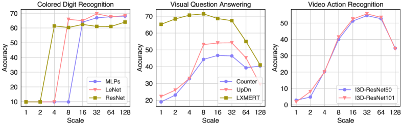
Figure 6. Performance change with respect to the scale $s$ in Eqn. 5.

6.2. Ablation Study (RQ2)

For a deeper understanding of our MMDB, we further provided detailed ablation studies over these three tasks.

Fixed margin results. As mentioned in section 4, models with a fixed margin perform unsatisfactorily when compared with our adaptive ones. The results are shown in Table 7 and we have the following observations:

• When using the $L2$ normalization on both the weight vector and the feature vector, the de facto NSL function, the results are inconsistent amongst different methods. For example, the Counter in VQA with NSL surpasses the baseline with 11.41%, while LeNet in colored digit recognition with NSL even causes a little bit deterioration of the performance.

• We also tested the fixed margin to yield effective feature discrimination, where the margins are tuned from 0.1 to 0.9 with a step size of 0.2. However, the results are not favorable (the improvement is limited), which validates the evidence that a fixed margin is not suitable for overcoming the modality bias problem. By contrast, when replacing the fixed margin with our adaptive one, the model can achieve significant performance improvement, which additionally proves the superiority of MMDB.

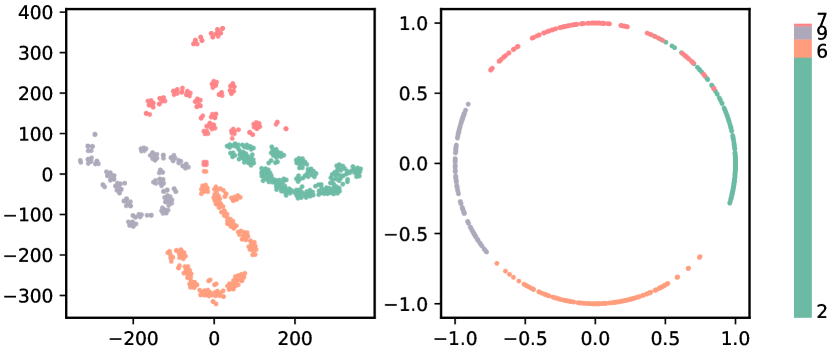
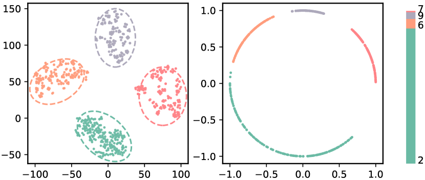
Figure 7. Digit feature manifold embedding of red color for the colored digit recognition task.

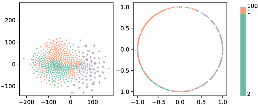
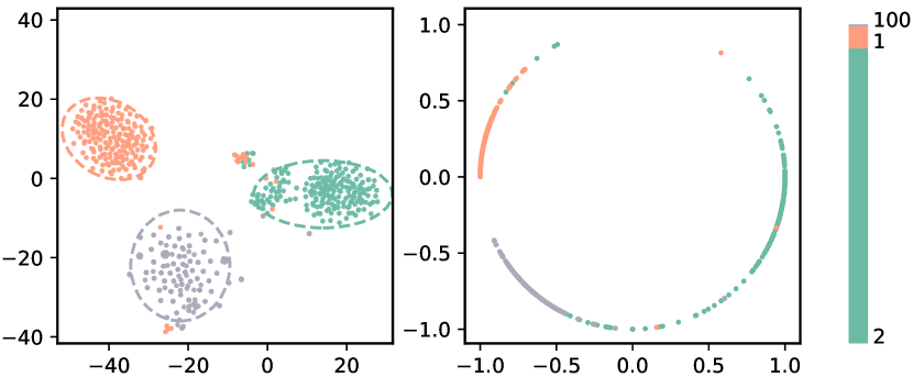
Figure 8. Answer feature manifold embedding of how many question type for the VQA task.

Scale influence. We tuned the scale in Eqn. 5 from 1 to 128 with a step size of $2^{n}$ for all the eight methods. From the results in Fig. 6, we found that a too small scale is insufficient for learning the feature space, resulting in unsatisfactory results. In addition, when the scale becomes large, the performance will saturate or even drop to some degrees.

6.3. Case Study (RQ3)

In this subsection, we use case studies analyze the reasons why the proposed method works from the following two aspects: feature embedding separation and better attention maps.

Feature manifold embedding. Since the key motivation of the proposed method is to achieve the goal that frequent and sparse labels under certain biased modality span broader and tighter in the final feature space, respectively, we therefore visualized the learned features and displayed the results on Fig. 8 and Fig. 8. In particular, we leveraged two tasks - colored digit recognition and VQA for illustration. For the former task, the color modality is restricted to red, and the language modality in the later task is expressed through the how many question type. For the two instances, the top two sub-figures are the feature embedding on the Euclidean and Cosine space from the baseline, while results from our method are summarized in the bottom two sub-figures. It is evident to us that 1) in the Euclidean space, the features are often irregular and even entangled with each other of baselines. Nevertheless, our method can separate these labels with clear boundaries. In addition, when it refers to the Cosine space, frequent labels (e.g.,digit 2 for colored digit recognition and answer 2 for VQA) span much broader than sparse ones, yet this property cannot be observed by the baseline.

Attention maps in VQA. Finally, we showcased two successful cases of our method and illustrated them in Fig. 9. Regarding the first case, as the answer 2 takes large proportion under the question type how many in the training set, the baseline model thus yields an answer 2 to this question. In contrast, our MMDB corrects this mistake, producing a more reasonable attention map (focusing solely on one car). As for the second case, the baseline model wrongly predicts the answer tennis mainly attribute to tennis being more frequent under the question type what sport in the training set. Besides, too much attention has been paid to less relevant regions, which is another reason leading to the incorrect answer. On the contrary, our MMDB can guide the model to emphasize more on the target object - glove, resulting in the correct answer baseball.

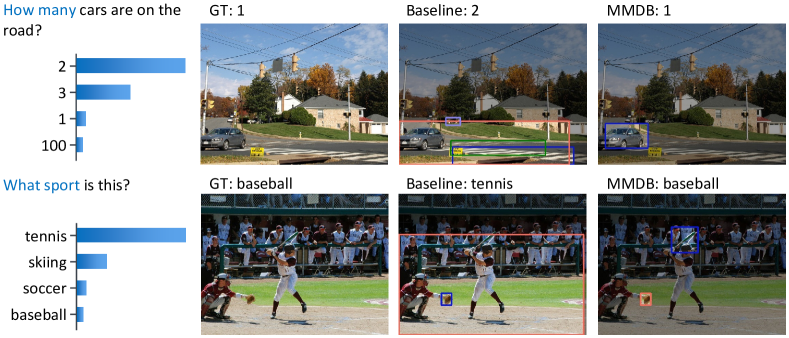
Figure 9. Visualization of the baselines method (UpDn) with and without our proposed loss function MMDB. The key answer distributions under the question’s corresponding question type are illustrated on the leftmost column. The ground-truth is displayed on the second column, followed by the attention maps produced by the baseline and ours on the last two columns.

7. Conclusion and Discussion

In this work, we have systematically studied the modality bias problem in the context of multi-modal classification. To begin with, we construct several Our-of-Distribution datasets as test beds for its evaluation. Thereafter, a multi-modal de-bias loss is designed to discriminate the labels via properly characterizing the feature space. Concretely, for the given biased modality, the frequent and sparse labels with respect to the corresponding modality factors are learned to span broader and tighter in the Cosine space, respectively. Extensive experiments over four benchmarks regarding three multi-modal tasks have been conducted, which validates the effectiveness of the proposed loss function on ten baselines.

Enlightened by the most recent studies on the tackling of the long-tail problem (Zhang et al., 2021; Lee et al., 2021), which rely on the training set statistic to work, our method also leverages such prior to approach the modality bias problem. Though obtained significant performance improvements, this restriction positions our MMDB at the cost of explicit bias conjecture beforehand, limiting its generalization capability across datasets. One potential solution is to discover the biased modalities without presumptions or labels (Li and Xu, 2021b) in the first step. After that, our method can be seamlessly combined with such techniques to perform with the ease of the prior pain. It is worth mentioning that this work does not present an advanced model for pursuing the SOTA results in multi-modal learning. We instead expect that, with this de-bias loss function, future research can focus more on the enhancement of the multi-modal understanding while with less affect of the modality bias.

With the recognition of this problem in multi-modal classification, exploring its associated expression for generation tasks will open an interesting door to increase the output diversity. In addition, tackling the modality bias problem from the other two stages, i.e.,multi-modal representation and fusion, demands our further research attention as well.

Appendix A Proof for the Scaling Factor s

Without loss of generality, let $P_{i}$ denotes the expected minimum of the class $i$. In the ideal formulation, the $\theta_{i}$ between label $i$ and weight vector $\mathbf{W}_{i}$ should be $0$, while that for others labels should be $180$. We then have:

$$\frac{\exp{s(1-m_{i})}}{\sum_{j\neq i}\exp{s(-1-m_{j})}+\exp{s(1-m_{i})}} \geq P_{i},$$

$$1+\frac{\sum_{j\neq i}\exp{s(-1-m_{j})}}{\exp{s(1-m_{i})}} \leq\frac{1}{P_{i}},$$

$$1+\frac{\sum_{j\neq i}\exp{s(m_{j})}}{\exp{s(2-m_{i})}} \leq\frac{1}{P_{i}}.$$

On the basis of Jensen’s inequality,

$$\sum_{j\neq i}\exp{s(m_{j})} =\frac{|\Omega|-1}{|\Omega|-1}\sum_{j\neq i}\exp{s(m_{j})},$$

$$\geq(|\Omega|-1)\exp{s(\frac{\sum_{j\neq i}m_{j}}{|\Omega|-1})}.$$

Accordingly, we obtain,

$$1+\frac{(|\Omega|-1)\exp{s(\nicefrac{{\sum_{j\neq i}m_{j}}}{{(|\Omega|-1}}))}}{\exp{s(2-m_{i})}} \leq\frac{1}{P_{i}},$$

$$\exp{s(\frac{\sum_{j\neq i}m_{j}}{|\Omega|-1}+m_{i}-2)} \leq\frac{1}{P_{i}}-1.$$

Finally, we have,

(14) $$s\geq\frac{\ln(\nicefrac{{1}}{{P_{i}}}-1)}{m_{i}+\nicefrac{{\sum_{j\neq i}m_{j}}}{{(|\Omega|-1)}}-2}.$$

- (1)
- Agrawal et al. (2018) Aishwarya Agrawal, Dhruv Batra, Devi Parikh, and Aniruddha Kembhavi. 2018. Don’t Just Assume; Look and Answer: Overcoming Priors for Visual Question Answering. In IEEE Conference on Computer Vision and Pattern Recognition. IEEE, 4971–4980.
- Anderson et al. (2018) Peter Anderson, Xiaodong He, Chris Buehler, Damien Teney, Mark Johnson, Stephen Gould, and Lei Zhang. 2018. Bottom-Up and Top-Down Attention for Image Captioning and Visual Question Answering. In IEEE Conference on Computer Vision and Pattern Recognition. IEEE, 6077–6086.
- Andreas et al. (2016) Jacob Andreas, Marcus Rohrbach, Trevor Darrell, and Dan Klein. 2016. Neural Module Networks. In IEEE Conference on Computer Vision and Pattern Recognition. IEEE, 39–48.
- Antol et al. (2015) Stanislaw Antol, Aishwarya Agrawal, Jiasen Lu, Margaret Mitchell, Dhruv Batra, C. Lawrence Zitnick, and Devi Parikh. 2015. VQA: Visual Question Answering. In IEEE International Conference on Computer Vision. IEEE, 2425–2433.
- Arnab et al. (2021) Anurag Arnab, Mostafa Dehghani, Georg Heigold, Chen Sun, Mario Lucic, and Cordelia Schmid. 2021. ViViT: A Video Vision Transformer. In International Conference on Computer Vision. IEEE, 6816–6826.
- Bai et al. (2021a) Haoyue Bai, Rui Sun, Lanqing Hong, Fengwei Zhou, Nanyang Ye, Han-Jia Ye, S.-H. Gary Chan, and Zhenguo Li. 2021a. DecAug: Out-of-Distribution Generalization via Decomposed Feature Representation and Semantic Augmentation. In AAAI Conference on Artificial Intelligence. AAAI, 6705–6713.
- Bai et al. (2021b) Haoyue Bai, Fengwei Zhou, Lanqing Hong, Nanyang Ye, S-H Gary Chan, and Zhenguo Li. 2021b. NAS-OoD: Neural Architecture Search for Out-of-Distribution Generalization. In IEEE/CVF International Conference on Computer Vision. IEEE, 8320–8329.
- Bertasius et al. (2021) Gedas Bertasius, Heng Wang, and Lorenzo Torresani. 2021. Is Space-Time Attention All You Need for Video Understanding?. In International Conference on Machine Learning. PMLR, 813–824.
- Cadène et al. (2019) Rémi Cadène, Corentin Dancette, Hedi Ben-younes, Matthieu Cord, and Devi Parikh. 2019. RUBi: Reducing Unimodal Biases for Visual Question Answering. In Advances in Neural Information Processing Systems. MIT, 839–850.
- Caliskan et al. (2017) Aylin Caliskan, Joanna J Bryson, and Arvind Narayanan. 2017. Semantics Derived Automatically from Language Corpora Contain Human-like Biases. Science 356, 6334 (2017), 183–186.
- Carreira and Zisserman (2017) João Carreira and Andrew Zisserman. 2017. Quo Vadis, Action Recognition? A New Model and the Kinetics Dataset. In IEEE Conference on Computer Vision and Pattern Recognition. IEEE, 4724–4733.
- Chen et al. (2021) Chun-Fu (Richard) Chen, Rameswar Panda, Kandan Ramakrishnan, Rogério Feris, John Cohn, Aude Oliva, and Quanfu Fan. 2021. Deep Analysis of CNN-Based Spatio-Temporal Representations for Action Recognition. In IEEE Conference on Computer Vision and Pattern Recognition. IEEE, 6165–6175.
- Chen et al. (2020) Long Chen, Xin Yan, Jun Xiao, Hanwang Zhang, Shiliang Pu, and Yueting Zhuang. 2020. Counterfactual Samples Synthesizing for Robust Visual Question Answering. In IEEE/CVF Conference on Computer Vision and Pattern Recognition. IEEE, 10797–10806.
- Chen and Joo (2021) Yunliang Chen and Jungseock Joo. 2021. Understanding and Mitigating Annotation Bias in Facial Expression Recognition. In IEEE/CVF International Conference on Computer Vision. IEEE, 14980–14991.
- Cheng et al. (2021) Lu Cheng, Ahmadreza Mosallanezhad, Yasin N. Silva, Deborah L. Hall, and Huan Liu. 2021. Mitigating Bias in Session-based Cyberbullying Detection: A Non-Compromising Approach. In Annual Meeting of the Association for Computational Linguistics and International Joint Conference on Natural Language Processing. ACL, 2158–2168.
- Clark et al. (2019) Christopher Clark, Mark Yatskar, and Luke Zettlemoyer. 2019. Don’t Take the Easy Way Out: Ensemble Based Methods for Avoiding Known Dataset Biases. In Conference on Empirical Methods in Natural Language Processing and International Joint Conference on Natural Language Processing. ACL, 4067–4080.
- Deng et al. (2019) Jiankang Deng, Jia Guo, Niannan Xue, and Stefanos Zafeiriou. 2019. ArcFace: Additive Angular Margin Loss for Deep Face Recognition. In IEEE Conference on Computer Vision and Pattern Recognition. IEEE, 4690–4699.
- Dixon et al. (2018) Lucas Dixon, John Li, Jeffrey Sorensen, Nithum Thain, and Lucy Vasserman. 2018. Measuring and Mitigating Unintended Bias in Text Classification. In AAAI/ACM Conference on AI, Ethics, and Society. ACM, 67–73.
- Dou et al. (2019) Qi Dou, Daniel Coelho de Castro, Konstantinos Kamnitsas, and Ben Glocker. 2019. Domain Generalization via Model-Agnostic Learning of Semantic Features. In Advances in Neural Information Processing Systems. MIT, 6447–6458.
- Engstrom et al. (2020) Logan Engstrom, Andrew Ilyas, Shibani Santurkar, Dimitris Tsipras, Jacob Steinhardt, and Aleksander Madry. 2020. Identifying Statistical Bias in Dataset Replication. In International Conference on Machine Learning. PMLR, 2922–2932.
- Fukui et al. (2016) Akira Fukui, Dong Huk Park, Daylen Yang, Anna Rohrbach, Trevor Darrell, and Marcus Rohrbach. 2016. Multimodal Compact Bilinear Pooling for Visual Question Answering and Visual Grounding. In Conference on Empirical Methods in Natural Language Processing. ACL, 457–468.
- Gat et al. (2020) Itai Gat, Idan Schwartz, Alexander G. Schwing, and Tamir Hazan. 2020. Removing Bias in Multi-modal Classifiers: Regularization by Maximizing Functional Entropies. In Advances in Neural Information Processing Systems. MIT.
- Gong et al. (2021) Sixue Gong, Xiaoming Liu, and Anil K. Jain. 2021. Mitigating Face Recognition Bias via Group Adaptive Classifier. In IEEE Conference on Computer Vision and Pattern Recognition. IEEE, 3414–3424.
- Goyal et al. (2017) Yash Goyal, Tejas Khot, Douglas Summers-Stay, Dhruv Batra, and Devi Parikh. 2017. Making the V in VQA Matter: Elevating the Role of Image Understanding in Visual Question Answering. In IEEE Conference on Computer Vision and Pattern Recognition. IEEE, 6325–6334.
- Guo et al. (2019) Yangyang Guo, Zhiyong Cheng, Liqiang Nie, Yibing Liu, Yinglong Wang, and Mohan S. Kankanhalli. 2019. Quantifying and Alleviating the Language Prior Problem in Visual Question Answering. In International ACM SIGIR Conference on Research and Development in Information Retrieval. ACM, 75–84.
- Guo et al. (2021a) Yangyang Guo, Liqiang Nie, Zhiyong Cheng, Feng Ji, Ji Zhang, and Alberto Del Bimbo. 2021a. AdaVQA: Overcoming Language Priors with Adapted Margin Cosine Loss. In International Joint Conference on Artificial Intelligence. ijcai.org, 708–714.
- Guo et al. (2021b) Yangyang Guo, Liqiang Nie, Zhiyong Cheng, Qi Tian, and Min Zhang. 2021b. Loss Re-scaling VQA: Revisiting the Language Prior Problem from A Class-imbalance View. TIP.
- Hama et al. (2021) Kenta Hama, Takashi Matsubara, Kuniaki Uehara, and Jianfei Cai. 2021. Exploring Uncertainty Measures for Image-caption Embedding-and-retrieval Task. ACM Trans. Multim. Comput. Commun. Appl. 17, 2 (2021), 46:1–46:19.
- He et al. (2016) Kaiming He, Xiangyu Zhang, Shaoqing Ren, and Jian Sun. 2016. Deep Residual Learning for Image Recognition. In IEEE Conference on Computer Vision and Pattern Recognition. IEEE, 770–778.
- Hendrycks et al. (2021) Dan Hendrycks, Steven Basart, Norman Mu, Saurav Kadavath, Frank Wang, Evan Dorundo, Rahul Desai, Tyler Zhu, Samyak Parajuli, Mike Guo, et al. 2021. The Many Faces of Robustness: A Critical Analysis of Out-of-Distribution Generalization. In IEEE/CVF International Conference on Computer Vision. IEEE, 8340–8349.
- Hendrycks et al. (2019) Dan Hendrycks, Kimin Lee, and Mantas Mazeika. 2019. Using Pre-Training Can Improve Model Robustness and Uncertainty. In International Conference on Machine Learning. PMLR, 2712–2721.
- Hinton et al. (2015) Geoffrey E. Hinton, Oriol Vinyals, and Jeffrey Dean. 2015. Distilling the Knowledge in a Neural Network. CoRR abs/1503.02531 (2015).
- Huang and Belongie (2017) Xun Huang and Serge J. Belongie. 2017. Arbitrary Style Transfer in Real-Time with Adaptive Instance Normalization. In IEEE International Conference on Computer Vision. IEEE, 1510–1519.
- Jing et al. (2020) Chenchen Jing, Yuwei Wu, Xiaoxun Zhang, Yunde Jia, and Qi Wu. 2020. Overcoming Language Priors in VQA via Decomposed Linguistic Representations. In AAAI Conference on Artificial Intelligence. AAAI, 11181–11188.
- Johnson et al. (2017a) Justin Johnson, Bharath Hariharan, Laurens van der Maaten, Li Fei-Fei, C. Lawrence Zitnick, and Ross B. Girshick. 2017a. CLEVR: A Diagnostic Dataset for Compositional Language and Elementary Visual Reasoning. In IEEE Conference on Computer Vision and Pattern Recognition. IEEE, 1988–1997.
- Johnson et al. (2017b) Justin Johnson, Bharath Hariharan, Laurens van der Maaten, Li Fei-Fei, C. Lawrence Zitnick, and Ross B. Girshick. 2017b. CLEVR: A Diagnostic Dataset for Compositional Language and Elementary Visual Reasoning. In IEEE Conference on Computer Vision and Pattern Recognition. IEEE, 1988–1997.
- Kay et al. (2017) Will Kay, João Carreira, Karen Simonyan, Brian Zhang, Chloe Hillier, Sudheendra Vijayanarasimhan, Fabio Viola, Tim Green, Trevor Back, Paul Natsev, Mustafa Suleyman, and Andrew Zisserman. 2017. The Kinetics Human Action Video Dataset. CoRR abs/1705.06950 (2017).
- Kim et al. (2021) Eungyeup Kim, Jihyeon Lee, and Jaegul Choo. 2021. BiaSwap: Removing Dataset Bias with Bias-Tailored Swapping Augmentation. In International Conference on Computer Vision. IEEE, 14972–14981.
- Kortylewski et al. (2018) Adam Kortylewski, Bernhard Egger, Andreas Schneider, Thomas Gerig, Andreas Morel-Forster, and Thomas Vetter. 2018. Empirically Analyzing the Effect of Dataset Biases on Deep Face Recognition Systems. In IEEE Conference on Computer Vision and Pattern Recognition Workshops. IEEE, 2093–2102.
- LeCun et al. (1998) Yann LeCun, Léon Bottou, Yoshua Bengio, and Patrick Haffner. 1998. Gradient-based Learning Applied to Document Recognition. Proc. IEEE 86, 11 (1998), 2278–2324.
- Lee et al. (2021) Hyuck Lee, Seungjae Shin, and Heeyoung Kim. 2021. ABC: Auxiliary Balanced Classifier for Class-imbalanced Semi-supervised Learning. In Advances in Neural Information Processing. 7082–7094.
- Li et al. (2021) Yanchun Li, Jianglian Cao, Zhetao Li, Sangyoon Oh, and Nobuyoshi Komuro. 2021. Lightweight Single Image Super-resolution with Dense Connection Distillation Network. ACM Trans. Multim. Comput. Commun. Appl. 17, 1s (2021), 1–17.
- Li and Vasconcelos (2019) Yi Li and Nuno Vasconcelos. 2019. REPAIR: Removing Representation Bias by Dataset Resampling. In IEEE Conference on Computer Vision and Pattern Recognition. IEEE, 9572–9581.
- Li and Xu (2021a) Zhiheng Li and Chenliang Xu. 2021a. Discover the Unknown Biased Attribute of An Image Classifier. In IEEE/CVF International Conference on Computer Vision. IEEE.
- Li and Xu (2021b) Zhiheng Li and Chenliang Xu. 2021b. Discover the Unknown Biased Attribute of an Image Classifier. In International Conference on Computer Vision. IEEE, 14950–14959.
- Lu et al. (2019) Boyu Lu, Jun-Cheng Chen, Carlos Domingo Castillo, and Rama Chellappa. 2019. An Experimental Evaluation of Covariates Effects on Unconstrained Face Verification. IEEE Trans. Biom. Behav. Identity Sci. 1, 1 (2019), 42–55.
- Noori et al. (2020) Farzan Majeed Noori, Michael Riegler, Md. Zia Uddin, and Jim Tørresen. 2020. Human Activity Recognition from Multiple Sensors Data Using Multi-fusion Representations and CNNs. ACM Trans. Multim. Comput. Commun. Appl. 16, 2 (2020), 45:1–45:19.
- Park et al. (2018) Ji Ho Park, Jamin Shin, and Pascale Fung. 2018. Reducing Gender Bias in Abusive Language Detection. In Conference on Empirical Methods in Natural Language Processing. ACL, 2799–2804.
- Perez et al. (2022) Ethan Perez, Saffron Huang, H. Francis Song, Trevor Cai, Roman Ring, John Aslanides, Amelia Glaese, Nat McAleese, and Geoffrey Irving. 2022. Red Teaming Language Models with Language Models. In CoRR, Vol. abs/2202.03286.
- Perez et al. (2018) Ethan Perez, Florian Strub, Harm de Vries, Vincent Dumoulin, and Aaron C. Courville. 2018. FiLM: Visual Reasoning with a General Conditioning Layer. In Proceedings of the Thirty-Second AAAI Conference on Artificial Intelligence. AAAI, 3942–3951.
- Pernici et al. (2019) Federico Pernici, Matteo Bruni, Claudio Baecchi, and Alberto Del Bimbo. 2019. Maximally Compact and Separated Features with Regular Polytope Networks. In Computer Vision and Pattern Recognition Workshops. IEEE, 46–53.
- Ramakrishnan et al. (2018) Sainandan Ramakrishnan, Aishwarya Agrawal, and Stefan Lee. 2018. Overcoming Language Priors in Visual Question Answering with Adversarial Regularization. In Advances in Neural Information Processing Systems. MIT, 1548–1558.
- Recht et al. (2019) Benjamin Recht, Rebecca Roelofs, Ludwig Schmidt, and Vaishaal Shankar. 2019. Do ImageNet Classifiers Generalize to ImageNet?. In International Conference on Machine Learning. PMLR, 5389–5400.
- Selvaraju et al. (2019) Ramprasaath Ramasamy Selvaraju, Stefan Lee, Yilin Shen, Hongxia Jin, Shalini Ghosh, Larry P. Heck, Dhruv Batra, and Devi Parikh. 2019. Taking a HINT: Leveraging Explanations to Make Vision and Language Models More Grounded. In IEEE/CVF International Conference on Computer Vision. IEEE, 2591–2600.
- Shah et al. (2020) Deven Shah, H. Andrew Schwartz, and Dirk Hovy. 2020. Predictive Biases in Natural Language Processing Models: A Conceptual Framework and Overview. In Annual Meeting of the Association for Computational Linguistics. ACL, 5248–5264.
- Tan and Bansal (2019) Hao Tan and Mohit Bansal. 2019. LXMERT: Learning Cross-Modality Encoder Representations from Transformers. In Conference on Empirical Methods in Natural Language Processing and International Joint Conference on Natural Language Processing. ACL, 5099–5110.
- Teney et al. (2021) Damien Teney, Ehsan Abbasnejad, and Anton van den Hengel. 2021. Unshuffling Data for Improved Generalization in Visual Question Answering. In IEEE/CVF International Conference on Computer Vision. IEEE, 1417–1427.
- Wang et al. (2019b) Haohan Wang, Zexue He, Zachary C. Lipton, and Eric P. Xing. 2019b. Learning Robust Representations by Projecting Superficial Statistics Out. In International Conference on Learning Representations. OpenReview.net.
- Wang et al. (2018) Hao Wang, Yitong Wang, Zheng Zhou, Xing Ji, Dihong Gong, Jingchao Zhou, Zhifeng Li, and Wei Liu. 2018. CosFace: Large Margin Cosine Loss for Deep Face Recognition. In IEEE Conference on Computer Vision and Pattern Recognition. IEEE, 5265–5274.
- Wang et al. (2019a) Mei Wang, Weihong Deng, Jiani Hu, Xunqiang Tao, and Yaohai Huang. 2019a. Racial Faces in the Wild: Reducing Racial Bias by Information Maximization Adaptation Network. In IEEE/CVF International Conference on Computer Vision. IEEE, 692–702.
- Wang et al. (2019c) Tianlu Wang, Jieyu Zhao, Mark Yatskar, Kai-Wei Chang, and Vicente Ordonez. 2019c. Balanced Datasets Are Not Enough: Estimating and Mitigating Gender Bias in Deep Image Representations. In IEEE/CVF International Conference on Computer Vision. IEEE, 5309–5318.
- Wu and Mooney (2019) Jialin Wu and Raymond J. Mooney. 2019. Self-Critical Reasoning for Robust Visual Question Answering. In Advances in Neural Information Processing Systems. MIT, 8601–8611.
- Zhang et al. (2020) Guanhua Zhang, Bing Bai, Junqi Zhang, Kun Bai, Conghui Zhu, and Tiejun Zhao. 2020. Demographics Should Not Be the Reason of Toxicity: Mitigating Discrimination in Text Classifications with Instance Weighting. In Annual Meeting of the Association for Computational Linguistics. ACL, 4134–4145.
- Zhang et al. (2018) Yan Zhang, Jonathon S. Hare, and Adam Prügel-Bennett. 2018. Learning to Count Objects in Natural Images for Visual Question Answering. In International Conference on Learning Representations. OpenReview.net.
- Zhang et al. (2021) Yongshun Zhang, Xiu-Shen Wei, Boyan Zhou, and Jianxin Wu. 2021. Bag of Tricks for Long-Tailed Visual Recognition with Deep Convolutional Neural Networks. In Thirty-Fifth AAAI Conference on Artificial Intelligence. AAAI, 3447–3455.
- Zhuang et al. (2020) Yueting Zhuang, Dejing Xu, Xin Yan, Wenzhuo Cheng, Zhou Zhao, Shiliang Pu, and Jun Xiao. 2020. Multichannel Attention Refinement for Video Question Answering. ACM Trans. Multim. Comput. Commun. Appl. 16, 1s (2020), 1–23.