PLSSVM: A (multi-)GPGPU-accelerated Least Squares Support Vector Machine

Abstract

Machine learning algorithms must be able to efficiently cope with massive data sets. Therefore, they have to scale well on any modern system and be able to exploit the computing power of accelerators independent of their vendor. In the field of supervised learning, Support Vector Machines (SVMs) are widely used. However, even modern and optimized implementations such as LIBSVM or ThunderSVM do not scale well for large non-trivial dense data sets on cutting-edge hardware: Most SVM implementations are based on Sequential Minimal Optimization, an optimized though inherent sequential algorithm. Hence, they are not well-suited for highly parallel GPUs. Furthermore, we are not aware of a performance portable implementation that supports CPUs and GPUs from different vendors.

We have developed the PLSSVM library to solve both issues. First, we resort to the formulation of the SVM as a least squares problem. Training an SVM then boils down to solving a system of linear equations for which highly parallel algorithms are known. Second, we provide a hardware independent yet efficient implementation: PLSSVM uses different interchangeable backends—OpenMP, CUDA, OpenCL, SYCL—supporting modern hardware from various vendors like NVIDIA, AMD, or Intel on multiple GPUs. PLSSVM can be used as a drop-in replacement for LIBSVM. We observe a speedup on CPUs of up to $10$ compared to LIBSVM and on GPUs of up to $14$ compared to ThunderSVM. Our implementation scales on many-core CPUs with a parallel speedup of $74.7$ on up to $256$ CPU threads and on multiple GPUs with a parallel speedup of $3.71$ on four GPUs.

The code, utility scripts, and documentation are all available on GitHub: https://github.com/SC-SGS/PLSSVM.

I Introduction

The two most common tasks in supervised machine learning are classification and regression. Classification predicts to which set of categories/classes objects or situations belong, while regression estimates the function value of a functional dependency, e.g., a statistical process. Both can be solved using the same algorithms, by matching a function value to two or more discrete classes. Moreover, both share the challenge to scale in the size of the data in order to cope with massive data sets.

In the classification task, the well-known and commonly used Support Vector Machines (SVMs) show competitive performance and have very few parameters to tune. The widely used SVM library LIBSVM [1] has already been cited over $50\,000$ times. A survey conducted by Kaggle in 2017 showed that $26\text{\,}\frac{\mathrm{\char 37\relax}}{}$ of the data mining and machine learning practitioners use SVMs [2]. Examples of current research topics are COVID-19 pandemic predictions [3], automatic COVID-19 lung image classification [4], forecasting of carbon prices [5], face detection [6], or propaganda text recognition [7].

The basic idea of the SVMs was introduced in 1992 by Boser et al. [8] and extended in 1995 by Cortes and Vapnik [9] to the today’s state-of-the-art approach. Based on this approach, Joachims published one of the first SVM libraries SVM^light [10]. Chang and Lin developed LIBSVM [1], which is one of the most widely used SVM libraries today. Both are based on the Sequential Minimal Optimization (SMO) algorithm [11]. Additionally, plenty of research have focused on parallelizing SVMs on multi-core Central Processing Unit (CPU) systems. For example, Fan et al. [12] developed LIBLINEAR as a LIBSVM extension and Zeng et al. [13] described a novel parallel SMO algorithm.

ThunderSVM [14] is a rather new SVM implementation supporting CPUs and NVIDIA Graphics Processing Units (GPUs) using the Compute Unified Device Architecture (CUDA). Additionally, there have been various other attempts to port SVMs efficiently to GPUs, e.g., with CUDA [15, 16, 17], but also using other languages and frameworks such as the Open Computing Language (OpenCL) [18], Python [19, 20], OpenACC [21], or SYCL [22]. However, all approaches mentioned so far are based on SMO, an inherently sequential algorithm, and, therefore, not very well suited for high performance GPU implementations and vast data sets.

Suykens and Vandewalle [23, 24] developed the least squares formulation of the SVM problem. In this formulation, training an SVM is reduced to solving a system of linear equations, a problem for which highly parallel algorithms exist. Suykens et al. improved their Least Squares Support Vector Machine (LS-SVM) further by introducing weights [25] and extending their implementation to also support sparse data structures [26]. Furthermore, they introduced the multi-class classification for LS-SVMs [27]. An exact correlation between SVMs using SMO and LS-SVMs was investigated by Ye and Xiong [28].

Due to the higher parallelization potential of the LS-SVM, we decided to base our Parallel Least Squares Support Vector Machine (PLSSVM) library on the least squares formulation of Suykens and Vandewalle [23]. Our goal is to provide a High Performance Computing (HPC) implementation of a LS-SVM suitable for modern massively parallel heterogeneous hardware.

Do et al. [29, 30] developed an LS-SVM implementation using CUDA to support NVIDIA GPUs. However, they only investigated their implementation on data sets with less than $200$ dimensions. Our PLSSVM implementation can easily cope with data sets having more than $65\,000$ data points with more than $16\,000$ features, as shown in sec:result. Other LS-SVM implementations were developed, e.g., an LS-SVM purely written in Python using PyTorch by Drumond [31].

In this paper, we describe our C++17 PLSSVM library, which efficiently brings SVMs to massively parallel accelerators, and we present and analyze some of our first performance results. We have implemented the basic functionality of the most widely used SVM library, LIBSVM [1], as a drop-in alternative with significant acceleration aided by GPUs. However, sparse data sets, where all but a few feature entries are zero, are treated as if they would represent dense data, i.e., explicitly representing zeros where necessary. As of now, our implementation only supports binary classification.

Our aim is to provide vendor-independent scalable performance for high-end compute nodes. To the best of our knowledge, our PLSSVM library is the first SVM implementation, let alone LS-SVM implementation, that supports multiple backends, in particular OpenMP, CUDA, OpenCL, and SYCL (hipSYCL and DPC++). This allows us to support a broad spectrum of hardware, e.g., GPUs from different vendors like NVIDIA, AMD, and Intel. This distinguishes our approach from most previous implementations, which are restricted to NVIDIA GPUs due to their focus on CUDA. A thorough comparison of the differences and advantages of the individual languages and frameworks for SVMs will be covered in a future work. Furthermore, we support multi-GPU execution for the linear kernel.

This paper is structured as follows: In sec:theory we discuss the basics of SVMs and the transformation into their LS-SVM representation, suitable for highly parallel processing. In sec:impl, we then deduce important implementational details from the LS-SVM equations. In particular, we tackle the problem by solving the resulting equation with the Conjugate Gradients (CG) [32] algorithm and a parallel matrix assembly. In sec:result, we examine our achieved speedup factors, while maintaining accuracies on par with the SMO approaches: up to $10$ for LIBSVM on the CPU and up to $14$ compared to ThunderSVM on a single GPU. Additionally, we investigate the runtime characteristics of the individual components of our library as well as the influence of epsilon (the relative residual used in the CG algorithm) on the runtime and accuracy, and finally we demonstrate that our approach is scalable with a parallel speedup of up to $74.7$ on a many-core CPU with $256$ threads and on four NVIDIA A100 GPUs with a parallel speedup of $3.71$. sec:conclusion concludes this paper with a summary and an outlook on future work.

II Support Vector Machines

In this section, we describe SVMs and their transformation into a least squares problem. The transformation to the LS-SVM is crucial as the state-of-the-art SMO approach is inherently sequential and, therefore, unsuitable for achieving high speedups on massively parallel devices.

II-A Training

To learn an SVM classification model a $d$-dimensional data set $T$ with $m$ data points $\vec{x}_{i}$ and their corresponding labels $y_{i}$ is required for training. Based on $T$, an SVM learns to distinguish between different classes. We assume a binary classification problem and, w.l.o.g., that classes are labeled $y_{i}=\pm 1$. The actual learning process is to find the hyperplane $\langle\vec{w},\vec{x}_{i}\rangle+b=0$ that divides the two classes best. Therefore, the normal vector $\vec{w}$ is scaled in a way that the margin, and thus the width of the separation, is $\frac{2}{\|\vec{w}\|}$. The bias $b$ indicates, with $\frac{b}{\|\vec{w}\|}$, the distance of the hyperplane to the origin. This can be expressed by the following inequality:

$$y_{i}\cdot(\langle\vec{w},\vec{x}_{i}\rangle+b)\geq 1\qquad\forall i.$$ (1)

If the data cannot be separated linearly, this inequality cannot be solved. In order to train such problems as well, a vector $\vec{\xi}$ of positive slip variables $\xi_{i}$ is introduced:

$$y_{i}\cdot(\langle\vec{w},\vec{x}_{i}\rangle+b)\geq 1-\xi_{i}\qquad\forall i.$$ (2)

At this point the goal is to find the hyperplane with the largest bandwidth, where both, the errors and the sum of the violations by $\vec{x}_{i}$, should be minimized. In order to weight the two terms to minimize, a positive weighting constant $C$ is introduced. Now we can describe the problem mathematically by:

$$\begin{split}&\min_{\vec{w},b,\vec{\xi}}\left(\frac{1}{2}\|\vec{w}\|_{2}^{2}+C\sum_{\forall i}\xi_{i}\right)\quad\hskip 3.99994pt\mid C>0,\\ \text{s.t.:}&\quad y_{i}\cdot(\langle\vec{w},\vec{x}_{i}\rangle+b)\geq 1-\xi_{i}\quad\mid\xi_{i}\geq 0\qquad\forall i.\\ \end{split}$$ (3)

II-B Classification

To classify a data point, the SVM computes on which side of the previously learned hyperplane the data point lies. This requires the normal vector $\vec{w}$ and the bias $b$ to compute:

$$\hat{y}=\operatorname{sgn}\left(\langle\vec{w},\vec{\hat{x}}\rangle+b\right).$$ (4)

The sign of $\hat{y}$ determines the class the test point $\vec{\hat{x}}$ is more likely to belong to. The distance from the hyperplane indicates the confidence in a correct classification.

II-C Least Squares Support Vector Machines

In its least squares form, the secondary condition in fnc:nonlinneben is no longer understood as an inequality but as an equality. In contrast to the classic SVM, not only a few data points are rated for classification, but the LS-SVM determines a weighting proportional to the distance between each data point and the hyperplane. Therefore, in the LS-SVM all data points are interpreted as support vectors. In this case, the weighting can also be negative in contrast to the classical SVM. Because of this, the $\xi_{i}$ are squared so that only positive distances are added. To compensate for that, the weighting $C$ is halved:

$$\begin{split}&\min_{\vec{w},b,\vec{\xi}}\left(\frac{1}{2}\|\vec{w}\|_{2}^{2}+\frac{C}{2}\sum_{\forall i}\xi_{i}^{2}\right),\\ \text{s.t.:}&\quad y_{i}\cdot(\langle\vec{w},\vec{x}_{i}\rangle+b)=1-\xi_{i}\quad\mid\xi_{i}\geq 0\qquad\forall i.\\ \end{split}$$ (5)

For a detailed comparison between the SVM and the LS-SVM regarding their models and accuracies, see Ye and Xiong [28].

II-D Dual Problem

The hyperplane determined by the (LS-)SVM is dependent on—and thus clearly determined by—the support vectors. Therefore, the normal vector $\vec{w}$ can also be set up as a linear combination of these support vectors:

$$\vec{w}=\sum_{i=1}^{m}\alpha_{i}y_{i}\vec{x}_{i}\ \quad\mid\alpha_{i}\in\mathbb{R}.$$ (6)

While $\alpha_{i}\in\vec{\alpha}$ is equal to zero for all $\vec{x}_{i}$ that are not support vectors and, therefore, not weighted, $\alpha_{i}$ is non-zero for the support vectors. For the LS-SVMs normally all $\alpha_{i}$ are non-zero. Using the Lagrange multipliers $\alpha_{i}$ and the Karush-Kuhn-Tucker conditions, the minimization problem can be reformulated into its dual form, as proposed by Saunders et al. [33]. On this basis, Chu et al. [34] formulated, under elimination of $\vec{\xi}$ and $\vec{w}$, the following maximization problem:

$$\begin{split}\max_{\vec{\alpha}}&\left(\sum_{i=1}^{m}\alpha_{i}-\frac{1}{2}\sum_{i=1}^{m}\sum_{j=1}^{m}\alpha_{i}\alpha_{j}y_{i}y_{j}\langle\vec{x}_{i},\vec{x}_{j}\rangle\right),\\ \text{s.t.:}&\quad 0\leq\alpha_{i}\leq C,\hskip 10.00002pt\sum_{i=1}^{m}\alpha_{i}y_{i}=0.\end{split}$$ (7)

II-E Kernel Trick

In machine learning, the linearity of methods is often exploited, and the so-called kernel trick is used to classify non-linear problems with linear classifiers. A possible kernel function is a mapping $k:X\times X\rightarrow\mathbb{R}$ given the input space $X\in\mathbb{R}^{d}$, if it is defined on an inner product space $(F,\langle\cdot,\cdot\rangle)$ and, if a feature mapping $\varPhi:X\rightarrow F$ to the feature space $F\in\mathbb{R}^{\hat{d}}$ with $\hat{d}\geq d$ exists [35]:

$$k(\vec{x}_{i},\vec{x}_{j})=\langle\varPhi(\vec{x}_{i}),\varPhi(\vec{x}_{j})\rangle.$$ (8)

The scalar product in func:kruscal is now replaced by the kernel function $k$,

$$\begin{split}\max_{\vec{\alpha}}&\left(\sum_{i=1}^{m}\alpha_{i}-\frac{1}{2}\sum_{i=1}^{m}\sum_{j=1}^{m}\alpha_{i}\alpha_{j}y_{i}y_{j}\cdot k(\vec{x}_{i},\vec{x}_{j})\right),\\ \text{s.t.:}&\quad 0\leq\alpha_{i}\leq C,\hskip 10.00002pt\sum_{i=1}^{m}\alpha_{i}y_{i}=0.\end{split}$$ (9)

The classification function (fnc:entscheidungsfunktion) must also be adapted. This is achieved by using Lagrange multipliers and the substitution of the scalar product with the kernel function,

$$\begin{split}f(\vec{x})&=\operatorname{sgn}\left(\sum_{i=1}^{m}\alpha_{i}y_{i}\cdot k(\vec{x}_{i},\vec{x})+b\right).\end{split}$$ (10)

In our PLSSVM implementation the following three kernel functions $k(\vec{x}_{i},\vec{x}_{j})$ are available:

linear:	$\langle\vec{x}_{i},\vec{x}_{j}\rangle$
polynomial:	$(\gamma\cdot\langle\vec{x}_{i},\vec{x}_{j}\rangle+r)^{d},$	$\gamma>0,d\in\mathbb{Z}$
radial:	$\exp(-\gamma\cdot\|\vec{x}_{i}-\vec{x}_{j}\|^{2}_{2}),$	$\gamma>0$

II-F System of Linear Equations

Following Suykens and Vandewalle [23], func:kernel can be transformed into a system of linear equations,

$$\begin{bmatrix}Q&\vec{1}_{m}\\ \vec{1}^{T}_{m}&0\end{bmatrix}\cdot\begin{bmatrix}\vec{\alpha}\\ b\end{bmatrix}=\begin{bmatrix}\vec{y}\\ 0\end{bmatrix},$$ (11)

where $Q\in\mathbb{R}^{m\times m}$ is a quadratic matrix, $\vec{1}_{m}$ is a vector with $m$ times the number one, and $Q_{ij}=k(\vec{x}_{i},\vec{x}_{j})+\frac{1}{C}\delta_{ij}$. The Kronecker Delta $\delta_{ij}$ is equal to zero everywhere, except for $i=j$. To reduce the matrix size, Chu et al. [34] divided the matrix $Q$ into four parts: the lower row $\vec{q}^{T}$ and the right column $\vec{q}$, the last entry of the matrix $Q_{m,m}$ and $\bar{Q}$, the remaining part of $Q$,

$$Q=\begin{bmatrix}\bar{Q}&\vec{q}\\ \vec{q}^{T}&Q_{m,m}\end{bmatrix}.$$ (12)

With this partitioning, a new matrix $\tilde{Q}$ is constructed:

$$\begin{split}\tilde{Q}:=&\bar{Q}-\vec{1}_{m-1}\cdot\vec{q}^{T}-\vec{q}\cdot\vec{1}^{T}_{m-1}+Q_{m,m}\cdot\vec{1}_{m-1}\cdot\vec{1}^{T}_{m-1}.\end{split}$$ (13)

fnc:equation can now be represented in a smaller system [34]:

$$\begin{split}\tilde{Q}\cdot\vec{\tilde{\alpha}}=\vec{\bar{y}}-y_{m}\cdot\vec{1}_{m-1},\\ \end{split}$$ (14)

where $\vec{\tilde{\alpha}}$ is unknown and $\vec{\bar{y}}$ is defined as the first $m-1$ values of $\vec{y}$. From fnc:small_equation, the bias $b$ and the weights $\vec{w}$ can be derived by:

$$\begin{array}[]{ll}b&=y_{m}+Q_{m,m}\cdot\langle\vec{1}_{m-1},\vec{\tilde{\alpha}}\rangle-\langle\vec{q},\vec{\tilde{\alpha}}\rangle\\ \vec{w}&=\sum\limits_{i=1}^{m}\alpha_{i}\varPhi(\vec{x}_{i}).\end{array}$$ (15)

II-G Parallelizability

From an algorithmic point of view, the SMO method takes one point from each class and computes a hyperplane between them. Then another pair is drawn, seen if the point pair is in the current margin, and if so, the existing hyperplane is adjusted accordingly. This procedure is repeated until the next hyperplane adjustment would change it less than some $\epsilon>0$.

It is evident that this algorithm is inherently sequential and cannot be parallelized without special adaption. Therefore, optimized SMO implementations do not use point pairs but point groups. They parallelize the hyperplane adjustment within these groups, whereby the computation becomes more complex the larger these groups grow. Thus, these SMO variations have parallelization potential but are not suitable for massively parallel HPC hardware. Additionally, the larger the groups grow, the more the classification behavior corresponds to the LS-SVM behavior.

In contrast, solving the LS-SVM problem can be translated to solving a system of linear equations. This matrix is positive, symmetric definite, for which there are well-known and efficient algorithms suitable for massively parallel hardware.

III Implementation

We developed the PLSSVM library for maximum performance and portability. Therefore, we have not only implemented the LS-SVM using a single framework but with multiple ones: we cover OpenMP, CUDA, OpenCL, and SYCL (hipSYCL and DPC++). This opens up the possibility to target a broad variety of different hardware architectures, in particular CPUs and GPUs from NVIDIA, AMD, and Intel. All backends are optional, i.e., they are only conditionally included if the necessary hardware and software stack is available. The actual used backend can be selected at runtime.

We use C++17 focusing on modern best practices and support switching between double and single precision floating point types by changing a single template parameter. The training of PLSSVM can be split into four steps: (1) read the whole training data set used to set up the system of linear equations (fnc:small_equation), (2) load the training data onto the device, (3) solve the system of linear equations and write-back the solution to the host memory, and (4) save the learned support vectors with the corresponding weights to a model file.

Currently, our implementation only supports dense data for calculations. If sparse data sets are used, they are at first converted into a dense representation by filling in zeros.

In the following, we investigate implementational details of these four steps. Hereby, the main focus lies on the solution of the system of linear equations, since this is the most computationally intensive part.

III-A Data Layout

While the data points are initially read into an irregular $2D$ data structure, they are later transformed into a $1D$ vector laid out consecutively in memory. Since the data is accessed dimension-wise during execution, the data vector is not created arranging the individual points in row-major order, but it is constructed in column-major order. This has the advantage that it is significantly more cache-efficient for our indexing scheme on GPUs and thus results in better performance.

III-B Solving the System of Linear Equations

To solve the system of linear equations (fnc:small_equation), we use the CG method. This is possible because the matrix $\tilde{Q}$ is symmetric and positive definite [34]. Hereby, we implement a variant of Shewchuk et al. [36].

Since $\tilde{Q}$ has $(m-1)^{2}$ entries, it is not feasible for large training data sets to store the matrix completely in memory. Therefore, the matrix is only represented implicitly: each entry $\tilde{Q}_{i,j}$ is recalculated for each use according to func:lgs:

$$\begin{array}[]{ll}\tilde{Q}_{i,j}&=\mathrm{k}(\vec{x}_{i},\vec{x}_{j})+\dfrac{1}{C}\cdot\delta_{i,j}-\mathrm{k}(\vec{x}_{m},\vec{x}_{j})\\ &-\mathrm{k}(\vec{x}_{i},\vec{x}_{m})+\mathrm{k}(\vec{x}_{m},\vec{x}_{m})+\dfrac{1}{C}.\end{array}$$ (16)

III-C Optimizations

Matrix-vector multiplications are the most computational expensive task in the CG algorithm. Therefore, we decided to calculate this function in parallel on the available GPUs, carefully tuning the implementation using multiple optimization strategies to achieve the best performance possible. Note that the CPU only OpenMP implementation is currently not as well optimized as the GPU implementations used by the other backends.

The following sections exclusively use the CUDA notation for the memory and execution models. However, all optimizations were also applied to the OpenCL and SYCL backends.

III-C1 Blocking

The calculations are divided into individual blocks, which in turn are calculated independently in parallel. To ensure that as few boundary conditions as possible have to be checked (i.e., avoiding branch divergence), we decided to introduce a padding that is always at least the size of a full block. Since the matrix is symmetric, the effort can be halved by computing only the upper triangular matrix. The omitted entries can then be mirrored. In our approach, we simply spawn threads for the whole matrix, but only the threads corresponding to blocks above the diagonal are used for the actual calculations. Thus, each thread with an index $i\geq j$ computes $\tilde{Q}_{i,j}$. This technique is inexpensive since thread creation on GPUs is rather lightweight.

III-C2 Caching

Since two vector-entries of $\vec{q}$ are required for every calculation of $\tilde{Q}_{i,j}$, it is worthwhile to precalculate $\vec{q}$. This reduces the amount of expensive scalar products per matrix element from three to one by storing $m-1$ values.

III-C3 Block-Level Caching

GPUs have different memories at their disposal. The very fast registers are separated for each thread, as opposed to the slower shared memory, which is shared by all threads in a thread block. However, shared memory is still much faster than global memory accessible by all threads, even across thread blocks.

Therefore, it is necessary to employ some form of blocking to utilize the faster shared memory. For each thread block, $blocksize\cdot 2$ many data points are needed to calculate $blocksize^{2}$ many kernel operations (e.g., scalar products for the linear kernel; see sec:kerneltrick). We start by loading a few features of the data points, which are needed for the first operations, into the shared memory. To utilize the full bandwidth of the shared memory, which is much higher compared to the bandwidth of the global memory, it becomes important to evenly distribute the memory reads over all warps. Next, we proceed with the actual calculations, followed by loading the next features of the data points into the shared memory, and so on.

III-C4 Thread-Level Caching

While our block-level caching operates between the shared memory and the global memory, we also apply blocking inside each thread of a thread block between its registers and the shared memory.

Our implementation allows both blocking sizes to be changed during compilation. This way, the optimizations can be adapted to the given hardware to maximize the performance gains.

III-C5 Distribute Blocks Across Multiple GPUs

Our implementation is capable of utilizing multiple GPUs for the linear kernel. In order to achieve an even utilization of all GPUs, we do not divide the data set itself, but we split all data points feature-wise. For example, if the data is in a ten-dimensional space (i.e., each data point has ten features) and two GPUs are available, each data point is split into two five-dimensional data points and each GPU is assigned one of these. Due to the linearity of the linear kernel, only the result vectors of the single devices have to be summed up. The polynomial and radial kernels do not currently support multi-GPU execution. The remaining calculations stay the same, no matter how many devices are used. This approach also reduces the memory usage per GPU, so that larger data sets can be learned.

IV Results

This chapter presents the experimental results for our LS-SVM implementation. At first, we compare our PLSSVM (https://github.com/SC-SGS/PLSSVM/tree/v1.0.1v1.0.1) with the CPU versions of the normal and dense implementations of LIBSVM (3.25) and ThunderSVM (git commit https://github.com/Xtra-Computing/thundersvm/tree/55ee783952d1c95118314c256a844183eef3bbe755ee783) as well as with the GPU implementation of ThunderSVM. We do not include the CUDA implementation of LIBSVM in our tests, since the normal training workflow does not support GPU execution, only the cross validation is implemented for a GPU. Afterward, we investigate the runtime behavior of the different components of PLSSVM. We also discuss the influence of the epsilon parameter (the relative residual of the CG method) on the resulting runtime and accuracy. Finally, we show that our implementation indeed scales on many-core CPUs and multiple GPUs.

IV-A Hardware Platforms

We used two different hardware platforms for our performance measurements. All the CPU runtimes were measured on a machine with two $64$ cores / $128$ threads AMD EPYC 7742 CPUs @$2.25\text{\,}\frac{\mathrm{GHz}}{}$ and $2\text{\,}\frac{\mathrm{TB}}{}$ DDR4 RAM. The runtimes involving GPUs were computed on a machine with four NVIDIA A100 GPUs (each: $6912$ shader units @$1.095\text{\,}\frac{\mathrm{GHz}}{}$, $40\text{\,}\frac{\mathrm{GB}}{}$ HBM2 memory, $1.555\text{\,}\frac{\mathrm{GB}}{\mathrm{s}}$ memory bandwidth, and $9.7\text{\,}\frac{\mathrm{TFLOPS}}{}$ (FP64) peak performance), two $64$ cores / $128$ threads AMD EPYC 7763 CPUs @$2.45\text{\,}\frac{\mathrm{GHz}}{}$, and $1\text{\,}\frac{\mathrm{TB}}{}$ DDR4 RAM. However, on the GPU machine we ensured that only $64$ physical cores, all on the same socket, were used. The GPU machine is equipped with NVLink 3.0 which is, however, not used by our library since we have no direct GPU-to-GPU communication. All measurements were performed with double precision floating point types (FP64).

IV-B Data Sets and Experimental Setup

In order to report scaling runtimes with respect to a growing number of data points and features, we decided to focus on synthetically generated dense data sets. The training files are created by Python’s scikit-learn single-label generator make_classification [37]. These synthetic data sets can be reproduced with the generate_data.py script located in the PLSSVM GitHub using the problem type “planes”. We have generated separate new data files for each individual run to average over a variety of different spatial arrangements of the same problem.

The two generated clusters are adjacent to each other and overlap with a low probability in a few points. Additionally, one percent of the labels were set randomly to ensure some noise in the generated data. The SMO approach would be a better fit for well separable data. However, real-world data is rarely free of noise and in the rarest cases also well and clearly separable. The more noisy and ambiguous the training data is, the better the LS-SVM is suited (for the theoretical background, see [28]). Therefore, the data for this analysis were selected with a little noise but still relatively well separable. This ensures that the data suits the SMO approach while representing the structure of real-world-like data. The number of data points and features for all synthetically generated data sets are power of twos. However, our library is not limited or specifically optimized to sizes of power of twos, it is rather used for convenience in the logarithmic plots.

In addition to these synthetically generated data sets, we also used the real-world SAT-6 Airbone data set [38]. This data set consists of images displaying six different land cover classes. Since we currently only support binary classification, we mapped the labels of all man-made structures (buildings and roads) to $-1$ and the labels of the remaining classes (barren land, trees, grassland, and water bodies) to $1$. The data set is split into training data with $324\,000$ ($193\,729$ with label $-1$ and $130\,271$ with label $1$) images of size $28\times 28$ with $4$ color channels (RGB-IR) resulting in $3136$ features per image and test data with $81\,000$ images. All features are scaled to values between $[-1,1]$ using LIBSVM’s svm-scale.

Since the methods have different termination criteria, it is not trivial to compare the runtimes with each other. We compare the runtimes by adjusting the epsilon of the loss function for the SMO methods and the epsilon of the relative residual used in the LS-SVM algorithm. We start with $0.1$ and increment the epsilon in steps of $\times 0.1$ (i.e., $0.01$, $0.001$, etc.) until an accuracy of more than $97\text{\,}\frac{\mathrm{\char 37\relax}}{}$ was reached on the training data. If the training data was non-separable, i.e., we were not able to reach a minimum accuracy of $97\text{\,}\frac{\mathrm{\char 37\relax}}{}$, we compared the runs that converged in accuracy in the first three digits. Except for the epsilon, the default values of the libraries were retained. This implies that no special optimizations with regard to the used hardware were performed for any of the three used SVM implementations.

All runtimes were averaged over at least ten measurement runs. Our comparison is limited to NVIDIA GPUs, since ThunderSVM is only implemented in CUDA. To make the comparison fairer, we use our PLSSVM CUDA backend for the GPU runs and the OpenMP backend for the CPU. However, this does not limit the results to the CUDA backend but generally holds for all our GPU backends, since they all have similar runtime behaviors with respect to the number of data points and features.

TABLE I: Runtime examples for the different backends on different GPUs for $2^{15}$ data points with $2^{12}$ features each reaching approx. $93.76\text{\,}\frac{\mathrm{\char 37\relax}}{}$ accuracy.

hardware	CUDA	OpenCL	SYCL
NVIDIA GTX 1080 Ti	$369.57\text{\,}\frac{\mathrm{s}}{}$	$380.98\text{\,}\frac{\mathrm{s}}{}$	$738.46\text{\,}\frac{\mathrm{s}}{}$
NVIDIA RTX 3080	$251.66\text{\,}\frac{\mathrm{s}}{}$	$266.00\text{\,}\frac{\mathrm{s}}{}$	$269.96\text{\,}\frac{\mathrm{s}}{}$
NVIDIA P100	$92.87\text{\,}\frac{\mathrm{s}}{}$	$97.85\text{\,}\frac{\mathrm{s}}{}$	$329.06\text{\,}\frac{\mathrm{s}}{}$
NVIDIA V100	$37.96\text{\,}\frac{\mathrm{s}}{}$	$55.48\text{\,}\frac{\mathrm{s}}{}$	$72.13\text{\,}\frac{\mathrm{s}}{}$
AMD Radeon VII	—	$152.05\text{\,}\frac{\mathrm{s}}{}$	$189.21\text{\,}\frac{\mathrm{s}}{}$
Intel UHD Graphics Gen9 P630	—	$3788.43\text{\,}\frac{\mathrm{s}}{}$	$7355.93\text{\,}\frac{\mathrm{s}}{}$

table:backends displays some example runtimes for our CUDA, OpenCL, and SYCL (DPC++ for the Intel GPU, hipSYCL otherwise) backends on multiple NVIDIA GPUs as well as an AMD and Intel GPU. The runtimes only include the actual learning part on the GPUs to factor out the influences of the different CPUs in the different systems. On the NVIDIA GPUs, the CUDA backend is the fastest, closely followed by OpenCL. hipSYCL is only slightly slower than OpenCL for compute capabilities of $7.0$ or newer. However, for GPUs with an older compute capability, hipSYCL is over three times slower than CUDA or OpenCL indicating that PLSSVM uses a feature which hipSYCL does not efficiently map to older NVIDIA GPUs. On the AMD GPU, hipSYCL is again slightly slower compared to OpenCL. On the Intel GPU, our SYCL backend is two times slower than our OpenCL backend. More profiling has to be done to study the exact reasons for the poor performance of our SYCL backend in some setups compared to the other backends. However, this analysis and the influence of the hardware characteristics of the different GPU vendors on the runtime goes beyond the scope of this paper.

IV-C Runtime Comparison

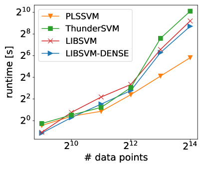
(a) CPU runtimes relative to the number of data points with $2^{10}$ features.

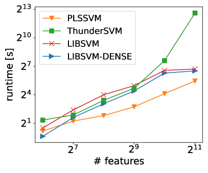
(b) CPU runtimes relative to the number of features with $2^{13}$ data points.

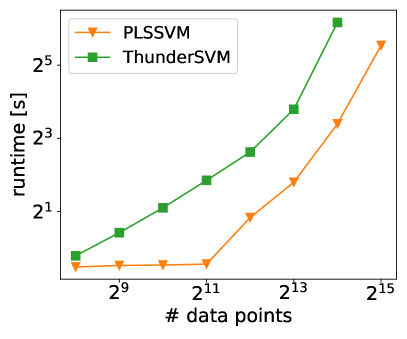
(c) GPU runtimes relative to the number of data points with $2^{12}$ features.

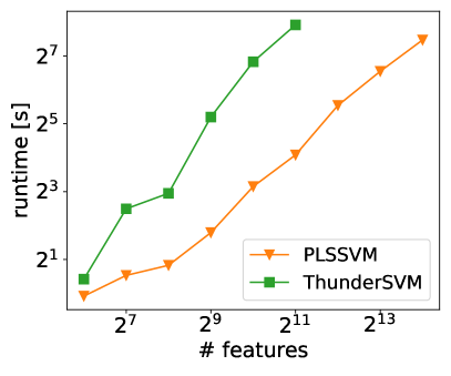
(d) GPU runtimes relative to the number of features with $2^{15}$ data points.

Figure 1: Double logarithmic runtime comparison for sparse/dense LIBSVM, ThunderSVM, and PLSSVM on both CPU and GPU in relation to the number of data points and features. The runtimes were measured with an epsilon, such that the resulting models reach approximately $97\text{\,}\frac{\mathrm{\char 37\relax}}{}$ accuracy on the training data or after convergence of the accuracy in the first three decimal places.

First, we discuss the overall runtime of our implementation using the CPU and GPU for training the SVM; see fig:runtime:compare. We only consider the linear kernel for the synthetic data sets, since the behavior can be projected one-to-one to the other kernels.

The runtime behavior for PLSSVM, ThunderSVM, and LIBSVM on the CPU, for a fixed number of features and a varying number of data points, is shown in fig:runtime:cpu:datapoints. All three SMO implementations behave very similarly, with the dense implementation of LIBSVM having a slight advantage over its sparse implementation. ThunderSVM performs better than LIBSVM in the medium size range, while in the extremes the LIBSVM variants are faster. However, all SMO implementations exhibit a steeper slope, compared to the LS-SVM method used in PLSSVM. We out-scale both LIBSVM variants, starting with $2^{11}$ data points. For $2^{14}$ data points in $2^{10}$ dimensions we need approximately $56.2\text{\,}\frac{\mathrm{s}}{}$ to train the PLSSVM while LIBSVM already needs $7.0\text{\,}\frac{\mathrm{min}}{}$ (dense) respectively $9.8\text{\,}\frac{\mathrm{min}}{}$ (sparse) and ThunderSVM performs worst with $18.3\text{\,}\frac{\mathrm{min}}{}$.

In fig:runtime:cpu:features, we examine the scalability with respect to the number of features, while the number of data points was fixed to $2^{13}$. Increasing the number of features, PLSSVM scales (up to $2^{10}$) slightly better than LIBSVM and significantly better than ThunderSVM. The behavior for the LIBSVM variants changes at $2^{12}$, but this has not been investigated further.

fig:runtime:gpu:datapoints and 1d show the same experimental setup but now using a single GPU instead of a CPU. The runtimes for PLSSVM using the GPU are orders of magnitude faster than their CPU counterpart (see fig:runtime:cpu:datapoints). PLSSVM needs about $58\text{\,}\frac{\mathrm{s}}{}$ to train a data set with $2^{14}$ data points and $2^{10}$ features on the CPU. Using a single GPU reduces this runtime by a factor of $24$ to only $2.4\text{\,}\frac{\mathrm{s}}{}$. This is surprising since both systems have a comparable computational power with $9.7\text{\,}\frac{\mathrm{TFLOPS}}{}$ theoretical peak performance for the NVIDIA A100 GPU and with $4.6\text{\,}\frac{\mathrm{TFLOPS}}{}$ (base) to $6.96\text{\,}\frac{\mathrm{TFLOPS}}{}$ (boost) for the two AMD EPYC 7742 CPUs. This underlines how much optimization potential there still is in our OpenMP implementation.

The average coefficient of variation for the SVM implementations in fig:runtime:cpu:datapoints and 1b are $0.26$ (PLSSVM), $0.92$ (ThunderSVM), $0.60$ (LIBSVM), and $0.66$ (LIBSVM-DENSE). This shows that the runtimes of our implementation have drastically less variations between executions when compared to the three SMO implementations.

fig:runtime:gpu:datapoints shows the runtimes for $2^{8}$ to $2^{15}$ data points with $2^{12}$ features each. Up to $2^{11}$ data points, the runtime of PLSSVM does not increase, indicating a significant static overhead using a GPU. However, for large data sets, this overhead is negligible (also see fig:components:datapoints). The slopes of the SVM implementations indicate that both have approximately the same overall complexity, with PLSSVM having a drastically smaller constant factor. Training the SVM model using a data set with $2^{14}$ data points needs $10\text{\,}\frac{\mathrm{s}}{}$ using PLSSVM. ThunderSVM takes $72\text{\,}\frac{\mathrm{s}}{}$, resulting in a runtime increase of a factor of $7.2$.

The differences become larger if we fix the number of data points to $2^{15}$ and vary the number of features from $2^{6}$ to $2^{14}$. This time, PLSSVM has a slightly flatter slope than ThunderSVM. ThunderSVM needs $241\text{\,}\frac{\mathrm{s}}{}$ for training a data set with $2^{11}$ features. Using PLSSVM this can be reduced by a factor of $14.2$ to only $17\text{\,}\frac{\mathrm{s}}{}$. This additionally indicates that our implementation scales better with the number of features compared to ThunderSVM. Increasing the number of features by a factor of four from $2^{11}$ to $2^{13}$ using PLSSVM, increases the runtime by a factor of roughly $5.5$. Actually, we had expected that the factor would be larger, since a four-fold increase of the number of features means an eight-fold increase of the matrix entries. However, in the selected scenario, the complexity of the problem to learn remains the same. It can thus be stated that, despite more features, fewer CG iterations are needed to solve the system of linear equations to a similar accuracy. Note that the observed performance advantage of PLSSVM over ThunderSVM thus depends to some extent on the actual classification problem.

However, it should not become as large as the factor of ThunderSVM in any case, since the complexity of the problem generally does not increase drastically with an increasing number of data points for an LS-SVM. In this example, the number of required CG iterations dropped from an average of $30.5$ iterations for a data set with $2^{10}$ points and $2^{10}$ features to only $26$ iterations for $2^{15}$ data points and the same number of features. Using ThunderSVM the runtime drastically increases by a factor of $239$ compared to the CPU runtimes.

As for the CPU runtimes, the average coefficient of variation on the GPU is again remarkably smaller for PLSSVM ($0.11$) than for ThunderSVM ($0.37$).

Looking at profiling results using NVIDIA’s Nsight Compute profiling tool, we noticed that ThunderSVM spawns a plethora of small compute kernels on the device (over $1600$ in our profiled scenario with $2^{14}$ data points and $2^{12}$ features), most of them running significantly less than one millisecond. However, the compute kernel with the highest compute intensity only reaches approximately $233\text{\,}\frac{\mathrm{GFLOPS}}{}$ which only amounts to $2.4\text{\,}\frac{\mathrm{\char 37\relax}}{}$ of the A100’s theoretical FP64 peak performance. In contrast, our implementation only spawns $3$ compute kernels that each have a much higher compute intensity than ThunderSVM’s kernels. The kernel responsible for the implicit matrix-vector multiplication inside the CG algorithm reaches over $3.1\text{\,}\frac{\mathrm{TFLOPS}}{}$ using double precision resulting in $32\text{\,}\frac{\mathrm{\char 37\relax}}{}$ FP64 peak performance.

In summary, we can note that our implementation performs comparable to the SMO implementations on the CPU and heavily outperforms ThunderSVM on the GPU.

IV-D The SAT-6 Airbone Real-World Data Set

Using the real-world data set, we observe a similar behavior. On the SAT-6 Airbone training data set, we achieved the highest accuracy with the radial basis function kernel. Training the SVM classifier using a single GPU takes $23.5\text{\,}\frac{\mathrm{min}}{}$ for our PLSSVM implementation, resulting in an accuracy of $95\text{\,}\frac{\mathrm{\char 37\relax}}{}$ on the test data set. ThunderSVM needs $40.6\text{\,}\frac{\mathrm{min}}{}$ for $94\text{\,}\frac{\mathrm{\char 37\relax}}{}$ accuracy and is thus a factor of $1.73$ slower than PLSSVM.

IV-E Runtime Analysis of the PLSSVM Components

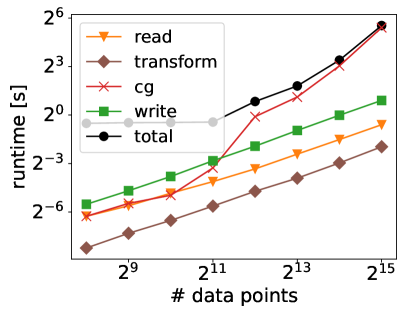
(a) GPU runtime behavior of the individual PLSSVM components depending on the number of data points with $2^{12}$ features.

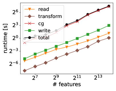
(b) GPU runtime behavior of the individual PLSSVM components depending on the number of features with $2^{15}$ data points.

Figure 2: Double logarithmic runtime scaling behavior of the individual PLSSVM components on a single GPU. The total runtime depends on the number of CG iterations, which are chosen so that the model reaches approximately $97\text{\,}\frac{\mathrm{\char 37\relax}}{}$ accuracy on the training data or after convergence of the accuracy in the first three decimal places.

fig:components breaks down the runtime of our PLSSVM library using a single GPU into its various components:

• read: Reads the input training data file and parses its content into a dense $2D$ representation.

• transform: Transforms the previously created $2D$ training data structure into a $1D$ vector in Structure-of-Arrays (SoA) layout for a better caching efficiency. This is only relevant for the GPU implementations.

• cg: In the CG component, the actual system of linear equations is solved using the selected backend.

• write: Creates and writes the resulting model file to disk.

• total: This represents the runtime of a complete training run including “read”, “transform”, “cg”, “write” and remaining parts like initializing the backend and hardware.

fig:components:datapoints shows the components’ runtimes for data set sizes from $2^{8}$ up to $2^{15}$ using $2^{12}$ features each. It can be seen that the total runtime is heavily dominated by the solution of the system of linear equations using the CG algorithm if the data set is sufficiently large enough. For data sets with less than $2^{12}$ data points, the IO components “read” and “write” contribute more to the total runtime than solving the system of linear equations. However, for a data set size of $2^{15}$, the CG algorithm is responsible for $92\text{\,}\frac{\mathrm{\char 37\relax}}{}$ of the total runtime, the other measured components combined are only accountable for $5\text{\,}\frac{\mathrm{\char 37\relax}}{}$ and, therefore, negligible. The remaining $3\text{\,}\frac{\mathrm{\char 37\relax}}{}$ of the runtime are due to parts that are not displayed here, such as the overhead when accessing the GPU for the first time or the cleanup at the end of the program execution. fig:components:datapoints shows that “read”, “transform”, and “write” do scale better than “cg” for an increasing number of data points. They can therefore also be neglected for the runtime of even larger training sets. The “cg” component has the worst complexity: doubling the number of data points increases the runtime by a factor of $3.3$.

In fig:components:features we proceed as before and fix the number of data points to $2^{15}$ while varying the number of features from $2^{6}$ to $2^{14}$. The result stays the same: solving the system of linear equations is again responsible for over $92\text{\,}\frac{\mathrm{\char 37\relax}}{}$ of the total runtime. Doubling the number of features increases the runtime by roughly a factor of $2.11$. Here, a factor of two can be justified by the fact that the effort for implicitly calculating each matrix entry doubles, since the vectors used in the scalar products have twice the size. Furthermore, the problem becomes more complex in higher dimension, so that it can be observed that more CG iterations are needed to reach a similar accuracy. Again, this factor is problem dependent. In any case, a factor larger than two is to be expected, provided that the additional features actually lift the problem into a higher dimension. First tests have indicated that the factor is close to two if the vectors are only extended with zeros.

IV-F Runtime and Accuracy Depending on Epsilon

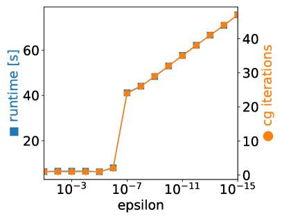
(a) Runtime and number of CG iterations relative to the relative residual.

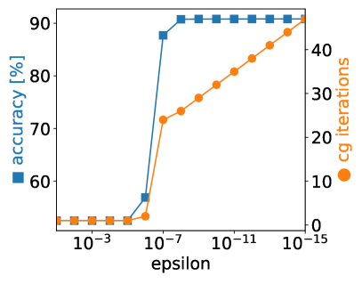
(b) Accuracy and number of CG iterations relative to the relative residual.

Figure 3: Runtime, accuracy, and number of CG iterations in relation to the relative residual of the CG method’s epsilon. Measured on the GPU machine with $2^{15}$ data points and $2^{12}$ features each.

fig:eps displays the runtime and achieved accuracy based on the chosen epsilon using a single GPU. The epsilon is used as a termination criterion in the CG algorithm. The data set contains $2^{15}$ data points with $2^{12}$ features each.

fig:eps:datapoints shows the runtime and number of CG iterations with respect to epsilon. For epsilon values up to 1e-06, the number of CG iterations does not increase significantly. Refining the epsilon $\times 0.1$ further, increases the number of CG iterations by a factor of twelve from $2$ to $24$. After that, refining the epsilon even further, steadily increases the number of CG iterations on average by $2$. As already discussed in sec:components, the total runtime is heavily dominated by solving the system of linear equations. This in turn is dominated by the number of CG iterations. Therefore, both lines lie on top of each other. This is additionally underlined by the fact that the runtime per CG iteration stays the same for data sets of the same size.

A different behavior can be observed in fig:eps:features. Here, the accuracy and number of CG iterations correlate until an epsilon of 1e-05 is reached. Afterward, the accuracy jumps to $56.9\text{\,}\frac{\mathrm{\char 37\relax}}{}$ followed by $87.6\text{\,}\frac{\mathrm{\char 37\relax}}{}$ and then reaching its final value of $90.8\text{\,}\frac{\mathrm{\char 37\relax}}{}$ for an epsilon of 1e-08. However, the number of CG iterations steadily grows from $24$ iterations for an epsilon of 1e-07 to $47$ iterations for an epsilon of 1e-15.

In general, it is nice to note that the runtime does not explode when decreasing epsilon by eight orders of magnitude from 1e-07 to 1e-15, it merely grows by a factor of about $1.83$. Thus, if a high accuracy is desired, it is fine to select a relatively small epsilon; the exact choice is not critical.

IV-G Scaling on a Many-Core CPU and Multiple GPUs

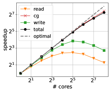
(a) Scaling behavior of the different PLSSVM components with respect to the number of cores for $2^{12}$ data points and $2^{11}$ features.

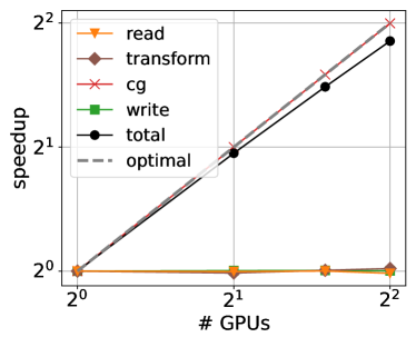
(b) Scaling behavior of the different PLSSVM components with respect to the number of GPUs for $2^{16}$ data points and $2^{14}$ features.

Figure 4: Scaling behavior with an increasing number of available hardware for the PLSSVM components on a many-core CPU and a multi-GPU system.

fig:scaling shows the scaling behavior, displayed in a double-logarithmic graph, for the different PLSSVM components with respect to the number of cores on a CPU and the number of GPUs in the system. On the CPU, only the linear kernel is plotted, since the overall scaling behaviors of the polynomial and radial kernels are the same. For the multi-GPU runs, we were only able to investigate the linear kernel, since the polynomial and radial kernels do not yet support the execution on multiple GPUs.

fig:scaling:cpu shows the speedup for the “read”, “cg”, and “write” components on a CPU with $2\cdot 64$ physical cores and $2\cdot 128$ hyper-threads using the OpenMP backend. The “transform” component is omitted since the $2D$ to $1D$ transformation is only applied for the GPU backends. The classification data set contains $2^{12}$ data points with $2^{11}$ features.

We observe that all components of our PLSSVM library scale equally well with an increasing number of available CPU cores on up to $16$ cores. The runtime decreases from $25.3\text{\,}\frac{\mathrm{min}}{}$ on a single core to $3.1\text{\,}\frac{\mathrm{min}}{}$ on $16$ cores. Using more than $64$ cores increases the runtime of the “read” and “write” components: At this point, OpenMP switches from a single socket to two sockets on our system. However, the “cg” component scales well even for up to $256$ CPU cores. In this case, the initial runtime of $25.3\text{\,}\frac{\mathrm{min}}{}$ has been reduced to $20\text{\,}\frac{\mathrm{s}}{}$, which corresponds to a parallel speedup of roughly $74.7$.

fig:scaling:gpu shows the scaling behavior of the same three components together with the “transform” component on up to four A100 GPUs using the CUDA backend. Here, the data set contains $2^{16}$ data points with $2^{14}$ features. Increasing the number of GPUs does not result in better runtimes for the “read”, “transform”, and “write” components. This is rather obvious, since none of them uses the GPUs. The “cg” component, which dominates the total runtime, is executed on the GPUs. Using four GPUs reduces the total runtime by a factor of $3.71$ from $13.49\text{\,}\frac{\mathrm{min}}{}$ to $3.72\text{\,}\frac{\mathrm{min}}{}$. This nicely demonstrates good scaling on multiple GPUs.

The total amount of memory used for the given data set on a single GPU is $8.15\text{\,}\frac{\mathrm{GiB}}{}$. Using four GPUs reduces the amount of memory used to $2.14\text{\,}\frac{\mathrm{GiB}}{}$ per GPU. While this results only in a reduction of a factor of $3.6$, instead of the optimal factor of $4$, it nevertheless shows that using multiple GPUs not only allows us to train SVM classifiers more efficient, but also to process data sets that would not fit on a single GPU. In contrast, using the same data set with ThunderSVM results in a memory consumption of $13.08\text{\,}\frac{\mathrm{GiB}}{}$ on a single GPU.

IV-H Comparison of the Implementations

To summarize, all four implementations show competitive performance for solving binary classification problems on the CPU. PLSSVM and ThunderSVM can utilize modern GPUs. ThunderSVM is restricted to GPUs from NVIDIA, as its backend is exclusively written in CUDA. PLSSVM is the only implementation supporting more than one GPU as well as GPUs from different vendors.

Since LIBSVM and ThunderSVM are well-established SVM libraries, they provide more functionality than PLSSVM so far. For example, all libraries have specific implementations for linear, polynomial, and radial basis functions kernels. In addition, LIBSVM and ThunderSVM have a sigmoid kernel and LIBSVM even supports precomputed kernels. Multi-class classification as well as regression are not yet supported by our PLSSVM library, in contrast to ThunderSVM and LIBSVM. However, it is not difficult to include these functionalities on the basis of our library if needed.

Note that the state-of-the-art SMO algorithm and the least squares approach solve slightly different optimization problems. Therefore, for a given data set, the termination criterion (epsilon) can not be reused between the two methods. This makes comparing the overall runtimes between the two approaches more difficult. In general, straightforward problems are better suited for SMO, as only few support vectors can be sufficient to compute the separating hyperplane. Difficult classification problems with plenty of data points and complex clusters that require many support vectors are better suited for the LS-SVM approach. The termination criterion for the iterative solver of our PLSSVM has to be selected suitably. However, all of our classification tasks so far have shown that the runtime is not very sensitive with respect to the termination criterion epsilon for high accuracies.

Finally, both ThunderSVM and LIBSVM support sparse data representations, which are used in their internal calculations. PLSSVM so far only supports sparse data representations when reading and writing. When parsing sparse data, we allocate memory for all features including those that are zero, resulting in a dense data representation internally.

V Conclusions and Future Work

In this work, we introduced the new SVM library PLSSVM. It is based on the rarely used least squares approach. In contrast to the SMO method that is used in most state-of-the-art implementations, it includes all data points as support vectors to compute the class-separating hyperplane. While SMO has limited parallelization potential, the LS-SVM approach is well-suited for massively parallel hardware and thus large data sets. PLSSVM is the very first SVM implementation supporting multiple backends—OpenMP, CUDA, OpenCL, and SYCL—to be able to target different hardware platforms from various vendors, being it CPUs or GPUs.

We demonstrated with classification tasks for artificial and real-world dense data sets of different sizes that we are capable of competing with well-established SMO implementations such as LIBSVM or ThunderSVM on the CPU although our basic implementation is currently still very much open to optimizations. Since there are already many widely distributed implicit matrix-vector multiplication implementations available that we have not considered yet, this shows that there is much potential for further work on a highly scalable multi-node LS-SVM implementation. On the GPU our library shows its main strength and severely outperforms ThunderSVM by a factor of $14$. We verified that our implementation scales well on many-core CPUs and multiple GPUs achieving a parallel speedup of $3.71$ on four NVIDIA A100 GPUs.

The GPU implementations have a small overhead accessing the GPU (s). Therefore, the CPU implementations are better suited for learning classifiers for very small data sets. Note that PLSSVM is currently implemented using a dense CG implementation. In the case of very sparse data sets with many features, it is therefore better to use ThunderSVM. PLSSVM clearly outperforms both LIBSVM and ThunderSVM for large non-trivial classification tasks by orders of magnitude, making use of the high parallelization potential of LS-SVMs.

Canonical next steps include the optimization of the CPU implementation, to consider sparse data structures for the CG solver, and to target multi-node multi-GPU systems to be able to use even larger data sets as currently possible and to report the scaling behavior of our library on more GPUs and CPU cores. In future work, we will investigate the advantages and disadvantages of the different backends, and provide extensive scalability studies on non-NVIDIA GPUs. As a long-term future task, we want to extend all PLSSVM kernels to support multi-node multi-GPU execution including load balancing on heterogeneous hardware. Finally, we intend to extend PLSSVM to provide all the standard functionality of LIBSVM to our users. This includes multi-class classifications and regression tasks.

References

- Chang and Lin [2011] C.-C. Chang and C.-J. Lin, “LIBSVM: A library for support vector machines,” ACM TIST, vol. 2, no. 3, pp. 1–27, 2011.
- [2] “Kaggle’s 2017 user survey,” \urlhttps://www.kaggle.com/amberthomas/kaggle-2017-survey-results/report, accessed: 2022-01-20.
- Singh et al. [2020] V. Singh et al., “Prediction of covid-19 corona virus pandemic based on time series data using support vector machine,” J. Discret. Math. Sci. Cryptogr., vol. 23, no. 8, pp. 1583–1597, 2020.
- Mahdy et al. [2020] L. N. Mahdy et al., “Automatic x-ray covid-19 lung image classification system based on multi-level thresholding and support vector machine,” MedRxiv, 2020.
- Zhu et al. [2022] B. Zhu et al., “Forecasting carbon price using a multi-objective least squares support vector machine with mixture kernels,” J. Forecast., vol. 41, pp. 100–117, 2022.
- Riyazuddin et al. [2020] Y. M. Riyazuddin et al., “Effective usage of support vector machine in face detection,” IJEAT, vol. 9, pp. 1336–1340, 2020.
- Khanday et al. [2021] A. M. U. D. Khanday et al., “Svmbpi: Support vector machine-based propaganda identification,” in Cognitive Informatics and Soft Computing. Springer Singapore, 2021, pp. 445–455.
- Boser et al. [1992] B. E. Boser et al., “A training algorithm for optimal margin classifiers,” in 5th Annual Workshop on COLT. NY, USA: ACM, 1992, pp. 144–152.
- Cortes and Vapnik [1995] C. Cortes and V. Vapnik, “Support-vector networks,” Machine Learning, vol. 20, no. 3, pp. 273–297, 1995.
- Joachims [2002] T. Joachims, Learning to Classify Text Using Support Vector Machines – Methods, Theory, and Algorithms. Kluwer/Springer, 2002.
- Platt [1998] J. Platt, “Sequential minimal optimization: A fast algorithm for training support vector machines,” Microsoft Research, techreport MSR-TR-98-14, 1998.
- Fan et al. [2008] R.-E. Fan et al., “Liblinear: A library for large linear classification,” JMLR, vol. 9, pp. 1871–1874, 2008.
- Zeng et al. [2008] Z.-Q. Zeng et al., “Fast training support vector machines using parallel sequential minimal optimization,” in 3rd Int. Conf. on ISKE, vol. 1. IEEE, 2008, pp. 997–1001.
- Wen et al. [2018] Z. Wen et al., “ThunderSVM: A fast SVM library on GPUs and CPUs,” JMLR, vol. 19, pp. 797–801, 2018.
- Carpenter [2009] A. Carpenter, “cusvm: A cuda implementation of support vector classification and regression,” \urlhttp://patternsonascreen.net/cusvm.html, pp. 1–9, 2009.
- Li et al. [2011] Q. Li et al., “Gpusvm: a comprehensive cuda based support vector machine package,” Central European Journal of Computer Science, vol. 1, no. 4, pp. 387–405, 2011.
- [17] S. Herrero, “multisvm,” \urlhttps://github.com/sergherrero/multisvm, accessed: 2022-01-20.
- Cagnin et al. [2015] H. E. L. Cagnin et al., “A portable OpenCL-based approach for SVMs in GPU,” in BRACIS. IEEE, 2015.
- Raschka et al. [2020] S. Raschka et al., “Machine learning in python: Main developments and technology trends in data science, machine learning, and artificial intelligence,” MDPI, 2020.
- [20] M. Jafferji, “svm-gpu,” \urlhttps://github.com/murtazajafferji/svm-gpu, accessed: 2022-01-20.
- Codreanu et al. [2014] V. Codreanu et al., “Evaluating automatically parallelized versions of the support vector machine,” Concurrency and Computation, vol. 28, no. 7, pp. 2274–2294, 2014.
- [22] “Sycl-ml,” \urlhttps://github.com/codeplaysoftware/SYCL-ML/, accessed: 2022-01-20.