Predicting Impact-Induced Joint Velocity Jumps on Kinematic-Controlled Manipulator
Abstract
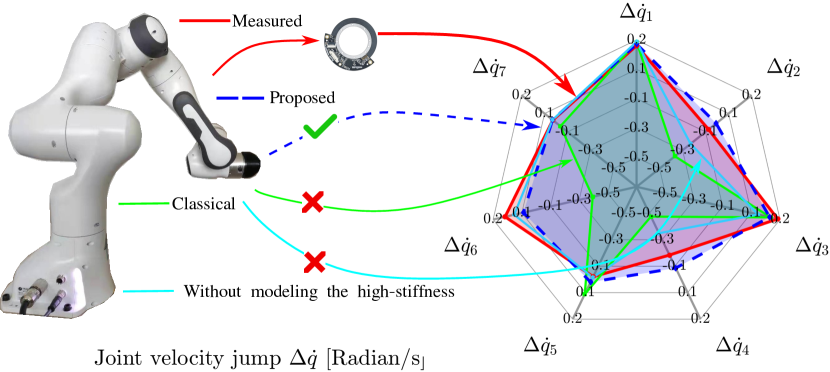
In order to enable on-purpose robotic impact tasks, predicting joint-velocity jumps is essential to enforce controller feasibility and hardware integrity. We observe a considerable prediction error of a commonly-used approach in robotics compared against 250 benchmark experiments with the Panda manipulator. We reduce the average prediction error by 81.98 as follows: First, we focus on task-space equations without inverting the ill-conditioned joint-space inertia matrix. Second, before the impact event, we compute the equivalent inertial properties of the end-effector tip considering that a high-gains (stiff) kinematic-controlled manipulator behaves like a composite-rigid body.
Index Terms:
Contact modeling, Dynamics, Industrial Robots.I Introduction
We aim at enabling robots to impact with the highest feasible velocity111Refer to Impact-Aware Manipulation https://i-am-project.eu. An impact-aware robot controller must embed predicted post-impact joint velocities to prevent violation of hardware limitations [1]. To our best knowledge, existing prediction approaches are not well-assessed with a rich ground-truth, e.g., based on large impact-data collected from high-gain joint-velocity (or -position) controlled robots, we refer to as kinematic controlled robots.
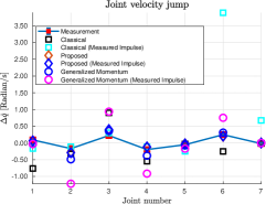
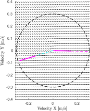
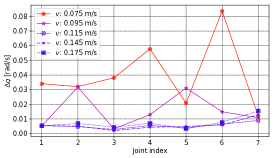
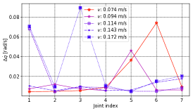
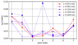
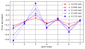
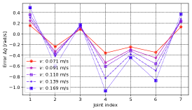
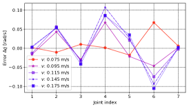
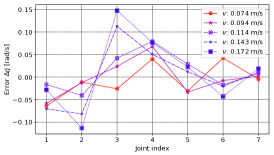
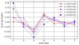
The methodology proposed in the late 1980s [2] predicts the impact-induced joint-velocity jumps as the product of the inverted joint-space inertia matrix (JSIM) and the joint-space impulse, see also [3, 4]. Unfortunately, this prediction scheme poorly matches the measurements collected from our benchmark experiments, see Fig. 1.
We summarize three reasons that potentially explain such discrepancies:
R1) Inaccurate impulse calculation:
accurate task-space impulse calculation222We reserve prediction for the concept: predicting the joint velocity jumps. Thus, we use impulse calculation to describe impulse prediction. is essential for solving the joint velocity jumps from momentum conservation; i.e., the momentum change is equal to the impulse. The classical approach relies on inaccurate calculation [5, Fig. 9], which overestimates the normal impulse and does not account for contact friction effects [6, Eq. 4.8], [7].
R2) Ill-conditioned JSIM:
The computation is sensitive to the impulse-calculation error since it inverts the ill-conditioned JSIM.
Featherstone [8] summarized that the condition number of the JSIM grows within the range of and for a serial robotic manipulator with being the number of revolute joints. Therefore, the inverted JSIM amplifies errors associated with the impulse [8, Chapter 10.1].
R3) Unmodeled joint-stiffness behavior:
Standard robot manipulators are mechanically stiff (not backdrivable) and kinematic-controlled to precisely track reference trajectories [4, Chapter 9].
The joint velocity jump prediction in [2, 3, 4] does not account for either mechanical non-backdrivability or high-gain PD control (quasi-locked joints) in drivable ones. Both induces rather light-flexibilities of the joints as acknowledged in [9, 10], and recently in [5, Fig. 9].
Since three-dimensional impact dynamics models are not well-assessed for articulated robots [6, 7], we use the measured impulses, or compute the normal impulse with our improved calculation [5] when the tangential impulse is negligible (R1). We formulate the momentum conservation in the task-space. Hence, our approach does not involve the joint-space formulation relying on the JSIM (R2). We modify the task-space impulse-to-velocity mapping considering the joints to be stiff at impact and therefore behaving as a composite-rigid body (CRB) (R3), yet at a time flexible to allow potential post-impact contact mode as sliding/sticking.
We conducted 250 impact experiments with the seven degrees of freedom Panda manipulator for evaluation. The dataset comprises different impact configurations, various normal and tangential contact velocities. We repeat each condition ten times to eliminate the outliers. The proposed prediction:
-
•
outperforms the classical approach, reducing the average prediction error by ;
-
•
is analytical, i.e., does not require the measured impulse. The average prediction error remains on the same level whether the impulse is calculated or measured.
Interested readers can reproduce our results with the post-processed data and the MATLAB scripts333https://gite.lirmm.fr/yuquan/fidynamics/-/wikis/Predicting-Impact-Induced-Sudden-Change-of-Joint-Velocities.
II Related work
Impacts affect the robot joint velocities almost instantly [2]. Preemptive actions are necessary to avoid violating the hardware-dependent joint velocity bounds. Unlike specifying pre- and post-impact velocity references in joint space [12] or planning impacts carefully [13], it is generally more convenient to formulate quadratic optimization problems in task-space to meet multiple control objectives and constraints [14]. We preliminarily enabled on-purpose impacts to second order dynamic QP control schemes [1, 15].
Most of the impact dynamics models focus on the velocity jumps in Cartesian space [6, 16, 17], e.g., batting a flying object [16]. Solving the joint velocity jumps merely serves as an intermediate step concerning the momentum conservation in joint-space [2, 11, 18]. Our literature review revealed that the algebraic equations for the joint-space velocity jumps proposed by [2] more than 30 years ago are still considered state-of-the-art, see e.g., the robotics textbook [4] and the survey by [3]. They are used recently in [19], to extract the rigid impact component in the post-impact joint-velocity oscillatory-behavior (a corotational impact approach).
However, to the authors’ best knowledge, the prediction of joint-space velocity jumps has not been confronted to ground-truth experiments with manipulators that are kinematic-controlled. Also, our former QP controller extension was assessed in simulation only [1].
Hereafter, we list some issues of the usual computation:
Impulse calculation
Integrating an impact dynamics model into QP controllers is not trivial. Formulating optimization problems requires closed-form constraints and objectives that are not possible with friction. There exist analytical solutions only for the planar impacts [18]. When the variables are constrained on a plane, the analytical solution exists because the post-impact contact mode is limited to rebounce, sliding, reverse sliding, and sticking [6, 18, 16]. Without a numerical process, it is not possible to determine the tangential velocities for three-dimensional impacts [6, 7].
Ill-conditioning issue
The principle of momentum conservation is often specified in joint space, relying on the joint-space inertia matrix (JSIM). The JSIM inversion [2] amplifies the impulse calculation errors [8, Chapter 10.1] due to the well-known ill-conditioning issue of the JSIM [20]. Real-robot experiments we conducted proved that incorporating the JSIM inversion for dynamically consistent null-space projections does not significantly show, in practice, theoretical-conceptual superiority [21, 22]. That is why a recent line of research proposed alternative orthogonal null-space projectors that do not rely on the inverted JSIM [23].
Unmodeled joint-stiffness behavior
Early works since the 1990s focus on contact-force modeling for one degree-of-freedom set-up [9], or control designs to damp the post-impact oscillations [10, 24] using compliant models. Textbook impact mechanics usually assume impacts between two free-flying objects [6, 7]. Unfortunately, most existing joint-velocity-jump predictions do not explicitly account for the joint stiffness at impact, or even consider under-actuated pendulums [11, 25]. We preliminarily concluded that the CRB assumption is essential for task-space velocity-to-impulse calculation for a kinematic-controlled robot [5]. Otherwise, merely fulfilling the joint motion constraint [11, 18] underestimates the equivalent momentum at the manipulator contact point [5, Fig. 9]. We therefore adopt the CRB assumption from [5] for the task-space impulse-to-velocity mapping.
III Background
The well-known equations of motion (EOM) for a fixed-base manipulator with degrees of freedom are given as , where gathers the centrifugal, Coriolis, and gravitational forces, denotes the joint actuation torques and denotes the external force applied on a contact point. We denote the positive-definite JSIM as , and the translation (linear) part of the contact point Jacobian as .
Problem statement: How to accurately predict the impact-induced joint velocity jumps , given prior knowledge of the (pre-)impact robot configuration, i.e., (i) the joint positions , velocities , (ii) the equations of motion, (iii) the contact point location with its associated and (iv) an impact dynamics model that predicts the task-space impulse
| (1) |
where we compute the task-space velocity jump based on the coefficient of restitution and the pre-impact velocity :
We assume that:
-
1.
The impact force is dominant relatively to other forces. Consequently, generalized forces such as the centrifugal forces or motor command torques during impact are negligible [6, Chapter 8.1.1].
-
2.
The contact area is tiny compared to the robot dimensions such that a point contact model is appropriate [26].
- 3.
-
4.
The robot manipulator is fully actuated under kinematic control with high gains.
-
5.
The manipulator has a minimum of three degrees of freedom. It impacts at the end-effector, and the joint configuration at impact is not in a singular configuration.
In the rest of the paper, we represent the contact velocity and the impulse in the contact frame . The origin of locates at the contact point. The -axis aligns with the impact normal. The -axis and -axis span the tangential plane.
Remark III.1
We handle velocity and wrench transforms in line with the geometric approach stated in [27]. The notation Ad is the abbreviation of adjoint transform [27, Lemma 2.13 on page 56], which is associated with rigid body motion . We use to transform twists from one coordinate to another. For instance, we transform the wrench measured from the contact point frame to the centroidal frame :
III-A The usual approach
Integrating the EOM over the impact duration leads to the impulse-momentum conservation in joint space:
| (2) |
where is . We have , due to assumption 1. The usual approach [2, 3, 4] predicts by left multiplying (2) with :
| (3) |
which is the product of and the joint-space impulse . The impulse in (3) is unknown. Left multiplying (3) by yields:
| (4) |
where the product is positive-definite and invertible due to assumption 5. The classical approach predicts the task-space impulse as [2, 3, 4]:
| (5) |
Substituting the calculated impulse (5) into (3), the predicted joint velocity jump is:
| (6) |
which is equivalently written in a weighted least-squares form:
| (7) |
| (a) Configuration one | (b) The measured |
| (c) Configuration two | (d) The measured |
| (e) Configuration three | (f) The measured |
III-B The inaccurate impulse issue
We showed in our earlier work [5, Fig. 9] that the impulse calculation (5) is inaccurate as it overestimates the normal impulse . Even more problematic, the calculation (5) does not fulfill Coulomb’s friction cone since it does not take the friction coefficient into account.
Example 1
When the impact is frictionless , the tangential impulse is zero [7, Sec. 2.4]. Given the joint positions corresponding to the impact configurations in Fig. 2(a), 2(c), 2(e) and the coefficient of restitution and , equation (5) predicts:
| (8) |
where the reference contact velocity expressed in the end-effector coordinates is: m/s. It is obvious that the tangential impulses in (8) do not match .
III-C The ill-conditioning issue
Implementing the JSIM inversion in practice leads to critical numerical issues. The inversion amplifies errors of in proportion to the high condition number of the JSIM; see the sources of numerical errors reported by Featherstone [8, Chapter 10.1], [20, Sec. 2]. The high condition number of is an underlying property of the mechanism itself. Inline with the analysis in [20], we obtain the following values on the order of with for the impact configurations shown in Fig. 2(a), 2(c), 2(e):
| (9) |
Similar, large condition numbers are reported for the KUKA LBR iiwa manipulator with seven joints [22, Fig. 8].
III-D Unmodeled stiffness issue
We clarified in our earlier work that the impulse calculation is not accurate without considering stiffness behavior [5]. However, the classical approach (7) merely imposes the joint motion constraint
| (10) |
without modifying the task-space impulse-to-velocity mapping:
| (11) |
which is embeded in the intermediate step (4). Given the same task-space impulse, (11) predicts the same contact velocity jump for (1) a high-gain joint-position-controlled robot, and (2) a compliant pure joint-torque-controlled robot.
IV Novel Prediction of Joint Velocity Jumps
In response to the above issues, we (i) adopt the improved impulse calculation relying on the CRB assumption [5], see Sec. IV-A; (ii) avoid the JSIM inversion by solving from momentum conservation equations in the task-space, see Sec. IV-B; and (iii) modify the task-space impulse-to-velocity mapping assuming the robot is a composite-rigid body prior to the impact, see Sec. IV-C.
IV-A Impulse calculation
IV-B Momentum conservation in the task-space
Given the equivalent inertia matrix , the Newton-Euler’s equations at the contact point are [27, Eq. 4.16][8, Eq. 2.68]:
| (13) |
where is the rotational velocity, is the rotational moment, and we adopt the six-dimensional cross product [8]. Integrating (13) over the impact duration , and neglecting the centrifugal and Coriolis forces concerning assumption 1, yields
| (14) |
where (assumption 3). Define as the corner matrix of , we left-multiply to (14):
| (15) |
Substituting the joint motion constraint (10) into (15) yields
| (16) |
Now, we obtain in a least-squares form
| (17) |
which does not rely on the critical JSIM inversion.
IV-C Imposing the composite-rigid-body assumption
We compute the equivalent inertia matrix at the contact point based on the CRB assumption. Defining the centroidal frame between the inertial frame and the contact frame , the body velocity444 is noted by in [27]. We omit the subscript b since we only use body velocities. associated with the rigid motion writes [27, Proposition 2.15]:
| (18) |
where is the relative velocity [28]. According to the CRB assumption, we impose zero relative velocity . Thus, we approximate:
| (19) |
where transforms from to .
Given the centroidal inertia [28] , the centroidal momentum is:
where transforms from to . Substituting into (19), we have
The linear part of is the contact velocity in its body coordinates555Note that representing a quantity in a far-away coordinate frame introduces another source of numerical error [8, Chapter 10.1]. . Thus, we extract the linear part (the upper-left matrix) of
to have the IIM :
| (20) |
where is the CRB moment of inertia, and are the rotation and translation respectively, between the COM and the contact point. The skew-symmetric matrix represents the cross product as matrix multiplication.
V Data Acquisition
We collected a large amount of impact data with the FrankaEmika Panda robot in order to thoroughly evaluate and compare the three predictions . Specifying the contact velocities in the inertial frame , we conducted two types of impact experiments:
- 1.
-
2.
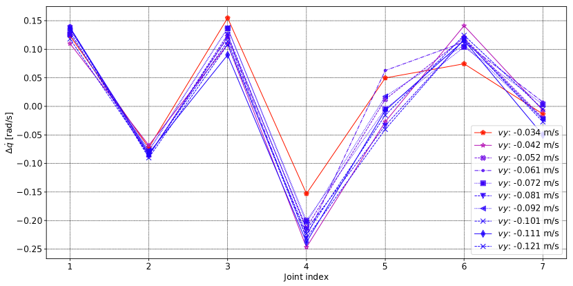
Commanding the normal contact velocity m/s, the robot applied an increasing tangential velocity , , , , , , , , , m/s with the end-effector while keeping m/s. When the impact took place, the joint postures in all the situations were close to Fig. 2(a).
Repeating each configuration ten times, we collected 150 experiments in the first case and another 100 experiments in the second case666We presented the contact-force profiles of the 150 experiments in our earlier work [5] for normal impulse calculation. In this paper, we present the joint velocity jumps collected from the same 150 experiments. The data of the other 100 experiments have been specifically collected for this article..
We compute utilizing the mean measurement , of the ten repetitions in each configuration777We apply the Panda robot model documented at https://github.com/jrl-umi3218/mc_panda., and compared to the corresponding mean measurement . The , and were consistent within the repetitions. The standard deviation of , are rad and rad/s, respectively. The standard deviation of measured is higher, yet still small, see Fig. 9.
We measured the ground-truth impulse with an ATI-mini45 force-torque sensor. It can capture the impact dynamics with a sampling rate of 25000 Hz without low-pass filtering. We apply the average measured impulse from ten identical experiments to remove the random effects.
The friction coefficient for all experiments is . The impulse fulfills Coulomb’s friction cone [6, 7, Eq. 4.8]:
| (24) |
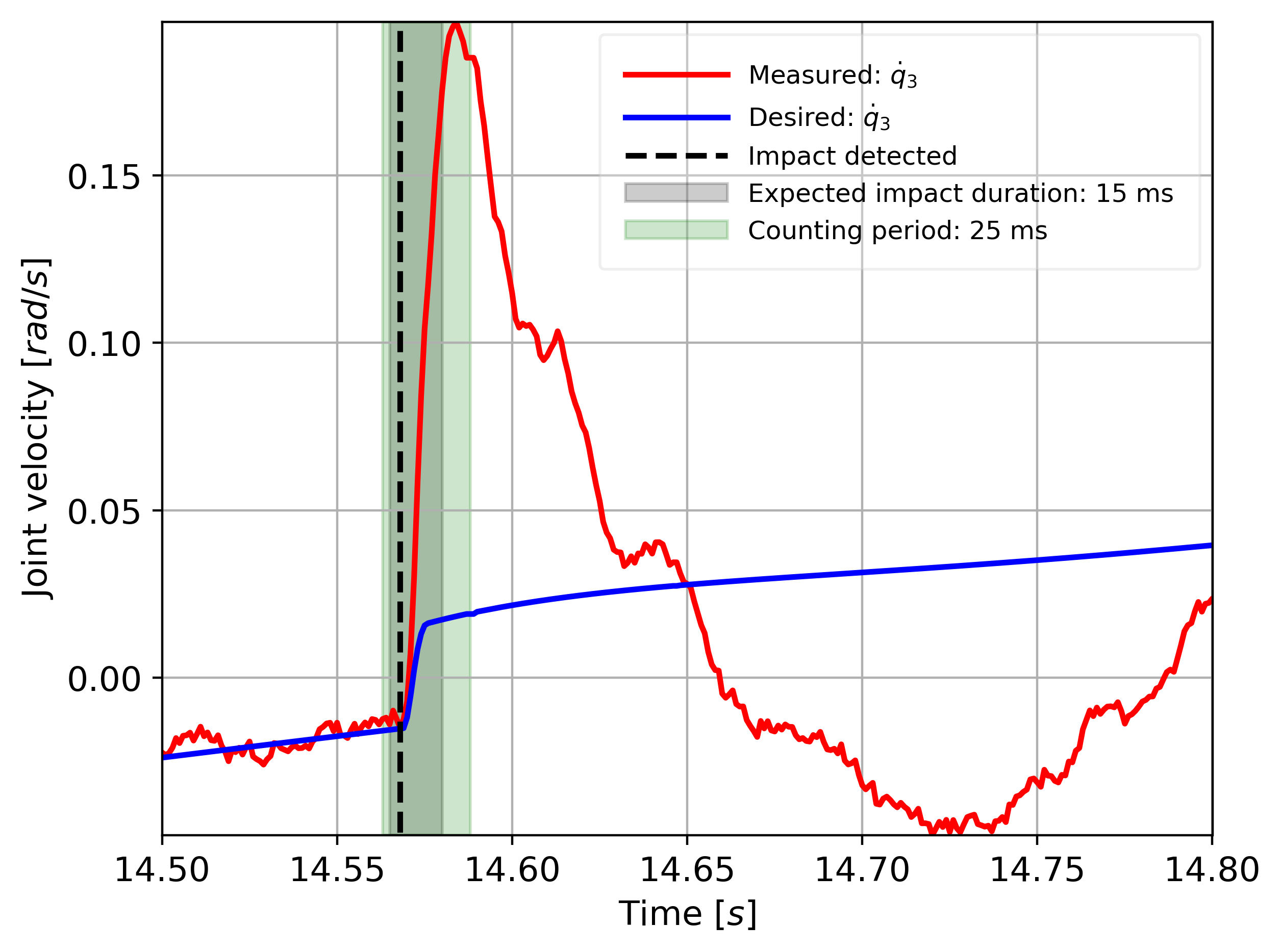
Regardless of the joint configurations or contact velocities, the impact duration was about 15 ms on average, and 25 ms at maximum for the Panda robot [5, Fig. 6]. The control cycle was 1 ms. Upon contact detection, the controller immediately pulled back the end-effector along the contact normal.
V-A Measuring the joint velocity jumps
The impact-detection time is to ms by thresholding the joint torque error [5, Sec. VI]. In order to measure the joint velocity jumps , we search for in a conservative time window, covering 5 ms before and 20 ms after the impact detection; see Fig. 3.
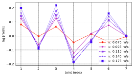
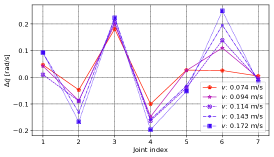
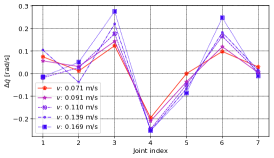
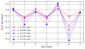
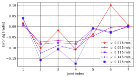
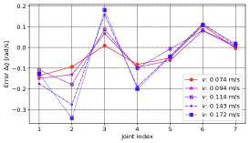
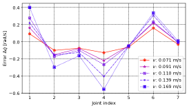
We plot the mean of the measured in Fig. 8. Given the increasing reference normal contact velocities m/s, the magnitude of for increases without changing the sign (jump direction).
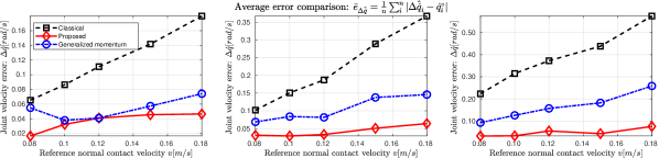
V-B Prediction error definitions
VI Comparison results and discussion
The first set of experiments reveal that:
- •
-
•
only requires analytical computation. It is robust to impulse-calculation errors, Sec. VI-A.
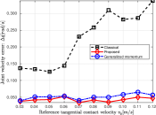
The second set of experiments reveal that:
-
•
The proposed prediction applies to non-zero tangential velocities, see Sec. VI-B1.
We apply the impulse calculation (12) for and with and , respectively. We ignore the tangential component of for due to the discussion in Sec. III-B. The contact mode was sliding in all the experiments due to the discussion in Sec. VI-B2.
| Reference: | m/s | m/s | m/s | m/s | m/s |
| The proposed solution average error (21) | |||||
| Fig. 2(a) | |||||
| Fig. 2(c) | |||||
| Fig. 2(e) | |||||
| The classical solution average error (6) | |||||
| Fig. 2(a) | |||||
| Fig. 2(c) | |||||
| Fig. 2(e) | |||||
| The generalized-momentum average solution (23) | |||||
| Fig. 2(a) | |||||
| Fig. 2(c) | |||||
| Fig. 2(e) | |||||
VI-A Robustness to impulse-calculation errors
We denote the measured impulse as . According to our former benchmark experiments [5, Fig. 9], is most-close-to . Further, is less than the measured impulse while overestimates. Concerning the impulse calculation errors, we substituted the measured impulse (instead of the predicted impulse) into the different approaches for comparison. We denote the predictions after the substitution as: (6), (23), and (21).
The substitution introduced a considerable impulse correction for the classical prediction and the solution without considering high-stiffness behaviours .
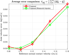
Given the errors on the left side of Fig. 5, the accuracy of or decreases. Compared to , the performance decrease of is even worse due to the high condition number of the JSIM.
keeps a similar average error concerning the right side of Fig. 5. Since the only difference between computing and is the choice of or , we conclude outperforms because of the CRB assumption.
VI-B Contact mode and pre-impact tangential velocities
VI-B1 Non-zero pre-impact tangential velocities
Despite (12) cannot predict the tangential impulse, the prediction is robust to pre-impact tangential velocities in our experiments when the friction coefficient .
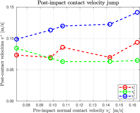
VI-B2 Sliding contact
We compute the post-impact tangential velocities using the measured joint velocity jump and the kinematics (10). Given are non-zero in Fig. 7, the contact mode was sliding at and after the impact. The robot is able to slide because the manipulator is mounted on a fixed-base, during the impact event the joint motion is compliant to the rigid wall despite the robot is high-gain controlled.
For impacts between two free-flying objects, sliding happens if the friction coefficient is smaller than the stick coefficient [6, Eq. 4.12] [7, Sec. 5], i.e., the friction is not enough to sustain the contact. Using the joint configuration in Fig. 2(c) as an example, we have:
| (27) |
where is computed by substituting into [6, Eq. 4.12].
VII Conclusion
Predicting joint velocity jumps is paramount to achieve the highest feasible contact velocity while fulfilling the hardware resilience bounds. Our approach (i) uses our improved normal impulse calculation [5]; (ii) avoids inverting the ill-conditioned JSIM by formulating momentum conservation equations in task space; and (iii) modifies the task-space impulse-to-velocity mapping to account for a high-gain (stiff) joint behavior in pre- and at impact, while allowing flexibility in post-impact. As a result, from benchmarking 250 impact experiments our proposed prediction (21) reduces the average prediction error by 81.98 w.r.t the existing approach.
Future work is dedicated to tangential impulse calculation and impact propagation in robotic structures.
Acknowledgment
This work is supported by the EU H2020 research grant GA 871899, I.AM. project. We would like to thank Mohamed Djeha and Saeid Samadi for the valuable feedback.
References
- [1] Y. Wang and A. Kheddar, “Impact-friendly robust control design with task-space quadratic optimization,” in Robotics: Science and Systems, vol. 15, no. 32, Freiburg, Germany, 24-26 June 2019.
- [2] Y.-F. Zheng and H. Hemami, “Mathematical modeling of a robot collision with its environment,” Journal of Field Robotics, vol. 2, no. 3, pp. 289–307, 1985.
- [3] J. W. Grizzle, C. Chevallereau, R. W. Sinnet, and A. D. Ames, “Models, feedback control, and open problems of 3d bipedal robotic walking,” Automatica, vol. 50, no. 8, pp. 1955–1988, 2014.
- [4] B. Siciliano and O. Khatib, Springer handbook of robotics. Springer, 2016.
- [5] Y. Wang, N. Dehio, and A. Kheddar, “On inverse inertia matrix and contact-force model for robotic manipulators at normal impacts,” IEEE Robotics and Automation Letters, vol. 7, no. 2, pp. 3648–3655, 2022.
- [6] W. J. Stronge, Impact mechanics. Cambridge university press, 2000.
- [7] Y.-B. Jia and F. Wang, “Analysis and computation of two body impact in three dimensions,” Journal of Computational and Nonlinear Dynamics, vol. 12, no. 4, 2017.
- [8] R. Featherstone, Rigid body dynamics algorithms. Springer, 2008.
- [9] K. Youcef-Toumi and D. Gutz, “Impact and force control: Modeling and experiments,” Journal of dynamic systems, measurement, and control, vol. 116, no. 1, pp. 89–98, 1994.
- [10] G. Ferretti, G. Magnani, and A. Z. Rio, “Impact modeling and control for industrial manipulators,” IEEE Control Systems Magazine, vol. 18, no. 4, pp. 65–71, 1998.
- [11] H. M. Lankarani, “A poisson-based formulation for frictional impact analysis of multibody mechanical systems with open or closed kinematic chains,” Journal of Mechanical Design, vol. 122, no. 4, pp. 489–497, 2000.
- [12] M. Rijnen, E. de Mooij, S. Traversaro, F. Nori, N. van de Wouw, A. Saccon, and H. Nijmeijer, “Control of humanoid robot motions with impacts: Numerical experiments with reference spreading control,” in IEEE Int. Conf. on Robotics and Automation, 2017, pp. 4102–4107.
- [13] T. Stouraitis, L. Yan, J. Moura, M. Gienger, and S. Vijayakumar, “Multi-mode trajectory optimization for impact-aware manipulation,” in IEEE/RSJ Int. Conf. on Intelligent Robots and Systems, 2020, pp. 9425–9432.
- [14] K. Bouyarmane, K. Chappellet, J. Vaillant, and A. Kheddar, “Quadratic programming for multirobot and task-space force control,” IEEE Transactions on Robotics, 2019.
- [15] Y. Wang, D. Niels, A. Tanguy, and A. Kheddar, “Impact-aware task-space quadratic-programming control,” 2020. [Online]. Available: https://arxiv.org/pdf/2006.01987.pdf
- [16] Y.-B. Jia, M. Gardner, and X. Mu, “Batting an in-flight object to the target,” The Int. Journal of Robotics Research, vol. 38, no. 4, pp. 451–485, 2019.
- [17] S. Faik and H. Witteman, “Modeling of impact dynamics: A literature survey,” in 2000 Int. ADAMS User Conf., vol. 80. Citeseer, 2000.
- [18] Y. Khulief, “Modeling of impact in multibody systems: an overview,” Journal of Computational and Nonlinear Dynamics, vol. 8, no. 2, 2013.
- [19] I. Aouaj, V. Padois, and A. Saccon, “Predicting the post-impact velocity of a robotic arm via rigid multibody models: an experimental study,” in IEEE Int. Conf. on Robotics and Automation, 2021, pp. 2264–2271.
- [20] R. Featherstone, “An empirical study of the joint space inertia matrix,” The Int. Journal of Robotics Research, vol. 23, no. 9, pp. 859–871, 2004.
- [21] A. Dietrich, C. Ott, and A. Albu-Schäffer, “An overview of null space projections for redundant, torque-controlled robots,” Int. Journal of Robotics Research, vol. 34, no. 11, pp. 1385–1400, 2015.
- [22] M. d. P. A. Fonseca, B. V. Adorno, and P. Fraisse, “Task-space admittance controller with adaptive inertia matrix conditioning,” Journal of Intelligent & Robotic Systems, vol. 101, no. 2, pp. 1–19, 2021.
- [23] N. Dehio, J. Smith, D. L. Wigand, P. Mohammadi, M. Mistry, and J. J. Steil, “Enabling impedance-based physical human–multi–robot collaboration: Experiments with four torque-controlled manipulators,” The Int. Journal of Robotics Research, 2021.
- [24] W. Xu, J. Han, and S. Tso, “Experimental study of contact transition control incorporating joint acceleration feedback,” IEEE/ASME transactions on mechatronics, vol. 5, no. 3, pp. 292–301, 2000.
- [25] S. Ganguly and O. Khatib, “Contact-space resolution model for a physically consistent view of simultaneous collisions in articulated-body systems: theory and experimental results,” The Int. Journal of Robotics Research, vol. 39, no. 10-11, pp. 1239–1258, 2020.
- [26] A. Chatterjee and A. Ruina, “A new algebraic rigid-body collision law based on impulse space considerations,” Journal of Applied Mechanics, vol. 65, no. 4, pp. 939–951, 1998.
- [27] R. M. Murray, Z. Li, S. S. Sastry, and S. S. Sastry, A mathematical introduction to robotic manipulation. CRC press, 1994.
- [28] D. E. Orin, A. Goswami, and S.-H. Lee, “Centroidal dynamics of a humanoid robot,” Autonomous robots, vol. 35, no. 2-3, pp. 161–176, 2013.