The Hamiltonian Extended Krylov Subspace Method

Abstract

An algorithm for constructing a $J$-orthogonal basis of the extended Krylov subspace $\mathcal{K}_{r,s}=\operatorname{range}\{u,Hu,H^{2}u,$ $\ldots,$ $H^{2r-1}u,H^{-1}u,H^{-2}u,\ldots,H^{-2s}u\},$ where $H\in\mathbb{R}^{2n\times 2n}$ is a large (and sparse) Hamiltonian matrix is derived (for $r=s+1$ or $r=s$). Surprisingly, this allows for short recurrences involving at most five previously generated basis vectors. Projecting $H$ onto the subspace $\mathcal{K}_{r,s}$ yields a small Hamiltonian matrix. The resulting HEKS algorithm may be used in order to approximate $f(H)u$ where $f$ is a function which maps the Hamiltonian matrix $H$ to, e.g., a (skew-)Hamiltonian or symplectic matrix. Numerical experiments illustrate that approximating $f(H)u$ with the HEKS algorithm is competitive for some functions compared to the use of other (structure-preserving) Krylov subspace methods.

65F25, 65F50, 65F60, 15A23.

1 Introduction

Let $H\in\mathbb{R}^{2n\times 2n}$ be a nonsingular (large-scale) Hamiltonian matrix, that is $J_{n}H=(J_{n}H)^{T},$ where $J_{n}=\left[\begin{smallmatrix}0&I_{n}\\ -I_{n}&0\end{smallmatrix}\right]\in\mathbb{R}^{2n\times 2n}$ and $I_{n}$ is the $n\times n$ identity matrix. We are interested in computing a $J$-orthogonal basis of the extended Krylov subspace

(1.1) $$\mathcal{K}_{r,s} :=\mathcal{K}_{2r}(H,u)+\mathcal{K}_{2s}(H^{-1},H^{-1}u)=\operatorname{range}\{u,Hu,H^{2}u,\ldots,H^{2r-1}u,H^{-1}u,H^{-2}u,\ldots,H^{-2s}u\},$$

where $u\in\mathbb{R}^{2n}$ and either $r=s+1$ or $r=s.$ That is, assuming

$$\operatorname{dim}\mathcal{K}_{2r}(H,u)=2r\quad\text{ and }\quad\operatorname{dim}\mathcal{K}_{2s}(H^{-1},H^{-1}u)=2s,$$

we are looking for a matrix $S_{r+s}\in\mathbb{R}^{2n\times 2(r+s)}$ with $J$-orthonormal columns ($S_{r+s}^{T}J_{n}S_{r+s}=J_{r+s}$) such that the columns of $S_{r+s}$ span the same subspace as $\mathcal{K}_{2r}(H,u)+\mathcal{K}_{2s}(H^{-1},H^{-1}u).$

Extended Krylov subspaces

$$\operatorname{range}\{b,A^{-1}b,Ab,A^{-2}b,A^{2}b,\ldots,A^{-k}b,A^{k}b\}=\mathcal{K}_{k}(A,b)+\mathcal{K}_{k}(A^{-1},A^{-1}b)$$

for general nonsingular matrices $A\in\mathbb{C}^{n\times n}$ and a vector $b\in\mathbb{C}^{n}$ have been used for the numerical approximation of $f(A)b$ for a function $f$ and a large matrix $A$ at least since the late 1990s mainly inspired by [7, 15]. In case an orthogonal matrix $V$ has been constructed such that $\operatorname{range}(V)=\mathcal{K}_{k}(A,b)+\mathcal{K}_{k}(A^{-1},A^{-1}b),$ an approximation to $f(A)b$ can be obtained as

(1.2) $$f(A)b\approx Vf(V^{T}AV)V^{T}b.$$

More on functions of matrices, the computation of $f(A)b$ and the approximation of $f(a)b$ via Krylov subspace methods can be found in the all-encompassing monograph [14].

The idea of constructing a $J$-orthogonal basis for the extended Krylov subspace $\mathcal{K}_{r,s}$ (1.1) has first been considered in [20] in the context of approximating $\exp(H)u.$ The Hamiltonian Extended Krylov Subspace (short HEKS) method presented in [20] is a straightforward adaption of the algorithm for computing an orthogonal basis of an extended Krylov subspace described in [15]. Our main finding in this paper is the observation that the HEKS algorithm allows for a short recurrence to generate $S_{r+s}.$

We will explore the use of an $J$-orthogonal basis $S_{r+s}$ of the extended Krylov subspace $\mathcal{K}_{r,s}$ (1.1) for approximating $f(H)u$ for a (large-scale) Hamiltonian matrix $H$ and a vector $u\in\mathbb{R}^{2n}.$ Following the idea from (1.2) we have

$$f(H)u\approx S_{r+s}f(H_{r+s})J_{r+s}^{T}S_{r+s}^{T}J_{n}u$$

where $H_{r+s}=J_{r+s}^{T}S_{r+s}^{T}J_{n}HS_{r+s}\in\mathbb{R}^{2(r+s)\times 2(r+s)}$ is a Hamiltonian matrix. That is, we can preserve the rich structural information inherent to the Hamiltonian structure of the matrix $H$. This would not be possible by computing a standard (orthogonal) basis $V\in\mathbb{R}^{2n\times 2(r+s)}$ of $\mathcal{K}_{r,s}$ as the matrix product $V^{T}HV$ will in general not be a Hamiltonian matrix even if $H$ is Hamiltonian. Hence, the HEKS algorithm may be used in particular in order to approximate $f(H)u$ where $f$ is a function which maps the Hamiltonian matrix $H$ to a structured matrix such as a (skew-)Hamiltonian or symplectic matrix. Such a structure-preserving approximation of $f(H)u$ is, e.g., important in the context of symplectic exponential integrators for Hamiltonian systems, see, e.g., [8, 10, 19, 20]. A structure-preserving approximation of $f(H)u$ may also be computed using, e.g., an $J$-orthogonal basis $\tilde{S}_{2k}$ of the standard Krylov subspace $\operatorname{range}\{u,Hu,H^{2}u\ldots,H^{2k-1}u\}.$ Such a basis can be generated by the Hamiltonian Lanczos method [4, 5, 22]. Both approaches will be compared later on.

The paper is structured as follows: Section 2 summarizes some basic well-known facts about Hamiltonian and $J$-orthogonal matrices. In Section 3 the general idea of generating the desired $J$-orthogonal basis $S_{r+s}$ of (1.1) as proposed in [20] is sketched. Then, it is noted that the projected matrices $H_{r+s}=J_{r+s}^{T}S_{r+s}^{T}J_{n}HS_{r+s}$ and $J_{r+s}^{T}S_{r+s}^{T}J_{n}H^{-1}S_{r+s}$ have at most $10k,$ resp. $10k+2$, nonzero entries. The details are given in Section 4 and in Section 5. The resulting efficient HEKS algorithm using short recursions is summarized in Section 6. The rather long and technical constructive proof for our claim is deferred to the Appendix A. In Section 7 the approximation of $f(H)u$ using the HEKS algorithm is compared to the approximation by the extended Krylov subspace method [16] and by the Hamiltonian Lanczos method [5].

2 Preliminaries

Here we list some properties of Hamiltonian and $J$-orthogonal matrices useful for the following discussion.

1. $J_{n}=\left[\begin{smallmatrix}0&I_{n}\\ -I_{n}&0\end{smallmatrix}\right]\in\mathbb{R}^{2n\times 2n}$ is orthogonal and skew-symmetric, $J_{n}^{T}=J_{n}^{-1}=-J_{n}$.

2. Let $H\in\mathbb{R}^{2n\times 2n}.$ $H$ is Hamiltonian if and only if there exist matrices $E$, $B=B^{T}$, $C=C^{T}$ $\in\mathbb{R}^{n\times n}$ such that

   $$H=\begin{bmatrix}E&B\\ C&-E^{T}\end{bmatrix}.$$

3. Let $H\in\mathbb{R}^{2n\times 2n}$ be a nonsingular Hamiltonian matrix. Then $H^{-1}$ is Hamiltonian as well.

4. The eigenvalues of a Hamiltonian matrix $H$ occur in pairs $\{\lambda,-\lambda\}$ if $\lambda$ is real or purely imaginary, or in quadruples $\{\lambda,\overline{\lambda},-\lambda,-\overline{\lambda}\}$ otherwise. That is, the spectrum of a Hamiltonian matrix is symmetric with respect to both the real and the imaginary axis.

5. A matrix $S\in\mathbb{R}^{2n\times 2n}$ is called symplectic if $S^{T}J_{n}S=J_{n}$. Its columns are $J$-orthogonal.

6. Let $S\in\mathbb{R}^{2n\times 2n}$ be a symplectic matrix. Then $S^{-1}=J_{n}^{T}S^{T}J_{n}$ is symplectic as well.

7. Let $H\in\mathbb{R}^{2n\times 2n}$ be a Hamiltonian matrix and $S\in\mathbb{R}^{2n\times 2n}$ be a symplectic matrix. Then $S^{-1}HS$ is a Hamiltonian matrix.

8. Let $S\in\mathbb{R}^{2n\times 2m},m\leq n,$ have $J$-orthogonal columns, $S^{T}J_{n}S=J_{m}.$ Let $H\in\mathbb{R}^{2n\times 2n}$ be Hamiltonian.

   1. The matrix $J_{m}^{T}S^{T}J_{n}$ is the left inverse of $S$, $J_{m}^{T}S^{T}J_{n}S=I_{2m}.$

   2. The matrix $(J_{m}^{T}S^{T}J_{n})HS$ is Hamiltonian.

Numerous further properties of the sets of these matrices (and their interplay) have been studied in the literature, see, e.g., [17] and the references therein. In particular, $J_{n}$ induces a skew-symmetric bilinear form $\langle\cdot,\cdot\rangle_{J_{n}}$ on $\mathbb{R}^{2n}$ defined by $\langle x,y\rangle_{J_{n}}=y^{T}J_{n}x$ for $x,y\in\mathbb{R}^{2n}.$ Hamiltonian matrices are skew-adjoint with respect to the bilinear form $\langle\cdot,\cdot\rangle_{J_{n}}$, while symplectic matrices are orthogonal with respect to $\langle\cdot,\cdot\rangle_{J_{n}}$. The $2n\times 2n$ symplectic matrices form a Lie group, the $2n\times 2n$ Hamiltonian matrices the associated Lie algebra.

Assume that a matrix $S_{k}=[V_{k}\leavevmode\nobreak\ \leavevmode\nobreak\ W_{k}]\in\mathbb{R}^{2n\times 2k}$ with $J$-orthogonal columns is given with $V_{k}=[v_{1}\leavevmode\nobreak\ \leavevmode\nobreak\ v_{2}\leavevmode\nobreak\ \leavevmode\nobreak\ \cdots\leavevmode\nobreak\ \leavevmode\nobreak\ v_{k}]$ and $W_{k}=[w_{1}\leavevmode\nobreak\ \leavevmode\nobreak\ w_{2}\leavevmode\nobreak\ \leavevmode\nobreak\ \cdots\leavevmode\nobreak\ \leavevmode\nobreak\ w_{k}]\in\mathbb{R}^{2n\times k}$. Two additional vectors $x,J_{n}x\in\mathbb{R}^{2n}$ can be added to $S_{k}$ to generate a matrix $S_{k+1}=[V_{k+1}\leavevmode\nobreak\ \leavevmode\nobreak\ W_{k+1}]\in\mathbb{R}^{2n\times 2k+2}$ with $J$-orthogonal columns by $J$-orthogonalizing the vectors $x$ and $J_{n}x$ against all column vectors $v_{j},w_{j}$ of $S_{k}$ via

$$v_{k+1} =x-S_{k}J_{k}^{T}S_{k}^{T}J_{n}x,$$

$$w_{k+1} =(J_{n}v_{k+1})-S_{k}J_{k}^{T}S_{k}^{T}J_{n}(J_{n}v_{k+1}),\quad w_{k+1}=w_{k+1}/(v_{k+1}^{T}J_{n}w_{k+1}).$$

3 Idea of the HEKS Algorithm

Let a Hamiltonian matrix $H\in\mathbb{R}^{2n\times 2n}$ and a vector $u_{1}\in\mathbb{R}^{2n},$ $\|u_{1}\|_{2}=2,$ be given. Assume that $\operatorname{dim}\mathcal{K}_{2r}(H,u_{1})=2r$ and $\operatorname{dim}\mathcal{K}_{2s}(H^{-1},H^{-1}u_{1})=2s$. The goal is to construct a matrix $S_{r+s}\in\mathbb{R}^{2n\times 2(r+s)}$ with $J$-orthonormal columns ($S_{r+s}^{T}J_{n}S_{r+s}=J_{r+s}$) such that the columns of $S_{r+s}$ span the same subspace as $\mathcal{K}_{2r}(H,u_{1})+\mathcal{K}_{2s}(H^{-1},H^{-1}u_{1}).$

In [20] it is suggested to construct the matrix $S_{r+s}$ in the following way (assuming that no breakdown occurs):

1. We start with the two vectors in $\mathcal{K}_{2}(H,u_{1})$ and construct

   $$S_{1}=\begin{bmatrix}u_{1}\mid v_{1}\end{bmatrix}\in\mathbb{R}^{2n\times 2}$$

   with $S_{1}^{T}J_{n}S_{1}=J_{1}$ and $\operatorname{range}\{S_{1}\}=\mathcal{K}_{2}(H,u_{1}).$ This corresponds to the choice $r=1,s=0.$

2. Thereafter we take the two vectors in $\mathcal{K}_{2}(H^{-1},H^{-1}u_{1})$ and construct

   $$S_{2}=\begin{bmatrix}y_{1}&u_{1}\mid x_{1}&v_{1}\end{bmatrix}=\begin{bmatrix}Y_{1}&U_{1}\mid X_{1}&V_{1}\end{bmatrix}\in\mathbb{R}^{2n\times 4}$$

   with $S_{2}^{T}J_{n}S_{2}=J_{2}$ and $\operatorname{range}\{S_{2}\}=\mathcal{K}_{2}(H,u_{1})+\mathcal{K}_{2}(H^{-1},H^{-1}u_{1}).$ This corresponds to the choice $r=s=1.$

We proceed in this fashion by alternating between the subspaces $\mathcal{K}_{2r}(H,u_{1})$ and $\mathcal{K}_{2s}(H^{-1},H^{-1}u_{1}).$ Assume that a matrix

$$S_{2k}=\begin{bmatrix}Y_{k}&U_{k}\mid X_{k}&V_{k}\end{bmatrix}\in\mathbb{R}^{2n\times 4k},\qquad Y_{k},U_{k},X_{k},V_{k}\in\mathbb{R}^{2n\times k}$$

with $J$-orthonormal columns has been constructed such that its columns span the same space as $\mathcal{K}_{2k}(H,u_{1})+\mathcal{K}_{2k}(H^{-1},H^{-1}u_{1}).$ The following three steps are repeated until the desired symplectic basis has been generated:

• Construct $u_{k+1}$ and $v_{k+1}$ and set

  $$S_{2k+1} =\begin{bmatrix}Y_{k}&U_{k}&u_{k+1}\mid X_{k}&V_{k}&v_{k+1}\end{bmatrix}=\begin{bmatrix}Y_{k}&U_{k+1}\mid X_{k}&V_{k+1}\end{bmatrix}\in\mathbb{R}^{2n\times 4k+2}$$

  with

  $$U_{k+1}=\begin{bmatrix}U_{k}&u_{k+1}\end{bmatrix},V_{k+1}=\begin{bmatrix}V_{k}&v_{k+1}\end{bmatrix}\in\mathbb{R}^{2n\times k+1}$$

  such that $S_{2k+1}^{T}J_{n}S_{2k+1}=J_{2k+1}$ and $\operatorname{range}\{S_{2k+1}\}=\mathcal{K}_{2k+2}(H,u_{1})+\mathcal{K}_{2k}(H^{-1},H^{-1}u_{1}).$ The new vectors are added as the last column to the $U,$ resp. $V$-matrix.

• Construct $y_{k+1}$ and $x_{k+1}$ and set

  $$S_{2k+2} =\begin{bmatrix}y_{k+1}&Y_{k}&U_{k+1}\mid x_{k+1}&X_{k}&V_{k+1}\end{bmatrix}=\begin{bmatrix}Y_{k+1}&U_{k+1}\mid X_{k+1}&V_{k+1}\end{bmatrix}\in\mathbb{R}^{2n\times 4k+4}$$

  with

  $$Y_{k+1}=\begin{bmatrix}y_{k+1}&Y_{k}\end{bmatrix},X_{k+1}=\begin{bmatrix}x_{k+1}&X_{k}\end{bmatrix}\in\mathbb{R}^{2n\times k+1}$$

  such that $S_{2k+2}^{T}J_{n}S_{2k+2}=J_{2k+2}$ and $\operatorname{range}\{S_{2k+2}\}=\mathcal{K}_{2k+2}(H,u_{1})+\mathcal{K}_{2k+2}(H^{-1},H^{-1}u_{1}).$ The new vectors are added as the first column to the $Y$, resp. $X$-matrix.

• Set $k=k+1.$

We refrain from restating the algorithm given in [20] which implements the approach stated above in a straightforward way using long recurrences. As usual, a Krylov recurrence of the form

$$HS_{2k}=S_{2k}H_{2k}+\text{ some rest term},$$

for $r=s=k$ and

$$HS_{2k+1}=S_{2k+1}H_{2k+1}+\text{some rest term}$$

for $r=s+1=k$ holds, where $H_{2k}=J_{2k}^{T}S_{2k}^{T}J_{n}HS_{2k}\in\mathbb{R}^{4k\times 4k}$ and $H_{2k+1}=J_{2k+1}^{T}S_{2k+1}^{T}J_{n}HS_{2k+1}\in\mathbb{R}^{4k+2\times 4k+2}$ are Hamiltonian matrices. In the next two sections we describe the very special forms of the projected matrices $H_{2k}$ and $H_{2k+1}$ as well as $J_{2k}^{T}S_{2k}^{T}J_{n}H^{-1}S_{2k}$ and $J_{2k+1}^{T}S_{2k+1}^{T}J_{n}H^{-1}S_{2k+1}.$ These matrices have at most $10k,$ resp. $10k+2$, nonzero entries. A constructive proof for our claim is given in Appendix A, while the resulting efficient HEKS algorithm using short recursions is summarized in Section 6.

4 Projection $J_{r+s}^{T}S_{r+s}^{T}J_{n}HS_{r+s}$ of the Hamiltonian matrix $H$

Assume that

$$S_{r+s}=\begin{bmatrix}Y_{s}&U_{r}\mid X_{s}&V_{r}\end{bmatrix},\qquad Y_{s},X_{s}\in\mathbb{R}^{2n\times s},\quad U_{r},V_{r}\in\mathbb{R}^{2n\times r},$$

with $J$-orthogonal columns has been constructed with the HEKS algorithm (as before, we assume that $r=s$ or $r=s+1$). Then the projected Hamiltonian matrix

$$H_{r+s}=J_{r+s}^{T}S_{r+s}^{T}J_{n}HS_{r+s}\in\mathbb{R}^{2(r+s)\times 2(r+s)}$$

has a very special form with at most $2r+8s$ nonzero entries. Let us first note that

$$H_{r+s}={\small\begin{bmatrix}-X_{s}^{T}J_{n}HY_{s}&-X_{s}^{T}J_{n}HU_{r}&-X_{s}^{T}J_{n}HX_{s}&-X_{s}^{T}J_{n}HV_{r}\\ -V_{r}^{T}J_{n}HY_{s}&-V_{r}^{T}J_{n}HU_{r}&-V_{r}^{T}J_{n}HX_{s}&-V_{r}^{T}J_{n}HV_{r}\\ Y_{s}^{T}J_{n}HY_{s}&Y_{s}^{T}J_{n}HU_{r}&Y_{s}^{T}J_{n}HX_{s}&Y_{s}^{T}J_{n}HV_{r}\\ U_{r}^{T}J_{n}HY_{s}&U_{r}^{T}J_{n}HU_{r}&U_{r}^{T}J_{n}HX_{s}&U_{r}^{T}J_{n}HV_{r}\end{bmatrix}},$$

where the blocks are of size either $s\times s,$ $r\times r,$ $s\times r,$ or $r\times s.$ As will be proven in Appendix A, ten of these blocks are zero, three are diagonal (denoted by $\Delta_{s},\Theta_{r},\Lambda_{s}$), one symmetric tridiagonal (denoted by $T_{r}$) and two anti-bidiagonal (denoted by $B_{sr}$), i.e.,

(4.3) $$H_{r+s}=\begin{bmatrix}0&0&\Lambda_{s}&B_{sr}\\ 0&0&B_{sr}^{T}&T_{r}\\ \Delta_{s}&0&0&0\\ 0&\Theta_{r}&0&0\end{bmatrix}$$

with

$$\Delta_{s} =\operatorname{diag}(\delta_{s},\ldots,\delta_{1})\in\mathbb{R}^{s\times s},$$

$$\Theta_{r} =\operatorname{diag}(\vartheta_{1},\ldots,\vartheta_{r})\in\mathbb{R}^{r\times r},$$

$$\Lambda_{s} =\operatorname{diag}(\lambda_{s},\ldots,\lambda_{1})\in\mathbb{R}^{s\times s},$$

$$T_{r} =\begin{bmatrix}\alpha_{1}&\beta_{2}&&\\ \beta_{2}&\ddots&\ddots&\\ &\ddots&\ddots&\beta_{r}\\ &&\beta_{r}&\alpha_{r}\end{bmatrix}\in\mathbb{R}^{r\times r},$$

and either

$$B_{r-1,r}=\begin{bmatrix}&&&\gamma_{r-1}&\mu_{r}\\ &&\iddots&\mu_{r-1}&\\ &\iddots&\iddots&&\\ \gamma_{1}&\mu_{2}&&&\end{bmatrix}\in\mathbb{R}^{r-1\times r}\quad\text{\leavevmode\nobreak\ \leavevmode\nobreak\ if \leavevmode\nobreak\ \leavevmode\nobreak\ }r=s+1,$$

or

$$B_{rr}=\begin{bmatrix}&&&\gamma_{r}\\ &&\iddots&\mu_{r}\\ &\iddots&\iddots&\\ \gamma_{1}&\mu_{2}&\end{bmatrix}\in\mathbb{R}^{r\times r}\quad\text{\leavevmode\nobreak\ \leavevmode\nobreak\ if \leavevmode\nobreak\ \leavevmode\nobreak\ }r=s.$$

In particular, it holds for $j=1,\ldots,s$

$$\delta_{j} =y_{j}^{T}J_{n}Hy_{j},\qquad\lambda_{j}=-x_{j}^{T}J_{n}Hx_{j},$$

and for $j=1,\ldots,r$

$$\vartheta_{j} =u_{j}^{T}J_{n}Hu_{j},\qquad\alpha_{j}=-v_{j}^{T}J_{n}Hv_{j},\qquad\gamma_{j}=-x_{j}^{T}J_{n}Hv_{j},$$

and for $j=2,\ldots,r$

$$\beta_{j} =-v_{j}^{T}J_{n}Hv_{j-1}\qquad \mu_{j} =-x_{j-1}^{T}J_{n}Hv_{j}.$$

We summarize this in the following theorem.

Theorem 4.1.

Let $H\in\mathbb{R}^{2n\times 2n}$ be a Hamiltonian matrix. Let $r+s=n$ and either $r=s+1$ or $r=s.$ Then in case the procedure described in Section 3 does not break down for $u_{1}\in\mathbb{R}^{2n}$ with $\|u_{1}\|_{2}=1$ there exists a symplectic matrix $S\in\mathbb{R}^{2n\times 2n}$ such that $Se_{s+1}=u_{1},$

$$\operatorname{range}\{S\}=\mathcal{K}_{2r}(H,u_{1})+\mathcal{K}_{2s}(H^{-1},H^{-1}u_{1}),$$

and

$$S^{-1}HS=H_{r+s}$$

with $H_{r+s}=H_{n}$ as in (4.3).

Proof.

A constructive proof is given in Section A.

Remark 4.2.

In case the Hamiltonian matrix $H$ can be written in the form $H=JK$ with the symmetric matrix $K$ and $K$ is positive definit, all inner products of the form $w^{T}JHw$ and $w^{T}JH^{-1}w$ are negative, as $w^{T}JHw=w^{T}JJKw=-w^{T}Kw<0$ and as with $K$ its inverse is symmetric and positive definite. Thus, in this case, all $\delta_{j}$ and $\vartheta_{j}$ are negative, while all $\lambda_{j}$ and $\alpha_{j}$ are positive. Such Hamiltonian matrices have been considered in [1, 2].

Theorem 4.1 implies

$$H\begin{bmatrix}Y_{k}&U_{k}&X_{k}&V_{k}\end{bmatrix} =S\left[\begin{array}[]{c|c||c|c}0&0&0&0\\ 0&0&\Lambda_{k}&B_{kk}\\ \hline\cr 0&0&B_{kk}^{T}&T_{k}\\ 0&0&\mu_{k+1}e_{1}^{T}&\beta_{k+1}e_{k}^{T}\\ 0&0&0&0\\ \hline\cr\hline\cr 0&0&0&0\\ \Delta_{k}&0&0&0\\ \hline\cr 0&\Theta_{k}&0&0\\ 0&0&0&0\\ \end{array}\right].$$

From this, we obtain the HEKS-recursion for $r=s=k$

(4.4) $$HS_{2k} =S_{2k}H_{2k}+\mu_{k+1}u_{k+1}e_{2k+1}^{T}+\beta_{k+1}u_{k+1}e_{4k}^{T},$$

while for $r=s+1=k+1$ we have

(4.5) $$HS_{2k+1} =S_{2k+1}H_{2k+1}+(\gamma_{k+1}y_{k+1}+\beta_{k+2}u_{k+2})e_{4k+2}^{T}.$$

5 Projection $J_{r+s}^{T}S_{r+s}^{T}J_{n}H^{-1}S_{r+s}$ of the Hamiltonian matrix $H^{-1}$

Assume that Theorem 4.1 holds. As $H_{n}=S^{-1}HS\in\mathbb{R}^{2n\times 2n}$ is Hamiltonian, its inverse $H_{n}^{-1}=S^{-1}H^{-1}S$ is Hamiltonian as well. Not only $H_{n}$ has a nice sparse structure (4.3), but also its inverse. From that we can derive the special forms of $J_{2k}^{T}S_{2k}^{T}J_{n}H^{-1}S_{2k}$ and $J_{2k+1}^{T}S_{2k+1}^{T}J_{n}H^{-1}S_{2k+1}.$

Let $S=S_{n}=\begin{bmatrix}Y_{s}&U_{r}\mid X_{s}&V_{r}\end{bmatrix}\in\mathbb{R}^{2n\times 2n},$ $Y_{s},X_{s}\in\mathbb{R}^{2n\times s},$ $U_{r},V_{r}\in\mathbb{R}^{2n\times r},$ where $r+s=n$ and either $r=s$ or $r=s+1.$ Due to $S_{n}^{-1}=J_{n}^{T}S_{n}^{T}J_{n},$ we have

$$H_{n}^{-1} ={\small\begin{bmatrix}-X_{s}^{T}J_{n}H^{-1}Y_{s}&-X_{s}^{T}J_{n}H^{-1}U_{r}&-X_{s}^{T}J_{n}H^{-1}X_{s}&-X_{s}^{T}J_{n}H^{-1}V_{r}\\ -V_{r}^{T}J_{n}H^{-1}Y_{s}&-V_{r}^{T}J_{n}H^{-1}U_{r}&-V_{r}^{T}J_{n}H^{-1}X_{s}&-V_{r}^{T}J_{n}H^{-1}V_{r}\\ Y_{s}^{T}J_{n}H^{-1}Y_{s}&Y_{s}^{T}J_{n}H^{-1}U_{r}&Y_{s}^{T}J_{n}H^{-1}X_{s}&Y_{s}^{T}J_{n}H^{-1}V_{r}\\ U_{r}^{T}J_{n}H^{-1}Y_{s}&U_{r}^{T}J_{n}H^{-1}U_{r}&U_{r}^{T}J_{n}H^{-1}X_{s}&U_{r}^{T}J_{n}H^{-1}V_{r}\end{bmatrix}}$$

$$=\begin{bmatrix}0&0&\Delta_{s}^{-1}&0\\ 0&0&0&\Theta_{r}^{-1}\\ E_{s}&G_{sr}&0&0\\ G_{sr}^{T}&F_{r}&0&0\end{bmatrix}$$

with $E_{s}\in\mathbb{R}^{s\times s},$ $F_{r}\in\mathbb{R}^{r\times r},$ $G_{sr}\in\mathbb{R}^{s\times r}$ such that

$$\begin{bmatrix}\Lambda_{s}&B_{sr}\\ B_{sr}^{T}&T_{r}\end{bmatrix}\begin{bmatrix}E_{s}&G_{sr}\\ G_{sr}^{T}&F_{r}\end{bmatrix}=I$$

holds and $\Delta_{s},\Theta_{r},\Lambda_{s},T_{r},B_{sr}$ from (4.3). The matrices $E_{s},F_{r}$ and $G_{sr}$ have a special structure like $\Lambda_{s},T_{r}$ and $B_{sr}$: $F_{r}$ is diagonal, $G_{sr}$ anti-bidiagonal as $B_{sr}$ and $E_{s}$ is symmetric tridiagonal;

$$F_{r} =\operatorname{diag}(f_{11},f_{22},\ldots,f_{rr}),\qquad E_{s}=\begin{bmatrix}e_{ss}&e_{s-1,s}&&&\\ e_{s-1,s}&\ddots&\ddots&&\\ &\ddots&\ddots&e_{12}&\\ &&e_{12}&e_{11}\end{bmatrix}=E_{s}^{T},$$

and either

$$G_{r-1,r}=\begin{bmatrix}&&&g_{r-1,r-1}&g_{r-1,r}\\ &&\iddots&g_{r-2,r-1}&\\ &g_{22}&\iddots&&\\ g_{11}&g_{12}&&&\end{bmatrix}\in\mathbb{R}^{r-1\times r}\quad\text{\leavevmode\nobreak\ \leavevmode\nobreak\ if \leavevmode\nobreak\ \leavevmode\nobreak\ }r=s+1,$$

or

$$G_{rr}=\begin{bmatrix}&&&g_{rr}\\ &&\iddots&g_{r-1,r}\\ &g_{22}&\iddots&\\ g_{11}&g_{12}&\end{bmatrix}\in\mathbb{R}^{r\times r}\quad\text{\leavevmode\nobreak\ \leavevmode\nobreak\ if \leavevmode\nobreak\ \leavevmode\nobreak\ }r=s.$$

Next, the projected matrices $J_{2k}^{T}S_{2k}^{T}J_{n}H^{-1}S_{2k}$ and $J_{2k+1}^{T}S_{2k+1}^{T}J_{n}H^{-1}S_{2k+1}$ will be described. Let

$$\mathfrak{E}_{j}=\begin{bmatrix}I_{j}\\ 0\end{bmatrix}\in\mathbb{R}^{r\times j},\qquad\mathfrak{F}_{\ell}=\begin{bmatrix}0\\ I_{\ell}\end{bmatrix}\in\mathbb{R}^{s\times\ell},\qquad\mathfrak{T}_{\ell j}=\begin{bmatrix}\mathfrak{F}_{\ell}\\ &\mathfrak{E}_{j}\\ &&\mathfrak{F}_{\ell}\\ &&&\mathfrak{E}_{j}\end{bmatrix}\in\mathbb{R}^{2n\times 2(\ell+j)}$$

for $j\leq r,$ $\ell\leq s.$ Thus, for $2k\leq n$ it holds

$$S_{n}\mathfrak{T}_{kk}=S_{2k}\in\mathbb{R}^{2n\times 4k}\qquad\text{and}\qquad S_{n}\mathfrak{T}_{k,k+1}=S_{2k+1}\in\mathbb{R}^{2n\times 4k+2},$$

as well as

$$S_{n}J_{n}\mathfrak{T}_{kk} =\begin{bmatrix}-X_{k}&-V_{k}&Y_{k}&U_{k}\end{bmatrix}=S_{2k}J_{2k}\in\mathbb{R}^{2n\times 4k},$$

$$S_{n}J_{n}\mathfrak{T}_{k,k+1} =\begin{bmatrix}-X_{k}&-V_{k+1}&Y_{k}&U_{k+1}\end{bmatrix}=S_{2k+1}J_{2k+1}\in\mathbb{R}^{2n\times 4k+2}.$$

Hence, we obtain

$$J_{2k}^{T}S_{2k}^{T}J_{n}H^{-1}S_{2k} =\mathfrak{T}_{kk}^{T}J_{n}^{T}S_{n}^{T}J_{n}H^{-1}S_{n}\mathfrak{T}_{kk}=\mathfrak{T}_{kk}^{T}H_{n}^{-1}\mathfrak{T}_{kk}=\mathfrak{T}_{kk}^{T}\begin{bmatrix}0&0&\Delta_{s}^{-1}&0\\ 0&0&0&\Theta_{r}^{-1}\\ E_{s}&G_{sr}&0&0\\ G_{sr}^{T}&F_{r}&0&0\end{bmatrix}\mathfrak{T}_{kk}$$

(5.6) $$=\begin{bmatrix}0&0&\mathfrak{F}_{k}^{T}\Delta_{s}^{-1}\mathfrak{F}_{k}&0\\ 0&0&0&\mathfrak{E}_{k}^{T}\Theta_{r}^{-1}\mathfrak{E}_{k}\\ \mathfrak{F}_{k}^{T}E_{s}\mathfrak{F}_{k}&\mathfrak{F}_{k}^{T}G_{sr}\mathfrak{E}_{k}&0&0\\ \mathfrak{E}_{k}^{T}G_{sr}^{T}\mathfrak{F}_{k}&\mathfrak{E}_{k}^{T}F_{r}\mathfrak{E}_{k}&0&0\end{bmatrix}=\begin{bmatrix}0&0&\Delta_{k}^{-1}&0\\ 0&0&0&\Theta_{k}^{-1}\\ E_{k}&G_{kk}&0&0\\ G_{kk}^{T}&F_{k}&0&0\end{bmatrix}$$

and

(5.7) $$J_{2k+1}^{T}S_{2k+1}^{T}J_{n}H^{-1}S_{2k+1} =\mathfrak{T}_{k,k+1}^{T}J_{n}^{T}S_{n}^{T}J_{n}H^{-1}S_{n}\mathfrak{T}_{k,k+1}=\begin{bmatrix}0&0&\Delta_{k}^{-1}&0\\ 0&0&0&\Theta_{k+1}^{-1}\\ E_{k}&G_{k,k+1}&0&0\\ G_{k,k+1}^{T}&F_{k+1}&0&0\end{bmatrix}.$$

The HEKS-recurrences for $H^{-1}$ are given by

(5.8) $$H^{-1}S_{2k}=S_{2k}\left(J_{2k}^{T}S_{2k}^{T}J_{n}H^{-1}S_{2k}\right)+(e_{2k,2k+1}x_{2k+1}+g_{2k,2k+1}v_{2k+1})e_{1}^{T}$$

and

(5.9) $$H^{-1}S_{2k+1}=S_{2k+1}\left(J_{2k+1}^{T}S_{2k+1}^{T}J_{n}H^{-1}S_{2k+1}\right)+x_{2k+1}(e_{2k,2k+1}e_{1}^{T}+g_{2k+1,2k+1}e_{2k+1}^{T}).$$

6 HEKS Algorithm

The HEKS algorithm is summarized in Fig. 1. The algorithm as given assumes that no breakdown occurs. Clearly, any division by zero will result in a serious breakdown. As can be seen from (4.4) a lucky breakdown occurs in case $\mu_{k+1}=\beta_{k+1}=0$ or $u_{k+1}=0$, as $\operatorname{range}\{S_{2k}\}=\mathcal{K}_{2k}(H,u_{1})+\mathcal{K}_{2k}(H^{-1},H^{-1}u_{1})$ is $H$-invariant. Moreover, (4.5) shows that in case $\gamma_{k+1}=\beta_{k+2}=0,$ a lucky breakdown occurs, as $\operatorname{range}\{S_{2k+1}\}=\mathcal{K}_{2k+2}(H,u_{1})+\mathcal{K}_{2k}(H^{-1},H^{-1}u_{1})$ is $H$-invariant. Similarly, lucky breakdown can be read off of (5.8) and (5.9) resulting in an $H^{-1}$-invariant subspace.

In case the Hamiltonian matrix $H$ can be written in the form $H=JK$ with a symmetric positive definite matrix $K$, all inner products of the form $w^{T}JHw$ and $w^{T}JH^{-1}w$ are negative (see Remark 4.2). Hence, most scalars by which is divided in Algorithm 1 are nonzero and do not cause breakdown.

Implemented efficiently such that each matrix-vector product as well as each linear solve is computed only once, the algorithm requires (for adding $4$ vectors) in the for-loop

• $4$ matrix-vector-multiplications with $H$,

• $3$ linear solves with $H$ (efficiently implemented in the form $(JH)x=(Jb)$ making use of the symmetry of $JH$),

• $14$ scalar products.

Any multiplication of a vector $w$ by $J_{n}$ should be implemented by rearranging the upper and the lower part of the vector $w$. That is, let $w=\left[\begin{smallmatrix}w_{1}\\ w_{2}\end{smallmatrix}\right],$ then $J_{n}w=\left[\begin{smallmatrix}w_{2}\\ -w_{1}\end{smallmatrix}\right].$

Without some form of re-$J$-orthogonalization the HEKS algorithm suffers from the same numerical difficulties as any other Krylov subspace method.

Algorithm 1 HEKS with short recurrences

1:Hamiltonian matrix $H{\in}\mathbb{R}^{2n\times 2n}$, $u_{1}{\in}\mathbb{R}^{2n}$ with $\|u_{1}\|_{2}=1$

2:a) $S_{2k}=[y_{k}\leavevmode\nobreak\ \cdots\leavevmode\nobreak\ y_{1}\leavevmode\nobreak\ u_{1}\leavevmode\nobreak\ \cdots\leavevmode\nobreak\ u_{k}\mid x_{k}\leavevmode\nobreak\ \cdots\leavevmode\nobreak\ x_{1}\leavevmode\nobreak\ v_{1}\leavevmode\nobreak\ \cdots\leavevmode\nobreak\ v_{k}\in\mathbb{R}^{2n\times 4k}$ with $S_{2k}^{T}J_{n}S_{2k}=J_{2k}$ and $H_{2k}=J_{2k}S_{2k}^{T}J_{n}HS_{2k}$ as in (4.3)
b) parameters $\lambda_{j},\delta_{j},\alpha_{j},\gamma_{j},\vartheta_{j}$ for $j=1,\ldots,k$ and $\beta_{j},\mu_{j}$ for $j=2,\ldots,k$ which determine $H_{2k}$
(for $S_{2k+1}\in\mathbb{R}^{2n\times 4k+2}$ the algorithm needs to be modified appropriately)

3:$u_{1}=u_{1}/\|u_{1}\|_{2}$ $\triangleright$ Set up $S_{1}=[u_{1}\mid v_{1}]$

4:$\vartheta_{1}=u_{1}^{T}J_{n}Hu_{1}$

5:$v_{1}=Hu_{1}/\vartheta_{1}$

6:$f_{11}=u_{1}^{T}J_{n}H^{-1}u_{1}$$\triangleright$ Set up $S_{2}=[y_{1}\leavevmode\nobreak\ u_{1}\mid x_{1}\leavevmode\nobreak\ v_{1}]$

7:$w_{x}=H^{-1}u_{1}-f_{11}v_{1}$

8:$x_{1}=w_{x}/\|w_{x}\|_{2}$

9:$y_{1}=H^{-1}x_{1}/x_{1}^{T}J_{n}H^{-1}x_{1}$

10:$\lambda_{1}=-x_{1}^{T}J_{n}Hx_{1}$ and $\delta_{1}=y_{1}^{T}J_{n}Hy_{1}$

11:$\alpha_{1}=-v_{1}^{T}J_{n}Hv_{1}$ and $\gamma_{1}=-x_{1}^{T}J_{n}Hv_{1}$$\triangleright$ Set up $S_{3}=[y_{1}\leavevmode\nobreak\ u_{1}\leavevmode\nobreak\ u_{2}\mid x_{1}\leavevmode\nobreak\ v_{1}\leavevmode\nobreak\ v_{2}]$

12:$w_{u}=Hv_{1}-\gamma_{1}y_{1}-\alpha_{1}u_{1}$

13:$u_{2}=w_{u}/\|w_{u}\|_{2}$

14:$\vartheta_{2}=u_{2}^{T}J_{n}Hu_{2}$

15:$v_{2}=Hu_{2}/\vartheta_{2}$

16:$e_{11}=y_{1}^{T}J_{n}H^{-1}y_{1}$$\triangleright$ Set up $S_{4}=[y_{2}\leavevmode\nobreak\ y_{1}\leavevmode\nobreak\ u_{1}\leavevmode\nobreak\ u_{2}\mid x_{2}\leavevmode\nobreak\ x_{1}\leavevmode\nobreak\ v_{1}\leavevmode\nobreak\ v_{2}]$

17:$g_{11}=y_{1}^{T}J_{n}H^{-1}u_{1},$ and $g_{12}=y_{1}^{T}J_{n}H^{-1}u_{2}$

18:$w_{x}=H^{-1}y_{1}-e_{11}x_{1}-g_{11}v_{1}-g_{12}v_{2}$

19:$x_{2}=w_{x}/\|w_{x}\|_{2}$

20:$y_{2}=H^{-1}x_{2}/(H^{-1}x_{2})^{T}J_{n}x_{2}$

21:$\lambda_{2}=-x_{2}^{T}J_{n}Hx_{2}$ and $\delta_{2}=y_{2}^{T}J_{n}Hy_{2}$

22:for $j=3,4,\ldots,k$ do

23:    $\alpha_{j-1}=-v_{j-1}^{T}J_{n}Hv_{j-1}$ and $\beta_{j-1}=-v_{j-1}^{T}J_{n}Hv_{j-2}$$\triangleright$ Set up $S_{2j-1}$

24:    $\gamma_{j-1}=-x_{j-1}^{T}J_{n}Hv_{j-1}$ and $\mu_{j-1}=-x_{j-2}^{T}J_{n}Hv_{j-1}$

25:    $w_{u}=Hv_{j-1}-\gamma_{j-1}y_{j-1}-\mu_{j-1}y_{j-2}-\beta_{j-1}u_{j-2}-\alpha_{j-1}u_{j-1}$

26:    $u_{j}=w_{u}/\|w_{u}\|_{2}$

27:    $\vartheta_{j}=u_{j}^{T}J_{n}Hu_{j}$

28:    $v_{j}=Hu_{j}/\vartheta_{j}$

29:    $g_{j-1,j-1}=y_{j-1}^{T}J_{n}H^{-1}u_{j-1}$ and $g_{j-1,j}=y_{j-1}^{T}J_{n}H^{-1}u_{j}$ $\triangleright$ Set up $S_{2j}$

30:    $e_{j-1,j-1}=y_{j-1}^{T}J_{n}H^{-1}y_{j-1}$ and $e_{j-2,j-1}=y_{j-1}^{T}J_{n}H^{-1}y_{j-2}$

31:    $w_{x}=H^{-1}y_{j-1}-e_{j-1,j-1}x_{j-1}-e_{j-2,j-1}x_{j-2}-g_{j-1,j-1}v_{j-1}-g_{j-1,j}v_{j}$

32:    $x_{j}=w_{x}/\|w_{x}\|_{2}$

33:    $y_{j}=H^{-1}x_{j}/(H^{-1}x_{j})^{T}J_{n}x_{j}$

34:    $\lambda_{j}=-x_{j}^{T}J_{n}Hx_{j}$ and $\delta_{j}=y_{j}^{T}J_{n}Hy_{j}$

35:end for

36:$\alpha_{k}=-v_{k}^{T}J_{n}Hv_{k}$ and $\beta_{k}=-v_{k}^{T}J_{n}Hv_{k-1}$

37:$\gamma_{k}=-x_{k}^{T}J_{n}Hv_{k}$ and $\mu_{k}=-x_{k-1}^{T}J_{n}Hv_{k}$

7 Numerical Experiments

In this section, we demonstrate experimentally that the HEKS algorithm may be useful for approximating $f(H)u$ for a (large-scale) Hamiltonian matrix $H\in\mathbb{R}^{2n\times 2n}$ and a vector $u\in\mathbb{R}^{2n},\|u\|_{2}=1,$ via

(7.10) $$f(H)u\approx\widetilde{S}f(\widetilde{H})J_{2\ell}^{T}\widetilde{S}^{T}J_{n}u$$

with the $2n\times 2\ell$ $J$-orthogonal matrix $\widetilde{S}$ and the $2\ell\times 2\ell$ Hamiltonian matrix $\widetilde{H}=J_{2\ell}^{T}\widetilde{S}^{T}J_{n}H\widetilde{S}.$ We consider two methods to construct $\widetilde{S}$:

• the HEKS method (Algorithm 1) which generates a $J$-orthogonal matrix $\widetilde{S}$ such that $\operatorname{range}(\widetilde{S})=\mathcal{K}_{r,s}$ with $r=s=\frac{\ell}{2}$ or $r-1=s=\frac{\ell-1}{2},$ depending on whether $\ell$ is even or odd. Then $f(H)u$ can be approximated via $\widetilde{S}f(\widetilde{H})e_{s+1}$ (as due to the construction $J_{2\ell}^{T}\widetilde{S}^{T}J_{n}u=e_{s+1}$),

• the Hamiltonian Lanczos method (HamL) [5, 4, 22] which generates a $J$-orthogonal matrix $\widetilde{S}$ such that $\operatorname{range}(\widetilde{S})=\mathcal{K}_{2\ell}(H,u).$ Then $f(H)u$ can be approximated via $\widetilde{S}f(\widetilde{H})e_{1}$ (as due to the construction $J_{2\ell}^{T}\widetilde{S}^{T}J_{n}u=e_{1}$).

These methods are compared to the corresponding unstructured methods

• the extended Krylov subspace method (EKSM) [15],

• the standard Arnoldi method [9],

which generate an orthogonal matrix $Q$ such that either $\operatorname{range}(Q)=\mathcal{K}_{r,s}$ or $\operatorname{[range}(Q)=\mathcal{K}_{2\ell}(H,u).$ Then $f(H)u$ can be approximated via $Qf(Q^{T}HQ)e_{1}$ (as by construction, $Q^{T}u=e_{1}$ holds).

Only functions $f$ which map $H$ to a structured matrix are dealt with. In particular, we consider

• $f(H)=\exp(H):$ the exponential function of a Hamiltonian matrix is a symplectic matrix [11],

• $f(H)=\cos(H):$ $\cos(H)$ is a skew-Hamiltonian matrix (as a sum of even powers of $H$),

• $f(H)=\operatorname{sign}(H):$ $\operatorname{sign}(H)$ is a Hamiltonian matrix [18]. The matrix sign function is defined for any matrix $X\in\mathbb{C}^{n\times n}$ having no pure imaginary eigenvalues by $\operatorname{sign}(X)=X(X^{2})^{-\frac{1}{2}}$ [13, 14]. An equivalent definition is $\operatorname{sign}(X)=T\operatorname{diag}(-I_{p},I_{q})T^{-1},$ where the Jordan decomposition of $X=T\operatorname{diag}(J_{1},J_{2})T^{-1}$ is such that the $p$ eigenvalues of $J_{1}$ are assumed to lie in the open left half-plane, while the $q$ eigenvalues of $J_{2}$ lie in the open right half-plane. The Newton iteration $S_{0}=X,$ $S_{k+1}=\frac{1}{2}(X_{k}+X_{k}^{-1})$ converges quadratically to $\operatorname{sign}(X)$ [21].

Utilizing HEKS or HamL, the projected matrix $\widetilde{H}$ is Hamiltonian again, so that $f(\widetilde{H})$ has the same structure as $f(H),$ while the projected matrix $Q^{T}HQ$ as well as $f(Q^{T}HQ)$ obtained via EKSM and Arnoldi have no particular structure. Such a structure-preserving approximation of $f(H)u$ is, e.g., important in the context of symplectic exponential integrators for Hamiltonian systems, see, e.g., [8, 10, 19, 20].

All experiments are performed in MATLAB R2021b on an Intel(R) Core(TM) i7-8565U CPU @ 1.80GHz 1.99 GHz with 16GB RAM. Our MATLAB implementation employs the standard MATLAB function expm and funm(H,@cos) as well as signm from the Matrix Computation Toolbox [12]. The experimental code used to generate the results presented in the following subsection can be found at [3]. All algorithms are run to yield a $1000\times 30$ matrix whose columns span the corresponding (extended) Krylov subspace. All methods are implemented using full re-($J$)-orthogonalization. The accuracy of the approximation for HEKS and HamL is measured in terms of the relative error $\|f(H)u-\widetilde{S}f(\widetilde{H})J_{2\ell}^{T}\widetilde{S}^{T}J_{n}u\|_{2}/\|f(H)u\|_{2}$, while $\|f(H)u-Qf(Q^{T}HQ)Q^{T}u\|_{2}/\|f(H)u\|_{2}$ is used for EKSM and Arnoldi.

7.1 Example 1

Inspired by [15, Example 4.1], our first test matrix is a diagonal Hamiltonian matrix $H_{1}=\operatorname{diag}(D,-D)$ with a diagonal $500\times 500$ real matrix $D$ whose eigenvalues are log-uniformly distributed in the interval $[10^{-1},1].$ EKSM will preserve the symmetry of $H$, while HEKS and HL will not.

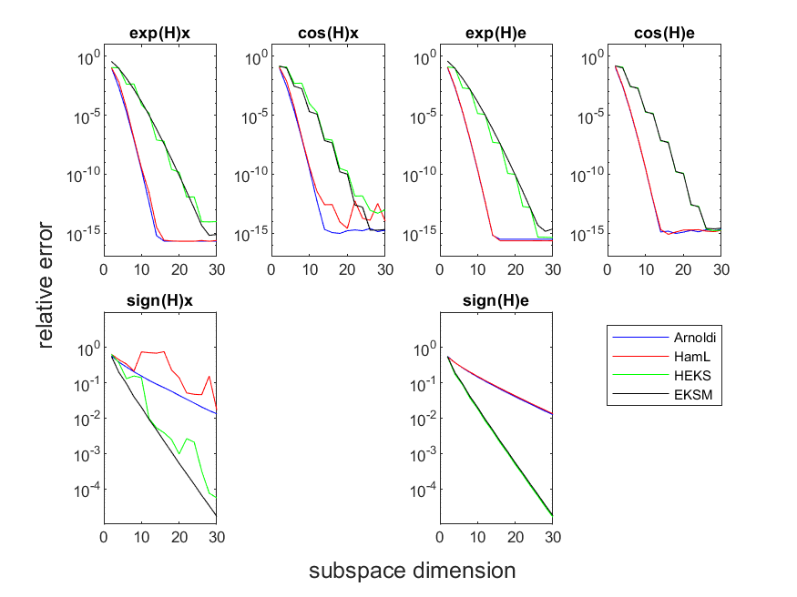
Figure 1: Diagonal Hamiltonian matrix $H_{1}=\operatorname{diag}(A,-A)$ with A = diag(logspace(-1,0,500));, two different choices of the starting vector x = randn(1000,1) and e = ones(1000,1)

In Fig. 1, the relative accuracy of all four methods is displayed, using a random starting vector $x$ (plots in the two leftmost columns) as well as a starting vector of all ones (plots in the two rightmost columns). The Hamiltonian Lanczos method and the Arnoldi method perform alike just as the HEKS algorithm and the EKS method. For the functions $\exp$ and $\cos$ the HEKS approximation makes significant progress only every other iteration step (that is, whenever the columns of $\widetilde{S}$ span $\mathcal{K}_{k,k-1}$). The same holds for the EKSM approximation of $\cos(H)x$ and $\cos(H)e$, but not for the approximation of $\exp(H)x$ and $\exp(H)e.$ The HEKS algorithm adds the vectors from $\mathcal{K}_{r,s}$ in a different order than EKSM: HEKS alternates between adding two vectors from $\mathcal{K}_{2k}(H,u)$ and adding two vectors from $\mathcal{K}_{2k}(H^{-1},H^{-1}u)$ , while EKSM alternates between adding one vector from $\mathcal{K}_{2k}(H,u)$ and adding one from $\mathcal{K}_{2k}(H^{-1},H^{-1}u)$ (for $u=x$ or $u=e$). Thus, the columns of $\widetilde{S}$ and $Q$ span the same subspace only every other step. Adding vectors from $\mathcal{K}_{2k}(H^{-1},H^{-1}u)$ does not seem to be relevant for the HEKS approximations $\exp(H)u$ and $\cos(H)u$ as well for the EKSM approximation of $\cos(H)u.$ For the EKSM approximation of $\exp(H)u$ some convergence progress can be observed in every iteration step, but the overall convergence is similar to that of the HEKS approximation. In summary, the use of an extended Krylov subspace does not improve the convergence for these examples compared to the approximations computed using the Arnoldi method or the Hamiltonian Lanczos method. The latter two methods converge about twice as fast as the first two.

But for the matrix sign function, the two methods based on the extended Krylov subspace converge faster than the other two. They do make progress in every iteration step. It is clearly beneficial to use an extended Krylov subspace here.

The HEKS algorithm requires $34$ matrix-vector-multiplications with $H$, $21$ linear solves with $H$ and $104$ scalar products to construct the $1000\times 30$ matrix $\widetilde{S}.$ In contrast, the ESKM requires $15$ matrix-vector-multiplications with $H$, $14$ linear solves with $H$ and $493$ scalar products. As $H$ in this example is diagonal, the linear solves and matrix-vector multiplications require less arithmetic operations than scalar products. Hence, the HEKS algorithm is faster than EKSM and requires less storage. Of course, the situation will change for more practically relevant examples with a more complex sparsity pattern. But it remains to note that there is a big difference in the number of scalar products to be performed, which is not due to the matrix structure but the difference of the short-term Lanczos-style and long-term Arnoldi-style recursions in the non-symmetric case.

7.2 Example 2

As a second example we use the Hamiltonian matrix $H_{2}=\left[\begin{smallmatrix}A&-G\\ -Q&-A^{T}\end{smallmatrix}\right]\in\mathbb{R}^{1998\times 1998}$ from Example 15 of the collection of benchmark examples for the numerical solution of continuous-time algebraic Riccati equations [6]. The matrix has a complex spectrum with real and imaginary parts between $-2$ and $2.$

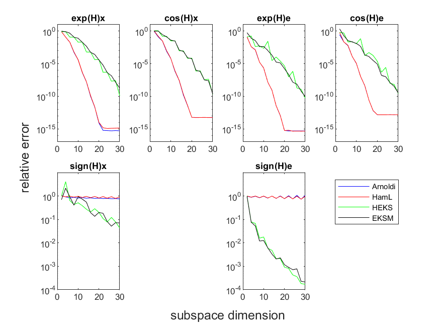
Figure 2: Hamiltonian matrix $H_{2}$, two different choices of the starting vector x = randn(1998,1) and e = ones(1998,1)

Fig. 2 provides the same information as in Fig. 1. Our findings from the first example are confirmed. The Hamiltonian Lanczos method and the Arnoldi method perform alike just as the HEKS algorithm and the EKS method. For the functions $\exp$ and $\cos$ the first two methods converge faster than the latter two. The use of the extended Krylov subspace does not result in faster convergence. But for the matrix sign function, the two method based on the extended Krylov subspace perform much better.

8 Concluding Remarks

The HEKS algorithm for computing a $J$-orthogonal basis of the extended Krylov subspace $\mathcal{K}_{r,s}$ (1.1) has been presented. Unlike the EKSM for generating an orthogonal basis of $\mathcal{K}_{r,r}$ it allows for short recurrences. The convergence analysis provide in [15] does not apply here as the field of values of a Hamiltonian matrix does not (strictly) lie in the right half-plane. Numerical experiments suggest that it may be useful to employ the HEKS algorithm for the approximation of the action of $f(H)$ on a vector $u$ for Hamiltonian matrices $H.$ The performance of the HEKS algorithm is similar to that of EKSM, but HEKS guarantees the structure-preserving projection of the Hamiltonian matrix which may be relevant for some applications.

Appendix A Derivation of the HEKS Algorithm

This section is devoted to deriving short recurrences for the HEKS algorithm. We will follow the idea sketched in Section 3. First $S_{1}\in\mathbb{R}^{2n\times 2}$ is constructed such that $S_{1}^{T}J_{n}S_{1}=J_{1}$ and the columns of $S_{1}$ span the same subspace as $\mathcal{K}_{2}(H,u_{1})$ (that is, $\operatorname{range}\{S_{1}\}=\mathcal{K}_{2}(H,u_{1})$). Here $H\in\mathbb{R}^{2n\times 2n}$ is the Hamiltonian matrix under consideration and $u_{1}\in\mathbb{R}^{2n}$ a given vector with $\|u_{1}\|_{2}=1$. Next $S_{2k}\in\mathbb{R}^{2n\times 4k}$ is constructed by extending $S_{2k-1}$ by two columns such that $S_{2k}^{T}J_{n}S_{2k}=J_{2k}$ and $\operatorname{range}\{S_{2k}\}=\mathcal{K}_{2k}(H,u_{1})+\mathcal{K}_{2k}(H^{-1},H^{-1}u_{1}).$ Finally, $S_{2k+1}\in\mathbb{R}^{2n\times 4k+2}$ is constructed by extending $S_{2k}$ by two columns such that $S_{2k+1}^{T}J_{n}S_{2k+1}=J_{2k+1}$ and $\operatorname{range}\{S_{2k+1}\}=\mathcal{K}_{2k+1}(H,u_{1})+\mathcal{K}_{2k}(H^{-1},H^{-1}u_{1}).$ In doing so, we will provide a proof that the projected matrices $H_{2k}$ and $H_{2k+1}$ as well as $J_{2k}^{T}S_{2k}^{T}J_{n}H^{-1}S_{2k}$ and $J_{2k+1}^{T}S_{2k+1}^{T}J_{n}H^{-1}S_{2k+1}$ are of the above given forms (4.3), (5.6) and (5.7), resp.. In particular, we will prove Theorem 4.1. The assumption in Theorem 4.1 that no breakdown occurs in particular implies that in the following all assumptions on nonzero parameters must hold.

A.1 Step 1: $\operatorname{range}\{S_{1}\}=\mathcal{K}_{2}(H,u_{1})$

As $u_{1}$ satisfies $\|u_{1}\|_{2}=1,$ there is nothing to do with the first vector in $\mathcal{K}_{2}(H,u_{1})$. The second vector $Hu_{1}$ needs to $J$-orthogonalized against $u_{1}.$ This is achieved by

(A.11) $$v_{1}=Hu_{1}/u_{1}^{T}J_{n}Hu_{1}=Hu_{1}/\vartheta_{1}$$

assuming that $\vartheta_{1}\neq 0.$ Thus, the matrix $S_{1}=[u_{1}\mid v_{1}]$ has $J$-orthogonal columns by construction

$$S_{1}^{T}J_{n}S_{1}=\begin{bmatrix}u_{1}^{T}J_{n}u_{1}&u_{1}^{T}J_{n}v_{1}\\ v_{1}^{T}J_{n}u_{1}&v_{1}^{T}J_{n}v_{1}\end{bmatrix}=\begin{bmatrix}0&1\\ -1&0\end{bmatrix}$$

as any vector is $J$-orthogonal to itself, $u_{1}^{T}J_{n}v_{1}=u_{1}^{T}J_{n}Hu_{1}/u_{1}^{T}J_{n}Hu_{1}=1$ and $v_{1}^{T}J_{n}u_{1}=(u_{1}^{T}J_{n}^{T}v_{1})^{T}=-(u_{1}^{T}J_{n}v_{1})^{T}.$

A.1.1 The projected matrix $H_{1}=J_{1}^{T}S_{1}^{T}J_{n}HS_{1}$

We will prove that

(A.12) $$H_{1}=J_{1}^{T}S_{1}^{T}J_{n}HS_{1}=\begin{bmatrix}-v_{1}^{T}J_{n}Hu_{1}&-v_{1}^{T}J_{n}Hv_{1}\\ u_{1}^{T}J_{n}Hu_{1}&u_{1}^{T}J_{n}Hv_{1}\end{bmatrix}=\begin{bmatrix}0&\alpha_{1}\\ \vartheta_{1}&0\end{bmatrix}$$

holds. Due to (A.11) we have $Hu_{1}=\vartheta_{1}v_{1}$ and thus

$$v_{1}^{T}J_{n}Hu_{1}=\vartheta_{1}\cdot v_{1}^{T}J_{n}v_{1}=0$$

as any vector is $J$-orthogonal to itself. The zero in position (2,2) follows from the zero in position $(1,1)$ as $H$ as well as $H_{1}$ is Hamiltonian (or by noting that $0=v_{1}^{T}J_{n}Hu_{1}=(v_{1}^{T}J_{n}H^{T}u_{1})^{T}=u_{1}^{T}(J_{n}H)^{T}v_{1}=u_{1}^{T}J_{n}Hv_{1}=0$).

A.1.2 The projected matrix $J_{1}^{T}S_{1}^{T}J_{n}H^{-1}S_{1}$

Making use of the fact that $H^{T}J_{n}H^{-1}=-J_{n}$ as $H$ is Hamiltonian ($(J_{n}H)^{T}=-H^{T}J_{n}=J_{n}H$), we have due to (A.11)

$$\vartheta_{1}\cdot v_{1}^{T}J_{n}H^{-1}u_{1}=(Hu_{1})^{T}J_{n}H^{-1}u_{1}=u_{1}^{T}H^{T}J_{n}H^{-1}u_{1}=-u_{1}^{T}J_{n}u_{1}=0.$$

This implies $u_{1}^{T}J_{n}H^{-1}v_{1}=0.$ Moreover, using (A.11) again

$$v_{1}^{T}J_{n}H^{-1}v_{1} =(Hu_{1})^{T}J_{n}H^{-1}(Hu_{1})/\vartheta_{1}^{2}=u_{1}^{T}H^{T}J_{n}u_{1}/\vartheta_{1}^{2}=-u_{1}^{T}J_{n}Hu_{1}/\vartheta_{1}^{2}=-1/\vartheta_{1}.$$

Thus

(A.13) $$J_{1}^{T}S_{1}^{T}J_{n}H^{-1}S_{1}=\begin{bmatrix}-v_{1}^{T}J_{n}H^{-1}u_{1}&-v_{1}^{T}J_{n}H^{-1}v_{1}\\ u_{1}^{T}J_{n}H^{-1}u_{1}&u_{1}^{T}J_{n}H^{-1}v_{1}\end{bmatrix}=\begin{bmatrix}0&1/\vartheta_{1}\\ f_{11}&0\end{bmatrix}.$$

A.2 Step 2: $\operatorname{range}\{S_{2}\}=\mathcal{K}_{2}(H,u_{1})+\mathcal{K}_{2}(H^{-1},H^{-1}u_{1})$

Now the first vector from the Krylov subspace $\mathcal{K}_{r}(H^{-1},H^{-1}u_{1})$ is added to the symplectic basis by $J$-orthogonalization $H^{-1}u_{1}$ against $u_{1}$ and $v_{1}.$ This is achieved by computing

$$w_{x}=(I-S_{1}J_{1}^{T}S_{1}^{T}J_{n})H^{-1}u_{1},$$

and normalizing $w_{x}$ to length 1, $x_{1}=w_{x}/\|w_{x}\|_{2}$. Next the second vector from $\mathcal{K}_{r}(H^{-1},H^{-1}u_{1})$ needs to be added to the symplectic basis. This can be accomplished by $J$-orthogonalizing $H^{-1}x_{1}$ against $u_{1}$ and $v_{1}$

$$w_{y} =(I-S_{1}J_{1}^{T}S_{1}^{T}J_{n})H^{-1}x_{1}$$

and making sure that $w_{y}$ is $J$-orthogonal against $x_{1}$ as well, $y_{1}=w_{y}/w_{y}^{T}Jx_{1}.$ Here we assume that $\|w_{x}\|_{2}\neq 0$ as well as $w_{y}^{T}Jx_{1}\neq 0.$

Collect the vectors into a matrix $S_{2}=[y_{1}\leavevmode\nobreak\ u_{1}\mid x_{1}\leavevmode\nobreak\ v_{1}]\in\mathbb{R}^{2n\times 4}.$ By construction the columns of $S_{2}$ are $J$-orthogonal, that is

(A.14) $$S_{2}^{T}J_{n}S_{2}=J_{2}$$

and

$$\operatorname{range}\{S_{2}\}=\mathcal{K}_{2}(H,u_{1})+\mathcal{K}_{2}(H^{-1},H^{-1}u_{1}).$$

Let us take a closer look at $w_{x}$ and $w_{y}.$ Making use of (A.13) we have

$$w_{x} =H^{-1}u_{1}-[v_{1}\leavevmode\nobreak\ -u_{1}]\begin{bmatrix}u_{1}^{T}J_{n}H^{-1}u_{1}\\ v_{1}^{T}J_{n}H^{-1}u_{1}\end{bmatrix}=H^{-1}u_{1}-[v_{1}\leavevmode\nobreak\ -u_{1}]\begin{bmatrix}f_{11}\\ 0\end{bmatrix}=H^{-1}u_{1}-f_{11}v_{1}.$$

Hence, with $\psi_{1}=\|w_{x}\|_{2}$ we have

(A.15) $$x_{1}=\left(H^{-1}u_{1}-f_{11}v_{1}\right)/\psi_{1},$$

where, as already stated above, $\psi_{1}\neq 0$ is assumed.

Next we turn our attention to $w_{y}.$ We will make use of the fact that $H^{-1}$ is Hamiltonian ($J_{n}H^{-1}=-H^{-T}J_{n}$) and $S_{2}^{T}J_{n}S_{2}=J_{2}.$ With (A.15) we see

(A.16) $$u_{1}^{T}J_{n}H^{-1}x_{1} =-(H^{-1}u_{1})^{T}J_{n}x_{1}=-(\psi_{1}x_{1}+f_{11}v_{1})^{T}J_{n}x_{1}=0.$$

Similarly, it follows with (A.11) that

(A.17) $$v_{1}^{T}J_{n}H^{-1}x_{1} =-(H^{-1}v_{1})^{T}J_{n}x_{1}=u_{1}^{T}J_{n}x_{1}/\vartheta_{1}=0.$$

Hence,

$$w_{y} =H^{-1}x_{1}-[v_{1}\leavevmode\nobreak\ -u_{1}]\begin{bmatrix}u_{1}^{T}J_{n}H^{-1}x_{1}\\ v_{1}^{T}J_{n}H^{-1}x_{1}\end{bmatrix}=H^{-1}x_{1}-[v_{1}\leavevmode\nobreak\ -u_{1}]\begin{bmatrix}0\\ 0\end{bmatrix}=H^{-1}x_{1},$$

and

$$y_{1}=H^{-1}x_{1}/\xi_{1},$$

where we assume that

(A.18) $$\xi_{1}=(H^{-1}x_{1})^{T}J_{n}x_{1}=x_{1}^{T}H^{-T}J_{n}x_{1}\neq 0.$$

Observe that

(A.19) $$\begin{split}\delta_{1}=y_{1}^{T}J_{n}Hy_{1}&=\frac{1}{\xi_{1}^{2}}x_{1}^{T}H^{-T}J_{n}HH^{-1}x_{1}=\frac{1}{\xi_{1}^{2}}x_{1}^{T}H^{-T}J_{n}x_{1}=\frac{1}{\xi_{1}}.\end{split}$$

Thus

(A.20) $$y_{1}=H^{-1}x_{1}/\xi_{1}=\delta_{1}H^{-1}x_{1}.$$

A.2.1 The projected matrix $H_{2}=J_{2}^{T}S_{2}^{T}J_{n}HS_{2}$

We will see that the zero structure of $H_{2}=J_{2}^{T}S_{2}^{T}J_{n}HS_{2}$ is given as follows:

(A.29) $$H_{2} =\left[\begin{array}[]{cc||cc}-x_{1}^{T}J_{n}Hy_{1}&-x_{1}^{T}J_{n}Hu_{1}&-x_{1}^{T}J_{n}Hx_{1}&-x_{1}^{T}J_{n}Hv_{1}\\ -v_{1}^{T}J_{n}Hy_{1}&-{\color[rgb]{0,0,1}v_{1}^{T}J_{n}Hu_{1}}&-v_{1}^{T}J_{n}Hx_{1}&-{\color[rgb]{0,0,1}v_{1}^{T}J_{n}Hv_{1}}\\ \hline\cr\hline\cr y_{1}^{T}J_{n}Hy_{1}&y_{1}^{T}J_{n}Hu_{1}&y_{1}^{T}J_{n}Hx_{1}&y_{1}^{T}J_{n}Hv_{1}\\ u_{1}^{T}J_{n}Hy_{1}&{\color[rgb]{0,0,1}u_{1}^{T}J_{n}Hu_{1}}&u_{1}^{T}J_{n}Hx_{1}&{\color[rgb]{0,0,1}u_{1}^{T}J_{n}Hv_{1}}\end{array}\right]=\left[\begin{array}[]{cc||cc}0&0&\lambda_{1}&\gamma_{1}\\ 0&{\color[rgb]{0,0,1}0}&\gamma_{1}&{\color[rgb]{0,0,1}\alpha_{1}}\\ \hline\cr\hline\cr\delta_{1}&0&0&0\\ 0&{\color[rgb]{0,0,1}\vartheta_{1}}&0&{\color[rgb]{0,0,1}0}\end{array}\right].$$

The entries at the positions $(2,2),(4,2),(2,4)$ and $(4,4)$ (denoted in blue in (A.29)) are the same as in (A.12). Due to $H$ and thus $H_{2}$ being Hamiltonian, we only need to prove the zero entries at the positions $(1,1),(1,2),(2,1)$ and $(3,2)$, the other zeros in (A.29) follow immediately.

Due to (A.11) we have $Hu_{1}=\vartheta_{1}v_{1}$. Thus, $x_{1}^{T}J_{n}Hu_{1}=\vartheta_{1}\cdot x_{1}^{T}J_{n}v_{1}=0$ and $y_{1}^{T}J_{n}Hu_{1}=\vartheta_{1}\cdot y_{1}^{T}J_{n}v_{1}=0$ due to (A.14). This gives the zero entries in the positions $(1,2)$ and $(3,2)$.

Due to (A.20) it follows with (A.14) for the entry $(2,1)$

$$v_{1}^{T}J_{n}Hy_{1} =\delta_{1}v_{1}^{T}J_{n}HH^{-1}x_{1}=\delta_{1}v_{1}^{T}J_{n}x_{1}=0.$$

Moreover, in a similar way for the entry $(1,1)$ we have

$$x_{1}^{T}J_{n}Hy_{1} =\delta_{1}x_{1}^{T}J_{n}HH^{-1}x_{1}=\delta_{1}x_{1}^{T}J_{n}x_{1}=0.$$

Hence, (A.29) holds.

A.2.2 The projected matrix $J_{2}^{T}S_{2}^{T}J_{n}H^{-1}S_{2}$

Some of the entries in $\tilde{H}_{2}=J_{2}^{T}S_{2}^{T}J_{n}H^{-1}S_{2}$ (denoted in blue) are already known from (A.13),

(A.34) $$\tilde{H}_{2} =\left[\begin{array}[]{cc|cc}-x_{1}^{T}J_{n}H^{-1}y_{1}&-x_{1}^{T}J_{n}H^{-1}u_{1}&-x_{1}^{T}J_{n}H^{-1}x_{1}&-x_{1}^{T}J_{n}H^{-1}v_{1}\\ -v_{1}^{T}J_{n}H^{-1}y_{1}&-{\color[rgb]{0,0,1}v_{1}^{T}J_{n}H^{-1}u_{1}}&-v_{1}^{T}J_{n}H^{-1}x_{1}&-{\color[rgb]{0,0,1}v_{1}^{T}J_{n}H^{-1}v_{1}}\\ \hline\cr y_{1}^{T}J_{n}H^{-1}y_{1}&y_{1}^{T}J_{n}H^{-1}u_{1}&y_{1}^{T}J_{n}H^{-1}x_{1}&y_{1}^{T}J_{n}H^{-1}v_{1}\\ u_{1}^{T}J_{n}H^{-1}y_{1}&{\color[rgb]{0,0,1}u_{1}^{T}J_{n}H^{-1}u_{1}}&u_{1}^{T}J_{n}H^{-1}x_{1}&{\color[rgb]{0,0,1}u_{1}^{T}J_{n}H^{-1}v_{1}}\end{array}\right]$$

(A.39) $$=\left[\begin{array}[]{cc|cc}0&0&1/\delta_{1}&0\\ 0&{\color[rgb]{0,0,1}0}&0&{\color[rgb]{0,0,1}1/\vartheta_{1}}\\ \hline\cr e_{11}&g_{11}&0&0\\ g_{11}&{\color[rgb]{0,0,1}f_{11}}&0&{\color[rgb]{0,0,1}0}\end{array}\right].$$

The entry in position $(1,3)$ follows from (A.18) and (A.19), while the zero entries in the positions $(1,2)$, $(1,4)$, $(2,3)$ and $(4,3)$ have already been proven in (A.16) and (A.17).

It remains to consider the entries at the positions $(3,3)$ and $(3,4)$. Using (A.20) and (A.11) leads to

$$y_{1}^{T}J_{n}H^{-1}x_{1} =\delta_{1}(H^{-1}x_{1})^{T}J_{n}(H^{-1}x_{1})=0,$$

$$y_{1}^{T}J_{n}H^{-1}v_{1} =y_{1}^{T}J_{n}u_{1}/\vartheta_{1}=0.$$

Hence, (A.39) holds.

A.3 Step 3: $\operatorname{range}\{S_{3}\}=\mathcal{K}_{4}(H,u_{1})+\mathcal{K}_{2}(H^{-1},H^{-1}u_{1})$

In this step the next two vectors $H^{2}u_{1}$ and $H^{3}u_{1}$ from $\mathcal{K}_{4}(H,u_{1})$ are added to the symplectic basis. We start by $J$-orthogonalizing $Hv_{1}$ against the columns of $S_{2}$

$$w_{u} =(I-S_{2}J_{2}^{T}S_{2}^{T}J_{n})Hv_{1}=Hv_{1}-[x_{1}\leavevmode\nobreak\ \leavevmode\nobreak\ v_{1}\leavevmode\nobreak\ \leavevmode\nobreak\ -y_{1}\leavevmode\nobreak\ \leavevmode\nobreak\ -u_{1}]\begin{bmatrix}y_{1}^{T}J_{n}Hv_{1}\\ u_{1}^{T}J_{n}Hv_{1}\\ x_{1}^{T}J_{n}Hv_{1}\\ v_{1}^{T}J_{n}Hv_{1}\end{bmatrix}$$

(A.40) $$=Hv_{1}-[x_{1}\leavevmode\nobreak\ \leavevmode\nobreak\ v_{1}\leavevmode\nobreak\ \leavevmode\nobreak\ -y_{1}\leavevmode\nobreak\ \leavevmode\nobreak\ -u_{1}]\begin{bmatrix}0\\ 0\\ -\gamma_{1}\\ -\alpha_{1}\end{bmatrix}=Hv_{1}-\gamma_{1}y_{1}-\alpha_{1}u_{1}$$

where (A.29) gives that the first two entries of the last vector are zero. Normalizing $w_{u}$ to length $1$ gives $u_{2}$

(A.41) $$u_{2}=w_{u}/\chi_{2},$$

where it is assumed that $\chi_{2}=\|w_{u}\|_{2}\neq 0.$

This step is finalized by $J$-orthogonalizing $Hu_{2}$ against the columns of $S_{2}$:

$$w_{v} =(I-S_{2}J_{2}^{T}S_{2}^{T}J_{n})Hu_{2}=Hu_{2}-[x_{1}\leavevmode\nobreak\ \leavevmode\nobreak\ v_{1}\leavevmode\nobreak\ \leavevmode\nobreak\ -y_{1}\leavevmode\nobreak\ \leavevmode\nobreak\ -u_{1}]\begin{bmatrix}y_{1}^{T}J_{n}Hu_{2}\\ u_{1}^{T}J_{n}Hu_{2}\\ x_{1}^{T}J_{n}Hu_{2}\\ v_{1}^{T}J_{n}Hu_{2}\end{bmatrix}.$$

All entries of the last vector are zero. The first two zeros follow as $H^{-T}J_{n}H=-J_{n}$ with (A.20) and (A.11):

$$y_{1}^{T}J_{n}Hu_{2}/\delta_{1} =(H^{-1}x_{1})^{T}J_{n}Hu_{2}=-x_{1}^{T}J_{n}u_{2}=0,$$

$$u_{1}^{T}J_{n}Hu_{2}/\vartheta_{1} =(H^{-1}v_{1})^{T}J_{n}Hu_{2}=-v_{1}^{T}J_{n}u_{2}=0$$

by construction of $u_{2}.$ The last zero follows as $H$ is Hamiltonian with (A.40),

$$v_{1}^{T}J_{n}Hu_{2} =v_{1}^{T}(J_{n}H)^{T}u_{2}=-(Hv_{1})^{T}J_{n}u_{2}=-(\chi_{2}u_{2}+\gamma_{1}y_{1}+\alpha_{1}u_{1})^{T}J_{n}u_{2}=0$$

again due to the construction of $u_{2}.$ With this and (A.15) we have for the next to last entry

$$\psi_{1}\cdot x_{1}^{T}J_{n}Hu_{2} =(H^{-1}u_{1}+f_{11}v_{1})^{T}J_{n}Hu_{2}=-u_{1}^{T}J_{n}u_{2}+f_{11}v_{1}^{T}J_{n}Hu_{2}=0.$$

Thus the expression for $w_{v}$ simplifies to

$$w_{v}=Hu_{2}.$$

Normalizing $w_{v}$ by $\vartheta_{2}=u_{2}^{T}J_{n}Hu_{2}$ to make sure it is $J$-orthogonal to $u_{2}$ as well yields

$$v_{2}=Hu_{2}/\vartheta_{2}.$$

Let

$$S_{3}=[y_{1}\leavevmode\nobreak\ u_{1}\leavevmode\nobreak\ u_{2}\mid x_{1}\leavevmode\nobreak\ v_{1}\leavevmode\nobreak\ v_{2}]\in\mathbb{R}^{2n\times 6}.$$

Then by construction

(A.42) $$S_{3}^{T}J_{n}S_{3}=J_{3}$$

and

$$\operatorname{range}\{S_{3}\}=\mathcal{K}_{4}(H,u_{1})+\mathcal{K}_{2}(H^{-1},H^{-1}u_{1}).$$

A.3.1 The projected matrix $H_{3}=J_{3}^{T}S_{3}^{T}J_{n}HS_{3}$

Some of the entries (denoted in blue) in $H_{3}=J_{3}^{T}S_{3}^{T}J_{n}HS_{3}$ are already known from (A.29)

(A.49) $$H_{3} ={\small\left[\begin{array}[]{c|cc||c|cc}{\color[rgb]{0,0,1}0}&{\color[rgb]{0,0,1}0}&-x_{1}^{T}J_{n}Hu_{2}&{\color[rgb]{0,0,1}\lambda_{1}}&{\color[rgb]{0,0,1}\gamma_{1}}&-x_{1}^{T}J_{n}Hv_{2}\\ \hline\cr{\color[rgb]{0,0,1}0}&{\color[rgb]{0,0,1}0}&-v_{1}^{T}J_{n}Hu_{2}&{\color[rgb]{0,0,1}\gamma_{1}}&{\color[rgb]{0,0,1}\alpha_{1}}&-v_{1}^{T}J_{n}Hv_{2}\\ -v_{2}^{T}J_{n}Hy_{1}&-v_{2}^{T}J_{n}Hu_{1}&-v_{2}^{T}J_{n}Hu_{2}&-v_{2}^{T}J_{n}Hx_{1}&-v_{2}^{T}J_{n}Hv_{1}&-v_{2}^{T}J_{n}Hv_{2}\\ \hline\cr\hline\cr{\color[rgb]{0,0,1}\delta_{1}}&{\color[rgb]{0,0,1}0}&y_{1}^{T}J_{n}Hu_{2}&{\color[rgb]{0,0,1}0}&{\color[rgb]{0,0,1}0}&y_{1}^{T}J_{n}Hv_{2}\\ \hline\cr{\color[rgb]{0,0,1}0}&{\color[rgb]{0,0,1}\vartheta_{1}}&u_{1}^{T}J_{n}Hu_{2}&{\color[rgb]{0,0,1}0}&{\color[rgb]{0,0,1}0}&u_{1}^{T}J_{n}Hv_{2}\\ u_{2}^{T}J_{n}Hy_{1}&u_{2}^{T}J_{n}Hu_{1}&u_{2}^{T}J_{n}Hu_{2}&u_{2}^{T}J_{n}Hx_{1}&u_{2}^{T}J_{n}Hv_{1}&u_{2}^{T}J_{n}Hv_{2}\end{array}\right]}$$

(A.56) $$=\left[\begin{array}[]{c|cc||c|cc}{\color[rgb]{0,0,1}0}&{\color[rgb]{0,0,1}0}&0&{\color[rgb]{0,0,1}\lambda_{1}}&{\color[rgb]{0,0,1}\gamma_{1}}&\mu_{2}\\ \hline\cr{\color[rgb]{0,0,1}0}&{\color[rgb]{0,0,1}0}&0&{\color[rgb]{0,0,1}\gamma_{1}}&{\color[rgb]{0,0,1}\alpha_{1}}&\beta_{2}\\ 0&0&0&\mu_{2}&\beta_{2}&\alpha_{2}\\ \hline\cr\hline\cr{\color[rgb]{0,0,1}\delta_{1}}&{\color[rgb]{0,0,1}0}&0&{\color[rgb]{0,0,1}0}&{\color[rgb]{0,0,1}0}&0\\ \hline\cr{\color[rgb]{0,0,1}0}&{\color[rgb]{0,0,1}\vartheta_{1}}&0&{\color[rgb]{0,0,1}0}&{\color[rgb]{0,0,1}0}&0\\ 0&0&\vartheta_{2}&0&0&0\end{array}\right].$$

The zeros in the third column (and hence the zeros in the last row) follow with $Hu_{2}=\vartheta_{2}v_{2}$ due to (A.42). Moreover, we have with (A.20) and (A.11)

$$v_{2}^{T}J_{n}Hy_{1} =\delta_{1}v_{2}^{T}J_{n}x_{1}=0,$$

$$v_{2}^{T}J_{n}Hu_{1} =\vartheta_{1}v_{2}^{T}J_{n}v_{1}=0$$

making again use of (A.42). Hence, (A.56) holds.

A.3.2 The projected matrix $J_{3}^{T}S_{3}^{T}J_{n}H^{-1}S_{3}$

Some of the entries in $\tilde{H}_{3}=J_{3}^{T}S_{3}^{T}J_{n}H^{-1}S_{3}$ (denoted in blue) are already known from (A.39)

(A.63) $$\tilde{H}_{3} ={\footnotesize\left[\begin{array}[]{ccc|ccc}{\color[rgb]{0,0,1}0}&{\color[rgb]{0,0,1}0}&-x_{1}^{T}J_{n}H^{-1}u_{2}&{\color[rgb]{0,0,1}1/\delta_{1}}&{\color[rgb]{0,0,1}0}&-x_{1}^{T}J_{n}H^{-1}v_{2}\\ {\color[rgb]{0,0,1}0}&{\color[rgb]{0,0,1}0}&-v_{1}^{T}J_{n}H^{-1}u_{2}&{\color[rgb]{0,0,1}0}&{\color[rgb]{0,0,1}1/\vartheta_{1}}&-v_{1}^{T}J_{n}H^{-1}v_{2}\\ -v_{2}^{T}J_{n}H^{-1}y_{1}&-v_{2}^{T}J_{n}H^{-1}u_{1}&-v_{2}^{T}J_{n}H^{-1}u_{2}&-v_{2}^{T}J_{n}H^{-1}x_{1}&-v_{2}^{T}J_{n}H^{-1}v_{1}&-v_{2}^{T}J_{n}H^{-1}v_{2}\\ \hline\cr{\color[rgb]{0,0,1}e_{11}}&{\color[rgb]{0,0,1}g_{11}}&y_{1}^{T}J_{n}H^{-1}u_{2}&{\color[rgb]{0,0,1}0}&{\color[rgb]{0,0,1}0}&y_{1}^{T}J_{n}H^{-1}v_{2}\\ {\color[rgb]{0,0,1}g_{11}}&{\color[rgb]{0,0,1}f_{11}}&u_{1}^{T}J_{n}H^{-1}u_{2}&0&0&u_{1}^{T}J_{n}H^{-1}v_{2}\\ u_{2}^{T}J_{n}H^{-1}y_{1}&u_{2}^{T}J_{n}H^{-1}u_{1}&u_{2}^{T}J_{n}H^{-1}u_{2}&u_{2}^{T}J_{n}H^{-1}x_{1}&u_{2}^{T}J_{n}H^{-1}v_{1}&u_{2}^{T}J_{n}H^{-1}v_{2}\end{array}\right]}$$

(A.70) $$=\left[\begin{array}[]{ccc|ccc}{\color[rgb]{0,0,1}0}&{\color[rgb]{0,0,1}0}&0&{\color[rgb]{0,0,1}1/\delta_{1}}&{\color[rgb]{0,0,1}0}&0\\ {\color[rgb]{0,0,1}0}&{\color[rgb]{0,0,1}0}&0&{\color[rgb]{0,0,1}0}&{\color[rgb]{0,0,1}1/\vartheta_{1}}&0\\ 0&0&0&0&0&1/\vartheta_{2}\\ \hline\cr{\color[rgb]{0,0,1}e_{11}}&{\color[rgb]{0,0,1}g_{11}}&g_{12}&{\color[rgb]{0,0,1}0}&{\color[rgb]{0,0,1}0}&0\\ {\color[rgb]{0,0,1}g_{11}}&{\color[rgb]{0,0,1}f_{11}}&0&{\color[rgb]{0,0,1}0}&{\color[rgb]{0,0,1}0}&0\\ g_{12}&0&f_{22}&0&0&0\end{array}\right].$$

It remains to show that the five entries $v_{2}^{T}J_{n}H^{-1}z$ for $z=x_{1},v_{1},y_{1},u_{1},u_{2}$ as well as the three entries $z^{T}J_{n}H^{-1}u_{2}$ for $z=v_{1},x_{1},u_{1}$ are zero. Moreover, we need to show that $-v_{2}^{T}J_{n}H^{-1}v_{2}=1/\vartheta_{2}.$

Most of these relations follow from $H^{T}J_{n}H^{-T}=-J_{n}$ and due to $Hu_{j}=\vartheta_{j}v_{j},j=1,2.$ Making use of (A.42) in the last equality of each equation we have

$$\vartheta_{1}\cdot v_{1}^{T}J_{n}H^{-1}u_{2} =u_{1}^{T}H^{T}J_{n}H^{-1}u_{2}=-u_{1}^{T}J_{n}u_{2}=0,$$

$$\vartheta_{2}\cdot v_{2}^{T}J_{n}H^{-1}v_{2} =u_{2}^{T}H^{T}J_{n}H^{-1}v_{2}=-u_{2}^{T}J_{n}v_{2}=-1,$$

and for $z=x_{1},v_{1},y_{1},u_{1},u_{2}$

$$\vartheta_{2}\cdot v_{2}^{T}J_{n}H^{-1}z =u_{2}^{T}H^{T}J_{n}H^{-1}z=-u_{2}^{T}J_{n}z=0.$$

Thus, $-v_{2}^{T}J_{n}H^{-1}v_{2}=1/\vartheta_{2}$ and the five entries in the $(1,1)$ (and the $(2,2)$) block of $\tilde{H}_{3}$ are zero.

The derivation of the final two zero entries needs a slightly more involved derivation. Due to (A.41), (A.42) and (A.39) we have

$$\chi_{2}\cdot x_{1}^{T}J_{n}H^{-1}u_{2} =x_{1}^{T}J_{n}H^{-1}(Hv_{1}-\gamma_{1}y_{1}-\alpha_{1}u_{1})$$

$$=x_{1}^{T}J_{n}v_{1}-\gamma_{1}x_{1}^{T}J_{n}H^{-1}y_{1}-\alpha_{1}x_{1}^{T}J_{n}H^{-1}u_{1}=0,$$

while due to $H^{-1}$ being Hamiltonian, (A.15) and (A.42) we get

$$u_{1}^{T}J_{n}H^{-1}u_{2}=(H^{-1}u_{1})^{T}J_{n}u_{2}=(\psi_{1}x_{1}+f_{11}v_{1})^{T}J_{n}u_{2}=0.$$

Hence, (A.70) holds.

A.4 Step 4: $\operatorname{range}\{S_{4}\}=\mathcal{K}_{4}(H,u_{1})+\mathcal{K}_{4}(H^{-1},H^{-1}u_{1})$

In this step the next two vectors $H^{-3}u_{1}$ and $H^{-4}u_{1}$ from $\mathcal{K}_{4}(H^{-1},H^{-1}u_{1})$ are added to the symplectic basis. We start by $J$-orthogonalizing $H^{-1}y_{1}$ against the columns of $S_{3}$

$$w_{x} =(I-S_{3}J_{3}^{T}S_{3}^{T}J_{n})H^{-1}y_{1}=H^{-1}y_{1}-[x_{1}\leavevmode\nobreak\ V_{2}\mid-y_{1}\leavevmode\nobreak\ -U_{2}]\begin{bmatrix}y_{1}^{T}J_{n}H^{-1}y_{1}\\ U_{2}^{T}J_{n}H^{-1}y_{1}\\ x_{1}^{T}J_{n}H^{-1}y_{1}\\ V_{2}^{T}J_{n}H^{-1}y_{1}\end{bmatrix}$$

$$=H^{-1}y_{1}-[x_{1}\leavevmode\nobreak\ V_{2}\mid-y_{1}\leavevmode\nobreak\ -U_{2}]\begin{bmatrix}e_{11}\\ g_{11}\\ g_{12}\\ 0\\ 0\\ 0\end{bmatrix}=H^{-1}y_{1}-e_{11}x_{1}-g_{11}v_{1}-g_{12}v_{2}$$

due to (A.70).

Normalizing $w_{x}$ to length $1$ gives

(A.71) $$x_{2}=w_{x}/\psi_{2},$$

where we assume that $\psi_{2}=\|w_{x}\|_{2}\neq 0.$

This step is finalized by $J$-orthogonalizing $H^{-1}x_{2}$ against the columns of $S_{3}$

(A.72) $$w_{y} =(I-S_{3}J_{3}^{T}S_{3}^{T}J_{n})H^{-1}x_{2}=H^{-1}x_{2}-[x_{1}\leavevmode\nobreak\ V_{2}\mid-y_{1}\leavevmode\nobreak\ -U_{2}]\begin{bmatrix}y_{1}^{T}J_{n}H^{-1}x_{2}\\ U_{2}^{T}J_{n}H^{-1}x_{2}\\ x_{1}^{T}J_{n}H^{-1}x_{2}\\ V_{2}^{T}J_{n}H^{-1}x_{2}\end{bmatrix}.$$

All entries $z^{T}J_{n}H^{-1}x_{2}=-(H^{-1}z)^{T}J_{n}x_{2}$ in the last vector are zero. As $Hu_{i}=\vartheta_{i}v_{i},$ $i=1,2,$ for the last two entries we have

$$\vartheta_{1}\cdot(H^{-1}v_{1})^{T}J_{n}x_{2} =u_{1}^{T}J_{n}x_{2}=0,$$

$$\vartheta_{2}\cdot(H^{-1}v_{2})^{T}J_{n}x_{2} =u_{2}^{T}J_{n}x_{2}=0$$

by construction of $x_{2}$ as a vector $J$-orthogonal to all columns of $S_{3}.$ Next, we use (A.71), (A.20) and (A.15) to see

$$(H^{-1}y_{1})^{T}J_{n}x_{2} =(\psi_{2}x_{2}-e_{11}x_{1}-g_{11}v_{1}-g_{12}v_{2})^{T}J_{n}x_{2}=0,$$

$$(H^{-1}x_{1})^{T}J_{n}x_{2} =\xi_{1}y_{1}^{T}J_{n}x_{2}=0,$$

$$(H^{-1}u_{1})^{T}J_{n}x_{2} =(\psi_{1}x_{1}-f_{11}v_{1})^{T}J_{n}x_{2}=0$$

again by construction of $x_{2}$ as a vector $J$-orthogonal to all columns of $S_{3}.$ With this and (A.41), it follows that

$$\chi_{2}\cdot(H^{-1}u_{2})^{T}J_{n}x_{2} =(v_{1}-\gamma_{1}H^{-1}y_{1}-\alpha_{1}H^{-1}u_{1})^{T}J_{n}x_{2}=0.$$

Thus,

$$y_{2}=H^{-1}x_{2}/\xi_{2},$$

where we assume that

(A.73) $$\xi_{2}=(H^{-1}x_{2})^{T}J_{n}x_{2}=x_{2}^{T}H^{-T}J_{n}x_{2}\neq 0.$$

With the same argument as in (A.19) we see that

$$\delta_{2}=y_{2}^{T}J_{n}Hy_{2}=\frac{1}{\xi_{2}^{2}}(H^{-1}x_{2})^{T}J_{n}HH^{-1}x_{2}=\frac{1}{\xi_{2}}.$$

Thus

(A.74) $$y_{2}=H^{-1}x_{2}/\xi_{2}=\delta_{2}H^{-1}x_{2}.$$

Let

$$S_{4}=[y_{2}\leavevmode\nobreak\ y_{1}\leavevmode\nobreak\ u_{1}\leavevmode\nobreak\ u_{2}\mid x_{2}\leavevmode\nobreak\ x_{1}\leavevmode\nobreak\ v_{1}\leavevmode\nobreak\ v_{2}]\in\mathbb{R}^{2n\times 8}.$$

Then by construction

(A.75) $$S_{4}^{T}J_{n}S_{4}=J_{4}$$

and

$$\operatorname{range}\{S_{4}\}=\mathcal{K}_{4}(H,u_{1})+\mathcal{K}_{4}(H^{-1},H^{-1}u_{1}).$$

A.4.1 The projected matrix $H_{4}=J_{4}^{T}S_{4}^{T}J_{n}HS_{4}$

Some of the entries in $H_{4}=J_{4}^{T}S_{4}^{T}J_{n}HS_{4}$ (denoted in blue) are already known from (A.56)

$$H_{4}={\footnotesize\left[\begin{array}[]{cc|cc||cc|cc}-x_{2}^{T}J_{n}Hy_{2}&-x_{2}^{T}J_{n}Hy_{1}&-x_{2}^{T}J_{n}Hu_{1}&-x_{2}^{T}J_{n}Hu_{2}&-x_{2}^{T}J_{n}Hx_{2}&-x_{2}^{T}J_{n}Hx_{1}&-x_{2}^{T}J_{n}Hv_{1}&-x_{2}^{T}J_{n}Hv_{2}\\ -x_{1}^{T}J_{n}Hy_{2}&{\color[rgb]{0,0,1}0}&{\color[rgb]{0,0,1}0}&{\color[rgb]{0,0,1}0}&-x_{1}^{T}J_{n}Hx_{2}&{\color[rgb]{0,0,1}\lambda_{1}}&{\color[rgb]{0,0,1}\gamma_{1}}&{\color[rgb]{0,0,1}\mu_{2}}\\ \hline\cr-v_{1}^{T}J_{n}Hy_{2}&{\color[rgb]{0,0,1}0}&{\color[rgb]{0,0,1}0}&{\color[rgb]{0,0,1}0}&-v_{1}^{T}J_{n}Hx_{2}&{\color[rgb]{0,0,1}\gamma_{1}}&{\color[rgb]{0,0,1}\alpha_{1}}&{\color[rgb]{0,0,1}\beta_{2}}\\ -v_{2}^{T}J_{n}Hy_{2}&{\color[rgb]{0,0,1}0}&{\color[rgb]{0,0,1}0}&{\color[rgb]{0,0,1}0}&-v_{2}^{T}J_{n}Hx_{2}&{\color[rgb]{0,0,1}\mu_{2}}&{\color[rgb]{0,0,1}\beta_{2}}&{\color[rgb]{0,0,1}\alpha_{2}}\\ \hline\cr\hline\cr y_{2}^{T}J_{n}Hy_{2}&y_{2}^{T}J_{n}Hy_{1}&y_{2}^{T}J_{n}Hu_{1}&y_{2}^{T}J_{n}Hu_{2}&y_{2}^{T}J_{n}Hx_{2}&y_{2}^{T}J_{n}Hx_{1}&y_{2}^{T}J_{n}Hv_{1}&y_{2}^{T}J_{n}Hv_{2}\\ y_{1}^{T}J_{n}Hy_{2}&{\color[rgb]{0,0,1}\delta_{1}}&{\color[rgb]{0,0,1}0}&{\color[rgb]{0,0,1}0}&y_{1}^{T}J_{n}Hx_{2}&{\color[rgb]{0,0,1}0}&{\color[rgb]{0,0,1}0}&{\color[rgb]{0,0,1}0}\\ \hline\cr u_{1}^{T}J_{n}Hy_{2}&{\color[rgb]{0,0,1}0}&{\color[rgb]{0,0,1}\vartheta_{1}}&{\color[rgb]{0,0,1}0}&u_{1}^{T}J_{n}Hx_{2}&{\color[rgb]{0,0,1}0}&{\color[rgb]{0,0,1}0}&{\color[rgb]{0,0,1}0}\\ u_{2}^{T}J_{n}Hy_{2}&{\color[rgb]{0,0,1}0}&{\color[rgb]{0,0,1}0}&{\color[rgb]{0,0,1}\vartheta_{2}}&u_{2}^{T}J_{n}Hx_{2}&{\color[rgb]{0,0,1}0}&{\color[rgb]{0,0,1}0}&{\color[rgb]{0,0,1}0}\end{array}\right]}$$

We will show that

(A.84) $$H_{4}=\left[\begin{array}[]{cc|cc||cc|cc}0&0&0&0&\lambda_{2}&0&0&\gamma_{2}\\ 0&{\color[rgb]{0,0,1}0}&{\color[rgb]{0,0,1}0}&{\color[rgb]{0,0,1}0}&0&{\color[rgb]{0,0,1}\lambda_{1}}&{\color[rgb]{0,0,1}\gamma_{1}}&{\color[rgb]{0,0,1}\mu_{2}}\\ \hline\cr 0&{\color[rgb]{0,0,1}0}&{\color[rgb]{0,0,1}0}&{\color[rgb]{0,0,1}0}&0&{\color[rgb]{0,0,1}\gamma_{1}}&{\color[rgb]{0,0,1}\alpha_{1}}&{\color[rgb]{0,0,1}\beta_{2}}\\ 0&{\color[rgb]{0,0,1}0}&{\color[rgb]{0,0,1}0}&{\color[rgb]{0,0,1}0}&\gamma_{2}&{\color[rgb]{0,0,1}\mu_{2}}&{\color[rgb]{0,0,1}\beta_{2}}&{\color[rgb]{0,0,1}\alpha_{2}}\\ \hline\cr\hline\cr\delta_{2}&0&0&0&0&0&0&0\\ 0&{\color[rgb]{0,0,1}\delta_{1}}&{\color[rgb]{0,0,1}0}&{\color[rgb]{0,0,1}0}&0&{\color[rgb]{0,0,1}0}&{\color[rgb]{0,0,1}0}&{\color[rgb]{0,0,1}0}\\ \hline\cr 0&{\color[rgb]{0,0,1}0}&{\color[rgb]{0,0,1}\vartheta_{1}}&{\color[rgb]{0,0,1}0}&0&{\color[rgb]{0,0,1}0}&{\color[rgb]{0,0,1}0}&{\color[rgb]{0,0,1}0}\\ 0&{\color[rgb]{0,0,1}0}&{\color[rgb]{0,0,1}0}&{\color[rgb]{0,0,1}\vartheta_{2}}&0&{\color[rgb]{0,0,1}0}&{\color[rgb]{0,0,1}0}&{\color[rgb]{0,0,1}0}\end{array}\right].$$

Let us consider the entries in the first column of (A.84). We make use of (A.74) and obtain

$$z^{T}J_{n}Hy_{2}=\delta_{2}z^{T}J_{n}x_{2}.$$

For $z=x_{1},x_{2},v_{1},v_{2},y_{1},u_{1},u_{2}$ we have $z^{T}J_{n}x_{2}=0$ due to (A.75), while, $y_{2}^{T}J_{n}x_{2}=1.$ Thus $y_{2}^{T}J_{n}Hy_{2}=\delta_{2}.$ Moreover, the other 7 entries in the first column are zero. This implies that the other 7 entries in the fifth row are zero as well.

For the entries $x_{2}^{T}J_{n}Hz$ for $z=y_{1},u_{1},u_{2},$ in the first row we note that

$$\psi_{2}\cdot x_{2}^{T}J_{n}Hz =(H^{-1}y_{1}-e_{11}x_{1}-g_{11}v_{1}-g_{12}v_{2})^{T}J_{n}Hz=-y_{1}^{T}J_{n}z-(e_{11}x_{1}+g_{11}v_{1}+g_{12}v_{2})^{T}J_{n}Hz=0$$

due to (A.71), (A.75) and (A.56). These zeros imply zeros in the positions $(6,5),(7,5)$ and $(8,5).$

It remains to consider the two entries at the positions $(1,6)$ and $(1,7)$. With (A.15) it follows that

$$\psi_{1}\cdot x_{2}^{T}J_{n}Hx_{1} =x_{2}^{T}J_{n}H(H^{-1}u_{1}-f_{11}v_{1})=x_{2}^{T}J_{n}u_{1}-f_{11}x_{2}^{T}J_{n}Hv_{1}=-f_{11}x_{2}^{T}J_{n}Hv_{1}$$

due to (A.75). Thus, the entry at position $(1,6)$ is zero if and only if the entry at position $(1,7)$ is zero. For the entry at position $(1,7)$ we have with (A.41) and (A.40)

$$x_{2}^{T}J_{n}Hv_{1} =x_{2}^{T}J_{n}(\chi_{2}u_{2}+\gamma_{1}y_{1}\alpha_{1}u_{1})=0$$

due to (A.75). Hence, (A.84) holds.

A.4.2 The projected matrix $J_{4}^{T}S_{4}^{T}J_{n}H^{-1}S_{4}$

Some of the entries in $\tilde{H}_{4}=J_{4}^{T}S_{4}^{T}J_{n}H^{-1}S_{4}$ (denoted in blue) are already known from (A.70),

(A.93) $${\tiny\left[\begin{array}[]{cccc|cccc}-x_{2}^{T}J_{n}H^{-1}y_{2}&{\color[rgb]{1,0,0}0}&{\color[rgb]{1,0,0}0}&{\color[rgb]{1,0,0}0}&-x_{2}^{T}J_{n}H^{-1}x_{2}&{\color[rgb]{1,0,0}0}&{\color[rgb]{1,0,0}0}&{\color[rgb]{1,0,0}0}\\ -x_{1}^{T}J_{n}H^{-1}y_{2}&{\color[rgb]{0,0,1}0}&{\color[rgb]{0,0,1}0}&{\color[rgb]{0,0,1}0}&{\color[rgb]{1,0,0}0}&{\color[rgb]{0,0,1}1/\delta_{1}}&{\color[rgb]{0,0,1}0}&{\color[rgb]{0,0,1}0}\\ -v_{1}^{T}J_{n}H^{-1}y_{2}&{\color[rgb]{0,0,1}0}&{\color[rgb]{0,0,1}0}&{\color[rgb]{0,0,1}0}&{\color[rgb]{1,0,0}0}&{\color[rgb]{0,0,1}0}&{\color[rgb]{0,0,1}1/\vartheta_{1}}&{\color[rgb]{0,0,1}0}\\ -v_{2}^{T}J_{n}H^{-1}y_{2}&{\color[rgb]{0,0,1}0}&{\color[rgb]{0,0,1}0}&{\color[rgb]{0,0,1}0}&{\color[rgb]{1,0,0}0}&{\color[rgb]{0,0,1}0}&{\color[rgb]{0,0,1}0}&{\color[rgb]{0,0,1}1/\vartheta_{2}}\\ \hline\cr y_{2}^{T}J_{n}H^{-1}y_{2}&y_{2}^{T}J_{n}H^{-1}y_{1}&y_{2}^{T}J_{n}H^{-1}u_{1}&y_{2}^{T}J_{n}H^{-1}u_{2}&y_{2}^{T}J_{n}H^{-1}x_{2}&y_{2}^{T}J_{n}H^{-1}x_{1}&y_{2}^{T}J_{n}H^{-1}v_{1}&y_{2}^{T}J_{n}H^{-1}v_{2}\\ y_{1}^{T}J_{n}H^{-1}y_{2}&{\color[rgb]{0,0,1}e_{11}}&{\color[rgb]{0,0,1}g_{11}}&{\color[rgb]{0,0,1}g_{12}}&{\color[rgb]{1,0,0}0}&{\color[rgb]{0,0,1}0}&{\color[rgb]{0,0,1}0}&{\color[rgb]{0,0,1}0}\\ u_{1}^{T}J_{n}H^{-1}y_{2}&{\color[rgb]{0,0,1}g_{11}}&{\color[rgb]{0,0,1}f_{11}}&{\color[rgb]{0,0,1}0}&{\color[rgb]{1,0,0}0}&{\color[rgb]{0,0,1}0}&{\color[rgb]{0,0,1}0}&{\color[rgb]{0,0,1}0}\\ u_{2}^{T}J_{n}H^{-1}y_{2}&{\color[rgb]{0,0,1}g_{12}}&{\color[rgb]{0,0,1}0}&{\color[rgb]{0,0,1}f_{22}}&{\color[rgb]{1,0,0}0}&{\color[rgb]{0,0,1}0}&{\color[rgb]{0,0,1}0}&{\color[rgb]{0,0,1}0}\end{array}\right]}$$

(A.102) $$=\left[\begin{array}[]{cc|cc||cc|cc}0&{\color[rgb]{1,0,0}0}&{\color[rgb]{1,0,0}0}&{\color[rgb]{1,0,0}0}&1/\delta_{2}&{\color[rgb]{1,0,0}0}&{\color[rgb]{1,0,0}0}&{\color[rgb]{1,0,0}0}\\ 0&{\color[rgb]{0,0,1}0}&{\color[rgb]{0,0,1}0}&{\color[rgb]{0,0,1}0}&{\color[rgb]{1,0,0}0}&{\color[rgb]{0,0,1}1/\delta_{1}}&{\color[rgb]{0,0,1}0}&{\color[rgb]{0,0,1}0}\\ \hline\cr 0&{\color[rgb]{0,0,1}0}&{\color[rgb]{0,0,1}0}&{\color[rgb]{0,0,1}0}&{\color[rgb]{1,0,0}0}&{\color[rgb]{0,0,1}0}&{\color[rgb]{0,0,1}1/\vartheta_{1}}&{\color[rgb]{0,0,1}0}\\ 0&{\color[rgb]{0,0,1}0}&{\color[rgb]{0,0,1}0}&{\color[rgb]{0,0,1}0}&{\color[rgb]{1,0,0}0}&{\color[rgb]{0,0,1}0}&{\color[rgb]{0,0,1}0}&{\color[rgb]{0,0,1}1/\vartheta_{2}}\\ \hline\cr\hline\cr e_{22}&e_{12}&g_{12}&g_{22}&0&0&0&0\\ e_{12}&{\color[rgb]{0,0,1}e_{11}}&{\color[rgb]{0,0,1}g_{11}}&{\color[rgb]{0,0,1}g_{12}}&{\color[rgb]{1,0,0}0}&{\color[rgb]{0,0,1}0}&{\color[rgb]{0,0,1}0}&{\color[rgb]{0,0,1}0}\\ \hline\cr g_{12}&{\color[rgb]{0,0,1}g_{11}}&{\color[rgb]{0,0,1}f_{11}}&{\color[rgb]{0,0,1}0}&{\color[rgb]{1,0,0}0}&{\color[rgb]{0,0,1}0}&{\color[rgb]{0,0,1}0}&{\color[rgb]{0,0,1}0}\\ g_{22}&{\color[rgb]{0,0,1}g_{12}}&{\color[rgb]{0,0,1}0}&{\color[rgb]{0,0,1}f_{22}}&{\color[rgb]{1,0,0}0}&{\color[rgb]{0,0,1}0}&{\color[rgb]{0,0,1}0}&{\color[rgb]{0,0,1}0}\end{array}\right].$$

In addition, most of the ones in the 5th column (denoted in red) and hence in the first row are known from the derivations concerning (A.72).

Let us consider the remaining entries in the first row. As $H^{-1}$ is Hamiltonian and due to (A.73), we have

$$x_{2}^{T}J_{n}H^{-1}x_{2} =x_{2}^{T}(J_{n}H^{-1})^{T}x_{2}=-(H^{-1}x_{2})^{T}J_{n}x_{2}=-\xi_{2}=-1/\delta_{2}.$$

Due to (A.74) and (A.75) it follows that

$$\xi_{2}\cdot y_{2}^{T}J_{n}H^{-1}x_{2} =y_{2}^{T}J_{n}y_{2}=0.$$

Finally, we consider the three remaining entries in the first column,

$$z^{T}J_{n}H^{-1}y_{2}=-(H^{-1}z)^{T}J_{n}y_{2}$$

for $z=x_{1},v_{1},v_{2}.$ Due to $\vartheta_{i}H^{-1}v_{i}=u_{i}$ for $i=1,2,$ we obtain with (A.75)

$$\vartheta_{i}\cdot(H^{-1}v_{i})^{T}J_{n}y_{2}=u_{i}^{T}J_{n}y_{2}=0,$$

while with (A.20) we have

$$\delta_{1}\cdot(H^{-1}x_{1})^{T}J_{n}y_{2}=y_{1}^{T}J_{n}y_{2}=0.$$

Hence, (A.102) holds.

A.5 Step 5: $\operatorname{range}\{S_{5}\}=\mathcal{K}_{6}(H,u_{1})+\mathcal{K}_{4}(H^{-1},H^{-1}u_{1})$ and Step 6: $\operatorname{range}\{S_{6}\}=\mathcal{K}_{6}(H,u_{1})+\mathcal{K}_{6}(H^{-1},H^{-1}u_{1})$

We refrain from stating Steps 5 and 6 explicitly even so $u_{2}$ and $x_{2}$ are not displaying the general form of $u_{k}$ and $x_{k}$. This can only be seen from $u_{3}$ and $x_{3}$ which would be derived in Steps 5 and 6. As the derivations which lead to $u_{3}$ and $x_{3}$ are the same as in the general case for deriving $u_{k+1}$ and $x_{k+1},$ we directly proceed to the general case assuming that Algorithm 1 holds up to step $k.$

A.6 Step 2k+1: $\operatorname{range}\{S_{2k+1}\}=\mathcal{K}_{2k+2}(H,u_{1})+\mathcal{K}_{2k}(H^{-1},H^{-1}u_{1})$

Assume that we have constructed

$$S_{2k}=[y_{k}\leavevmode\nobreak\ \cdots\leavevmode\nobreak\ y_{1}\leavevmode\nobreak\ u_{1}\leavevmode\nobreak\ \cdots\leavevmode\nobreak\ u_{k}\mid x_{k}\leavevmode\nobreak\ \cdots\leavevmode\nobreak\ x_{1}\leavevmode\nobreak\ v_{1}\leavevmode\nobreak\ \cdots\leavevmode\nobreak\ v_{k}]=[Y_{k}\leavevmode\nobreak\ U_{k}\mid X_{k}\leavevmode\nobreak\ V_{k}]\in\mathbb{R}^{2n\times 4k}$$

such that $S_{2k}^{T}JnS_{2k}=J_{2k}$,

$$H_{2k} =J_{2k}^{T}S_{2k}^{T}J_{n}HS_{2k}={\small\begin{bmatrix}-X_{k}^{T}J_{n}HY_{k}&-X_{k}^{T}J_{n}HU_{k}&-X_{k}^{T}J_{n}HX_{k}&-X_{k}^{T}J_{n}HV_{k}\\ -V_{k}^{T}J_{n}HY_{k}&-V_{k}^{T}J_{n}HU_{k}&-V_{k}^{T}J_{n}HX_{k}&-V_{k}^{T}J_{n}HV_{k}\\ Y_{k}^{T}J_{n}HY_{k}&Y_{k}^{T}J_{n}HU_{k}&Y_{k}^{T}J_{n}HX_{k}&Y_{k}^{T}J_{n}HV_{k}\\ U_{k}^{T}J_{n}HY_{k}&U_{k}^{T}J_{n}HU_{k}&U_{k}^{T}J_{n}HX_{k}&U_{k}^{T}J_{n}HV_{k}\end{bmatrix}}$$

(A.103) $$=\begin{bmatrix}0&0&\Lambda_{k}&B_{kk}\\ 0&0&B_{kk}^{T}&T_{k}\\ \Delta_{k}&0&0&0\\ 0&\Theta_{k}&0&0\end{bmatrix}$$

as in (4.3) ($r=s=k$),

$$\tilde{H}_{2k} =J_{2k}^{T}S_{2k}^{T}J_{n}H^{-1}S_{2k}={\small\begin{bmatrix}-X_{k}^{T}J_{n}H^{-1}Y_{k}&-X_{k}^{T}J_{n}H^{-1}U_{k}&-X_{k}^{T}J_{n}H^{-1}X_{k}&-X_{k}^{T}J_{n}H^{-1}V_{k}\\ -V_{k}^{T}J_{n}H^{-1}Y_{k}&-V_{k}^{T}J_{n}H^{-1}U_{k}&-V_{k}^{T}J_{n}H^{-1}X_{k}&-V_{k}^{T}J_{n}H^{-1}V_{k}\\ Y_{k}^{T}J_{n}H^{-1}Y_{k}&Y_{k}^{T}J_{n}H^{-1}U_{k}&Y_{k}^{T}J_{n}H^{-1}X_{k}&Y_{k}^{T}J_{n}H^{-1}V_{k}\\ U_{k}^{T}J_{n}H^{-1}Y_{k}&U_{k}^{T}J_{n}H^{-1}U_{k}&U_{k}^{T}J_{n}H^{-1}X_{k}&U_{k}^{T}J_{n}H^{-1}V_{k}\end{bmatrix}}$$

(A.104) $$=\begin{bmatrix}0&0&\Delta_{k}^{-1}&0\\ 0&0&0&\Theta_{k}^{-1}\\ E_{k}&G_{kk}&0&0\\ G_{kk}^{T}&F_{k}&0&0\end{bmatrix}$$

as in (5.6) and

$$\operatorname{range}\{S_{2k}\}=\mathcal{K}_{{2k}}(H,u_{1})+\mathcal{K}_{{2k}}(H^{-1},H^{-1}u_{1}).$$

The computational steps can be found in Algorithm 1.

In this step the next two vectors $H^{2k}u_{1}$ and $H^{2k+1}u_{1}$ from $\mathcal{K}_{2k+2}(H,u_{1})$ are added to the symplectic basis. Due to the previous construction, this is achieved by first considering $Hv_{k}$. $J$-orthogonalizing $Hv_{k}$ against the columns of $S_{2k}$ yields

$$w_{u} =(I-S_{2k}J_{2}^{T}S_{2k}^{T}J_{n})Hv_{k}=Hv_{k}-[X_{k}\leavevmode\nobreak\ \leavevmode\nobreak\ V_{k}\leavevmode\nobreak\ \leavevmode\nobreak\ -Y_{k}\leavevmode\nobreak\ \leavevmode\nobreak\ -U_{k}]\begin{bmatrix}Y_{k}^{T}J_{n}Hv_{k}\\ U_{k}^{T}J_{n}Hv_{k}\\ X_{k}^{T}J_{n}Hv_{k}\\ V_{k}^{T}J_{n}Hv_{k}\end{bmatrix}$$

$$=Hv_{k}-\gamma_{k}y_{k}-\mu_{k}y_{k-1}-\beta_{k}u_{k-1}-\alpha_{k}u_{k}$$

as due to (A.103)

$$Y_{k}^{T}J_{n}Hv_{k} =0, U_{k}^{T}J_{n}Hv_{k}=0,$$

$$X_{k}^{T}J_{n}Hv_{k} =\begin{bmatrix}-\gamma_{k}\\ -\mu_{k}\\ 0\\ \vdots\\ 0\end{bmatrix}, V_{k}^{T}J_{n}Hv_{k}=\begin{bmatrix}0\\ \vdots\\ 0\\ -\beta_{k}\\ -\alpha_{k}\end{bmatrix}.$$

Normalizing $w_{u}$ to length $1$ gives

(A.105) $$u_{k+1}=w_{u}/\chi_{k+1},$$

where it is assumed that $\chi_{k+1}=\|w_{u}\|_{2}\neq 0.$

This step is finalized by $J$-orthogonalizing $Hu_{k+1}$ against the columns of $S_{2k}$

$$w_{v} =(I-S_{2k}J_{2k}^{T}S_{2k}^{T}J_{n})Hu_{k+1}=Hu_{k+1}-[X_{k}\leavevmode\nobreak\ \leavevmode\nobreak\ V_{k}\leavevmode\nobreak\ \leavevmode\nobreak\ -Y_{k}\leavevmode\nobreak\ \leavevmode\nobreak\ -U_{k}]\begin{bmatrix}Y_{k}^{T}J_{n}Hu_{k+1}\\ U_{k}^{T}J_{n}Hu_{k+1}\\ X_{k}^{T}J_{n}Hu_{k+1}\\ V_{k}^{T}J_{n}Hu_{k+1}\end{bmatrix}.$$

All entries of the last vector are zero. The zeros in the first two blocks $Y_{k}^{T}J_{n}Hu_{k+1}$ and $U_{k}^{T}J_{n}Hu_{k+1}$ can be seen by using $y_{j}=\delta_{j}H^{-1}x_{j}$ and $u_{j}=\vartheta_{j}H^{-1}v_{j}$ for $j=1,\ldots,k$ as well as $H^{-T}J_{n}H=-J_{n}$:

$$y_{j}^{T}J_{n}Hu_{k+1}/\delta_{j} =(H^{-1}x_{j})^{T}J_{n}Hu_{k+1}=-x_{j}^{T}J_{n}u_{k+1}=0,$$

$$u_{j}^{T}J_{n}Hu_{k+1}/\vartheta_{j} =(H^{-1}v_{j})^{T}J_{n}Hu_{k+1}=-v_{j}^{T}J_{n}u_{k+1}=0,$$

due to the construction of $u_{k+1}$ as $J$-orthogonal against all columns of $S_{2k}.$

The zeros in the last block $V_{k}^{T}J_{n}Hv_{k}$ follow as $H$ is Hamiltonian and with

$$\chi_{j}u_{j}=Hv_{j}-\gamma_{j}y_{j}-\mu_{j}y_{j-1}-\beta_{j}u_{j-1}-\alpha_{j}u_{j}$$

for $j=1,\ldots,k,$ (where we set $\beta_{1}=\mu_{1}=0$ and $y_{0}=u_{0}=0$)

$$v_{j}^{T}J_{n}Hu_{k+1} =v_{j}^{T}(J_{n}H)^{T}u_{k+1}=-(Hv_{j})^{T}J_{n}u_{k+1}$$

(A.106) $$=-(\chi_{j}u_{j}+\gamma_{j}y_{j}+\mu_{j}y_{j-1}+\beta_{j}u_{j-1}+\alpha_{j}u_{j})^{T}J_{n}u_{k+1}=0,$$

again due to the construction of $u_{k+1}$ as $J$-orthogonal against all columns of $S_{2k}.$

With this we can show that the entries of the next to last block $X_{k}^{T}J_{n}Hv_{k}$ are all zero. First, with $\psi_{1}x_{1}=H^{-1}u_{1}-f_{11}v_{1}$ and $H^{-T}J_{n}H=-J_{n}$ we have

$$\psi_{1}\cdot x_{1}^{T}J_{n}Hu_{k+1} =(H^{-1}u_{1}-f_{11}v_{1})^{T}J_{n}Hu_{k+1}=u_{1}^{T}H^{-T}J_{n}Hu_{k+1}-f_{11}v_{1}J_{n}Hu_{k+1}$$

(A.107) $$=-u_{1}^{T}J_{n}u_{k+1}-f_{11}v_{1}J_{n}Hu_{k+1}=0$$

due to the construction of $u_{k+1}$ as $J$-orthogonal against all columns of $S_{2k}$ and due to (A.106). Next, we use

(A.108) $$\psi_{j+1}x_{j+1}=H^{-1}y_{j}-e_{jj}x_{j}-e_{j-1,j}x_{j-1}-g_{jj}v_{j}-g_{j1,j+1}v_{j+1}$$

for $j=1,\ldots,k-1$ (where we set $e_{01}=0$ and $x_{0}=0$, see Lines 16 and 29 of Algorithm 1) for the other entries of the next to last block

$$\psi_{j+1}\cdot x_{j+1}^{T}J_{n}Hu_{k+1} =-(e_{jj}x_{j}+e_{j-1,j}x_{j-1}+g_{jj}v_{j}+g_{j,j+1}v_{j+1})^{T}J_{n}Hu_{k+1}+y_{j}^{T}H^{-T}J_{n}Hu_{k+1}$$

$$=-(e_{jj}x_{j}+e_{j-1,j}x_{j-1})^{T}J_{n}Hu_{k+1}-y_{j}^{T}J_{n}u_{k+1}$$

as $v_{j}^{T}J_{n}Hu_{k+1}=0$ due to (A.106). Clearly, $y_{j}^{T}J_{n}u_{k+1}=0$ by construction of $u_{k+1}.$ Thus, it remains to consider

$$\psi_{j+1}\cdot x_{j+1}^{T}J_{n}Hu_{k+1} =-(e_{jj}x_{j}+e_{j-1,j}x_{j-1})^{T}J_{n}Hu_{k+1}.$$

For $j=1$ we have with $x_{0}=0$ and (A.107) that $\psi_{2}\cdot x_{2}^{T}J_{n}Hu_{k+1}=0.$ With this, we get $\psi_{3}\cdot x_{3}^{T}J_{n}Hu_{k+1}=0,$ and, continuing in this fashion,

$$\psi_{j+1}\cdot x_{j+1}^{T}J_{n}Hu_{k+1} =0.$$

Thus the expression for $w_{v}$ simplifies to

$$w_{v}=Hu_{k+1}.$$

Normalizing $w_{v}$ by $\vartheta_{k+1}=u_{k+1}^{T}J_{n}Hu_{k+1}$ to make sure it is $J$-orthogonal to $u_{k+1}$ yields

(A.109) $$v_{k+1}=Hu_{k+1}/\vartheta_{k+1}.$$

Let $S_{2k+1}=[y_{k}\leavevmode\nobreak\ \cdots\leavevmode\nobreak\ y_{1}\leavevmode\nobreak\ u_{1}\leavevmode\nobreak\ \cdots\leavevmode\nobreak\ u_{k+1}\mid x_{k}\leavevmode\nobreak\ \cdots\leavevmode\nobreak\ x_{1}\leavevmode\nobreak\ v_{1}\leavevmode\nobreak\ \cdots\leavevmode\nobreak\ v_{k+1}]=[Y_{k}\leavevmode\nobreak\ U_{k+1}\mid X_{k}\leavevmode\nobreak\ V_{k+1}]\in\mathbb{R}^{2n\times 4k+2}.$ Then by construction

(A.110) $$S_{2k+1}^{T}J_{n}S_{2k+1}=J_{2k+1}$$

and $\operatorname{range}\{S_{2k+1}\}=\mathcal{K}_{2k+2}(H,u_{1})+\mathcal{K}_{2k}(H^{-1},H^{-1}u_{1}).$

A.6.1 The projected matrix $H_{2k+1}=J_{2k+1}^{T}S_{2k+1}^{T}J_{n}HS_{2k+1}$

Most of the entries in $H_{2k+1}=J_{2k+1}^{T}S_{2k+1}^{T}J_{n}HS_{2k+1}$ (denoted in blue) are already known from $H_{2k}$ (A.103)

(A.117) $$H_{2k+1} ={\tiny\left[\begin{array}[]{c|cc||c|cc}{\color[rgb]{0,0,1}0}&{\color[rgb]{0,0,1}0}&-X_{k}^{T}J_{n}Hu_{k+1}&{\color[rgb]{0,0,1}\Lambda_{k}}&{\color[rgb]{0,0,1}B_{kk}}&-X_{k}^{T}J_{n}Hv_{k+1}\\ \hline\cr{\color[rgb]{0,0,1}0}&{\color[rgb]{0,0,1}0}&-V_{k}^{T}J_{n}Hu_{k+1}&{\color[rgb]{0,0,1}B_{kk}}^{T}&{\color[rgb]{0,0,1}T_{k}}&-V_{k}^{T}J_{n}Hv_{k+1}\\ -v_{k+1}^{T}J_{n}HY_{k}&-v_{k+1}^{T}J_{n}HU_{k}&-v_{k+1}^{T}J_{n}Hu_{k+1}&-v_{k+1}^{T}J_{n}HX_{k}&-v_{k+1}^{T}J_{n}HV_{k}&-v_{k+1}^{T}J_{n}Hv_{k+1}\\ \hline\cr\hline\cr{\color[rgb]{0,0,1}\Delta_{k}}&{\color[rgb]{0,0,1}0}&Y_{k}^{T}J_{n}Hu_{k+1}&{\color[rgb]{0,0,1}0}&{\color[rgb]{0,0,1}0}&Y_{k}^{T}J_{n}Hv_{k+1}\\ \hline\cr{\color[rgb]{0,0,1}0}&{\color[rgb]{0,0,1}\Theta_{k}}&U_{k}^{T}J_{n}Hu_{k+1}&{\color[rgb]{0,0,1}0}&{\color[rgb]{0,0,1}0}&U_{k}^{T}J_{n}Hv_{k+1}\\ u_{k+1}^{T}J_{n}HY_{k}&u_{k+1}^{T}J_{n}HU_{k}&u_{k+1}^{T}J_{n}Hu_{k+1}&u_{k+1}^{T}J_{n}HX_{k}&u_{k+1}^{T}J_{n}HV_{k}&u_{k+1}^{T}J_{n}Hv_{k+1}\end{array}\right]}$$

(A.128) $$=\left[\begin{array}[]{c|cc||c|cc}{\color[rgb]{0,0,1}0}&{\color[rgb]{0,0,1}0}&0&{\color[rgb]{0,0,1}\Lambda_{k}}&{\color[rgb]{0,0,1}B_{kk}}&\begin{smallmatrix}\mu_{k}\\ 0\\ \vdots\\ 0\end{smallmatrix}\\ \hline\cr{\color[rgb]{0,0,1}0}&{\color[rgb]{0,0,1}0}&0&{\color[rgb]{0,0,1}B_{kk}}^{T}&{\color[rgb]{0,0,1}T_{k}}&\begin{smallmatrix}0\\ \vdots\\ 0\\ \beta_{k+1}\end{smallmatrix}\\ 0&0&0&\begin{smallmatrix}\mu_{k}&0&\cdots&0\end{smallmatrix}&\begin{smallmatrix}0&\cdots&0&\beta_{k+1}\end{smallmatrix}&\alpha_{k+1}\\ \hline\cr\hline\cr{\color[rgb]{0,0,1}\Delta_{k}}&{\color[rgb]{0,0,1}0}&0&{\color[rgb]{0,0,1}0}&{\color[rgb]{0,0,1}0}&0\\ \hline\cr{\color[rgb]{0,0,1}0}&{\color[rgb]{0,0,1}\Theta_{k}}&0&{\color[rgb]{0,0,1}0}&{\color[rgb]{0,0,1}0}&0\\ 0&0&\vartheta_{k+1}&0&0&0\end{array}\right]=\left[\begin{array}[]{c|c||c|c}0&0&\Lambda_{k}&B_{k,k+1}\\ \hline\cr 0&0&B_{k,k+1}^{T}&T_{k+1}\\ \hline\cr\hline\cr\Delta_{k}&0&0&0\\ \hline\cr 0&\Theta_{k+1}&0&0\end{array}\right].$$

The zeros in the third column (and hence in the last row) follow due to $Hu_{k+1}=\vartheta_{k+1}v_{k+1}$ and (A.110). The zeros in the first block $v_{k+1}^{T}J_{n}HY_{k}$ of the third row follow due to $Hy_{j}=\delta_{j}x_{j},$ for $j=1,\ldots,k,$ the ones in the second block $v_{k+1}^{T}J_{n}HU_{k}$ due to $Hu_{j}=\vartheta_{j}v_{j},$ $j=1,\ldots,k.$ This also implies the zeros in the last row of the fourth and fifth block.

Moreover, we obtain

$$v_{k+1}^{T}J_{n}HV_{k-1}=0$$

from

(A.129) $$\chi_{j+1}u_{j+1}=Hv_{j}-\gamma_{j}y_{j}-\mu_{j}y_{j-1}-\beta_{j}u_{j-1}-\alpha_{j}u_{j}$$

for $j=1,\ldots,k-1$ (where we set $\beta_{0}=\mu_{0}=0$ and $u_{0}=y_{0}=0,$ see Lines 11 and 24 in Algorithm 1) as

$$v_{k+1}^{T}J_{n}Hv_{j} =v_{k+1}^{T}J_{n}(\psi_{j+1}u_{j+1}+\gamma_{j}y_{j}+\mu_{j}y_{j-1}+\beta_{j}u_{j-1}+\alpha_{j}u_{j})=0$$

due to the construction of $v_{k+1}$ as $J$-orthogonal against all columns of $S_{2k}.$ With this, $\psi_{1}x_{1}=H^{-1}u_{1}-f_{11}v_{1}$ and the recurrence for $x_{j}$ as in (A.108), we observe that

$$v_{k+1}^{T}J_{n}HX_{k-1}=0$$

holds. This can be seen step by step. Due to (A.110) and $v_{k+1}^{T}J_{n}HV_{k-1}=0,$ we have

$$\psi_{1}v_{k+1}^{T}J_{n}Hx_{1} =v_{k+1}^{T}J_{n}H(H^{-1}u_{1}-f_{11}v_{1})=v_{k+1}^{T}J_{n}u_{1}-f_{11}v_{k+1}^{T}J_{n}Hv_{1}=0,$$

and with this and (A.71) we have further

$$\psi_{2}v_{k+1}^{T}J_{n}Hx_{2} =-v_{k+1}^{T}J_{n}y_{1}-e_{11}v_{k+1}^{T}J_{n}Hx_{1}-g_{11}v_{k+1}^{T}J_{n}Hv_{1}-g_{12}v_{k+1}^{T}J_{n}Hv_{2}=0.$$

In this fashion we continue with the expression for $x_{j+1}$ as in Line 30 of Algorithm 1 to obtain for $j=2,\ldots,k-2$

$$\psi_{j+1}v_{k+1}^{T}J_{n}Hx_{j+1} =-v_{k+1}^{T}J_{n}y_{j}-e_{jj}v_{k+1}^{T}J_{n}Hx_{j}-e_{j-1,j}v_{k+1}^{T}J_{n}Hx_{j-1}$$

$$\qquad-g_{jj}v_{k+1}^{T}J_{n}Hv_{j+1}-g_{j,j+1}v_{k+1}^{T}J_{n}Hv_{j}=0.$$

Hence, (A.128) holds.

A.6.2 The projected matrix $J_{2k+1}^{T}S_{2k+1}^{T}J_{n}H^{-1}S_{2k+1}$

Most of the entries in

$$\tilde{H}_{2k+1}=J_{2k+1}^{T}S_{2k+1}^{T}J_{n}H^{-1}S_{2k+1}$$

(denoted in blue) are already known from (A.6)

(A.136) $$\tilde{H}_{2k+1} ={\tiny\left[\begin{array}[]{ccc|ccc}{\color[rgb]{0,0,1}0}&{\color[rgb]{0,0,1}0}&-X_{k}^{T}J_{n}H^{-1}u_{k+1}&{\color[rgb]{0,0,1}\Delta_{k}^{-1}}&{\color[rgb]{0,0,1}0}&-X_{k}^{T}J_{n}H^{-1}v_{k+1}\\ {\color[rgb]{0,0,1}0}&{\color[rgb]{0,0,1}0}&-V_{k}^{T}J_{n}H^{-1}u_{k+1}&{\color[rgb]{0,0,1}0}&{\color[rgb]{0,0,1}\Theta_{k}}^{-1}&-V_{k}^{T}J_{n}H^{-1}v_{k+1}\\ -v_{k+1}^{T}J_{n}H^{-1}Y_{k}&-v_{k+1}^{T}J_{n}H^{-1}U_{k}&-v_{k+1}^{T}J_{n}H^{-1}u_{k+1}&-v_{k+1}^{T}J_{n}H^{-1}X_{k}&-v_{k+1}^{T}J_{n}H^{-1}V_{k}&-v_{k+1}^{T}J_{n}H^{-1}v_{k+1}\\ \hline\cr{\color[rgb]{0,0,1}E_{k}}&{\color[rgb]{0,0,1}G_{k}}&Y_{k}^{T}J_{n}H^{-1}u_{k+1}&{\color[rgb]{0,0,1}0}&{\color[rgb]{0,0,1}0}&Y_{k}^{T}J_{n}H^{-1}v_{k+1}\\ {\color[rgb]{0,0,1}G_{k}}^{T}&{\color[rgb]{0,0,1}F_{k}}&U_{k}^{T}J_{n}H^{-1}u_{k+1}&{\color[rgb]{0,0,1}0}&{\color[rgb]{0,0,1}0}&U_{k}^{T}J_{n}H^{-1}v_{k+1}\\ u_{k+1}^{T}J_{n}H^{-1}Y_{k}&u_{k+1}^{T}J_{n}H^{-1}U_{k}&u_{k+1}^{T}J_{n}H^{-1}u_{k+1}&u_{k+1}^{T}J_{n}H^{-1}X_{k}&u_{k+1}^{T}J_{n}H^{-1}V_{k}&u_{k+1}^{T}J_{n}H^{-1}v_{k+1}\end{array}\right]}$$

(A.147) $$=\left[\begin{array}[]{ccc|ccc}{\color[rgb]{0,0,1}0}&{\color[rgb]{0,0,1}0}&0&{\color[rgb]{0,0,1}\Delta_{k}^{-1}}&{\color[rgb]{0,0,1}0}&0\\ {\color[rgb]{0,0,1}0}&{\color[rgb]{0,0,1}0}&0&{\color[rgb]{0,0,1}0}&{\color[rgb]{0,0,1}\Theta_{k}}^{-1}&0\\ 0&0&0&0&0&1/\vartheta_{k+1}\\ \hline\cr{\color[rgb]{0,0,1}E_{k}}&{\color[rgb]{0,0,1}G_{k}}&\begin{smallmatrix}g_{k,k+1}\\ 0\\ \vdots\\ 0\end{smallmatrix}&{\color[rgb]{0,0,1}0}&{\color[rgb]{0,0,1}0}&0\\ {\color[rgb]{0,0,1}G_{k}}^{T}&{\color[rgb]{0,0,1}F_{k}}&0&{\color[rgb]{0,0,1}0}&{\color[rgb]{0,0,1}0}&0\\ \begin{smallmatrix}g_{k,k+1}&0&\cdots&0\end{smallmatrix}&0&f_{k+1,k+1}&0&0&0\end{array}\right]=\left[\begin{array}[]{cc|cc}0&0&\Delta_{k}^{-1}&0\\ 0&0&0&\Theta_{k+1}^{-1}\\ \hline\cr E_{k}&G_{k,k+1}&0&0\\ G_{k,k+1}^{T}&F_{k+1}&0&0\end{array}\right]$$

With (A.109) and $H^{-T}J_{n}H=-J_{n},$ we see that the entries $v_{k+1}^{T}J_{n}H^{-1}z$ in the third block row are zeros (despite the last entry)

(A.148) $$\vartheta_{1}\cdot v_{k+1}^{T}J_{n}H^{-1}z=u_{k+1}^{T}H^{T}J_{n}H^{-1}z=-u_{k+1}^{T}J_{n}z=0$$

for $z\in\{y_{1},\ldots,y_{k},u_{1},\ldots,u_{k+1},x_{1},\ldots,x_{k},v_{1}.\ldots,v_{k}\}$ due to the construction of $u_{k+1}$ as $J$-orthogonal to all columns of $S_{2k}.$ This implies the zeros in the last column of (A.147). For the last entry we have

$$-\vartheta_{k+1}\cdot v_{k+1}^{T}J_{n}H^{-1}v_{k+1}=-u_{k+1}^{T}H^{T}J_{n}H^{-1}v_{k+1}=u_{k+1}^{T}J_{n}v_{k+1}=1.$$

Thus, $-v_{k+1}^{T}J_{n}H^{-1}v_{k+1}=1/\vartheta_{k+1}.$

With (A.105) the entries in the upper part of the third column (as well as the entries in the fourth and fifth block of the last row) are zero as

$$\chi_{k+1}z^{T}J_{n}H^{-1}u_{k+1} =z^{T}J_{n}H^{-1}(Hv_{k}-\gamma_{k}y_{k}-\mu_{k}y_{k-1}-\beta_{k}u_{k-1}-\alpha_{k}u_{k})$$

$$=z^{T}J_{n}v_{k}-z^{T}J_{n}H^{-1}(\gamma_{k}y_{k}+\mu_{k}y_{k-1}+\beta_{k}u_{k-1}+\alpha_{k}u_{k})=0$$

for $z\in\{x_{1},\ldots,x_{k},v_{1},\ldots,v_{k}\}$ due to (A.148) and (A.6).

The entries in $Y_{k-1}^{T}J_{n}H^{-1}u_{k+1}$ are zero as $H^{-1}$ is Hamiltonian and (A.108) yield

(A.149) $$\begin{split}y_{j}^{T}J_{n}H^{-1}u_{k+1}&=-(H^{-1}y_{j})^{T}J_{n}u_{k+1}\\ &=-(\psi_{j+1}x_{j+1}-e_{jj}x_{j}-e_{j-1,j}x_{j-1}-g_{jj}v_{j}-g_{j,j+1}v_{j+1})^{T}J_{n}u_{k+1}=0\end{split}$$

for $j=1,\ldots,k-1$ due to the construction of $u_{k+1}$ as $J$-orthogonal to all columns of $S_{2k}.$

With this, we can show in a recursive manner that the entries in

$$U_{k-1}^{T}J_{n}H^{-1}u_{k+1}=-(H^{-1}U_{k-1})^{T}J_{n}u_{k+1}$$

are zero by making use of $\chi_{1}u_{1}=\psi_{1}x_{1}-f_{11}v_{1}$ and (A.129). First we obtain

(A.150) $$\chi_{1}\cdot(H^{-1}u_{1})^{T}J_{n}u_{k+1} =(\psi_{1}x_{1}-f_{11}v_{1})^{T}J_{n}u_{k+1}=0$$

due to the construction of $u_{k+1}$ as $J$-orthogonal to all columns of $S_{2k}.$ Next we observe

$$\chi_{2}\cdot(H^{-1}u_{2})^{T}J_{n}u_{k+1} =(v_{1}-\gamma_{1}H^{-1}y_{1}-\alpha_{1}H^{-1}u_{1})^{T}J_{n}u_{k+1}=0,$$

where the first term is zero as $u_{k+1}$ is $J$-orthogonal to $v_{1},$ the second one due to (A.149) and the third term due to (A.150). Continuing in this fashion, we have

$$\chi_{j}\cdot(H^{-1}u_{j})^{T}J_{n}u_{k+1} =(v_{j-1}-\gamma_{j-1}H^{-1}y_{j-1}-\mu_{j-1}H^{-1}y_{j-2})^{T}J_{n}u_{k+1}$$

$$\qquad-(\beta_{j-2}H^{-1}u_{j-2}+\alpha_{j-1}H^{-1}u_{j-1})^{T}J_{n}u_{k+1}=0$$

where the first term is zero as $u_{k+1}$ is $J$-orthogonal to $v_{j-1},$ the second and third one due to (A.149), and the fourth and fifth term due to the preceding observations.

Hence, (A.147) holds.

A.7 Step 2k+2: $\operatorname{range}\{S_{2k+2}\}=\mathcal{K}_{2k+2}(H,u_{1})+\mathcal{K}_{2k+2}(H^{-1},H^{-1}u_{1})$

Assume that we have constructed $S_{2k+1}=[Y_{k}\leavevmode\nobreak\ \leavevmode\nobreak\ U_{k+1}\mid X_{k}\leavevmode\nobreak\ \leavevmode\nobreak\ V_{k+1}]\in\mathbb{R}^{2n\times 4k+2}$ as in the previous section.

The two vectors $H^{-(2k+1)}u_{1}$ and $H^{-(2k+2)}u_{1}$ from $\mathcal{K}_{2k+2}(H^{-1},H^{-1}u_{1})$ are added to the symplectic basis. Due to the previous construction, this is achieved by constructing $x_{k+1}$ from $H^{-1}y_{k}$ and $y_{k+1}$ from $H^{-1}x_{k+1}.$ First $H^{-1}y_{k}$ is $J$-orthogonalized against the columns of $S_{2k+1}$:

$$w_{x} =(I-S_{2k+1}J_{2k+1}^{T}S_{2k+1}^{T}J_{n})H^{-1}y_{k}=H^{-1}y_{k}-[X_{k}\leavevmode\nobreak\ \leavevmode\nobreak\ V_{k+1}\leavevmode\nobreak\ \leavevmode\nobreak\ -Y_{k}\leavevmode\nobreak\ \leavevmode\nobreak\ -U_{k+1}]\begin{bmatrix}Y_{k}^{T}J_{n}H^{-1}y_{k}\\ U_{k+1}^{T}J_{n}H^{-1}y_{k}\\ X_{k}^{T}J_{n}H^{-1}y_{k}\\ V_{k+1}^{T}J_{n}H^{-1}y_{k}\end{bmatrix}$$

$$=H^{-1}y_{k}-e_{kk}x_{k}-e_{k-1,k}x_{k-1}-g_{kk}v_{k}-g_{k,k+1}v_{k+1}$$

due to (A.147). Normalizing $w_{x}$ to length $1$ gives

(A.151) $$x_{k+1}=w_{x}/\psi_{k+1},$$

where we assume that $\psi_{k+1}=\|w_{x}\|_{2}\neq 0.$

This step is finalized by $J$-orthogonalizing $H^{-1}x_{k+1}$ against the columns of $S_{2k+1}$:

$$w_{y} =(I-S_{2k+1}J_{2k+1}^{T}S_{2k+1}^{T}J_{n})H^{-1}x_{k+1}=H^{-1}x_{k+1}-[X_{k}\leavevmode\nobreak\ V_{k+1}\mid-Y_{k}\leavevmode\nobreak\ -U_{k+1}]\begin{bmatrix}Y_{k}^{T}J_{n}H^{-1}x_{k+1}\\ U_{k+1}^{T}J_{n}H^{-1}x_{k+1}\\ X_{k}^{T}J_{n}H^{-1}x_{k+1}\\ V_{k+1}^{T}J_{n}H^{-1}x_{k+1}\end{bmatrix}.$$

All entries $z^{T}J_{n}H^{-1}x_{k+1}=-(H^{-1}z)^{T}J_{n}x_{k+1}$ in the last vector are zero. In order to see this, let us first consider $z=v_{j},j=1,\ldots,k+1.$ Due to $\vartheta_{j}v_{j}=Hu_{j}$, we have immediately

$$(H^{-1}v_{j})^{T}J_{n}x_{k+1}=-u_{j}^{T}J_{n}x_{k+1}/\vartheta_{j}=0.$$

Next, we consider $z=x_{j},j=1,\ldots,k,$ and make use of $\xi_{j}y_{j}=H^{-1}x_{j}$ to obtain

$$(H^{-1}x_{j})^{T}J_{n}x_{k+1}=\zeta_{j}y_{j}^{T}J_{n}x_{k+1}=0.$$

Rewriting (A.108) in terms of $H^{-1}y_{j}$, the case $z=y_{j},j=1,\ldots,k$ yields

$$(H^{-1}y_{j})^{T}J_{n}x_{k+1} =(\psi_{j}x_{j}-e_{j-1,j-1}x_{j-1}-g_{j-1,j-1}v_{j-1}-g_{j-1,j}v_{j})^{T}J_{n}x_{k+1}=0.$$

Finally, for $z=u_{j}$ we obtain from (A.15)

$$(H^{-1}u_{1})^{T}J_{n}x_{k+1}=(\psi_{1}x_{1}-f_{11}v_{1})^{T}J_{n}x_{k+1}=0,$$

from (A.41)

$$(H^{-1}u_{2})^{T}J_{n}x_{k+1}=(v_{1}+\gamma_{1}H^{-1}y_{1}+\alpha_{1}H^{-1}u_{1})^{T}J_{n}x_{k+1}/\chi_{2}=0,$$

and from (A.105)

$$(H^{-1}u_{j+1})^{T}J_{n}x_{k+1} =(v_{j}+\gamma_{j}H^{-1}y_{j}+\mu_{j}y_{j-1}+\beta_{j}u_{j-1}+\alpha_{j}H^{-1}u_{j})^{T}J_{n}x_{k+1}/\chi_{j+1}=0$$

for $j=2,\ldots,k.$

Thus,

(A.152) $$y_{k+1}=H^{-1}x_{k+1}/\xi_{k+1}$$

where we assume that

$$\xi_{k+1}=(H^{-1}x_{k+1})^{T}J_{n}x_{k+1}=x_{k+1}^{T}H^{-T}J_{n}x_{k+1}\neq 0.$$

With the same argument as in (A.19) we see that

$$\delta_{k+1}=-\frac{1}{\xi_{k+1}}.$$

Let $S_{2k+2}=[y_{k+1}\leavevmode\nobreak\ Y_{k}\leavevmode\nobreak\ u_{k+1}\mid x_{k+1}\leavevmode\nobreak\ X_{k}\leavevmode\nobreak\ V_{k+1}]\in\mathbb{R}^{2n\times 4k+4}.$ Then by construction $S_{2k+2}^{T}J_{n}S_{2k+2}=J_{2k+2}$ and $\operatorname{range}\{S_{2k+2}\}=\mathcal{K}_{2k+2}(H,u_{1})+\mathcal{K}_{2k+2}(H^{-1},H^{-1}u_{1}).$

A.7.1 The projected matrix $H_{2k+2}=J_{2k+2}^{T}S_{2k+2}^{T}J_{n}HS_{2k+2}$

Most of the entries in $H_{2k+2}=J_{2k+2}^{T}S_{2k+2}^{T}J_{n}HS_{2k+2}$ (denoted in blue) are already known from (A.128)

(A.159) $${\footnotesize\left[\begin{array}[]{cc|c||cc|cc}-x_{k+1}^{T}J_{n}Hy_{k+1}&-x_{k+1}^{T}J_{n}HY_{k}&-x_{k+1}^{T}J_{n}HU_{k+1}&-x_{k+1}^{T}J_{n}Hx_{k+1}&-x_{k+1}^{T}J_{n}HX_{k}&-x_{k+1}^{T}J_{n}HV_{k+1}\\ -X_{k}^{T}J_{n}Hy_{k+1}&{\color[rgb]{0,0,1}0}&{\color[rgb]{0,0,1}0}&-X_{k}^{T}J_{n}Hx_{k+1}&{\color[rgb]{0,0,1}\Lambda_{k}}&{\color[rgb]{0,0,1}B_{k,k+1}}\\ \hline\cr-V_{k+1}^{T}J_{n}Hy_{k+1}&{\color[rgb]{0,0,1}0}&{\color[rgb]{0,0,1}0}&-V_{k+1}^{T}J_{n}Hx_{k+1}&{\color[rgb]{0,0,1}B_{k,k+1}}^{T}&{\color[rgb]{0,0,1}T_{k+1}}\\ \hline\cr\hline\cr y_{k+1}^{T}J_{n}Hy_{k+1}&y_{k+1}^{T}J_{n}HY_{k}&y_{k+1}^{T}J_{n}HU_{k+1}&y_{k+1}^{T}J_{n}Hx_{k+1}&y_{k+1}^{T}J_{n}HX_{k}&y_{k+1}^{T}J_{n}HV_{k+1}\\ Y_{k}^{T}J_{n}Hy_{k+1}&{\color[rgb]{0,0,1}\Delta_{k}}&{\color[rgb]{0,0,1}0}&Y_{k}^{T}J_{n}Hx_{k+1}&{\color[rgb]{0,0,1}0}&{\color[rgb]{0,0,1}0}\\ \hline\cr U_{k+1}^{T}J_{n}Hy_{k+1}&{\color[rgb]{0,0,1}0}&{\color[rgb]{0,0,1}\Theta_{k+1}}&U_{k+1}^{T}J_{n}Hx_{k+1}&{\color[rgb]{0,0,1}0}&{\color[rgb]{0,0,1}0}\end{array}\right]}$$

(A.170) $$=\left[\begin{array}[]{cc|c||cc|c}0&0&0&\lambda_{k+1}&0&\begin{smallmatrix}0&\cdots&0&\gamma_{k+1}\end{smallmatrix}\\ 0&{\color[rgb]{0,0,1}0}&{\color[rgb]{0,0,1}0}&0&{\color[rgb]{0,0,1}\Lambda_{k}}&{\color[rgb]{0,0,1}B_{k,k+1}}\\ \hline\cr 0&{\color[rgb]{0,0,1}0}&{\color[rgb]{0,0,1}0}&\begin{smallmatrix}0\\ \vdots\\ 0\\ \gamma_{k+1}\end{smallmatrix}&{\color[rgb]{0,0,1}B_{k,k+1}}^{T}&{\color[rgb]{0,0,1}T_{k+1}}\\ \hline\cr\hline\cr\delta_{k+1}&0&0&0&0&0\\ 0&{\color[rgb]{0,0,1}\Delta_{k}}&{\color[rgb]{0,0,1}0}&0&{\color[rgb]{0,0,1}0}&{\color[rgb]{0,0,1}0}\\ \hline\cr 0&{\color[rgb]{0,0,1}0}&{\color[rgb]{0,0,1}\Theta_{k+1}}&0&{\color[rgb]{0,0,1}0}&{\color[rgb]{0,0,1}0}\end{array}\right]=\left[\begin{array}[]{cc||cc}0&0&\Lambda_{k+1}&B_{k+1,k+1}\\ 0&0&B_{k1,k+1}^{T}&T_{k+1}\\ \hline\cr\hline\cr\Delta_{k+1}&0&0&0\\ 0&\Theta_{k+1}&0&0\end{array}\right].$$

Making use of (A.152) we obtain $z^{T}J_{n}Hy_{k+1}=\delta_{k+1}z^{T}J_{n}x_{k+1}=0$ for all but two of the entries in the first column, that is, for $z=x_{1},\ldots,x_{k+1},$ $v_{1},$ $\ldots,$ $v_{k+1},$ $y_{1},$ $\ldots,$ $y_{k},$ $u_{1},$ $\ldots,$ $u_{k+1}.$ This gives the zeros in the fourth row as well.

For the entries $x_{k+1}^{T}J_{n}Hz$ in the first row we note that with (A.151) and $H^{-T}J_{n}H=J^{T},$

$$x_{k+1}^{T}J_{n}Hz =\psi_{k+1}(H^{-1}y_{k}-e_{kk}x_{k}-e_{k-1,k}x_{k-1}-g_{k-1,k}v_{k+1}-g_{kk}v_{k})^{T}J_{n}Hz=0$$

for $z=y_{1},\ldots,y_{k},u_{1},\ldots,u_{k+1},x_{1},\ldots,x_{k-2},v_{1},\ldots,v_{k-2}$ due to (A.128) and $S_{2k-1}^{T}J_{n}S_{2k+1}=J_{2k+1}.$ Next, with $Hv_{j}=\chi_{j+1}u_{j+1}+\gamma_{j}y_{j}+\mu_{j}y_{j-1}+\beta_{k}u_{j-1}-\alpha_{j}u_{j}$ (A.129), it follows for $j=k-1,k,k-1$ that

$$x_{k+1}^{T}J_{n}Hv_{k-2}=x_{k+1}^{T}J_{n}Hv_{k-1}=x_{k+1}^{T}J_{n}Hv_{k}=0$$

as $S_{2k-1}^{T}J_{n}S_{2k+1}=J_{2k+1}.$ With this and (A.151) we obtain three more zero entries

$$\psi_{k-2}x_{k+1}^{T}J_{n}Hx_{k-2}=\psi_{k-1}x_{k+1}^{T}J_{n}Hx_{k-1}=\psi_{k}x_{k+1}^{T}J_{n}Hx_{k}=0.$$

This gives the zeros in the fourth column as well.

Hence, (A.170) holds.

A.7.2 The projected matrix $J^{T}_{2k+2}S_{2k+2}^{T}J_{n}H^{-1}S_{2k+2}$

Most of the entries in

$$\tilde{H}_{2k+2}=J^{T}_{2k+2}S_{2k+2}^{T}J_{n}H^{-1}S_{2k+2}$$

(denoted in blue) are already known from (A.147),

(A.177) $${\tiny\left[\begin{array}[]{ccc|ccc}x_{k+1}^{T}J_{n}H^{-1}y_{k+1}&{\color[rgb]{1,0,0}0}&{\color[rgb]{1,0,0}0}&1/\delta_{k+1}&{\color[rgb]{1,0,0}0}&{\color[rgb]{1,0,0}0}\\ X_{k}^{T}J_{n}H^{-1}y_{k+1}&{\color[rgb]{0,0,1}0}&{\color[rgb]{0,0,1}0}&{\color[rgb]{1,0,0}0}&{\color[rgb]{0,0,1}\Delta_{k}}^{-1}&{\color[rgb]{0,0,1}0}\\ V_{k+1}^{T}J_{n}H^{-1}y_{k+1}&{\color[rgb]{0,0,1}0}&{\color[rgb]{0,0,1}0}&{\color[rgb]{1,0,0}0}&{\color[rgb]{0,0,1}0}&{\color[rgb]{0,0,1}\Theta_{k+1}}^{-1}\\ \hline\cr-y_{k+1}^{T}J_{n}H^{-1}y_{k+1}&-y_{k+1}^{T}J_{n}H^{-1}Y_{k}&-y_{k+1}^{T}J_{n}H^{-1}U_{k+1}&-y_{k+1}^{T}J_{n}H^{-1}x_{k+1}&-y_{k+1}^{T}J_{n}H^{-1}X_{k}&-y_{k+1}^{T}J_{n}H^{-1}V_{k+1}\\ -Y_{k}^{T}J_{n}H^{-1}y_{k+1}&{\color[rgb]{0,0,1}E_{k}}&{\color[rgb]{0,0,1}G_{k,k+1}}&{\color[rgb]{1,0,0}0}&{\color[rgb]{0,0,1}0}&{\color[rgb]{0,0,1}0}\\ -U_{k+1}^{T}J_{n}H^{-1}y_{k+1}&{\color[rgb]{0,0,1}G_{k,k+1}}^{T}&{\color[rgb]{0,0,1}F_{k+1}}&{\color[rgb]{1,0,0}0}&{\color[rgb]{0,0,1}0}&{\color[rgb]{0,0,1}0}\end{array}\right]}$$

(A.184) $$=\left[\begin{array}[]{cc|c||cc|c}0&{\color[rgb]{1,0,0}0}&{\color[rgb]{1,0,0}0}&1/\delta_{k+1}&{\color[rgb]{1,0,0}0}&{\color[rgb]{1,0,0}0}\\ 0&{\color[rgb]{0,0,1}0}&{\color[rgb]{0,0,1}0}&{\color[rgb]{1,0,0}0}&{\color[rgb]{0,0,1}\Delta_{k}}^{-1}&{\color[rgb]{0,0,1}0}\\ \hline\cr 0&{\color[rgb]{0,0,1}0}&{\color[rgb]{0,0,1}0}&{\color[rgb]{1,0,0}0}&{\color[rgb]{0,0,1}0}&{\color[rgb]{0,0,1}\Theta_{k+1}}^{-1}\\ \hline\cr\hline\cr e_{k+1,k+1}&\begin{smallmatrix}e_{k,k+1}&0&\cdots&0\end{smallmatrix}&\begin{smallmatrix}0&\cdots&0&g_{k+1,k+1}\end{smallmatrix}&0&0&0\\ \begin{smallmatrix}e_{k,k+1}\\ 0\\ \vdots\\ 0\end{smallmatrix}&{\color[rgb]{0,0,1}E_{k}}&{\color[rgb]{0,0,1}G_{k,k+1}}&{\color[rgb]{1,0,0}0}&{\color[rgb]{0,0,1}0}&{\color[rgb]{0,0,1}0}\\ \hline\cr\begin{smallmatrix}0\\ \vdots\\ 0\\ g_{k+1,k+1}\end{smallmatrix}&{\color[rgb]{0,0,1}G_{k,k+1}}^{T}&{\color[rgb]{0,0,1}F_{k+1}}&{\color[rgb]{1,0,0}0}&{\color[rgb]{0,0,1}0}&{\color[rgb]{0,0,1}0}\end{array}\right]$$

(A.189) $$=\left[\begin{array}[]{cc||cc}0&0&\Delta_{k+1}^{-1}&0\\ 0&0&0&\Theta_{k+1}^{-1}\\ \hline\cr\hline\cr E_{k+1}&G_{k+1,k+1}&0&0\\ G_{k+1,k+1}^{T}&F_{k+1}&0&0\end{array}\right]$$

All but one of the zeros in the first row (denoted in red) and the fourth column follow from the derivations in the previous section. Due to (A.152),

$$x_{k+1}^{T}J_{n}H^{-1}y_{k+1}=-(H^{-1}x_{k+1})^{T}J_{n}y_{k+1}=-\xi_{k+1}y_{k+1}^{T}J_{n}y_{k+1}=0,$$

and the last zero in the first row/fourth columns follows.

Now, let us consider the first column. We have $X_{k}^{T}J_{n}H^{-1}y_{k+1}=0$ as for $j=1,\ldots,k$

$$x_{j}^{T}J_{n}H^{-1}y_{k+1}=-(H^{-1}x_{j})^{T}J_{n}y_{k+1}=-\xi_{j}y_{j}^{T}J_{n}y_{k+1}=0,$$

and $V_{k+1}^{T}J_{n}H^{-1}y_{k+1}=0$ as for $j=1,\ldots,k+1$

$$v_{j}^{T}J_{n}H^{-1}y_{k+1}=-(H^{-1}v_{j})^{T}J_{n}y_{k+1}=-u_{j}^{T}J_{n}y_{k+1}/\vartheta_{j}=0.$$

Next, observe that $Y_{k-1}^{T}J_{n}H^{-1}y_{k+1}=0$ as for $j=1,\ldots,k-1$

$$y_{j}^{T}J_{n}H^{-1}y_{k+1}=\xi_{j}(H^{-1}x_{j})^{T}J_{n}H^{-1}y_{k+1}=\xi_{j}x_{j}^{T}J_{n}y_{k+1}=0.$$

Finally, making use of (A.129) we observe that $U_{k}^{T}J_{n}H^{-1}y_{k+1}=0$ as for $j=1,\ldots,k.$

Hence, (A.184) holds.

References

- [1] P. Amodio. A symplectic lanczos-type algorithm to compute the eigenvalues of positive definite hamiltonian matrices. In Peter M. A. Sloot, David Abramson, Alexander V. Bogdanov, Yuriy E. Gorbachev, Jack J. Dongarra, and Albert Y. Zomaya, editors, Computational Science — ICCS 2003, pages 139–148, Berlin, Heidelberg, 2003. Springer Berlin Heidelberg.
- [2] P. Amodio. On the computation of few eigenvalues of positive definite hamiltonian matrices. Future Generation Computer Systems, 22(4):403–411, 2006.
- [3] H. Faßbender and M.-N. Senn, 2022. https://doi.org/10.5281/zenodo.6261078.
- [4] P. Benner, H. Faßbender, and M. Stoll. A Hamiltonian Krylov–Schur-type method based on the symplectic Lanczos process. Linear Algebra and its Applications, 435(3):578 – 600, 2011.
- [5] P. Benner and H. Faßbender. An implicitly restarted symplectic Lanczos method for the Hamiltonian eigenvalue problem. Linear Algebra Appl., 263:75–111, 1997.
- [6] P. Benner, A.J. Laub, and V. Mehrmann. A collection of benchmark examples for the numerical solution of algebraic Riccati equations I: Continuous-time case. Technical Report SPC 95_22, Fakultät für Mathematik, TU Chemnitz–Zwickau, 09107 Chemnitz, FRG, 1995. Available from http://www.tu-chemnitz.de/sfb393/spc95pr.html.
- [7] V. Druskin and L. Knizhnerman. Extended Krylov subspaces: Approximation of the matrix square root and related functions. SIAM Journal on Matrix Analysis and Applications, 19(3):755–771, 1998.
- [8] T. Eirola and A. Koskela. Krylov integrators for Hamiltonian systems. BIT Numerical Mathematics, 59(1):57–76, 2019.
- [9] G. H. Golub and C. F. Van Loan. Matrix computations. 4th ed. Baltimore, MD: The Johns Hopkins University Press, 4th ed. edition, 2013.
- [10] E. Hairer, C. Lubich, and G. Wanner. Geometric Numerical Integration. Springer Series in Computational Mathematics 31. Springer-Verlag Berlin Heidelberg, 2006.
- [11] W. F. Harris and J. R. Cardoso. The exponential-mean-log-transference as a possible representation of the optical character of an average eye. Ophthalmic and Physiological Optics, 26(4):380–383, 2006.
- [12] N. J. Higham. The Matrix Computation Toolbox. http://www.ma.man.ac.uk/~higham/mctoolbox.
- [13] N. J. Higham. The matrix sign decomposition and its relation to the polar decomposition. Linear Algebra Appl., 212-213:3–20, 1994.
- [14] N. J. Higham. Functions of matrices. Theory and computation. Philadelphia, PA: Society for Industrial and Applied Mathematics (SIAM), 2008.
- [15] L. Knizhnerman and V. Simoncini. A new investigation of the extended Krylov subspace method for matrix function evaluations. Numerical Linear Algebra with Applications, 17(4):615–638, 2010.
- [16] L. Knizhnerman and V. Simoncini. Convergence analysis of the extended Krylov subspace method for the Lyapunov equation. Numer. Math., 118(3):567–586, 2011.
- [17] D. S. Mackey, N. Mackey, and F. Tisseur. Structured tools for structured matrices. Electron. J. Linear Algebra, 10:106–145, 2003.
- [18] D. S. Mackey, N. Mackey, and F. Tisseur. Structured factorizations in scalar product spaces. SIAM J. Matrix Anal. Appl., 27(3):821–850, 2006.
- [19] L. Mei and X. Wu. Symplectic exponential Runge–Kutta methods for solving nonlinear Hamiltonian systems. Journal of Computational Physics, 338:567–584, 2017.
- [20] S. Meister. Exponential symplectic integrators for Hamiltonian systems. Master’s thesis, Fakultät für Mathematik, Technische Universität Chemnitz, Germany, 2011.
- [21] J. D. Roberts. Linear model reduction and solution of the algebraic Riccati equation by use of the sign function. International Journal of Control, 32(4):677–687, 1980.
- [22] D. S. Watkins. On Hamiltonian and symplectic Lanczos processes. Linear Algebra Appl., 385:23–45, 2004.