Brittle yielding in supercooled liquids below the critical temperature of mode coupling theory

Abstract

Molecular Dynamics (MD) computer simulations of a polydisperse soft-sphere model under shear are presented. Starting point for these simulations are deeply supercooled samples far below the critical temperature, $T_{c}$, of mode coupling theory. These samples are fully equilibrated with the aid of the swap Monte Carlo technique. For states below $T_{c}$, we identify a life time $\tau_{\rm lt}$ that measures the time scale on which the system can be considered as an amorphous solid. The temperature dependence of $\tau_{\rm lt}$ can be well described by an Arrhenius law. The existence of transient amorphous solid states below $T_{c}$ is associated with the possibility of brittle yielding, as manifested by a sharp stress drop in the stress-strain relation and shear banding. We show that brittle yielding requires on the one hand low shear rates and on the other hand, the time scale corresponding to the inverse shear rate has to be smaller or of the order of $\tau_{\rm lt}$. Both conditions can be only met for large life time $\tau_{\rm lt}$, i.e. for states far below $T_{c}$.

I Introduction

Glassforming liquids exhibit a dramatic slowing down of their dynamics with decreasing temperature $T$. Important insight on the origin of this slowing down has been given by the mode coupling theory (MCT) of the glass transition goetze2009 . This theory predicts a divergence of the structural relaxation time of the liquid when decreasing $T$ towards a critical temperature $T_{c}$. At $T_{c}$, a transition from an ergodic liquid state to a non-ergodic amorphous solid state occurs. The order parameter of this transition is associated with the localization of each particle in the cage that is formed by neighboring particles. Thus, in the framework of MCT, the glass transition can be seen as a localization transition where, approaching the transition from temperatures $T<T_{c}$, i.e. from below, the critical temperature $T_{c}$ marks the stability limit of the amorphous solid. At $T_{c}$, the length scale $\xi$, that measures the localization of the particles in their cages, reaches a critical value such that the amorphous solid state cannot be stable anymore (note the analogy with the Lindemann criterion for crystalline solids solyom2007 ).

In real glassforming systems, a transition, as predicted by MCT, is not observed. However, using the predictions of MCT, a critical temperature $T_{c}$ can be identified around which the dynamics of the supercooled liquid gradually changes from a liquid-like to a solid-like dynamics cavagna2009 . As a consequence, far below $T_{c}$, the supercooled liquid can be found in the state of an amorphous solid, albeit this state has only a finite life time $\tau_{\rm lt}$ and there is a diffusional time scale $\tau_{D}\gg\tau_{\rm lt}$ where the ergodicity of the system is restored via structural rearrangements of the particles. Below $T_{c}$, the decrease of the localization length $\xi$ with decreasing temperature is accompanied by a rapid increase of $\tau_{D}$ and therefore also with an increase of the life time $\tau_{\rm lt}$ of the amorphous solid state, such that at sufficiently low temperatures below $T_{c}$, the life time $\tau_{\rm lt}$ may reach macroscopic time scales.

One may expect that the response of a supercooled liquid to an external mechanical load such as a shear field is qualitatively different far below $T_{c}$ from the response above and around $T_{c}$. This is due to the solid-like behavior over a large time scale $\tau_{\rm lt}$ in the former case. A system in an ideal amorphous solid state (i.e. with $\tau_{\rm lt}=\infty$) is associated with a broken continuous translation symmetry which implies its rigidity and the presence of long-range density correlations szamel2011 as well as a far-field decay of frozen-in stress fluctuations maier2017 . When shearing a three-dimensional ideal amorphous solid with a constant strain rate $\dot{\gamma}$ in a planar Couette flow geometry, in the steady state, a flowing fluid state with a constant shear stress $\sigma_{\rm ss}$ is obtained. In the limit $\dot{\gamma}\to 0$, the stress $\sigma_{\rm ss}$ is non-zero and reaches the yield stress $\sigma_{\rm yield}$. Note that extensions of MCT to glassforming liquids under shear have been proposed fuchs2002 ; miyazaki2002 ; miyazaki2004 ; szamel2004 . In the framework of the MCT by Fuchs and Cates fuchs2002 , a yield stress is predicted for systems below $T_{c}$ amann2013 ; amann2015 .

Thus, in an ideal amorphous solid, due to the broken translation symmetry, the shear viscosity $\eta$ is infinitely large and one does not obtain a Newtonian behavior with $\sigma_{\rm ss}=\eta\dot{\gamma}$ in the limit $\dot{\gamma}\to 0$. However, this is certainly different in a supercooled liquid far below $T_{c}$ that is associated with a large but finite value of the time scale $\tau_{\rm lt}$ on which it can be considered to be in an amorphous solid state. In such a system, one expects on the one hand a Newtonian behavior for $\dot{\gamma}^{-1}>\tau_{D}$ and on the other hand a solid-like response for shear rates with $\dot{\gamma}^{-1}<\tau_{\rm lt}<\tau_{D}$. In the latter case, shear rates have to be sufficiently small such that the resulting steady-state stress $\sigma_{\rm ss}$ is only slightly larger than an apparent yield stress that can be obtained via extrapolation to the limit $\dot{\gamma}\to 0$ (see below).

In this work, the latter regime is studied for a model glassformer using non-equilibrium molecular dynamics (NEMD) computer simulation. The model under consideration is a polydisperse soft-sphere system that has been recently proposed by Ninarello et al. ninarello2017 . It allows the application of the swap Monte Carlo technique grigera2001 in combination with MD simulation from which we obtain equilibrated samples far below $T_{c}$, that we use as starting configurations for NEMD simulations under shear. At sufficiently low shear rates, the simulations of the sheared samples far below $T_{c}$ show features that, in computer simulations, have been encountered so far only for out-of-equilibrium glass states at very low or zero temperature. In particular, we observe the occurrence of brittle yielding schuh2007 , as manifested by a sharp stress drop in the stress-strain relation at a strain of the order of 0.1 ozawa2018 ; popovic2018 ; barlow2020 . Thereby, we demonstrate that, for an appropriate choice of the shear rate and temperature $T<T_{c}$, brittle yielding and shear banding can be seen in a supercooled liquid state, provided that this state exhibits transient elasticity over a significant time scale $\tau_{\rm lt}$.

Our investigations are complementary to a recent study by Ozawa et al. ozawa2018 where, for the same model glassformer, first fully equilibrated samples at different initial temperatures $T_{\rm ini}$ above, around and far below $T_{c}$ were generated, followed by a quench to zero temperature and subsequent shear simulations using the athermal quasi-static shear (aqs) protocol. As we shall see below, our findings are similar to those of Ozawa et al. when comparing the stress-strain relation of our shear simulations at a given temperature $T$ and finite shear rate with their aqs calculations for the corresponding temperature $T_{\rm ini}=T$. As in our case, they observe brittle yielding for “well-annealed” samples at $T_{\rm ini}\ll T_{c}$ while for temperatures $T_{\rm ini}$ around and above $T_{c}$ a more ductile response is seen. The similar response in the aqs calculations and our shear simulations is remarkable, keeping in mind that, in our simulations, we shear supercooled liquids at a finite shear rate. In the limit $\dot{\gamma}\to 0$, i.e. in the “quasi-static” limit, these supercooled liquid states always show the ductile mechanical response of a Newtonian liquid. This is also true for temperatures below $T_{c}$ where elasticity has to be considered as a transient phenomenon, albeit over a very long time scale $\tau_{\rm lt}$ for temperatures far below $T_{c}$. The fact that the aqs simulations do not show a Newtonian response for initial temperatures $T_{\rm ini}<T_{c}$ indicates that for well-annealed samples processes that would lead to a Newtonian response are suppressed in the framework of the aqs scheme and one obtains the response of a solid with a finite yield stress.

The occurrence of brittle yielding is associated with the formation of shear bands. Shear banding is a ubiquitous phenomenon in glasses under mechanical load schuh2007 ; ozawa2018 ; besseling2010 ; divoux2010 ; chikkadi2011 ; divoux2016 ; maass2015 ; bokeloh2011 ; binkowski2016 ; hubek2020 ; varnik2003 ; bailey2006 ; shi2006 ; shi2007 ; ritter2011 ; sopu2011 ; chaudhuri2012 ; dasgupta2012 ; dasgupta2013 ; albe2013 ; shiva2016_2 ; golkia2020 ; singh2020 ; parmar2019 . Especially in metallic glasses, shear bands lead to inhomogeneities in the microstructure and can cause a catastrophic failure of the material schuh2007 ; maass2015 ; hubek2020 . In aqs simulations of a glassforming binary Lennard-Jones mixture, Parmar et al. parmar2019 have demonstrated that shear-banded states can be stabilized by applying oscillatory shear with an appropriate strain amplitude, thereby obtaining states where a fluidized band coexists with a stress-released amorphous solid. This indicates that at a given strain above the yield strain, shear-banded states minimize the energy of the system.

Unlike previous studies, in this work, we observe brittle yielding and shear banding in transient amorphous solids under equilibrium conditions. We find two types of shear-banded states right after the yielding transition, namely states with horizontal and states with vertical shear bands. The formation of both types of shear bands is an efficient way of releasing stresses, i.e. the magnitude of the stress drops is similar in both cases. However, in the case of the vertical bands, the stress shows an increase with strain up to a second maximum and a second, albeit smaller, stress drop which is associated with the formation of a horizontal shear band in addition to the vertical one. The formation of shear bands is also associated with a drop of the potential energy such that, after the drop, the potential energy is monotonously increasing towards the steady state value. Recently, the occurrence of horizontal and vertical shear bands has been also observed in sheared low-temperature glass states of a binary Lennard-Jones mixture golkia2020 ; however, in the present study, we find these features in equilibrated systems.

The rest of the paper is organized as follows: In the next section (Sec. II), the details of the model potential, the simulation techniques, and the simulation protocols are reported. Section 3 presents results on the equilibrium dynamics of supercooled liquids, focussing on the change of the dynamics around the MCT critical temperature. Section 4 is devoted to the analysis of supercooled liquids under shear. Here, we address the question under which conditions brittle yielding and shear banding occur. Finally, Sec. 5 summarizes the results and draws conclusions.

II Model and details of the simulation

We consider a model of polydisperse non-additive soft spheres that has been recently proposed by Ninarello et al. ninarello2017 . In this model, interactions between particles are pair-wise additive. To each particle $i$, a diameter $\sigma_{i}$ is assigned according to a probability distribution $P(\sigma)=A\sigma^{-3}$ with $A=2/(\sigma_{\rm min}^{-2}-\sigma_{\rm max}^{-2})$. We have chosen $\sigma_{\rm min}=0.725\,\bar{\sigma}$ and $\sigma_{\rm max}=\sigma_{\rm min}/(2\sigma_{\rm min}-1)\approx 1.611\,\bar{\sigma}$. This choice of $\sigma_{\rm min}$ and $\sigma_{\rm max}$ provides that the first moment of $P(\sigma)$ is equal to $\bar{\sigma)}$; $\bar{\sigma}=1.0$ is used as the length unit in the following. The interactions between pairs of particles depend on the variable $x_{ij}=r_{ij}/\sigma_{ij}$ where $r_{ij}=|\vec{r}_{i}-\vec{r}_{j}|$ is the distance between particle $i$ at position $\vec{r}_{i}$ and particle $j$ at position $\vec{r}_{j}$ and $\sigma_{ij}=0.5(\sigma_{i}+\sigma_{j})(1-0.2|\sigma_{i}-\sigma_{j}|)$ introduces the non-additivity of the particle diameters. Note that the non-additivity is essential to avoid any crystallization when the swap Monte Carlo method is applied (see below).

The interaction potential between a pair of particles is defined by

$$V(x)=\begin{cases}V_{0}(x^{-12}+c_{0}+c_{2}x^{2}+c_{4}x^{4})&\mathrm{for}\quad x<x_{c}\\ 0&\mathrm{for}\quad x\geq x_{c}\,,\end{cases}$$ (1)

where the cut-off $x_{c}=1.25$ is chosen. The terms with the parameters $c_{0}=-28/x_{c}^{12}$, $c_{2}=48/x_{c}^{14}$, $c_{4}=-21/x_{c}^{16}$ ensure the smoothness of the function $V(x)$ at $x=x_{c}$. The parameter $V_{0}=1.0$ sets the unit of energy in the following.

The simulations at constant particle number $N$, constant volume $V$, and constant temperature $T$ are performed with the LAMMPS package plimpton1995 . The number density is fixed at $\varrho=N/V=1.0$. The masses of the particles are set to $m=1.0$. In the molecular dynamics (MD) simulations, Newton’s equations of motion are integrated by the velocity Verlet algorithm allenbook , using a time step of $\delta t=0.01\,\tau_{\rm MD}$ (with $\tau_{\rm MD}=(\bar{\sigma}^{2}m/V_{0})^{1/2}$). The temperature is kept fixed by a DPD thermostat allenbook ; soddemann2003 , using a similar implementation as in Ref. golkia2020 with the friction coefficient $\zeta=1.0$ and the weight function $\omega(r)=1.0$ for $r\leq 1.3x_{c}$ and $\omega(r)=0$ otherwise [cf. Eqs. (2)-(6) in Ref. golkia2020 ]. The DPD thermostat locally conserves the momentum and is Galilean invariant. This is especially advantageous for the non-equilibrium MD simulations under shear, because the Galilean-invariant thermostat does not introduce any bias with respect to the direction of the velocity flow.

To obtain fully equilibrated samples at very low temperatures, a combination of MD simulation and the swap-Monte-Carlo (SMC) technique grigera2001 is used. In a “trial SMC move”, one randomly selects a pair of particles and exchanges their diameters. Then, this move is accepted or rejected according to a Metropolis criterion allenbook . In our hybrid scheme, every 25 MD steps $N$ trial SMC moves are performed. In the considered temperature range, $0.01\leq T\leq 0.3$, the acceptance rate for the SMC moves varies between 10 and 22% (with a decreasing acceptance rate with decreasing temperature). The longest equilibration runs with the hybrid MD-SMC method were over $10^{7}$ time steps which allowed to fully equilibrate samples with $N=1372$, 2048, 6000, and 10000 particles at the temperature $T=0.06$, corresponding to the glass transition temperature $T_{g}$ in our study.

Non-equilibrium MD simulations are employed to shear the samples in a planar Couette flow geometry. The shear is imposed via Lees-Edwards boundary conditions lees1972 along the $xz$ plane in the direction of $x$. For the simulations under shear, we have integrated the equations of motion with the time step $\delta t=0.001\,\tau_{\rm MD}$. Most of the data shown below correspond to the temperatures $T=0.15$, 0.11, 0.09, 0.07, and 0.06 for a system of $N=10000$ particles. At each temperature, 30 runs were performed, starting from statistically independent samples that were fully equilibrated via the MD-SMC method. The considered shear rates range from $\dot{\gamma}=10^{-6}$ to $\dot{\gamma}=10^{-3}$. For the calculation of the stress-strain relations, we have performed a running average over strain windows of width $\delta\gamma=10^{-4}$.

III From liquid to amorphous solid: Equilibrium dynamics

The dynamics of supercooled liquids is associated with the cage effect. At sufficiently low temperatures, the particles are trapped in cages formed by the surrounding particles and the breaking of cages requires collective particle rearrangements that slow down with decreasing temperature. As we shall see below, around the critical temperature of mode coupling theory (MCT), $T_{c}$, the system gradually transforms from a liquid-like state to a state that can be characterized as an amorphous solid. This transition is due to the localization of the particles in their cages and, as we shall see in the next section, the response to an external shear changes drastically from the liquid-like state above $T_{c}$ to the amorphous solid well below $T_{c}$, especially with respect to the yielding behavior. In this section, we first present the “equation of state” of our system, i.e. the temperature dependence of the potential energy per particle, and then study the one-particle dynamics in terms of the mean-squared displacement (MSD) of a tagged particle. From the MSD, a localization length is determined that indicates the transition from liquid to solid-like behavior around $T_{c}$. Furthermore, we estimate the life time $\tau_{\rm lt}$ of the amorphous solid as a function of temperature. We have computed the equation of state from fully equilibrated configurations that we have obtained via hybrid MD-SMC simulations at constant temperature. For the calculation of the MSD, we have used such fully equilibrated samples as starting configurations for microcanonical runs where we have switched off the SMC and the coupling to the thermostat.

Figure 1: Potential energy per particle, $e_{\rm pot}$, as a function of temperature $T$. The solid line is a fit with the function $f(T)=A+BT^{\gamma}$ with $A=0.0120017$, $B=1.4999$, and $\gamma=0.637135$. Indicated are the locations of the critical mode coupling temperature, $T_{c}=0.104$, and the glass transition temperature, $T_{g}=0.06$.

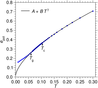
Figure 1 shows the potential energy per particle, $e_{\rm pot}$, as a function of temperature. In this plot, the critical MCT temperature at $T_{c}=0.104$ as well as the glass transition temperature at $T_{g}=0.06$ are indicated. The MCT temperature $T_{c}$ was determined from fits to dynamic quantities such as the mean-square displacement (see below). Below $T_{g}$, the hybrid MD-SMC runs on the time scale of $10^{5}\,\tau_{\rm MD}$ are no longer sufficient to fully equilibrate the system. The data for $T\geq T_{g}$ can be well described by the function (solid line in Fig. 1)

$$f(T)=A+BT^{\gamma}$$ (2)

with $A$, $B$, and $\gamma$ being fit parameters. While the density functional theory of Rosenfeld and Tarazona rosenfeld1998 predicts the exponent $\gamma=0.6$ for simple high-density soft-sphere fluids, we find the exponent $\gamma\approx 0.64$ which is very close to this prediction. Note that Eq. (2) with a value of $\gamma$ around 0.6 also provides a good approximation for other glassforming liquids with a $1/r^{n}$-type interactions at low temperature (for a detailed discussion see Ref. ingebrigtsen2013 ).

Figure 2: a) MSD as a function of time for temperatures $T<T_{g}$ (dashed blue lines), $T_{g}\leq T<T_{c}$ (solid blue lines), and $T>T_{c}$ (red solid lines). b) MSDs at $T=0.11$, $T=0.09$, $T=0.07$, and $T=0.06$. The dashed lines are fits to Eq. (4) and the filled circles mark the location of the life time $\tau_{\rm lt}$ for the different temperatures (see text). The inset is a schematic plot of the MSD that illustrates the definition of $\tau_{\rm lt}$. c) Life time $\tau_{\rm lt}$ as a function of inverse temperature. The solid line is a fit with an Arrhenius law (see text). The MSDs in a) and b) correspond to systems with $N=2048$ particles.

Now we come to the one-particle dynamics of the system and investigate the MSD of a tagged particle, defined by

$$\left\langle\delta r^{2}(t)\right\rangle=\frac{1}{N}\sum_{i=1}^{N}\left\langle|\vec{r}_{i}(t)-\vec{r}_{i}(0)|^{2}\right\rangle$$ (3)

with $\vec{r}_{i}(t)$ the position of particle $i$ at time $t$. The brackets $\langle\dots\rangle$ represent an ensemble as well as a time average over the different samples. Note, however, that for states below $T_{g}$ we have only applied an ensemble average. The MSDs are calculated from microcanonical MD simulation for a system of $N=2048$ particles, using as initial configurations 60 independent samples from the MD-SMC simulations.

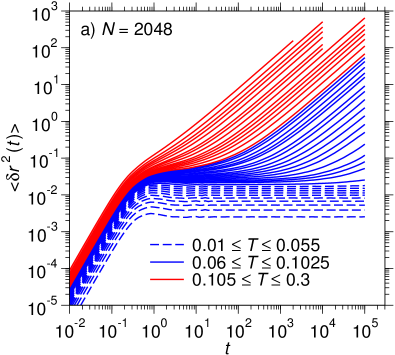
In Fig. 2a, MSDs are plotted double-logarithmically for different temperatures. Here, we have marked the different temperature regimes. The red solid lines correspond to temperatures above $T_{c}$ at $T=0.105$, 0.11, 0.115, 0.12, 0.125, 0.13, 0.14, 0.15, 0.16, 0.18, 0.20, 0.22, 0.25, and 0.3. At the highest temperature, $T=0.3$, the MSD displays a ballistic regime $\propto t^{2}$ at very short times, an emerging shoulder at intermediate times, and a diffusive regime $\propto t$ in the long-time limit. With decreasing temperature, the diffusive regime shifts to longer times and the intermediate time regime evolves into a plateau. The blue solid lines show the MSDs for temperatures $T_{g}<T<T_{c}$ at $T=0.06$, 0.065, 0.0675, 0.07, 0.075, 0.0775, 0.08, 0.0825, 0.085, 0.0875, 0.09, 0.0925, 0.095, 0.0975, 0.10, and 0.1025. Here, the initial configurations are fully equilibrated samples from the MD-SMC simulations. However, the microcanonical MD runs over a time scale of $10^{5}\,\tau_{\rm MD}$ are not long enough to reach a diffusive regime far below $T_{c}$. So at $T=0.06$, we hardly see deviations from the plateau at long times. The MSDs below $T_{g}$ in Fig. 2a (blue dashed lines) correspond to the temperatures $T=0.01$, 0.015, 0.02, 0.025, 0.03, 0.035, 0.04, 0.045, 0.05, and 0.055. Here, the MSDs display a plateau for $1\leq t\leq 10^{5}$, the height of which decreases with decreasing temperature. Note that the small overshoot in the low-temperature MSDs around $t\approx 0.8$ is associated with the microscopic dynamics horbach1996 ; horbach2001 . This feature disappears for larger system sizes (e.g. for our model it cannot be seen anymore for systems with $N=10000$ particles).

The emergence of a shoulder that evolves into a plateau at low temperature manifests the caging of the particles. MCT provides detailed predictions about the behavior of the MSD around the plateau (as well as corresponding predictions for the plateau-like regions in intermediate scattering functions goetze2009 ). One of them describes the initial increase of the MSD from the plateau and is given by goetze2009

$$\phi(t)=\delta r^{2}_{\rm plateau}+ht^{b}+h_{2}t^{2b}\,.$$ (4)

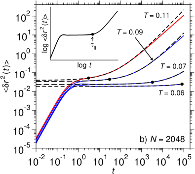
This equation corresponds to a von Schweidler law, extended by a correction term $\propto t^{2b}$. $\delta r^{2}_{\rm plateau}$ quantifies the height of the (emerging) plateau in the MSD, $h$ and $h_{2}$ are temperature-dependent amplitudes, and the exponent $b$ is expected to be universal for a given system (but it may vary for different systems in the range $0<b\leq 1$). Figure 2b shows the MSDs at $T=0.11$, $T=0.09$, $T=0.07$, and $T=0.06$ together with fits to Eq. (4). These fits and also the fits to the MSDs at the other temperatures were performed with the constant exponent value $b=0.59$. Note, however, that the values for $\delta r^{2}_{\rm plateau}$, as obtained from the fit to Eq. (4), are not very sensitive with respect to the choice of the exponent $b$.

Using the fits to Eq. (4), we can now introduce a definition of the life time $\tau_{\rm lt}$ of the transient amorphous solid state for the different temperatures. To this end, we define $\tau_{\rm lt}$ as the time for which $\left\langle\delta r^{2}(\tau_{\rm lt})\right\rangle/\delta r^{2}_{\rm plateau}=1.3$ (see the inset of Fig. 2b for an illustration of this definition). The locations of $\tau_{\rm lt}$ for the MSDs in Fig. 2b are marked as filled circles.

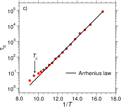
Figure 2c shows the logarithm of the time scale $\tau_{\rm lt}$ as a function of inverse temperature. For $T\lesssim 0.09$, the data can be well fitted by an Arrhenius law $f(T)=\tau_{0}\,\exp\left(E_{\rm A}/T\right)$, which is represented by the bold solid line in the figure. The values of the fit parameters are $\tau_{0}=3.3\times 10^{-6}$ and $E_{\rm A}=1.43641$. Here, the energy $E_{\rm A}$ can be interpreted as an activation energy. The application of the Arrhenius law and thus the interpretation of a kinetic process as an activated one are only sensible if the ratio of the activation energy to the thermal energy, $E_{\rm A}/T$, is much larger than unity riskenbook . In our case, this ratio varies between about 16 at $T=0.09$ and about 24 at $T=0.06$ which is consistent with the condition $E_{\rm A}/T\gg 1$. At temperatures $T\gtrsim T_{c}$, we observe significant deviations from the Arrhenius behavior and $\tau_{\rm lt}$ is close to the microscopic time scale $\tau_{\rm MD}$. From the temperature dependence of $\tau_{\rm lt}$ we can conclude that around $T_{c}$ there is a gradual crossover towards an activated dynamics with decreasing temperature.

Figure 3: Localization length divided by the mean nearest-neighbor distance, $\xi/\bar{d}$, as a function of temperature. The dashed red line marks the critical value of the reduced localization length, $\xi_{c}/\bar{d}\approx 0.077$.

In the framework of the Gaussian approximation hansenbook ; thorneywork2016 ; fuchs1998 , one can relate $\delta r^{2}_{\rm plateau}$ to a localization length $\xi$ as

$$\xi^{2}=\frac{1}{6}\delta r^{2}_{\rm plateau}\,.$$ (5)

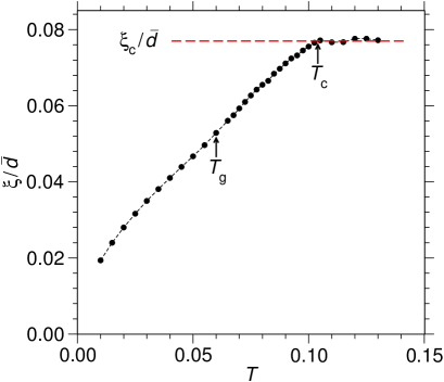
Figure 3 shows the temperature dependence of $\xi$, scaled with the average nearest-neighbor distance $\bar{d}\approx 1.07$ (we have estimated $\bar{d}$ from the location of the first peak of the radial distribution function at $T=0.06$). At $T=0.01$, i.e. far below $T_{g}$, the reduced localization length is $\xi/\bar{d}\approx 0.02$. It increases with increasing temperature. At $T_{g}$, $\xi/\bar{d}$ slightly changes slope and then increases roughly linearly up to $T_{c}$ where it reaches the constant $\xi_{c}/\bar{d}\approx 0.077$. The critical value, $\xi_{c}$, of the localization length marks the stability limit of the amorphous solid, i.e. for $T>T_{c}$ the system is in a liquid state. In analogy to crystalline solids, the critical value $\xi_{c}/\bar{d}$ can be interpreted as a Lindemann criterion for the stability of an amorphous solid goetze2009 . Note that Fuchs et al. fuchs1998 have obtained $\xi_{c}/\bar{d}\approx 0.0746$ in a calculation for a hard sphere system in the framework of MCT, thus a value that is very close to our finding.

The behavior of both $\tau_{\rm lt}$ and $\xi$ indicate a gradual change of the dynamics around $T_{c}$. Below $T_{c}$, the localization of particles in their cages, as quantified by $\xi_{c}/\bar{d}$, is below the stability limit, given by $\xi_{c}/\bar{d}\approx 0.077$. As a consequence, there is the emergence of transient amorphous solid state for $T<T_{c}$, the life time $\tau_{\rm lt}$ of which follows an Arrhenius law with an activation energy of about 1.44. The gradual change from liquid-like to solid-like dynamics is also associated with a qualitative change of the system’s response to an external shear. As we shall see in the next section, brittle yielding and the formation of shear bands can be observed in the supercooled liquid below $T_{c}$. These features are typical for the response of low-temperature glasses to a mechanical load. In the following, we shall analyze the conditions for the occurrence of brittle yielding and shear banding in deeply supercooled liquids. An important parameter in this context is the time scale $\tau_{\rm lt}$. For example, for $T=0.06$, the life time $\tau_{\rm lt}$ is of the order of $10^{5}$ (Fig. 2c). Therefore, for $\dot{\gamma}\gtrsim 10^{-5}$, the product $\dot{\gamma}\tau_{\rm lt}$ is lower equal unity and one may expect the shear response of an amorphous solid.

IV Supercooled liquids under shear

Now we analyze the results for equilibrated supercooled liquids under shear. Our focus is on the temperature range $0.06\leq T\leq 0.15$ to study the response to the external shear from liquid-like states slightly above $T_{c}$ to the solid states far below $T_{c}$. As we have seen in the previous section, the latter states can be characterized via the localization length $\xi$ being significantly lower than the critical value $\xi_{c}$.

Figure 4: Stress-strain relation for the temperature $T=0.06$ and the shear rate $\dot{\gamma}=10^{-3}$. Indicated are the maximum $\sigma_{\rm max}$, the steady-state stress $\sigma_{\rm ss}$, and the definition of the stress drop $\Delta\sigma$.

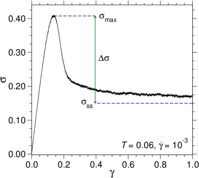
A typical stress-strain relation, indicating a non-Newtonian response of the supercooled liquid, is shown in Fig. 4 for the temperature $T=0.06$ and the shear rate $\dot{\gamma}=10^{-3}$. While the strain is given by $\gamma=\dot{\gamma}t$, the stress $\sigma$ was computed from the virial equation, as described in Ref. golkia2020 . Different regimes can be identified in the figure. First the stress increases almost linearly up to a maximum value $\sigma_{\rm max}$ which is reached at a strain $\gamma\approx 0.135$ in this case. The maximum in the stress marks the transition from an elastic deformation of the “solid” to the onset of plastic flow. During the plastic deformation, the stress drops from $\sigma_{\rm max}$ towards the steady-state stress $\sigma_{\rm ss}$ which can be quantified by $\Delta\sigma=\sigma_{\rm max}-\sigma_{\rm ss}$. In the steady state, the system can be described by a flowing homogeneous liquid. Heterogeneous flow patterns are observed between the onset of plastic flow and the steady state. The morphology of these flow patterns, especially with respect to the dependence on temperature and shear rate, shall be elucidated in the following.

Figure 5: Flow curves for the temperatures $T=0.06$, 0.09, 0.11, and 0.15. The solid line is a fit with a Herschel-Bulkley law to the data for $T=0.06$ (see text). The dashed line indicates a linear behavior, $\sigma_{\rm ss}\propto\dot{\gamma}$.

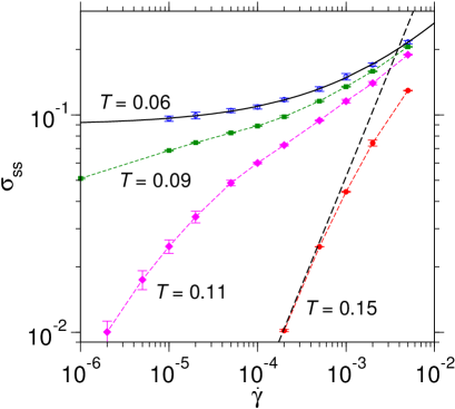
In Fig. 5, the steady-state stress $\sigma_{\rm ss}$ as a function of the shear rate $\dot{\gamma}$ (i.e. the flow curve) is plotted double-logarithmically for different temperatures above and below $T_{c}$. For sufficiently low shear rates, one expects that the system behaves like a Newtonian fluid with a linear increase of the stress as a function of the shear rate, $\sigma_{\rm ss}=\eta\dot{\gamma}$ (with $\eta$ the shear viscosity). At $T=0.15$, we can still identify a Newtonian regime (dashed line), followed by sublinear shear-thinning regime for $\dot{\gamma}>5\times 10^{-4}$. At $T=0.11$, the Newtonian regime is not anymore in the window of considered shear rates $\dot{\gamma}\geq 10^{-6}$. Here, we observe an emerging plateau around $\dot{\gamma}=10^{-4}$ that becomes more pronounced at $T=0.09$, and eventually, at $T=0.06$, the data can be well fitted by a Herschel-Bulkley law herschel1926 (solid line), $\sigma_{\rm ss}=\sigma_{\rm yield}+A\dot{\gamma}^{\alpha}$ with the yield stress $\sigma_{\rm yield}=0.0900265$, the amplitude $A=1.57446$, and the exponent $\alpha=0.477008$. Note that at $T=0.07$ the flow curve is very similar to that at $T=0.06$. So at the lowest considered temperatures where we are able to obtain a fully equilibrated state, our system can be seen as a yield stress material in equilibrium (although we also expect at these temperatures the occurrence of a Newtonian regime at extremely low shear rates).

Figure 6: Reduced stress $\sigma^{\star}$ as a function of $\gamma-\gamma_{\rm max}$ at the different temperatures $T=0.06$, 0.07, and 0.09 for the shear rates a) $\dot{\gamma}=10^{-3}$, b) $\dot{\gamma}=10^{-4}$, and c) $\dot{\gamma}=10^{-5}$. The data corresponds to systems with $N=10000$ particles. In c), the dotted lines correspond to data for $N=12000$ and $N=96000$, as adapted from Ref. ozawa2018 . The dashed and the dotted line in a) are fits with with a compressed exponential and a logarithm, respectively (see text).

Having characterized the steady-state behavior of our system under shear, we now investigate the relaxation of the stress from the onset of plastic flow (marked by the maximum stress $\sigma_{\rm max}$ at a given temperature) to the steady-state stress. To this end, we define the reduced stress

$$\sigma^{\star}=\frac{\sigma-\sigma_{\rm ss}}{\sigma_{\rm max}-\sigma_{\rm ss}}$$ (6)

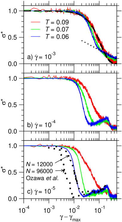
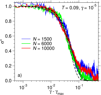
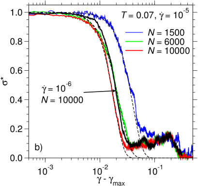
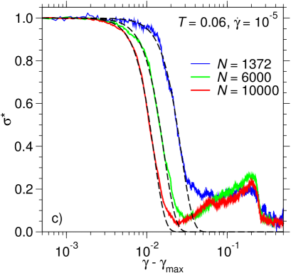
which is displayed in Fig. 6 for three shear rates and three temperatures below $T_{c}$ as a function of $\gamma-\gamma_{\rm max}$ (with $\gamma_{\rm max}$ the strain corresponding to $\sigma_{\rm max}$). At $\dot{\gamma}=10^{-3}$ (Fig. 6a), the decay of $\sigma^{\star}$ for $T=0.09$ can be described by the compressed exponential $\exp[-((\gamma-\gamma_{\rm max})/\delta\gamma^{\star})^{a_{\rm ce}}]$ with $\delta\gamma^{\star}=0.115946$ and $a_{\rm ce}=1.33297$. Also for the two lower temperatures $T=0.06$ and 0.07, the reduced stress decays on a strain scale $\delta\gamma^{\star}\approx 0.1$, but the functional form of its decay changes around $\gamma-\gamma_{\rm max}\approx 0.08$ in that the compressed-exponential-like decay is followed by a logarithmic one $\propto\ln[(\gamma-\gamma_{\rm max})/1.07353]$ (dotted line in Fig. 6a, fitted to the “tail” of the $T=0.06$ curve). The difference in the decay of $\sigma^{\star}$ with respect to temperature becomes more pronounced at the lower shear rates $10^{-4}$ (Fig. 6b) and $10^{-5}$ (Fig. 6c). While at $T=0.09$, the reduced stress still decays essentially with a compressed exponential on the strain scale $\delta\gamma^{\star}\approx 0.1$, at the two lower temperatures the initial decay is significantly faster and $\sigma^{\star}$ exhibits a local maximum around $\gamma-\gamma_{\rm max}\approx 0.2$. The strain scale of the initial decay decreases with decreasing temperature and shear rate. At $T=0.06$ and $\dot{\gamma}=10^{-5}$, the reduced stress $\sigma^{\star}$ decays on the strain scale $\delta\gamma^{\star}\approx 0.01$.

Also included in Fig. 6c are data for $N=12000$ and $N=96000$, as adapted from the simulation study of Ozawa et al. ozawa2018 using an aqs protocol. It is remarkable that the reduced stress for $N=12000$ from Ozawa et al. agrees well with our data for a comparable system of $N=10000$ particles, although we consider a system at a finite temperature as well as a finite strain rate and, moreover, our system is in an equilibrated supercooled liquid state (note, however, that $\sigma_{\rm max}$ is significantly larger in the athermal case).

Figure 7: Reduced stress $\sigma^{\star}$ as a function of $\gamma-\gamma_{\rm max}$ at the shear rate $\dot{\gamma}=10^{-5}$ and temperatures a) $T=0.09$, b) $T=0.07$, and c) $T=0.06$ for different system sizes, as indicated. The dashed lines are fits with compressed exponentials (see text). Also included in b) is the reduced stress for $\dot{\gamma}=10^{-6}$ and $N=10000$.

It is tempting to interpret the rapid drop of the stress as a first-order phase transition, as proposed by Ozawa et al. ozawa2018 . The interpretation of the stress drop as a phase transition would be appropriate in the limit of zero shear rate, $\dot{\gamma}\to 0$. So we have to take this limit in some sensible manner, keeping in mind that the expected true behavior of the system in the zero shear-rate limit is that of a Newtonian fluid for which $\sigma_{\rm ss}\propto\dot{\gamma}$ and the absence of any stress drop in the stress-strain relation. However, the fluid curves for $T\leq 0.07$ suggest that the systems can be considered as a yield stress fluid also at very low shear rates and one obtains $\sigma_{\rm yield}$ by extrapolation via the Herschel-Bulkley law. Below, we perform a similar extrapolation to obtain the initial strain scale $\delta\gamma^{\star}$ with which the stress decays from $\sigma_{\rm max}$ to $\sigma_{\rm ss}$ in the limit $\dot{\gamma}\to 0$.

The existence of a first-order transition in the thermodynamic limit implies that it is rounded for finite systems and it becomes sharper with increasing system size. Figure 7 shows the decay of the reduced stress $\sigma^{\star}$ for different system sizes at the temperatures $T=0.09$, $T=0.07$, and $T=0.06$ in panels a), b), and c), respectively. For all three temperatures, the shear rate is $\dot{\gamma}=10^{-5}$. While for $T=0.09$ there is almost no dependence of $\sigma^{\star}$ on system size, for the two lower temperatures the decay of $\sigma^{\star}$ becomes significantly sharper with increasing system size. For $T=0.07$ (Fig. 7b), we have also included the reduced stress for the lower shear rate $\dot{\gamma}=10^{-6}$ and $N=10000$ which exhibits a less rapid decay than the corresponding result for $\dot{\gamma}=10^{-5}$. This can be explained in terms of the life time $\tau_{\rm lt}$ in relation to the shear rate $\dot{\gamma}$. Above we have estimated $\tau_{\rm lt}\approx 3300$ for $T=0.07$ (cf. Fig. 2c) and thus the time scale $\dot{\gamma}^{-1}$ is much larger than $\tau_{\rm lt}$ for both shear rates $10^{-5}$ and $10^{-6}$. The yielding of the system interferes with structural relaxation processes in this case and this certainly in a more pronounced manner for $\dot{\gamma}=10^{-6}$ than for $\dot{\gamma}=10^{-5}$. Therefore, the reduced stress decays faster for the higher shear rate of $\dot{\gamma}=10^{-5}$.

The dashed lines in Fig. 7 are fits with compressed exponentials. In these fits, the exponent $a_{\rm ce}$ is around 3.0 and the strain scale changes from $\delta\gamma^{\star}\approx 0.027$ for $N=1000$ to $\delta\gamma^{\star}\approx 0.012$ for $N=10000$. While the initial decay of $\sigma^{\star}$ strongly depends on $N$, the second feature in $\sigma^{\star}$, the appearance of a local maximum at $\gamma-\gamma_{\rm max}\approx 0.2$, does not show significant finite-size effects.

Figure 8: Strain scale $\delta\tilde{\gamma}^{\star}$ as a function of shear rate $\dot{\gamma}$ at the temperatures $T=0.07$ [a)] and $T=0.06$ [b)] for different system sizes. In b), the solid lines are fits with the function $g(\dot{\gamma})=\delta\tilde{\gamma}^{\star}_{0}+A_{\gamma}\dot{\gamma}^{c_{\gamma}}$ (for details see text). The inset shows $\delta\tilde{\gamma}^{\star}_{0}$ as a function of $N^{-1}$.

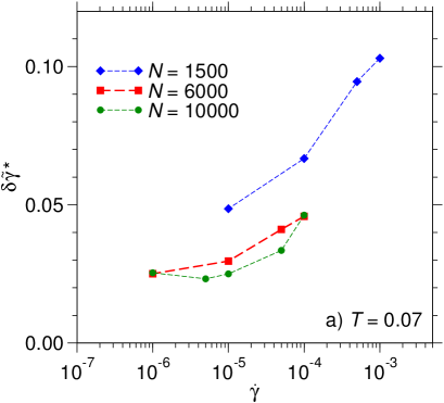
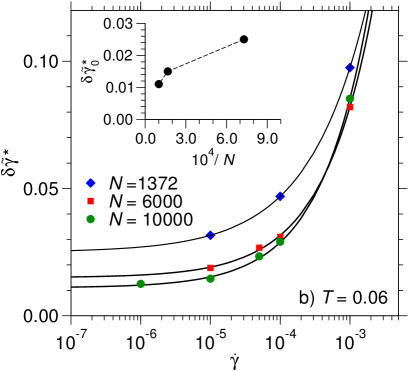
In the following, we do not use the strain scale, as directly obtained from the fits to the compressed exponentials. In lieu thereof, we use the value where the reduced stress, as described by the compressed exponential, has decayed to 0.2. We denote this quantity by $\delta\tilde{\gamma}^{\star}$. Figure 8 displays the shear-rate dependence of $\delta\tilde{\gamma}^{\star}$ for $T=0.07$ in a) and $T=0.06$ in b) and different system sizes. In the case of $T=0.07$, the transition becomes significantly sharper for all shear rates when changing the particle number from $N=1500$ to $N=6000$. However, only small changes are observed when going from $N=6000$ to $N=10000$ (at $\dot{\gamma}=10^{-6}$, the values for $\delta\tilde{\gamma}^{\star}$ are essentially equal for the two system sizes). This is due to the fact that the life time $\tau_{\rm lt}$ is smaller than the time scale $\dot{\gamma}^{-1}$ for $\dot{\gamma}\leq 10^{-4}$ and thus the yielding transition interferes with relaxation processes in the liquid.

In Fig. 8b for $T=0.06$, the solid lines correspond to the fit function $g(\dot{\gamma})=\delta\tilde{\gamma}^{\star}_{0}+A_{\gamma}\dot{\gamma}^{c_{\gamma}}$, with $\delta\tilde{\gamma}^{\star}_{0}$ the estimate of $\delta\tilde{\gamma}^{\star}$ at zero shear rate, $A_{\gamma}$ an amplitude, and $c_{\gamma}$ an exponent that has value of about $0.62$ in the fits of Fig. 8b. Thus, the zero shear-rate values of the strain scale can be well estimated via a “Herschel-Bulkley-like” law. The inset of Fig. 8b shows $\delta\tilde{\gamma}^{\star}_{0}$ as a function of $N^{-1}$. In the considered range of system sizes, we observe a weak dependence of $\delta\tilde{\gamma}^{\star}_{0}$ on system size. The data suggests that there might be a regime $\propto 1/N$ for large $N$, similar to what one expects for a first-order phase transition. However, our data is not conclusive to support this interpretation.

But what happens at this yielding transition? And what is the meaning of the second feature in $\sigma^{\star}$, i.e. the increase of $\sigma^{\star}$ up to a maximum around $\gamma-\gamma_{\rm max}=0.2$? Below we show that both features are connected to the formation of shear bands. The rapid initial decay of $\sigma^{\star}$ is a manifestation of brittle yielding.

Figure 9: Stress-strain relations for a) horizontal shear bands and b) vertical shear bands at the temperature $T=0.06$ and the shear rate $\dot{\gamma}=10^{-5}$ in the main figures and for different shear rates in the insets. The grey lines in the main plots are the stress-strain relations for the individual runs and the black lines correspond to the average over these runs.

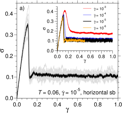
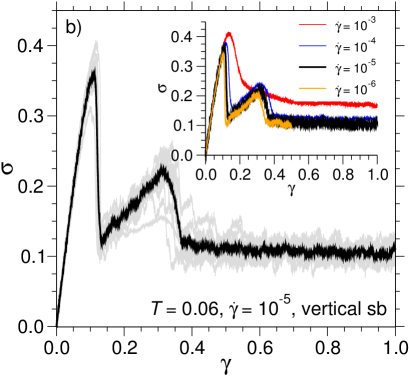
To analyze the behavior of the system around yielding, we now consider individual runs at the temperature $T=0.06$ and the shear rate $\dot{\gamma}=10^{-5}$. Among the 30 independent runs for the systems with $N=10000$ particles, we find two types of stress-strain relations. In both cases, we observe an initial sharp drop, indicating brittle yielding. However, while we see in the first type only the initial stress drop (Fig. 9a), in the second one there is the additional increase after the first drop up to $\gamma\approx 0.32$, followed by a second drop of the stress (Fig. 9b). The first type of stress-strain relation corresponds to the formation of a horizontal shear band, i.e. the occurrence of a thin melted layer with an orientation parallel to the flow direction. The second type of stress-strain relation corresponds to the initial formation of a vertical shear band where the melted thin layer is oriented perpendicular to the flow direction. Note that among the 30 runs, we have observed horizontal and vertical shear bands in 18 and in 12 cases, respectively. In Fig. 9, the grey lines correspond to the individual runs and black ones to the average over these runs in each case. The insets of Fig. 9 show the averaged stress-strain relations for different shear rates. For $\dot{\gamma}\leq 10^{-4}$, a qualitatively similar behavior is seen with essentially the initial stress drop getting slightly sharper with decreasing shear rate (cf. Fig. 8). At $\dot{\gamma}=10^{-3}$, however, the yielding transition is washed out and, instead of the second maximum in the stress-strain relation for the vertical shear bands, there is a logarithmic decay around $\dot{\gamma}=0.3$ (cf. Fig. 6a).

Figure 10: Potential energy per particle as a function of strain for a) horizontal shear bands and b) vertical shear bands at the temperature $T=0.06$ and the shear rate $\dot{\gamma}=10^{-5}$ in the main figures and for different shear rates in the insets. The grey lines in the main plots are the stress-strain relations for the individual runs and the black lines correspond to the average over these runs. The horizontal dashed lines in both panels mark the average steady-state value, $\bar{e}_{\rm pot}=0.305$.

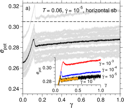
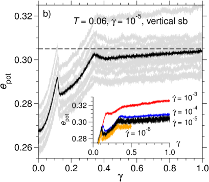
The brittle yielding is also reflected in the behavior of the potential energy per particle, $e_{\rm pot}$, as a function of the strain $\gamma$. In the case of the horizontal shear bands at $T=0.06$ and $\dot{\gamma}=10^{-5}$ (Fig. 10a), there is first a drop of $e_{\rm pot}$ at the yield point, followed by a slow increase towards the steady-state value which is at about $\bar{e}_{\rm pot}=0.305$ (horizontal dashed line). As can be inferred from the figure, there is a large scatter in the values of $e_{\rm pot}$ from sample to sample. This is due to the polydispersity of the samples. However, the shape of the curves for the different samples is very similar and they are essentially shifted with respect to each other. This is also true for the behavior of $e_{\rm pot}$ vs. $\gamma$ for the case of the vertical shear bands (Fig. 10b). Here, after the first drop of the energy, it increases to a value which is close to the steady-state value, then, around $\gamma\approx 0.3$ (corresponding to the local maximum in the stress-strain relation), it slightly decreases before it increases towards the steady-state value. For the case of the vertical shear bands, the system reaches the steady state much faster than in the case of the horizontal shear bands. The behavior of $e_{\rm pot}(\gamma)$ for the different shear rates (see insets of Fig. 10) is similar to that of the corresponding stress-strain relations.

Figure 11: Mobility maps at $T=0.06$ and $\dot{\gamma}=10^{-5}$ for a sample with the formation of a horizontal shear band for a) $\gamma=0.1024$, b) $\gamma=0.1472$, and c) $\gamma=0.495$ and a sample with the formation of a vertical shear band for the same values of $\gamma$, d) - f).

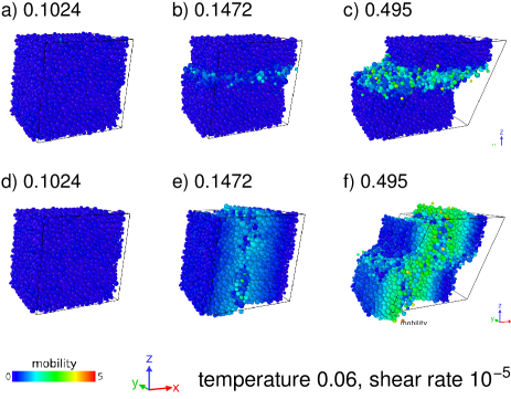
To visualize the shear bands, mobility color maps shriva2016_1 are computed. To this end, we determine, for each particle $i$, the non-averaged MSDs $\delta y_{i}^{2}(t)$ and $\delta z_{i}^{2}(t)$ in the neutral $y$ direction and the shear-gradient $z$ direction, respectively. From this, we obtain the “mobility displacement” $\Delta_{i}(t)=\sqrt{\delta y_{i}^{2}(t)+\delta z_{i}^{2}}$ and we assign a color to the magnitude of $\Delta_{i}$. The time origin for the calculation of $\Delta_{i}$, $t=0$, corresponds to the time where the external shear is switched on. For the snapshots in Fig. 11 at different values of the strain, we have selected a sample with a horizontal shear band [a)-c)] and one with a vertical shear band [d)-f)], both samples are at $T=0.06$ and $\dot{\gamma}=10^{-5}$. At $\gamma=0.1024$, i.e. just before the onset of plastic flow, the system is in a homogeneously deformed state and therefore the mobility of the particles is close to zero, as represented by the blue color. At the strain $\gamma=0.1472$ a horizontal shear band has formed in the first sample (Fig. 11b) and a vertical one in the second sample (Fig. 11e). In both cases, the fluidized regions along the band are represented by particles, colored in green. The horizontal shear band exhibits a slow growth as a function of strain, as reflected, e.g., in a slow increase of the potential energy of the system (cf. Fig. 10a). At $\gamma=0.495$, the thickness of the horizontal shear band corresponds to about 5-6 $\sigma$, i.e. a few liquefied layers (Fig. 11c). The behavior is different in the case of the vertical shear band. Here, the thickness of the vertical band first increases which is accompanied by an increase of the stress with increasing strain (cf. Fig. 9b). The stress drop at $\gamma\approx 0.3$ is associated with the formation of an additional horizontal shear band which grows with increasing strain (cf. Fig. 11f).

V Summary and conclusions

In summary, we have investigated the yielding behavior of a glassforming soft-sphere model under shear. Using molecular dynamics (MD) simulation in combination with the swap Monte Carlo (SMC) technique, fully equilibrated supercooled liquid samples around and far below the critical mode coupling temperature $T_{c}$ were obtained.

First, these samples served as starting configurations for simulations in the microcanonical ensemble to study how the dynamics of the supercooled liquid changes when decreasing the temperature from above to far below $T_{c}$. In qualitative agreement with mode coupling theory (MCT), we have seen that the reduced localization length $\xi/\bar{d}$, as extracted from the mean squared displacement, shows a kink at $T_{c}$, changing from $\xi_{c}/\bar{d}=0.077$ for $T>T_{c}$ to a roughly linearly decreasing function for decreasing temperature below $T_{c}$. Here, the critical value $\xi_{c}/\bar{d}$ marks the stability limit of the amorphous solid. In fact, the decrease of $\xi$ with decreasing temperature is accompanied by an exponential increase of a time scale $\tau_{\rm lt}$ that measures the life time of the amorphous solid state. The Arrhenius law that we find for the temperature dependence of $\tau_{\rm lt}$ is consistent with the interpretation of an activated dynamics for structural relaxation processes below $T_{c}$.

The gradual change of structural relaxation from a liquid-like to a solid-like dynamics around $T_{c}$ is associated with a change of the system’s response to a mechanical load, in particular with respect to the yielding of the system. In this work, we have studied sheared supercooled liquids in a planar Couette flow geometry, applying a constant shear rate $\dot{\gamma}$. We have shown that the emergence of a transient amorphous solid state implies the possibility of brittle yielding which is characterized a sharp stress drop in the stress-strain relation. This means that around a strain of the order of 0.1, the stress shows a sudden decrease on a strain scale $\delta\tilde{\gamma}^{\star}$ much less than 0.1 (this value is found for the stress decay at yielding for temperatures above and around $T_{c}$). For example, at a temperature $T=0.06$ and a shear rate $\dot{\gamma}=10^{-5}$, we find $\delta\tilde{\gamma}^{\star}=0.014$. While at low temperatures, $T\ll T_{c}$, $\delta\tilde{\gamma}^{\star}$ significantly decreases with increasing system size, our data is not conclusive with respect to the question whether brittle yielding can be interpreted in terms of an underlying kinetic first-order transition in the limit $\dot{\gamma}\to 0$. Anyway, at finite temperature, such an interpretation has to be taken with a grain of salt. On the one hand, the signatures of a first-order transition can be only seen on the time scale $\tau_{\rm lt}$ and thus for shear rates $\dot{\gamma}$ with $\dot{\gamma}\tau_{\rm lt}\gtrsim 1$ (note that for $\dot{\gamma}\tau_{\rm lt}\gg 1$, one expects Newtonian behavior). On the other hand, at a given temperature $T<T_{c}$, the shear rate has to be small enough that the steady-state stress is close to the apparent yield stress, as obtained from the extrapolation to $\dot{\gamma}\to 0$ in terms of a Herschel-Bulkley law. Thus, the time scale $\tau_{\rm lt}$ has to be very large in order to see the signatures of a first-order transition and this is the case for temperatures far below $T_{c}$. As similar interplay of time scales has been recently found by Shrivastav and Kahl shrivastav2021 , studying the yielding in a cluster crystal.

Brittle yielding is associated with horizontal or vertical shear bands. Both types of shear bands are equally efficient to release the stress at the yield strain. The mechanism for the formation of such shear bands at finite temperatures and shear rates is still not well understood, but for the transient amorphous solid states under equilibrium conditions, as studied in this work, techniques and theoretical frameworks can be adapted that have been previously mainly used for athermal systems, such as an analysis of soft modes determined from the dynamical matrix jaiswal2016 ; procaccia2017 ; parisi2017 . Another promising framework to investigate the yielding transition and shear banding in amorphous solids is the analysis in terms of non-affine displacements falk1998 ; lemaitre2006 ; ganguly2013 ; ganguly2015 ; baggioli2021 , as recently applied to elucidate plasticity and yielding in crystalline solids ganguly2017 ; nath2018 ; reddy2020 . Work in this direction is in progress.