Effect of quantum jumps on non-Hermitian system

Abstract

One among the possible realizations of non-Hermitian systems is based on open quantum systems by omitting quantum jumping terms in the master equation. This is a good approximation at short times where the effects of quantum jumps can be ignored. However, the jumps can affect the long time dynamics of the system, motivating us to take the jumps into account in these studies. In this paper, by treating the quantum jumps as perturbations, we examine the effect of the quantum jumps on the non-Hermitian system. For this purpose, we first derive an effective Hamiltonian to describe the dynamics of the open quantum system based on the master equation, then expand the eigenstates and eigenenergies up to the first and second order in the quantum jumps. Finally, we apply our theory to a dissipative two-level system and dissipative fermionic superfluids. The effect of quantum jump on the dynamics and the nonequilibrium phase transition is demonstrated and discussed.

I INTRODUCTION

In recent years, non-Hermitian (NH) systems bender2007making have attracted much attention ashida2020nonhermitian from both sides of theoretical and experimental studies. Without the restriction of Hermiticity, non-Hermitian Hamiltonians have been applied to re-examine well-known quantum systems ranging from single-particle to many-body systems lee2014heralded ; yoshida2019nonhermitian ; xu2020topological ; liu2020nonhermitian ; yaoEdgeStatesTopological2018 . Interesting features and novel observations are found, including phase transitions lourenco2018kondo , exception points (EPs) berry2004physics ; hassan2017dynamically ; chen2017exceptional ; lai2019observation , quantum skin effect hagaLiouvillianSkinEffect2021 ; okuma2020topological ; lee2020manybody , non-Bloch bulk-boundary correspondence yaoEdgeStatesTopological2018 ; wang2020defective , unidirectional zero reflection shen2018synthetic ; yan2020unidirectional and so on.

Non-Hermitian systems differ from their Hermitian counterparts in many aspects, such as the non-conservation of probability, complex-valued eigen-energies and biorthonormal eigenstates brody2014biorthogonal . In order to obtain an effective NH Hamiltonian, many works suggest using open quantum system lee2014heralded ; yamamoto2019theory ; liu2020nonhermitian ; xu2020topological ; yoshida2019nonhermitian ; yang2021exceptional by neglecting quantum jumps, adding reciprocal terms into Hermitian systems yaoEdgeStatesTopological2018 ; lee2020manybody ; gong2018topologicala , or using parametric-amplifier type interactions wang2019nonhermitian . Among them, the most popular scheme is the open system approach, which neglects the quantum jumps in the Lindblad master equation and is valid at the short time limit defined by the loss rate $1/\gamma$ yamamoto2019theory ; yoshida2019nonhermitian ; xu2020topological ; durrliebliniger . It is worth addressing that the validity of ignoring the jumps also depends on initial states of the dynamics.

The quantum jumps are associated with the terms in the quantum master equation that act on both left and right side of the density matrix. From the viewpoint of measurement, the environment can be treated as a device, which continuously measures the system and the quantum jumps cause an abrupt change in the state of the system. According to the quantum trajectory theory, the quantum jumps are the terms responsible for the abrupt stochastic change of the wave function. The quantum jumps can also result in different properties of the exceptional points (EPs). In fact, for Lindbladians with and without quantum jumps minganti2019quantum ; chen2021quantum , the EPs can be remarkably different. Connections between the two types of EPs are established by introducing a hybrid-Liouvillian superoperator, where “hybrid” denotes Liouvillian with different strength of jumping terms, which is capable to describe the passage from a non-Hermitian Hamiltonian to a true Liouvillian including quantum jumps minganti2020hybridliouvillian .

Generally speaking, an analytical solution to the master equation is difficult to obtain due to the huge size of the Hilbert space. Several stochastic approaches, for instance, Monte-Carlo molmer1993monte ; dalibard1992wavefunction and quantum-trajectory daley2014quantum are put forward. These approaches apply randomness and statistical laws to simulate the occurrence of quantum jumps, which reduce the complexity from $H_{N}^{2}$ to $H_{N}$ with $H_{N}$ being the size of Hilbert space of the Hamiltonian. However, their numerical simulations are time-consuming and lack of analytical results. To this extent, the non-Hermitian Hamiltonian is a convenient approach to describe open systems. However, dropping the quantum jump terms might lead to a wrong result. Therefore, the examination on the validity of neglecting the quantum jump terms is an urgent task.

In this paper, by using the effective Hamiltonian approach yi2001effective , we propose a method to approximately solve the master equation. The effective Hamiltonian approach can transform the Lindblad master equation into a Schrödinger-like equation with an effective Hamiltonian, which describes the dynamics of a composite system consisting of the system and an auxiliary system. Thus the dynamics governed by the master equation is transformed into an evolution of a pure state governed by the effective Hamiltonian, and the pure state can be mapped back to the density matrix of the system. Here we develop the mapping rule with a biorthonormal basis. By combining the effective Hamitonian approach with NH-perturbation theory sternheim1972nonhermitian ; kato2013perturbation , we formally derive a higher-order approximate solution to the master equation, and illustrate our theory with examples.

This paper is organized as follows. In Sec. II, we introduce the effective NH Hamiltonian approach and combine it with the perturbation theory to derive a solution for the density operator. We first assume that the quantum jump terms in the master equation are negligible, then treat these terms as perturbations. In Sec. III and Sec. IV we apply our method to two-level system with decoherence and a dissipative BCS (Bardeen-Cooper-Schrieffer) system bardeen1957microscopic . We calculate the approximate density operator, energy and the fidelity of initial state by the present theory. The results are discussed and the effect of quantum jumps on the BCS state is analyzed. Finally, we conclude in Sec. V .

II formalism

The Markov master equation is one of the most fundamental descriptions for open systems in quantum theory gardiner2004quantum , which was derived with the weak coupling assumption and the Markov approximation. The master equation is valid in many circumstances, and the solution to the equation obey the basic rules of quantum mechanics such as trace preserving, complete positivity and Hermiticity. This is the reason why a wide range of applications have been developed in various fields including quantum state preparation kraus2008preparation , excitation transfer in light-harvesting systems, quantum measurement walls1985analysis and quantum computation verstraete2009quantum . Due to the complexity of the master equation, many methods have been introduced to approximately solve the equation. For examples, in Ref. kim1996perturbative the authors developed a short-time perturbative expansion method, and Ref. yi2000perturbative presented a perturbation theory by treating the small-loss as the perturbations. Ref. li2015perturbative , decomposes the Liouvillian supperoperator into two parts, treating the part of dissipators as the dominant contribution to the system, while the other parts of the dissipators were treated as perturbations. Based on this, Ref. li2016resummation considered a practical model of damping Jaynes-Cumming lattices, in which the interaction between the resonator mode and the qubit was viewed as a perturbation. Ref. albert2018lindbladians introduced a perturbation theory for a time-dependent Lindbladian master equation with the help of Dyson expansions and linear response theory.

In the following, we will develop a new approach to solve the master equation based on the perturbation theory for non-Hermitian systems, the difference is that the jumping terms in the master equation are treated as the perturbation terms. Let us start with the master equation in the Lindblad form breuer2002theory ; gardiner2004quantum

$$\dot{\rho}\!=\!-i\left[H_{0},\rho\right]\!+\!\sum_{m}\!\frac{\kappa_{m}}{2}\!(2F_{m}\rho F_{m}^{\dagger}\!-\!F_{m}^{\dagger}F_{m}\rho\!-\!\rho F_{m}^{\dagger}F_{m}),$$ (1)

where $H_{0}$ is the free Hamiltonian of the system, $\kappa_{m}$ is the decay rate for the $m$-th decay channel, and $F_{m}$ stands for the eigenoperator of the system, usually named as Lindblad operators. The reduced density matrix $\rho$ remains completely positive and trace preserving lindblad1976generators . However, these break down when the jumping terms are neglected and an effective non-Hermitian Hamiltonian $H=H_{0}-i/2\sum_{m}\kappa_{m}F^{\dagger}_{m}F_{m}$ is persisted to describe the system. Suppose $H$ is diagonalizable and the eigenvectors satisfy

$$H|r_{n}\rangle=E_{n}|r_{n}\rangle,H^{\dagger}|l_{n}\rangle=E_{n}^{*}|l_{n}\rangle,$$ (2)

where $|r_{n}\rangle$ and $|l_{n}\rangle$ are the right and left eigenvectors of $H$. In the following discussion, we will follow the biorthonormal relation $\langle l_{m}|r_{n}\rangle=\delta_{mn}$, and the completeness relation brody2014biorthogonal

$$\sum_{n}|r_{n}\rangle\langle l_{n}|=\sum_{n}|l_{n}\rangle\langle r_{n}|=I.$$ (3)

Since the biorthonormal eigenvectors are also complete brody2014biorthogonal , we can use them to expand the density matrix. Following Ref. yi2001effective , we can obtain an effective Hamiltonian as long as the mapping between the composite system and the density operator is specified. Here we generalize this theory taking different set of eigenstates as the basis. The details of the generalization can be found in Appendix A. We should address that once the relation is established, the effective Hamiltonian is unique

$$\widetilde{H}=H-H^{A*}+i\sum_{m}\kappa_{m}F_{m}F^{A*}_{m},$$ (4)

here the superscript $A$ denotes the auxiliary system, whose matrix representation satisfies

$$\langle r_{m}|O^{\dagger}|l_{n}\rangle=(^{A}\langle L_{n}|O^{A}|R_{m}\rangle^{A})^{*}.$$ (5)

Under the mapping rules, the density operator matrix element is now defined as $\rho_{mn}=\langle l_{m}|\rho|l_{n}\rangle$ and the Schrödinger-like state $|\psi_{\rho}\rangle$ reads

$$|\psi_{\rho}\rangle=\sum^{N}_{mn}\rho_{mn}|r_{m}\rangle|R_{n}\rangle^{A*}\rightarrow\rho=\sum_{mn}\rho_{mn}|r_{m}\rangle\langle r_{n}|,$$ (6)

here the elements of $\rho$ is defined in basis $\{|r_{n}\rangle\}$ as $\rho_{mn}=\langle l_{m}|\rho|l_{n}\rangle$, which is slightly different from the earlier definition $\rho_{mn}=\langle l_{m}|\rho|r_{n}\rangle$ brody2014biorthogonal . The trace of the density matrix shall be taken as $\text{Tr}(\rho)=\sum_{n}\langle l_{n}|\rho|r_{n}\rangle$, and the average values of a physical observable $O$ could thus be calculated as $\langle O\rangle=\text{Tr}(\rho O)=\sum_{n}\langle l_{n}|\rho O|r_{n}\rangle$. Both expansions are feasible, but the matrix representation is slightly different. Actually, the right and left eigenvectors can be connected via an invertible matrix $A$, i.e., zhang2019nonhermitian

$$|r_{m}\rangle=A|m\rangle,|l_{m}\rangle=(A^{-1})^{\dagger}|m\rangle,$$ (7)

where $\{|m\rangle\}$ is a set of complete orthognomal basis (See Appendix B for more details).

The effective Hamiltonian $\widetilde{H}$ in Eq. (4) can be regarded as a composite system, whose Hilbert space is hence enlarged from $N$ to $N^{2}$, and the jumping terms in the master equation now describe the coupling between the system and the ancilla (see Appendix A). When $\kappa_{m}$ is small, the interation term $\widetilde{V}=i\sum_{m}\kappa_{m}F_{m}F^{A}_{m}$, can be treated as a perturbation. Following the perturbation theory sternheim1972nonhermitian for non-Hermitian systems bender1999largeorder ; sticlet2022kubo ; sticlet2022kubo ; buth2004nonhermitian , we find the first order correction to the $n$th energy and first order correction to the $n$-th eigenvector,

$$e^{(1)}_{n} = \langle\widetilde{\psi}^{(0)}_{n}|\widetilde{V}|\psi^{(0)}_{n}\rangle,$$

$$|\psi_{n}^{(1)}\rangle = \sum_{k\neq n}\frac{\langle\widetilde{\psi}^{(0)}_{k}|\widetilde{V}|\psi^{(0)}_{n}\rangle}{e^{(0)}_{n}-e^{(0)}_{k}}|\psi^{(0)}_{k}\rangle,$$ (8)

where $\{|\psi^{(0)}_{n}\rangle\}$ and $\{|\widetilde{\psi}^{(0)}_{n}\rangle\}$ are the right and left eigenvectors of the effective Hamiltonian without interaction terms, corresponding to eigen-energy $e^{(0)}_{n}$. Apparently the eigenvectors are actually a direct product of the basis of the two systems. The corresponding $e^{(0)}_{n}$ is also easy to calculated, because the two subsystems are independent of each other.

Now we are in a position to discuss the dynamics of the open quantum system. By using Eq. (30) we can obtain the state $|\psi_{\rho}(t)\rangle$ at time $t$ with an initial state $|{\psi}_{\rho}(0)\rangle$ (given by the corresponding initial density matrix). Straightforward calculations show that

$$|{\psi}_{\rho}(t)\rangle = e^{-i\widetilde{H}t}|{\psi}_{\rho}(0)\rangle=e^{-i\widetilde{H}t}\sum_{n}|\psi_{n}\rangle\langle\widetilde{\psi_{n}}|{\psi}_{\rho}(0)\rangle$$ (9)

$$= \sum_{n}e^{-ie_{n}t}|\psi_{n}\rangle\langle\widetilde{\psi_{n}}|{\psi}_{\rho}(0)\rangle,$$

leading to the state of the system at time $t$,

$$\rho(t)=\sum_{n}e^{-ie_{n}t}\langle\widetilde{\psi_{n}}|{\psi}_{\rho}(0)\rangle\rho_{n},$$ (10)

where $\{|\psi_{n}\rangle\}$, $\{|\widetilde{\psi_{n}}\rangle\}$ are the exact right and left eigenvectors of $\tilde{H}$ with corresponding eigenvalue $e_{n}$. $|\psi_{n}\rangle$ can be expanded by the complete basis vector $\{|r_{i}\rangle|R_{j}\rangle^{A*}\}$ and $\rho_{n}$ can be obtained by the mapping role in Eq. (6). Namely, $|\psi_{n}\rangle=\sum_{ij}d_{ij}|r_{i}\rangle|R_{j}\rangle^{A*}\rightarrow\rho_{n}=\sum_{ij}d_{ij}|r_{i}\rangle\langle r_{j}|$.

From this decomposition, we can find the decay feature of the system minganti2019quantum , since it relates closely to the eigenvalues of the effective Hamiltonian $\widetilde{H}$. In other words, the eigenenergies characterize the decay rates of different eigenstates. $\widetilde{H}$ has one zero eigenenergy in general, which corresponds to the steady state of the master equation. As time evolves, the coefficient $e^{-ie_{n}t}$ is vanishing for $e_{n}\neq 0$, and the system reaches its steady state in the long-time limit. Besides when $e_{n}\neq 0$, we must have $\text{Tr}(\rho_{n})=0$, whereas $\text{Tr}(\rho_{n})=1$ when $e_{n}=0$. This property protects the density operator to preserve its trace.

As aforementioned, most of the earlier studies focus on the differences between the spectra of the Liouvillian with and without quantum jumps. Here we shall emphasize that both the eigenenergies and eigenvectors are important for the dynamics. Take the model in gong2018topologicala as an example, where the authors proposed an implementation scheme in optical lattices for the asymmetric hopping Hatano-Helson model. The free Hamiltonian can be written as $H_{0}=-J\sum_{j}(c_{j+1}^{\dagger}c_{j}+c_{j}^{\dagger}c_{j+1})$, where $J$ is the hopping strength of the lattice and $c_{j}$ stands for the fermion annihilation operator at site $j$. When the lattice suffers from the collective one-body loss, the dynamics is described by a master equation with a Lindblad operator $F=c_{j}-ic_{j+1}$ with loss rate $\kappa$. Postselection is used to guarantee that there are no quantum jumps at any time and the system conserves particle numbers. After neglecting the overall loss, we obtain an effective Hamiltonian $H=\sum_{j}(J_{R}c_{j+1}^{\dagger}c_{j}+J_{L}c_{j}^{\dagger}c_{j+1})$ with the asymmetric hopping strengths $J_{R}=-J+\kappa/2,J_{L}=-J-\kappa/2$. By exact diagonalization zhang2010exact , we numerically solve the Liouvillian spectum of the system in both cases with and without quantum jumps which are illustrated respectively. Here, both open boundary condition (OPC, Fig. 1) and period boundary condition (PBC, Fig. 1) are considered. From the figures, we find that the quantum jumps have no effect on the spectrum of the Liouvillians. In other words, the Liouvillians with and without quantum jumps have the same spectrum. Mathematically, this can be understood as that the quantum jumps contribute only to the block-upper-triangular elements, while the Liouvillian without quantum jumps is of block-diagonal form yoshida2020fate ; torres2014closedform ; barthel2022superoperator .

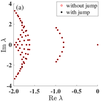
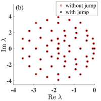
Figure 1: The Liouvillian spectrum of the Hatano-Nelson model for (a) the open boundary condition (OBC) and (b) the periodic boundary condition (PBC). The red circles represent Liouvillian without jumps, while the black dots are for full Liouvillian. We find that they are perfectly overlapping. Although our numerical calculation is restricted to have two particles at most, the observation holds for more particles. In both figures, the parameters are chosen as $J/\kappa=1$, the number of lattice site is $n=10$.

Despite the two Liouvillians hold the same spectrum, the dynamics governed by them are totally different. To be specific, in Fig. 2 we show the average particle number $N$ as a function of time $t$ with initial state $c_{1}^{\dagger}c_{2}^{\dagger}|0\rangle$ , where $|0\rangle$ is the vacuum state of fermion. The blue dash dotted line and red line in the figure are plotted for the system governed by Liouvillians with and without quantum jumps, respectively. It is obvious that the NH Hamiltonian commutes with the particle number $\left[H,N\right]=0$, so that the particle number is conserved. On the other side, the particle number decreases with time due to the quantum jumps. From these observations, we find that the same Liouvillian spectrum might leads to different dynamics because the eigenstates of the Liouvillians are different. In the other words, start from an initial state $\rho(0)$ and evolve under an non-Hermitian Hamiltonian $H_{eff}$, after a tiny time interval $\delta t$, the density matrix $\rho(\delta t)$ becomes,

$$\rho(\delta t)=\frac{e^{-iH_{eff}\delta t}\rho(0)e^{iH^{\dagger}_{eff}\delta t}}{\text{Tr}(e^{-iH_{eff}\delta t}\rho(0)e^{iH^{\dagger}_{eff}\delta t})}.$$ (11)

Clearly, the eigenergies and eigenvectors together determine the evolution of the system.

Note that we can also employ the perturbation expansion Eq. (10) to calculate $\rho(\delta t)$ and a normalization is necessary because $\rho_{n}$ in Eq. (10) are not traceless in the present perturbation theory.

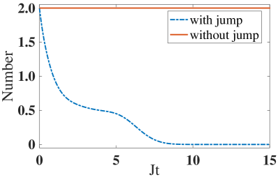
Figure 2: The average particle number as a function of time. Blue dash dotted line and red solid line stand for the Liouvillians with and without the quantum jumps.

Before closing this section, we would like to point out that our scheme is different from approximations in the literature at the following points. The first point is that we only treat the jumping terms as perturbations—this means that without perturbations the system is governed by a non-Hermitian Hamiltonian, and we focus on whether some of the results and phenomena in the various existing references are sustainable over time. And the second is that the definition of the zero-order steady state may not be so intuitive, because the zero order equation in general do not satisfies $-i(H\rho_{0}-\rho_{0}H^{\dagger})=0$, where $\rho_{0}=|r\rangle\langle l|$ and $\{|r\rangle\},\{|l\rangle\}$ is a set of right and left eigenvectors of the effective non-Hermitian Hamiltonian $H$. In our scheme the perturbation of the energy and eigenvectors of the Hamiltonian in Eq. (4) is actually used for the building of evolution equation, as shown in Eq. (10).

III application 1: TWO-LEVEL SYSTEM

In this section, we illustrate our theory with a dissipative two-level atom. We consider three decoherence channels: including the Bit-Flip and Phase-Flip channels, and their decoherence rates are $\gamma_{p}$, $\gamma_{x}$ and $\gamma_{z}$, respectively. The dynamics of the system can be described by the following master equation,

$$\dot{\rho}=-i(H\rho-\rho H^{\dagger})+\gamma_{p}\sigma_{+}\rho\sigma_{-}+\gamma_{x}\sigma_{x}\rho\sigma_{x}+\gamma_{z}\sigma_{z}\rho\sigma_{z},$$ (12)

with $H=\frac{\omega}{2}\sigma_{z}-i\frac{\gamma_{p}}{2}\sigma_{+}\sigma_{-}-i\frac{\gamma_{x}}{2}\sigma_{x}^{2}-i\frac{\gamma_{z}}{2}\sigma_{z}^{2}$, where $\sigma_{x},\sigma_{y},\sigma_{z}$ are Pauli matrix, and $\sigma_{\pm}=(\sigma_{x}\pm i\sigma_{y})/2$ are the rising and lowering operators.

Based on the effective Hamiltonian approach, we introduce an ancillary two-level system with $\sigma^{A}$ denoting its Pauli matrix. With the basis spanned by the eigenvectors of $\sigma_{z}$ and $\sigma_{z}^{A}$, with spin up state $|0\rangle$ for the system and $|0\rangle^{A}$ for the ancilla, while the spin down states are $|1\rangle$ and $|1\rangle^{A}$. We can first write out the matrix representation of $H$

$$H=\left[\begin{matrix}\frac{\omega}{2}-i\frac{\gamma_{p}}{2}-i\frac{\gamma_{x}}{2}-i\frac{\gamma_{z}}{2}&0\\ 0&-\frac{\omega}{2}-i\frac{\gamma_{x}}{2}-i\frac{\gamma_{z}}{2}\end{matrix}\right],$$ (13)

where the order of basis is $\{|0\rangle,|1\rangle\}$ and they diagonalize the Hamiltonian $H$. Apparently, ${}^{A}\langle 0|H^{A}|0\rangle^{A}=(\langle 0|H^{\dagger}|0\rangle)^{*}=\frac{\omega}{2}-i\frac{\gamma_{p}}{2}-i\frac{\gamma_{x}}{2}-i\frac{\gamma_{z}}{2}$, ${}^{A}\langle 0|H^{A}|1\rangle^{A}=(\langle 1|H^{\dagger}|0\rangle)^{*}={{}^{A}}\langle 1|H^{A}|0\rangle^{A}=(\langle 0|H^{\dagger}|1\rangle)^{*}=0$ and ${}^{A}\langle 1|H^{A}|1\rangle^{A}=(\langle 1|H^{\dagger}|1\rangle)^{*}=-\frac{\omega}{2}-i\frac{\gamma_{x}}{2}-i\frac{\gamma_{z}}{2}.$ Thus $H^{A*}$ takes

$$H^{A*}=\left[\begin{matrix}\frac{\omega}{2}+i\frac{\gamma_{p}}{2}+i\frac{\gamma_{x}}{2}+i\frac{\gamma_{z}}{2}&0\\ 0&-\frac{\omega}{2}+i\frac{\gamma_{x}}{2}+i\frac{\gamma_{z}}{2}\end{matrix}\right],$$ (14)

under its basis $\{|0\rangle^{A},|1\rangle^{A}\}$.

With the above consideration, we can obtain the matrix representation of the free Hamiltonian of the composite system $H-H^{A*}$, which will be treated as the zeroth order Hamiltonian

$$H-H^{A*}=\left[\begin{smallmatrix}-i(\gamma_{p}+\gamma_{x}+\gamma_{z})&0&0&0\\ 0&\omega-i(\frac{\gamma_{p}}{2}+\gamma_{x}+\gamma_{z})&0&0\\ 0&0&-\omega-i(\frac{\gamma_{p}}{2}+\gamma_{x}+\gamma_{z})&0\\ 0&0&0&-i(\gamma_{x}+\gamma_{z})\end{smallmatrix}\right],$$

the order of basis is $\{|0\rangle|0\rangle^{A},|0\rangle|1\rangle^{A},|1\rangle|0\rangle^{A},|1\rangle|1\rangle^{A}\}$. Similarly, the quantum jumps, i.e., the third terms in Eq. (4), which describe the coupling between the two systems read,

$$\begin{bmatrix}i\gamma_{z}&0&0&i\gamma_{x}\\ 0&-i\gamma_{z}&i\gamma_{x}&0\\ 0&i\gamma_{x}&-i\gamma_{z}&0\\ i\gamma_{p}+i\gamma_{x}&0&0&i\gamma_{z}\end{bmatrix},$$

we will treat this coupling as a perturbation. By the perturbation theory given in Eq. (II), the first and second order corrections to the eigenenergies and the right eigen-vectors can be given by,

$$\begin{split}&E^{(0)}_{1}=-i(\gamma_{p}+\gamma_{x}+\gamma_{z}),E^{(0)}_{2}=\omega-i(\frac{\gamma_{p}}{2}+\gamma_{x}+\gamma_{z}),\\ &E^{(0)}_{3}=-\omega-i(\frac{\gamma_{p}}{2}+\gamma_{x}+\gamma_{z}),E^{(0)}_{4}=-i(\gamma_{x}+\gamma_{z}).\\ &E^{(1)}_{1}=i\gamma_{z},E^{(1)}_{2}=-i\gamma_{z},E^{(1)}_{3}=-i\gamma_{z},E^{(1)}_{4}=i\gamma_{z}.\\ &E^{(2)}_{1}=\frac{-i\gamma_{x}(\gamma_{p}+\gamma_{x})}{\gamma_{p}},E^{(2)}_{2}=-\frac{\gamma_{x}^{2}}{2\omega},\\ &E^{(2)}_{3}=\frac{\gamma_{x}^{2}}{2\omega},E^{(2)}_{4}=\frac{i\gamma_{x}(\gamma_{p}+\gamma_{x})}{\gamma_{p}}.\\ &|\psi^{(1)}_{1}\rangle=-\frac{(\gamma_{p}+\gamma_{x})}{\gamma_{p}}|\psi^{(0)}_{4}\rangle,|\psi^{(1)}_{2}\rangle=\frac{i\gamma_{x}}{2\omega}|\psi^{(0)}_{3}\rangle,\\ &|\psi^{(1)}_{3}\rangle=-\frac{i\gamma_{x}}{2\omega}|\psi^{(0)}_{2}\rangle,|\psi^{(1)}_{4}\rangle=\frac{\gamma_{x}}{\gamma_{p}}|\psi^{(0)}_{1}\rangle.\\ &|\psi^{(2)}_{1}\rangle=|\psi^{(2)}_{2}\rangle=|\psi^{(2)}_{3}\rangle=|\psi^{(2)}_{4}\rangle=0.\end{split}$$ (15)

To show the validity of the perturbation theory, we present in Fig. 3 the comparison between the numerical results given by ME, NH and the perturbation theory. We find that the NH approximation is close to the numerical result in short time limit, but it gradually deviates and finally reaches its steady state, which is totally different from the steady state of the master equation. The results given by the perturbation theory are in good agreement with that given by the master equation (or the Liouvillian). Thus we can claim that the perturbation theory based on the non-Hermitian Hamiltonian might be a good method to deal with non-Hermitian systems. Of course this example is easy to solve exactly as the Hilbert space is small. In the next section, we will present a many-body system to exemplify the perturbation theory.

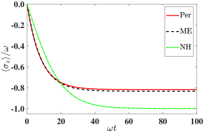
Figure 3: The average of $\sigma_{z}$ at different time $t$. The results are given by the master equation without any approximation (Per, black dashed line), non-Hermitian Hamiltonian (NH, green dash-dotted line), and the perturbation theory (ME, red solid line). The parameters chosen are $\gamma_{p}=0.1\omega,\gamma_{x}=0.01\omega,\gamma_{z}=0.5\omega$.

IV application 2: Effect of quantum jumps on the non-Hermitian BCS states

In recent years, open many-body systems become active in various fields from quantum optics to condensed matter. However the master equation of many-body open systems is difficult to solve mcdonald2021nonequilibrium ; yaoEdgeStatesTopological2018 . Here we apply our perturbation theory to such systems, taking the NH BCS model as an example yamamoto2019theory .

Due to inelastic collisions, the atoms in the BCS system suffer from two-body loss and atoms would leave the system with time, such a system can be described by an effective Markovian master equation durrliebliniger . In the case that the quantum jumps could be neglected, the earlier study yamamoto2019theory showed that when the interaction strength is not so strong, the superfluid suffer a breakdown and restoration transition occurs as the dissipation increases. Whereas in strong-dissipation limit the superfluid phase would never be broken. This gives rise to a question: what happens if the quantum jumps can not be neglected?

To answer this question concretely, we consider the 1D model in Ref. yamamoto2019theory . Here $H_{S}=\sum_{\emph{{k}}\sigma}\xi_{\emph{{k}}}c^{\dagger}_{\emph{{k}}\sigma}c_{\emph{{k}}\sigma}$ describes the free Hamiltonian of the lattice, where $\xi_{\emph{{k}}}=\epsilon_{\emph{{k}}}-\mu$, $\epsilon_{\emph{{k}}}$ stands for the energy dispersion and $\mu$ is the chemical potential. The interaction Hamiltonian $H_{I}=-U_{0}\sum_{i}c^{\dagger}_{i\uparrow}c_{i\downarrow}^{\dagger}c_{i\downarrow}c_{i\uparrow}$ (take $\hbar$=1). $c_{i\sigma}$ ($c_{\emph{{k}}\sigma}$) denote the annihilation operators of a spin-$\sigma\in\{\uparrow,\downarrow\}$ fermion at site $i$ (with momentum k). Consider the system undergoes inelastic collisions, the dynamics of the system is governed by

$$\dot{\rho}=-i(H_{\text{eff}}\rho-\rho H_{\text{eff}}^{\dagger})+\kappa\sum_{i}L_{i}\rho L_{i}^{\dagger},$$ (16)

where $\kappa$ is the loss rate and $L_{i}=c_{i\downarrow}c_{i\uparrow}$, and $H_{\text{eff}}=\sum_{\emph{{k}}\sigma}\xi_{\emph{{k}}}c^{\dagger}_{\emph{{k}}\sigma}c_{\emph{{k}}\sigma}-\sum_{\emph{{k}}\emph{{k}}^{\prime}}U_{1}/Nc^{\dagger}_{\emph{{k}}\uparrow}c^{\dagger}_{-\emph{{k}}\downarrow}c_{-\emph{{k}}^{\prime}\downarrow}c_{\emph{{k}}^{\prime}\uparrow}$. Here $N$ is the number of lattice cites and $U_{1}=U_{0}+i\kappa/2$ is the complex interaction strength.

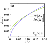
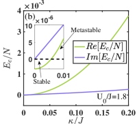
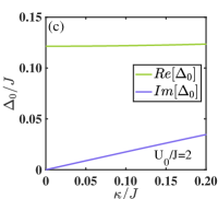
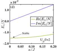
Figure 4: (a)(c) Numerical solution of non-zero superfluid gap $\delta_{0}$, (b)(d) condensation energy $E_{c}$, calculated by Eq. (18) and Eq. (22) respectively, as a function that changes with loss rate $\kappa$. Parameters are chosen as $N=10,\kappa=0.1J$, $U_{0}/J=1.8$ for (a)(b) while in (c)(d) $U_{0}/J=2$. The former system is metastable at most parameters, with stable superfluidity only in the weak dissipation limit. The latter one is always stable for strong attractive interaction $U_{0}$.

In order to diagonalize the Hamiltonian, the mean-field approximation is applied yamamoto2019theory , where the quasiparticles obey neither Fermi nor Bose statistics, since a NH Hamiltonian cannot be diagonalized by unitary transformations. Under the mean-field (MF) approximation, Hamiltonian $H_{\text{eff}}$ reduces to

$$H_{\text{MF}}=\sum_{\emph{{k}}}E_{\emph{{k}}}(\bar{\gamma}_{\emph{{k}}\uparrow}\gamma_{\emph{{k}}\uparrow}+\bar{\gamma}_{-\emph{{k}}\downarrow}\gamma_{-\emph{{k}}\downarrow})-\sum_{\emph{{k}}}E_{\emph{{k}}},$$ (17)

with $E_{\emph{{k}}}=\sqrt{\xi^{2}_{\emph{{k}}}+\Delta_{0}^{2}}$, where $\Delta_{0}=-U_{1}/N\sum_{\emph{{k}}}\langle c_{-\emph{{k}}\downarrow}c_{\emph{{k}}\uparrow}\rangle$ is the order parameter (gap function) of the superfluid. In the $\beta\rightarrow 0$ limit, the order parameter can be established with NH path integral approach yamamoto2019theory or self-consistency method fernandeslecture , which is given by the NH gap equation

$$\frac{N}{U_{1}}=\sum_{\emph{{k}}}\frac{1}{2\sqrt{\xi^{2}_{\emph{{k}}}+\Delta_{0}^{2}}},$$ (18)

when $\Delta_{0}$ takes zero, such phase is denoted as “normal state”, where the gap equation has only a trivial solution. For most cases $\Delta_{0}$ is a complex number.

The quasiparticle operators in Eq. (17) can be written as

$$\bar{\gamma}_{\emph{{k}}\uparrow}=u_{\emph{{k}}}c^{\dagger}_{\emph{{k}}\uparrow}-v_{\emph{{k}}}c_{-\emph{{k}}\downarrow},\bar{\gamma}_{-\emph{{k}}\downarrow}=v_{\emph{{k}}}c_{\emph{{k}}\uparrow}+u_{\emph{{k}}}c^{\dagger}_{-\emph{{k}}\downarrow},$$ (19)

$$\gamma_{\emph{{k}}\uparrow}=u_{\emph{{k}}}c_{\emph{{k}}\uparrow}-v_{\emph{{k}}}c^{\dagger}_{-\emph{{k}}\downarrow},\gamma_{-\emph{{k}}\downarrow}=v_{\emph{{k}}}c^{\dagger}_{\emph{{k}}\uparrow}+u_{\emph{{k}}}c_{-\emph{{k}}\downarrow},$$ (20)

with $u_{\emph{{k}}}=\sqrt{\frac{E_{\emph{{k}}}+\xi_{\emph{{k}}}}{2E_{\emph{{k}}}}}$, $v_{\emph{{k}}}=\sqrt{\frac{E_{\emph{{k}}}-\xi_{\emph{{k}}}}{2E_{\emph{{k}}}}}$. In the above derivation, the symmetry $H_{\text{MF}}^{*}=H_{\text{MF}}^{\dagger}$ has been used, which could be found from the matrix representation in terms of Fock states. In fact, under such representation, the non-Hermiticity of the system attributes to the complex diagonal elements, which implies that the left eigenvector $|L_{n}\rangle$ of the Hamiltonian is exactly the complex conjugation of right one $|R_{n}\rangle$ yamamoto2019theory .

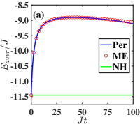
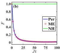
Figure 5: (a) The average energy $E_{aver}=\langle H_{S}\rangle$ and (b) the fidelity of initial state governed by perturbation method (blue solid line), master equation (red circles) and non-Hermitian Hamiltonian (green solid line), respectively. Here we take $\epsilon_{\emph{{k}}}=-2J\cos{\emph{{k}}}$, here $J$ is the hopping amplitude, and the loss rate $\kappa$ is set to be $0.1J$ and $\mu=0$. The interaction strength is set to be $U_{0}=1.8J$, the number of lattice sites $N$ takes 10. The order parameter $\Delta_{0}/J=0.0786+0.0777i$ (obtained by solving Eq. (18)), and the system is assume to stay in the superfluid state (metastable).

In the following discussion, we would focus on the ground state of the system. To clarify the discussion, we write down the right and left ground state,

$$|r_{0}\rangle = |BCS\rangle_{R}=\prod_{\emph{{k}}}(u_{\emph{{k}}}+v_{\emph{{k}}}c^{\dagger}_{\emph{{k}}\uparrow}c^{\dagger}_{-\emph{{k}}\downarrow})|0\rangle,$$

$$|l_{0}\rangle = |BCS\rangle_{L}=\prod_{\emph{{k}}}(u^{*}_{\emph{{k}}}+v^{*}_{\emph{{k}}}c^{\dagger}_{\emph{{k}}\uparrow}c^{\dagger}_{-\emph{{k}}\downarrow})|0\rangle,$$ (21)

where $|0\rangle$ is the vacuum state of the fermions. It is easy to find that $H\bar{\gamma}_{\emph{{k}}\sigma}|BCS\rangle_{R}=E_{\emph{{k}}}\bar{\gamma}_{\emph{{k}}\sigma}|BCS\rangle_{R},H^{\dagger}{\gamma}^{\dagger}_{\emph{{k}}\sigma}|BCS\rangle_{L}=E^{*}_{\emph{{k}}}{\gamma}^{\dagger}_{\emph{{k}}\sigma}|BCS\rangle_{L}.$ Here $H$ is Hamiltonian $H_{MF}$ except the constant $-\sum_{\emph{{k}}}E_{\emph{{k}}}$ is neglected. In this way, all left and right eigenvectors $\{|l_{n}\rangle\},\{|r_{n}\rangle\}$ of the effective Hamiltonian $H$ can be constructed.

In Hermitian case, the superfluidity of the system arises from the non-zero gap function, since the energy spectrum will always have a gap in order to excite quasiparticles, even if $\xi_{\emph{{k}}}$ takes $0$ fernandeslecture . However, for NH systems, such defined superfluid may be metastable, distinguished by the sign of the real part of the condensation energy $E_{c}$

$$E_{c}=\frac{N}{U_{1}}\Delta_{0}^{2}-\sum_{\emph{{k}}}(\sqrt{\xi^{2}_{\emph{{k}}}+\Delta_{0}^{2}}-|\xi_{\emph{{k}}}|),$$ (22)

actually, $E_{c}$ represents the difference in the ground-state energy between the superfluid and normal states. For positive $\text{Re}(E_{c})$, the system is metastable, while a negative $\text{Re}(E_{c})$ leads to a stable superfluid solution yamamoto2019theory . Fig. 4-4 show real and imaginary part of the gap function $\Delta_{0}$ and the condensation energy $E_{c}$ when $U_{1}=1.8J$ and $2J$, respectively. Apparently, the NH gap equations have nontrivial solutions, for small $U_{0}$, the system is stable only at the small dissipation limit. As attractive interaction strength $U_{0}$ gets stronger, the system remains stable.

In order to analyse the jump involved circumstance, suppose the system is initially prepared in a NH steady state $\rho_{0},$ satisfying $\dot{\rho}_{0}=-i(H_{\text{eff}}\rho_{0}-\rho_{0}H_{\text{eff}}^{\dagger})=0$ and $\text{Tr}(\rho_{0})=1$. Clearly we can choose $\rho_{0}=\mathcal{N}|r_{0}\rangle\langle r_{0}|$ as an initial state that meets the requirement. Here $\mathcal{N}$ is the normalization coefficient that satisfies $\text{Tr}(\rho_{0})=\sum_{n}\langle l_{n}|\rho_{0}|r_{n}\rangle=1$. Now we apply the perturbation theory into the NH BCS system. Consider that our system has only two-body loss, we then restrict the Hilbert space enclosing at most 2 quasiparticles. The corresponding eigenergies are (the constant in Eq. (17) is omitted) $\{0,0-2E_{\emph{{k}}_{1}}^{*},0-2E_{\emph{{k}}_{2}}^{*}\dots,2E_{\emph{{k}}_{1}}-0,2E_{\emph{{k}}_{1}}-2E_{\emph{{k}}_{1}}^{*}\dots,\dots,2E_{\emph{{k}}_{n}}-0,2E_{\emph{{k}}_{n}}-2E_{\emph{{k}}_{1}}^{*}\dots,2E_{\emph{{k}}_{n}}-2E_{\emph{{k}}_{1}}^{*}\}$. In this Hilbert space, the matrix representation of the quantum jumps $L_{\emph{{k}}_{0}}$ takes

$$\begin{bmatrix}u_{\emph{{k}}_{0}}v_{\emph{{k}}_{0}}&0&\cdots&u_{\emph{{k}}_{0}}^{2}&\cdots&0\\ 0&u_{\emph{{k}}_{0}}v_{\emph{{k}}_{0}}&\cdots&0&\cdots&0\\ \vdots\ &\vdots&\ddots&\vdots&\cdots&0\\ -v_{\emph{{k}}_{0}}^{2}&0&\cdots&-u_{\emph{{k}}_{0}}v_{\emph{{k}}_{0}}&\cdots&0\\ \vdots&\vdots&\vdots&\vdots&\ddots&0\\ 0&0&\cdots&0&\dots&u_{\emph{{k}}_{0}}v_{\emph{{k}}_{0}}\end{bmatrix},$$ (23)

here the order of the basis is arranged as $\{|r_{0}\rangle,\bar{\gamma}_{\emph{{k}}_{1}\uparrow}\bar{\gamma}_{-\emph{{k}}_{1}\downarrow}|r_{0}\rangle,\\ \dots,\bar{\gamma}_{\emph{{k}}_{n}\uparrow}\bar{\gamma}_{-\emph{{k}}_{n}\downarrow}|r_{0}\rangle\}\{\langle l_{0}|,\langle l_{0}|\gamma^{\dagger}_{-\emph{{k}}_{1}\downarrow}\gamma^{\dagger}_{\emph{{k}}_{1}\uparrow},\dots,\langle l_{0}|\gamma^{\dagger}_{-\emph{{k}}_{n}\downarrow}\gamma^{\dagger}_{\emph{{k}}_{n}\uparrow}\}$. Notice that the diagonal elements with a minus sign result from the contribution of $\bar{\gamma}_{\emph{{k}}_{0}\uparrow}\bar{\gamma}_{-\emph{{k}}_{0}\downarrow}|r_{0}\rangle,\langle l_{0}|\gamma^{\dagger}_{-\emph{{k}}_{0}\downarrow}\gamma^{\dagger}_{\emph{{k}}_{0}\uparrow}$.

By the definition given in Eq. (4), the first two terms $H-H^{A*}$ can be taken as zero-order Hamiltonian and the third term $i\sum_{m}\kappa_{m}F_{m}F^{A*}_{m}$ is the perturbation. Collecting the results in yamamoto2019theory , we find that the zeroth energy of the ground state is

$$E^{(0)}_{0}=-2\sum_{\emph{{k}}}\text{Im}(E_{\emph{{k}}}),$$ (24)

by the non-Hermitian perturbation theory, the first order correction to the energy of the ground state is given by

$$E^{(1)}_{0}=-\kappa\sum_{\emph{{k}}}|u_{\emph{{k}}}|^{2}|v_{\emph{{k}}}|^{2}.$$ (25)

Here we want to emphasize that the complex constant eigenenergy of the system can be safely ignored, similar to Hermitian systems that constants can not affect their dynamical features. This can be interpreted as a gauge shift $H\rightarrow H+cI$, where $I$ is the identity operator and $c$ is a complex c-number. In other words, the dynamics under $H$ and $H+cI$ is the same zloshchastiev2014comparisona . By our theory, the first order corrections to the left and right ground states are (unnormalized)

$$|r_{0}^{(1)}\rangle=\sum_{\emph{{k}}}\frac{-i\kappa u_{\emph{{k}}}v_{\emph{{k}}}v_{\emph{{k}}}^{*2}}{2E_{\emph{{k}}}^{*}}|r_{0}\rangle\gamma^{\dagger}_{{\emph{{k}}}\uparrow}\gamma^{\dagger}_{-{\emph{{k}}}\downarrow}|l_{0}\rangle+\sum_{\emph{{k}}}\frac{i\kappa u_{\emph{{k}}}^{*}v_{\emph{{k}}}^{*}v^{2}_{\emph{{k}}}}{2E_{\emph{{k}}}}\bar{\gamma}_{\emph{{k}}\uparrow}\bar{\gamma}_{-\emph{{k}}\downarrow}|r_{0}\rangle|l_{0}\rangle-\sum_{\emph{{k}}}\frac{\kappa|v_{\emph{{k}}}|^{4}}{4\text{Im}(E_{\emph{{k}}})}\bar{\gamma}_{\emph{{k}}\uparrow}\bar{\gamma}_{-\emph{{k}}\downarrow}|r_{0}\rangle\gamma^{\dagger}_{{\emph{{k}}}\uparrow}\gamma^{\dagger}_{-{\emph{{k}}}\downarrow}|l_{0}\rangle,$$ (26)

$$|l^{(1)}_{0}\rangle=\sum_{\emph{{k}}}\frac{-i\kappa u^{*}_{{\emph{{k}}}}v_{{\emph{{k}}}}^{*}v_{{\emph{{k}}}}^{2}}{2E_{{\emph{{k}}}}}|l_{0}\rangle\bar{\gamma}_{{\emph{{k}}}\uparrow}\bar{\gamma}_{-{\emph{{k}}}\downarrow}|r_{0}\rangle+\sum_{\emph{{k}}}\frac{i\kappa u^{*2}_{\emph{{k}}}u_{\emph{{k}}}v_{\emph{{k}}}}{2E_{\emph{{k}}}^{*}}\gamma^{\dagger}_{{\emph{{k}}}\uparrow}\gamma^{\dagger}_{-{\emph{{k}}}\downarrow}|l_{0}\rangle|r_{0}\rangle-\sum_{\emph{{k}}}\frac{\kappa|v_{\emph{{k}}}|^{4}}{4\text{Im}(E_{\emph{{k}}})}\gamma^{\dagger}_{{\emph{{k}}}\uparrow}\gamma^{\dagger}_{-{\emph{{k}}}\downarrow}|l_{0}\rangle\bar{\gamma}_{{{\emph{{k}}}\uparrow}}\bar{\gamma}_{{-{\emph{{k}}}\downarrow}}|r_{0}\rangle.$$

The normalization condition is $|\mathcal{N}_{0}|^{2}(\langle l^{(0)}_{0}|+\langle l^{(1)}_{0}|)(|r^{(0)}_{0}\rangle+|r^{(1)}_{0}\rangle)=1$, where $\mathcal{N}_{0}$ is the normalization constant of the right ground state. Simple algebra yields $|\mathcal{N}_{0}|^{2}=1/(\sum_{\emph{{k}}}\frac{\kappa^{2}|u_{\emph{{k}}}|^{4}|v_{\emph{{k}}}|^{4}}{4E_{\emph{{k}}}^{*2}}+\sum_{\emph{{k}}}\frac{\kappa^{2}|u_{\emph{{k}}}|^{4}|v_{\emph{{k}}}|^{4}}{4E_{\emph{{k}}}^{2}}+\sum_{\emph{{k}}}\frac{\kappa^{2}|u_{\emph{{k}}}|^{4}|v_{\emph{{k}}}|^{4}}{16\text{Im}(E_{\emph{{k}}})^{2}}+1)$. The first order corrections to the other eigenvectors can be computed in the same way. These eigenvectors form a new biorthonormal and complete basis, and the whole dynamic can be predicted by Eq. (10). The calculations is tedious and expression is involved, so we do not present them here.

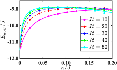
Figure 6: The average energy $E_{aver}$ as a function of loss rate $\kappa$ at different time $t$. We calculate this energy by both the master equation (solid lines) and the perturbation theory (dotted lines). The purple solid line, red dashed line, blue dotted line, green dash dotted line and cyan solid line are for different times, $Jt=10,20,30,40,50$, respectively. Parameter $U_{0}=1.8J$ and the number of lattice sites is 10.

In Fig. 5, we plot the average energy of the system at time $t$. The results are given by first order perturbation (blue solid line) and by numerical simulations with the master equation (red circles). For the comparison purpose, the results given by non-Hermitian Hamiltonian (green solid line) are also shown. We can find that the results given by perturbation theory match well with that by the master equation even for long time evolution. The other interesting observation is that the energy has a large degree of deviation from the prediction based on the non-Hermitian Hamiltonian. Remind that energy by non-Hermitian evolution is always unchanged because the initial state (i.e., the ground state) is a steady state of the system. This feature can be understood by examining the fidelity of ground state $F=|\text{Tr}(\rho_{0}\rho)|/\sqrt{\text{Tr}(\rho_{0}^{2})\text{Tr}(\rho^{2})}$ wang2008alternative . As showed in Fig. 5, at $Jt=100$ the system is almost all excited to the excited states, resulting in a low fidelity between the initial states. This result suggests that the quantum jumps play an important role in this system, and the state $|r_{0}\rangle$ is unstable under the effect of quantum jumps.

From the other point of view, non-Hermitian BCS model does not conserve the number of fermions and thus the Liouvillians without and with quantum jumps can not be written into a block-diagonal and block-upper-triangular form, respectively. This leads to different spectrum for the Liouvillians with and without quantum jumps yoshida2020fate ; torres2014closedform . This observation is quite different from that of the non-Hermitian Hatano-Nelson model. From the view point of quasiparticle, the quasiparticle number conserves because $\left[H_{MF},\sum_{\emph{{k}}\sigma}\bar{\gamma}_{\emph{{k}}\sigma}\gamma_{\emph{{k}}\sigma}\right]=0$. However, in the basis spanned by the quasiparticles, the jumping terms $\sum_{\emph{{k}}}\kappa c_{-\emph{{k}}\downarrow}c_{\emph{{k}}\uparrow}$ still can not be written as block-upper-triangular form, which is in agreement with the aforementioned analysis.

In Fig. 6, we perform a comparison between the results of the master equation and by the first order perturbation with different loss rate $\kappa$. We observe that the bigger the loss rate is, the more intensity the excitation will be at the beginning. Moreover, even when $\kappa$ is small, after long time, the average energy of the system suffers abruptly change. As $\kappa$ increase, the whole dynamic is totally different from NH ones (The same property as the green solid in Fig. 5).

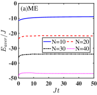
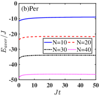
Figure 7: The time evolution of average energy $E_{aver}$ for different $N$. $U_{0}=1.8J$ and the loss rate $\kappa=0.05J$ were set for these plots. (a) are the results from the master equation, and (b) are the corresponding results from the perturbation theory. The blue solid line, red dashed line, black dash-dotted line and cyan dotted line represent $N=10,20,30,40$ respectively.

Fig. 7 and 7 shows the time evolution of the average energy with different system sizes. The results are calculated with both the master equation and the perturbation theory. The fact is that the two results (one from the master equation while another from the perturbation theory) matches well even for system of big size suggest the validity of the our theory, which is also essential in many-body systems.

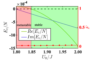
Figure 8: Left axis: condensation energy $E_{c}$ as a function of $U_{1}/J$, $\kappa/J=0.1$, as $U_{1}/J$ increases, the superfluid undergoes a phase transition, from metastable area (red) to stable area (green). Right axis: fidelity of ground state at time $Jt=50$, the red solid line represent ME simulation, while the red dots stand for the perturbation, there is no significant difference in system dynamics.

Finally, we consider the condensation energy $E_{c}$ of the effective model that changes with the interaction strength $U_{0}$, with a fixed loss rate $\kappa=0.1J$, as shown in Fig. 8. As $U_{0}$ increases from $1.8J$ (as in Fig. 4) to $2J$ (as in Fig. 4), the real part of $E_{c}$ crosses the zero point, which leads to the transition of the superfluidity from the metastable (red area) to the stable region (green area). Similar result is also addressed in Ref. yamamoto2019theory . However, at $Jt=50$, when quantum jumps are introduced, there is no significant variation in the fidelity $F$ from the ground state. It illustrates that in the study of NH systems, the presence of quantum jump events may challenge certain properties of NH systems, which warrants further investigation. Our proposed method can serve as a solid foundation for such research and verification.

V CONCLUSION

Based on the effective Hamiltonian approach, we developed a perturbation theory to study open quantum systems governed by the Lindblad master equation. Treating the quantum jumps as perturbations, we derived a set of corrections up to the first and second order in the jumps to the eigenenergies and corresponding eigenfunctions. This development is not trivial since our perturbation theory is based on the non-Hermitian Hamiltonian and then the basis of the Hilbert space behaves differently from its Hermitian counterpart. We applied our theory to two examples, a decoherence two-level system and the non-Hermitian BCS model. The results show that the present theory is in good agreement with the results obtained by solving the master equation. Besides, the present theory saves the computing time and in most cases analytical expressions can be found. We believe that the present theory opens a door to study the non-Hermitian physics and pave a way to check the validity of the description of open systems by non-Hermitian Hamiltonians.

Appendix A THE DERIVATION OF EFFECTIVE HAMILTONIAN APPROACH

In this appendix, we will introduce the effective Hamiltonian approach, which was proposed to exactly solve the master equation of open quantum systems.

According to the master equation Eq. (1), the differential equation of matrix element $\rho_{mn}=\langle l_{m}|\rho|l_{n}\rangle$ can be written as

$$i\dot{\rho}_{mn}=\sum_{mn}\langle l_{m}|(H\rho-\rho H^{\dagger}+i\kappa F\rho F^{\dagger})|l_{n}\rangle,$$ (27)

where $H=H_{0}-i\kappa/2F^{\dagger}F$ is the effective non-Hermitian Hamiltonian.

For simplicity we assume that there is only one Lindblad operator in the master equation Eq. (1). We introduce an auxiliary system A (the ancilla, which is the same as the system), and then extend the $N$-dimensional Hilbert space to an $N^{2}$-dimensional Hilbert space. The Hilbert space of the composite system (the open quantum system plus the ancilla) can be expanded by a set of biorthonormal basis $\{|l_{m}\rangle\otimes|L_{n}\rangle^{A*},\,|r_{m}\rangle\otimes|R_{n}\rangle^{A*}\}$, where $|R_{n}\rangle^{A}$ and $|L_{n}\rangle^{A}$ are the right and left basis for the ancilla Hilbert space. At this time, a density matrix $\rho$ of the open quantum system can be mapped into a pure bipartite state in $N^{2}$-dimensional Hilbert space, i.e.,

$$|\psi_{\rho}(t)\rangle=\sum^{N}_{mn}\rho_{mn}(t)|r_{m}\rangle|R_{n}\rangle^{A*}.$$ (28)

Taking the time derivative on the pure state $|\psi_{\rho}(t)\rangle$, it yields

$$i\partial_{t}|\psi_{\rho}(t)\rangle=\sum^{N}_{mn}\left(\langle l_{m}|(H\rho-\rho H^{\dagger}+i\kappa F\rho F^{\dagger})|l_{n}\rangle\right)|r_{m}\rangle|R_{n}\rangle^{A*}.$$ (29)

For an arbitrary system operator $O$, we can define a corresponding operator $O^{A}$ of the ancilla, which satisfies $\langle r_{m}|O^{\dagger}|l_{n}\rangle=(^{A}\langle L_{n}|O^{A}|R_{m}\rangle^{A})^{*}$. Inserting the complete relation Eq. (3) into Eq. (29), it is not difficult to obtain

$$\sum_{mn}\langle l_{m}|H\rho|l_{n}\rangle|r_{m}\rangle|R_{n}\rangle^{A*} = H\otimes I^{A}|\psi_{\rho}(t)\rangle,$$

$$\sum_{mn}\langle l_{m}|\rho H^{\dagger}|l_{n}\rangle|r_{m}\rangle|R_{n}\rangle^{A*} = I\otimes(H^{A})^{*}|\psi_{\rho}(t)\rangle,$$

$$\sum_{mn}\langle l_{m}|F\rho F^{\dagger}|l_{n}\rangle|r_{m}\rangle|R_{n}\rangle^{A*} = F\otimes(F^{A})^{*}|\psi_{\rho}(t)\rangle.$$

Thus, the dynamical equation for the composite system can be rewritten as

$$i\partial_{t}|{\psi}_{\rho}(t)\rangle=\widetilde{H}|\psi_{\rho}(t)\rangle,$$ (30)

with the effective Hamiltonian $\widetilde{H}=H\otimes I-I\otimes(H^{A})^{*}+i\kappa F\otimes(F^{A})^{*}.$ Therefore, the master equation is equivalent to the evolution of a pure state of the composite system. The jumping terms in the master equation describe the interactions between the open quantum system and the ancilla. More, if we choose the basis of the ancilla the same representation as the system, the effective Hamiltonian returns to the Liouvillian superoperator ( a $-i$ factor is neglected) minganti2019quantum ,

$$\widetilde{H}=(H_{0}-\frac{i\kappa F^{\dagger}F}{2})\otimes I-I\otimes(H_{0}^{\text{TR}}+\frac{i\kappa F^{\text{TR}}F^{*}}{2})+i\kappa F\otimes F^{*},$$ (31)

where TR denotes transpose operation.

Appendix B A SHORT DERIVATION OF THE EQUIVALENCE OF BIORTHOGONAL BASIS

Consider an arbitrary non-Hermitian system with a Hamiltonian $H_{NH}$ which is diagonalizable and nondegenerate. The biorthonormal basis $\{|r_{n}\rangle\},\{|l_{n}\rangle\}$ are the right and left eigenvectors of $H_{NH}$, which satisfy Eq. (2). In the following, we divide our discussion into two cases, i.e., the real spectrum and the complex spectrum wang1979disscussion .

Now we first prove that $H_{NH}$ with a real spectrum $\{E_{n}\}$ can be written as $H_{NH}=(A^{-1})^{\dagger}H_{H}A^{\dagger}$, where $H_{H}$ is a Hermitian Hamiltonian and $A$ is a non-unitary operator.According to the completeness relation $\langle l_{n}|r_{m}\rangle=\delta_{mn}$, the left eigenvector $|l_{n}\rangle$ can be expressed as an expansion of the right eigenvetors, i.e.,

$$|l_{n}\rangle=\sum_{n^{\prime}}M_{nn^{\prime}}|r_{n^{\prime}}\rangle,$$ (32)

taking an Hermitian conjugate operation on above equation and acting $|r_{n^{\prime}}\rangle$ on the result from the right hand side, it yields

$$\langle l_{n}|r_{n^{\prime}}\rangle=\sum_{n^{\prime\prime}}M^{*}_{nn^{\prime\prime}}\langle r_{n^{\prime\prime}}|r_{n^{\prime}}\rangle=\delta_{nn^{\prime}}.$$ (33)

From Eq. (33), it is easy to obtain $(M^{*})X=I$, where $X_{mn}=\langle r_{m}|r_{n}\rangle$ and $I$ is the identity matrix. Thus

$$(M^{*-1})_{mn}=\langle r_{m}|r_{n}\rangle,$$ (34)

$$(M^{-1})_{mn}=\langle r_{n}|r_{m}\rangle.$$ (35)

Combing Eq. (34) and (35), it is straightforward to find that $(M^{*-1})_{nm}=(M^{-1})_{mn}$ always holds for arbitrary $m,n$. Recall the definition of the Hermitian matrix, $M^{-1}$ is a Hermitian matrix, which implies that $M$ is Hermitian. In other words, the left eigenvectors $\{|l_{n}\rangle\}$ can be obtained from the right eigenvectors $\{|r_{n}\rangle\}$ via a Hermitian transformation. Considering an arbitrary set of complete orthonormal basis $\{|{n}\rangle\}$, we have $(M^{-1})_{nm}=\langle r_{n}|r_{m}\rangle=\sum_{n^{\prime}}\langle r_{n}|{n^{\prime}}\rangle\langle{n^{\prime}}|r_{m}\rangle=(A^{\dagger-1}A^{-1})_{nm}\!$. By defining $(A^{\dagger-1})_{nn^{\prime}}=\langle r_{n}|{n^{\prime}}\rangle$, it can be seen that

$$U=AA^{\dagger},$$ (36)

as a result, we obtain Eq. (7) from Eq. (36) and Eq. (32).

For a non-Hermitian $H_{NH}$ with a complex energy spectrum $\{E_{n}\}$, we can always find two Hermitian Hamiltonian $H_{1}=H_{1}^{\dagger}$, $H_{2}=H_{2}^{\dagger}$ which satisfy $H_{NH}=H_{1}+iH_{2}$. We still have two cases such as $H_{NH1}:\left[H_{1},H_{2}\right]\!=\!0$ and $H_{NH2}:\left[H_{1},H_{2}\right]\!\neq\!0$ . For the former situation, despite the $H_{NH}$ is non-Hermitian, $H_{1}$ and $H_{2}$ share common orthonormal basis $\{|n\rangle\}$. For the latter case, it can be proved that $H_{NH2}$ is of an equivalence relation with $H_{NH1}$. According to Eq. (36), we have $|l_{n}\rangle=U|r_{n}\rangle=AA^{\dagger}|r_{n}\rangle$ and $A^{-1}|l_{n}\rangle=A^{\dagger}|r_{n}\rangle=|n\rangle$. $\{|n\rangle\}$ is a set of orthonormal basis which relate to a non-Hermitian Hamiltonian $H_{NH1}$. Thus, it yields $A^{\dagger}H_{NH2}(A^{\dagger})^{-1}|n\rangle=E_{n}|n\rangle$ and $A^{-1}H_{NH2}A|n\rangle=E_{n}^{*}|n\rangle$. Therefore, Eq. (7) always holds.

References

- [1] Carl M. Bender. Making Sense of Non-Hermitian Hamiltonians. Reports on Progress in Physics, 70(6):947–1018, 2007.
- [2] Yuto Ashida, Zongping Gong, and Masahito Ueda. Non-Hermitian Physics. Advances in Physics, 69(3):249–435, 2020.
- [3] Zhihao Xu and Shu Chen. Topological Bose-Mott insulators in one-dimensional non-Hermitian superlattices. Physical Review B, 102(3):035153, 2020.
- [4] Tao Liu, James Jun He, Tsuneya Yoshida, Ze-Liang Xiang, and Franco Nori. Non-Hermitian topological Mott insulators in one-dimensional fermionic superlattices. Physical Review B, 102(23):235151, 2020.
- [5] Shunyu Yao and Zhong Wang. Edge States and Topological Invariants of Non-Hermitian Systems. Physical Review Letters, 121(8):086803, 2018.
- [6] Tony E. Lee and Ching-Kit Chan. Heralded Magnetism in Non-Hermitian Atomic Systems. Physical Review X, 4(4):041001, 2014.
- [7] Tsuneya Yoshida, Koji Kudo, and Yasuhiro Hatsugai. Non-Hermitian fractional quantum Hall states. Scientific Reports, 9(1):16895, 2019.
- [8] José A. S. Lourenço, Ronivon L. Eneias, and Rodrigo G. Pereira. Kondo effect in a PT -symmetric non-Hermitian Hamiltonian. Physical Review B, 98(8):085126, 2018.
- [9] M.V. Berry. Physics of Nonhermitian Degeneracies. Czechoslovak Journal of Physics, 54(10):1039–1047, 2004.
- [10] Absar U. Hassan, Bo Zhen, Marin Soljačić, Mercedeh Khajavikhan, and Demetrios N. Christodoulides. Dynamically Encircling Exceptional Points: Exact Evolution and Polarization State Conversion. Physical Review Letters, 118(9):093002, 2017.
- [11] Weijian Chen, Şahin Kaya Özdemir, Guangming Zhao, Jan Wiersig, and Lan Yang. Exceptional points enhance sensing in an optical microcavity. Nature, 548(7666):192–196, 2017.
- [12] Yu Hung Lai, Yu Kun Lu, Myoung Gyun Suh, Zhiquan Yuan, and Kerry Vahala. Observation of the exceptional-point-enhanced Sagnac effect. Nature, 576(7785):65–69, 2019.
- [13] Taiki Haga, Masaya Nakagawa, Ryusuke Hamazaki, and Masahito Ueda. Liouvillian Skin Effect: Slowing Down of Relaxation Processes without Gap Closing. Physical Review Letters, 127(7):070402, 2021.
- [14] Eunwoo Lee, Hyunjik Lee, and Bohm Jung Yang. Many-body approach to non-Hermitian physics in fermionic systems. Physical Review B, 101(12):121109, 2020.
- [15] Nobuyuki Okuma, Kohei Kawabata, Ken Shiozaki, and Masatoshi Sato. Topological Origin of Non-Hermitian Skin Effects. Physical Review Letters, 124(8):086801, 2020.
- [16] Xiao-Ran Wang, Cui-Xian Guo, and Su-Peng Kou. Defective edge states and number-anomalous bulk-boundary correspondence in non-Hermitian topological systems. Physical Review B, 101(12):121116, 2020.
- [17] Chen Shen, Junfei Li, Xiuyuan Peng, and Steven A. Cummer. Synthetic exceptional points and unidirectional zero reflection in non-Hermitian acoustic systems. Physical Review Materials, 2(12):125203, 2018.
- [18] Cong Hua Yan, Ming Li, Xin Biao Xu, Yan Lei Zhang, Hao Yuan, and Chang Ling Zou. Unidirectional transmission of single photons under nonideal chiral photon-atom interactions. Physical Review Letters, 127, 140504, 2020
- [19] Dorje C Brody. Biorthogonal quantum mechanics. Journal of Physics A: Mathematical and Theoretical, 47(3):035305, 2014.
- [20] Kazuki Yamamoto, Masaya Nakagawa, Kyosuke Adachi, Kazuaki Takasan, Masahito Ueda, and Norio Kawakami. Theory of Non-Hermitian Fermionic Superfluidity with a Complex-Valued Interaction. Physical Review Letters, 123(12):123601, 2019.
- [21] Kang Yang, Siddhardh C. Morampudi, and Emil J. Bergholtz. Exceptional Spin Liquids from Couplings to the Environment. Physical Review Letters, 126(7):077201, 2021.
- [22] Zongping Gong, Yuto Ashida, Kohei Kawabata, Kazuaki Takasan, Sho Higashikawa, and Masahito Ueda. Topological Phases of Non-Hermitian Systems. Physical Review X, 8(3):031079, 2018.
- [23] Yu Xin Wang and A. A. Clerk. Non-Hermitian dynamics without dissipation in quantum systems. Physical Review A, 99(6):063834, 2019.
- [24] S Dürr, J J García-Ripoll, N Syassen, D M Bauer, M Lettner, J I Cirac, and G Rempe. Lieb-Liniger model of a dissipation-induced Tonks-Girardeau gas. Physical Review A, 79(2):13, 2009.
- [25] Fabrizio Minganti, Adam Miranowicz, Ravindra W. Chhajlany, and Franco Nori. Quantum exceptional points of non-Hermitian Hamiltonians and Liouvillians: The effects of quantum jumps. Physical Review A, 100(6):062131, 2019.
- [26] Weijian Chen, Maryam Abbasi, Yogesh N. Joglekar, and Kater W. Murch. Quantum jumps in the non-Hermitian dynamics of a superconducting qubit. Physical Review Letters, 127, 140504, 2021.
- [27] Fabrizio Minganti, Adam Miranowicz, Ravindra W. Chhajlany, Ievgen I. Arkhipov, and Franco Nori. Hybrid-Liouvillian formalism connecting exceptional points of non-Hermitian Hamiltonians and Liouvillians via postselection of quantum trajectories. Physical Review A, 101(6):062112, 2020.
- [28] Klaus Mølmer, Yvan Castin, and Jean Dalibard. Monte Carlo wave-function method in quantum optics. Journal of the Optical Society of America B, 10(3):524, 1993.
- [29] Jean Dalibard, Yvan Castin, and Klaus Mølmer. Wave-function approach to dissipative processes in quantum optics. Physical Review Letters, 68(5):580–583, 1992.
- [30] Andrew J. Daley. Quantum trajectories and open many-body quantum systems. Advances in Physics, 63(2):77–149, 2014.
- [31] X X Yi and S X Yu. Effective hamiltonian approach to the master equation. Journal of Optics B: Quantum and Semiclassical Optics, 3(6):372, 2001.
- [32] Tosio Kato. Perturbation theory for linear operators, volume 132. Springer Science & Business Media, 2013.
- [33] Morton M. Sternheim and James F. Walker. Non-Hermitian Hamiltonians, Decaying States, and Perturbation Theory. Physical Review C, 6(1):114–121, 1972.
- [34] J. Bardeen, L. N. Cooper, and J. R. Schrieffer. Microscopic Theory of Superconductivity. Physical Review, 106(1):162–164, 1957.
- [35] Crispin Gardiner, Peter Zoller, and Peter Zoller. Quantum noise: a handbook of Markovian and non-Markovian quantum stochastic methods with applications to quantum optics. Springer Science & Business Media, 2004.
- [36] B. Kraus, H. P. Büchler, S. Diehl, A. Kantian, A. Micheli, and P. Zoller. Preparation of entangled states by quantum Markov processes. Physical Review A, 78(4):042307, 2008.
- [37] D. F. Walls, M. J. Collet, and G. J. Milburn. Analysis of a quantum measurement. Physical Review D, 32(12):3208–3215, 1985.
- [38] Frank Verstraete, Michael M. Wolf, and J. Ignacio Cirac. Quantum computation and quantum-state engineering driven by dissipation. Nature Physics, 5(9):633–636, 2009.
- [39] Ji Il Kim, M. C. Nemes, A. F. R. toledo pizade Toledo Piza, and H. E. Borges. Perturbative Expansion for Coherence Loss. Physical Review Letters, 77(2):207–210, 1996.
- [40] X. X. Yi, C. Li, and J. C. Su. Perturbative expansion for the master equation and its applications. Physical Review A, 62(1):013819, 2000.
- [41] Andy C. Y. Li, F. Petruccione, and Jens Koch. Perturbative approach to Markovian open quantum systems. Scientific Reports, 4(1):4887, 2015.
- [42] Li, A. C. Y., Petruccione, F., and Koch, J. Resummation for Nonequilibrium Perturbation Theory and Application to Open Quantum Lattices. Phys. Rev. X, 6 (2), 021037, 2016
- [43] Albert, Victor V. Lindbladians with multiple steady states: theory and applications arXiv:1802.00010, 2018.
- [44] Heinz Peter Breuer, Francesco Petruccione, et al. The theory of open quantum systems. Oxford University Press on Demand, 2002.
- [45] G. Lindblad. On the generators of quantum dynamical semigroups. Communications in Mathematical Physics, 48(2):119–130, 1976.
- [46] Qi Zhang and Biao Wu. Non-Hermitian quantum systems and their geometric phases. Physical Review A, 99(3):032121.
- [47] Carl M. Bender and Gerald V. Dunne. Large-order Perturbation Theory for a Non-Hermitian PT-symmetric Hamiltonian. Journal of Mathematical Physics, 40(10):4616–4621, 1999.
- [48] Doru Sticlet, Balázs Dóra, and Cătălin Paşcu Moca. Kubo Formula for Non-Hermitian Systems and Tachyon Optical Conductivity. Physical Review Letters, 128(1):016802, 2022.
- [49] Christian Buth, Robin Santra, and Lorenz S. Cederbaum. Non-Hermitian Rayleigh-Schrödinger perturbation theory. Physical Review A, 69(3):032505, 2004.
- [50] J M Zhang and R X Dong. Exact diagonalization: The Bose–Hubbard model as an example. European Journal of Physics, 31(3):591–602.
- [51] Tsuneya Yoshida, Koji Kudo, Hosho Katsura, and Yasuhiro Hatsugai. Fate of fractional quantum Hall states in open quantum systems: Characterization of correlated topological states for the full Liouvillian. Physical Review Research, 2(3):033428, 2020.
- [52] Juan Mauricio Torres. Closed-form solution of Lindblad master equations without gain. Physical Review A, 89(5):052133, 2014.
- [53] Barthel, T.; Zhang, Y. Superoperator Structures and No-Go Theorems for Dissipative Quantum Phase Transitions. Physical Review A, 105 (5):052224,2022
- [54] Alexander McDonald, Ryo Hanai, and Aashish A Clerk. Nonequilibrium stationary states of quantum non-Hermitian lattice models. Physical Review B, 105(6):064302, 2022.
- [55] Rafael M Fernandes. Lecture notes: Bcs theory of superconductivity.
- [56] Konstantin G. Zloshchastiev and Alessandro Sergi. Comparison and unification of non-Hermitian and Lindblad approaches with applications to open quantum optical systems. Journal of Modern Optics, 61(16):1298–1308, 2014.
- [57] Wang Shun-jin. Discussion about some properties of the non-hetmitian operators.
- [58] Xiaoguang Wang, Chang-Shui Yu and X.X. Yi. An alternative quantum fidelity for mixed states of qudits. Physics Letters A, 373(1):58–60, 2008.