An exploration of the performances achievable by combining unsupervised background subtraction algorithms

Abstract

Background subtraction (BGS) is a common choice for performing motion detection in video. Hundreds of BGS algorithms are released every year, but combining them to detect motion remains largely unexplored. We found that combination strategies allow to capitalize on this massive amount of available BGS algorithms, and offer significant space for performance improvement. In this paper, we explore sets of performances achievable by 6 strategies combining, pixelwise, the outputs of $26$ unsupervised BGS algorithms, on the CDnet 2014 dataset, both in the ROC space and in terms of the F1 score. The chosen strategies are representative for a large panel of strategies, including both deterministic and non-deterministic ones, voting and learning. In our experiments, we compare our results with the state-of-the-art combinations IUTIS-5 and CNN-SFC, and report six conclusions, among which the existence of an important gap between the performances of the individual algorithms and the best performances achievable by combining them.
Keywords: motion detection, background subtraction, combination of algorithms, performance, CDnet

1 Introduction

Background subtraction (BGS) aims at detecting pixels belonging to moving objects in video sequences. It has been very popular over the last decade, and has given rise to a massive amount of algorithms predicting either the label $\text{BG}=0$ (background) or $\text{FG}=1$ (foreground) in each pixel.

Today, the BGS community is still working hard to find ways to push the performance. An overview of the current status is provided by the changedetection.net platform. It provides the CDnet 2014 [1] dataset with $53$ reference videos, grouped in $11$ categories, for a total number of $150,000$ frames annotated manually at the pixel level. It also makes publicly available the binary outputs of various algorithms. And, last but not least, it helps in comparing algorithms, by reporting performance indicators (such as the error rate ER, the true positive rate TPR, the false positive rate FPR, the $\textrm{F}_{1}$ score, etc.), and offers an up-to-date ranking.

Currently, the effort is almost exclusively focussing on the development of new algorithms, with hundreds of them being designed every year. Their principles can be found in the surveys [2, 3, 4, 5]. Despite the importance of the effort put in this path, the performance reported on CDnet is saturating.

An alternative path consists in combining algorithms [6]. Surprisingly, only a few papers took this path. The current state-of-the-art combinations are IUTIS-5 [7] and CNN-SFC [8], which have been obtained by learning.

In this paper, we are also considering the combination of BGS algorithms. Our contributions are the following.

First, we innovate by expressing the set of all performances achievable by combination, rather than discussing a unique algorithm. More precisely, we explore the pixelwise combinations of $26$ unsupervised BGS algorithms, with $6$ combination strategies. We also innovate by deliberately focussing on the combination of the outputs, instead of the intrinsic mechanisms for dealing with the input pixel values.

Second, we point out that the CDnet 2014 platform remains largely underexploited, and show that the availability of BGS algorithm segmentation masks makes it possible to go beyond the production of a leaderboard. Actually, the evaluated algorithms only represent a negligible proportion of the possible algorithms. But CDnet 2014 contains all the necessary information to perform a kind of “algorithmic augmentation” by combining segmentation outputs. By doing so, we capitalize on the results accumulated over these years.

Third, we demonstrate the richness of our approach. We report the sets of achievable performances, for all considered combination strategies, in terms of the Receiver Operating Characteristic $\textrm{ROC}=(\textrm{FPR},\textrm{TPR})$ space. We also provide additional experimental results related to the $\textrm{F}_{1}$ score. Based on our results, we draw six conclusions.

The outline of this paper is as follows. Section 2 details our methodology. Section 3 gives an overview of our implementation. We present and analyze results in Section 4. Finally, Section 5 briefly concludes the paper.

2 Exploration methodology

Our exploration methodology is built upon the following terms, further discussed in the subsections: (1) what we combine, (2) how the combinations are performed, and (3) how the performance is measured.

2.1 The combined algorithms

Rank	Algorithm
1	PAWCS [9]
2	SuBSENSE [10]
3	WeSamBE [11]
4	SharedModel [12]
5	FTSG [13]
6	CwisarDRP [14]
7	MBS [15]
8	CEFIC [16]
9	MBSv0 [17]

Rank	Algorithm
10	CwisarDH [18]
11	EFIC [19]
12	Spectral360 [20]
13	BMOG [21]
14	AMBER [22]
15	AAPSA [23]
16	GraphCutDiff [24]
17	SC_SOBS [25]
18	RMoG [26]

Rank	Algorithm
19	Mahalanobis [27]
20	KDE [28]
21	CP3-online [29]
22	GMM-Stauffer [30]
23	GMM-Zivkovic [31]
24	Simplified_OBS [32]
25	Multiscale [33]
26	Euclidean [27]
\	\

Table 1: Set of unsupervised BGS algorithms to be combined.

We have chosen a set of BGS algorithms for which the binary segmentation masks (outputs) are publicly available on the CDnet platform. They are listed in Table 1, with their relative ranks in the leaderboard. Despite that some of these $26$ unsupervised algorithms use random numbers, we consider them as deterministic as only one output is uploaded on the platform. We run experiments in which the $26$ algorithms are combined, and others in which number of combined algorithms is limited to $9$, which is more realistic in practice.

2.2 The combination strategies

We have chosen the following strategies to combine the outputs of the chosen algorithms at the pixel level.

All Combinations. In a stochastic perspective, the behavior of any combiner is given by the probabilities of predicting FG for each of the $2^{n}$ possible joint outputs for the $n$ combined algorithms. Thus, any combiner can be seen as a point of the $[0,1]^{2^{n}}$ hypercube, and the $2^{2^{n}}$ deterministic combiners $\left\{0,1\right\}^{n}\rightarrow\left\{0,1\right\}$ can be seen as its vertices $\{0,1\}^{2^{n}}$.

Random Choice. A subset of combinations can be obtained by choosing, at random and according to fixed probabilities, either BG, FG, or one of the combined outputs.

Deterministic combinations. Some deterministic combinations can be obtained by thresholding “soft combinations” whose output is a confidence. Examples include the proportion of algorithms predicting FG [6] (Prop. FG), the Averaged Bayes’s classifier [6], and BKS [34]. To the best of our knowledge, BKS has never been applied to BGS algorithms. The Majority Vote, defined for any odd $n$, is a particular case of Prop. FG with the threshold value $\tau=\nicefrac{{1}}{{2}}$. Note that there is no guarantee to improve the performance by the majority vote [35]. The formulas for these four strategies are given in Table 2, with the respective number of distinct combinations that can be obtained by tuning $\tau$.

strategy	combination formula	amount
Majority Vote	$\mathbf{1}_{\geq 0.5}\left(\frac{1}{n}\sum_{j=1}^{n}\textrm{b}_{j}\right)$	$=1$
Prop. FG	$\mathbf{1}_{\geq\tau}\left(\frac{1}{n}\sum_{j=1}^{n}\textrm{b}_{j}\right)$	$=n+2$
Averaged Bayes	$\mathbf{1}_{\geq\tau}\left(\frac{1}{n}\sum_{j=1}^{n}\left(\left(1-\textrm{b}_{j}\right)FOR_{j}^{(LS)}+b_{j}PPV_{j}^{(LS)}\right)\right)$	$\leq 2^{n}+1$
BKS	$\mathbf{1}_{\geq\tau}\left(P_{FG}^{(LS)}\left(\textrm{b}_{1},\ldots,\textrm{b}_{n}\right)\right)$	$\leq 2^{n}+1$

Table 2: Some deterministic combination strategies. Here, $\mathbf{1}_{\geq\tau}$ denotes a thresholding operation w.r.t. a threshold $\tau$. The output of the $j$th combined algorithm is $\textrm{b}_{j}\in\left\{0,1\right\}$. The constants $FOR_{j}^{(LS)}$, $PPV_{j}^{(LS)}$, and $P_{FG}^{(LS)}\left(\textrm{b}_{1},\ldots,\textrm{b}_{n}\right)$ are learned with the learning set $LS$ and correspond, respectively, to the empirical false omission rate of the $j$th combined algorithm, to its empirical positive predictive value (precision), and to the probability of foreground given all outputs.

Implementing Averaged Bayes requires the knowledge of the precision and false omission rate of all combined algorithms. For BKS, we need to know the probability of foreground for all the possible joint outputs of the combined algorithms. These quantities are estimated empirically from a learning set. In order for our results to be comparable with IUTIS-5 and CNN-SFC, we used the same learning set $LS$ as in those papers. It is obtained by aggregating all pixels from the shortest video in each category of CDnet. This learning set has more than a billion training samples, which is enough to estimate the quantities needed by Averaged Bayes and BKS.

2.3 Measuring performances

We determine the performances of the combinations with all the $53$ videos of CDnet 2014. All categories are equally important, and all videos within any given category receive also an equal importance. CDnet reports the weighted arithmetic mean of the performance indicators obtained for each video. Another technique, known as summarization, presents some advantages [36]. Nevertheless, in this paper, we stick to the technique of CDnet to calculate $\overline{\textrm{ROC}}=(\overline{\textrm{TPR}},\overline{\textrm{FPR}})$ and $\overline{\textrm{F}_{1}}$, as it is the common practice in the BGS community.

3 Implementation overview

3.1 With the strategy Random Choice

In the $\overline{\textrm{ROC}}$ space, the set of performances achievable by choosing one algorithm at random corresponds to the convex hull of the individual performances. In particular, for $n=2$, it corresponds to the line segment between the individual performances. Note that a similar property is known in the classical (unweighted) ROC space [37].

3.2 With the strategy All Combinations

Any given combination can be expressed as a random choice between some ($2^{n}+1$ are enough) deterministic combinations. Thus, the set of all performances achievable by combining the outputs of $n$ algorithms is, in $\overline{\textrm{ROC}}$, the convex hull of the performances achievable with the $2^{2^{n}}$ deterministic combinations. When $n$ is large, measuring the performances of all the $2^{2^{n}}$ deterministic combinations is unrealistic ($2^{2^{n}}=1.0938\times 10^{20201781}$ with $n=26$). But, as $\overline{\textrm{TPR}}$ and $\overline{\textrm{FPR}}$ are linear with respect to the probabilities to predict FG for the $2^{n}$ possible joint outputs, the achievable area in $\overline{\textrm{ROC}}$ is a linear projection of the hypercube $\left[0,1\right]^{2^{n}}$, that is a zonotope. We discovered an efficient way to compute the vertices on its contour, making it possible to compute the set of achievable performances for large values of $n$ (even for $n=26$!). For selections involving fewer BGS algorithms, we obtain an achievable zonotope per selection and compute the contour of the union of all these zonotopes.

3.3 With the other strategies

With the other strategies, we proceed by testing each combination exhaustively, with an optimized software. Note that there are 5 millions possible selections of $n\leq 9$ algorithms out of $26$. Just to illustrate how difficult it has been to explore their combinations, the number of possible combinations is $5.6585\times 10^{6}$ for the Majority Vote, $4.7002\times 10^{7}$ for Prop. FG, and $2.0954\times 10^{9}$ for Averaged Bayes and BKS. In addition, each combination requires to read 12 billions pixels.

4 Results and observations

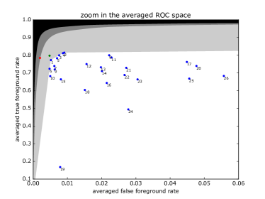
Figure 1: The $\overline{\textrm{ROC}}$ space with the $26$ BGS algorithms (${\color[rgb]{0.04296875,0.140625,0.984375}\bullet}$), previous state-of-the-art combination results (${\color[rgb]{0.05859375,0.49609375,0.0703125}\bullet}$ for IUTIS-5 [7] and $\bullet$ for CNN-SFC [8]), and the sets of achievable performances with the strategies Random Choice ($\square$ for $n=26$, see Section 3.1) and All Combinations ($\square\cup{\color[rgb]{0.80078125,0.80078125,0.80078125}\blacksquare}$ for $n\leq 9$, and $\square\cup{\color[rgb]{0.80078125,0.80078125,0.80078125}\blacksquare}\cup{\color[rgb]{0.5,0.5,0.5}\blacksquare}$ for $n=26$, see Section 3.2).

We analyze the sets of achievable performances for the $6$ combination strategies and $26$ unsupervised BGS algorithms.

A huge potential for the pixelwise combinations.

Figure 1 shows individual performances and sets of achievable performances in $\overline{\textrm{ROC}}$. According to it, the margin for improving the BGS performance is huge. Some pixelwise combinations of outputs (All Combinations) can drastically outperform all the individual BGS algorithms listed in Table 1. They can also largely outperform the simple Random Choice strategy. Moreover, there exist achievable performances that are closer to the oracle (upper left corner) than those of the non-pixelwise combinations IUTIS-5 and CNN-SFC.

There are efficient combination strategies.

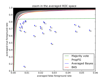
Figure 2: The $\overline{\textrm{ROC}}$ space with the convex hulls of performances achievable by combining $n\leq 9$ algorithms with four deterministic strategies (colored curves, see Section 3.3).

A combination strategy is efficient when (1) it produces a tractable amount of combinations, and (2) most of the performances achievable with All Combinations are also achievable by randomly choosing between some of the combinations produced by that strategy. Table 2 confirms that the amounts of combinations produced by our four deterministic strategies are all largely inferior to $2^{2^{n}}$. Figure 2 facilitates the comparison between the convex hulls of their performance point clouds and the achievable zone with All Combinations, in $\overline{\textrm{ROC}}$. We see that Prop. FG, Averaged Bayes, and BKS are efficient (and have approximately the same convex hulls), but not the classical Majority Vote. Little has to be gained from other pixelwise combination strategies (training decision trees or deep neural networks, adding some regularization to BKS, …) if the amount of combined algorithms is not increased.

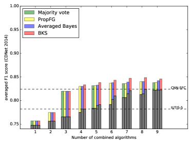
Figure 3: Best $\overline{\textrm{F}_{1}}$ scores for four deterministic combination strategies obtained with respect to the number $n=k,\,k\in\{1,\ldots,9\}$ of combined BGS algorithms. Gray bars indicate the results obtained with the top-$n$ algorithms (ranking of CDnet) instead of an optimized selection of $n$ algorithms.

	Combination strategy	Selection of BGS algorithms	$n$	Threshold $\tau$	$\overline{\textrm{F}_{1}}$ score
Previous works	IUTIS-5 [7]	SuBSENSE + FTSG + CwisarDH + Spectral360 + AMBER	$5$	None	$0.7821$
	CNN-SFC [8]	SuBSENSE + FTSG + CwisarDH	$3$	Unknown	$0.8243$
Ours	Majority Vote	PAWCS + WeSamBE + FTSG + CwisarDRP + MBS + CEFIC + MBSv0 + EFIC + GraphCutDiff	$9$	None	$0.8380$
	Prop. FG	PAWCS + WeSamBE + FTSG + CwisarDRP + MBS + CEFIC + MBSv0 + EFIC	$8$	$\nicefrac{{7}}{{16}}$	$0.8401$
	Averaged Bayes	PAWCS + WeSamBE + FTSG + CwisarDRP + MBS + CEFIC + MBSv0 + EFIC + GraphCutDiff	$9$	$0.2918$	$0.8421$
	BKS	PAWCS + FTSG + CwisarDRP + MBS + CEFIC + MBSv0 + EFIC + Euclidean	$8$	$0.2720$	$\mathbf{0.8487}$

Table 3: Summary of $\overline{\textrm{F}_{1}}$ scores including those of previous works (non-pixelwise combinations), and the maximum scores that are achievable with our four deterministic combination strategies by tuning the selection of algorithms and the threshold (pixelwise combinations). Note that our best score ($0.8487$) surpasses the one of CNN-SFC.

It is worth investigating combinations of BGS algorithms.

Figure 3 shows that the best $\overline{\textrm{F}_{1}}$ scores are, for $n>1$, significantly better than those obtained without combination ($n=1$). This suggests that looking for efficient combinations of existing BGS algorithms or developing new BGS algorithms complementary to the existing ones, even if not necessarily better, might be more profitable than searching for the best algorithm. Despite the fact that this conclusion was already drawn in [6], the BGS community continues to propose hundreds of new BGS algorithms every year, the best of which work barely better than the state of the art, without investigating the contribution of the proposed algorithms when combined with those already described in the literature.

How should we combine?

Figure 3 also helps in observing that our four deterministic strategies achieve the same maximal $\overline{\textrm{F}_{1}}$ score for $n\in\left\{2,3\right\}$. For $4\leq n\leq 9$, the ranking according to $\overline{\textrm{F}_{1}}$ is: $\emph{Majority Vote}\leq\emph{Prop. FG}\simeq\emph{Averaged Bayes}\leq\emph{BKS}$. Despite that, the improvement of Averaged Bayes and BKS performance is too small to balance their much larger amount of combinations to test in practice.

What should we combine?

For any given $n$, it might be tempting to combine the top-$n$ algorithms. In fact, Figure 3 shows that we can do much better by carefully cherry picking the combined algorithms among all the available ones (see colored bars vs. gray bars). Moreover, the difference in performance between a colored bar and the corresponding gray bar is, in most cases, greater than the difference in performance between adjacent gray bars. This suggests that knowing precisely what to combine is more important than knowing precisely how to combine. Poorly ranked algorithms can be useful when combined with others, even if they do not perform well alone. This is illustrated in Table 3, where we can observe that our best result are obtained by selecting algorithms in different zones of the leaderboard.

A new “state-of-the-art” $\textrm{F}_{1}$ score on CDnet 2014.

Our four deterministic strategies can outperform IUTIS-5 and CNN-SFC when the combined algorithms and the threshold $\tau$ are adequately chosen. As shown in Table 3, our results establish a new “state-of-the-art” $\textrm{F}_{1}$ score of $0.8487$ on CDnet 2014, against $0.8243$ for the previous one.

5 Conclusion

To push the performance in BGS, one can either develop new algorithms and publish their results on CDnet, or develop combinations based on the results already available on this platform. Our results show that such combinations have the potential to outperform the individual algorithms. This has resulted in six conclusions. Our findings were all made possible thanks to the availability of outputs on the CDnet platform, a choice that should be promoted for all challenges!

Acknowledgment.

This work was supported by the Service Public de Wallonie (SPW) Recherche, under Grant $\text{N}^{\text{o}}$. 2010235 – ARIAC by DigitalWallonia4.ai.

References

- [1] Y. Wang, P.-M. Jodoin, F. Porikli, J. Konrad, Y. Benezeth, and P. Ishwar, “CDnet 2014: An expanded change detection benchmark dataset,” in IEEE International Conference on Computer Vision and Pattern Recognition Workshops (CVPRW), Columbus, Ohio, USA, June 2014, pp. 393–400.
- [2] T. Bouwmans, “Traditional and recent approaches in background modeling for foreground detection: An overview,” Computer Science Review, vol. 11-12, pp. 31–66, May 2014.
- [3] T. Bouwmans, S. Javed, M. Sultana, and S. Jung, “Deep neural network concepts for background subtraction: A systematic review and comparative evaluation,” Neural Networks, vol. 117, pp. 8–66, September 2019.
- [4] B. Garcia-Garcia, T. Bouwmans, and A. J. Rosales Silva, “Background subtraction in real applications: Challenges, current models and future directions,” Computer Science Review, vol. 35, pp. 1–42, February 2020.
- [5] M. Mandal and S. Vipparthi, “An empirical review of deep learning frameworks for change detection: Model design, experimental frameworks, challenges and research needs,” IEEE Transactions on Intelligent Transportation Systems, vol. Early access, pp. 1–22, 2021.
- [6] P.-M. Jodoin, S. Piérard, Y. Wang, and M. Van Droogenbroeck, “Overview and benchmarking of motion detection methods,” in Background Modeling and Foreground Detection for Video Surveillance, chapter 24. Chapman and Hall/CRC, July 2014.
- [7] S. Bianco, G. Ciocca, and R. Schettini, “Combination of video change detection algorithms by genetic programming,” IEEE Transactions on Evolutionary Computation, vol. 21, no. 6, pp. 914–928, December 2017.
- [8] D. Zeng, M. Zhu, and A. Kuijper, “Combining background subtraction algorithms with convolutional neural network,” CoRR, vol. abs/1807.02080, 2018.
- [9] P.-L. St-Charles, G.-A. Bilodeau, and R. Bergevin, “Universal background subtraction using word consensus models,” IEEE Transactions on Image Processing, vol. 25, no. 10, pp. 4768–4781, October 2016.
- [10] P.-L. St-Charles, G.-A. Bilodeau, and R. Bergevin, “SuBSENSE: A universal change detection method with local adaptive sensitivity,” IEEE Transactions on Image Processing, vol. 24, no. 1, pp. 359–373, January 2015.
- [11] S. Jiang and X. Lu, “WeSamBE: A weight-sample-based method for background subtraction,” IEEE Transactions on Circuits and Systems for Video Technology, vol. 28, no. 9, pp. 2105–2115, September 2018.
- [12] Y. Chen, J. Wang, and H. Lu, “Learning sharable models for robust background subtraction,” in IEEE International Conference on Multimedia and Expo (ICME), Turin, Italy, June-July 2015, pp. 1–6.
- [13] R. Wang, F. Bunyak, G. Seetheraman, and K. Palaniappan, “Static and moving object detection using flux tensor with split Gaussian models,” in IEEE International Conference on Computer Vision and Pattern Recognition Workshops (CVPRW), Columbus, Ohio, USA, June 2014, pp. 414–418.
- [14] M. De Gregorio and M. Giordano, “WiSARD for change detection in video sequences,” in European Symposium on Artificial Neural Networks, Computational Intelligence and Machine Learning (ESANN), Bruges, Belgium, April 2017, pp. 453–458.
- [15] H. Sajid and S.-C. Cheung, “Universal multimode background subtraction,” IEEE Transactions on Image Processing, vol. 26, no. 7, pp. 3249–3260, July 2017.
- [16] G. Allebosch, D. Van Hamme, F. Deboeverie, P. Veelaert, and W. Philips, “C-EFIC: color and edge based foreground background segmentation with interior classification,” in Computer Vision, Imaging and Computer Graphics Theory and Applications (VISIGRAPP), Berlin Germany, March 2015, pp. 433–454.
- [17] H. Sajid and S.-C. Cheung, “Background subtraction for static & moving camera,” in IEEE International Conference on Image Processing (ICIP), Quebec, Canada, September 2015, pp. 4530–4534.
- [18] M. De Gregorio and M. Giordano, “Change detection with weightless neural networks,” in IEEE International Conference on Computer Vision and Pattern Recognition Workshops (CVPRW), Columbus, Ohio, USA, June 2014, pp. 409–413.
- [19] G. Allebosch, F. Deboeverie, P. Veelart, and W. Philips, “EFIC: Edge based foreground background segmentation and interior classification for dynamic camera viewpoints,” in Advanced Concepts for Intelligent Vision Systems (ACIVS). October 2015, vol. 9386 of Lecture Notes in Computer Science, pp. 130–141, Springer.
- [20] M. Sedky, M. Moniri, and C. Chibelushi, “Spectral 360: A physics-based technique for change detection,” in IEEE International Conference on Computer Vision and Pattern Recognition Workshops (CVPRW), Columbus, Ohio, USA, June 2014, pp. 399–402.
- [21] I. Martins, P. Carvalho, L. Corte-Real, and J. Alba-Castro, “BMOG: Boosted gaussian mixture model with controlled complexity,” in Iberian Conference on Pattern Recognition and Image Analysis (ibPRIA). June 2017, vol. 10255 of Lecture Notes in Computer Science, pp. 50–57, Springer.
- [22] B. Wang and P. Dudek, “A fast self-tuning background subtraction algorithm,” in IEEE International Conference on Computer Vision and Pattern Recognition Workshops (CVPRW), Columbus, Ohio, USA, June 2014, pp. 395–399.
- [23] G. Ramírez-Alonso and M. Chacón-Murguía, “Auto-adaptive parallel som architecture with a modular analysis for dynamic object segmentation in videos,” Neurocomputing, vol. 175, pp. 990–1000, January 2016.
- [24] A. Miron and A. Badii, “Change detection based on graph cuts,” in IEEE International Conference on Systems, Signals and Image Processing (IWSSIP), London, England, UK, September 2015, pp. 273–276.
- [25] L. Maddalena and A. Petrosino, “The SOBS algorithm: what are the limits?,” in IEEE International Conference on Computer Vision and Pattern Recognition Workshops (CVPRW), Providence, Rhode Island, USA, June 2012, pp. 21–26.
- [26] S. Varadarajan, P. Miller, and H. Zhou, “Spatial mixture of Gaussians for dynamic background modelling,” in IEEE International Conference on Advanced Video and Signal Based Surveillance, Krakow, Poland, August 2013, pp. 63–68.
- [27] Y. Benezeth, P.-M. Jodoin, B. Emile, H. Laurent, and C. Rosenberger, “Comparative study of background subtraction algorithms,” Journal of Electronic Imaging, vol. 19, no. 3, pp. 1–12, 2010.
- [28] A. Elgammal, D. Harwood, and L. Davis, “Non-parametric model for background subtraction,” in European Conference on Computer Vision (ECCV). June 2000, vol. 1843 of Lecture Notes in Computer Science, pp. 751–767, Springer.
- [29] D. Liang, S. Kaneko, M. Hashimoto, K. Iwata, and X. Zhao, “Co-occurrence probability-based pixel pairs background model for robust object detection in dynamic scenes,” Pattern Recognition, vol. 48, no. 4, pp. 1374–1390, April 2015.
- [30] C. Stauffer and E. Grimson, “Adaptive background mixture models for real-time tracking,” in IEEE International Conference on Computer Vision and Pattern Recognition (CVPR), Fort Collins, Colorado, USA, June 1999, vol. 2, pp. 246–252.
- [31] Z. Zivkovic, “Improved adaptive Gaussian mixture model for background subtraction,” in IEEE International Conference on Pattern Recognition (ICPR), Cambridge, UK, August 2004, vol. 2, pp. 28–31.
- [32] K. Sehairi, F. Chouireb, and J. Meunier, “Comparative study of motion detection methods for video surveillance systems,” Journal of Electronic Imaging, vol. 26, no. 2, pp. 1–29, April 2017.
- [33] X. Lu, “A multiscale spatio-temporal background model for motion detection,” in IEEE International Conference on Image Processing (ICIP), Paris, France, October 2014, pp. 3268–3271.
- [34] Y. Huang and C. Suen, “A method of combining multiple experts for the recognition of unconstrained handwritten numerals,” IEEE Transactions on Pattern Analysis and Machine Intelligence, vol. 17, no. 1, pp. 90–94, January 1995.
- [35] L. Kuncheva, C. Whitaker, C. Shipp, and R. Duin, “Limits on the majority vote accuracy in classifier fusion,” Pattern Analysis & Applications, vol. 6, no. 1, pp. 22–31, April 2003.
- [36] S. Piérard and M. Van Droogenbroeck, “Summarizing the performances of a background subtraction algorithm measured on several videos,” in IEEE International Conference on Image Processing (ICIP), Abu Dhabi, United Arab Emirates, October 2020, pp. 3234–3238.
- [37] T. Fawcett, “An introduction to ROC analysis,” Pattern Recognition Letters, vol. 27, no. 8, pp. 861–874, June 2006.