Efficient Query Re-optimization with Judicious Subquery Selections

Abstract.

Query re-optimization is an adaptive query processing technique that re-invokes the optimizer at certain points in query execution. The goal is to dynamically correct the cardinality estimation errors using the statistics collected at runtime to adjust the query plan to improve the overall performance. We identify a key weakness in existing re-optimization algorithms: their subquery division and re-optimization trigger strategies rely heavily on the optimizer’s initial plan, which can be far away from optimal. We, therefore, propose QuerySplit, a novel re-optimization algorithm that skips the potentially misleading global plan and instead generates subqueries directly from the logical plan as the basic re-optimization units. By developing a cost function that prioritizes the execution of less “damaging” subqueries, QuerySplit successfully postpones (sometimes avoids) the execution of complex large joins to maximize their probability of having smaller input sizes. We implemented QuerySplit in PostgreSQL and compared our solution against four state-of-the-art re-optimization algorithms using the Join Order Benchmark. Our experiments show that QuerySplit reduces the benchmark execution time by $35\%$ compared to the second-best alternative. The performance gap between QuerySplit and an optimal optimizer is within $4\%$.

1. Introduction

Given a query, a cost-based optimizer in a relational database management system (DBMS) enumerates a subset of valid plans through dynamic programming and computes the cost for each plan by feeding the estimated cardinalities of the intermediate results to the cost model. If such estimations are way off, no matter how precise the cost model is, the optimizer is likely to choose a sub-optimal plan, thus slowing down the query (Leis et al., 2015). Unfortunately, it is difficult to get accurate cardinality estimations (CE) consistently, especially for joins because columns are often correlated in real-world data sets (Wu et al., 2016; Perron et al., 2019). Researchers have proposed new approaches beyond conventional histograms, including multidimensional histogram (Gunopulos et al., 2005), sketch (Rusu and Dobra, 2008; Cai et al., 2019), sampling (Leis et al., 2017; Wu et al., 2016) and machine learning (Wang et al., 2020) to improve on the CE accuracy. None of them, however, is robust enough to be able to declare victory in solving the problem (Leis et al., 2015, 2018; Perron et al., 2019).

The intrinsic difficulty of cardinality estimation calls for alternative approaches to query optimizations. One of such is re-optimization (Kabra and DeWitt, 1998; Markl et al., 2004; Kaftan et al., 2018; Perron et al., 2019; Neumann and Galindo-Legaria, 2013). The idea is straight-forward: if the optimizer cannot make accurate predictions of the cardinalities upfront, we will have to correct its mistakes dynamically at runtime. Therefore, the process of re-optimization is an interleaving of query execution and query optimization: it executes the query partially, obtains some true cardinalities and runtime statistics, and then invokes the optimizer again, hoping to improve the efficiency of the remaining plan. The recent investigation by Perron et al. shows that even a basic re-optimization strategy could remedy a significant portion of the performance losses caused by cardinality mis-estimations (Perron et al., 2019).

The key problem of designing a re-optimization strategy is to decide (1) which subquery to execute next and (2) when to materialize the intermediate results and re-invoke the optimizer. Existing solutions rely heavily on the optimizer’s initial plan (Kabra and DeWitt, 1998; Markl et al., 2004; Perron et al., 2019; Neumann and Galindo-Legaria, 2013). They repeatedly extract subtrees from the complete plan to execute and then use the results to refine the remaining parts. The initial plan, however, can be far away from optimal because of inaccurate cardinality estimations. In this case, the DBMS is likely to choose the “wrong” subplan (e.g., costly itself or generate large results) to execute first, and such a mistake is often unrecoverable by subsequent re-optimization steps.

Meanwhile, these solutions are “reactive” in terms of when to trigger re-optimization, i.e., the re-optimization frequency depends heavily on the initial physical plan. For example, mid-query re-optimization by Kabra et al. only materializes results at pipeline breakers (e.g., a sort operation) (Kabra and DeWitt, 1998). Consequently, for a left-deep join tree where each join is a nested-loop join, re-optimization is never triggered. On the contrary, Pop aggressively materializes the output at every nested-loop join, causing a large performance and space overhead because of re-optimization (Markl et al., 2004).

In this paper, we propose a novel re-optimization algorithm, called QuerySplit, to address the above issues. The key idea is to skip the potentially misleading global plans and instead extract subqueries directly from the logical plan as the basic units for re-optimization. Join operators in the logical plan are grouped into subqueries according to heuristics developed from the primary-foreign-key relationships to bound/minimize the output sizes of intermediate results.

Such a “query split” algorithm is more robust to balance the gains and costs of re-optimization than those operating on the physical plan. QuerySplit then adopts a greedy algorithm to select a subquery with the smallest cost and output cardinality to execute first. The intuition is that the performance of a complex query is often determined by a few large joins (e.g., fact-fact table join). By executing “simpler” (or “less-damaging”) subqueries first and re-optimizing the rest, we increase the probability of delaying the execution of those large joins and thus approaching an optimal plan. Notice that the re-optimization points are purely determined by the logical plan. The optimizer is only invoked for the subqueries to get/update their costs and output cardinalities at each iteration, and the subqueries are usually simple enough for existing optimizers to generate reasonably good plans quickly.

We implemented QuerySplit in PostgreSQL and compared our algorithm against the state-of-the-art re-optimization solutions (Kabra and DeWitt, 1998; Markl et al., 2004; Neumann and Galindo-Legaria, 2013; Perron et al., 2019), robust query processing techniques (Hertzschuch et al., 2021; Cai et al., 2019; Wolf et al., 2018a, b), and learned cardinality estimation algorithms (Yang et al., 2020; Hilprecht et al., 2019; Kipf et al., 2018) on the Join Order Benchmark (JOB) (Leis et al., 2015) (as well as TPC-H (TPC, 2022b) and Decision Support Benchmark (DSB) (Ding et al., 2021)). Our experiments show that QuerySplit reduces the JOB execution time by $35\%$ as opposed to the second-best alternative algorithm. Moreover, compared to an optimal optimizer (i.e., an optimizer fed by the true cardinality of each operator), QuerySplit slows down the benchmark execution by less than $4\%$.

The contributions of this paper are as follows. First, we identified that relying on the sub-optimal initial plan is a key weakness of existing re-optimization strategies. Second, we proposed the QuerySplit algorithm that extracted subqueries directly from the logical plan based on the primary-foreign-key relationships to achieve a robust re-optimization efficiency. Finally, we integrated QuerySplit into PostgreSQL and demonstrated the superiority of our algorithm by comparing it to state-of-the-art solutions.

2. Background & Motivation

2.1. Cardinality Estimation

Cardinality estimation refers to the process of estimating the number of rows generated by each operator at query optimization. It is used as an input parameter to the optimizer’s cost model. Improved cardinality estimation enables more accurate cost estimation, thus helping the optimizer select an efficient plan. Most DBMSs maintain table/column-level statistics such as histograms and the number of distinct values, from which they derive the selectivity of basic single-column predicates. The more challenging tasks are to estimate the selectivity of conjunctive predicates involving multiple columns and to estimate the join cardinality. Because it is too costly to maintain a relatively complete set of multi-column statistics, the optimizer has to make assumptions about the correlation between columns in these cases.

Most widely-used DBMSs such as PostgreSQL and MySQL assume independent data distributions between columns (Leis et al., 2015; MySQL, 2020). It is probably one of the best strategies an optimizer could apply given the lack of statistics. In reality, however, highly correlated columns are common, and this approach is likely to deliver underestimated cardinalities (Leis et al., 2015). Although the accuracy of cardinality estimation for complex queries can be improved through sampling (Leis et al., 2017; Wu et al., 2016) and machine learning techniques (Wang et al., 2020), none of the approaches is robust enough, and their intrinsic overhead is hardly justified in real-world database applications (Perron et al., 2019). What makes it worse is error propagation. For an N-way natural join, for example, the cardinality estimation error at each join step could grow exponentially with N (Ioannidis and Christodoulakis, 1991). This theoretical result matches what we have observed in practice.

2.2. Re-optimization

Query re-optimization is a technique of adaptive query processing (Babu and Bizarro, 2005; Deshpande et al., 2007) where the optimizer is (re)invoked at execution time to correct potential bad plans. Specifically, the optimizer selects a few operations in the physical plan to materialize the intermediate results. It then compares the true cardinality (i.e., statistics from the actual intermediate results) against the previously estimated value. If those values differ too much, the optimizer would re-plan the remaining part of the query using the true cardinality. Although re-optimization itself brings overheads, the revised plan is almost guaranteed to be at least as good as the original one. Re-optimization, therefore, is a process of interleaving the execution of the query engine and the optimizer, as shown in Figure 1.

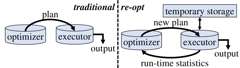
Figure 1. Structure difference between traditional query processing and re-optimization

Existing re-optimization algorithms (Kabra and DeWitt, 1998; Markl et al., 2004; Perron et al., 2019; Neumann and Galindo-Legaria, 2013) operate directly on global physical plans. They choose a subtree from the plan obtained from the previous re-optimization cycle and execute that subplan to decide whether further re-optimization is needed. Such a strategy of “selecting a partial query to execute” can be problematic if the referencing global plan deviates largely from an optimal one. And once an undesirable subplan (typically involving large tables but with an underestimated cardinality) is chosen, the damage often propagates through later re-optimization iterations.

Figure 2 shows an example to illustrate such an unrecoverable subplan execution. The query is a 5-way join extracted from the JOB benchmark. There is an index built for each join column. As shown in Figure 2(a), the optimal plan joins table n and ci first and uses the results to probe table t in an index nested-loop join (denoted as NL in the figure). The actual initial plan (Figure 2(b)), however, underestimates the cardinality of k $\Join$ mk and thus chooses to execute this subplan first. We use S₁ to denote the intermediate result of k $\Join$ mk. Once we discover that S₁ is much larger than the prior estimation, we trigger the optimizer to re-plan the rest of the query. However, the best the optimizer can do at this point is shown in Figure 2(c). Because the large temporary table S₁ does not have an index, the DBMS must perform a hash join (highlighted in bold red) for the last step, which could be orders of magnitude slower than probing the existing indexes of the two base tables.

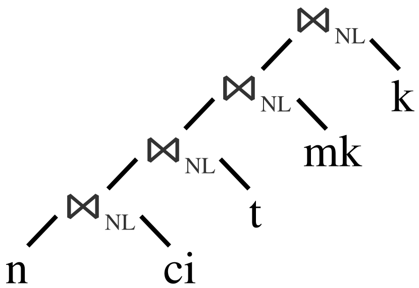
(a) Optimal plan

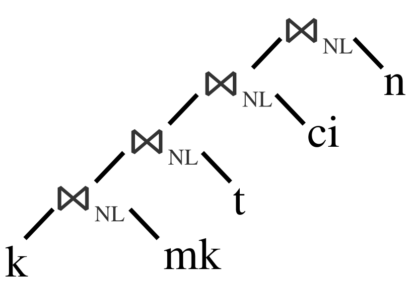
(b) Initial plan

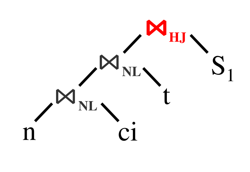
(c) Re-Optimized plan after the first join

Figure 2. The example of how a bad global plan influence re-optimization

To show how much an initial global plan can deviate from optimal, we investigate the query plans in the Join Order Benchmark using the optimizer from PostgreSQL. We define the similarity score of two plans as the number of leaf nodes included in their largest common subtree. For example, as shown in Figure 3, if the first joins of the two plans differ completely, they have a similarity score of 0 (Figure 3(a)); if the probe side scans the same table (but joins a different one), the similarity of the plans is 1 (Figure 3(b)); similarity = 2 means that the plans differ after the first join (Figure 3(c)). In Table 1, we demonstrate how often initial global plans diverge from the optimal ones early in the execution. We observe that more than half of the JOB queries have initial plans whose optimality does not “survive” after one join, among which a quarter of the plans even made mistakes on the first join.

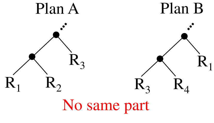
(a) Similarity = 0

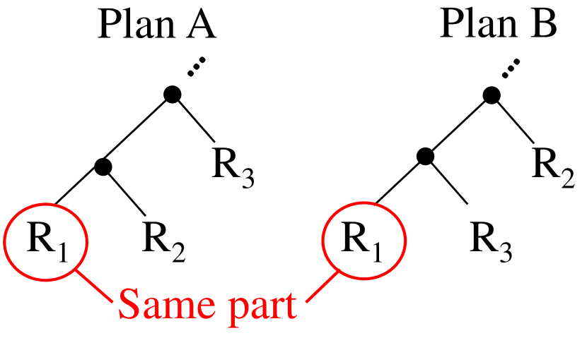
(b) Similarity = 1

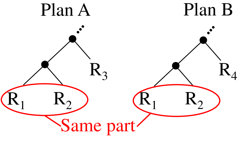
(c) Similarity = 2

Figure 3. The example of different similarity

Table 1. The ratio of queries whose global plans deviate from the optimal plan with different degrees

Similarity	0	1	2	¿ 2
Ratio	13%	12%	32%	43%

The second problem of existing algorithms is that the re-optimization decision is made reactively according to the types of physical plan nodes. Such a heuristic-based approach often leads to extreme re-optimization frequencies. If the system triggers re-optimization only at pipeline breakers, it never gets a chance to change the ordering of the nested-loop joins in a left-deep plan. On the other hand, if the system invokes re-optimization at every join, the overhead of materializing intermediate results might be intimidating: it essentially converts the execution from the Volcano model to the fully-materialized one.

2.3. A Proactive Strategy

As shown in Section 2.2, a suboptimal global plan can cause irrecoverable damages to the effectiveness of existing re-optimization algorithms. We, therefore, argue that a better strategy is to examine the query’s logical plan and decide proactively when to materialize results (and re-invoke the optimizer) before execution. We call this scheme QuerySplit. Specifically, we divide the logical plan into subqueries based on the primary-foreign-key relationships and optimize them separately. Because each subquery is relatively simple, it is less likely that the optimizer would make serious mistakes as in a global plan. We then choose one of the subqueries to run and materialize its output. Once the execution is finished, we use the updated statistics (e.g., output size) to re-optimize the remaining relevant subqueries. This process continues until no subquery is left to be executed. The execution order is determined by a “ranking” function (detailed in Section 4.2) where subqueries with small costs and output sizes are prioritized.

Figure 4 shows an example of a 5-way join re-optimized using QuerySplit. We first split the query into three subqueries and optimize them separately: S₁=R₂ $\Join$ R₃, S₂=R₃ $\Join$ R₄ $\Join$ R₅, and S₃=R₁ $\Join$ R₂. We then choose S₁ to execute and materialize its output as T₁. Using the statistics of T₁, we trigger re-optimization on the remaining subqueries S₂=T₁ $\Join$ R₄ $\Join$ R₅ and S₃=R₁ $\Join$ T₁ (Figure 4(c)). S₂ is selected to run next. The result is materialized in T₂, whose statistics is used to re-optimize the final subquery S₃=R₁ $\Join$ T₂.

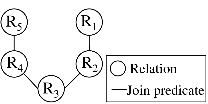
(a) Logical Plan

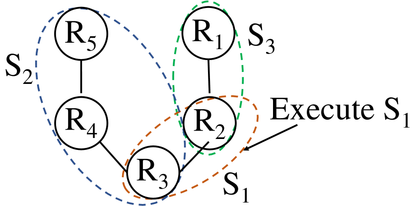
(b) Subqueries S₁, S₂, and S₃

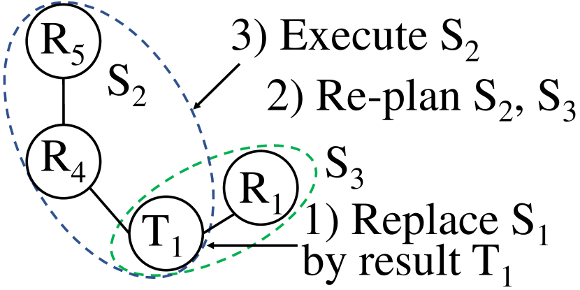
(c) Re-optimizing S₂ and S₃

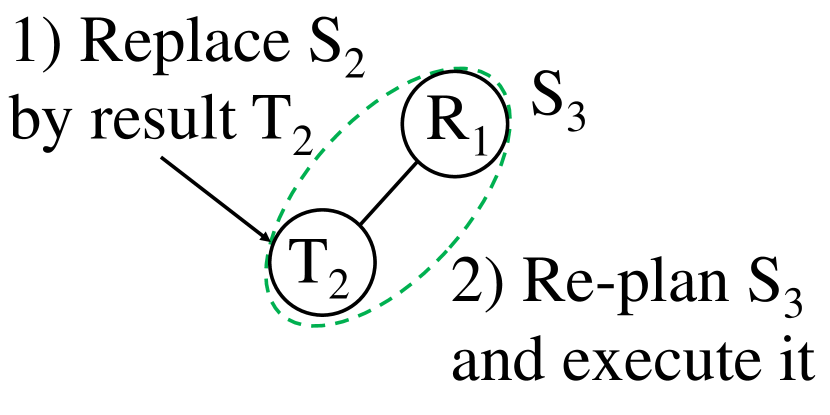
(d) Re-optimizing S₃

Figure 4. QuerySplit example

Compared to traditional re-optimization algorithms, QuerySplit is more robust at avoiding suboptimal plans, and has more control over the re-optimization cost. First, QuerySplit does not depend on global physical plans. Because the difficulty of the optimization task grows exponentially as the number of joins increases, the optimizer is likely to make mistakes when planning a complex query by entirety. As discussed in Section 2.2, “early mistakes” are common and they cannot be recovered through re-optimization. In QuerySplit, on the other hand, the optimizer only deals with much simpler subqueries, and the probability of generating bad plans is reduced dramatically.

Second, QuerySplit has predictable re-optimization overhead because it determines where to re-invoke the optimizer before executing the query. The overhead is also adjustable by modifying the subquery granularity. In this way, QuerySplit avoids undesirable re-optimization frequencies caused by various physical plan shapes, as described in Section 2.2. The trade-off, though, is that QuerySplit might miss certain optimization opportunities that are only recognizable when examining the query as a whole. QuerySplit could be “myopic” because the optimizer only operates at the subquery level. Our detailed evaluation (Sections 6.3 and 6.5), however, demonstrate that such a trade-off is modest and is outweighed by the aforementioned benefits.

The rest of the paper is organized as follows. Section 3 provides an overview of QuerySplit with correctness proof. Section 4 discusses two critical policies that could largely determine the efficiency of our algorithm. Section 5 briefly describes the integration of QuerySplit into PostgreSQL. An evaluation of QuerySplit along with detailed case studies is presented in Section 6 followed by the related work in Section 7.

3. QuerySplit

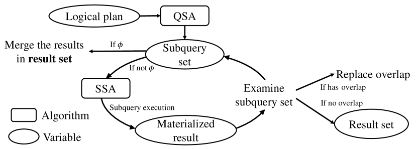
Figure 5. The workflow of QuerySplit

In this section, we present an overview of the QuerySplit algorithm followed by a proof of correctness. Algorithm details and implementation are further discussed in Section 4.

3.1. Algorithm Overview

As shown in Figure 5, QuerySplit takes in a query’s logical plan and runs the Query Splitting Algorithm (QSA) against it. For simplicity, we restrict the input to be select-projection-join (SPJ) queries only (i.e., queries involving only select, projection, and join operators). Algorithm extension to support non-SPJ queries is discussed in Section 3.3. The goal of QSA is to generate a set of subqueries where a serial execution of the subqueries would have the same result as executing the original query. We discuss the requirements of such a valid subquery set in Section 3.2.

With a valid subquery set, QuerySplit proceeds to enter a loop. At each loop iteration, QuerySplit picks a subquery from the current set to execute according to the Subquery Selection Algorithm (SSA). Although SSA does not affect correctness, it has a significant impact on the efficiency of the entire QuerySplit algorithm. We discuss different subquery ranking strategies in detail in Section 4.2. The selected subquery is then removed from the set, and the execution results as well as the associated statistics are materialized.

Next, QuerySplit examines each of the remaining subqueries in the set: if it overlaps with the just-executed subquery (i.e., they have shared relations), the shared relations are replaced with the corresponding materialized results. If it turns out that the just-executed subquery does not overlap with any of the subqueries in the set, its execution results are pushed to the result set. The loop continues until the subquery set becomes empty. Finally, QuerySplit merges the results (through Cartesian product) if there are multiple items in the result set.

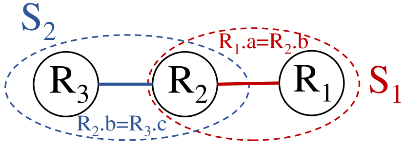
(a) Original subquery set

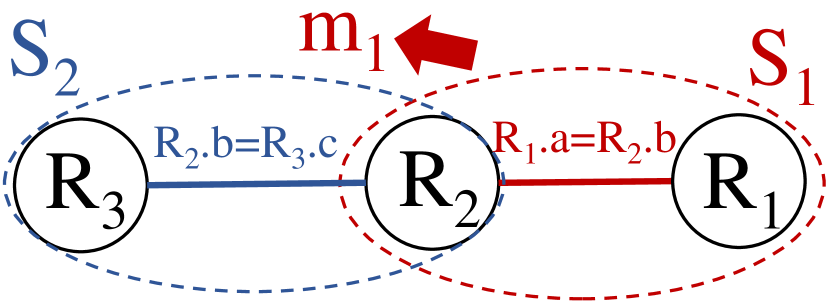
(b) Execute S₁

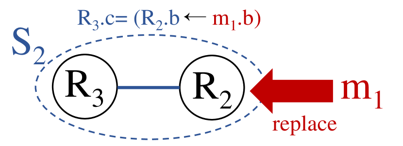
(c) Modify S₂

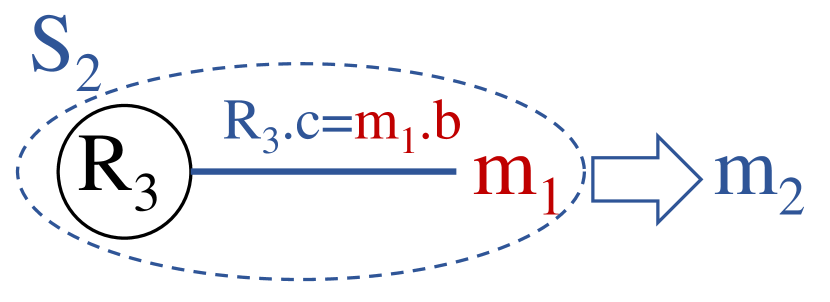
(d) Execute S₂

Figure 6. An example of how QuerySplit works

Figure 6 shows an example. The original query is $R1\Join_{R1.a=R2.b}R2\Join_{R2.b=R3.c}R3$, where $R1.a$ denotes attribute $a$ from relation $R1$. After running the QSA, we obtain two subqueries in the set: $S1=R1\Join_{R1.a=R2.b}R2$ and $S2=R2\Join_{R2.b=R3.c}R3$. Suppose the SSA selects $S1$ to execute first, and the materialized result is denoted by $m1$. We next examine the remaining subquery $S2$. Because $S2$ and $S1$ share the common relation $R2$, we substitute $m1$ for $R2$ and rewrite $S2$ as $m1\Join_{m1.b=R3.c}R3$. We then enter the next iteration and execute $S2$. Because there is no more subquery in the set, we push the execution result $m2$ to the result set and complete the algorithm.

Notice that the projection operators can be added to the subqueries following the general projection push-down rules. We omit projections in the following discussions for presentation clarity.

3.2. Correctness

As indicated above, the correctness of QuerySplit depends on the output of QSA (i.e., the subquery set). In this subsection, we define the required properties of the subquery set and prove that the QuerySplit algorithm is correct given a valid subquery set.

Given a set of relations R and a set of predicates P over R, we define the normal form of an SPJ query as

$$q(\textbf{{R}},\textbf{{P}})=(\sigma_{\textbf{{P}}}(r_{1}\times r_{2}\times...\times r_{m})),r_{i}\in\textbf{{R}}$$

A query $q^{\prime}(\textbf{{R}}^{\prime},\textbf{{P}}^{\prime})$ is said to be a subquery of $q(\textbf{{R}},\textbf{{P}})$ if $\textbf{{R}}^{\prime}\subseteq\textbf{{R}}$ and $\textbf{{P}}^{\prime}\subseteq\textbf{{P}}$. A Query Splitting Algorithm (QSA) takes a query $q$ as input and produces a set of subqueries of $q$. QuerySplit then operates on this subquery set, as described in Section 3.1. Intuitively, in order for QuerySplit to produce the same result as the original query, the subquery set generated by QSA must “cover” all the relations and predicates in the original query. More formally,

Definition 1.

Given an SPJ query $q(\textbf{{R}},\textbf{{P}})$, let $\textbf{{Q}}=\{q_{1}(\textbf{{R}}_{1},\textbf{{P}}_{1})$, …, $q_{n}(\textbf{{R}}_{n},\textbf{{P}}_{n})\}$ be a set of subqueries of q. Q is said to cover $q$ (denoted as $\textbf{{Q}}\rightharpoonup_{c}q$) if the following holds:
(1) $\cup_{i=1}^{n}\textbf{{R}}_{i}=\textbf{{R}}$
(2) $\cup_{i=1}^{n}\textbf{{P}}_{i}$ logically implies P.

The above definition guarantees that each base relation $r_{i}$ in R and each predicate $p_{i}$ in P must appear at least once in the subquery set Q. Notice that the definition allows the same $r_{i}$ or $p_{i}$ to be included in multiple subqueries. This does not affect the correctness of the QuerySplit algorithm because the duplicates will be removed during the (materialized) result substitution step. In fact, the “coverness” property is sufficient to prove the correctness of the entire QuerySplit algorithm.

Theorem 0 (1).

Let $q(\textbf{{R}},\textbf{{P}})$ be an SPJ query, Q be a set of subqueries of $q$. QuerySplit produces the same output as $q$ if $\textbf{{Q}}\rightharpoonup_{c}q$.

Proof sketch: We prove the theorem by induction. For the base case, if there is only one query $q^{\prime}$ in Q, and $\textbf{{Q}}\rightharpoonup_{c}q$, then $q^{\prime}$ and $q$ are equivalent queries. Suppose the statement is true for $\lvert\textbf{{Q}}\rvert=n-1$, we want to prove that it also holds for $\lvert\textbf{{Q}}\rvert=n$. Let $\textbf{{Q}}=\{q_{1},q_{2},...,q_{n}\}$. Without loosing generality, suppose the first query executed by QuerySplit is $q_{1}$, and the remaining set is $\textbf{{Q'}}=\{q_{2},...,q_{n}\}$. If $q_{1}$ overlaps (i.e., with at least one shared relation) with a query $q_{i}$ in Q’, we can prove that substituting the materialized view of $q_{1}$ into $q_{i}$ does not change the overall query result. Then, the remaining subquery set (after the substitution) $\textbf{{Q''}}=\{q_{2},...,q^{\prime}_{i},...,q_{n}\}$ falls back to the induction hypothesis. On the other hand, if $q_{1}$ does not overlap with any of the queries in Q’, then executing this “isolated” subquery first and pushing its result to the final buffer does not affect the correctness of the original query. Again, after executing $q_{1}$, the remaining subquery set Q’ falls back to the induction hypothesis. A detailed proof can be found in Proof.

3.3. Extending to Non-SPJ Queries

The focus of the QuerySplit algorithm is on optimizing the join ordering of SPJ queries. In this subsection, we briefly discuss how to extend QuerySplit to be compatible with queries containing Non-SPJ operators.

First of all, we do not distinguish between the join types when running the QSA. After getting the subquery set, we perform an extra check for each subquery containing “special” joins (i.e., outer join, semi-join, and anti-join) to determine whether executing it in the current iteration would violate any ordering constraints. If a violation is detected, the subquery is temporarily removed from the candidate set for this iteration. If the candidate set becomes empty after the check, the execution falls back to follow a global physical plan.

Besides special joins, a majority of the Non-SPJ optimizations (e.g., subquery flattening/merging and outer join simplification) are performed at the rule-based transformation stage (Chaudhuri, 1998; MySQL, 2020; Documentation, 2021; Oracle, 2021). These optimizations happen before the QuerySplit algorithm, and their results (i.e., the transformed plan) are consumed by QuerySplit at the cost-based enumeration stage in the following way. Given a Non-SPJ operator (e.g., aggregation, semi join) $\phi$ whose inputs are generated by a set of SPJ subqueries $q_{1},q_{2},...,q_{n}$, we apply the QuerySplit algorithm to each of the subqueries and feed their results to $\phi$. Unlike the subquery execution within QuerySplit where the result must be materialized for re-optimization, the data transfer between $\phi$ and the $q_{i}$’s can be pipelined.

For a query plan that contains multiple Non-SPJ operators, we segment the plan tree according to these operators and execute them from the bottom up After completing each Non-SPJ operator, we materialize its result and treat it as a base relation in the subsequent QuerySplit invocations.

Figure 7 shows an example. On the left, there is a query plan containing two Non-SPJ operators: a Union and an Avg aggregation. We first divide the plan tree based on these two operators so that they become the roots of their own subtrees. For each of the subtree, we execute the SPJ part of the plan first. In the Avg subtree, for example, the subquery $R_{3}\Join R_{4}\Join R_{5}$ is first executed through QuerySplit, and the result is used as an input to the Avg operator. We then materialize the output of Avg and Union as relation $T_{1}$ and $T_{2}$, and use those to replace the corresponding subtrees in the root plan. Finally, we invoke QuerySplit again on the root plan to obtain the final result.

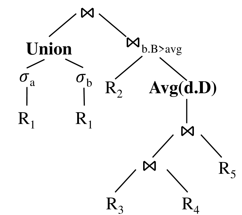
(a) Non-SPJ query

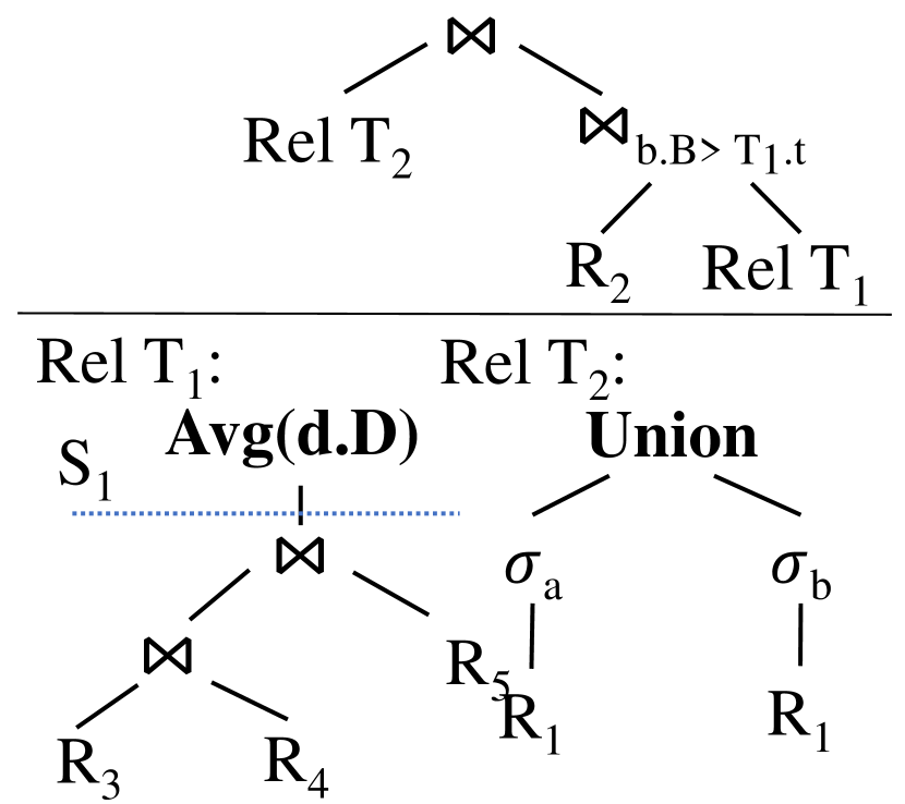
(b) New SPJ query

Figure 7. How to deal with non-SPJ query

Notice that a potential limitation of adopting the above Non-SPJ extension of QuerySplit is that it might miss a few global optimization opportunities such as group-by pushdown during the cost-based enumeration stage. Our evaluation on TPC-H (TPC, 2022b) and DSB (Ding et al., 2021) (an extension to TPC-DS (TPC, 2022a)) in Section 6 shows that such a negative impact is limited and is often outweighed by the benefit of a more optimized join ordering. A deeper integration of Non-SPJ operators into QuerySplit is beyond the scope of this paper, and we leave it as future work.

4. Subquery Creation & Selection Policies

In Section 3, we mainly focused on the correctness of the QuerySplit algorithm. To fully exploit QuerySplit’s ability to deliver good query performance, we discuss two critical policies in this section: (1) how to pick a subquery set from a (exponentially) large number of valid choices, and (2) how to select a subquery from an existing set at each QuerySplit iteration.

4.1. Generating a Subquery Set

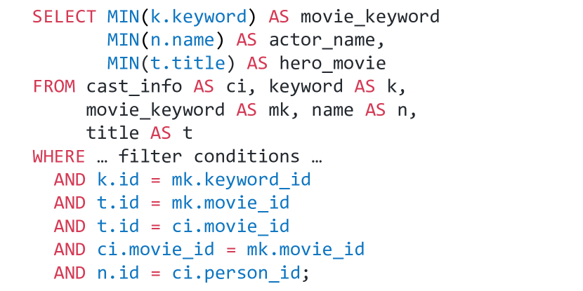
(a) Original SQL

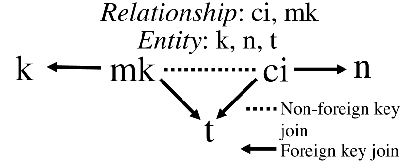
(b) Join schema

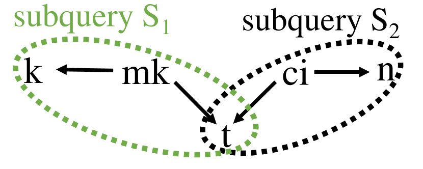
(c) Directed join graph

Figure 8. Join graph split by RelationshipCenter

As described in Section 3.2, a subquery set Q output by the Query Splitting Algorithm (QSA) is valid if it “covers” the original query $q$. The number of the candidate sets, however, grows exponentially with the complexity of $q$ (e.g., the number relations in $q$). The goal of the QSA is to perform an efficient search in the candidate space and produce a subquery set that best serves the overall QuerySplit algorithm.

Intuitively, we prefer subqueries that return small results. There are two potential advantages. First, the cost of materializing the output of such a subquery is small in each QuerySplit iteration. Second, because the materialized result will become a new base relation to participate in subsequent executions, having a smaller size is beneficial to improving the performance of succeeding subqueries.

We, therefore, propose a subquery generation strategy, called the FK-Center strategy (i.e., Foreign-Key-Center). FK-Center leverages the concept of non-expanding operators proposed by Hertzschuch et al. (Hertzschuch et al., 2021). A non-expanding operator is defined as an operator that has an output size smaller than or equal to its input size. The FK-Center strategy is based on the non-expanding property of the primary-foreign-key joins. Given a query, we define FK-relation as a relation that has at least one foreign-key reference to another relation and PK-relation as a relation whose primary key is referenced by other relations.

The RCenter strategy is based on the non-expanding property of the primary-foreign-key joins. Many relational database schemas follow the classic entity-relationship design (Chen, 1976) (i.e., the star schema) where a “relationship” relation (or the “fact” table) is at the center containing foreign keys referring to the surrounding “entity” relations (or “dimension” tables). Therefore, given a query, we define R-relation as a relation that has at least one foreign-key reference to another relation and E-relation as a relation whose primary key is referenced by other relations.

We then construct a directed join graph for the query where each vertex represents a relation and each edge represents a join predicate (single table predicates are associated with the vertices). For each edge, its direction is from an R-relation to an E-relation. If the join happens between two relations with the same type, the edge is bidirectional. Redundant join predicates (e.g., those form cycles in the join graph) are deleted with the priority of removing bidirectional edges.

The RCenter strategy works by traversing all the vertices in the directed join graph. For each vertex that has at least one outgoing edge, we create a subquery centered at this vertex (i.e., relation) with all the relations it points to. We next demonstrate the process with an example.

Figure 8(a) shows the SQL text of Query 6d from the Join Order Benchmark. Among the five join predicates, four of them ($k\Join mk$, $t\Join mk$, $t\Join ci$, and $n\Join ci$) are primary-foreign-key joins. We first build the directed join graph, indicating the primary-foreign-key relationships, as shown in Figure 8(b). Because $mk$, $t$, and $ci$ form a join cycle, we remove the redundant bidirectional edge between $mk$ and $ci$ from the graph. We then scan the node list and detect that $mk$ and $ci$ have outgoing edges. We, therefore, create subquery $S_{1}=k\Join mk\Join t$ centered around $mk$ and subquery $S_{2}=t\Join ci\Join n$ centered around $ci$, as illustrated in Figure 8(c).

We note that for a query that follows a strict star schema, the FK-Center strategy takes no effect because there is a single center (i.e., the fact table) in the join graph (and hence, no re-optimization is carried out by the QuerySplit algorithm). Star-schema queries, however, are relatively easy to optimize because all the joins are primary-foreign-key joins (thus non-expanding). This prevents the optimizer from making “huge” mistakes (e.g., exploded intermediate results) regarding the join ordering. Our experiments on TPC-H which contains mostly star-schema queries show that all the state-of-the-art query optimization algorithms, including re-optimization, learned cardinality estimation, and robust query processing, produce plans with similar performance (refer to Section 6.3, Figure 12). Their improvement over the default PostgreSQL optimizer is also limited. Therefore, it is reasonable in practice to adopt the FK-Center strategy because it focuses on re-optimizing the inverse star-schema pattern, which are more likely to have severe cardinality estimation errors (Leis et al., 2015).

We further introduce two alternative strategies, named PK-Center (i.e., Primary-Key-Center) and MinSubquery, for comparison in the evaluation. PK-Center is the dual of FK-Center: the directed join graph in PK-Center has all edges reversed (i.e., from a PK-relation to an FK-relation), making the PK-relation at the center of each generated subquery. The other alternative MinSubquery refers to the strategy of dividing the query into minimum-sized subqueries. For each join predicate in the original query, we construct a subquery containing only the involved relations with their corresponding filter conditions, thus creating the smallest join units.

4.2. Subquery Execution Order

Table 2. Cost Functions for SSA

Function Name	Expression
$\Phi_{1}$	$\textbf{C}(q)$
$\Phi_{2}$	$\textbf{C}(q)\cdot\log(\textbf{S}(q))$
$\Phi_{3}$	$\textbf{C}(q)\cdot\sqrt{\textbf{S}(q)}$
$\Phi_{4}$	$\textbf{C}(q)\cdot\textbf{S}(q)$
$\Phi_{5}$	$\textbf{S}(q)$

Given a subquery set generated by the RCenter strategy, the second policy decision is how to determine the execution order of the subqueries (i.e., the aforementioned Subquery Selection Algorithm, or SSA). Although this order is irrelevant to the correctness of QuerySplit, it can largely affect the overall query performance. For example, if the largest join in the query is executed early in the re-optimization process, the overhead of materializing its output and scanning it in subsequent executions is overwhelming.

As mentioned in the introduction, it is beneficial to run the “simpler” subqueries first and delay the execution of large joins by as much as possible. In this way, we increase the probability of reducing the input sizes of those large joins with a modest re-optimization cost. We, therefore, developed a set of cost functions $\Phi$ to measure the “simplicity” of the subqueries, as shown in Table 2. At each QuerySplit iteration, we compute $\Phi$ for each subquery in the set and select the one with the smallest value to execute.

The two metrics used to compute $\Phi$ for a subquery $q$ are the estimated cost generated from the optimizer (denoted by $\textbf{C}(q)$) and the cardinality estimation of $q$’s output (denoted by $\textbf{S}(q)$). The intuition is that we want to prioritize a subquery that is fast to execute and has the most potential to speed up later subqueries. Correspondingly, the optimizer-generated cost reveals the complexity of the current subquery, while the output size estimation suggests its potential “burden” on future subqueries. For both metrics, a smaller value is better.

A combination of $\textbf{C}(q)$ and $\textbf{S}(q)$ indicates the algorithm’s aggressiveness in investing the cost of the present subquery for potential future benefits. A larger factor of $\textbf{C}(q)$ suggests a more conservative strategy that emphasizes picking the easiest subquery to execute at the moment. On the contrary, putting more emphasis on $\textbf{S}(q)$ means that the algorithm believes that firing a more complex subquery with a smaller result set is going to pay off in subsequent executions. $\Phi_{1}$ through $\Phi_{5}$ defined in Table 2 indicate five strategies with an ascending weight of $\textbf{S}(q)$. Our evaluation in Section 6.2 shows that a balanced SSA strategy (i.e., $\Phi_{4}=\textbf{C}(q)\cdot\textbf{S}(q)$) in QuerySplit delivers the best and most robust performance.

5. Implementation

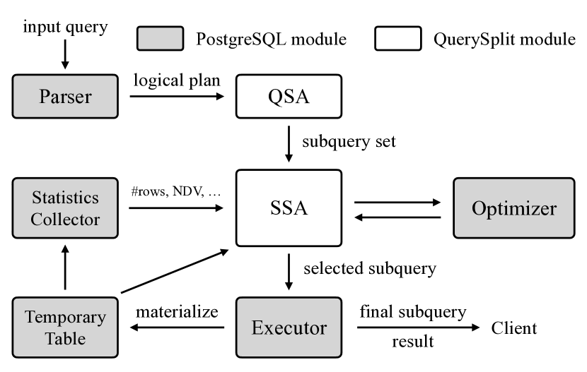
Figure 9. Implementing QuerySplit in PostgreSQL

We implemented the QuerySplit algorithm in PostgreSQL 12.3 in C. As shown in Figure 9, we included two new modules: the Query Splitting Algorithm (QSA) module and the Subquery Selection Algorithm (SSA) module. The data flow is redirected accordingly to perform subquery execution and re-optimization.

Specifically, the QSA module receives a logical plan from the built-in parser and runs the RCenter-based algorithm (Section 4.1) to produce a subquery set that covers the original query. The subqueries in the set are logical plans of the same type as the input of QSA. The subquery set is then sent to the SSA module for execution.

Upon receiving the subquery set, the SSA module starts a loop to consume one subquery at each iteration. As described in Section 4.2, the SSA computes the cost function $\Phi$ for each subquery and sends the one with the smallest cost to the execution engine. During this process, the SSA invokes PostgreSQL’s native optimizer on each subquery to obtain its execution time estimation (i.e., $\textbf{C}(q)$) and its output size estimation (i.e., $\textbf{S}(q)$).

The execution result of the selected subquery (except for the last one) is materialized in a memory buffer by setting the output destination to a temporary table in PostgreSQL. The materialized table is then sent to the Statistics Collector, where a set of PostgreSQL’s native routines are performed to compute the basic statistics about the table such as the number of rows, number of distinct values, histograms, etc. After the statistical analysis, both the temporary table and its associated statistics are sent back to the SSA module to update the remaining “overlapping” subqueries, preparing for the next iteration.

The source code of QuerySplit-integrated PostgreSQL is available on Github through the anonymous link in (Anonymous, 2022).

6. Evaluation

The evaluation of QuerySplit is organized as follows. In Section 6.2, we first examine the policies proposed in Section 4 for the QSA and SSA algorithms. Because the cost function in SSA relies on the optimizer’s output, we then investigate the robustness of our algorithm against varying cardinality estimation errors. Next, we show our main results in Section 6.3, where we compare the end-to-end performance of QuerySplit to that of existing baselines using the Join Order Benchmark (JOB) (Leis et al., 2015). A follow-up study on whether to collect run-time statistics on the materialized intermediate results is presented in Section 6.4 to show the trade-offs. In Section 6.5, We investigate whether the cost functions proposed in Section 4.2 can boost the performance of existing re-optimization algorithms. In Section 6.6, we conduct detailed case studies to provide further insights about the reasons why QuerySplit outperforms the baselines in a majority of situations.

6.1. Workload & Experiment Setup

• Join Order Benchmark (JOB) JOB is a collection of manually-created queries over the IMDB data set (IMD, 2022). It has been widely used in prior work to evaluate the optimizer in relational database management systems (DBMSs)  (Cai et al., 2019; Hertzschuch et al., 2021; Perron et al., 2019). JOB is known to have more complex queries than the standard TPC-H (TPC, 2022b) and is preferable for stress-testing the optimizer. There are a total of 113 queries in JOB with 91 of them returning non-empty results. We use these 91 queries in our evaluation. By default, we build a B+tree index for each primary key and foreign key appearing in the schemas.

• Decision Support Benchmark (DSB) DSB extends the standard TPC-DS benchmark (TPC, 2022a) with data skews (Ding et al., 2021). There are 52 queries (15 SPJ and 37 Non-SPJ) in DSB. We set the scale factor to 5 in the evaluation.

• TPC-H TPC-H (TPC, 2022b) is the standard for benchmarking analytical queries by convention. It follows a star-schema and contains 22 (Non-SPJ) queries. We set the scale factor to 3 in the evaluation.

All experiments are performed on a server equipped with an Intel®Core®i9-10900K CPU (3.70 GHz) and 128 GB of DRAM. Similar to QuerySplit, all the baseline algorithms are also implemented in PostgreSQL. We use the same parameter configuration in PostgreSQL across all solutions. We set the max_parallel_workers to 0 to guarantee a serial execution of the queries in the workload. The effective_cache_size is set to 8 GB. Other parameters follow the PostgreSQL default. The execution of each query times out after 1000 seconds. We repeat each experiment three times and report the average measurements.

6.2. Policies in QSA & SSA

The default policy for subquery generation (i.e., QSA) in QuerySplit is RCenter. To show its efficiency, we introduce two alternative strategies, named ECenter and MinSubquery. As the name suggests, ECenter is the dual of RCenter: the directed join graph in ECenter has all edges reversed (i.e., from a Relationship to an Entity), making the Entity relation at the center of each generated subquery. The other alternative MinSubquery refers to the strategy of dividing the query into minimum-sized subqueries. For each join predicate in the original query, we construct a subquery containing only the involved relations with their corresponding filter conditions, thus creating the smallest join units.

For the cost function $\Phi$ used to determine the subquery execution order (i.e., SSA), besides the five candidates proposed in Table 2, we introduce an additional baseline global_deep that orders the subqueries according to the global physical plan. At each QuerySplit iteration, we choose the deepest join operator in the global plan tree and obtain the involved relation set R. The algorithm then searches the subquery set and finds the one(s) whose relation set is a superset of R. If multiple subqueries satisfy the requirement, the algorithm randomly picks a subquery to send for execution. Notice that QuerySplit with the global_deep SSA policy is different from executing the global plan directly because the subquery set is not derived from the global plan.

Table 3. JOB execution time for different combinations of QSA and SSA policies

	RCenter	ECenter	MinSubquery
$\Phi_{1}$: $\textbf{C}(q)$	421	378	463
$\Phi_{2}$: $\textbf{C}(q)\cdot\log(\textbf{S}(q))$	327	349	428
$\Phi_{3}$: $\textbf{C}(q)\cdot\sqrt{\textbf{S}(q)}$	328	339	418
$\Phi_{4}$: $\textbf{C}(q)\cdot\textbf{S}(q)$	295	350	427
$\Phi_{5}$: $\textbf{S}(q)$	348	407	474
global_deep	356	413	401

Table 3 shows the execution time of the JOB workload using QuerySplit with different combinations of QSA and SSA policies. For QSA policies, RCenter consistently outperforms the others (except for $\Phi_{1}$). This result confirms that keeping more non-expanding operators in subqueries is beneficial to re-optimization (the USE paper presents similar findings (Hertzschuch et al., 2021)). The RCenter policy achieves the goal by preserving as much primary-foreign-key joins as possible when splitting the original query.

For SSA policies, $\Phi_{3}$ and $\Phi_{4}$ outperform the others in general. The results indicate that subqueries with both short execution time and small output cardinality should have execution priority in re-optimization, and a more balanced weight assignment between these two metrics tends to improve the query performance. Overall, a combination of RCenter and $\Phi_{4}$ in QuerySplit leads to an outstanding performance of the DBMS, as shown in Table 3.

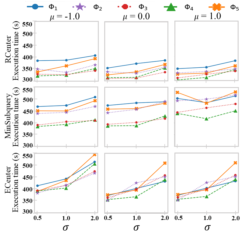
Figure 10. Execution time of QuerySplit on JOB under erroneous cardinality estimations

Robustness test Because the cost functions $\Phi_{1}$ - $\Phi_{5}$ depend on the output from the optimizer, we next test the robustness of these cost functions against cardinality estimation (CE) errors. The experiments are designed in the following way. For each JOB query, we execute every valid subquery from it and record its true output cardinality (true_card). Next, we generate the erroneous cardinality (err_card) by adding a controlled noise to the true cardinality:

$$err\_card=2^{N(\mu,\sigma^{2})}*true\_card$$

where $N(\mu,\sigma^{2})$ represents a normal distribution with $\mu$ as the mean and $\sigma$ as the standard deviation. We then inject the erroneous cardinalities into PostgreSQL’s optimizer via the method proposed by Cai et al. (Cai et al., 2019) so that we can control the quality of the cardinality estimations (CE).

Figure 10 shows the time of executing the JOB workload under the aforementioned different QuerySplit policies with a varying mean and standard deviation of the injected CE noise.

Regardless of the choice of cost functions, modest errors (i.e., $\sigma=0.5,1,2$) in cardinality estimation have a small negative impact on the query performance when QuerySplit adopts the FK-Center or MinSubquery QSA policy. The PK-Center policy is more sensitive to inaccurate cardinalities because a PK-Center subquery is more likely to include multiple large FK-relations, where a miscalculation of the join cardinality could incur an unrecoverable penalty. When the injected CE error becomes large (i.e., $\sigma=4$, which means $Prob$(CE error ¿ $1500\%$) ¿ $30\%$), QuerySplit is no longer robust no matter what QSA and SSA strategies it selects. Because a policy combination of FK-Center and $\Phi_{4}$ outperforms the other pairs consistently under modest CE errors, we set both policies as the default in subsequent experiments.

6.3. A Comparison to Baseline Solutions

In this section, we compare QuerySplit against the following baselines, including four re-optimization algorithms and two approaches to improve cardinality estimation.

• Default: PostgreSQL with the default optimizer.

• Optimal: PostgreSQL with an “ideal” optimizer. We provide the optimizer with the accurate cardinality of every possible intermediate result so that it generates an optimal plan. This serves as the upper-bound for all the evaluated approaches. Note that the “optimality” here is with respect to perfect cardinality estimates.

• Reopt: A re-optimization algorithm that triggers the optimizer at each pipeline breaker if it detects that the deviation between the true statistics and the estimation exceeds a threshold (Kabra and DeWitt, 1998).

• Pop: A re-optimization algorithm extending Reopt where the optimizer is triggered aggressively in more situations including at nested-loop join operators (Markl et al., 2004).

• IEF: Incremental Execution Framework (IEF) by Neumann and Galindo-Legaria (Neumann and Galindo-Legaria, 2013) is an adaptive query processing framework where query executions halt at pre-determined places in the global plan to remove uncertainty in cardinality estimation errors.

• Perron19: A most recent study on the effectiveness of re-optimization (Perron et al., 2019). In the original paper, the authors compare the true cardinality of each operator with the estimated value obtained from the EXPLAIN command. They then materialize the intermediate results of those operators with large CE errors and re-execute the query to study the performance trade-offs. Because it is impractical to get a global view of the true cardinalities by executing the query in advance, we modified the algorithm by setting a relative threshold (e.g., estimation error is $32\times$ off compared to collected statistics) as the run-time re-optimization trigger.

• USE, Pessi.: USE (Hertzschuch et al., 2021) and Pessimistic Cardinality Estimation (Pessi.) (Cai et al., 2019) provide robust cardinality estimation using sketches. Although USE forms subqueries during query optimization, its execution is non-adaptive.

• FS: A robust query processing technique that considers both cost and plan robustness (i.e., insensitive to cardinality estimation errors) during query optimization (Wolf et al., 2018a).

• OptRange: An algorithm that derives the range of estimated cardinalities where the current plan stays optimal (Wolf et al., 2018b). This can serve as a heuristic to reduce unnecessary re-optimizations.

• NeuroCard, DeepDB, MSCN: state-of-the-art learned cardinality estimation algorithms, where NeuroCard (Yang et al., 2020) and DeepDB (Hilprecht et al., 2019) are trained directly against the data while MSCN (Kipf et al., 2018) requires a set of training queries. These algorithms, however, have limited support to string columns.

For baselines that do not provide a PostgreSQL integration, we implemented them according to the paper with the best effort. Implementation details can be found in Appendix B. For each algorithm, we evaluated two index states: (1) indexes are built for primary key (Pk) columns only, and (2) indexes are built for primary key (Pk) and foreign key (Fk) columns.

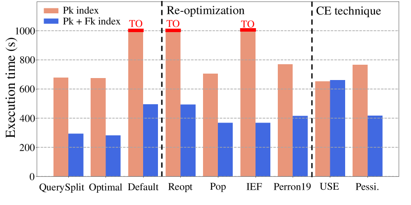
Figure 11. Execution time of JOB for QuerySplit and different baselines (TO = timeout)

6.3.1. Join Order Benchmark

Figure 11 reports the end-to-end execution time of the JOB workload for QuerySplit and the above baselines. In both Pk index only and Pk + Fk index cases, QuerySplit achieves the shortest execution time compared to the prior solutions. The performance improvements are more significant when both primary-key and foreign-key indexes are included (which is the default in JOB) because the (sub)plan qualities between different algorithms diverge more with an enlarged optimization space.

Notice that the performance difference between QuerySplit and Optimal is very small ($<4\%$), indicating that QuerySplit is able to identify and quickly converge to an optimal plan. It also shows that the re-optimization overhead in QuerySplit is modest. The four re-optimization baselines achieve a certain amount of improvement over the Default, but they are still noticeably slower than the optimal. This is because they are all held back by the initial physical plan in the re-optimization process. We provide case studies in Section 6.6 to demonstrate QuerySplit’s advantages in detail.

Compared to the robust query processing baselines (i.e., USE , Pessi, FS, and OptRange), QuerySplit still exhibits significant performance advantages, especially when both primary key and foreign key columns have indexes built (i.e., the blue bars in Figure 11). This is because robust query processing algorithms tend to settle down with plans that are insensitive to cardinality estimation errors and thus miss the opportunity to approach plans that are closer to the optimal. Meanwhile, learned cardinality estimation (i.e., NeuroCard, DeepDB, and MSCN) achieves limited performance improvement because JOB contains many string columns where the learned cardinality estimators fail to handle: they have to fall back to PostgreSQL’s default in those cases. These results confirm the finding in Perron et al. (Perron et al., 2019) that re-optimization is likely to be more effective and efficient than refining CE in improving query performance.

Table 4. Materialization frequency and memory usage of re-optimization algorithms

Algorithms	Avg mem per	Avg mat. freq.	Total mem per
	subquery (MB)	per query	query (MB)
QuerySplit	5.79	2.66	15.40
Reopt	43.31	0.21	9.09
Pop	7.01	4.62	32.39
IEF	14.59	3.11	45.37
Perron19	10.99	6.59	72.42

Table 4 shows the materialization frequency and the associated memory usage of each of the re-optimization algorithms. Compared to the baselines, QuerySplit has the lowest memory consumption per subquery (i.e., per re-optimization iteration) because the RCenter-based QSA preserves as many non-expanding operators in the subqueries as possible. QuerySplit also has the second lowest re-optimization frequency per query. Reopt achieves the lowest because it only triggers re-optimization at pipeline breakers with large CE errors. Overall, except for Reopt that adopts an over-conservative strategy, the materialization memory cost of QuerySplit is significantly lower than that of the other competitors.

6.3.2. TPC-H

Unlike JOB, TPC-H serves as a worst-case benchmark for QuerySplit because it follows the star-schema pattern and all of its queries are Non-SPJ queries. Figure 12 shows the results for TPC-H. Note that we only include the baseline approaches that support Non-SPJ queries in the figure. QuerySplit still produces the fastest plans among the baselines, although the performance improvements are much smaller than those in JOB. As discussed in Section 4.1, re-optimization is often unnecessary for star-schema queries because the optimizers are less likely to make serious mistakes. QuerySplit outperforms existing re-optimization algorithms, nonetheless, because QuerySplit triggers a (“useless”) re-optimization less frequently in TPC-H.

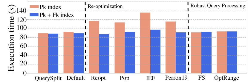
Figure 12. TPC-H Execution Time

6.3.3. Decision Support Benchmark

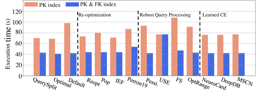
Figure 13. DSB Execution Time – SPJ Queries

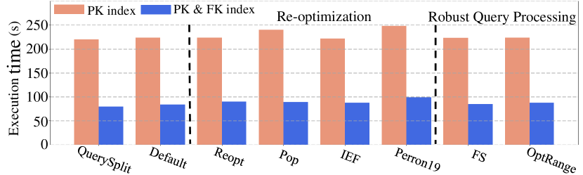
Figure 14. DSB Execution Time – Non-SPJ Queries

Finally, we show the evaluation results for DSB, a mostly star-schema benchmark containing both SPJ and Non-SPJ queries. For SPJ queries, as shown in Figure 13, QuerySplit is close to the “optimal” and outperforms the baselines, especially in the Pk-index-only setting. Compared to the JOB results, the overall benefit of re-optimization in DSB is less remarkable because of the star-schema pattern. Notice that the learned cardinality estimation algorithms become more effective because DSB has fewer string attributes involved in the queries. The results for Non-SPJ queries of DSB (Figure 14) are similar to those of TPC-H. Although QuerySplit targets at JOB-like workloads that are proven to be challenging for optimizers (Leis et al., 2015), our experiments with TPC-H and DSB show that QuerySplit keeps a robust performance consistently, thanks to its low re-optimization overhead.

6.4. Collecting Statistics Or Not?

We continue with a follow-up study on whether collecting statistics on the materialized intermediate results is beneficial for each re-optimization algorithm. The statistics include the number of distinct values, most common values and their frequencies, equal-width/depth histograms, etc. Note that the basic row count is already obtained during the result materialization.

Collecting the above statistics requires extra table scans in PostgreSQL. Such an overhead may not exist if the DBMS is sophisticated enough to generate the statistics while materializing the intermediate results. Nevertheless, all the four re-optimization baselines choose to collect statistics at runtime by default. The reasoning is that collecting these statistics is going to help plan future subqueries because the optimizer has little knowledge of the newly materialized relation(s).

We repeat the JOB experiments for the re-optimization algorithms in two different settings: (1) collecting the statistics for every materialized intermediate result, and (2) disabling the statistics collector and only passing along the row count to the optimizer.

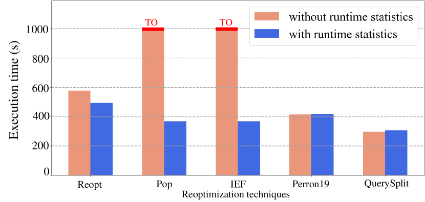
Figure 15. JOB execution time with and without high-level statistics

Figure 15 shows the benchmark results. Surprisingly, collecting statistics at runtime has no effect (even a slightly negative effect) on the overall query performance in Perron19 and QuerySplit, despite the performance of other algorithms depending heavily on those statistics. This is because each subquery in Perron19 only involves at most two relations and is, therefore, less likely for the optimizer to make mistakes due to the lack of statistics. For QuerySplit, each subquery mostly contains primary-foreign-key joins. Because PostgreSQL’s optimizer does not use any additional statistics other than the row count of the primary-key table to estimate the cardinality of such a join, collecting the statistics provides little benefit for the optimizer to generate a better plan.

The above experiments show that whether to collect statistics during re-optimization should not be a “no-brainer”. The decision depends heavily on the re-optimization algorithm and the quality of the system’s native optimizer.

6.5. Existing Re-optimization Algorithms with New Cost Functions

We investigate whether the cost functions proposed in Section 4.2 can boost the performance of existing re-optimization algorithms in this section. We repeat the JOB experiments on Re-opt, Pop, IEF, and Perron19 and use our cost functions (i.e., $\Phi_{1}-\Phi_{5}$) to determine which subquery to execute first. Table 5 presents the benchmark execution times.

Table 5. JOB execution time for existing re-optimizations algorithms with cost functions from QuerySplit.

	Reopt	Pop	IEF	Perron19
$\Phi_{1}$: $\textbf{C}(q)$	488	406	877	412
$\Phi_{2}$: $\textbf{C}(q)\cdot\log(\textbf{S}(q))$	482	479	835	420
$\Phi_{3}$: $\textbf{C}(q)\cdot\sqrt{\textbf{S}(q)}$	475	480	855	418
$\Phi_{4}$: $\textbf{C}(q)\cdot\textbf{S}(q)$	483	485	857	417
$\Phi_{5}$: $\textbf{S}(q)$	492	487	800	415
Original	493	401	367	416

Overall, simply applying the proposed cost functions to existing re-optimization algorithms brings little benefit. IEF, in particular, experienced major performance degradation because the new cost functions break IEF’s optimization strategy of prioritize subqueries with a high uncertainty in cardinality estimation. These experiments demonstrate that a “wise” cost function alone is incapable of compensating for a sub-optimal subquery division in a re-optimization algorithm.

6.6. Insights into QuerySplit

In this section, we provide a deeper analysis on the reasons why QuerySplit outperforms existing re-optimization algorithms. An intuition is that QuerySplit prioritizes the execution of subqueries that produce smaller intermediate results and, thus, postponing potential large joins by as much as possible.

To verify this, we plot two sets of “timelines” for each JOB query, where the X-axis is the count of completed re-optimization iterations. For the first set of timelines, we monitor the size of the intermediate result at each re-optimization iteration for each evaluated algorithm (Reopt is omitted because of poor performance). For the second set of timelines, we plot the execution time for the corresponding subquery at each iteration.

When comparing QuerySplit against Pop, IEF, Perron19, and Optimal (for reference), we summarized four representative categories out of the 91 JOB queries:

• Avoided Large Joins: QuerySplit successfully avoided performing large join(s) that appears in other re-optimization algorithms.

• Delayed Large Joins: QuerySplit postponed the large join(s) to later iterations with (hopefully) a smaller input size and a smaller impact on the performance of other subqueries.

• No Difference: The timeline patterns and the performance are similar between QuerySplit and other re-optimization algorithms.

• Worse: A rare case where QuerySplit unexpectedly produced large intermediate results and performed worse than the others.

We next provide detailed case studies for each category.

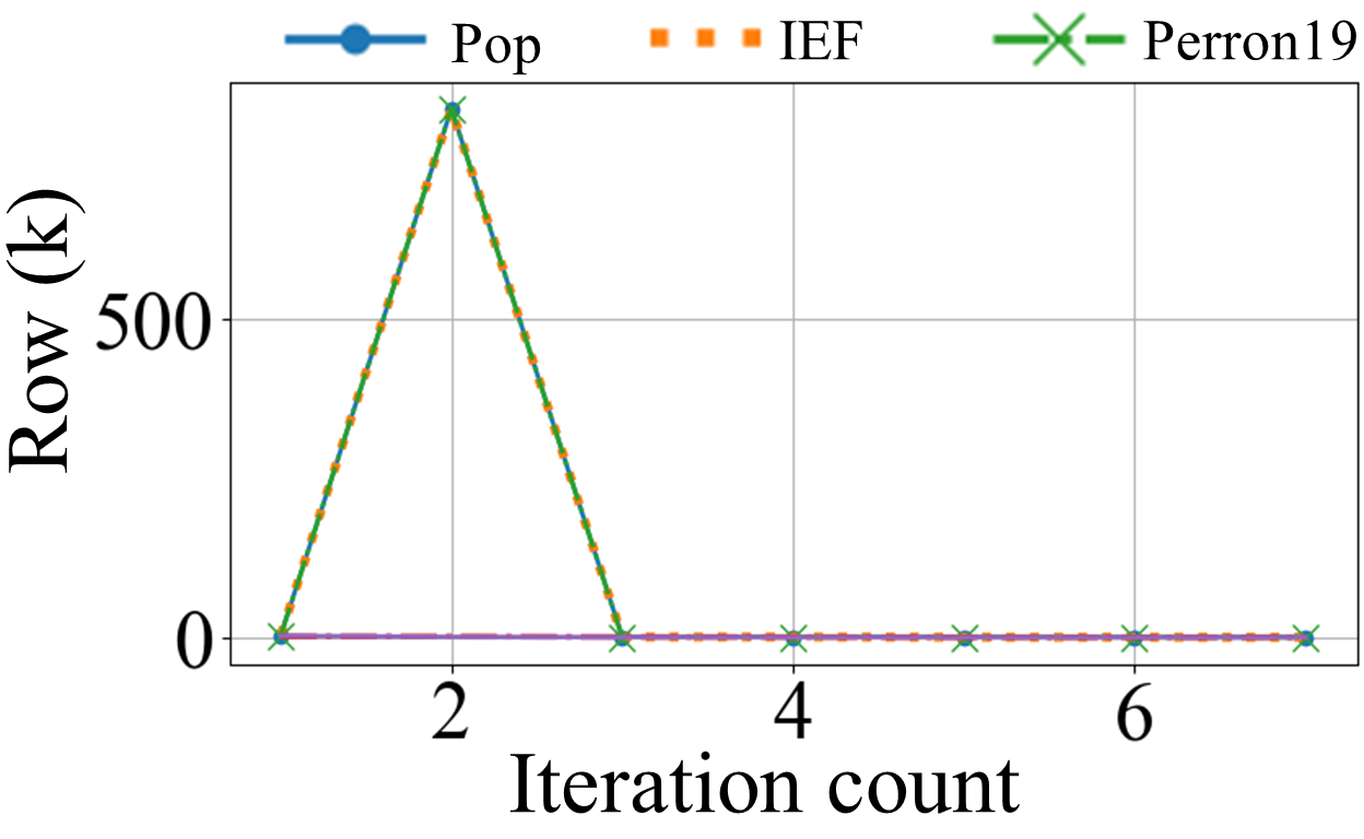
(a) Result size at each iteration

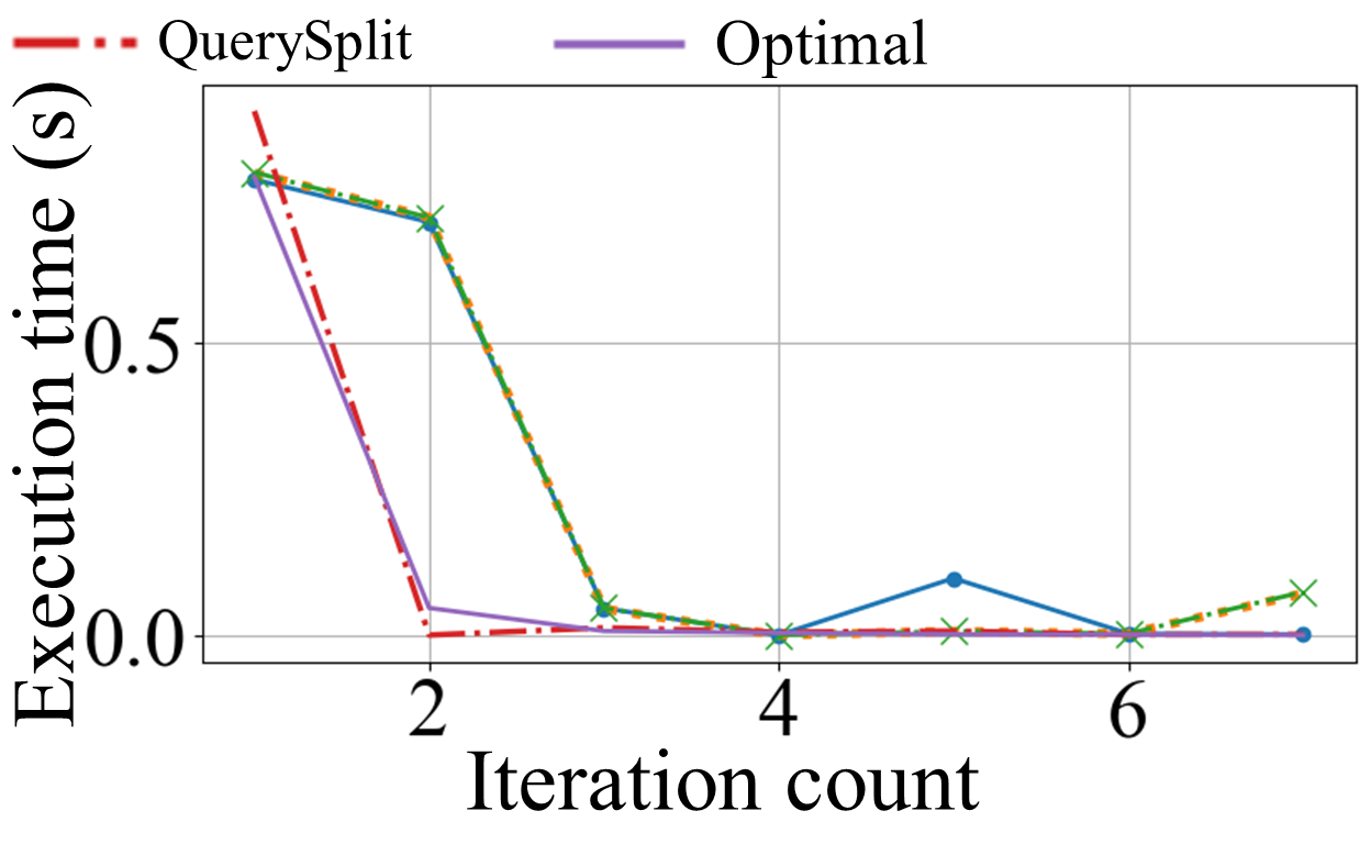
(b) Execution time at each iteration

Figure 16. Re-optimization Timelines for the “Avoided Large Join” Category

6.6.1. Avoided Large Join

Figure 16 shows the intermediate result size and execution time at each re-optimization iteration for a representative query in this category. We can see that Pop, IEF and Perron19 execute a subquery that generates a large intermediate result close to 1M rows in an early (2nd) iteration. The execution time of this subquery is also large, as shown in Figure 16(b). The reason is that both algorithms rely on a bad initial plan (generated by the PostgreSQL’s default optimizer) that decides to execute this large join early because of cardinality estimation errors. On the other hand, QuerySplit successfully avoided the large join by first executing simple subqueries that imposed highly-selective filters on the large input relations. As expected, these wise choices perfectly overlap with the optimal plan.

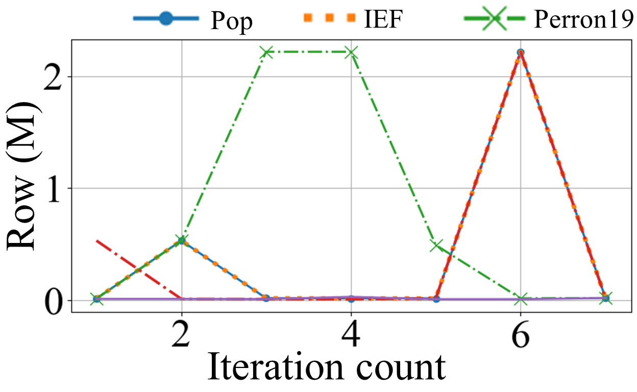
(a) Result size at each iteration

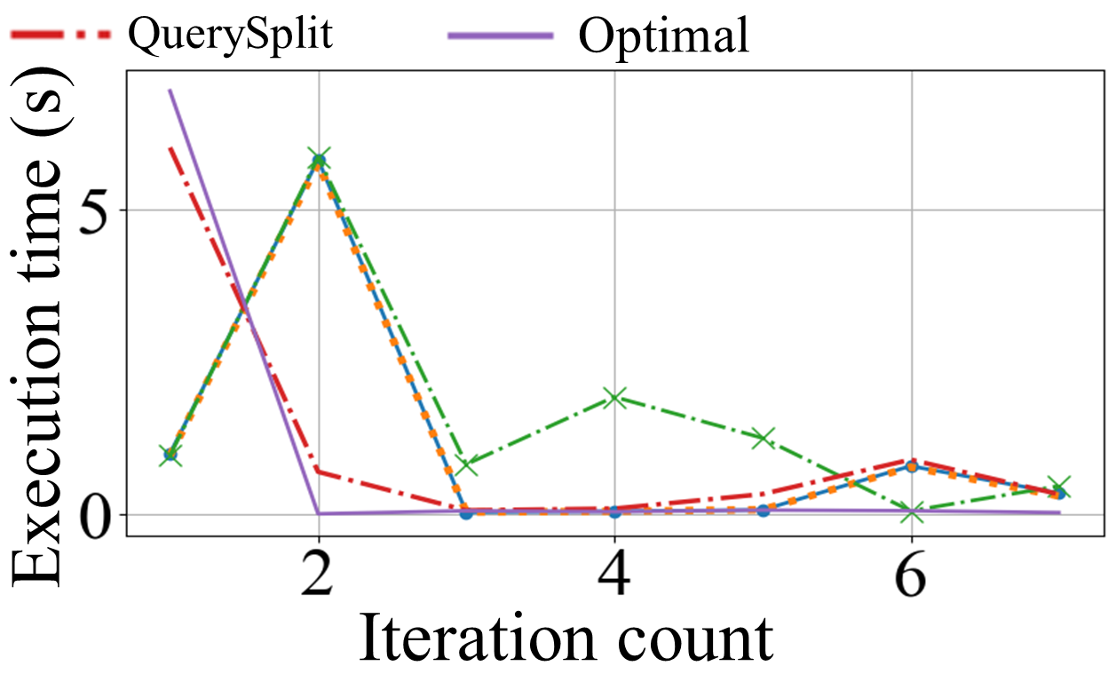
(b) Execution time at each iteration

Figure 17. Re-optimization Timelines for the “Delayed Large Join” Category

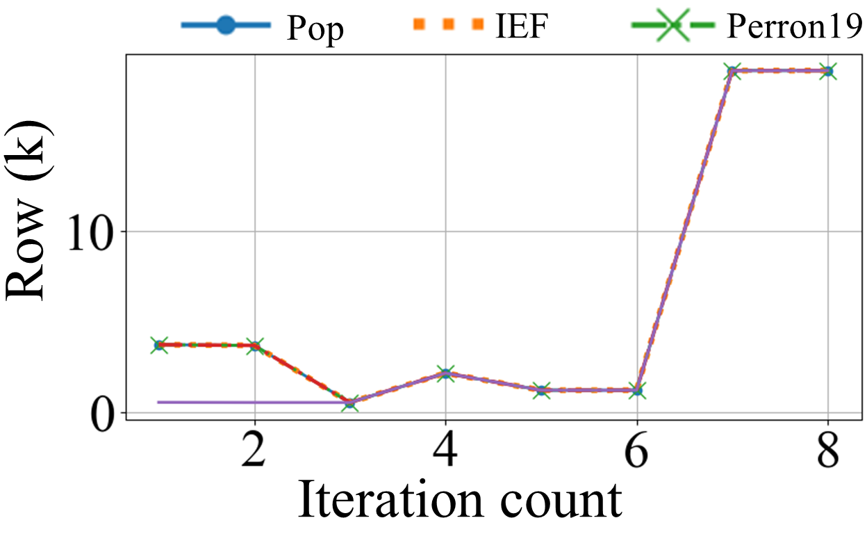
(a) Result size at each iteration

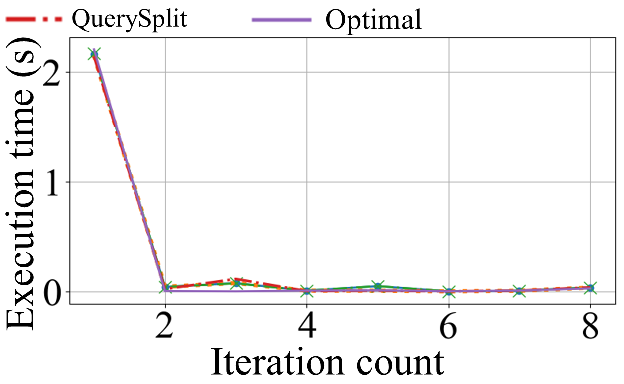
(b) Execution time at each iteration

Figure 18. Re-optimization Timelines for the “No Difference” Category

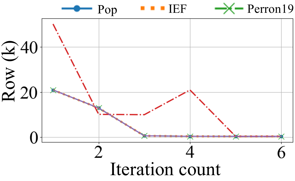
(a) Result size at each iteration

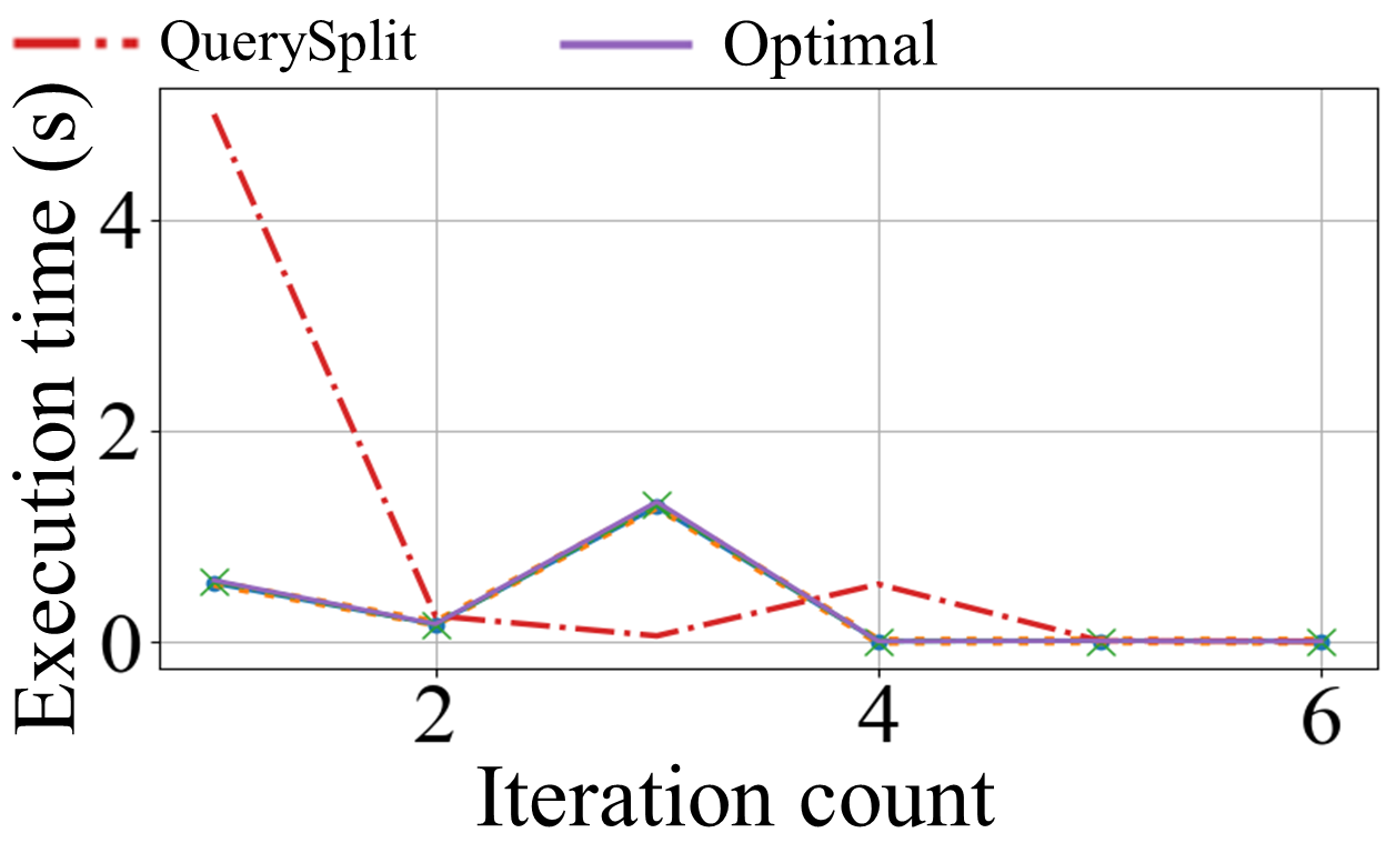
(b) Execution time at each iteration

Figure 19. Re-optimization Timelines for the “Worse” Category

6.6.2. Delayed Large Join

A representative set of re-optimization timelines for this category is presented in Figure 17. The observation is that all of the re-optimization algorithms execute at least one subquery that generates a large intermediate result. QuerySplit, however, delays such an execution by as much as possible because the cost function $\Phi_{4}$ used in the SSA module has a strong preference for subqueries that are “easy” and produce small outputs. Delaying the execution of large joins reduces the probability of letting them slow down additional subqueries. As shown in Figure 17(a), because Perron19 executes a large join as early as in the third iteration, its succeeding iteration suffers from large input and output sizes again due to the ripple effect.

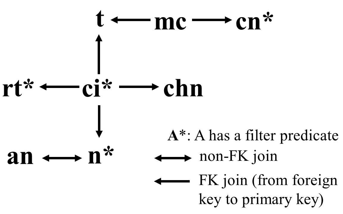
(a) Join Graph of JOB query $\#$9c

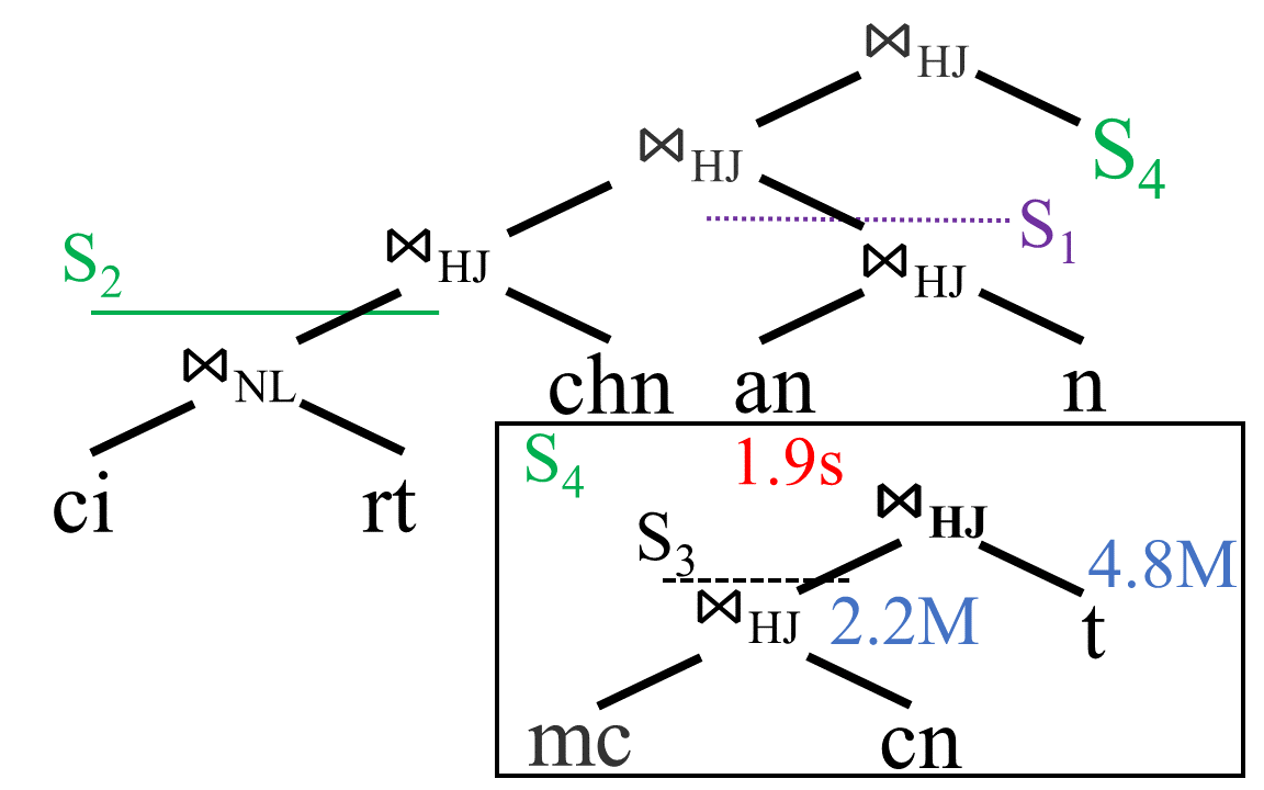
(b) Perron19

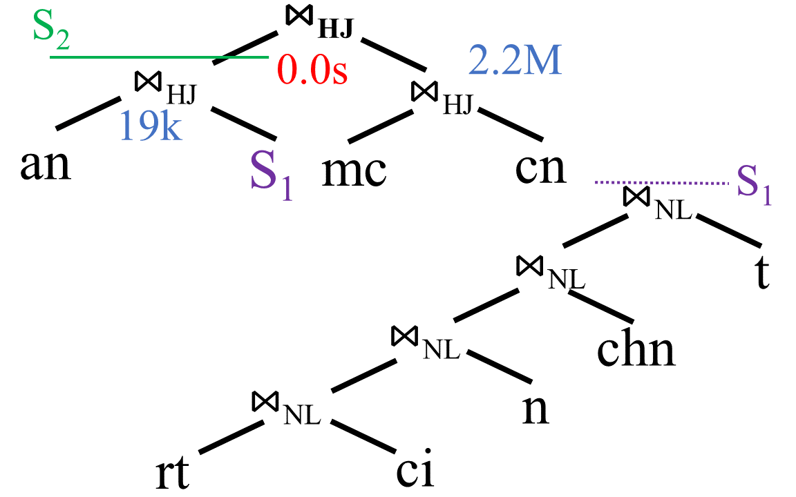
(c) QuerySplit

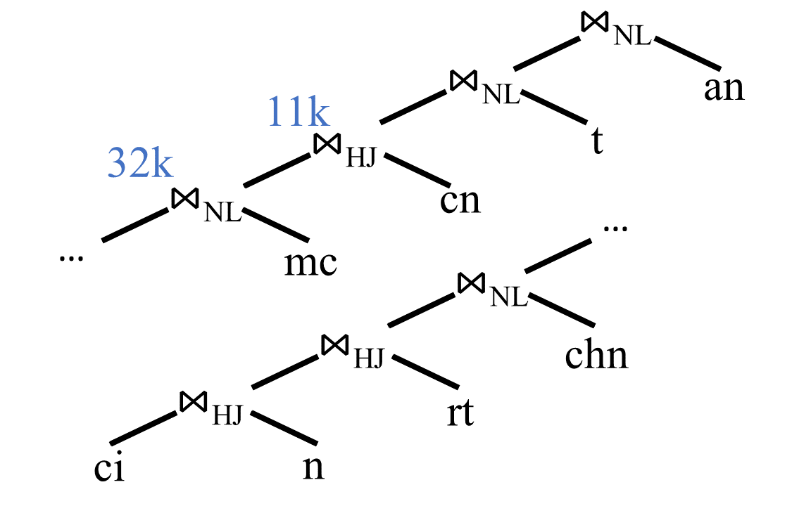
(d) Optimal

Figure 20. (a)The join graph of JOB query #9c and (b)(c) execution processes of the example query in Delayed Large Joins (The blue and red text represents the actual cardinality and the execution time respectively, and the cutting lines represent where the re-optimization is triggered)

We show the concrete query in Figure 20 for a case study. Figure 20(a) shows the join graph of the JOB query. The (effective) execution plan for Perron19, QuerySplit, and Optimal are illustrated in Figures 20(b), 20(c) and 20(d), respectively. Both Perron19 and QuerySplit encounter the large join mc $\Join$ cn that produces an output relation x with a size of $2.2$M) in one of their subqueries. However, because Perron19 performs this join too early, its subsequent join (i.e., x $\Join$ t) becomes even larger ($2.2$M $\times$ $4.8$M) and takes $1.9$s to complete. On the contrary, QuerySplit delays the execution of mc $\Join$ cn towards the end and gets rewarded by having a much smaller-scale subsequent join ($2.2$M $\times$ $19$K) that can be finished in less than $0.1$s.

An interesting observation is that the large mc $\Join$ cn is completely avoided in the optimal plan. By comparing the plans between QuerySplit and Optimal carefully, we found that the decisive mistake made by QuerySplit is choosing to execute an $\Join$ $S_{1}$ first instead of mc $\Join$ $S_{1}$. This is because an $\Join$ $S_{1}$ has a much smaller estimated cost from the optimizer (i.e., $46$K vs. $132$K for $\textbf{C}(q)$) and a similar estimated output size (i.e., $19$K vs. $18$K for $\textbf{S}(q)$) compared to cn $\Join$ mc $\Join$ $S_{1}$. A more sophisticated cost function $\Phi$ might be able to further reduce these undesirable decisions. Nevertheless, we notice that the differences in query execution time between QuerySplit and Optimal are small despite our algorithm generating a larger intermediate result.

6.6.3. No Difference

As shown in Figure 18, in this category, all the re-optimization algorithms converge to the same (effective) execution plan. This is because the cardinality estimation of these queries is relatively accurate to prevent the optimizer and the re-optimizing process from making mistakes.

6.6.4. Worse

This is a relatively infrequent category where QuerySplit is slower than the other competitors because of a bad decision leading to a large intermediate result. The re-optimization timelines of a representative query are shown in Figure 19. QuerySplit consumes more time and produces larger outputs than the others in the first and fourth iterations.

We found that almost all the bad cases are small queries, each getting split into only two subqueries in QuerySplit. Figure 21 shows an example. Again, Figure 21(a) shows the join graph of the JOB query. We depict the (effective) execution plan for QuerySplit and IEF in Figures 20(b) and 20(c), respectively. Other alternative algorithms have the same plan as IEF.

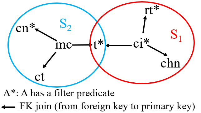
(a) Join graph of JOB query $\#$15c

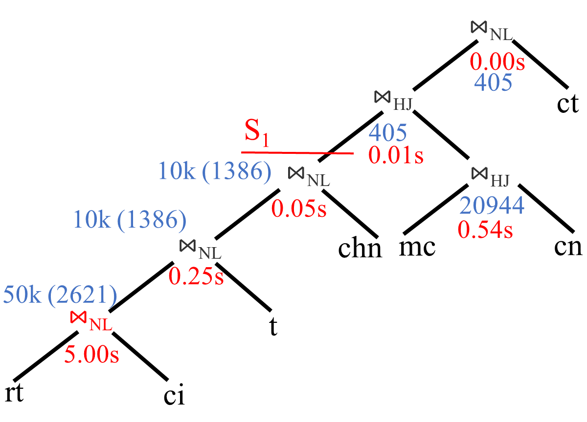
(b) Execution process of QuerySplit

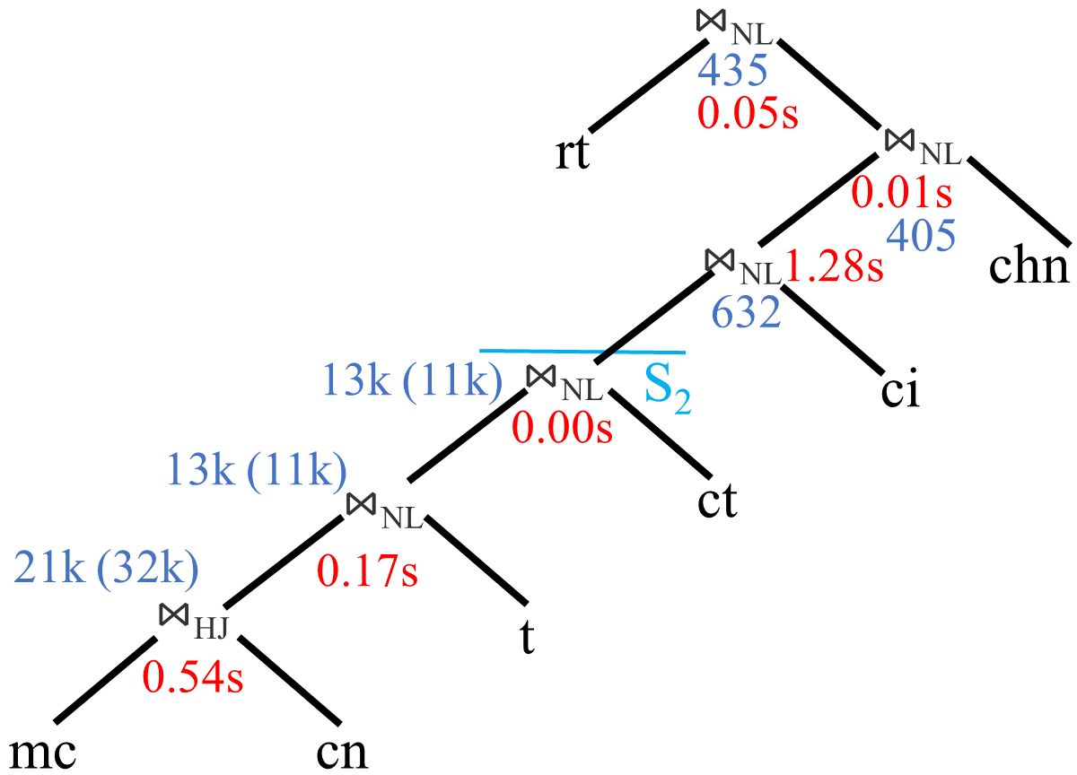
(c) Execution process of IEF

Figure 21. (a) The join graph of JOB query #15c and (b)(c) the execution processes of the example queries in Worse (The blue text outside the bracket and in the bracket represents the actual cardinality and the estimated cardinality respectively, the red text represents the execution time, and the cutting lines represent where the re-optimization is triggered)

We observe that both QuerySplit and IEF generate the identical subqueries: S₁ $=$ ci $\Join$ rt $\Join$ t $\Join$ chn and S₂ $=$ mc $\Join$ cn $\Join$ t $\Join$ ct. The difference is that QuerySplit chose to execute S₁ first, while IEF chose to prioritize S₂. This is because PostgreSQL’s optimizer makes a huge mistake in estimating the cardinality of S₁. Such a mistake “tricks” QuerySplit into believing that S₁ has a much smaller output size than S₂ ($1386$ vs. $11$K), an advantage outweighing the difference between their execution cost ($5.3$s vs. $0.71$s). Considering the true cardinality for S₁ and S₂ are similar ($10$K vs. $13$K), QuerySplit made a bad decision in executing the heavier S₁ first.

The lesson learned (for future improvements) is that fine-grained subqueries are preferred in re-optimization because they are less likely to cause devastating cardinality estimation errors even with a mediocre optimizer.

6.6.5. Summary

Table 6. Frequencies and the average performance effect of the four categories of JOB queries

Category	Frequency	Average Perf. Effect
Avoided Large Join	40 / 91	40.5%
Delayed Large Join	23 / 91	21.7%
No difference	18 / 91	3.8%
Worse	10 / 91	-39.5%

Table 6 presents the query count of each of the above categories out of the 91 JOB queries. The average performance effect refers to QuerySplit’s relative performance improvement over the best alternative algorithm. The query counts show that $\approx 70\%$ of the queries belong to the first two categories where QuerySplit outperforms alternative re-optimization algorithms by a sizeable gap. Although queries get slowed down significantly in the Worse category, it has a small effect on the overall benchmark performance because such a query is infrequent and the query itself is small.

7. Related Work

There are two research directions related to our work: (a) adaptive query processing and (b) cardinality estimation techniques. We review existing work in these directions in the following two subsections.

7.1. Adaptive Query Processing

Adaptive query processing is a research direction with a long history. Babu and Bizarro (Babu and Bizarro, 2005) have conducted a comprehensive review of existing works in this direction. According to their investigation, adaptive query processing techniques can be broadly categorized into three families: plan-based system (re-optimization), routing-based system and continuous-query-based system.

7.1.1. Re-optimization

A re-optimization system monitors the execution of the current plan and re-optimizes the plan whenever the actual condition differs significantly from the estimations made by the optimizer.

As far as we know, Reopt is the first research that proposed the idea of re-optimization. Reopt (Kabra and DeWitt, 1998) adds statistics collecting operators after pipeline breakers (e.g., hash or sort) in the physical plan. When a deviation is detected, the database calculates the benefit of re-planning the remaining part of the query and compares it with the cost of re-optimization. Pop (Markl et al., 2004) is very similar to Reopt, except that Pop can trigger re-optimization in more join nodes, like the outer side of nest-loop join. Instead of deciding when to materialize based on the node type, incremental execution framework (IEF) (Neumann and Galindo-Legaria, 2013) chose the node in the global physical plan which has the maximal estimation error on cardinality to materialize. The estimation error on cardinality is estimated based on the statistics and assumptions used. Recently, Perron et al. (Perron et al., 2019) conducts a simulation study to investigate the effectiveness of re-optimization. They use the EXPLAIN command to evaluate cardinality estimation error, and materialize the intermediate results that deviate too much from estimation as a temporary table. Their result shows that re-optimization can sharply improve the execution time in PostgreSQL. Moreover, Databricks and Spark extended re-optimization to the Mapreduce background (Wenchen et al., 2020). They re-optimized at shuffle or broadcast exchange, and optimized not only join order and physical operator selection, but also shuffle partitions.

Compared to the QuerySplit framework, the above methods choose the subtree of the global physical plan to execute. Such a strategy can go wrong when the referencing global plan deviates largely from an optimal one. And if a bad subplan is chosen, the damage often influences later execution.

7.1.2. Routing-based system

Routing-based systems behave differently compared to traditional RDBMS. They process queries by routing tuples through a pool of operators. The idea of the routing-based system can be traced back to INGRES (Wong and Youssefi, 1976). The most representative work is Eddies (Avnur and Hellerstein, 2000), which adds a new operator called ripple join and can change the join order in ripple joins. Compared to re-optimization, routing-based systems totally abandon the optimizer, making routing algorithms highly dependent on the greedy algorithm and therefore unsuitable for complex queries (Ioannidis et al., 1997; Trummer et al., 2021).

7.1.3. Continuous-query-based System

Continuous-Query-based, or CQ-based, systems are used for queries that will run many times or a very long time, which is prevalent in data stream systems. Compared to other adaptive query processing, CQ-base systems pay attention to the runtime change of stream characteristics and system conditions, rather than cardinality estimation errors of a given query.

7.2. Cardinality Estimation

Cardinality estimation techniques are relevant but orthogonal to our work. QuerySplit benefits from the improvement of cardinality estimation on small joins. Making an optimal plan in each subquery can significantly enhance overall performance.

Cardinality estimation techniques can be categorized into traditional methods and learned methods (Sun et al., 2021), depending on whether machine learning techniques are used.

7.2.1. Traditional Methods

Traditional methods include sketch (Rusu and Dobra, 2008; Cai et al., 2019; Hertzschuch et al., 2021), histogram (Gunopulos et al., 2005) and sampling (Leis et al., 2017; Wu et al., 2016). One particularly related work in this part is USE (Hertzschuch et al., 2021), in which the idea of using non-expanding operators (e.g., filter and Pk-Fk join) is independently proposed. In USE, these operators are prioritized to form subqueries (which is similar to subqueries formed in RCenter). Then, sketch-based cardinality estimation techniques are used to decide the join order between subqueries. However, USE is not an adaptive query processing method, and it uses standard query optimization after conducting the above query transformation.

7.2.2. Learned Methods

Learned methods can be further divided into two categories: data-driven cardinality estimator (Yang et al., 2019; Tzoumas et al., 2011; Gunopulos et al., 2005; Hilprecht et al., 2019; Sun and Li, 2019; Yang et al., 2020; Kipf et al., 2019; Hasan et al., 2020) and query-driven cardinality estimator (Sun and Li, 2019; Stillger et al., 2001; Heimel et al., 2015; Kipf et al., 2018; Park et al., 2020; Marcus et al., 2019; Dutt et al., 2020; Ortiz et al., 2018). The data-driven cardinality estimator approximates the data distribution of a table by mapping each tuple to its probability of occurrence in the table. The query-driven cardinality estimator uses some models to learn the mapping between queries and cardinalities. Although learned methods are indeed more accurate than traditional methods, they often suffer from high training and inference costs (Sun et al., 2021).

8. Conclusion

In this paper, we propose QuerySplit, a re-optimization framework which ignores the potentially misleading global plans and instead extracts subqueries directly from the original logical plan. We proposed a cost function that prioritizes the execution of simple subqueries with small output sizes. Experimental results on Join Order Benchmark showed that QuerySplit outperforms other re-optimization methods and state-of-the-art sketch-based cardinality estimation techniques, and reaches near-optimal execution time.

Appendix A Proof of Theorem 1

This appendix shows the proof of Theorem 1.

Theorem 0.

Let $q(\textbf{{R}},\textbf{{P}})$ be an SPJ query, Q be a set of subqueries of $q$. QuerySplit produces the same output as $q$ if $\textbf{{Q}}\rightharpoonup_{c}q$.

Proof 0.

To begin with, let us introduce several notations:

1. For a set of subqueries $\textbf{{Q}}=\{q_{1}(\textbf{{R}}_{1},\textbf{{P}}_{1}),...,q_{n}(\textbf{{R}}_{n},\textbf{{P}}_{n})\}$, we denote $R(\textbf{{Q}})=\cup_{i=1}^{n}\textbf{{R}}_{i}$, $P(\textbf{{Q}})=\cup_{i=1}^{n}\textbf{{P}}_{i}$.

2. For a set of relations $\textbf{{R}}=\{r_{1},...,r_{n}\}$, we denote $\mathsf{X}_{r\in\textbf{{R}}}=r_{1}\times...\times r_{n}$.

3. For a SPJ query $q(\textbf{{R}},\textbf{{P}})$ and a set of subqueries Q of $q$, we denote the result of $q$ as $E(q)=\sigma_{\textbf{{S}}}(\mathsf{X}_{r\in\textbf{{R}}})$, and the output of the QuerySplit algorithm as $E(\textbf{{Q}})$.

Under these notations, we can rewrite the theorem as: Given a SPJ query $q(\textbf{{R}},\textbf{{P}})$, and a set of subqueries Q of $q$, such that $\textbf{{Q}}\rightharpoonup_{c}q$. Then we have $E(q)=E(\textbf{{Q}})$.
Without loss of generality, we assume that the names of all attributes in R are unique. Under such assumption, we do not need to consider the rename operation when modifying subqueries, and for simplicity we assume that the rename step is skipped.
Now, we start to prove the rewritten theorem by induction on $|\textbf{{Q}}|$.
First, We prove the statement holds when $|\textbf{{Q}}|=1$, in which case $\textbf{{Q}}=\{q_{1}(\textbf{{R}}_{1},\textbf{{P}}_{1})\}$. Apparently the only way that $\textbf{{Q}}\rightharpoonup_{c}q$ is $q_{1}=q$. So the statement clearly holds for $|\textbf{{Q}}|=1$.
Now, assume that the statement holds when $|\textbf{{Q}}|=n-1$. We consider the case of $|\textbf{{Q}}|=n$, $\textbf{{Q}}=\{q_{1}(\textbf{{R}}_{1},\textbf{{P}}_{1}),...,q_{n}(\textbf{{R}}_{n},\textbf{{P}}_{n})\}$.
Without loss of generality, we denote the first executed subquery as $q_{1}(\textbf{{R}}_{1},\textbf{{P}}_{1})$ and discuss two cases: (1) $\forall i>1,\textbf{{R}}_{1}\cap\textbf{{R}}_{i}=\emptyset$ and (2) $\exists i>1,s.t.\textbf{{R}}_{1}\cap\textbf{{R}}_{i}\neq\emptyset$.
Case 1: We first execute $q_{1}$ and materialize its result as relation $m_{1}=E(q_{1})$. Then, because $\forall i>1,\textbf{{R}}_{1}\cap\textbf{{R}}_{i}=\emptyset$, according to the algorithm, we have to add $m_{1}$ to the subquery result set L. After that, we remove $q_{1}$ from Q and have a new subquery set $\textbf{{Q}}^{\prime}=\{q_{2}(\textbf{{R}}_{2},\textbf{{P}}_{2}),...,q_{n}(\textbf{{R}}_{n},\textbf{{P}}_{n})\}$ for the next iteration.
We construct a SPJ query $q^{\prime}(\textbf{{R}}^{\prime},\textbf{{P}}^{\prime})$, where $\textbf{{R}}^{\prime}=\cup_{i=2}^{n}\textbf{{R}}_{i}$ and $\textbf{{P}}^{\prime}=\cup_{i=2}^{n}\textbf{{P}}_{i}$. Apparently, $\textbf{{Q}}^{\prime}\rightharpoonup_{c}q^{\prime}$ and as $|\textbf{{Q}}^{\prime}|=n-1$, by induction hypothesis, $E(q^{\prime})=E(\textbf{{Q}}^{\prime})$.
The final result is the Cartesian product on the elements in L, so we have:

$$E(\textbf{{Q}})=\mathsf{X}_{r\in\textbf{{L}}}=m_{1}\times\mathsf{X}_{r\in(\textbf{{L}}\setminus\{m_{1}\})}=E(q_{1})\times E(\textbf{{Q}}^{\prime})=E(q_{1})\times E(q^{\prime})$$

$$=\sigma_{\textbf{{P}}_{1}}(\mathsf{X}_{r\in\textbf{{R}}_{1}})\times\sigma_{\textbf{{P}}^{\prime}}(\mathsf{X}_{r\in\textbf{{R}}^{\prime}})=\sigma_{\textbf{{P}}_{1}\cup\textbf{{P}}^{\prime}}(\mathsf{X}_{r\in\textbf{{R}}})=\sigma_{\textbf{{P}}}(\mathsf{X}_{r\in\textbf{{R}}})=E(q)$$

Case 2: We denote the set of subqueries that need to be modified after executing $q_{1}$ as $\textbf{{W}}=\{q_{k}(\textbf{{R}}_{k},\textbf{{P}}_{k})\in\textbf{{Q}}:k>1,\textbf{{R}}_{1}\cap\textbf{{R}}_{k}\neq\emptyset\}$.
After we execute $q_{1}$ and materialize its result as relation $m_{1}$, we modify each $q_{i}\in\textbf{{W}}$ and keep $\textbf{{L}}=\emptyset$. We denote these new-formed subqueries as $q^{\prime}_{i}(\textbf{{R}}^{\prime}_{i},\textbf{{P}}^{\prime}_{i})$ and $\textbf{{R}}^{\prime}_{i}=\textbf{{R}}_{i}\setminus\textbf{{R}}_{1}\cup\{m_{1}\}$, $\textbf{{P}}^{\prime}_{i}=\textbf{{P}}_{i}$. These new-formed subqueries form a new set $\textbf{{W}}^{\prime}$.
Now, Q becomes a new subquery set $\textbf{{Q}}^{\prime}=\textbf{{Q}}\cup\textbf{{W}}^{\prime}\setminus\{q_{1}\}\setminus\textbf{{W}}$. Because $\textbf{{L}}=\emptyset$ at this point, when reconstruction finishes, we have $E(\textbf{{Q}})=E(\textbf{{Q}}^{\prime})$.
We construct a new query $q^{\prime}(\textbf{{R}}^{\prime},\textbf{{P}}^{\prime})$, where $\textbf{{R}}^{\prime}=\textbf{{R}}\setminus\textbf{{R}}_{1}\cup\{m_{1}\}$ and $\textbf{{P}}^{\prime}=\cup_{i=2}^{n}\textbf{{P}}_{i}$. We will prove that $E(q^{\prime})=E(\textbf{{Q}}^{\prime})$ and $E(q^{\prime})=E(q)$, hence finishes the proof. To prove $E(q^{\prime})=E(\textbf{{Q}}^{\prime})$, by induction hypothesis, we only need to show that $\textbf{{Q}}^{\prime}\rightharpoonup_{c}q^{\prime}$ and $|\textbf{{Q}}^{\prime}|=n-1$.

• Apparently, $R(\textbf{{Q}}^{\prime})=R(\textbf{{Q}})\setminus\textbf{{R}}_{1}\cup\{m_{1}\}=\textbf{{R}}\setminus\textbf{{R}}_{1}\cup\{m_{1}\}=\textbf{{R}}^{\prime}$. And because $P(\textbf{{Q}}^{\prime})=\cup_{i=2}^{n}\textbf{{P}}_{i}=\textbf{{P}}^{\prime}$, $P(\textbf{{Q}}^{\prime})$ logical implies $\textbf{{P}}^{\prime}$, so $\textbf{{Q}}^{\prime}\rightharpoonup_{c}q^{\prime}$.

• Notice that $\textbf{{W}}\subseteq\textbf{{Q}}$, $\{q_{1}\}\subseteq\textbf{{Q}}$, $\textbf{{W}}^{\prime}\cap\textbf{{Q}}=\emptyset$ and $|\textbf{{W}}|=|\textbf{{W}}^{\prime}|$, so $|\textbf{{Q}}^{\prime}|=n-1$.

By using the induction hypothesis, we get $E(q^{\prime})=E(\textbf{{Q}}^{\prime})$.
At last, we need to prove $E(q^{\prime})=E(q)$:

$$E(q^{\prime})=\sigma_{\textbf{{P}}^{\prime}}(\mathsf{X}_{r\in\textbf{{R}}^{\prime}})=\sigma_{\textbf{{P}}^{\prime}}(\mathsf{X}_{r\in(\textbf{{R}}^{\prime}\setminus\{m_{1}\})}\times m_{1})=\sigma_{\textbf{{P}}^{\prime}}(\mathsf{X}_{r\in(\textbf{{R}}\setminus\textbf{{R}}_{1})}\times m_{1})$$

Since $m_{1}$ is the execution result of $q_{1}$, $m_{1}=\sigma_{\textbf{{S}}_{1}}(\mathsf{X}_{r\in\textbf{{R}}_{1}})$, so we have:

$$E(q^{\prime})=\sigma_{\textbf{{P}}^{\prime}}(\mathsf{X}_{r\in(\textbf{{R}}\setminus\textbf{{R}}_{1})}\times\sigma_{\textbf{{P}}_{1}}(\mathsf{X}_{r\in\textbf{{R}}_{1}}))=\sigma_{\textbf{{P}}}(\mathsf{X}_{r\in\textbf{{R}}})=E(q)$$

Thus, $E(q)=E(\textbf{{Q}})$ and the statement holds for $|\textbf{{Q}}|=n$.

Appendix B The Implementation of Perron19’

This appendix describes our implementation of Perron19’. Although Perron et al. (Perron et al., 2019) compare the performance between PostgreSQL, optimal query execution strategy, and a re-optimization strategy, they only do it in a simulation way. In their simulation, they examine the “EXPLAIN ANALYZE” output of the query and compare the true cardinalities to the PostgreSQL cardinality estimation. For the first join operator in the query plan with a q-error over the threshold, they rewrite this subquery to create a temporary table instead. For the remainder of the query, they replace all the tables in the above join with the temporary table and re-plan. They repeat this procedure until no join operators in the query plan have a q-error over the threshold.

However, it is impossible to calculate the q-error of each join node in the pipeline during execution in practice. This is because each join operator does not produce all its results until the final result is available. Hence, when we know the exact tuple that a join operator produces, the query has been executed, and it is too late to re-optimize.

Hence, to implement the simulation of Perron et al. in practice, we have to break the tuple pipeline in the executor thoroughly. To do so, we materialize the result of each intermediate join operator. When the q-error between the cardinality of materialized result and estimated one is over the threshold, which is set to 32 according to the previous result (Perron et al., 2019), we first use the routine of the “analyze” command to collect the statistics of the temporary table. And then we use the temporary table to replace the tables that have been used and re-optimize the modified query.

References

- (1)
- IMD (2022) 2022. IMDB. https://www.imdb.com.
- TPC (2022a) 2022a. TPC-DS. https://www.tpc.org/tpcds/.
- TPC (2022b) 2022b. TPCH. https://www.tpc.org/tpch/.
- Anonymous (2022) Anonymous. 2022. QuerySplit Implementation. https://github.com/274tibjeu w6/querysplit.
- Avnur and Hellerstein (2000) Ron Avnur and Joseph M Hellerstein. 2000. Eddies: Continuously adaptive query processing. In Proceedings of the 2000 ACM SIGMOD international conference on Management of data. 261–272.
- Babu and Bizarro (2005) Shivnath Babu and Pedro Bizarro. 2005. Adaptive query processing in the looking glass. In Proceedings of the Second Biennial Conference on Innovative Data Systems Research (CIDR), Jan. 2005.
- Cai et al. (2019) Walter Cai, Magdalena Balazinska, and Dan Suciu. 2019. Pessimistic cardinality estimation: Tighter upper bounds for intermediate join cardinalities. In Proceedings of the 2019 International Conference on Management of Data. 18–35.
- Chaudhuri (1998) Surajit Chaudhuri. 1998. An overview of query optimization in relational systems. In Proceedings of the seventeenth ACM SIGACT-SIGMOD-SIGART symposium on Principles of database systems. 34–43.
- Chen (1976) Peter Pin-Shan Chen. 1976. The entity-relationship model—toward a unified view of data. ACM transactions on database systems (TODS) 1, 1 (1976), 9–36.
- Deshpande et al. (2007) Amol Deshpande, Zachary Ives, Vijayshankar Raman, et al. 2007. Adaptive query processing. Foundations and Trends® in Databases 1, 1 (2007), 1–140.
- Ding et al. (2021) Bailu Ding, Surajit Chaudhuri, Johannes Gehrke, and Vivek Narasayya. 2021. DSB: a decision support benchmark for workload-driven and traditional database systems. Proceedings of the VLDB Endowment 14, 13 (2021), 3376–3388.
- Documentation (2021) PostgreSQL Documentation. 2021. Additional Supplied Modules.
- Dutt et al. (2020) Anshuman Dutt, Chi Wang, Vivek Narasayya, and Surajit Chaudhuri. 2020. Efficiently approximating selectivity functions using low overhead regression models. Proceedings of the VLDB Endowment 13, 12 (2020), 2215–2228.
- Gunopulos et al. (2005) Dimitrios Gunopulos, George Kollios, Vassilis J Tsotras, and Carlotta Domeniconi. 2005. Selectivity estimators for multidimensional range queries over real attributes. the VLDB Journal 14, 2 (2005), 137–154.
- Hasan et al. (2020) Shohedul Hasan, Saravanan Thirumuruganathan, Jees Augustine, Nick Koudas, and Gautam Das. 2020. Deep learning models for selectivity estimation of multi-attribute queries. In Proceedings of the 2020 ACM SIGMOD International Conference on Management of Data. 1035–1050.
- Heimel et al. (2015) Max Heimel, Martin Kiefer, and Volker Markl. 2015. Self-tuning, GPU-accelerated kernel density models for multidimensional selectivity estimation. In Proceedings of the 2015 ACM SIGMOD International Conference on Management of Data. 1477–1492.
- Hertzschuch et al. (2021) Axel Hertzschuch, Claudio Hartmann, Dirk Habich, and Wolfgang Lehner. 2021. Simplicity Done Right for Join Ordering.. In CIDR.
- Hilprecht et al. (2019) Benjamin Hilprecht, Andreas Schmidt, Moritz Kulessa, Alejandro Molina, Kristian Kersting, and Carsten Binnig. 2019. Deepdb: Learn from data, not from queries! arXiv preprint arXiv:1909.00607 (2019).
- Ioannidis and Christodoulakis (1991) Yannis E Ioannidis and Stavros Christodoulakis. 1991. On the propagation of errors in the size of join results. In Proceedings of the 1991 ACM SIGMOD International Conference on Management of data. 268–277.
- Ioannidis et al. (1997) Yannis E Ioannidis, Raymond T Ng, Kyuseok Shim, and Timos K Sellis. 1997. Parametric query optimization. The VLDB Journal 6, 2 (1997), 132–151.
- Kabra and DeWitt (1998) Navin Kabra and David J DeWitt. 1998. Efficient mid-query re-optimization of sub-optimal query execution plans. In Proceedings of the 1998 ACM SIGMOD international conference on Management of data. 106–117.
- Kaftan et al. (2018) Tomer Kaftan, Magdalena Balazinska, Alvin Cheung, and Johannes Gehrke. 2018. Cuttlefish: A lightweight primitive for adaptive query processing. arXiv preprint arXiv:1802.09180 (2018).
- Kipf et al. (2018) Andreas Kipf, Thomas Kipf, Bernhard Radke, Viktor Leis, Peter Boncz, and Alfons Kemper. 2018. Learned cardinalities: Estimating correlated joins with deep learning. arXiv preprint arXiv:1809.00677 (2018).
- Kipf et al. (2019) Andreas Kipf, Dimitri Vorona, Jonas Müller, Thomas Kipf, Bernhard Radke, Viktor Leis, Peter Boncz, Thomas Neumann, and Alfons Kemper. 2019. Estimating cardinalities with deep sketches. In Proceedings of the 2019 International Conference on Management of Data. 1937–1940.
- Leis et al. (2015) Viktor Leis, Andrey Gubichev, Atanas Mirchev, Peter Boncz, Alfons Kemper, and Thomas Neumann. 2015. How good are query optimizers, really? Proceedings of the VLDB Endowment 9, 3 (2015), 204–215.
- Leis et al. (2017) Viktor Leis, Bernhard Radke, Andrey Gubichev, Alfons Kemper, and Thomas Neumann. 2017. Cardinality Estimation Done Right: Index-Based Join Sampling.. In Cidr.
- Leis et al. (2018) Viktor Leis, Bernhard Radke, Andrey Gubichev, Atanas Mirchev, Peter Boncz, Alfons Kemper, and Thomas Neumann. 2018. Query optimization through the looking glass, and what we found running the join order benchmark. The VLDB Journal 27, 5 (2018), 643–668.
- Marcus et al. (2019) Ryan Marcus, Parimarjan Negi, Hongzi Mao, Chi Zhang, Mohammad Alizadeh, Tim Kraska, Olga Papaemmanouil, and Nesime Tatbul. 2019. Neo: A Learned Query Optimizer. Proceedings of the VLDB Endowment 12, 11 (2019).
- Markl et al. (2004) Volker Markl, Vijayshankar Raman, David Simmen, Guy Lohman, Hamid Pirahesh, and Miso Cilimdzic. 2004. Robust query processing through progressive optimization. In Proceedings of the 2004 ACM SIGMOD international conference on Management of data. 659–670.
- MySQL (2020) MySQL. 2020. MySQL 8.0 Reference Manual.
- Neumann and Galindo-Legaria (2013) Thomas Neumann and Cesar Galindo-Legaria. 2013. Taking the edge off cardinality estimation errors using incremental execution. Datenbanksysteme für Business, Technologie und Web (BTW) 2019 (2013).
- Oracle (2021) Oracle. 2021. Oracle Database SQL Tuning Guide 19c.
- Ortiz et al. (2018) Jennifer Ortiz, Magdalena Balazinska, Johannes Gehrke, and S Sathiya Keerthi. 2018. Learning state representations for query optimization with deep reinforcement learning. In Proceedings of the Second Workshop on Data Management for End-To-End Machine Learning. 1–4.
- Park et al. (2020) Yongjoo Park, Shucheng Zhong, and Barzan Mozafari. 2020. Quicksel: Quick selectivity learning with mixture models. In Proceedings of the 2020 ACM SIGMOD International Conference on Management of Data. 1017–1033.
- Perron et al. (2019) Matthew Perron, Zeyuan Shang, Tim Kraska, and Michael Stonebraker. 2019. How I learned to stop worrying and love re-optimization. In 2019 IEEE 35th International Conference on Data Engineering (ICDE). IEEE, 1758–1761.
- Rusu and Dobra (2008) Florin Rusu and Alin Dobra. 2008. Sketches for size of join estimation. ACM Transactions on Database Systems (TODS) 33, 3 (2008), 1–46.
- Stillger et al. (2001) Michael Stillger, Guy M Lohman, Volker Markl, and Mokhtar Kandil. 2001. LEO-DB2’s learning optimizer. In VLDB, Vol. 1. 19–28.
- Sun and Li (2019) Ji Sun and Guoliang Li. 2019. An end-to-end learning-based cost estimator. Proceedings of the VLDB Endowment 13, 3 (2019), 307–319.
- Sun et al. (2021) Ji Sun, Jintao Zhang, Zhaoyan Sun, Guoliang Li, and Nan Tang. 2021. Learned cardinality estimation: A design space exploration and a comparative evaluation. Proceedings of the VLDB Endowment 15, 1 (2021), 85–97.
- Trummer et al. (2021) Immanuel Trummer, Junxiong Wang, Ziyun Wei, Deepak Maram, Samuel Moseley, Saehan Jo, Joseph Antonakakis, and Ankush Rayabhari. 2021. Skinnerdb: Regret-bounded query evaluation via reinforcement learning. ACM Transactions on Database Systems (TODS) 46, 3 (2021), 1–45.
- Tzoumas et al. (2011) Kostas Tzoumas, Amol Deshpande, and Christian S Jensen. 2011. Lightweight graphical models for selectivity estimation without independence assumptions. Proceedings of the VLDB Endowment 4, 11 (2011), 852–863.
- Wang et al. (2020) Xiaoying Wang, Changbo Qu, Weiyuan Wu, Jiannan Wang, and Qingqing Zhou. 2020. Are we ready for learned cardinality estimation? arXiv preprint arXiv:2012.06743 (2020).
- Wenchen et al. (2020) Fan Wenchen, Hövell Herman van, and Xue MaryAnn. 2020. Adaptive Query Execution: Speeding Up Spark SQL at Runtime. https://www.databricks.com/blog/2020/05/29/adaptive-query-execution-speeding-up-spark-sql-at-runtime.html.
- Wolf et al. (2018a) Florian Wolf, Michael Brendle, Norman May, Paul R Willems, Kai-Uwe Sattler, and Michael Grossniklaus. 2018a. Robustness metrics for relational query execution plans. Proceedings of the VLDB Endowment 11, 11 (2018), 1360–1372.
- Wolf et al. (2018b) Florian Wolf, Norman May, Paul R Willems, and Kai-Uwe Sattler. 2018b. On the calculation of optimality ranges for relational query execution plans. In Proceedings of the 2018 International Conference on Management of Data. 663–675.
- Wong and Youssefi (1976) Eugene Wong and Karel Youssefi. 1976. Decomposition—a strategy for query processing. ACM Transactions on Database Systems (TODS) 1, 3 (1976), 223–241.
- Wu et al. (2016) Wentao Wu, Jeffrey F Naughton, and Harneet Singh. 2016. Sampling-based query re-optimization. In Proceedings of the 2016 International Conference on Management of Data. 1721–1736.
- Yang et al. (2020) Zongheng Yang, Amog Kamsetty, Sifei Luan, Eric Liang, Yan Duan, Xi Chen, and Ion Stoica. 2020. NeuroCard: one cardinality estimator for all tables. Proceedings of the VLDB Endowment 14, 1 (2020), 61–73.
- Yang et al. (2019) Zongheng Yang, Eric Liang, Amog Kamsetty, Chenggang Wu, Yan Duan, Xi Chen, Pieter Abbeel, Joseph M Hellerstein, Sanjay Krishnan, and Ion Stoica. 2019. Deep Unsupervised Cardinality Estimation. Proceedings of the VLDB Endowment 13, 3 (2019).