History of Solar Neutrino Observations

Abstract

The first solar neutrino experiment led by Raymond Davis Jr. showed a deficit of neutrinos relative to the solar model prediction, referred to as the “solar neutrino problem” since the 1970s. The Kamiokande experiment led by Masatoshi Koshiba successfully observed solar neutrinos, as first reported in 1989. The observed flux of solar neutrinos was almost half the prediction and confirmed the solar neutrino problem. This problem was not resolved for some time due to possible uncertainties in the solar model. In 2001, it was discovered that the solar neutrino problem is due to neutrino oscillations by comparing the Super-Kamiokande and Sudbury Neutrino Observatory results, which was the first model-independent comparison. Detailed studies of solar neutrino oscillations have since been performed, and the results of solar neutrino experiments are consistent with solar model predictions when the effect of neutrino oscillations are taken into account. In this article, the history of solar neutrino observations is reviewed with the contributions of Kamiokande and Super-Kamiokande detailed.

C43, F21

1 Introduction

The main energy source of the sun is thermonuclear reactions inside the core. Considerable amounts of electron-type neutrinos (${\nu}_{\rm e}$s) are produced through nuclear fusion reactions, and solar neutrino experiments provide direct surveys of the deep interior of the sun. Prof. R. Davis established the Homestake experiment to identify the main fusion reactions in the 1960s. However, the observed flux was much smaller than that predicted by the standard solar model, and this was referred to as the “solar neutrino problem”. The Homestake experiment used a radiochemical method that collected argon atoms produced by neutrino reactions. Because of the unconventional technique of the experiment, it did not convince people whether the solar neutrino problem could be attributed to properties of neutrinos themselves or errors in the standard solar model.

The Kamiokande experiment was undertaken in 1983 under the leadership of Prof. Masatoshi Koshiba. The original purpose of Kamiokande was to search for proton decay. Proton decays were not observed and Prof. Koshiba proposed upgrading the detector for solar neutrino measurements a few months after data collection was started. In 1988, the Kamiokande experiment succeeded in observing solar neutrinos. This was the first measurement with a real-time detection method. The observed solar neutrino flux was about 50 % of the prediction and confirmed the solar neutrino problem. Although the Homestake and Kamiokande experiments observed a deficit in the solar neutrino flux, they could not determine the cause of the discrepancy because of large uncertainties in the model predictions.

In the early 1990s, gallium experiments (SAGE and GALLEX) were started to measure low-energy solar neutrinos. These experiments also observed a flux smaller than the prediction, enhancing the possibility of neutrino oscillations as the solution of the solar neutrino problem.

In 1996, Super-Kamiokande, which had 30 times more fiducial volume than Kamiokande, started collecting data. It detected about 22,400 solar neutrino events by 2001 and the ⁸B solar neutrino flux was measured with an accuracy of 3% using neutrino–electron scattering. In 2001, the SNO group announced a ⁸B flux measurement using charged-current neutrino–deuteron interactions, and comparisons between the Super-Kamiokande and SNO results gave direct evidence for model-independent solar neutrino oscillations. The evidence was further strengthened by neutral-current measurements from SNO. In 2002, combining the results of the solar neutrino experiments, global analyses showed that the most suitable oscillation parameter is the large mixing angle (LMA; a solution with a mass squared difference $\Delta m^{2}_{21}(=m_{2}^{2}-m_{1}^{2})$ of $10^{-5}-10^{-4}$ eV² and a mixing angle ($\theta$) of $\sin^{2}(2\theta)=0.5-1$). In 2008, the Borexino experiment measured the flux of ⁷Be solar neutrinos and further confirmed the existence of neutrino oscillations.

In this article, results from solar neutrino experiments are reviewed with detailed descriptions of Kamiokande and Super-Kamiokande. In Section 2, the standard solar model and its neutrino flux predictions are described. The results of the Homestake experiment are described in Section 3 and the observations from Kamiokande are described in Section 4. In Section 5, the status of understanding of the solar neutrino problem just before the start of Super-Kamiokande and SNO is summarized, including results from the SAGE and GALLEX experiments. Solar neutrino measurements by Super-Kamiokande, SNO and Borexino are described in Sections 6, 7 and 8, respectively. Solar neutrino oscillations are discussed in Section 9 and a conclusion and future prospects are given in Section 10.

2 Standard Solar Model

It is important to develop precise standard solar models in order to discuss neutrino oscillations. In the standard solar model (SSM)SOLBP2001 ; SOLBP2004 ; SSM2017 , the time evolution of the temperature and pressure at each position in the sun is solved using equations of hydrostatic equilibrium, mass continuity, energy conservation and energy transport by radiation or convection. The boundary conditions for solving the model are the mass, radius, age and luminosity of the sun at present. The input parameters for the SSM include nuclear fusion cross sections, the initial chemical composition of the sun (elements other than H and He) and the opacity to photons. The SSM assumes that the current surface chemical composition reflects the initial chemical composition, and photo-spectroscopic measurements of the surface are used to estimate its chemical composition.

The SSM predicts that 99% of the energy production in the sun is due to the $pp$ nuclear reaction chain and the remaining 1% is due to the CNO cycle, as shown in Fig.1.

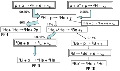
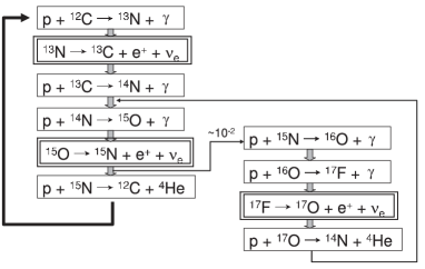
Figure 1: $pp$ chain and CNO cycle reactions

In the figure, the reactions marked with double borders produce neutrinos, and the neutrinos from these reactions are named depending on the reaction: $pp$, ${}^{7}{\rm Be}$, ${}^{8}{\rm B}$, $hep$, ${}^{13}{\rm N}$, ${}^{15}{\rm O}$ and ${}^{17}{\rm F}$ neutrinos. The fluxes of each neutrino type from the latest SSMSSM2017 are shown in Table 1.

source	flux (/cm2/s)
	GS98	AGSS09met
$pp$	5.98 $\times 10^{10}(1\pm 0.006)$	6.03 $\times 10^{10}(1\pm 0.005)$
${}^{7}{\rm Be}$	4.93$\times 10^{9}(1\pm 0.06)$	4.50$\times 10^{9}(1\pm 0.06)$
$pep$	1.44$\times 10^{8}(1\pm 0.01)$	1.46$\times 10^{8}(1\pm 0.009)$
${}^{8}{\rm B}$	5.46$\times 10^{6}(1\pm 0.12)$	4.50$\times 10^{6}(1\pm 0.12)$
$hep$	7.98$\times 10^{3}(1\pm 0.30)$	8.25$\times 10^{3}(1\pm 0.30)$
${}^{13}{\rm N}$	2.78$\times 10^{8}(1\pm 0.15)$	2.04$\times 10^{8}(1\pm 0.14)$
${}^{15}{\rm O}$	2.05$\times 10^{8}(1\pm 0.17)$	1.44$\times 10^{8}(1\pm 0.16)$
${}^{17}{\rm F}$	5.29$\times 10^{6}(1\pm 0.20)$	3.26$\times 10^{6}(1\pm 0.18)$

Table 1: Solar neutrino flux predicted by SSMSSM2017 . The second and third columns show the flux predictions using the chemical composition from GS98GS98 and AGSS09metAGSS09 , respectively.

The second and third columns in the table show the flux predictions using chemical compositions obtained by GS98GS98 and AGSS09metAGSS09 , respectively. GS98 is based on a one-dimensional model of the solar atmosphere that was released in 1998. AGSS09met, released in 2009, is based on a three-dimensional model and uses the most up-to-date atomic and molecular data, and should therefore be more reliable than the GS98-based solar model. However, the GS98-based solar model can reproduce various observations inside the sun, such as the sound speed profile, depth of the convective zone and the helium abundance, while the AGSS09met based solar model’s predictions have large discrepancies with observations. Therefore, the flux predictions of both are given here.

The energy spectrum of solar neutrinos predicted by the SSM is shown in Fig.2.

Figure 2: Solar neutrino energy spectrum expected from the SSMSOLBP2001 ; SOLBP2004 . The solid and dashed curves show neutrinos in the $pp$ chain and CNO cycle, respectively.

The most energetic neutrino is the ⁸B neutrino and it was the main neutrino source for the Homestake, Kamiokande, Super-Kamiokande and SNO experiments, though its intensity is only about 0.01% of the total solar neutrino flux. The most abundant source is the $pp$ neutrino but its maximum energy is only 0.42 MeV. The gallium experiments were sensitive to $pp$ neutrinos.

3 Homestake experiment

The Homestake experiment was located in the Homestake gold mine at a depth of 1480 metersSOLDAVIS . The experiment was started around 1970 and data were obtained until 1994. The target for the solar neutrinos was ${}^{37}{\rm Cl}$ atoms in 615 tons of ${\rm C}_{2}{\rm Cl}_{4}$. The neutrino energy threshold of the reaction ${}^{37}{\rm Cl}+\nu_{e}\rightarrow^{37}{\rm Ar}+e^{-}$ is 0.814 MeV and it is mainly sensitive to ⁸B neutrinos. This radiochemical Cl-Ar method of solar neutrino detection was proposed by B. Pontecorvo in 1946PONT1946 . The expected event rate from the SSMSOLBP2004 was 8.5$\pm$1.8 SNU, where one SNU is $10^{-36}$captures/atom/s. The contribution from each neutrino source is 6.6 SNU from ${}^{8}{\rm B}$ neutrinos, 1.2 SNU from ⁷Be neutrinos, 0.22 SNU from $pep$ neutrinos and the remainder from CNO cycle neutrinos. The produced ${}^{37}{\rm Ar}$ atoms were collected once every 60–120 days and the decay of ${}^{37}{\rm Ar}$ was counted using a low background proportional counter. Figure 3 shows the observed production rate of ${}^{37}{\rm Ar}$ in each collection cycleSOLDAVIS .

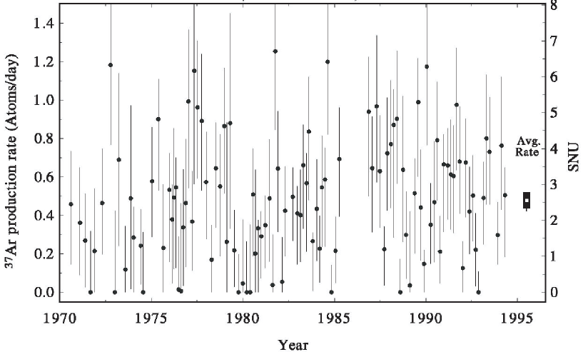
Figure 3: Data from the Homestake experimentSOLDAVIS . Each data point shows the ${}^{37}{\rm Ar}$ production rate measured in each collection cycle (run). The scale of the right hand side is in SNU. The time averaged rate is shown to the right of the main data.

The average event rate observed by the Homestake experiment was

$$\phi(Homestake)=2.56\pm 0.16(stat.)\pm 0.16(sys.)~{}~{}{\rm SNU}$$

The observed event rate was only about 30% of the SSM prediction, leading to the so-called solar neutrino problem.

4 Kamiokande

The Kamiokande detector was constructed in 1983 to search for proton decay. The detector had a 2340 ton water volume, located 1000 meters underground in the Kamioka Mine in Japan. The water volume was viewed by 1,000 20-inch diameter photomultipliers (PMTs) mounted on a 1-m grid on the inner surface. Data collection was started on July 6, 1983 and tens of proton decay events within a few months were expected if the original idea of the grand unified theoryGGGUT is correct. However, no proton decay events were found. Since the primary purpose of the detector was to observe events with $\sim$1 GeV total energy, low-energy events such as solar neutrinos were not triggered in the first stage of the Kamiokande experiment as the electronics at that time read out only the integrated charge information for each PMT. The total sum signal, which is the sum of analog signals from all PMTs, was used to trigger the readout electronics, and the trigger energy threshold was about 30 MeV for electrons, which is much higher than the energy of solar neutrino signals. The total sum signal was recorded by a transient digitizer (R7912, Tektronix), which records a digitized oscilloscope image in order to detect $\mu\rightarrow e$ decay signals from stopping muons. There were several hundred cosmic ray stopping muons per day in the Kamiokande detector. Figure 4 shows the pulse height distribution of $\mu\rightarrow e$ signals.

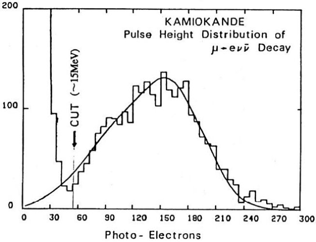
Figure 4: Pulse height distribution of $\mu\rightarrow e$ signals of stopping cosmic ray muons at the early stage of Kamiokande.

The distribution showed that the Kamioka detector had the potential to detect low-energy neutrinos down to $\sim$10 MeV, and Prof. Koshiba proposed upgrading the detector for ${}^{8}{\rm B}$ solar neutrino measurements in the fall of 1983.

In order to detect solar neutrinos, two major upgrades were required. First, an anti-counter system had to be constructed to reduce environmental background signals such as gamma rays from radioactivity in the surrounding rock. Second, a new set of electronics to read out the timing and charge information of each individual PMT was necessary. Precise determination of the position where an event occurred, called the vertex position, is crucial for solar neutrino measurements. The gamma rays from the rock which remained after passing through the anti-counter tended to have a vertex position near the wall of the detector. High-energy cosmic rays produce hadronic cascade showers by spallation and generate short-life radioactive nuclei. The event rate of the beta decays of those nuclei was more than one order of magnitude higher than the expected rate of ${}^{8}{\rm B}$ solar neutrino signals. Those spallation products were produced along the track of the originating cosmic ray muons and could be removed using the vertex information.

The anti-counter was constructed from September 1984 through March 1985. 123 20-inch PMTs were mounted in the anti-counter to work as an active veto. The bottom PMT plane of the inner-counter was lifted by 1.2 m to allow PMTs to be inserted for the bottom anti-counter. The PMTs for the top anti-counter were mounted 0.8 m above the top inner-counter. Additional water was added to the tank to submerge these PMTs. The Kamiokande tank was constructed in a newly excavated cavern, and rubber-asphalt was sprayed on the surface of the cavern to make it water-tight so that water could be filled between the cavern wall and the Kamiokande tank. PMTs were mounted in this newly prepared layer, which functioned as the barrel part of the anti-counter. A schematic view of the Kamiokande detector after the upgrade is shown in Fig.5.

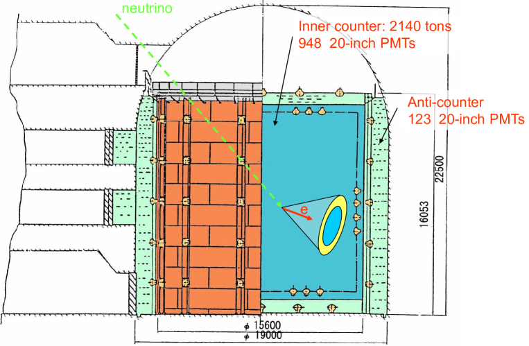
Figure 5: Schematic view of the Kamiokande detector after the upgrade.

Prof. Koshiba gave a talk on the possibility of detecting ${}^{8}{\rm B}$ solar neutrinos in Kamiokande at ICOBAN’84 (International Conference On BAryon Non-conservation, Park City, Utah, 1984) and asked the participants to collaborate on the electronics upgrade. Soon after this workshop, the Univ. Pennsylvania group led by Prof. A.K. Mann expressed interest in producing the new electronics. The electronics system, included timing and charge readouts and a trigger system using number-of-hit PMTs, was installed in the fall of 1985.

A further consideration was radon in the tank water, which is the most significant source of background noise in solar neutrino measurements. The concentration of radon, especially ${}^{222}{\rm Rn}$, was two or more orders of magnitude higher in the air and water in the mine than in the usual environment outside the mine. A daughter of ${}^{222}{\rm Rn}$, ${}^{214}{\rm Bi}$, emits beta rays with an end-point energy of 3.27 MeV, which mimics a solar neutrino signal. When Kamiokande started collecting data after the installation of anti-counters, fresh water was being constantly supplied to the tank. The trigger rate in the lower energy threshold mode was several hundred events per second, while the goal was at most only about one solar neutrino event per day. Figure 6 shows the change in trigger rate after a modification was made to recirculate water rather than supplying fresh water. The decrease in the trigger rate was consistent with the decay of ${}^{222}{\rm Rn}$ with a half life of 3.8 days.

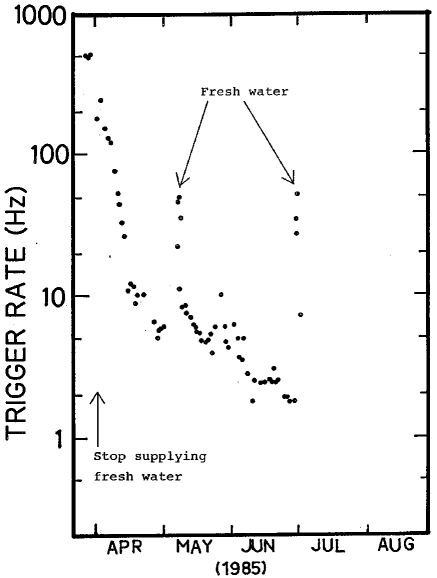
Figure 6: Change in trigger rate after changing to recirculated water without supplying fresh water.

Various efforts were made to further reduce radon in the tank water in 1986, including air-tightening of buffer tanks in the water purification system. The detector was almost ready for solar neutrino measurements in early 1987.

Prof. Koshiba noted that the following three features are necessary to perform “neutrino astronomy”:

• Directionality

• Real-time measurement

• Energy spectrum measurement

In Kamiokande, solar neutrino signals were observed based on the Cherenkov radiation of recoil electrons from neutrino–electron scattering. Since the energy of ${}^{8}{\rm B}$ solar neutrino is much larger than the mass of an electron, the direction of a scattered electron is strongly correlated with the direction from the sun to the earth. In addition, since Kamiokande observed images of the Cherenkov ring pattern, the direction of the electron could be observed. Kamiokande was a real-time detector and events were observed at the time when they happened. The energy spectrum of the neutrinos could be deduced from the spectrum of the scattered electrons. Thus, the observations at Kamiokande satisfied the criteria for neutrino astronomy.

Figure 7 shows the angular distribution to the sun for the events that passed the criteria for solar neutrino event selection. The plot was obtained with initial 450-day data taken from January 1987 to May 1988SOLKAMIOKANDE1 .

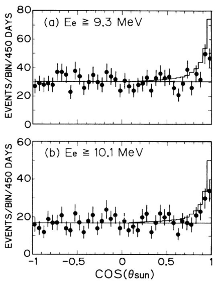
Figure 7: Angular distribution to the direction of the sun in KamiokandeSOLKAMIOKANDE1 . The plot shows data from the first 450 days of data taken from January 1987 to May 1988. The solid histogram shows the prediction from the SSM.

A clear excess of events was observed in the direction of the sun but the observed rate was about 50% of the prediction from the SSM (solid histogram in the figure). This observation confirmed the solar neutrino problem.

The Kamiokande detector observed $\sim$600 solar neutrino events by February 1995SOLKAMIOKANDE2 and the obtained flux of ⁸B neutrino was

$$\phi(^{8}{\rm B})_{Kamiokande} = 2.80\pm 0.19(\mbox{stat.})\pm 0.33(\mbox{sys.})$$

$$\times 10^{6}/cm^{2}/s~{}.$$

The observed flux was 48$\pm$3(stat.)$\pm$6(sys.) % of the prediction from the SSM. The energy spectrum of recoil electrons normalized by the predicted spectrum is shown in Fig.8,

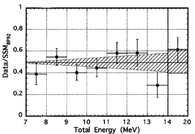
Figure 8: Energy spectrum of recoil electrons normalized by the predicted spectrum from the 2079-day dataset of Kamiokande. The hatched area shows the range of systematic uncertainty.

consistent with a flat spectrum, i.e. no hint of neutrino oscillations was given in the spectrum. In order to proceed to investigate possibility of neutrino oscillations, high statistics measurements with Super-Kamiokande was necessary.

5 Status just before the start of Super-Kamiokande and SNO

This section describes other experiments that have been performed and how we enhanced our understanding of the solar neutrino problem before the Super-Kamioakande/SNO era.

SAGE and GALLEX were radiochemical experiments using gallium targets conducted since the early 1990s. The SAGE experimentSAGE1994 ; SAGE2001 ; SAGE2009 was conducted at the Baksan Observatory and the GALLEX experiment GALLEX94 ; GALLEX95 ; GALLEX96 (later changed to GNOSOLGNO ) was conducted at the Gran Sasso Laboratory. The energy threshold of the gallium reaction (${}^{71}{\rm Ga}+\nu_{e}\rightarrow^{71}{\rm Ge}+e^{-}$) is 0.233 MeV and is mainly sensitive to low-energy solar neutrinos. The expected event rate from the SSMSOLBP2004 is 131${}^{+12}_{-10}$ SNU, with contributions of 69.6 SNU from $pp$ neutrinos, 34.8 SNU from ⁷Be neutrinos, 13.9 SNU from ${}^{8}{\rm B}$ neutrinos, 2.9 SNU from $pep$ neutrinos and the remainder from CNO cycle neutrinos. SAGE used 50 tons of gallium in metallic form and GALLEX/GNO used 30 tons of gallium in a GaCl${}_{3}\cdot$HCl solution. The lifetime of ⁷¹Ge is 16.5 days and a typical exposure time for one run was 28 days. By the middle of 1990s, a deficit of solar neutrinos had been observed at SAGE and GALLEX, where the predicted event rate was mainly coming from robust sources such as $pp$ and ⁷Be neutrinos. The final results of the gallium experiments are shown here but the conclusion had not been changed since the middle of the 1990s. The average event rates observed by SAGE and GALLEX/GNO were

$$\phi(SAGE)=65.4^{+3.1}_{-3.0}(stat.)^{+2.6}_{-2.8}(sys.)~{}{\rm SNU}$$

$$\phi(GALLEX)=73.1^{+6.1}_{-6.0}(stat.)^{+3.7}_{-4.1}(sys.)~{}{\rm SNU}$$

$$\phi(GNO)=62.9^{+5.5}_{-5.3}(stat.)^{+2.5}_{-2.5}(sys.)~{}{\rm SNU}~{}.$$

Combining these resultsSAGE2009 , the flux measured by the gallium experiments was

$$\phi(gallium)=66.1\pm 3.1~{}~{}{\rm SNU}$$

The observed flux is 50% of the expectation from the SSMSOLBP2004 .

Since it was difficult to attribute the deficits of the neutrino event rates at the Homestake, Kamiokande and SAGE/GALLEX experiments to potential problems in the SSM, the possibility of solar neutrino oscillations was extensively discussed in the mid 1990s. Assuming two types of neutrinos, the relation between the mass eigenstates of the two neutrinos ($\nu_{1}$ and $\nu_{2}$) and their interaction eigenstates($\nu_{e}$ and $\nu_{X}$(X=$\mu,\tau$)) is expressed as

$$\left(\begin{array}[]{c}\nu_{e}\\ \nu_{X}\\ \end{array}\right) = \left(\begin{array}[]{cc}\cos\theta&\sin\theta\\ -\sin\theta&\cos\theta\\ \end{array}\right)\left(\begin{array}[]{c}\nu_{1}\\ \nu_{2}\\ \end{array}\right)~{},$$ (7)

where $\theta$ is the mixing angle. Solving the time evolution of the neutrino wave function, the probability that produced as electron-type neutrinos are observed as eletron-type neutrinos is

$$P(\nu_{e}\rightarrow\nu_{e}) = 1-\sin^{2}2\theta\times\sin^{2}\left(1.27\times\Delta m^{2}\frac{L}{E}\right)~{},$$

where $\Delta m^{2}$ is the mass squared difference ($m_{2}^{2}-m_{1}^{2}$) in units of eV², $L$ is the neutrino travel length in meters, and $E$ is neutrino energy in MeV. If the argument of the last sine function, $1.27\times\Delta m^{2}\frac{L}{E}$, is much larger than $2\pi$, it averages out and the survival probability becomes :

$$P(\nu_{e}\rightarrow\nu_{e}) = 1-{1\over 2}\sin^{2}2\theta~{}.$$

In the case of solar neutrino oscillation, the effect of matter in the sun and the earth must be considered. The matter effect was originally discussed by L. WolfensterinSOLMSWW in 1978. P. Langacker, J. P. Leveille and J. Sheiman corrected a sign mistake in the Wolfensterin’s paper in 1983LLS1983 . Then in 1985, S. P. Mikheyev and A. Y. Smirnov pointed out that the significant deficit of the event rate in Homestake, especially much less than the half of the expectation, can be explained by the matter effectSOLMSWMS . As you can see in the upper equation, the $P(\nu_{e}\rightarrow\nu_{e})$ cannot be less than 0.5, but the matter effect can make it much less than 0.5 if $\Delta m^{2}>0$, i.e. $m_{2}>m_{1}$. Thus, the mass ordering of $m_{2}$ and $m_{1}$ was determined by the solar neutrino observations. In 1993, global analyses had been performedKRAPET1993 ; HATALANG1993 and a typical contour plot of the oscillation parameters at that time is shown in Fig.9.

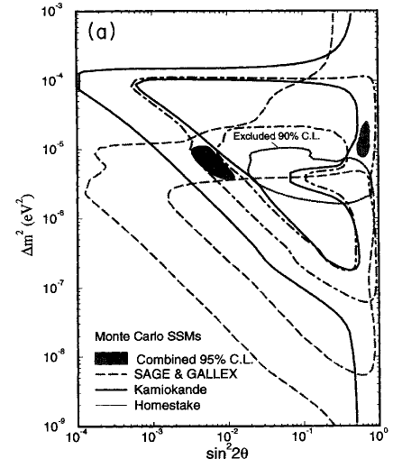
Figure 9: Global analysis performed by Hata and Langacker in 1993HATALANG1993 .

The two solutions shown in the figure are called the SMA (small mixing angle) and LMA (large mixing angle) solutions for $\sin^{2}2\theta\sim 10^{-2}$ and $\sin^{2}2\theta\sim 0.6$, respectively.

To obtain information about neutrino oscillations, it was necessary to measure something that is independent of solar models. Possibilities were the shape of the energy spectrum and the time variation of solar neutrino event rates, such as the day/night difference. Another possibility, which is more robust, was a comparison between event rates measured with charged current and neutral current interactions, which are sensitive to only ${\nu}_{\rm e}$ and all neutrino types, respectively. Regarding the shape of the energy spectrum and the day/night difference, Fig.10 shows the neutrino survival probability as a function of energy for each solution.

Super-Kamiokande aimed to measure the energy spectrum shape distortion, which is expected for SMA, and the day/night difference, which is expected for LMA with smaller $\Delta m^{2}$. As will be described in Section 9, the first model-independent discovery of neutrino oscillations was in a comparison between a charged current measurement by SNO (i.e. ${\nu}_{\rm e}$ flux measurement) and an electron-scattering measurement by Super-Kamiokande (which had contributions from $\nu_{\rm\mu}$ and ${\nu}_{\rm\tau}$).

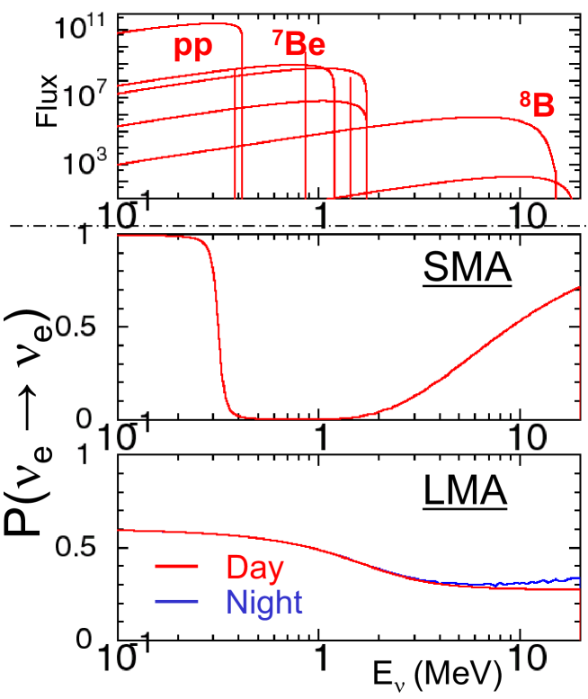
Figure 10: Neutrino survival probability as a function of energy for typical oscillation parameters in each solution. The top plot is the predicted solar neutrino spectrum from the SSM.

6 Super-Kamiokande

The Super-Kamiokande (SK) detector is a 50,000-ton water Cherenkov detector located 1000 meters underground in the Kamioka Mine in Japan. Yoji Totsuka led the detector construction and initial analyses of SK data. The detector has an inner active volume (32,000 tons) viewed by 11,146 20-inch diameter photomultipliers (PMTs). The fiducial volume for the solar neutrino measurement is 22,500 tons, defined by the volume more than 2 m from the surface of the PMTs. A schematic view of the SK detector is shown in Fig.11.

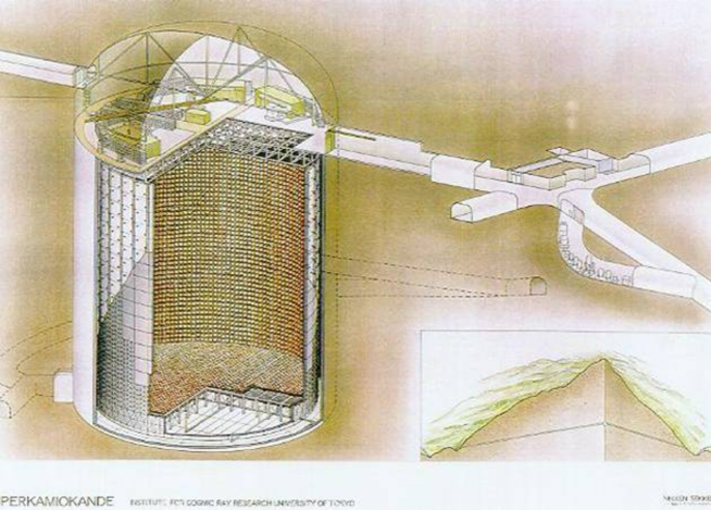
Figure 11: Schematic view of the Super-Kamiokande detector.

SK has measured ${}^{8}{\rm B}$ neutrinos using neutrino–electron scattering in the same manner as Kamiokande. The main difference between Super-Kamiokande and Kamiokande is the 30 times larger fiducial volume and increased fraction of photo-sensitive coverage by a factor of 2, which enabled the energy threshold to be lowered below 5 MeV.

To measure the ${}^{8}{\rm B}$ solar neutrino flux energy spectrum with high precision, special care was taken in SK. The absolute energy of the detector was calibrated using an electron linear accelerator (LINAC)LINACPAP installed at the detector site. The LINAC system could generate mono-energetic electrons and inject them at various positions in the detector. The LINAC system provided a very precise energy scale calibration, but it is only accurate for vertical downward-going events. To calibrate the angular dependence of the energy scale, a ¹⁶N radioactive sourceSKN16 was used. ¹⁶N atoms are produced by fast neutron capture by oxygen nuclei in water. Neutrons were generated by a commercially built deuteron–tritium generator which produced 10⁶ 14.2-MeV neutrons per pulse. The main decay mode of ¹⁶N is an electron with a 4.3-MeV maximum energy coincident with a 6.1-MeV gamma ray. A setup of the DT generator was deployed in the SK tank, and it is raised by about 2 m after it emits neutrons in order to avoid shadowing of the Cherenkov light. Because of the precise energy calibration by the LINAC and DT systems, the absolute energy scale of the SK detector was calibrated with an accuracy of 0.64% (rms) in the first phase of the SK detector (SK-I) and was improved to 0.53 % in the fourth phase.

SK-I ran for 1496 live-days from May 1996 to July 2001SOLSK2001 ; SOLSKFULL ; SOLSK2002 . In November 2001, a chain reaction implosion destroyed more than half of the PMTs, such that the second phase (SK-II) ran for 791 live-days from December 2002 to October 2005, using 5,182 ID PMTs with 19% photocathode coverageSOLSK2008 . Since SK-II the ID PMTs have been covered in fiber-reinforced plastic cases with an acrylic window to prevent similar accidents. The detector was fully reconstructed from October 2005 to July 2006 and the third phase (SK-III) ran for 548 live-days from October 2006 to August 2008SOLSK2010 . The readout electronics were replaced in September 2008 and the fourth phase (SK-IV) ran for 2970 live-days until May 2018SOLSK2020 . The SK tank was refurbished to make it leak-tight for a future upgrade (as explained later) from June 2018 to January 2019. The fifth phase (SK-V) ran from February 2019 through June 2020 with pure water. 13 tons of Gd₂(SO₄)${}_{3}\cdot$H₂O was loaded into the tank water to make a 0.01 %wt Gd solution from July to August in 2020 and the sixth phase (SK-VI) is running with a neutron tagging capability. Solar neutrino data analyses were performed for all SK phases and were completed by SK-IV. Figure 12 shows the angular distribution of solar neutrino candidates with respect to the direction of the sun from SK-IV. Solar neutrino events are clearly seen above the flat background distribution.

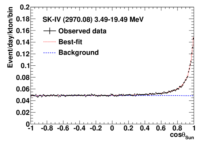
Figure 12: Angular distribution with respect to the direction of the sun in Super-Kamiokande phase IVSOLSK2020 .

Table 2 shows live-times, energy thresholds, measured fluxes, ratios compared with a Monte Carlo simulation (in which ${}^{8}{\rm B}$ flux of 5.25$\times 10^{6}$/cm²/s is assumed) and the numbers of extracted signals for each SK phase, and combined results.

Phase	Livetime	Threshold	Measured Flux	DATA/MC	# of signals
	(days)	(MeV)	($10^{6}$/cm2/s)		($\pm$stat. only)
SK-I	1496	4.5	2.38$\pm 0.02\pm 0.08$	0.453$\pm 0.005^{+0.016}_{-0.014}$	22443${}^{+227}_{-225}$
SK-II	791	6.5	2.41$\pm 0.05^{+0.16}_{-0.15}$	0.459$\pm 0.010\pm 0.030$	7210${}^{+153}_{-151}$
SK-III	548	4.0	2.40$\pm 0.04\pm 0.05$	0.458$\pm 0.007\pm 0.010$	8148$\pm 133$
SK-IV	2970	3.5	2.33$\pm 0.01\pm 0.03$	0.443$\pm 0.003\pm 0.006$	63890${}^{+381}_{-379}$
Combined	5805	-	2.35$\pm 0.01\pm 0.04$	0.447$\pm 0.002\pm 0.008$	More than
					100k events

Table 2: Summary of flux measurements at Super-Kamiokande.

The energy threshold of the data analysis was 4.5 MeV (kinetic energy) in SK-I but was lowered to 3.5 MeV in SK-IV. That was possible because the radon background in the tank water was reduced by a stable laminar flow in the tank given by a precise temperature control.

In addition, the systematic error was reduced by more precise calibrations and detailed studies of the efficiencies of various cuts. When SK started data collection in 1996, the solar activity was near the minimum. The SK data covered almost two solar cycles until the end of SK-IV. Figure 13 shows the measured yearly fluxes compared with the solar activity. The measured fluxes are consistent with a flat distribution within statistical and systematic errors and no correlation with the solar activity was observed.

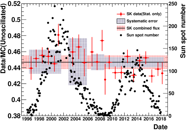
Figure 13: Yearly plot of the ${}^{8}{\rm B}$ solar neutrino flux measured by SK, shown as red points with error bars. The black dots show the number of sunspots, from SUNSPOT .

The energy spectrum shape is important for the discussion of neutrino oscillations. Figure 14 shows energy spectra of solar neutrino signals observed in each SK phase compared with the expected spectrum without neutrino oscillations. A ${}^{8}{\rm B}$ flux of 5.25$\times 10^{6}$/cm²/s is assumed in this figure, based on the SNO neutral current measurement, consistent with the SSM predictions.

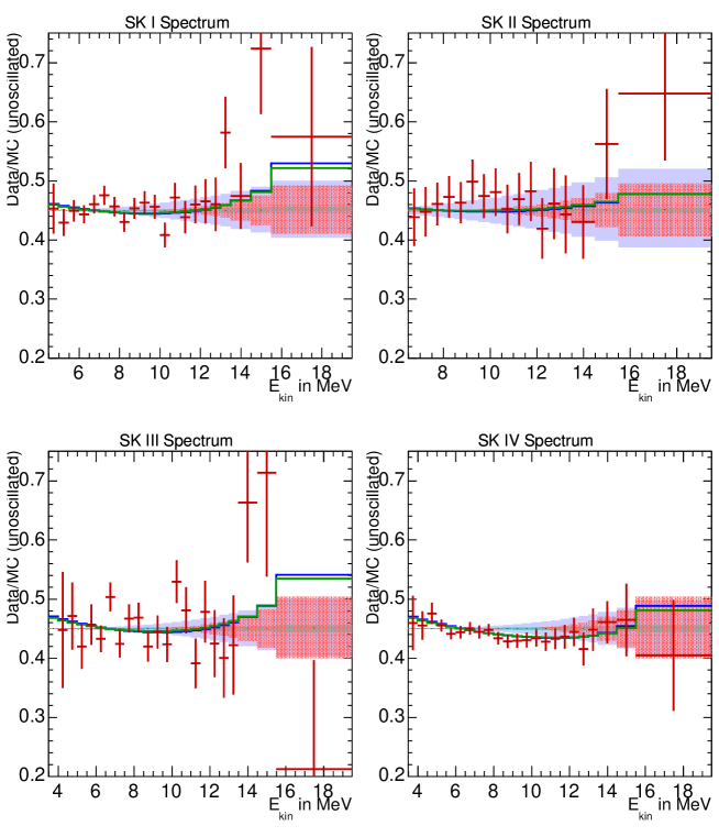
Figure 14: Energy spectrum of the solar neutrino signal observed in each SK phase. The vertical axis is normalized by the spectrum without neutrino oscillations with a flux of 5.25$\times 10^{6}$/cm²/s. The blue and green histograms show the expectations with neutrino oscillations with parameters from the KamLAND reactor measurementKAMLAND and solar global analysis, respectively. The bands around the horizontal line show $\pm 1\sigma$ energy-correlated systematic errors.

The observed energy spectrum shapes in SK-I, II and III are consistent with a flat oscillation probability. The SK-IV spectrum shape disfavors a flat probability with a significance of $\sim 1\sigma$, which is consistent with the shape expected from the oscillation parameters obtained by the KamLAND reactor measurementKAMLAND .

The day/night flux difference was evaluated by an asymmetry parameter ($A_{DN}$) defined as $\frac{(day-night)}{\frac{1}{2}(day+night)}$. The asymmetry parameters measured by SK-ISOLSK2002 , SK-IISOLSK2008 , SK-IIISOLSK2010 and SK-IVSOLSK2020 were

$$A^{SK-I}_{DN} = -0.021\pm 0.020\mbox{(stat.)}^{+0.013}_{-0.012}\mbox{(sys.)}$$

$$A^{SK-II}_{DN} = -0.063\pm 0.042\mbox{(stat.)}\pm 0.037\mbox{(sys.)}$$

$$A^{SK-III}_{DN} = -0.056\pm 0.031\mbox{(stat.)}\pm 0.013\mbox{(sys.)}$$

$$A^{SK-IV}_{DN} = -0.021\pm 0.011\mbox{(stat.)}\hskip 28.45274pt\mbox{(preliminary)}$$

Since $A_{DN}$ depends on $\Delta m^{2}$, as shown by the red curve in Fig.15, we can measure $\Delta m^{2}$ by $A_{DN}$. This is a unique method for measuring $\Delta m^{2}$ using solar neutrinos and is likely to be the only method for neutrinos. (Note that $\Delta m^{2}$ can be measured for anti-neutrinos using reactor neutrinos.) To demonstrate the accuracy of the $\Delta m^{2}$ measurement, $A_{DN}$ for SK-IV is shown in Fig.15 by black data points with statistical errors.

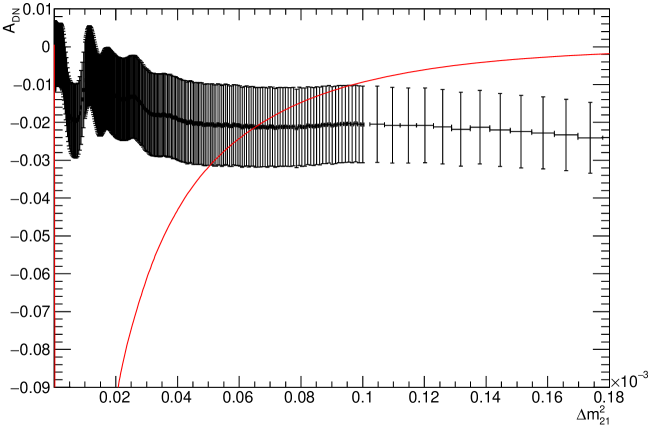
Figure 15: Expected asymmetry from matter oscillation in the earth as a function of $\Delta m^{2}_{21}$ (red curve) and SK-IV data with its statistical error (black data points).

7 SNO

The Sudbury Neutrino Observatory (SNO) detector was a 1000-ton heavy water (D₂O) Cherenkov detector located 2090 meters underground in the Creighton Mine near Sudbury, Canada. It used 9456 8-inch diameter PMTs to view heavy water contained in an acrylic vessel. The SNO detector could measure the $\nu_{e}$ flux from ⁸B neutrinos and the flux of all active neutrino flavors through the following interactions:

$$\begin{array}[]{lcll}\nu_{e}+d&\rightarrow&p+p+e^{-}&\hskip 3.61371pt\mbox{(charged current (CC))}\\ \nu_{x}+d&\rightarrow&p+n+\nu_{x}&\hskip 3.61371pt\mbox{(neutral current (NC))}\\ \nu_{x}+e^{-}&\rightarrow&\nu_{x}+e^{-}&\hskip 3.61371pt\mbox{(electron scattering (ES))}\\ \end{array}$$

where $\nu_{x}$ is any of $\nu_{e}$, $\nu_{\mu}$ or $\nu_{\tau}$. The first phase of SNO data collection (SNO-I) was undertaken using a pure D₂O target over 306 days from November 1999 to May 2001SOLSNO1 . Free neutrons from the NC interaction were thermalized and 6.25-MeV $\gamma$ rays were emitted following their capture by deuterons. The capture efficiency was about 30%. The measured fluxes were

$$\phi(^{8}{\rm B})^{CC}_{SNO-I} = 1.76\pm 0.05\mbox{(stat.)}\pm 0.09\mbox{(sys.)}\times 10^{6}/cm^{2}/s$$

$$\phi(^{8}{\rm B})^{ES}_{SNO-I} = 2.39^{+0.24}_{-0.23}\mbox{(stat.)}\pm 0.12\mbox{(sys.)}.\times 10^{6}/cm^{2}/s$$

$$\phi(^{8}{\rm B})^{NC}_{SNO-I} = 5.09^{+0.44}_{-0.43}\mbox{(stat.)}^{+0.46}_{-0.43}\mbox{(sys.)}\times 10^{6}/cm^{2}/s~{}.$$

In the second phase of the SNO experiment (SNO-II), 2 tons of NaCl were added to the D₂O target to enhance the detection efficiency of the NC channelSOLSNO2 . Thermalized neutrons were captured by ³⁵Cl nuclei, resulting in the emission of a $\gamma$-ray cascade with a total energy of 8.6 MeV. The CC and NC signals were statistically separated using the isotropy of the Cherenkov light pattern and each event’s angle to the sun. The forward peaked signal was due to ES and the backward distribution was due to CC interactions. NC events were isotropic with respect to the solar direction. The measured fluxes in SNO-II were

$$\phi(^{8}{\rm B})^{CC}_{SNO-II} = 1.68\pm 0.06\mbox{(stat.)}^{+0.08}_{-0.09}\mbox{(sys.)}\times 10^{6}/cm^{2}/s$$

$$\phi(^{8}{\rm B})^{ES}_{SNO-II} = 2.35\pm 0.22\mbox{(stat.)}^{+0.15}_{-0.15}\mbox{(sys.)}\times 10^{6}/cm^{2}/s$$

$$\phi(^{8}{\rm B})^{NC}_{SNO-II} = 4.94\pm 0.21\mbox{(stat.)}^{+0.38}_{-0.34}\mbox{(sys.)}\times 10^{6}/cm^{2}/s.$$

In the third phase of SNO (SNO-III), ³He proportional counters were deployed in the heavy water and the NC events were measured independentlySOLSNO3 . The NC flux measured by SNO-III was

$$\phi(^{8}{\rm B})^{NC}_{SNO-III} = 5.54^{+0.33}_{-0.31}\mbox{(stat.)}^{+0.36}_{-0.34}\mbox{(sys.)}\times 10^{6}/cm^{2}/s.$$

The SNO group performed a combined analysisSOLSNOCOMB of all three phases and the obtained result was

$$\phi(^{8}{\rm B})^{NC}_{SNO~{}combined} = 5.25\pm 0.16\mbox{(stat.)}^{+0.11}_{-0.13}\mbox{(sys.)}\times 10^{6}/cm^{2}/s.$$

Compared with the ${}^{8}{\rm B}$ flux value in Table 1, the observed ${}^{8}{\rm B}$ flux with NC by SNO agrees well with the prediction within the errors. Combining the statistical and systematic errors, the total error of the flux observed by SNO is 3.8%, which is better than that of the SSM prediction by a factor of 3. Therefore, the SNO value was used to make plots of SK in the previous section and will be used in the discussion of the global oscillation analysis in Section 9.

8 Borexino

Borexino is a liquid scintillator detector with an active mass of 278 tons of pseudocumene located in the Gran Sasso Laboratory. Scintillation light is detected via 2212 8-inch PMTs uniformly distributed on the inner surface of the detector. Because of the high light yield of a liquid scintillator compared with Cherenkov light, Borexino is sensitive to sub-MeV solar neutrinos. The first ⁷Be solar neutrino measurement was reported in Borexino-1st , based on 192 days of data taken from May 2007 to April 2008. The 0.862-MeV monoenergetic ⁷Be neutrinos were detected by neutrino–electron scattering. The energy spectrum of observed events was deconvoluted using the expected shape of the recoil electrons and possible background sources. Thus, the extracted ⁷Be neutrino event rate was

$$49\pm 3\mbox{(stat.)}\pm 4\mbox{(sys.)}~{}{\rm counts}/({\rm day}\cdot 100{\rm ton)},$$

while the expected event rate from the SSM was $74\pm 4~{}{\rm counts}/({\rm day}\cdot 100{\rm ton})$. The deficit of the observed ⁷Be neutrino event rate is consistent with the expectation based on neutrino oscillations. Borexino also succeeded in observing $pep$, $pp$ and CNO solar neutrinos, reported in Borexino-pep , Borexino-pp and Borexino-CNO , respectively. The Borexino group corrected the effect of neutrino oscillations and obtained fluxes of $pp$, ⁷Be, $pep$ and CNO neutrinos from the second phase of Borexino asBorexino2 ; Borexino-CNO

$$\phi(pp)^{Osc.corrected}_{Borexino} = 6.1\pm 0.5\mbox{(stat.)}^{+0.3}_{-0.5}\mbox{(sys.)}\times 10^{10}/cm^{2}/s$$

$$\phi(^{7}{\rm Be})^{Osc.corrected}_{Borexino} = 4.99\pm 0.11\mbox{(stat.)}^{+0.06}_{-0.08}\mbox{(sys.)}\times 10^{9}/cm^{2}/s$$

$$\phi(pep(HZ/LZ))^{Osc.corrected}_{Borexino} = 1.27/1.39\pm 0.19\mbox{(stat.)}^{+0.08}_{-0.12/-0.13}\mbox{(sys.)}\times 10^{8}/cm^{2}/s$$

$$\phi({\rm CNO})^{Osc.corrected}_{Borexino} = 7.0^{+3.0}_{-2.0}\mbox{(sys.)}\times 10^{8}/cm^{2}/s$$

These fluxes are compared with the SSM predictions in Table 1 and are consistent with each other within the experimental errors.

9 Solar Neutrino Oscillations

Precise solar neutrino measurements have shown that the solar neutrino problem is due to neutrino oscillations. In this section, a brief history of and the latest results for solar neutrino oscillations are discussed.

9.1 Evidence of solar neutrino oscillations

In March 2001, the SK collaboration released results of the precise measurement of the ${}^{8}{\rm B}$ flux using 1258 days of SK dataSOLSK2001 . SK measured ${}^{8}{\rm B}$ solar neutrinos using neutrino–electron scattering (ES), in which $\nu_{\rm\mu}$ and ${\nu}_{\rm\tau}$ contribute in addition to ${\nu}_{\rm e}$ because the cross section of $\nu_{\nu/\tau}e^{-}$ scattering is about 1/($6\sim 7$) of that for $\nu_{e}e^{-}$ scattering. In June 2001, the SNO collaboration released the first result of the charged current (CC), i.e. ${\nu}_{\rm e}$, measurement, including the plot in Fig.16, which demonstrated that $\nu_{\mu/\tau}$ exist with more than 3$\sigma$ significanceSNOfirstCC . That was the first direct evidence for solar neutrino oscillations.

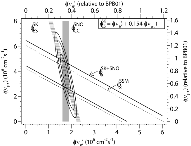
Figure 16: ${\nu}_{\rm e}$ flux and $\nu_{\mu/\tau}$ flux contour obtained from the results of SK and SNO in 2001SNOfirstCC . Each band shows the $\pm 1\sigma$ range of each measurement.

The SNO collaboration published NC current measurements, the results of which were described above in section 7. The SK collaboration provided further data for analysis and improved the accuracy of the ES measurement. The plot in Fig.17 uses the latest data from SK and SNO, including NC data, showing that the significance of $\nu_{\mu/\tau}$ had been greatly improved. The measurements of SK and SNO are consistent with each other.

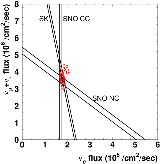
Figure 17: Latest ${\nu}_{\rm e}$ flux and $\nu_{\mu/\tau}$ flux contour obtained from the results of SKSOLSK2020 and SNOSOLSNO1 ; SOLSNO2 ; SOLSNO3 ; SOLSNOCOMB . Each band shows the $\pm 1\sigma$ range for each measurement.

9.2 Determination of oscillation parameters

In the three flavor neutrino framework, the relation between the mass and interaction eigenstates is described by

$$\left(\begin{array}[]{c}{\nu}_{\rm e}\\ \nu_{\rm\mu}\\ {\nu}_{\rm\tau}\\ \end{array}\right) = \left(\begin{array}[]{ccc}U_{e1}&U_{e2}&U_{e3}\\ U_{\mu 1}&U_{\mu 2}&U_{\mu 3}\\ U_{\tau 1}&U_{\tau 2}&U_{\tau 3}\\ \end{array}\right)\left(\begin{array}[]{c}\nu_{1}\\ \nu_{2}\\ \nu_{3}\\ \end{array}\right)$$ (17)

The unitary matrix $U$ is the Pontecorvo–Maki–Nakagawa–Sakata (PMNS) matrix and can be decomposed into three angles and a phase:

$$U = \begin{pmatrix}1&0&0\cr 0&{c_{23}}&{s_{23}}\cr 0&-{s_{23}}&{c_{23}}\cr\end{pmatrix}\begin{pmatrix}{c_{13}}&0&{s_{13}}e^{-i{\delta}}\cr 0&1&0\cr-{s_{13}}e^{i{\delta}}&0&{c_{13}}\cr\end{pmatrix}\begin{pmatrix}c_{21}&{s_{12}}&0\cr-{s_{12}}&{c_{12}}&0\cr 0&0&1\cr\end{pmatrix}$$

$$= \begin{pmatrix}c_{12}c_{13}&s_{12}c_{13}&s_{13}e^{-i\delta}\cr-s_{12}c_{23}-c_{12}s_{23}s_{13}e^{i\delta}&c_{12}c_{23}-s_{12}s_{23}s_{13}e^{i\delta}&s_{23}c_{13}\cr s_{12}s_{23}-c_{12}c_{23}s_{13}e^{i\delta}&-c_{12}s_{23}-s_{12}c_{23}s_{13}e^{i\delta}&c_{23}c_{13}\cr\end{pmatrix}~{}~{},$$

where $c_{ij}\equiv\cos\theta_{ij}$ and $s_{ij}\equiv\sin\theta_{ij}$. In addition, the mass squared differences ($\Delta m^{2}_{ij}(=m^{2}_{i}-m^{2}_{j})$) $\Delta m^{2}_{21}$ and $\Delta m^{2}_{32}$ affect the oscillations. In the solar neutrino oscillation analysis, the oscillation probability can be calculated using three parameters, $\theta_{12}$, $\theta_{13}$ and $\Delta m^{2}_{21}$, because $|\Delta m^{2}_{21}|\ll|\Delta m^{2}_{32}|$.

The green contours in Fig.18 show the allowed region of the oscillation parameters, $\theta_{12}$ and $\Delta m^{2}_{21}$, obtained from the SK data. The total flux of ${}^{8}{\rm B}$ is constrained by the SNO NC flux measurement ((5.25$\pm 0.20)\times 10^{6}$/cm²/s). The $\theta_{13}$ value is constrained to $\sin^{2}(\theta_{13})=0.0219\pm 0.0014$ by the short baseline reactor neutrino measurementsREACTOR13 . The LMA solution is more than 4$\sigma$-level more significant than the other solutions and the result is consistent with the long baseline reactor measurement by KamLANDKAMLAND shown by the blue contours in the figure. The same plot on a linear scale is shown in Fig.19.

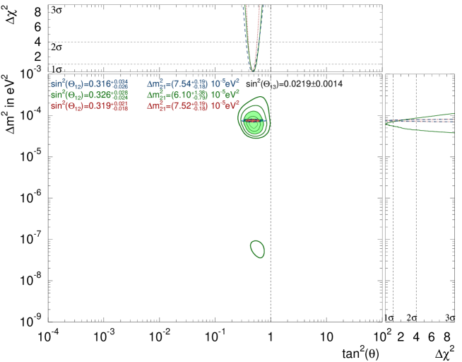
Figure 18: Oscillation parameters obtained from SK dataSOLSK2020 compared with the KamLAND reactor dataKAMLAND . The green contours show the allowed region of $\theta_{12}$ and $\Delta m^{2}_{21}$ obtained from the SK data with the ${}^{8}{\rm B}$ flux constrained by the SNO NC value((5.25$\pm 0.20)\times 10^{6}$/cm²/s). The lines show 1, 2, 3, 4 and 5$\sigma$ significance from inside to outside. The light-blue filled area shows the KamLAND reactor contour with 3$\sigma$ and the brown filled area shows the SK and KamLAND combined result with 3$\sigma$.

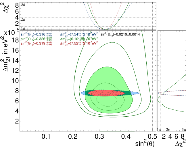
Figure 19: As for Fig.18 but the vertical axis has a linear scale. The green, light-blue and brown regions show contours of SK, KamLAND and the combination of SK and KamLAND, respectively.

Figure 20 shows the allowed region obtained by combining the SK and SNOSOLSNOCOMB data.

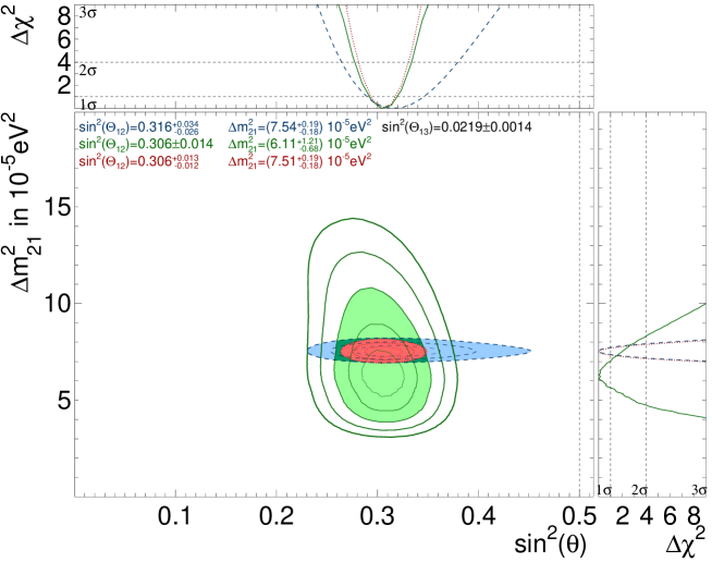
Figure 20: Oscillation parameters obtained from SK and SNO data compared with the KamLAND reactor dataKAMLAND . The green contours show the allowed region of $\theta_{12}$ and $\Delta m^{2}_{21}$ obtained from the SK and SNO data. The lines show the 1, 2, 3, 4 and 5$\sigma$ significance from inside to outside. The light-blue filled area shows the KamLAND reactor contour with 3$\sigma$, and the brown filled area shows the SK, SNO and KamLAND combined contour with 3$\sigma$.

10 Conclusion and future prospects

The solar neutrino problem suggested by the Homestake experiment lead to some very interesting outcomes. Owing to the insight of Prof. Koshiba, the solar neutrino problem was confirmed by a water Cherenkov detector, Kamiokande. The water Cherenkov technique was adopted in Super-Kamikande and SNO and precise measurements of the ${}^{8}{\rm B}$ solar neutrino flux were conducted. Especially, the flux difference between the neutral current and charged current methods, which are sensitive to all types of neutrinos and only to ${\nu}_{\rm e}$, respectively, provided smoking gun evidence of neutrino oscillations. All the results from solar neutrino experiments (Homestake, Kamiokande, SAGE, GALLEX/GNO, Super-Kamiokande, SNO and Borexino) can be shown to be consistent with the expectations from the standard solar model with neutrino oscillations. That is a great accomplishment and it could not have been done without the insight of Prof. Koshiba.

Is this the end of the story for solar neutrinos? I do not think so. The measurements of the ${}^{8}{\rm B}$ spectrum shape and the day/night difference are not yet precise enough to allow a proper discussion of neutrino oscillations. Borexino succeeded in observing CNO neutrinos but without sufficient precision to discuss the low and high metallicity models. The most abundant solar neutrino source is $pp$ neutrinos and the SSM predicts its flux with an accuracy of $\sim$1%. However, the experimental results are not yet this precise. Something interesting might still be hidden in solar neutrinos.

References

- (1) J.N. Bahcall, M.H. Pinsonneault and S. Basu, Astrophys. J. 555, 990 (2001).
- (2) J.N. Bahcall and M.H. Pinsonneault, Phys. Rev. Lett. 92, 121301 (2004).
- (3) N. Vinyoles, A. M. Serenelli, F.L. Villante, S. Basu, J. Bergström, M.C. Gonzalez-Garcia, M. Maltoni, Carlos Peña-Garay, and N. Song, Astrophys. J. 835, 202(2017).
- (4) N. Grevesse and A.J. Sauval, Space Sci. Rev. 85, 161 (1998).
- (5) M. Asplund, N. Grevesse, A.J. Sauval, and P. Scott, Annual Rev. Astron. Astrophys. 47, 481 (2009).
- (6) B. Pontecorvo, Chalk River Report PD-205 (1946).
- (7) B.T. Cleveland et al., Astrophys. J. 496, 505 (1998).
- (8) H. Georgi and S. L. Glashow, Phys. Rev. Lett. 32, 438 (1974).
- (9) K.S. Hirata et al. (Kamiokande-II Collaboration), Phys. Rev. Lett. 63, 16 (1989).
- (10) Y. Fukuda et al.(Kamiokande Collaboration), Phys. Rev. Lett. 77, 1683 (1996).
- (11) Dzh.N. Abdurashitov et al. , Phys. Lett. B328, 234 (1994).
- (12) V.N. Gavrin et al. (SAGE Collaboration), Nucl. Phys. B(Proc. Suppl.) 91, 36 (2001).
- (13) J.N. Abdurashitov et al., Phys. Rev. C80, 015807 (2009).
- (14) P. Anselmann et al. (GALLEX Collaboration), Phys.Lett. B327, 377 (1994).
- (15) P. Anselmann et al. (GALLEX Collaboration), Phys.Lett. B357, 237 (1995).
- (16) W. Hampel et al. (GALLEX Collaboration), Phys.Lett. B388, 384 (1996).
- (17) M. Altmann et al. (GNO Collaboration), Phys.Lett. B616, 174 (2005).
- (18) L. Wolfenstein, Phys. Rev. D17, 2369 (1978).
- (19) P. Langacker, J. P. Leveille and J. Sheiman, Phys. Rev. D27, 1228 (1983).
- (20) S. P. Mikheyev and A. Y. Smirnov, Sov. Jour. Nucl. Phys. 42, 913 (1985).
- (21) P. I. Krastev and S. T. Petcov, Phys. Lett. B299, 99 (1993).
- (22) N. Hata and P. Langacker, Phys.Rev. D50, 632 (1994), hep-ph/9311214.
- (23) M. Nakahata et al.(Super-Kamiokande Collaboration), Nucl. Instrum. Meth. A421, 113 (1999).
- (24) E. Blaufuss et al. (Super-Kamiokande Collaboration), Nucl. Instrum. Meth. A458, 638 (2001).
- (25) S. Fukuda et al. (Super-Kamiokande Collaboration), Phys. Rev. Lett. 86, 5651 (2001).
- (26) S. Fukuda et al. (Super-Kamiokande Collaboration), Phys. Lett. B539, 179 (2002).
- (27) J.P. Cravens et al. (Super-Kamiokande Collaboration), Phys. Rev. D78, 032002 (2008).
- (28) K. Abe et al. (Super-Kamiokande Collaboration), Phys. Rev. D83, 052010 (2011).
- (29) J. Hosaka et al. (Super-Kamiokande Collaboration), Phys. Rev. D73, 112001 (2006).
- (30) Y. Nakajima et al. (Super-Kamiokande Collaboration), Presentation at The XXIX International Conference on Neutrino Physics and Astrophysics (Neutrino 2020).
- (31) WDC-SILSO, Royal Observatory of Belgium, Brussels. http://www.sidc.be/silso/datafiles .
- (32) S. Abe et al. (KamLAND Collaboration), Phys. Rev. Lett. 100, 221803 (2008).
- (33) Q.R. Ahmad et al. (SNO Collaboration), Phys. Rev. Lett. 89, 011301 (2002).
- (34) B. Aharmim et al. (SNO Collaboration), Phys. Rev. C72, 055502 (2005).
- (35) B. Aharmim et al. (SNO Collaboration), Phys. Rev. Lett101, 111301 (2008).
- (36) B. Aharmim et al. (SNO Collaboration), Phys. Rev. C88, 025501 (2013).
- (37) C. Arpesella et al. (Borexino Collaboration), Phys. Rev. Lett. 101, 091302 (2008).
- (38) G. Bellini et al. (Borexino Collaboration), Phys. Rev. Lett. 108, 051302 (2012).
- (39) G. Bellini et al. (Borexino Collaboration), Nature 512, 383 (2014).
- (40) M. Agostini et al. (Borexino Collaboration), Nature 587, 577 (2020).
- (41) M. Agostini et al. (Borexino Collaboration), Phys. Rev. D100, 082004 (2019).
- (42) Q.R. Ahmad et al. (SNO Collaboration), Phys. Rev. Lett. 87, 071301 (2001).
- (43) F. P. An et al. (Daya Bay Collaboration), Chin. Phys. C37, 011001 (2013); J. K. Ahn et al., Phys. Rev. Lett. 108, 191802 (2012); Y. Abe et al., Phys. Rev. D86, 052008 (2012).