KinoJGM: A framework for efficient and accurate quadrotor trajectory generation and tracking in dynamic environments

Abstract

Unmapped areas and aerodynamic disturbances render autonomous navigation with quadrotors extremely challenging. To fly safely and efficiently, trajectory planners and trackers must be able to navigate unknown environments with unpredictable aerodynamic effects in real-time. When encountering aerodynamic effects such as strong winds, most current approaches to quadrotor trajectory planning and tracking will not attempt to deviate from a determined plan, even if it is risky, in the hope that any aerodynamic disturbances can be resisted by a robust controller. This paper presents a novel systematic trajectory planning and tracking framework for autonomous quadrotors. We propose a Kinodynamic Jump Space Search (Kino-JSS) to generate a safe and efficient route in unknown environments with aerodynamic disturbances. A real-time Gaussian Process is employed to model the errors caused by aerodynamic disturbances, which we then integrate with a Model Predictive Controller to achieve efficient and accurate trajectory optimization and tracking. We demonstrate our system to improve the efficiency of trajectory generation in unknown environments by up to 75% in the cases tested, compared with recent state-of-the-art. We also show that our system improves the accuracy of tracking in selected environments with unpredictable aerodynamic effects. Our implementation is available in an open source package.

I INTRODUCTION

It is crucial that autonomous Unmanned Aerial Vehicles (UAVs), such as quadrotors, can maintain their autonomy in complex and dynamic environments. Achieving safe, efficient and reliable autonomous navigation for quadrotors in GPS-denied environments, unmapped environments and/or those with large aerodynamic disturbances - e.g., strong wind or turbulence - is an ongoing challenge with considerable significance to industrial applications, such as commercial deliveries, search-and-rescue and smart agriculture.

Most existing methods on quadrotor trajectory generation and tracking have so far been demonstrated in free known space (free space here refers to unoccupied space) [1, 2, 3]. For an unknown environment and environments in which aerodynamic disturbances can jeopardize the stability of a quadrotor there are two main problems that need to be solved: How can an optimized trajectory be generated efficiently in real-time whilst guaranteeing safety and feasibility? And; How can a feasible trajectory be generated and tracked using limited onboard computational resources?

Generating optimized trajectories for quadrotors is typically solved using geometric methods for route searching [4, 5] and stitched polynomial formulation for trajectory optimization [3, 6]. However, these methods do not consider the quadrotor’s dynamic model in the route searching and optimization process, and the trajectory optimized with geometric methods that may exceed the dynamic limitations of the quadrotor. Generating and tracking feasible trajectories in dynamic environments is typically achieved by directly feeding any aerodynamic disturbances into the tracking module and controller. Such an approach does not consider the entire quadrotor system framework - e.g., route searching, trajectory optimization and tracking, and the flight controller - and leaves the quadrotor vulnerable to attempting to navigate unsuitable environments.

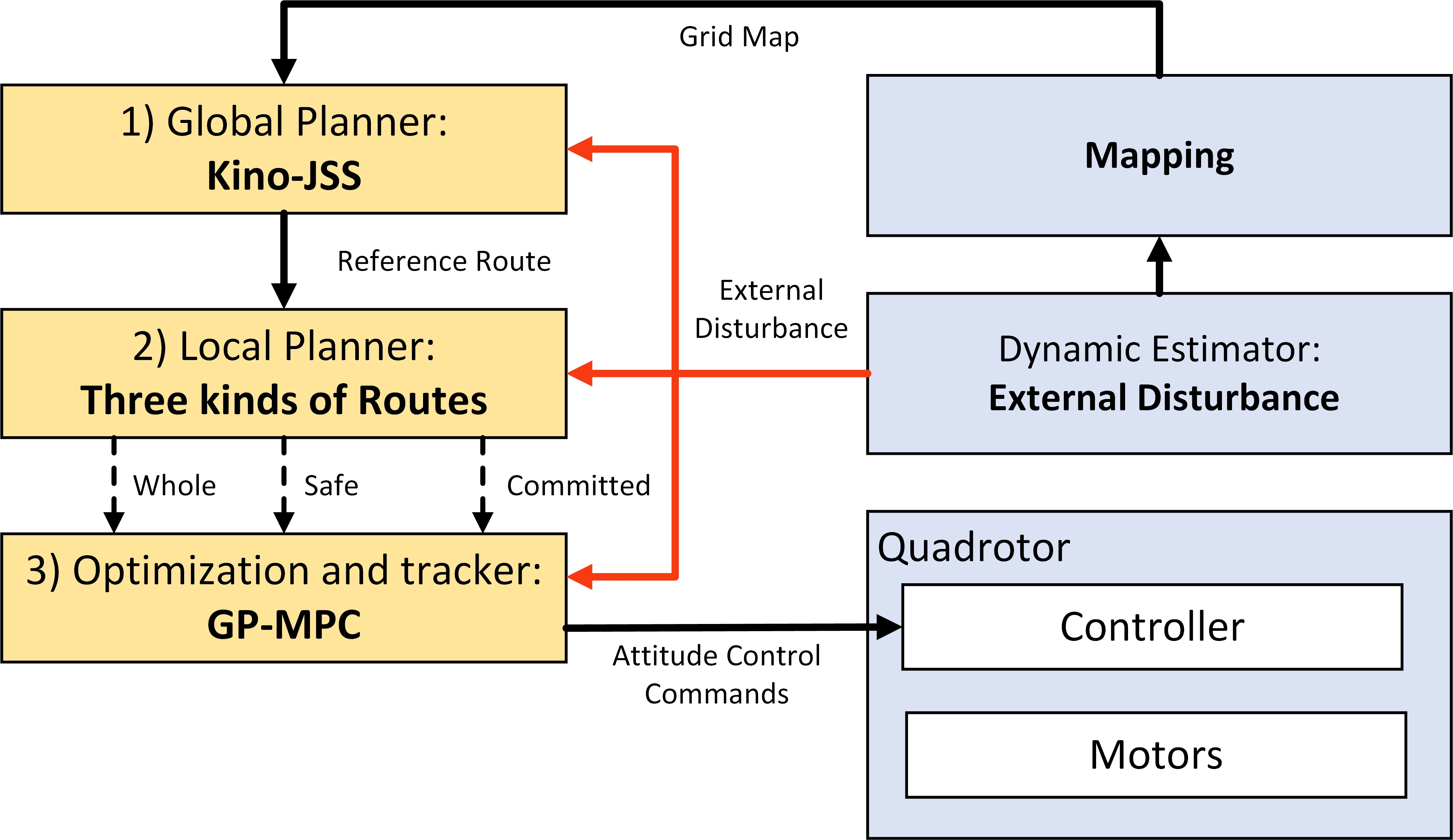
Figure 1: System overview of the KinoJGM framework: given the aerodynamic estimation, Kino-JSS (global planner), local planner and GP-MPC (optimization and tracker) generate trajectories at a high rate and give the attitude control commands to the quadrotor’s controller in real-time.

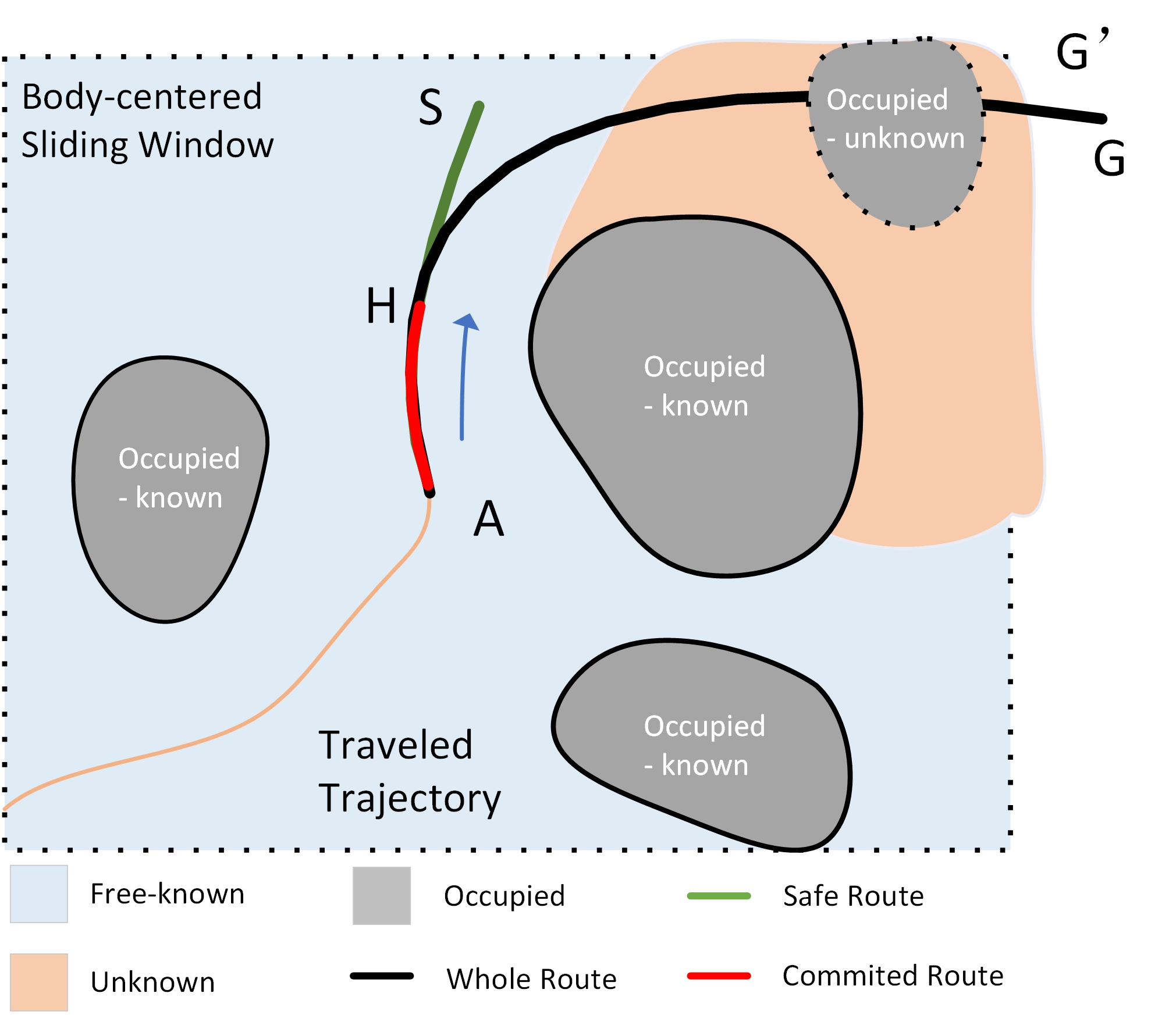
Figure 2: Local planner: whole, safe and committed routes are generated, respectively. Point A is the current position of quadrotor, G’ is the next goal position, and, G is the terminal goal position.

To address the two stated issues, we propose Kinodynamic Jump Space Search and Gaussian-Process-based Model Predictive Control (KinoJGM), a systematic, safe and feasible online trajectory generation and tracking framework for use in unknown environments with aerodynamic disturbances (shown in Fig. 1). The procedure is as follows:

1. Global Planner: a Kinodynamic Jump Space Search (Kino-JSS), described by Algorithms 1, 2 and 3, is proposed for route searching. Kino-JSS builds upon traditional Jump Point Search (JPS) [4, 5] insofar as Kino-JSS is a kinodynamic process which considers the dynamic model of the quadrotor whilst generating routes. Kino-JSS runs an order of magnitude faster than a kinodynamic search based on a hybrid-state A* search [7], whilst maintaining comparable performance. Kino-JSS can not only generate a safe and feasible original route efficiently, but can also make adjustments based on aerodynamic disturbance estimation and the quadrotor dynamic limitation.

2. Local Planner: Similar to [1], three types of route are distinguished in real-time based on the original route points given by the Kino-JSS. As shown in Figure 2, the whole route is from $A$ to $G^{\prime}$, which is efficient and has an end condition; the safe route is from $A$ to $S$; and the committed route is from $A$ to $H$, which is safe and efficient.

3. Optimization and tracker: an integrated Model Predictive Control (MPC) using Gaussian Process (GP) is proposed to optimize routes from the Local Planner and track accurately. In order to decrease the computational cost, the integrated MPC is constrained into a corresponding polyhedron [5] derived from the Local Planner routes.

Our contributions can be summarized as follows:

• Kino-JSS, a route searching algorithm with aerodynamic disturbance estimation that can efficiently generate safe and feasible routes.

• The integration of aerodynamic disturbance estimation with GP-MPC, a real-time trajectory optimization and tracking system that integrates GP into an optimal control problem constrained in polyhedrons.

• KinoJGM, a systematic trajectory planning and tracking framework verified in simulated experiments.

II Related Work

The literature on quadrotor trajectory generation and tracking is extensive and comprises a wide variety of backgrounds and perspectives - e.g., search-based methods [8, 9, 10], sampling-based methods [11, 12, 13, 14], optimization-based methods [15, 16, 17] and control-based methods [18, 19]. For brevity, we use this section to discuss the most relevant literature, which we arrange into two categories: kinodynamic trajectory planning, and robust planning with dynamic disturbance.

II-A Kinodynamic trajectory planning

Kinodynamic trajectory planning explores optimized trajectories in a high-dimensional state space and outputs a time-parameterized trajectory [20], in which quadrotor dynamics are considered. These methods - e.g., [11, 12, 13, 21] - correspond to kinematic systems which provide an efficient and easy way to achieve kinodynamic searching. An efficient kinodynamic Boundary Value Problem solver is designed by Xie et al. [22] using sequential quadratic programming. Although the efficiency of kinodynamic searching keeps improving, it remains a computationally expensive process, which limits its suitability for online planning. The work by Liu et al. [8] and Allen et al. [14] towards a real-time kinodynamic planning framework develops efficient heuristics by solving a linear quadratic minimum time problem. However, the generated trajectory is not always smooth as they use a simplified system model. Ding et al. [20, 23] propose a kinodynamic search with B-spline optimization. The uniform B-spline improves feasibility and safety for the quadrotor, but the use of non-adaptive time allocation polyhedrons can significantly reduce overall trajectory quality in some scenarios, and adding more constraints iteratively is prohibitive for real-time applications. Zhou et al. [7] propose a robust Kinodynamic-Route-Search (Kino-RS) method in discretized control space. This online kinodynamic method is robust and provides dynamic feasibility. Building on this work [7], our simulated experiments demonstrate that Kino-JSS runs an order of magnitude faster than Kino-RS [7] in obstacle-dense environments, whilst maintaining comparable system performance.

II-B Robust Planning with dynamic disturbance

Many environments require an autonomous quadrotor system to resist aerodynamic disturbances whilst planning a safe and energy-efficient path. Typically, dynamic disturbances are handled by the quadrotor’s tracking module and flight controller [24, 25], because robust control is generally designed for the “worst-case” bounded uncertainties and disturbances [26]. Adaptive controllers [27] can address some of the problems caused by aerodynamic disturbances with unknown boundaries, but the system needs to be continuously updated with vehicle state estimations for effective control. For a quadrotor, this can cause undesired high-frequency oscillation behaviours. Singh et al. [28], Guerrero [29] and Palmieri [30] design a global planner for a simulated quadrotor flying in areas with aerodynamic disturbances. However, this method is tested in highly controlled simulated environments, and assumes accurate aerodynamic disturbance estimation.

MPC is an efficient tool to generate optimal local trajectories and encode uncertainty arising from aerodynamic disturbances. In [31], GP is used on a quadrotor to correct for wind disturbances. Hewing et al. [32], Kabzan et al. [33] and Torrente et al. [34] design and implement a GP-MPC method to accurately predict small aerodynamic disturbances and improve tracking accuracy for autonomous vehicles. Building on these works [32, 33, 34], we integrate GP and MPC, but extend to large aerodynamic disturbances - e.g., strong winds and those generated by the quadrotor and environmental obstacles. Our proposed GP-MPC sets the estimation of aerodynamic disturbance as a value in formulation (Equation 2 and Equation 3) to generate optimized trajectories and perform accurate tracking in real-time.

III Methodology

In this section, we present the proposed KinoJGM framework and its novel modules. This work addresses the current limitations on route searching and trajectory planning in unknown environments with aerodynamic disturbances. The modules that comprise our KinoJGM framework are described as follows.

III-A Mapping Module

In practice, drone flight is oftentimes desirable in GPS-denied environments, where on-board sensing will be relied on for state estimations - e.g., position, velocity, acceleration and jerk. The accumulation of drift is therefore a significant problem when operating in complex and/or large environments. We use a body-centered sliding window, as described in [1], [35], and shown in Figure 2, to reduce the influence of drift in state estimation error.

III-B Aerodynamic Disturbance Estimation Module

We use Visual-Inertial-Dynamics-Fusion (VID-Fusion) [36] to estimate the aerodynamic disturbance operating on the quadrotor at a given time. VID-Fusion is a tightly coupled state estimator for quadrotors. It compares the quadrotor dynamic model with the inertial measurement unit (IMU) reading - i.e., Visual-Inertial-System-Monocular (VINS-mono) [37] and Visual Inertial Model-Based Odometry (VIMO) [38] - to generate robust and accurate aerodynamic disturbance and pose estimation.

III-C Route Searching Module (Kino-JSS)

Quadrotor route searching primarily focuses on robustness, feasibility and efficiency. The Kino-RS algorithm [7] is a robust and feasible online searching approach. However, the searching loop is derived from the hybrid-state A* algorithm, making it relatively inefficient in obstacle-dense environments. On the other hand, JPS offers robust route searching, and runs at an order of magnitude faster than the A* algorithm [4]. A common problem of geometric methods such as JPS and A* is that, unlike kinodynamic searching, they consider heuristic cost (e.g., distance) but not the quadrotor dynamics and feasibility (e.g., line 5 of Algorithm 2 and line 10 of Algorithm 3) when generating routes [20]. $\bf{checkFea()}$ is the feasibility check to judge the acceleration and velocity constrains based on the quadrotor dynamics. Kino-JSS is described by Algorithms 1, 2 and 3.

Algorithm 1 Kinodynamic Jump Space Search

INPUT: $s_{cur}$
OUTPUT: $KinoJSSRoute$

1:  $\bf{initialize()}$

2:  $openSet.\bf{insert(\it{s_{cur}})}$

3:  while !$openSet.\bf{isEmpty()}$ do

4:     $s_{cur}\leftarrow openSet.\bf{pop()}$

5:     $closeSet.\bf{insert(\it{s_{cur}})}$

6:     if $\bf{nearGoal(\it{s_{cur}})}$ then

7:        return  $KinoJSSRoute$

8:     end if

9:     $\bf{KinoJSSRecursion()}$

10:  end while

Algorithm 2 KinoJSSRecursion

INPUT: $s_{cur}$, $E_{f}$, $openSet$, $closeSet$
OUTPUT: $void$

1:  $motions\leftarrow\bf{JSSMotion(\it{s_{cur},E_{f}})}$

2:  for each $m_{i}\in motions$ do

3:     $s_{pro}\leftarrow\bf{statePropagation(\it{s_{cur},m_{i}}))}$

4:     $inClose\leftarrow\it{closeSet}.\bf{isContain(\it{s_{pro}})}$

5:     if $\bf{isFree(\it{s_{pro}})}\bigwedge\bf{checkFea(\it{s_{pro},m_{i}})}\bigwedge\it{inClose}$ then

6:        if  $\bf{checkOccupiedAround(\it{s_{pro}})}$ then

7:           $s_{pro}.neighbors\leftarrow\bf{JSSNeighbor(\it{s_{pro}})}$

8:           $cost_{pro}\leftarrow\it{s_{cur}}.cost+\bf{edgeCost(\it{s_{pro}})}$

9:           $cost_{pro}\leftarrow cost_{pro}+\bf{heuristic(\it{s_{pro}})}$

10:           if !$\it{openSet}.\bf{isContain(\it{s_{pro}})}$ then

11:              $openSet.\bf{insert(\it{s_{pro}})}$

12:           else if $\it{s_{pro}}.cost\leq\it{cost_{pro}}$ then

13:              continue

14:           end if

15:           $s_{pro}.parent\leftarrow s_{cur}$

16:           $s_{pro}.cost\leftarrow cost_{pro}$

17:        else

18:           $\bf{KinoJSSRecursion()}$

19:        end if

20:     else

21:        continue

22:     end if

23:  end for

Algorithm 3 JSSMotion

INPUT: $s_{cur}$, $E_{f}$
OUTPUT: $motions$

1:  $E_{fcor}\leftarrow E_{f}+\bf{GaussianNoise()}$

2:  for each $m_{i}\in motionSet$ do

3:     $m_{cor}\leftarrow m_{i}+E_{fcor}$

4:     $motions\leftarrow\bf{push\_back(\it{m_{cor}})}$

5:  end for

6:  $neighSize\leftarrow s_{cur}.neighbors.\bf{size()}$

7:  while $neighSize\neq 0$ do

8:     $neighSize=neighSize-1$

9:     $neighMotion\leftarrow\bf{posToMotion(\it{s_{cur}.neighbors)}}$

10:     if $\bf{checkFea(\it{s_{cur},neighMotion})}$ then

11:        $motions\leftarrow\bf{push\_back(\it{neighMotion})}$

12:     end if

13:  end while

14:  return  $motions$

$s_{cur}$ denotes the current state, $s_{pro}$ denotes the propagation of current state under the motion $m_{i}$, and $E_{f}$ denotes the aerodynamic disturbance estimated by VID-fusion [36]. In Algorithm 2, $\bf{JSSNeighbor()}$ is defined as shown in Fig. 3. In Algorithm 3, $motionSet$, which is defined as a pyramid shown in Fig. 4, offers improved efficiency whilst retaining the advantages of Kino-RS [7].

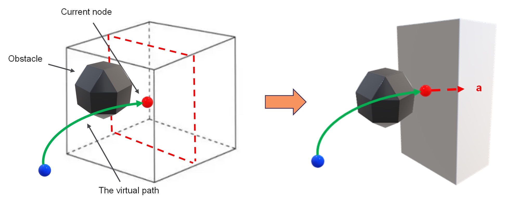
Figure 3: Diagram of KinoJSS when checking occupied obstacles around: a grey cuboid is generated as the ‘forced neighbour’, the output of $\bf{JSSNeighbor()}$, in Algorithm 2.

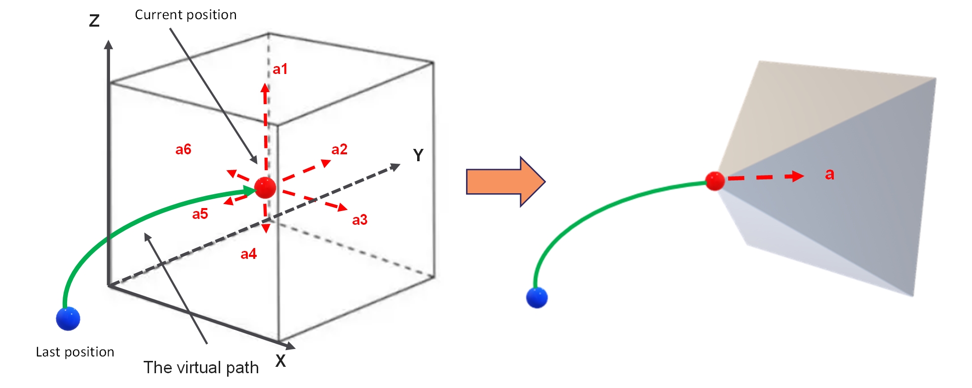
Figure 4: Diagram of KinoJSS with unoccupied space around: the pyramid represents the $motionSet$ in Algorithm 3, i.e., $\bf{JSSMotion()}$, in free space.

III-D Trajectory Optimization and Tracking Module (GP-MPC)

Traditional approaches [1, 5] address trajectory optimization and tracking separately. This partitioned solution seems to be logical and each process is easy to analyze in isolation. On the other hand, integrating the trajectory optimization and tracking processes increases the search space and computing complexity, which limits the quadrotor’s ability to react dynamically in real-time [39]. We use an integrated MPC-based approach that generates an optimized trajectory and a sequence of tracking commands by solving an optimal control problem. Trajectory optimization and tracking is achieved using GP-MPC, which combines with a full-state quadrotor MPC formulation [40, 41, 34].

We integrate the aerodynamic force (disturbance) $\bm{e}_{f}$ into the dynamic model of a quadrotor as follows:

$$\dot{\bm{P}}_{WB}=\bm{V}_{WB}$$ (1)

$$\dot{\bm{V}}_{WB}=\bm{g}_{W}+\frac{1}{m}(\bm{q}_{WB}\odot\bm{c}+\bm{e}_{f})$$

$$\dot{\bm{q}}_{WB}=\frac{1}{2}\Lambda(\bm{\omega}_{B})\bm{q}_{WB}$$

$$\dot{\bm{\omega}}_{B}=\bm{J}^{-1}(\bm{\tau}_{B}-\bm{\omega}\times J\bm{\omega}_{B})$$

where $\bm{P}_{WB}$, $\bm{V}_{WB}$ and $\bm{q}_{WB}$ are the position, linear velocity and orientation of the quadrotor expressed in the world frame (shown in Fig. 5), and $\bm{\omega}_{B}$ is the angular velocity expressed in the body frame [34]. The state of the dynamic model - i.e., $\bm{x}=[\bm{P}_{WB},\bm{V}_{WB},\bm{q}_{WB},\bm{\omega}_{B}]^{T}$ - is used for quadrotor motion planning. The input vector of the dynamic model is $\bm{u}=T_{i}\forall i\in(0,3)$. $\bm{c}$ is the collective thrust $\bm{c}=[0,0,\sum T_{i}]^{T}$ and $\bm{\tau}_{B}$ is the body torque; $\bm{g}_{W}=[0,0,-g]^{T}$. The operator $\odot$ denotes a rotation of the vector by the quaternion. We assume that the aerodynamic force $\bm{e}_{f}$ in Equation 1 only effects the position motion of quadrotor and not its angular motion. The skewsymmetric matrix $\Lambda(\bm{\omega})$ is defined in [41].

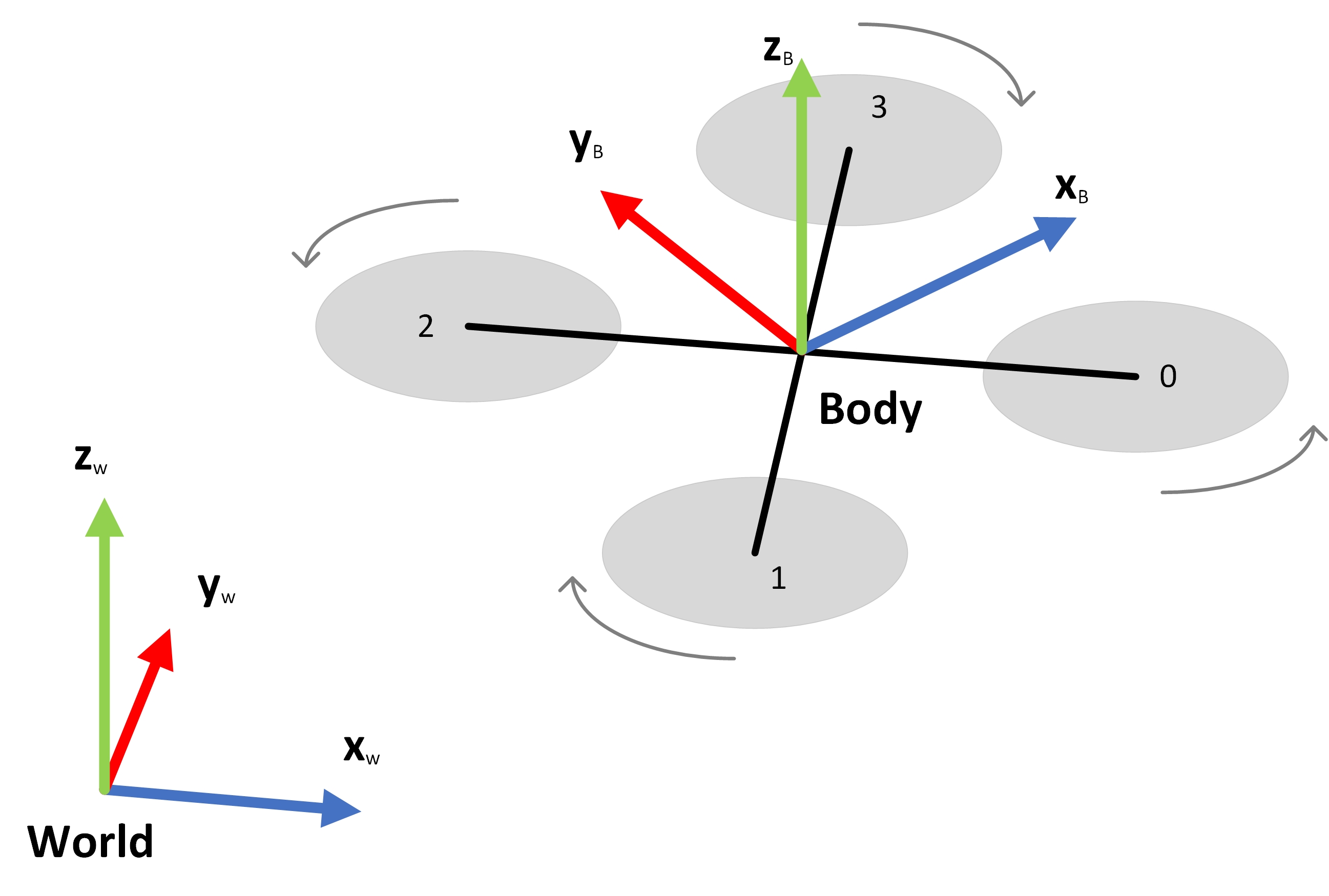
Figure 5: Diagram of the quadrotor the world frame W and the body frame B.

For integration in a discrete-time MPC, the quadrotor dynamic model is discretized using a Runge-Kutta 4th-order integration [32] with sampling time $T_{s}=50ms$. As per [36], the nominal force $\bm{n_{f}}$ can be treated as a constant value calculated in short duration, and the aerodynamic force estimation is defined as: $\bm{e}_{fk}=\bm{n_{f}}+\bm{w}_{k}$, where $\bm{w}_{k}\sim\mathcal{N}(0,\sigma)$ is Gaussian noise. So, the discrete-time state $\bm{x}_{k}$ is defined as:

$$\bm{x}_{k+1}=\bm{f}_{RK}(\bm{x}_{k},\bm{u}_{k},\bm{e_{fk}})$$ (2)

We define the control of the quadrotor dynamic model with a discrete-time model:

$$\bm{x}_{k+1}=\bm{f}(\bm{x}_{k},\bm{u}_{k},\bm{e_{fk}})+\bm{B}_{d}(\bm{g}(\bm{x}_{k},\bm{u}_{k})+\bm{w}_{k})$$ (3)

where $B_{d}$ is the selection matrix, $\bm{g}$ describes an initially unknown dynamic model, and, both $\bm{f}$ and $\bm{g}$ are assumed to be differentiable functions.

In GP-MPC, GP is used to predict the error of the dynamic model. Like most GP-based approaches, e.g., [32, 33, 34], we formulate this by assuming a true value $\bm{f}_{true}$ and a measurement value $\tilde{\bm{x}}_{k+1}=\bm{f}_{mea}$:

$$\tilde{\bm{x}}_{k+1} =\bm{f}_{mea}(\bm{x}_{k},\bm{u}_{k},\bm{e_{fk}})$$ (4)

$$=\bm{f}_{true}(\bm{x}_{k},\bm{u}_{k},\bm{e_{fk}})+\bm{w}_{k}$$

where $\bm{w}_{k}\sim\mathcal{N}(0,\sigma)$ is the process noise and $\sum$ is a diagonal variance matrix.

We use the rational quadratic kernel as a kernel function $\bm{k}(\bm{z}_{i},\bm{z}_{j})$ which is defined by:

$$\bm{k}(\bm{z}_{i},\bm{z}_{j})=\sigma_{f}^{2}(1+\frac{(\bm{z}_{i}-\bm{z}_{j})^{T}L^{-2}(\bm{z}_{i}-\bm{z}_{j})}{2\alpha})^{-\alpha}+\sigma_{n}^{2}$$ (5)

where $L$ is the diagonal length scale matrix; $\sigma_{f}$ and $\sigma_{n}$ represent the data and prior noise variance; and, $\bm{z}_{i}$,$\bm{z}_{j}$ represents data features. Then, the mean and covariance of the GP is defined as follows:

$$\bm{\mu}(Z)= (\bm{k}(Z,Z_{k}))^{T}(\bm{k}(Z,Z)+\sigma_{n}^{2}I)^{-1}Z$$ (6)

$$\Sigma(Z)= \bm{k}(Z_{k},Z_{k})$$

$$-(\bm{k}(Z,Z_{k}))^{T}(\bm{k}(Z,Z)+\sigma_{n}^{2}I)^{-1}\bm{k}(Z,Z_{k})$$

where $Z$ and $Z_{k}$ denote the training input and test samples. Given the mean and covariance of the GP, we calculate the modified dynamic and feed it into the MPC formulation as follows:

$$\mathop{min}\limits_{u}L(\bm{x},\bm{u})= \bm{x}_{N}^{T}Q\bm{x}_{N}+\sum_{k=0}^{N}\bm{x}_{k}^{T}Q\bm{x}_{k}+\bm{u}_{N}^{T}R\bm{u}_{N}$$ (7)

$$\rm{subject}\quad\rm{to} \bm{x}_{k+1}=\bm{f}(\bm{x_{k}},\bm{u_{k}},\bm{e_{fk}})$$

$$\bm{x_{0}}=\bm{g}(\bm{x_{k}},\bm{u_{k}})$$

$$\bm{u_{min}}\leq\bm{u}\leq\bm{u_{max}}$$

The quadratic optimization formulation in Equation 7 is discretized based on the multiple shooting method [42] and solved using sequential quadratic programming for real-time motion planning [42]. We implement the calculation of the MPC formulation using CasADi [43] and ACADOS [44].

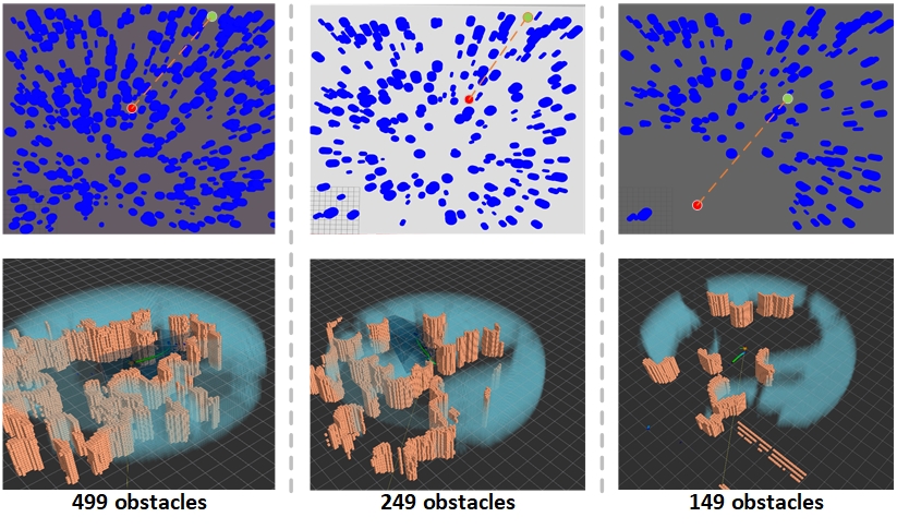
Figure 6: Three kinds of environment with different obstacles (499, 249 and 149 obstacles) in the simulation.

IV Implementation and Results

IV-A Setup

We evaluate the performance of our proposed trajectory generation and tracking framework in software simulation, in which a DJI Manifold 2-C (Intel i7-8550U CPU) is used for real-time computation. We use RotorS MAVs simulator [45], in which programmable aerodynamic disturbances can be generated, for testing the KinoJGM framework. As shown in Section III-D, the aerodynamic disturbance is defined and simulated as a nominal force $\bm{n_{f}}$ plus Gaussian noise $\bm{w}_{k}$. The nominal force $\bm{n_{f}}$ is estimated by VID-Fusion [36]. The noise bound of aerodynamic disturbance is set as 0.5 $m/s^{2}$, based on the benchmark established in [46]. We first test the Kino-JSS (route searching) module against the system described in [7], before comparing our entire KinoJGM framework with the system described in [46]. Since the update frequency of the aerodynamic force $\bm{e_{f}}$ estimation is much higher than our KinoJGM framework frequency, we sample $\bm{e_{f}}$ based on our framework frequency. We also assume the collective thrust $\bm{c}$ is a true value, which is tracked ideally in the simulation platform.

IV-B Experiments

TABLE I: Comparison of Route Searching

		499 Obstacles			249 Obstacles			149 Obstacles
		Time (ms)	Ctrl cost	Succ. Rate	Time (ms)	Ctrl cost	Succ. Rate	Time (ms)	Ctrl cost	Succ. Rate
Zhou. [7]	Mean	70.3664	57.73	78.60%	39.6634	46.11	100.00%	23.6290	21.25	100.00%
	Std	55.5857	29.78		32.7760	28.94		13.7430	36.78
	Max	236	101.18		232	97.25		75	98.31
Kino-JSS	Mean	17.3782	48.12	79.61%	13.1701	28.75	100.00%	10.9858	19.59	100.00%
	Std	10.8848	11.30		7.5069	15.56		5.8236	27.36
	Max	106	72.06		39	61.02		34	58.38

1) Comparative performance of Kino-JSS route searching module: We compare our Kino-JSS module with Zhou et al. [7], which uses a Kino-RS method to generate route points. The comparison is on a $40m\times 40m\times 5m$ map, where 1m of simulated space corresponds to 0.15m of real space. The maximum quadrotor velocity and acceleration are set as $3m/s$ and $2m/s^{2}$, respectively (in real space). These parameters are equivalent to those used by Zhou et al. [7]. As shown in Figure 6, we perform experiments in simulated environments with 499, 249 and 149 obstacles to demonstrate our system’s performance in environments of varying obstacle-density.

Unlike Kino-RS [7], Kino-JSS will not add a search point to the $openSet$ until an obstacle is encountered. This characteristic of Kino-JSS means that more space can be searched per operation, and substantially increases the efficiency of Kino-JSS over Kino-RS in obstacle-dense environments. This is demonstrated by our results given in Table I. The improved efficiency of Kino-JSS is most evident in areas with highest obstacle density, where we achieve improvements of 75%, 67% and 53% for environments with 499, 249 and 149 obstacles, respectively. Predictably, the improvement in efficiency for Kino-JSS decreases with lower obstacle density, since it is proved in [4] that the performance of a JPS algorithm is equivalent with an A* algorithm in free environments. Our results also show that the quadrotor control cost of Kino-JSS is much lower than Kino-RS, because Kino-JSS can jump way-points and only operates way-points with forced neighbours, also shown in line 7 of Algorithm 2 and line 1 of Algorithm 3.

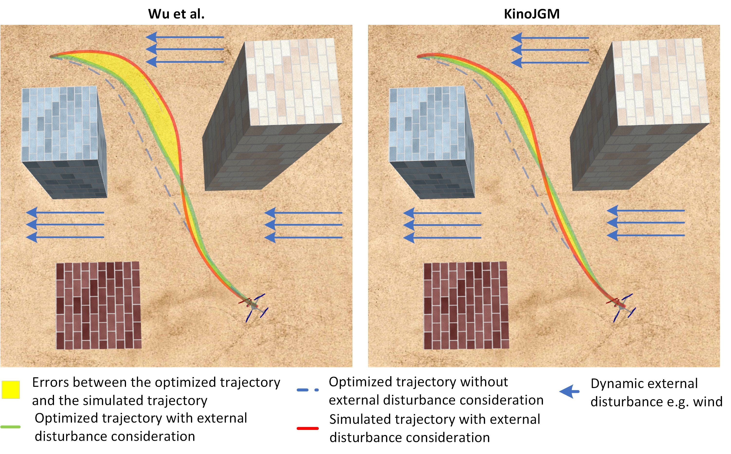
Figure 7: The comparison between Wu et al. [46] and our proposed KinoJGM framework.

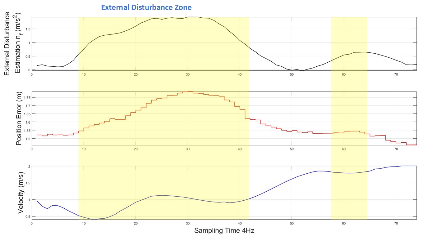
Figure 8: The simulation results: aerodynamic disturbance estimation $n_{f}(m/s^{2})$, position error $(m)$ and velocity $(m/s)$.

2) Comparative performance of KinoJGM trajectory optimization and tracking framework: This simulation is based on the dynamic model described in Equation 1 and uses a Runge-Kutta integration to solve Equation 7 with $T_{s}=50ms$ and time steps $N=20$ [46]. The implementation of GP-MPC mainly has two phases: training and prediction. In training, the data set for the GP model is collected by following aggressive trajectories [34] with the quadrotor. After the training set collection, we use the learning results to fit the GP-MPC. The training data set is collected with the velocity range $[-3,3]m/s$.

We compare our method against a state-of-the-art trajectory optimization and tracking algorithm, ‘Wu. [46]’, with dynamic aerodynamic disturbances added to our simulated environment. Wu. [46] uses a Kino-RS proposed by ‘Zhou. [7]’ to achieve route points and a Nolinear MPC (NMPC) to generate optimized trajectory and precise tracking. In Table II, the second method, ‘Zhou. + GP-MPC’, is a combination with Kino-RS algorithm (proposed in Zhou. [7]) and GP-MPC. The results show that the GP-MPC tracking has better accuracy than NMPC in tracking. Without consideration for the aerodynamic disturbance, the second method has the lowest success rate and largest latency of the test scenarios. We can also see our KinoJGM has a greater success rate, efficiency and accuracy when handling large and complex aerodynamic disturbances. Figure 7 shows that our proposed KinoJGM framework has smaller position errors (yellow areas) than Wu et al. [46]. The aerodynamic disturbance estimation $n_{f}$, position error and quadrotor velocity in our simulated environment are shown in Figure 8.

TABLE II: Comparison of Trajectory Optimization and Tracking

Ex. disturbance	Method	Succ. Rate	Time (s)	Err. (m)
[0.0, 2.0, 0.0]	Wu. [46]	90%	9.98	5.17
	Zhou. + GP-MPC	80%	13.61	4.1
	KinoJGM	90%	7.32	1.60
[-1.0, 2.0, 0.0]	Wu. [46]	75%	14.3	6.11
	Zhou. + GP-MPC	70%	13.8	5.33
	KinoJGM	80%	9.76	2.19

V CONCLUSIONS

In this paper, we propose a complete online trajectory planning and tracking framework for unknown environments with dynamic disturbances. The framework integrates route search, trajectory optimization and tracking algorithms to overcome the effects of aerodynamic disturbances. We adopt a kinodynamic route searching method to improve our framework’s efficiency whilst maintaining optimality. Using GP to augment the noise on our dynamic model of the quadrotor, an MPC significantly improves the accuracy of position tracking. We incorporate aerodynamic disturbance into the entire framework, both in planning and tracking. We demonstrate that our proposed approach can generate a trajectory efficiently and track it precisely, and that our approach compares favourably with selected benchmarks, i.e., [7] and [46], in simulation. Our ongoing work concerns demonstrating KinoJGM in real-world tests. We will also investigate adaptive methods for aerodynamic disturbance control, such as Bayesian Optimization MPC and Reinforcement Learning.

References

- [1] Jesus Tordesillas and Jonathan P How. FASTER: Fast and safe trajectory planner for navigation in unknown environments. IEEE Transactions on Robotics, 2021.
- [2] Markus Ryll, John Ware, John Carter, and Nick Roy. Efficient trajectory planning for high speed flight in unknown environments. In 2019 International Conference on Robotics and Automation (ICRA), pages 732–738. IEEE, 2019.
- [3] Daniel Mellinger and Vijay Kumar. Minimum snap trajectory generation and control for quadrotors. In 2011 IEEE international conference on robotics and automation, pages 2520–2525. IEEE, 2011.
- [4] Daniel Harabor and Alban Grastien. Online graph pruning for pathfinding on grid maps. In Proceedings of the AAAI Conference on Artificial Intelligence, volume 25, 2011.
- [5] Sikang Liu, Michael Watterson, Kartik Mohta, Ke Sun, Subhrajit Bhattacharya, Camillo J Taylor, and Vijay Kumar. Planning dynamically feasible trajectories for quadrotors using safe flight corridors in 3-d complex environments. IEEE Robotics and Automation Letters, 2(3):1688–1695, 2017.
- [6] Charles Richter, Adam Bry, and Nicholas Roy. Polynomial trajectory planning for aggressive quadrotor flight in dense indoor environments. In Robotics research, pages 649–666. Springer, 2016.
- [7] Boyu Zhou, Fei Gao, Luqi Wang, Chuhao Liu, and Shaojie Shen. Robust and efficient quadrotor trajectory generation for fast autonomous flight. IEEE Robotics and Automation Letters, 4(4):3529–3536, 2019.
- [8] Sikang Liu, Nikolay Atanasov, Kartik Mohta, and Vijay Kumar. Search-based motion planning for quadrotors using linear quadratic minimum time control. In 2017 IEEE/RSJ international conference on intelligent robots and systems (IROS), pages 2872–2879. IEEE, 2017.
- [9] Sikang Liu, Kartik Mohta, Nikolay Atanasov, and Vijay Kumar. Search-based motion planning for aggressive flight in se (3). IEEE Robotics and Automation Letters, 3(3):2439–2446, 2018.
- [10] Sandip Aine, Siddharth Swaminathan, Venkatraman Narayanan, Victor Hwang, and Maxim Likhachev. Multi-heuristic a. The International Journal of Robotics Research, 35(1-3):224–243, 2016.
- [11] Dustin J Webb and Jur Van Den Berg. Kinodynamic rrt*: Asymptotically optimal motion planning for robots with linear dynamics. In 2013 IEEE international conference on robotics and automation, pages 5054–5061. IEEE, 2013.
- [12] Lucas Janson, Edward Schmerling, Ashley Clark, and Marco Pavone. Fast marching tree: A fast marching sampling-based method for optimal motion planning in many dimensions. The International journal of robotics research, 34(7):883–921, 2015.
- [13] Jonathan D Gammell, Siddhartha S Srinivasa, and Timothy D Barfoot. Batch informed trees (bit*): Sampling-based optimal planning via the heuristically guided search of implicit random geometric graphs. In 2015 IEEE international conference on robotics and automation (ICRA), pages 3067–3074. IEEE, 2015.
- [14] Ross Allen and Marco Pavone. A real-time framework for kinodynamic planning with application to quadrotor obstacle avoidance. In AIAA Guidance, Navigation, and Control Conference, page 1374, 2016.
- [15] Fei Gao and Shaojie Shen. Online quadrotor trajectory generation and autonomous navigation on point clouds. In 2016 IEEE International Symposium on Safety, Security, and Rescue Robotics (SSRR), pages 139–146. IEEE, 2016.
- [16] Jing Chen, Tianbo Liu, and Shaojie Shen. Online generation of collision-free trajectories for quadrotor flight in unknown cluttered environments. In 2016 IEEE International Conference on Robotics and Automation (ICRA), pages 1476–1483. IEEE, 2016.
- [17] Helen Oleynikova, Michael Burri, Zachary Taylor, Juan Nieto, Roland Siegwart, and Enric Galceran. Continuous-time trajectory optimization for online uav replanning. In 2016 IEEE/RSJ international conference on intelligent robots and systems (IROS), pages 5332–5339. IEEE, 2016.
- [18] Jur Van Den Berg, David Wilkie, Stephen J Guy, Marc Niethammer, and Dinesh Manocha. Lqg-obstacles: Feedback control with collision avoidance for mobile robots with motion and sensing uncertainty. In 2012 IEEE International Conference on Robotics and Automation, pages 346–353. IEEE, 2012.
- [19] Daman Bareiss, Jur van den Berg, and Kam K Leang. Stochastic automatic collision avoidance for tele-operated unmanned aerial vehicles. In 2015 IEEE/RSJ International Conference on Intelligent Robots and Systems (IROS), pages 4818–4825. IEEE, 2015.
- [20] Wenchao Ding, Wenliang Gao, Kaixuan Wang, and Shaojie Shen. An efficient b-spline-based kinodynamic replanning framework for quadrotors. IEEE Transactions on Robotics, 35(6):1287–1306, 2019.
- [21] Steven M LaValle and James J Kuffner Jr. Randomized kinodynamic planning. The international journal of robotics research, 20(5):378–400, 2001.
- [22] Christopher Xie, Jur van den Berg, Sachin Patil, and Pieter Abbeel. Toward asymptotically optimal motion planning for kinodynamic systems using a two-point boundary value problem solver. In 2015 IEEE International Conference on Robotics and Automation (ICRA), pages 4187–4194. IEEE, 2015.
- [23] Wenchao Ding, Wenliang Gao, Kaixuan Wang, and Shaojie Shen. Trajectory replanning for quadrotors using kinodynamic search and elastic optimization. In 2018 IEEE International Conference on Robotics and Automation (ICRA), pages 7595–7602. IEEE, 2018.
- [24] Ruiting Yu, Qidan Zhu, Guihua Xia, and Zhe Liu. Sliding mode tracking control of an underactuated surface vessel. IET control theory & applications, 6(3):461–466, 2012.
- [25] Xiangbin Liu, Hongye Su, Bin Yao, and Jian Chu. Adaptive robust control of a class of uncertain nonlinear systems with unknown sinusoidal disturbances. In 2008 47th IEEE Conference on Decision and Control, pages 2594–2599. IEEE, 2008.
- [26] Qingrui Zhang, Wei Pan, and Vasso Reppa. Model-reference reinforcement learning control of autonomous surface vehicles. In 2020 59th IEEE Conference on Decision and Control (CDC), pages 5291–5296. IEEE, 2020.
- [27] Karl J Åström and Björn Wittenmark. Adaptive control. Courier Corporation, 2013.
- [28] Sumeet Singh, Anirudha Majumdar, Jean-Jacques Slotine, and Marco Pavone. Robust online motion planning via contraction theory and convex optimization. In 2017 IEEE International Conference on Robotics and Automation (ICRA), pages 5883–5890. IEEE, 2017.
- [29] Jose Alfredo Guerrero, Juan-Antonio Escareño, and Yasmina Bestaoui. Quad-rotor mav trajectory planning in wind fields. In 2013 IEEE International Conference on Robotics and Automation, pages 778–783. IEEE, 2013.
- [30] Luigi Palmieri, Tomasz P Kucner, Martin Magnusson, Achim J Lilienthal, and Kai O Arras. Kinodynamic motion planning on gaussian mixture fields. In 2017 IEEE International Conference on Robotics and Automation (ICRA), pages 6176–6181. IEEE, 2017.
- [31] Mohit Mehndiratta and Erdal Kayacan. Gaussian process-based learning control of aerial robots for precise visualization of geological outcrops. In 2020 European Control Conference (ECC), pages 10–16. IEEE, 2020.
- [32] Lukas Hewing, Juraj Kabzan, and Melanie N Zeilinger. Cautious model predictive control using gaussian process regression. IEEE Transactions on Control Systems Technology, 28(6):2736–2743, 2019.
- [33] Juraj Kabzan, Lukas Hewing, Alexander Liniger, and Melanie N Zeilinger. Learning-based model predictive control for autonomous racing. IEEE Robotics and Automation Letters, 4(4):3363–3370, 2019.
- [34] Guillem Torrente, Elia Kaufmann, Philipp Föhn, and Davide Scaramuzza. Data-driven mpc for quadrotors. IEEE Robotics and Automation Letters, 6(2):3769–3776, 2021.
- [35] Lukas Schmid, Victor Reijgwart, Lionel Ott, Juan Nieto, Roland Siegwart, and Cesar Cadena. A unified approach for autonomous volumetric exploration of large scale environments under severe odometry drift. IEEE Robotics and Automation Letters, 6(3):4504–4511, 2021.
- [36] Ziming Ding, Tiankai Yang, Kunyi Zhang, Chao Xu, and Fei Gao. Vid-fusion: Robust visual-inertial-dynamics odometry for accurate external force estimation. arXiv preprint arXiv:2011.03993, 2020.
- [37] Tong Qin, Peiliang Li, and Shaojie Shen. Vins-mono: A robust and versatile monocular visual-inertial state estimator. IEEE Transactions on Robotics, 34(4):1004–1020, 2018.
- [38] Barza Nisar, Philipp Foehn, Davide Falanga, and Davide Scaramuzza. Vimo: Simultaneous visual inertial model-based odometry and force estimation. IEEE Robotics and Automation Letters, 4(3):2785–2792, 2019.
- [39] Michael Neunert, Cédric De Crousaz, Fadri Furrer, Mina Kamel, Farbod Farshidian, Roland Siegwart, and Jonas Buchli. Fast nonlinear model predictive control for unified trajectory optimization and tracking. In 2016 IEEE international conference on robotics and automation (ICRA), pages 1398–1404. IEEE, 2016.
- [40] Mark W Mueller, Markus Hehn, and Raffaello D’Andrea. A computationally efficient motion primitive for quadrocopter trajectory generation. IEEE transactions on robotics, 31(6):1294–1310, 2015.
- [41] Davide Falanga, Philipp Foehn, Peng Lu, and Davide Scaramuzza. Pampc: Perception-aware model predictive control for quadrotors. In 2018 IEEE/RSJ International Conference on Intelligent Robots and Systems (IROS), pages 1–8. IEEE, 2018.
- [42] Moritz Diehl, Hans Georg Bock, Holger Diedam, and P-B Wieber. Fast direct multiple shooting algorithms for optimal robot control. In Fast motions in biomechanics and robotics, pages 65–93. Springer, 2006.
- [43] Joel AE Andersson, Joris Gillis, Greg Horn, James B Rawlings, and Moritz Diehl. Casadi: a software framework for nonlinear optimization and optimal control. Mathematical Programming Computation, 11(1):1–36, 2019.
- [44] Robin Verschueren, Gianluca Frison, Dimitris Kouzoupis, Niels van Duijkeren, Andrea Zanelli, Rien Quirynen, and Moritz Diehl. Towards a modular software package for embedded optimization. IFAC-PapersOnLine, 51(20):374–380, 2018.
- [45] Fadri Furrer, Michael Burri, Markus Achtelik, and Roland Siegwart. Rotors—a modular gazebo mav simulator framework. In Robot operating system (ROS), pages 595–625. Springer, 2016.
- [46] Yuwei Wu, Ziming Ding, Chao Xu, and Fei Gao. External forces resilient safe motion planning for quadrotor. arXiv preprint arXiv:2103.11178, 2021.