Flat Latent Manifolds for Human-machine Co-creation of Music

Abstract

The use of machine learning in artistic music generation leads to controversial discussions of the quality of art, for which objective quantification is nonsensical. We therefore consider a music-generating algorithm as a counterpart to a human musician, in a setting where reciprocal interplay is to lead to new experiences, both for the musician and the audience. To obtain this behaviour, we resort to the framework of recurrent Variational Auto-Encoders (VAE) and learn to generate music, seeded by a human musician. In the learned model, we generate novel musical sequences by interpolation in latent space. Standard VAEs however do not guarantee any form of smoothness in their latent representation. This translates into abrupt changes in the generated music sequences. To overcome these limitations, we regularise the decoder and endow the latent space with a flat Riemannian manifold, i.e., a manifold that is isometric to the Euclidean space. As a result, linearly interpolating in the latent space yields realistic and smooth musical changes that fit the type of machine–musician interactions we aim for. We provide empirical evidence for our method via a set of experiments on music datasets and we deploy our model for an interactive jam session with a professional drummer. The live performance provides qualitative evidence that the latent representation can be intuitively interpreted and exploited by the drummer to drive the interplay. Beyond the musical application, our approach showcases an instance of human-centred design of machine-learning models, driven by interpretability and the interaction with the end user.

1 Introduction

Music composition is traditionally done by humans, for humans. While tools exist which support the composer in instrumentation, counterpoint, etc., full-fledged automatic composition is somewhat beside the point, leading to existential questions on the value of art. Still, music generation can benefit from machine augmentation, and to demonstrate this we decided to put human and machine on equal footing: can we create a jam session between two musicians, where the one is human, the other machine?

Such a machine is therefore required to generate a sequence of music, based on what’s been played before. We address this within the framework of recurrent variational auto-encoders (recurrent VAEs) and define an optimisation scheme that results in a meaningful and interpretable latent representation. Our method – we call it Flat-Manifold Music-​VAE (or FM-Music-​VAE) – infers a latent space that is isometric to the Euclidean space, hence enabling linear interpolations to be smooth and to reflect natural-sounding changes in generated musical sequences. This work therefore takes generative sequential models (e.g., (Bayer and Osendorfer, 2014; Fraccaro et al., 2016; Krishnan et al., 2015; Karl et al., 2017) ) a step further by not just focussing on reducing the loss of a predicted sequence, but rather quantifying the quality of prediction by the interaction between human and generative model; as it were, directly in the control loop.

Recurrent VAEs have been successful in generating long musical sequences (Roberts et al., 2018), however, as for VAEs in general, they notoriously suffer from a strong regularisation (Alemi et al., 2018): the prior distribution of the latent variables, being a standard Normal distribution, hinders the learning and prevents the posterior distribution from correctly representing the structure of the data. As a result, interpolating in the latent space exhibits sharp and abrupt changes, which is unsuitable for musical applications.

FM-Music-​VAE solves the aforementioned limitation by learning a flat manifold (Chen et al., 2020). By treating the latent space as a Riemannian manifold, we constrain the topology of the decoder to be isometric to the Euclidean space. In order to relax the over-regularisation of the standard Gaussian prior, we define the recurrent VAE as a hierarchical model with two stochastic layers where the prior distribution is learnt as well. The full model is jointly learnt with a constrained optimisation scheme.

We show that our method infers a latent representation that is used as a theoretically-motivated distance measure via a set of experiments on music data. Furthermore, we describe how our method was deployed in an artistic representation, with a back-and-forth ‘drum dialogue’ between the model and a professional drummer. The drummer was not only answering to the model’s musical generations but also visualise the latent space and tangibly perceive the trajectory of the interplay.

2 Related work

Music with VAEs MusicVAE (Roberts et al., 2018) is a method for embedding musical sequences into a latent space. It improves over sketch-RNN (Ha and Eck, 2018) by using a hierarchical decoder allowing the generation of long musical sequence from a single point in the latent space. MusicVAE can also be used for interpolating between two musical sequences using its latent space, however, the VAE optimisation does not guarantee smooth changes along the latent space pathway and once can hear some abrupt changes in the generated music. Remedying this shortcoming is part of our contribution. Noticeably, a few other works followed the line of MusicVAE in using a latent space for generating music. GrooVAE (Gillick et al., 2019) was proposed to humanise (or groove) drum datasets by adapting the velocity and the offset. GrooVAE training scheme improves the disentanglement of the latent space (Yang et al., 2019), however, it requires manually setting the disentanglement factors.

Interpolation in latent space Spherical interpolation (Slerp) was proposed for GANs and VAEs in order to improve upon the linear interpolation when generating realistic images (White, 2016) It prevents sampling from the area of the latent space which is likely to generate unrealistic outputs (near the midpoint of the two selected locations (White, 2016)), which leads the output to be close to the training dataset. In contrast to image datasets, we expect the models to generate interesting combinations of points and have strong generalisation. In addition, Slerp decreases the smoothness of interpolation. Following the geodesics of VAEs was also shown to generate smooth interpolations (Chen et al., 2019, 2018a, 2018b; Arvanitidis et al., 2018). These methods search for non-Euclidean trajectories as a postprocessing, i.e., once the model is trained. The work of (Chen et al., 2020) has Jacobian/isometric regularisation. This flattens the latent space, leading to smooth outputs even with linear interpolation. Similar works have been proposed in (Kumar and Poole, 2020). Realistic interpolation has also been improved by an adversarial regulariser (Berthelot et al., 2019). These approaches improved the models during training and were able to interpolate using Euclidean trajectories after training. None of these methods have been evaluated on sequential data. Additionally, various methods of interpolation, traversal, and reconstruction in the latent space for music data were investigated, e.g., (Hadjeres et al., 2017; Engel et al., 2018; Pati and Lerch, 2021; Wang et al., 2020).

Distance of sequences Dynamic time warping (DTW) (Müller, 2007) measures similarity between two temporal sequences by computing the optimal match between two sequences. Various extensions of DTW have been studied, such as triplet constraints (Mei et al., 2015). Sequence distance measurement through a ground Mahalanobis metric was presented by Su and Wu (2019). The sequence distance metrics are learnt from labelled ground truth (Garreau et al., 2014). Some prior work measures distances of sequences using RNNs, e.g., (Bayer et al., 2012). In our model, we measure the sequence distances by the metric tensor of the generative model and without labels. In the music area, the importance of the similarity was emphasised in (Volk et al., 2016). Knees and Schedl (2013) conducts a survey of music similarity and its application to recommendation systems.

3 Methods

Background on VAEs Given the observable data $\mathbf{x}\in\mathbb{R}^{N_{x}}$, and the latent variables $\mathbf{z}\in\mathbb{R}^{N_{z}}$, we define the Latent-variable models $p(\mathbf{x})=\int p(\mathbf{x}|\mathbf{z})\,p(\mathbf{z})\,\mathrm{d}\mathbf{z}.$ Since computing $p(\mathbf{x})$ is usually infeasible, the variational auto-encoders (VAEs) (Kingma and Welling, 2014; Rezende et al., 2014) approximate it by a parametric inference $q_{\phi}(\mathbf{z}|\mathbf{x})$ to maximise the evidence lower bound (ELBO):

$$\mathbb{E}_{p_{\mathcal{D}}(\mathbf{x})}\big{[}\log p_{\theta}(\mathbf{x})\big{]}\geq\mathop{\mathbb{E}_{p_{\mathcal{D}}(\mathbf{x})}}\Big{[}\mathbb{E}_{q_{\phi}(\mathbf{z}|\mathbf{x})}\big{[}\log p_{\theta}(\mathbf{x}|\mathbf{z})\big{]}\mathop{\mathbb{KL}}\big{(}q_{\phi}(\mathbf{z}|\mathbf{x})\|\,p(\mathbf{z})\big{)}\Big{]},$$ (1)

where the data is $\mathcal{D}=\{\mathbf{x_{i}}\}^{N}_{i=1}$ and $p_{\mathcal{D}}(\mathbf{x})=\frac{1}{N}\sum_{i=1}^{N}\delta(\mathbf{x}-\mathbf{x}_{i})$ represents the empirical distribution. The approximate posterior $q_{\phi}(\mathbf{z}|\mathbf{x})$ and the likelihood $p_{\theta}(\mathbf{x}|\mathbf{z})$ are decoder and encoder, respectively. The distribution parameters, $\theta$ and $\phi$, are approximated by neural networks, Usually, a Gaussian distribution is selected as the prior $p(\mathbf{z})$.

3.1 Recurrent VAEs

Recurrent VAEs are the simplest sequential flavour of VAEs, wherein the feed-forward encoder and decoder are replaced with recurrent networks while the latent variables remain time-independent Bowman et al. (2016). Several architectures for the encoder and decoder are possible. In the present work, the decoder follows the two-stage architecture in MusicVAE (Roberts et al., 2018) as it is suitable for handling long sequences. Sharing a similar architecture also helps comparing the two algorithms in the experiments. While MusicVAE makes use of bidirectional LSTMs (Hochreiter and Schmidhuber, 1997; Schuster and Paliwal, 1997), we use Gated Recurrent Units (GRUs) (Cho et al., 2014) as they yield similar performance while being simpler (Chung et al., 2014) and empirically faster to train.

The encoder receives a sequence of music data as input $\mathbf{x}=\{\mathbf{x}^{1},\mathbf{x}^{2},\dots,\mathbf{x}^{N_{s}}\}$ consisting in $N_{s}$ frames and $N_{d}$-dimensions per frame, and outputs the parameters of the posterior distribution $q_{\phi}(\mathbf{z}|\mathbf{x})$, the mean and standard deviation of a Normal distribution in our case. The input data is passed to stacked bidirectional GRUs, the output of which, the two state vectors, is concatenated and fed into a fully-connected layer. The last layer parametrises the mean and standard deviation of the latent variables.

In the decoder, a recurrent network dubbed the conductor, learns the high-level structure of the musical sequence. Every step of the conductor triggers a lower-level recurrent network which acts locally and is limited to one bar. Each low-level network is initialised with the hidden state of the conductor at the corresponding time and the conductor itself is initialised with a sample from the latent variables, as depicted in fig. 1. The hierarchical decoder also prevents the so-called posterior collapse (Bowman et al., 2016; Kingma et al., 2016), i.e., when the high-capacity recurrent network of the decoder tends to ignore the input from the latent variables.

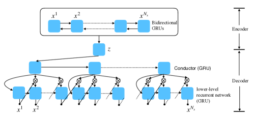
Figure 1: The architecture of FM-Music-​VAE, inspired by the MusicVAE architecture. $\otimes$ denotes vector concatenation.

3.2 Learning Flat Latent Manifolds with Recurrent VAEs

VAEs, including their recurrent version, do not make any assumption on the inferred distances in the latent space. In particular, they do not guarantee that the Euclidean distance in the latent space reflects any similarity between the sequences of the observation space, hence not satisfying our initial desideratum. Therefore, we resort to flattening the latent manifold, i.e., constrain it to act locally as Euclidean space. We define the latent space inferred by the VAE as a Riemannian manifold, as motivated by Chen et al. (2018a). Given a trajectory ${\gamma:[0,1]\rightarrow\mathbb{R}^{N_{\mathbf{z}}}}$ in the latent space, the length in the observation space is $L(\gamma)=\int_{0}^{1}\sqrt{\dot{\gamma}(t)^{T}\,\mathbf{G}\big{(}\gamma(t)\big{)}\>\dot{\gamma}(t)}\,\mathrm{d}t$, where $\mathbf{G}\in\mathbb{R}^{N_{\mathbf{z}}\times N_{\mathbf{z}}}$ is the Riemannian metric tensor, and $\dot{\gamma}(t)$ the derivative. The observation-space distance is defined as the shortest possible path between two data points $D=\min_{\gamma}L(\gamma)$. The trajectory ${\hat{\gamma}=\operatorname*{arg\,min}_{\gamma}L(\gamma)}$ is defined as the (minimising) geodesic. $\gamma$ is projected to the observation space by the decoder of VAEs. With the Jacobian of the decoder with respect to $\mathbf{z}$, the metric tensor is $\mathbf{G}(\mathbf{z})=\mathbf{J}(\mathbf{z})^{T}\mathbf{J}(\mathbf{z})$.

To measure the observation-space distance using simple Euclidean distance in latent space, we have $D\propto\,\|\mathbf{z}(1)-\mathbf{z}(0)\|_{2}$, which indicates that the Riemannian metric tensor is $\mathbf{G}\propto\mathds{1}$. A manifold with this property is defined as flat manifold (Lee, 2006). To learn a model with a flat latent manifold, Chen et al. (2020) presents (i) a flexible prior which allows the model to learn complex latent representations of the data by empirical Bayes; (ii) a regularisation $\mathbf{G}\propto\mathds{1}$; and (iii) data augmentation which enables the model to have the same property in the low data density area.

3.2.1 Hierarchical prior and constrained optimisation

It has been shown that the approximated posterior can be over-regularised when the prior distribution is a standard Normal, which in turn makes the latent representation less informative (Tomczak and Welling, 2018). For instance, a large distance is required for the posteriors between two data points with a large gap, if there is a lack of training data between them. In this case, the model is difficult to be trained by a standard Normal prior. Hence, the motivation to introduce flexible priors arises, such as VampPrior (Tomczak and Welling, 2018) and VHP (Klushyn et al., 2019).

Due to its empirical results and its stable learning, we resort here to the hierarchical prior defined in (Klushyn et al., 2019), $p_{\Theta}(\mathbf{z})=\int\!p_{\Theta}(\mathbf{z}|\mathbf{\zeta})\,p(\mathbf{\zeta})\,\mathrm{d}\mathbf{\zeta}$, where $p(\mathbf{\zeta})$ is the standard normal distribution. Sampling from $q_{\phi}(\mathbf{z}|\mathbf{x})$, we approximate the integral by an importance-weighted (IW) bound Burda et al. (2015). The upper bound on the KL term corresponding to our two stochastic layers is then,

$$\mathbb{E} {}_{p_{\mathcal{D}}(\mathbf{x})}\mathop{\mathbb{KL}}\big{(}q_{\phi}(\mathbf{z}|\mathbf{x})\|\,p(\mathbf{z})\big{)}\leq\mathcal{F}(\phi,\Theta,\Phi)$$

$$\equiv\mathbb{E}_{p_{\mathcal{D}}(\mathbf{x})}\mathop{\mathbb{E}_{q_{\phi}(\mathbf{z}|\mathbf{x})}}\bigg{[}\log q_{\phi}(\mathbf{z}|\mathbf{x})-\mathop{\mathbb{E}_{\mathbf{\zeta}_{1:K}\sim q_{\Phi}(\mathbf{\zeta}|\mathbf{z})}}\Big{[}\log\frac{1}{K}\sum_{i=1}^{K}\frac{p_{\Theta}(\mathbf{z}|\mathbf{\zeta}_{i})\,p(\mathbf{\zeta}_{i})}{q_{\Phi}(\mathbf{\zeta}_{i}|\mathbf{z})}\Big{]}\bigg{]},$$ (2)

where $K$ is the number of importance samples. Based on (Rezende and Viola, 2018), the ELBO is rewritten as the Lagrangian of a constrained optimisation problem:

$$\mathcal{L}_{\text{VHP-VAE}}(\theta,\phi,\Theta,\Phi;\lambda)\equiv\mathcal{F}(\phi,\Theta,\Phi)+\lambda\big{(}\mathop{\mathbb{E}_{p_{\mathcal{D}}(\mathbf{x})}}\mathbb{E}_{q_{\phi}(\mathbf{z}|\mathbf{x})}\big{[}\text{C}_{\theta}(\mathbf{x},\mathbf{z})\big{]}-\kappa^{2}\big{)},$$ (3)

with the optimisation objective $\mathcal{F}(\phi,\Theta,\Phi)$, the inequality constraint $\mathop{\mathbb{E}_{p_{\mathcal{D}}(\mathbf{x})}}\mathbb{E}_{q_{\phi}(\mathbf{z}|\mathbf{x})}\big{[}\text{C}_{\theta}(\mathbf{x},\mathbf{z})\big{]}\leq\kappa^{2}$, and the Lagrange multiplier $\lambda$. $\text{C}_{\theta}(\mathbf{x},\mathbf{z})$ is defined as the reconstruction-error-related term in $-\log p_{\theta}(\mathbf{x}|\mathbf{z})$. Thus, we obtain the following optimisation problem:

$$\min_{\Theta,\Phi}\min_{\theta}\max_{\lambda}\min_{\phi} \>\mathcal{L}_{\text{VHP-VAE}}(\theta,\phi,\Theta,\Phi;\lambda)\quad\text{s.t.}\quad\lambda\geq 0.$$ (4)

3.2.2 Metric tensor regularisation

Regulariser Having defined a constrained optimisation, it becomes straightforward to incorporate the aforementioned regularisation of the Jacobian into the learning scheme to achieve $\mathbf{G}\propto\mathds{1}$ (Chen et al., 2020). The loss function is then,

$$\mathcal{L}_{\text{FM-Music-\!VAE}}(\theta,\phi,\Theta,\Phi;\lambda,\eta,c^{2})=\mathcal{L}_{\text{VHP-VAE}}(\theta,\phi,\Theta,\Phi;\lambda)+\eta\,\mathcal{L}_{\text{FM}}(\theta;c^{2})$$ (5)

with a hyper-parameter, $\eta$, determining the influence of the regularisation, $\mathcal{L}_{\text{FM}}$.

$$\mathcal{L}_{\text{FM}}(\theta;c^{2})=\mathop{\mathbb{E}_{\mathbf{x}_{i,j}\sim p_{\mathcal{D}}(\mathbf{x})}}\mathbb{E}_{\mathbf{z}_{i,j}\sim q_{\phi}(\mathbf{z}|\mathbf{x}_{i,j})}\bigg{[}\big{\|}\mathbf{G}\Big{[}sg\big{(}g(\mathbf{z}_{i},\mathbf{z}_{j})\big{)}\Big{]}-sg(c^{2})\mathds{1}\big{\|}_{2}^{2}\bigg{]},$$ (6)

where $sg$ stands for stop gradient, and $g$ is mixup for exploring the latent space out of the data manifold. The Jacobian is approximated by a stochastic method to improve the computational efficiency. The scaling factor, $c$, is obtained at each batch:

$$c^{2}=\frac{1}{N_{\mathbf{z}}}\,\mathop{\mathbb{E}_{\mathbf{x}_{i,j}\sim p_{\mathcal{D}}(\mathbf{x})}}\mathbb{E}_{\mathbf{z}_{i,j}\sim q_{\phi}(\mathbf{z}|\mathbf{x}_{i,j})}\Big{[}\mathrm{tr}\big{[}\mathbf{G}\big{(}g(\mathbf{z}_{i},\mathbf{z}_{j})\big{)}\big{]}\Big{]}.$$ (7)

Latent space mixup The Jacobian regularisation only affects the vicinity of the training examples, therefore, we use mixup to augment the training data (Zhang et al., 2018). While the original data-augmentation method is applied to the observed data, some previous work (Verma et al., 2019; Chen et al., 2020) extended it to the latent representations. We augment the data by randomly interpolating between two points $\mathbf{z}_{i}$ and $\mathbf{z}_{j}$ in the latent space: $g(\mathbf{z}_{i},\mathbf{z}_{j})=(1-\alpha)\,\mathbf{z}_{i}+\alpha\,\mathbf{z}_{j}$, with $\alpha\sim U(-\alpha_{0},1+\alpha_{0})$. To compute more efficiently, we obtain $\mathbf{z}_{i}$ and $\mathbf{z}_{j}$ by shuffling a batch of $\mathbf{z}$. In order to take into account the outer edge of the data manifold, we have $\alpha_{0}>0$. With the metric tensor regularisation in the entire latent space enclosed by the data manifold, the decoder $f(\mathbf{z})$ is distance-preserving. Given the distance in the observation space $D_{\mathbf{x}}$, and in the latent space $D_{\mathbf{z}}$, we obtain $D_{\mathbf{x}}(f(\mathbf{z}_{i}),f(\mathbf{z}_{j}))\approx c\,D_{\mathbf{z}}(\mathbf{z}_{i},\mathbf{z}_{j})$.

Jacobian approximation To improve the computational efficiency, we approximate the Jacobian with a first-order Taylor expansion (Rifai et al., 2011; Chen et al., 2020). Alternatively, we use a different sampling-based approximation that scales gracefully (Nesterov and Spokoiny, 2017),

$$\mathbf{J}(\mathbf{z})=\frac{1}{\mu}E_{\mathbf{u}}\big{(}f(\mathbf{z}+\mu\mathbf{u})\mathbf{u}\big{)}\equiv\frac{1}{\mu}E_{\mathbf{u}}\big{(}[f(\mathbf{z}+\mu\mathbf{u})-f(\mathbf{z})]\mathbf{u}\big{)},$$ (8)

where $\mathbf{u}\in\mathbb{R}^{N_{\mathbf{z}}}$ is a normally distributed Gaussian vector and $\mu$ is a bound. The computation of eq. 8 depends on the sample size used to approximate the expectation of $\mathbf{u}$. Therefore, for small $N_{\mathbf{z}}$, the first-order Taylor expansion is employed, while we use eq. 8 for large $N_{\mathbf{z}}$.

4 Experiments and live deployment

To assess the quality of our latent representation, we measure the smoothness and quality of the interpolation and explore how musical attributes are projected into the latent space. Throughout the experiments, we obtain the hyper parameters of the models via random search. Generated audio samples are available online. We compare our approach with MusicVAE (Roberts et al., 2018), as the SOTA model for interpolating music data.Quantitative evaluation is done on three music datasets.

Drum dataset We evaluate our model on a drum/groove dataset (Gillick et al., 2019) with two variations consisting in two- and four-bar sequences respectively. Each bar consists of 16 time steps. It is recorded on a Roland TD-$11^{2}$ electronic drum kit and we map the kit to nine categories. In each time step, the data (MIDI notes) consists of binary-valued hits (the drum score for nine instruments), discrete-valued velocity (how strong the drums are struck), and continuous-valued offsets (indicating the micro-timing of how soon/late the note is played). Since the splits of the training, validation and testing in (Gillick et al., 2019) easily cause overfitting and early stopping, we randomly re-split the training and validation.

Piano and cello datasets We obtain the piano dataset from Ryan’s Mammoth of the music21 toolkit (Cuthbert and Ariza, 2010) and the cello dataset from the Bach Cello Suites (www.kunstderfuge.com). Each dataset is augmented by pitch shifting. Therefore, the note distribution covers the full range of the 88 piano keys. One sequence contains 4 bars, i.e., 64 time steps in total and each time step has 90 dimensions consisting of 88 ‘note-on’, one ‘note-off’, and one ‘rest’ (Roberts et al., 2018). For each dataset, we randomly split the data into 80%, 10% and 10%, respectively for training, validation and testing in sections 4.1 and 4.3. The dataset splitting is different for interpolation quality evaluation in section 4.2.

4.1 Evaluating the interpolations’ smoothness

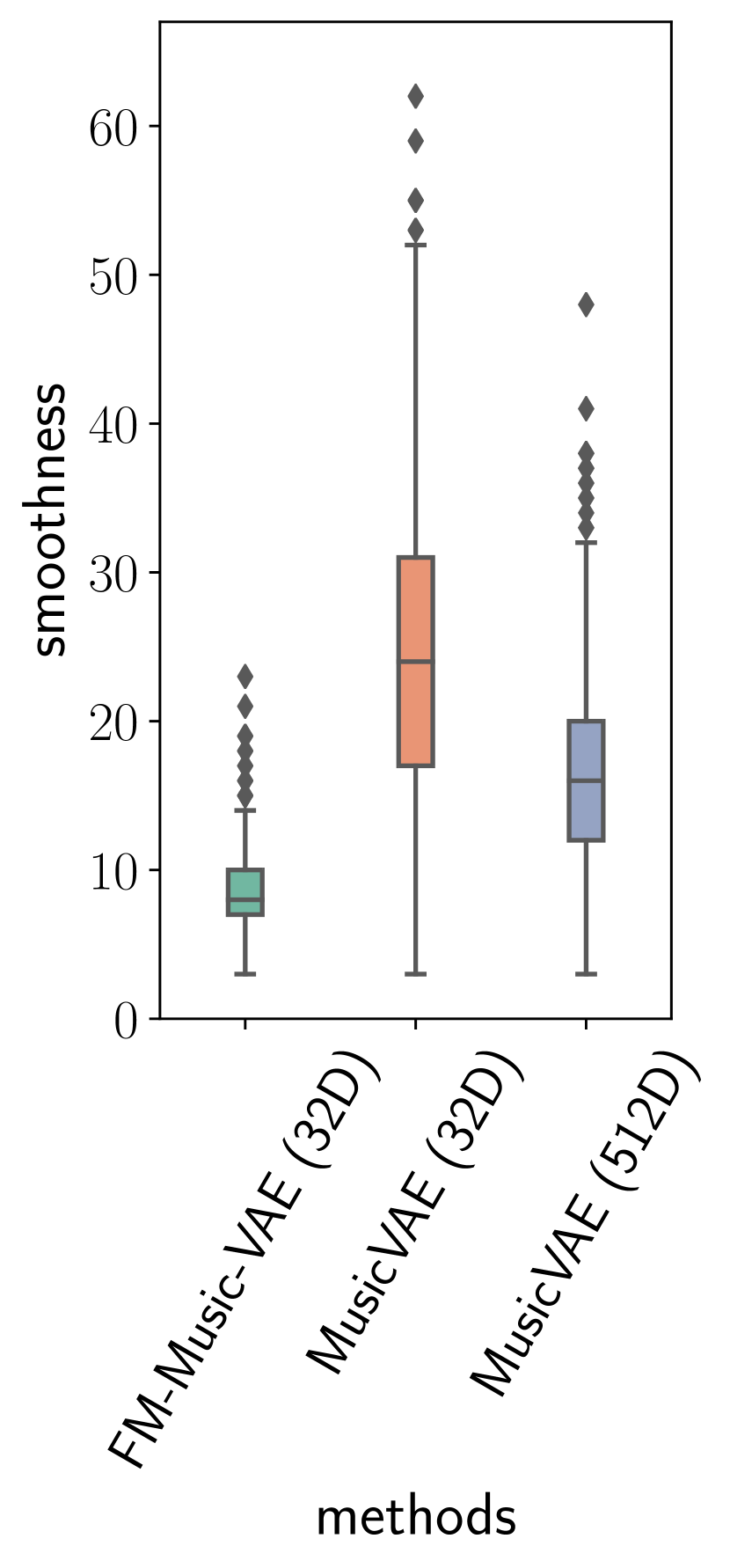
(a)

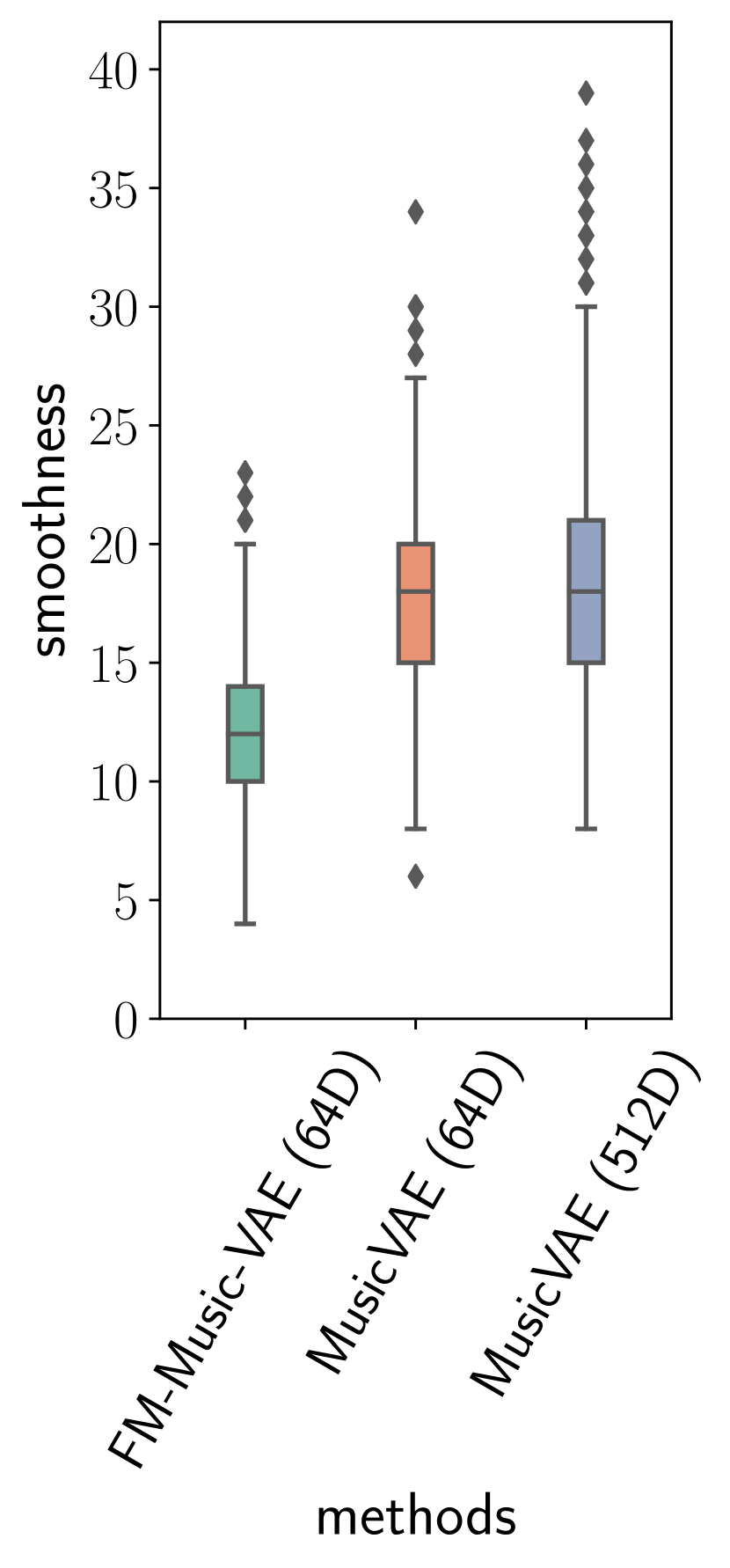
(b)

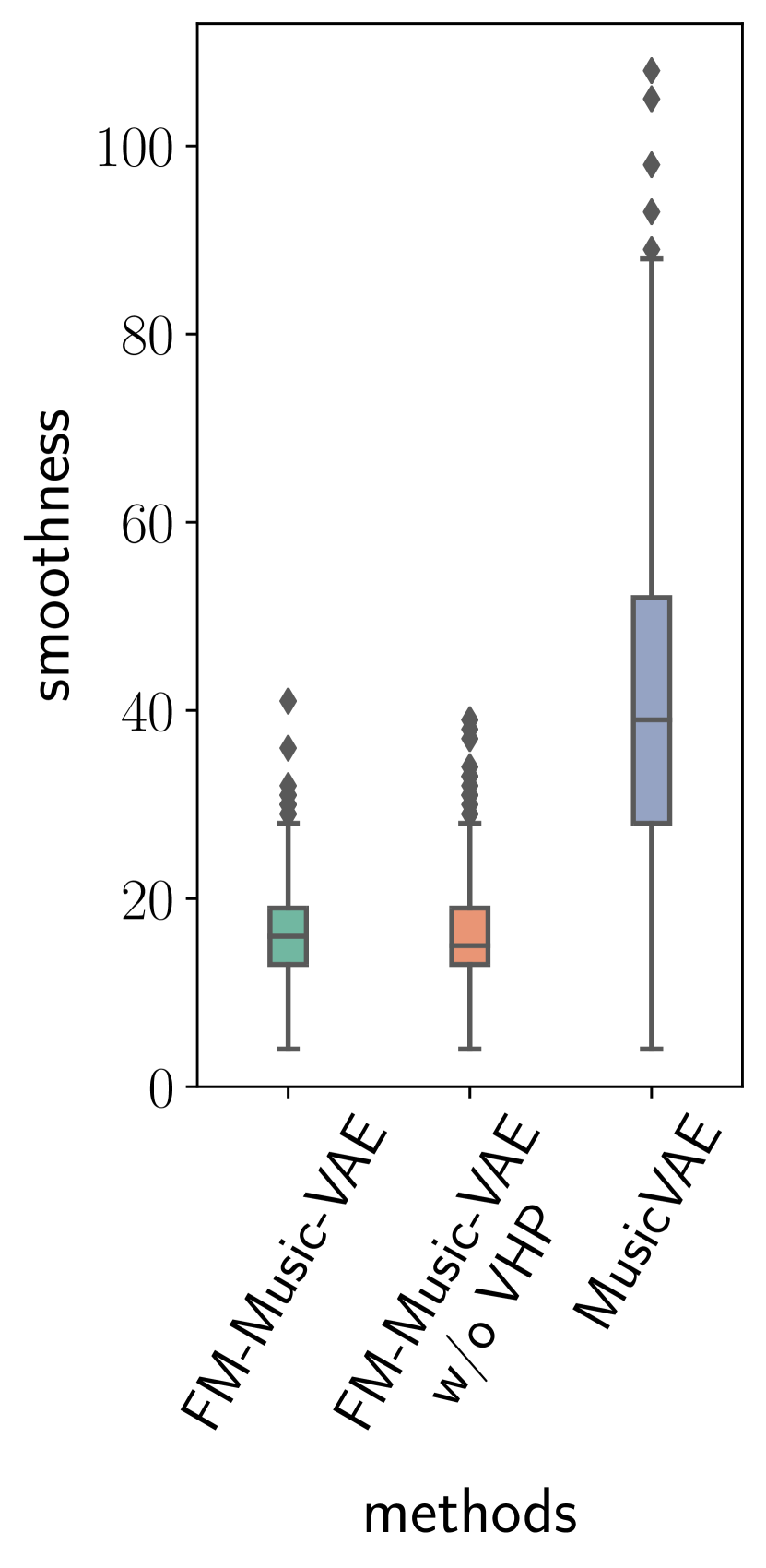
(c)

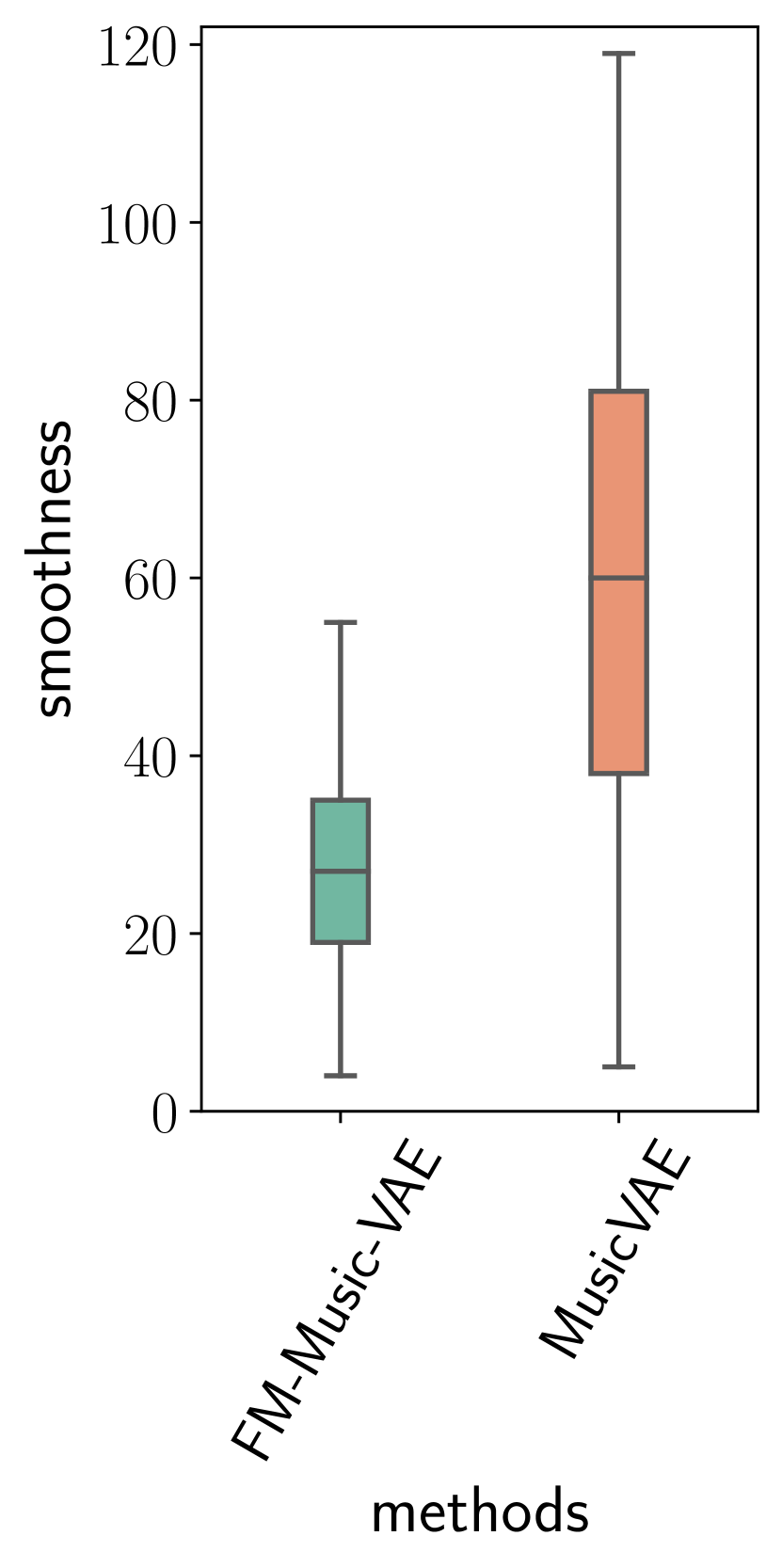
(d)

Figure 2: A comparison of the smoothness of FM-Music-​VAE and MusicVAE. The brackets indicate the dimensionality of the latent space. (a) and (b) are drum and piano data, respectively, with two bars and various latent dimensions. (c) drum data with four bars and 32 latent dimensions. (d) cello data with four bars and 64 latent dimensions.

We take the hits and on-notes for the drum and piano datasets respectively to compute smoothness. Since they are binary data, we define the smoothness of a sequence as $\max_{t\in[0,1\dots,N-1]}D_{\mathrm{h}}(\mathbf{x}_{t},\mathbf{x}_{t+1})$, where $D_{\mathrm{h}}$ represents Hamming distance, and $\mathbf{x}_{t}$ is a sequence at step $t$ of the interpolation. Figure 2 shows the smoothness of 1 000 pairs and 20 interpolated points. Interpolated samples are shown in fig. 4. With MusicVAE, the smoothness improves with a sufficiently large number of dimensions in the latent space, however, our approach is able to get overall better smoothness with a significantly lower-dimensional latent space. In this experiment, MusicVAE uses linear interpolation instead of the Slerp for the smoothness evaluation, since we expect to explore the whole latent space for more creativity instead of only interpolating between two points and generate data similar to the training dataset.

4.2 Evaluating the interpolations’ quality

Evaluating the quality of the interpolations via human ratings is subject to a substantial bias. Hence, we quantify the quality of the interpolation by measuring some generalisation properties in between the training data points, namely, the velocity and offset for the drum data, the pitch for the piano, and the notes density for both. All of these properties are part of the input data except for the notes density which we manually count for each two bars. Using the middle decile or the middle 50 percentile as a ground truth of testing datasets, we obtain the samples between the other two ends (training and validation datasets) of the distribution for each of the aforementioned properties. The results for each property are summarised in table 1. Since the piano and cello datasets are one-hot encoded, the reconstruction error rate $\delta$ is reported for the whole frame, i.e., $\delta={N_{f}}/{N_{s}}$, with $N_{f}$ being the number of the incorrectly reconstructed frames in a sequence. On the other hand, the error rate for the drum data is computed on a per-beat level for the density attribute, i.e., $\delta={N_{fp}}/({N_{x}N_{s}})$, where $N_{fp}$ is the number of wrongly predicted beats in a sequence. As for the velocity and offset, we report the mean square errors (MSEs) per beat. All the reported numbers, the mean and standard deviation, are evaluated over the test datasets.

Table 1: Evaluating the quality of the interpolation. The bold font indicates the best result. The models of the drum datasets are 32D latent space, while of the piano and cello datasets are 64D latent space. The first column shows the dataset and the percentile used for test datasets.

dataset (percentile)	model	density	velocity	offset
Drum, four bars	FM-Music-​VAE	0.039 $\pm$ 0.023	0.0116 $\pm$ 0.0080	0.0039 $\pm$ 0.0022
(10%)	MusicVAE	0.051 $\pm$ 0.031	0.0151 $\pm$ 0.0123	0.0042 $\pm$ 0.0024
Drum, four bars	FM-Music-​VAE	0.064 $\pm$ 0.030	0.0195 $\pm$ 0.0116	0.0050 $\pm$ 0.0027
(50%)	MusicVAE	0.094 $\pm$ 0.037	0.0286 $\pm$ 0.0163	0.0058 $\pm$ 0.0031
dataset (percentile)	model	density	pitch
Piano, two bars	FM-Music-​VAE	0.195 $\pm$ 0.093	0.165 $\pm$ 0.099
(50%)	MusicVAE	0.234 $\pm$ 0.222	0.431 $\pm$ 0.088
Cello, four bars	FM-Music-​VAE	0.145 $\pm$ 0.183	0.117 $\pm$ 0.165
(50%)	MusicVAE	0.616 $\pm$ 0.194	0.560 $\pm$ 0.211

4.3 Exploiting the structure of the latent space with attribute vectors

Table 2: The correlation of the attribute and the latent space (Pearson’s correlation coefficient). The bold font represents the best result.

dataset	model	density	velocity	offset	pitch
Drum, two bars	FM-Music-​VAE (32D)	0.89	0.84	0.69	-
	MusicVAE (32D)	0.50	0.27	0.21	-
	MusicVAE (512D)	0.74	0.56	0.52	-
Drum, four bars	FM-Music-​VAE (32D)	0.89	0.87	0.72	-
	FM-Music-​VAE w/o VHP (32D)	0.87	0.88	0.60	-
	MusicVAE (32D)	0.73	0.31	0.59	-
Piano, two bars	FM-Music-​VAE (64D)	0.89	-	-	0.77
	MusicVAE (64D)	0.37	-	-	0.42
	MusicVAE (512D)	0.48	-	-	0.50
Cello, four bars	FM-Music-​VAE (64D)	0.91	-	-	0.81
	MusicVAE (64D)	0.79	-	-	0.60

The structure of the latent spaces can be exploited using attribute vectors (Roberts et al., 2018; White, 2016). In particular, we exploit the density, velocity and offset attributes in the drum dataset, as well as the density and pitch attributes in the piano dataset. The density attribute is computed by summing the hits (drum) or on-notes (piano) over two bars. The velocity/offset/pitch attributes are the mean over the velocities/offsets/pitches of each sequence where notes exist.

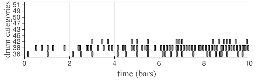
(a) FM-Music-​VAE (32D)

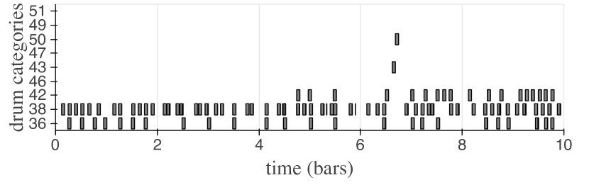
(b) MusicVAE (32D)

Figure 3: Density vector. The middle data point (two bars) of each subfigure is from the datasets. From the left to the right directions are the attribute vectors with the scale factor from $-1$ to 1.

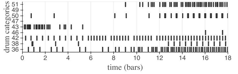
(c) FM-Music-​VAE (32D)

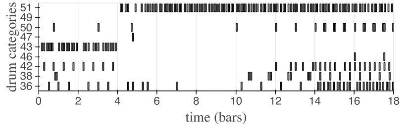
(d) MusicVAE (32D)

Figure 4: A comparison of music interpolation. Given the starting and ending sequences, seven points are linearly interpolated in the latent space.

5 000 samples are selected to compute the highest and lowest 25% percentile for each attribute, and the mean positions are computed accordingly in these regions of the latent spaces. The direction is then calculated based on the centroids. Based on a data point in the latent space, previous work (Roberts et al., 2018) subtracts or adds a vector to evaluate the features. Motivated by the continuous nature of music (in contrast to discrete image features such as wearing or not wearing glasses), we instead randomly scale the vector length with a scale factor in the range of $[-1,1]$, and then compute the linear correlation between the vector length in the latent space and attributes in the observation space. If the data point with the scaled attribute vector in the latent space exceeds the range of any axis, the corresponding sample is discarded. In the end, 5 000 samples are used to calculate the correlation. Table 2 indicates that the latent space of the proposed approach is more structured. The 2-tailed p-values are zero or close to zero, so they are not shown in the tables. Figure 4 illustrates an example of moving in the latent space along the density vector. The FM-Music-​VAE retains the patterns of the illustrated data, while the density changes.

Ablation study Motivating our design choices, we conduct an ablation study in order to assess the effect of the hierarchical prior described in section 3.2.1. Table 2 shows that while FM-Music-​VAE with a standard Normal prior does improve over the state-of-the-art, adding the hierarchical prior further improves the performance. Hence, the rest of the experiments are conducted with the full model.

4.4 Drummer-model interactive deployment

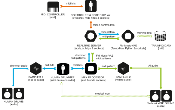
Figure 5: The architecture of the jam session.

The final test of FM-Music-​VAE was in a live artistic event. During the session, a professional drummer interacted with our model by playing two bars of drum music, to which our model ‘responded’ with another generated two-bars drum sequence. Once received, the drummer’s playing was mapped into a point in the latent space. Using this point as the centre of a Gaussian distribution, a second point was then sampled and decoded into a drum sequence that the drummer could listen to – and hopefully be inspired by. The back-and-forth interplay lasted for about ten minutes. While playing, the drummer was also able to visualise the three-dimensional embedding of his own playing as well as that of the model’s generations. The set of embedded points were also visually linked to reflect their occurrence in time, hence forming the two ‘trajectories’ of the two players in a three-dimensional space. The goal was to let the drummer try to ‘influence’ the direction the model was taking, a task that is only feasible if the latent representations can be properly interpreted.

To facilitate the musical dialog between a human drummer and the FM-Music-​VAE, the infrastructure was built up around realtime socket connections. The latency, introduced by processing of the data, was overcome by working in bars of notes instead of sending over individual hits. The drummer played on a midi drum set and the individual notes were captured by a Max application and sequenced into two bars. The bars were sent over to a central server which acted as a broker between the AI model and the human drummer. The forwarded bars were processed by the model into two response-bars and sent back to the Max application in reverse route. For both human drummer and AI a separate sampler was used to convert the midi into hearable audio. Figure 5 depicts the architecture deployed during the live session.

Although the performance itself excludes any scientific pretension, we argue that the deployment of our model in this context brings value on three different fronts. First, it shows that our latent-variable model can be used for interpretability purposes, even by a non-machine-learning practitioner, as it exhibits meaningful distances. We also make the point that deploying models is valuable in itself, even in the context of scientific research, as it is anchored in real needs (Wagstaff, 2012). Finally, contributing to a novel musical experience in which an artist has the possibility to explore music both audibly and visually constitutes an artistic value. An excerpt of the performance video is available online.

5 Conclusion and future work

We presented FM-Music-​VAE, a theoretically-motivated approach to live interaction with a human musician while learning a high-level music representation. Our method in effect learns a distance metric for sequence data that allows for smooth and meaningful linear interpolations. Using drums and piano datasets, we experimentally demonstrated that our principled constrained optimisation scheme properly regularises the decoder and thus yields realistic music sequences. Finally, the interactive music session between the model and a drummer illustrates that the proposed approach is able to be intuitively used by a human, although a more thorough and scientific study is needed to support this initial observation. In the future, using high-level control in latent space, e.g. through, reinforcement learning, for generating longer musical sequences would be a natural follow-up.

Appendix A Appendix

A.1 Interpolation of the drum dataset

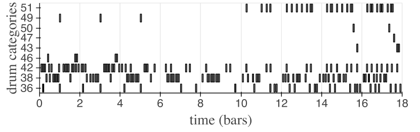
(a) FM-Music-​VAE

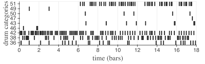
(b) MusicVAE (32D)

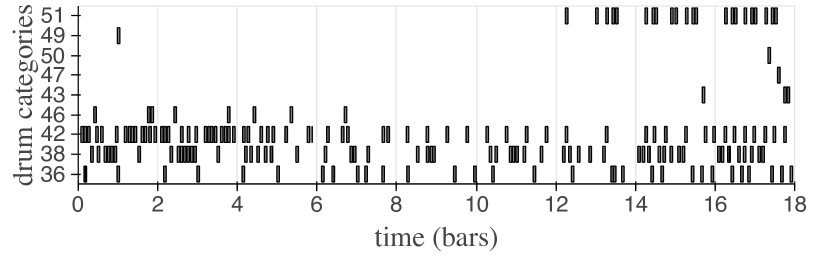
(c) MusicVAE (512D)

Figure 6: Drum interpolation. See fig. 4 for more details.

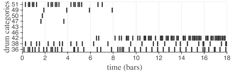
(a) FM-Music-​VAE

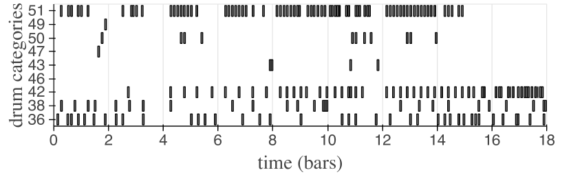
(b) MusicVAE (32D)

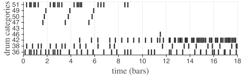
(c) MusicVAE (512D)

Figure 7: Drum interpolation. See fig. 4 for more details.

A.2 Drum density attribute

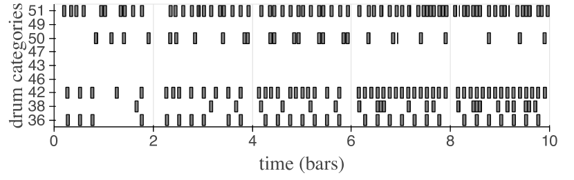
(a) FM-Music-​VAE

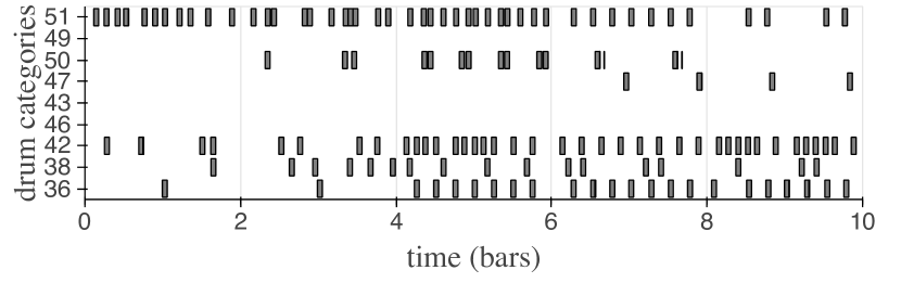
(b) MusicVAE (32D)

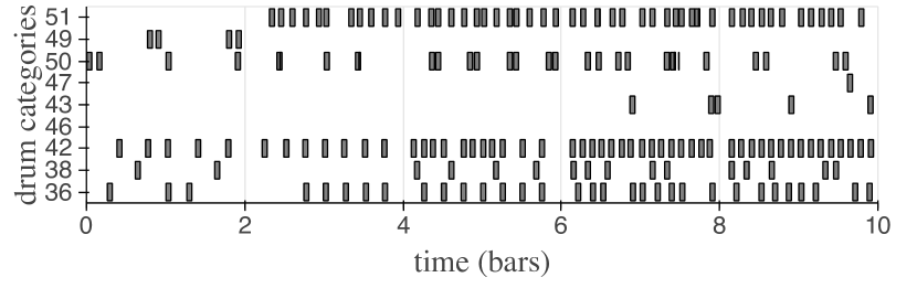
(c) MusicVAE (512D)

Figure 8: Drum density attribute. See fig. 4 for more details.

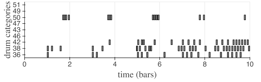
(a) FM-Music-​VAE

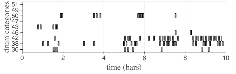
(b) MusicVAE (32D)

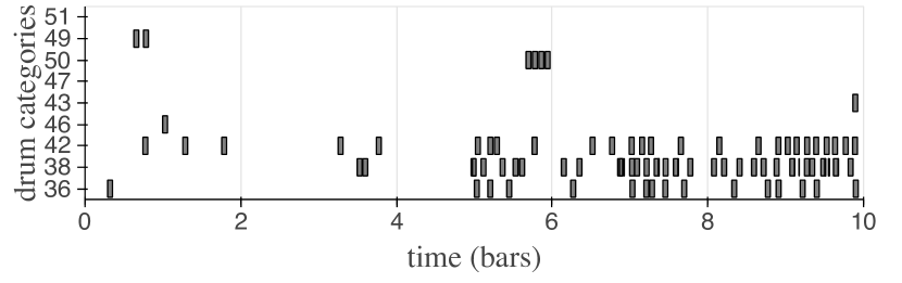
(c) MusicVAE (512D)

Figure 9: Drum density attribute. See fig. 4 for more details.

A.3 Drum velocity attribute

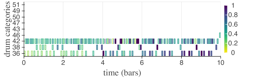
(a) FM-Music-​VAE

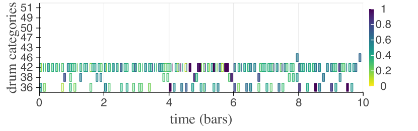
(b) MusicVAE (32D)

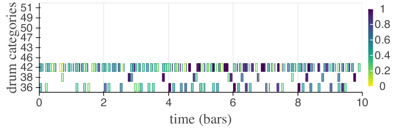
(c) MusicVAE (512D)

Figure 10: Drum velocity distribute. The colour represents the velocity. See fig. 4 for more details.

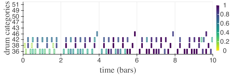
(a) FM-Music-​VAE

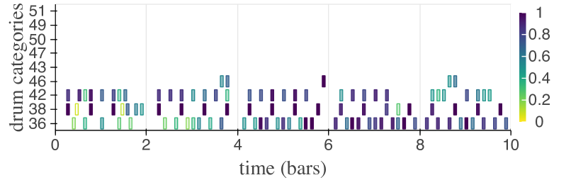
(b) MusicVAE (32D)

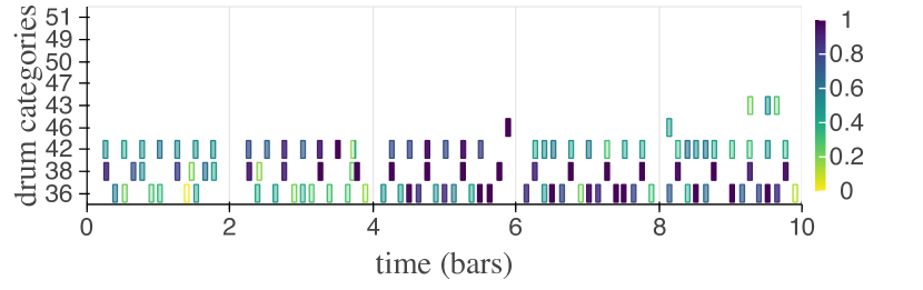
(c) MusicVAE (512D)

Figure 11: Drum velocity attribute. The colour represents the velocity. See fig. 4 for more details.

A.4 Interpolation of the piano dataset

(a) FM-Music-​VAE

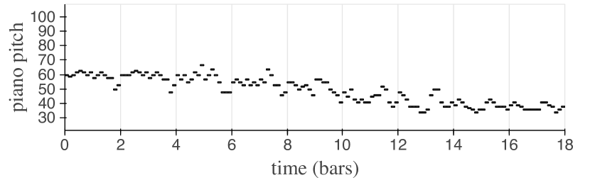
(b) MusicVAE (32D)

(c) MusicVAE (512D)

Figure 12: Piano interpolation. See fig. 4 for more details.

(a) FM-Music-​VAE

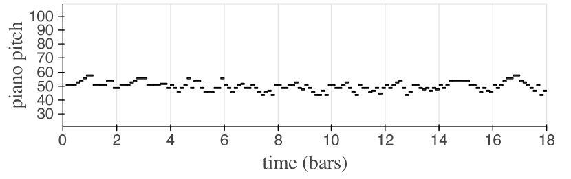
(b) MusicVAE (32D)

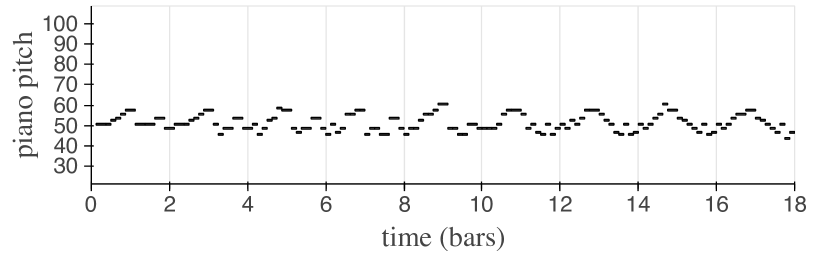
(c) MusicVAE (512D)

Figure 13: Piano interpolation. See fig. 4 for more details.

A.5 Piano density attribute

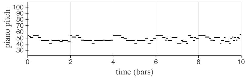
(a) FM-Music-​VAE

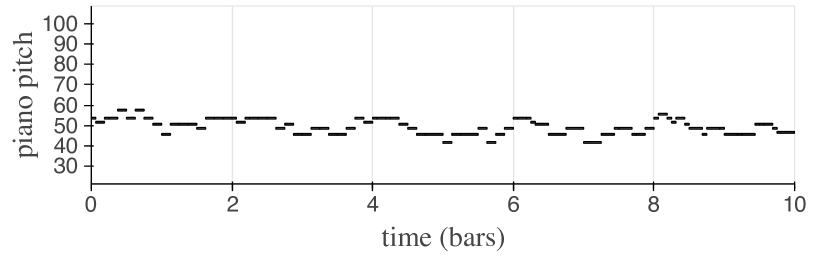
(b) MusicVAE (32D)

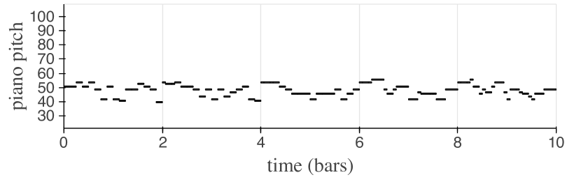
(c) MusicVAE (512D)

Figure 14: Piano density attribute. See fig. 4 for more details.

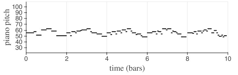
(a) FM-Music-​VAE

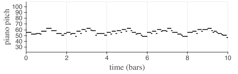
(b) MusicVAE (32D)

(c) MusicVAE (512D)

Figure 15: Piano density attribute. See fig. 4 for more details.

A.6 Model Architectures

Table 3: Model architectures. FC is fully-connected layers. $\nu$ is defined in [Klushyn et al., 2019]. The models were trained on a single 16-G GPU.

Dataset	Optimiser	Architecture
Drum(four bars)	Adam	Input	64$\times$27
	5$e$-4 w/ decay	Latents	32
		$q_{\phi}(\mathbf{z}|\mathbf{x})$	BiGRU 1024, 1024.
		$p_{\theta}(\mathbf{x}|\mathbf{z})$	Conductor 512, GRU 512, 512.
		$q_{\Phi}(\mathbf{\zeta}|\mathbf{z})$	FC 256, 256, ReLU activation.
		$p_{\Theta}(\mathbf{z}|\mathbf{\zeta})$	FC 256, 256, ReLU activation.
		Others	$\kappa$ = 0.15, $\nu$ = 1, $K$ = 16, $\eta=2500$.
Piano	Adam	Input	32$\times$90
	5$e$-4 w/ decay	Latents	64
		$q_{\phi}(\mathbf{z}|\mathbf{x})$	BiGRU 1024, 1024.
		$p_{\theta}(\mathbf{x}|\mathbf{z})$	Conductor 512, GRU 512, 512.
		$q_{\Phi}(\mathbf{\zeta}|\mathbf{z})$	FC 256, 256, ReLU activation.
		$p_{\Theta}(\mathbf{z}|\mathbf{\zeta})$	FC 256, 256, ReLU activation.
		Others	$\kappa$ = 0.03, $\nu$ = 1, $K$ = 8, $\eta=2000$.
Cello	Adam	Input	64$\times$90
	5$e$-4 w/ decay	Latents	64
		$q_{\phi}(\mathbf{z}|\mathbf{x})$	BiGRU 1024, 1024.
		$p_{\theta}(\mathbf{x}|\mathbf{z})$	Conductor 512, GRU 512, 512.
		$q_{\Phi}(\mathbf{\zeta}|\mathbf{z})$	FC 256, 256, ReLU activation.
		$p_{\Theta}(\mathbf{z}|\mathbf{\zeta})$	FC 256, 256, ReLU activation.
		Others	$\kappa$ = 0.06, $\nu$ = 1, $K$ = 8, $\eta=2000$.

A.7 Drum categories

Table 4: Drum categories. The mapping from the pitch to the nine drum categories. Gillick et al. [2019] shows more details of the mapping.

Drum Category	Pitch
Bass	36
Snare	38
High Tom	50
Low-Mid Tom	47
High Floor Tom	43
Open Hi-Hat	46
Closed Hi-Hat	42
Crash Cymbal	49
Ride Cymbal	51

References

- Alemi et al. [2018] Alexander A Alemi, Ben Poole, Ian Fischer, Joshua V Dillon, Rif A Saurous, and Kevin Murphy. Fixing a broken ELBO. ICML, 2018.
- Arvanitidis et al. [2018] Georgios Arvanitidis, Lars Kai Hansen, and Søren Hauberg. Latent space oddity: on the curvature of deep generative models. In ICLR, 2018.
- Bayer and Osendorfer [2014] Justin Bayer and Christian Osendorfer. Learning stochastic recurrent networks. arXiv preprint arXiv:1411.7610, 2014.
- Bayer et al. [2012] Justin Bayer, Christian Osendorfer, and Patrick van der Smagt. Learning sequence neighbourhood metrics. In ICANN, pages 531–538. Springer, 2012.
- Berthelot et al. [2019] David Berthelot, Colin Raffel, Aurko Roy, and Ian Goodfellow. Understanding and improving interpolation in autoencoders via an adversarial regularizer. In ICLR, 2019.
- Bowman et al. [2016] Samuel R. Bowman, Luke Vilnis, Oriol Vinyals, Andrew Dai, Rafal Jozefowicz, and Samy Bengio. Generating sentences from a continuous space. In CoNLL, pages 10–21, 2016.
- Burda et al. [2015] Yuri Burda, Roger B. Grosse, and Ruslan Salakhutdinov. Importance weighted autoencoders. CoRR, abs/1509.00519, 2015.
- Chen et al. [2018a] Nutan Chen, Alexej Klushyn, Richard Kurle, Xueyan Jiang, Justin Bayer, and Patrick van der Smagt. Metrics for deep generative models. In AISTATS, pages 1540–1550, 2018.
- Chen et al. [2018b] Nutan Chen, Alexej Klushyn, Alexandros Paraschos, Djalel Benbouzid, and Patrick van der Smagt. Active learning based on data uncertainty and model sensitivity. IEEE/RSJ IROS, 2018.
- Chen et al. [2019] Nutan Chen, Francesco Ferroni, Alexej Klushyn, Alexandros Paraschos, Justin Bayer, and Patrick van der Smagt. Fast approximate geodesics for deep generative models. In ICANN, pages 554–566. Springer, 2019.
- Chen et al. [2020] Nutan Chen, Alexej Klushyn, Francesco Ferroni, Justin Bayer, and Patrick van der Smagt. Learning flat latent manifolds with vaes. In ICML, 2020.
- Cho et al. [2014] Kyunghyun Cho, Bart Van Merriënboer, Dzmitry Bahdanau, and Yoshua Bengio. On the properties of neural machine translation: Encoder-decoder approaches. arXiv preprint arXiv:1409.1259, 2014.
- Chung et al. [2014] Junyoung Chung, Caglar Gulcehre, KyungHyun Cho, and Yoshua Bengio. Empirical evaluation of gated recurrent neural networks on sequence modeling. NIPS Workshop on Deep Learning, 2014.
- Cuthbert and Ariza [2010] Michael Scott Cuthbert and Christopher Ariza. music21: A toolkit for computer-aided musicology and symbolic music data. International Society for Music Information Retrieval, 2010.
- Engel et al. [2018] Jesse Engel, Matthew Hoffman, and Adam Roberts. Latent constraints: Learning to generate conditionally from unconditional generative models. ICLR, 2018.
- Fraccaro et al. [2016] Marco Fraccaro, Søren Kaae Sønderby, Ulrich Paquet, and Ole Winther. Sequential neural models with stochastic layers. NIPS, 2016.
- Garreau et al. [2014] Damien Garreau, Rémi Lajugie, Sylvain Arlot, and Francis Bach. Metric learning for temporal sequence alignment. NIPS, 2014.
- Gillick et al. [2019] Jon Gillick, Adam Roberts, Jesse H. Engel, Douglas Eck, and David Bamman. Learning to groove with inverse sequence transformations. In ICML, 2019.
- Ha and Eck [2018] David Ha and Douglas Eck. A neural representation of sketch drawings. In ICLR, 2018.
- Hadjeres et al. [2017] Gaëtan Hadjeres, Frank Nielsen, and François Pachet. Glsr-vae: Geodesic latent space regularization for variational autoencoder architectures. In SSCI, pages 1–7. IEEE, 2017.
- Hochreiter and Schmidhuber [1997] Sepp Hochreiter and Jürgen Schmidhuber. Long short-term memory. Neural computation, 9(8):1735–1780, 1997.
- Karl et al. [2017] Maximilian Karl, Maximilian Soelch, Justin Bayer, and Patrick Van der Smagt. Deep variational bayes filters: Unsupervised learning of state space models from raw data. ICLR, 2017.
- Kingma and Welling [2014] Diederik P. Kingma and Max Welling. Auto-encoding variational Bayes. ICLR, 2014.
- Kingma et al. [2016] Durk P Kingma, Tim Salimans, Rafal Jozefowicz, Xi Chen, Ilya Sutskever, and Max Welling. Improved variational inference with inverse autoregressive flow. In NIPS, volume 29, 2016.
- Klushyn et al. [2019] Alexej Klushyn, Nutan Chen, Richard Kurle, Botond Cseke, and Patrick van der Smagt. Learning hierarchical priors in VAEs. NeurIPS, 2019.
- Knees and Schedl [2013] Peter Knees and Markus Schedl. A survey of music similarity and recommendation from music context data. TOMM, 2013.
- Krishnan et al. [2015] Rahul G Krishnan, Uri Shalit, and David Sontag. Deep kalman filters. arXiv, 2015.
- Kumar and Poole [2020] Abhishek Kumar and Ben Poole. On implicit regularization in -vaes. In ICML, 2020.
- Lee [2006] John M Lee. Riemannian manifolds: an introduction to curvature, volume 176. Springer Science & Business Media, 2006.
- Mei et al. [2015] Jiangyuan Mei, Meizhu Liu, Yuan-Fang Wang, and Huijun Gao. Learning a mahalanobis distance-based dynamic time warping measure for multivariate time series classification. IEEE Trans Cybern, 46, 2015.
- Müller [2007] Meinard Müller. Dynamic time warping. Information retrieval for music and motion, pages 69–84, 2007.
- Nesterov and Spokoiny [2017] Yurii Nesterov and Vladimir Spokoiny. Random gradient-free minimization of convex functions. FoCM, 17(2):527–566, 2017.
- Pati and Lerch [2021] Ashis Pati and Alexander Lerch. Attribute-based regularization of latent spaces for variational auto-encoders. Neural Computing and Applications, 33(9):4429–4444, 2021.
- Rezende and Viola [2018] Danilo Jimenez Rezende and Fabio Viola. Taming VAEs. arXiv, 2018.
- Rezende et al. [2014] Danilo Jimenez Rezende, Shakir Mohamed, and Daan Wierstra. Stochastic backpropagation and approximate inference in deep generative models. In ICML, volume 32, pages 1278–1286, 2014.
- Rifai et al. [2011] Salah Rifai, Grégoire Mesnil, Pascal Vincent, Xavier Muller, Yoshua Bengio, Yann Dauphin, and Xavier Glorot. Higher order contractive auto-encoder. In ECML-PKDD, pages 645–660. Springer, 2011.
- Roberts et al. [2018] Adam Roberts, Jesse Engel, Colin Raffel, Curtis Hawthorne, and Douglas Eck. A hierarchical latent vector model for learning long-term structure in music. In ICML, volume 80, pages 4364–4373, 2018.
- Schuster and Paliwal [1997] Mike Schuster and Kuldip K Paliwal. Bidirectional recurrent neural networks. IEEE Trans. on Signal Processing, 45(11):2673–2681, 1997.
- Su and Wu [2019] Bing Su and Ying Wu. Learning distance for sequences by learning a ground metric. In ICML, 2019.
- Tomczak and Welling [2018] Jakub M. Tomczak and Max Welling. VAE with a vampprior. In AISTATS, 2018.
- Verma et al. [2019] Vikas Verma, Alex Lamb, Christopher Beckham, Amir Najafi, Ioannis Mitliagkas, David Lopez-Paz, and Yoshua Bengio. Manifold mixup: Better representations by interpolating hidden states. In ICML, volume 97, pages 6438–6447, 2019.
- Volk et al. [2016] Anja Volk, Elaine Chew, Elizabeth Hellmuth Margulis, and Christina Anagnostopoulou. Music similarity: Concepts, cognition and computation. JNMR, 45(3):207–209, 2016.
- Wagstaff [2012] Kiri Wagstaff. Machine learning that matters. ICML, 2012.
- Wang et al. [2020] Ziyu Wang, Yiyi Zhang, Yixiao Zhang, Junyan Jiang, Ruihan Yang, Junbo Zhao, and Gus Xia. Pianotree vae: Structured representation learning for polyphonic music. ISMIR, 2020.
- White [2016] Tom White. Sampling generative networks. arXiv preprint arXiv:1609.04468, 2016.
- Yang et al. [2019] Ruihan Yang, Tianyao Chen, Yiyi Zhang, and Gus Xia. Inspecting and interacting with meaningful music representations using vae. arXiv, 2019.
- Zhang et al. [2018] Hongyi Zhang, Moustapha Cisse, Yann N. Dauphin, and David Lopez-Paz. mixup: Beyond empirical risk minimization. ICLR, 2018.