Noise-assisted and monitoring-enhanced quantum bath tagging

Abstract

We analyze the capability of discriminating the statistical nature of a thermal bath by exploiting the interaction with an additional environment. We first shows that, at difference with the standard scenario where the additional environment is not present, the modified evolution induced by the mere presence of the extra bath allows to improve the discrimination task. We then also consider the possibility of continuously monitoring the additional environment and we discuss in detail how to obtain improved performances in the discrimination by considering different kinds of interaction, i.e. different jump operators, and different monitoring strategies corresponding to continuous homodyne and photo-detection. Our strategy can be in principle implemented in a circuit QED setup and paves the way to further developments of quantum probing via continuous monitoring.

I Introduction

In quantum metrology and quantum sensing Giovannetti et al. (2006, 2011); Paris (2009); Demkowicz-Dobrzański et al. (2015); Degen et al. (2017); Pirandola et al. (2018) a quantum probe is any physical system that allows for the recovery an unknown classical parameter that has been “attached” to its state via some dedicated dynamical process. For instance quantum probes have been used to estimate parameters related either to their Hamiltonian (e.g. a frequency or a coupling constant) or to their unitary evolution (say a dynamical phase accumulated while moving along a certain trajectory). Quantum probes have also been exploited in order to reconstruct the properties of the surrounding environment Mehboudi et al. (2019); examples are protocols of quantum thermometry Stace (2010); Brunelli et al. (2011); Correa et al. (2015); Paris (2015); De Pasquale et al. (2016, 2017); Campbell et al. (2018); Kiilerich et al. (2018); Cavina et al. (2018); Razavian et al. (2019) or aimed to characterize the spectrum of the environment itself Benedetti et al. (2018); Bina et al. (2018). More recently it has been proposed to use a quantum probe to discriminate between thermal baths characterized by different thermal Candeloro and Paris (2021) or statistical Farina et al. (2019); Gianani et al. (2020) properties. In particular in the latter scenario, a quantum probe $S$ is exploited to determine whether the the thermal bath $E$ obeys to Bosonic or Fermionic statistics, a task which hereafter will be referred to as Quantum Bath Tagging (QBT). In such scheme $S$ is let to weakly interact with $E$ for some time $t$ and then measured using optimal detection procedures identified by solving the associated quantum hypothesis testing problem Helstrom (1969). To improve further the discrimination performances reported in Farina et al. (2019); Gianani et al. (2020) and to refer more closely to realistic experimental setups, we consider here the possibility that while coupled with $E$, the probe $S$ could be made interact also with a second auxiliary bath $A$ which, at variance with what happens with $E$, is assumed to have known statistical and thermodynamical properties (specifically we shall take $A$ to be a, zero-temperature, multi-mode electromagnetic (e.m.) field). The role of such an extra environment is twofold: on one hand, the presence of $A$ is used as a way to positively interfere with the $S$-$E$ coupling in an effort to increase the distinguishability among the quantum trajectories associated with the two hypothesis of the problem; on the second hand, $A$ is employed to set up an indirect, continuous monitoring of the evolution of $S$, hence allowing us to acquire information about $E$ in real time and not just at the end of the interaction interval. Continuous monitoring of quantum systems Wiseman and Milburn (2009); Jacobs and Steck (2006) has indeed been proven useful in the context of quantum metrology: in particular several works have either discussed the fundamental statistical tools to assess the precision achievable in this framework Guţă et al. (2008); Tsang et al. (2011); Tsang (2013); Gammelmark and Mølmer (2013, 2014); Guta and Kiukas (2017); Genoni (2017); Albarelli et al. (2017), and presenting practical estimation strategies Gambetta and Wiseman (2001); Geremia et al. (2003); Mølmer and Madsen (2004); Stockton et al. (2004); Tsang (2010); Wheatley et al. (2010); Yonezawa et al. (2012); Six et al. (2015); Kiilerich and Mølmer (2016); Cortez et al. (2017); Ralph et al. (2017); Atalaya et al. (2018); Albarelli et al. (2018); Shankar et al. (2019); Rossi et al. (2020); Fallani et al. (2021). The theoretical framework needed to assess hypothesis testing protocols has been put forward first by Tsang Tsang (2012) and then by Kiilerich and Molmer Kiilerich and Mølmer (2018). We will exploit these techniques for our specific aim and we will discuss how and when continuous monitoring can be useful for QBT.

In Sec. II we introduce the QBT problem, presenting the physical setup and discussing how to assess hypothesis testing in continuously monitored quantum systems. In Sec. III we show our main results, starting from the noise-assisted case, to the scenario where we also allow continuous measurements on the additional environment. In Sec. IV we discuss possible implementations of our protocol and draw our conclusions.

II The model

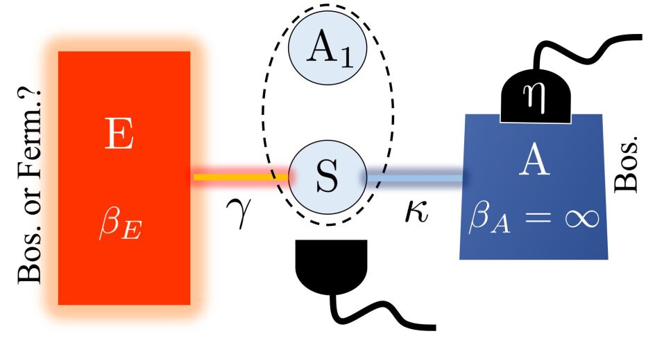
Figure 1: Schematic representation of the QBT setup: the statistical nature (Bosonic or Fermionic) of the thermal bath $E$ is determined studying the modifications it induces on a quantum probe $S$ (a qubit) that has been put in thermal contact with it, while interacting with a zero-temperature Bosonic auxiliary bath $A$ that is continuously monitored in time via photo-detection or homodyne measurements. In the picture $\gamma$, $\kappa$ are the two decay rates of the unconditional evolution of $S$ for the interaction with $E$ and $A$, respectively, while $\eta$ is the quantum efficiency of the continuous detection on $A$. We also allow for the possibility of initially entangling $S$ with an external qubit memory $A_{1}$ dynamically decoupled from all the other components of the setup, and performing joint detection on the system $SA_{1}$.

The QBT model we study is schematically sketched in Fig 1. A part from $E$ (the thermal environment whose statistical nature we wish to determine) and $S$ (the quantum probe that is put in interaction with $E$), it includes two extra elements which were not present in the original QBT scheme discussed in Refs. Farina et al. (2019); Gianani et al. (2020): namely an auxiliary bath $A$ whose statistical and thermodynamics properties are assumed to be known and which is also attached to $S$, and an external quantum memory $A_{1}$ that is dynamically decoupled from all the other components of the setup. As in Ref. Farina et al. (2019); Gianani et al. (2020), our goal is to decide whether $E$ is a Bosonic bath with assigned inverse temperature $\beta_{B}$ (hypothesis ${B}$), or Fermionic with assigned temperature $\beta_{F}$ (hypothesis ${F}$), the initial priors of these two alternatives being flat. To solve such a task we are allowed to prepare $S$ (that for simplicity we assume to be a qubit) in any desired input configuration, possibly correlated with the memory $A_{1}$, let it evolve for some time $t$ and perform measurements during and/or at the end of the process. The possibility of employing correlated states of $S$ and $A_{1}$ was not exploited in Ref. Farina et al. (2019); Gianani et al. (2020) and as we shall see allows for some useful technical improvements. The main difference of our proposal however is the presence of the auxiliary bath $A$ which we schematize as a zero-temperature multi-mode e.m. (hence Bosonic) field. Its role is to induce positive interference effects on the $S$-$E$ coupling and to permit continuous monitoring in time of the system evolution via photo-detection or or homodyne measurements (a configuration which may physically correspond to the case where we put $S$ into dispersive QED cavity).

II.1 Dynamical evolution

In this section we derive the dynamical equations that determine the temporal evolution of the system.

Let us start first by considering the case where the probe interacts with $E$ and $A$ in the absence of continuous monitoring of the latter. Following Ref. Farina et al. (2019) we model the $S$-$E$ and $S$-$A$ couplings via a Gorini-Kossakowski-Sudarshan-Lindblad (GKSL) master equation  Gorini et al. (1976); Lindblad (1976), a situation realized under the weak-coupling and Markovian hypotheses Breuer et al. (2002). Accordingly, defining $\mathcal{D}_{[\hat{\theta}]}$ to be the dissipative superoperator

$$\mathcal{D}_{[\hat{\theta}]}\bullet:=\hat{\theta}\bullet\hat{\theta}^{\dagger}-\frac{1}{2}\left\{\hat{\theta}^{\dagger}\hat{\theta},\bullet\right\}\leavevmode\nobreak\ ,$$ (1)

we write the dynamical evolution of the joint density matrix ${\hat{\varrho}}_{q}(t)$ of the probe $S$ and the memory $A_{1}$ as

$$\frac{d{\hat{\varrho}}_{q}(t)}{dt}=\mathcal{L}_{q}{\hat{\varrho}}_{q}(t)+\kappa\mathcal{D}_{[\hat{c}]}{\hat{\varrho}}_{q}(t)\leavevmode\nobreak\ ,$$ (2)

where the index $q\in\{B,F\}$ is used to specify which hypothesis has been selected for the statistical nature of $E$. In this equation $\mathcal{L}_{q}$ is the GKSL dynamical generator which accounts for the free evolution and for the $S-E$ coupling, i.e.

$$\mathcal{L}_{q}\bullet:=-i[\hat{H}_{S},\bullet]+\gamma[1+s_{q}N_{q}(\beta_{q})]\mathcal{D}_{[\hat{\sigma}_{-}]}\bullet+\gamma N_{q}(\beta_{q})\mathcal{D}_{[\hat{\sigma}_{+}]}\bullet,$$ (3)

where $\hat{H}_{S}:=\omega_{0}\hat{\sigma}_{+}\hat{\sigma}_{-}$ is the Hamiltonian of the probe, $\gamma$ is a positive coupling constant that fixes the timescale of the $S$-$E$ interaction, and where, having set $s_{q=B}=1$ and $s_{q=F}=-1$, $N_{q}(\beta):=1/({e^{\beta\omega_{0}}-s_{q}})$ is the Bose-Einstein/Fermi-Dirac factor: notice that $\hbar$ has been set equal to $1$ and that no free Hamiltonian has been assumed for $A_{1}$ which effectively participates to the process only through initial correlations with $S$ that have been possibly established at the beginning of the dynamical evolution. The second term in the l.h.s of Eq. (2) represents instead the $S$-$A$ coupling with the operator $\hat{c}$ selected depending on the type of interaction one has engineered, and with $\kappa\geq 0$ being a parameter that gauges its intensity – in particular setting $\kappa=0$ we recover the model discussed in Refs. Farina et al. (2019); Gianani et al. (2020). In the following we will consider the two cases $\hat{c}=\hat{\sigma}_{-}$ and $\hat{c}=\hat{\sigma}_{x}/2$: the first one corresponds to the a purely dissipative model where $S$ looses energy in favour to $A$ via spontaneous emission, while the second choice can be obtained via dispersive coupling that can be engineered e.g. in circuit-QED systems Hacohen-Gourgy et al. (2016); Chantasri et al. (2018); Hacohen-Gourgy and Martin (2020).

As already mentioned, Eq. (2) does not include effects associated with a continuous monitoring of $A$. To account for the latter we resort to the stochastic master equations (SME) approach of Refs. Wiseman and Milburn (2009); Jacobs and Steck (2006). In particular we will focus on two kind of measurements, photodetection and homodyne detection with a fixed monitoring efficiency $\eta$. In the case of photodetection, under hypothesis $q$, the corresponding SME for the conditional state of $SA_{1}$ reads

$$d{\hat{\varrho}}^{c}_{q}(t) =\mathcal{L}_{q}{\hat{\varrho}}_{q}^{c}(t)\,dt+(1-\eta)\kappa\mathcal{D}_{[\hat{c}]}{\hat{\varrho}}_{q}^{c}(t)$$ (4)

$$\,-\frac{\eta\kappa}{2}\mathcal{H}_{[\hat{c}^{\dagger}\hat{c}]}{\hat{\varrho}}^{c}_{q}(t)\,dt+\left(\frac{\hat{c}{\hat{\varrho}}^{c}_{q}(t)\hat{c}^{\dagger}}{\operatorname{Tr}[\hat{c}{\hat{\varrho}}^{c}_{q}(t)\hat{c}^{\dagger}]}-{\hat{\varrho}}^{c}_{q}(t)\right)dN_{t}\,,$$

where $dN_{t}\in\{0,1\}$, corresponds physically to the number of photons detected at each time $t$ and mathematically to a Poisson increment defined by its probability of taking value equal to one, $p(dN_{t}=1)=\eta\kappa\operatorname{Tr}[{\hat{\varrho}}^{c}_{q}(t)\hat{c}^{\dagger}\hat{c}]\,dt$, and where we have introduced the superoperator

$$\mathcal{H}_{[\hat{\theta}]}\bullet:=\hat{\theta}\bullet+\bullet\hat{\theta}^{\dagger}-\operatorname{Tr}[(\hat{\theta}^{\dagger}+\hat{\theta})\bullet]\bullet\,.$$ (5)

Similarly, in the case of homodyne detection one obtains the SME

$$d{\hat{\varrho}}^{c}_{q}(t)=\mathcal{L}_{q}{\hat{\varrho}}_{q}^{c}(t)\,dt+\kappa\mathcal{D}_{[\hat{c}]}{\hat{\varrho}}^{c}_{q}(t)\,dt+\sqrt{\eta\kappa}\mathcal{H}_{[\hat{c}]}{\hat{\varrho}}^{c}_{q}(t)\,dW_{t}\,,$$ (6)

where the state is conditioned on the continuous output photocurrent

$$dy_{t}:=\sqrt{\eta\kappa}\operatorname{Tr}[{\hat{\varrho}}^{c}_{q}(t)(\hat{c}+\hat{c}^{\dagger})]\,dt+dW_{t}\,,$$ (7)

and where $dW_{t}$, denoting the difference between the measurement output $dy_{t}$ and the expected results, mathematically corresponds to a Wiener increment s.t. the relation $dW_{t}^{2}=dt$ holds deterministically. We remark that by choosing as jump operators the ones defined before, i.e. either $\hat{c}=\hat{\sigma}_{-}$ or $\hat{c}=\hat{\sigma}_{x}/2$, one obtains photocurrents (7) with the same form, yielding information on the average value of the operator $\hat{\sigma}_{x}$. However the two operators will induce different dynamics, described by the corresponding SMEs (6).

For both photodetection and homodyne detection strategies, the associated SME (4) and (6) can be numerically integrated following the method based on Kraus operators suggested in Rouchon (2014); Rouchon and Ralph (2015) that we review in brief in Appendix A. This results in a collection of quantum trajectories for the conditional density matrix $\hat{\varrho}_{q}^{c}(t)$ each identified by a string of records

$$D_{t}:=(x_{t_{0}+dt},x_{t_{0}+2dt},\dots,x_{t-dt},x_{t})\leavevmode\nobreak\ ,$$ (8)

where we have assumed to perform measurements every infinitesimal time-interval $dt$ starting from the initial time $t_{0}$ (which we set to zero hereafter) and stopping at time $t$, and where for the photodetection and homodyne detection scenario the $x_{t}$’s correspond either to recorded values of $dN_{t}$ or $dy_{t}$ respectively. It is worth pointing out that, in principle, by averaging over all such solutions, i.e. by averaging $\hat{\varrho}_{q}^{c}(t)$ over all the obtained measurement results (8) up to a time $t$ or equivalently by fixing the monitoring efficiency $\eta=0$, one obtains an unconditional state solution that coincides with the standard master equation (2) of the problem, i.e.

$$\mathbbm{E}[\hat{\varrho}_{q}^{c}(t)]=\left.\hat{\varrho}_{q}^{c}(t)\right|_{\eta=0}=\hat{\varrho}_{q}(t)\;.$$ (9)

II.2 Quantum hypothesis testing in continuously monitored quantum systems

In this section we review the methods that allow us to characterize how efficiently one can solve the QBT problem we are facing.

To begin with, consider first the simple case where the data from the continuous monitoring in time are neglected, e.g. by averaging them away or setting $\eta=0$, a regime in which thanks to (9) the evolution of the system is provided by the master equation (2). Having hence selected an input state ${\hat{\varrho}}(0)$ for the $SA_{1}$ system and a total evolution time $t$, what we have to do is to determine whether at the end of the process the state of $SA_{1}$ is better described by the density matrix ${\hat{\varrho}}_{B}(t)$ or by the density matrix ${\hat{\varrho}}_{F}(t)$ obtained by solving Eq. (2) under the two alternative QBT hypotheses. This problem can be easily framed as a special instance of quantum hypothesis testing Helstrom (1969): accordingly we can bound the error probability associated with the selected strategy through the Helstrom inequality

$$p_{err}(t;{\hat{\varrho}}(0)) \geq {\rm HEP}(t;{\hat{\varrho}}(0))\;,$$ (10)

$${\rm HEP}(t;{\hat{\varrho}}(0)) := \frac{1}{2}\left(1-\frac{\|{\hat{\varrho}}_{B}(t)-{\hat{\varrho}}_{F}(t)\|_{1}}{2}\right),$$ (11)

where $\lVert\bullet\lVert_{1}$ denotes the trace norm, and where we used the fact that the prior probability associated with the events $B$ and $F$ is flat. The threshold value ${\rm HEP}(t;{\hat{\varrho}}(0))$, conventionally called the Helstrom error probabilitiy, can always be attained via a projective measurement on $SA_{1}$ that at time $t$ distinguishes the positive and negative eigenstates of the operator ${\hat{\varrho}}_{B}(t)-{\hat{\varrho}}_{F}(t)$. Accordingly in Refs. Farina et al. (2019); Gianani et al. (2020) ${\rm HEP}(t;{\hat{\varrho}}(0))$ was used as a bona-fide quality factor for the QBT efficiency one can achieve with the selected choice of $t$ and ${\hat{\varrho}}(0)$. Notice however that in such works ${\hat{\varrho}}_{B}(t)$ and ${\hat{\varrho}}_{F}(t)$ referred to the local states of $S$ (i.e. the presence of the external quantum memory $A_{1}$ was not allowed) and, most importantly, the auxiliary bath $A$ was not included in the picture (a condition which in our modelization corresponds to set $\kappa=0$ in Eq. (2)). As we shall see in the next section, even without resorting to continuous monitoring in time, lifting these two constraints already allows one for some non trivial improvements on the minimum error probability value.

Let’s now address the QBT problem and continuous monitoring assumptions. As described in Kiilerich and Mølmer (2018), in this case the hypothesis testing can follow two different approaches: in order discriminate between the two hypotheses, one may exploit the continuous experimental data $D_{t}$ only, or one can also implement a final direct measurement on $S$ and $A_{1}$ on the corresponding conditional states. We now start to asses the first scenario. In this case one can resort to a Bayesian analysis, by first observing that each trajectory $D_{t}$ is characterized by a probability $P(D_{t}|q)$, when conditioning on the initial assumption that the bath is defined by a statistics associated with the QBT hypothesis $q$. Hence, introducing a likelihood $L(D_{t}|q)=P(D_{t}|q)/p_{0}(D_{t})$ with $p_{0}(D_{t})$ denoting a positive function of $D_{t}$ only Kiilerich and Mølmer (2018), and by resorting to Bayes theorem, it is possible to compute the a-posteriori probability as

$$P(q|D_{t})=\frac{P(D_{t}|q)}{\sum_{q^{\prime}}P(D_{t}|q^{\prime})}=\frac{L(D_{t}|q)}{\sum_{q^{\prime}}L(D_{t}|q^{\prime})}\,,$$ (12)

which we present here exploiting the fact that the flat prior distribution on $q$ is flat (the specific definition of $L(D_{t}|q)$ and the method to efficiently compute it is discussed in details in Appendix A). Observe next that as (12) is normalized for each values of the QBT hypothesis index $q$ we have two possibilities, namely $P(q|D_{t})\geq 1/2$, in such a case the bath is most likely to be of $q$ nature, and $P(q|D_{t})<1/2$ in which the opposite hypothesis is more plausible. However, the inherent stochasticity of the measurement outcomes can result in $P(B|D_{t})\geq 1/2$ ($P(F|D_{t})\geq 1/2$) even if the statistics of the bath was Fermionic (resp. Bosonic), i.e. there are measurement records that may lead to a wrong inference process. The goal is thus to quantify the probability of occurrence of such wrong tagging events. In the spirit of a thought experiment, we consider a sample of $N_{traj}$ trajectories $D_{t}$, supposing that half of them are generated by indirectly probing a Bosonic environment ($D^{B}_{t}$), while the rest are Fermionic ($D^{F}_{t}$). A wrong tagging event is triggered every time we have a trajectory $D^{q}_{t}$ such that $P(q|D^{q}_{t})<1/2$. Counting the number $N_{wrong}$ of such trajectories leads to a first way to quantify the error probability as the following ratio

$$p_{err}^{(cont)}(t;{\hat{\varrho}}(0)):=\frac{N_{wrong}}{N_{traj}}\leavevmode\nobreak\ ,$$ (13)

where the notation stresses the implicit dependence upon the specific choice of the input state ${\hat{\varrho}}(0)$ of $SA_{1}$ and on the total evolution time $t$.

As mentioned before, a discrimination capability higher than (13) can in principle be achieved by improving our continuous monitoring scheme with the addition of a Helstrom projective measurement on $S$ and $A_{1}$ at the final time $t$. In this case the ultimate bound for the error probability is given by the Helstrom bound (11), for the two quantum states $\hat{\varrho}_{B,F}^{c}(t)$, solutions of the SMEs (4) or (6) for the dataset $D_{t}$, and obtained numerically via Eq. (34), with prior probabilities $P(q|D_{t})$. In formula we obtain the following non linear functional of the detector records

$${\rm HEP}^{c}(t;\hat{\varrho}(0)):=\frac{1-\left\lVert P(F|D_{t})\hat{\varrho}_{F}^{c}(t)-P(B|D_{t})\hat{\varrho}_{b}^{c}(t)\right\lVert_{1}}{2}\leavevmode\nobreak\ .$$ (14)

We remark that, apart influencing the dynamics of the density matrices $\hat{\varrho}_{b}^{c}(t)$ and $\hat{\varrho}_{F}^{c}(t)$, the knowledge coming from continuous monitoring updates the two priors probabilities Kiilerich and Mølmer (2018), and in general indentifies the optimal Helstrom projective measurement. An average over all the $N_{traj}$ trajectories of our sample returns the following figure of merit

$$p_{err}^{(cont+proj)}(t;\hat{\varrho}(0)):=\mathbbm{E}\left[{\rm HEP}^{c}(t;\hat{\varrho}(0))\right]\leavevmode\nobreak\ ,$$ (15)

that thus takes into account the average information gained from both the continuous monitoring and from a final Helstrom projective measurement for each trajectory.

III Analysis/Results

In this section we will present our main results. We will start by discussing the standard QBT scenario presented in Farina et al. (2019), but allowing the system to be entangled with a qubit ancilla. We will then study how the presence of the auxiliary bath $A$ can be useful in solving the quantum hypothesis testing problem even in the absence of the continuous monitoring (an effected which we can dub noise-assisted scenario). Finally we address the continuous-monitoring scenario showing how the indirect information obtainable from $A$ could help in the discrimination strategy.

III.1 Advantage from initial entanglement

As already discussed in the previous sections in the original QBT schemes of Refs. Farina et al. (2019); Gianani et al. (2020) the probing system $S$ was not correlated with external memory elements. We argue here that adding $A_{1}$ into the picture already introduces some major advantages, even in the absence of the extra auxiliary bath $A$ and of its continuous monitoring in time. To see this explicit let us introduce ${\cal E}_{q,t}$ the Linear, Completely Positive, Trace Preserving (LCPT) channel Watrous (2018); Holevo (2011) that allows one to express the solution of Eq. (2) as $\hat{\varrho}_{q}(t)={\cal E}_{q,t}\hat{\varrho}(0)$. Observe hence that, for fixed $t$, the minimal value that the HEP function of Eq. (10) can attain can be expressed as

$${\rm HEP}(t;{\hat{\varrho}}(0))\geq{\rm HEP}_{\diamond}(t):=\frac{1}{2}\left(1-\frac{\|{\cal E}_{B,t}-{\cal E}_{F,t}\|_{\diamond}}{2}\right),$$ (16)

with

$$\|{\cal E}_{B,t}-{\cal E}_{F,t}\|_{\diamond}:=\max_{\hat{\varrho}(0)\in\mathfrak{S}_{SA_{1}}}\|{\cal E}_{B,t}\hat{\varrho}(0)-{\cal E}_{F,t}\hat{\varrho}(0)\|_{1}\;,$$ (17)

being the the diamond norm distance Kitaev (1997); Kitaev et al. (2002) obtained by maximizing over the set of $\mathfrak{S}_{SA_{1}}$ of the input joint density matrices of $S$ and $A_{1}$. The term ${\rm HEP}_{\diamond}(t)$ of (16) should be compared with the quantity

$${\rm HEP}_{1}(t):=\frac{1}{2}\left(1-\frac{\|{\cal E}_{B,t}-{\cal E}_{F,t}\|_{1}}{2}\right)\;,$$ (18)

with

$$\|{\cal E}_{B,t}-{\cal E}_{F,t}\|_{1}:=\max_{\hat{\varrho}(0)\in\mathfrak{S}_{S}}\|{\cal E}_{B,t}\hat{\varrho}(0)-{\cal E}_{F,t}\hat{\varrho}(0)\|_{1},$$ (19)

which represents instead the optimal QBT error probability one can get by restricting the analysis to only local density matrices of $S$ as assumed in Refs. Farina et al. (2019); Gianani et al. (2020). The fact that using $A_{1}$ can provide better QBT performances then follows simply by the natural ordering between the diamond norm distance and the corresponding trace norm distance Watrous (2018), which implies $\|{\cal E}_{B,t}-{\cal E}_{F,t}\|_{\diamond}\geq\|{\cal E}_{B,t}-{\cal E}_{F,t}\|_{1}$, and hence

$${\rm HEP}_{1}(t)\geq{\rm HEP}_{\diamond}(t)\;.$$ (20)

A quantitive evaluation of the advantages implied by Eq. (20) can be attained by focusing on the scenario where $A$ is disconnected (i.e. $\kappa=0$) and the temperature of $E$ in two QBT hypothesis is the same, i.e. $\beta_{B}=\beta_{F}=\beta$, and sufficiently large, i.e. $\beta\rightarrow 0$. Under these conditions, the rescaled rate constants corresponding to the Bosonic hypothesis, i.e. $q=B$, diverge while those for the Fermionic hypothesis, i.e. $q=F$, remain finite. As a consequence the Bosonic channel ${\cal E}_{B,t}$ will imply immediate thermalization of $S$, in the sense that it leads to thermalization of the probe system on time scales $\tau$ where the Fermionic channel ${\cal E}_{F,t}$ has not significantly affected the dynamics yet, i.e. formally

$${\cal E}_{B,\tau}\bullet\simeq\hat{\varrho}_{\beta}\otimes\mbox{Tr}_{S}[\bullet]\;,\qquad{\cal E}_{F,\tau}\bullet\simeq{\cal I}\bullet\;,$$ (21)

with

$$\hat{\varrho}_{\beta}:=\exp(-\beta\hat{H}_{S})/{\rm tr}[\exp(-\beta\hat{H}_{S})]\;,$$ (22)

the Gibbs thermal state of the probe, $\mbox{Tr}_{S}[\bullet]$ represents the partial trace with respect to $S$, and ${\cal I}$ is the identity superoperator. Choosing hence the initial state $\hat{\varrho}(0)$ of $S$ and $A_{1}$ to be the maximally entangled state

$$\ket{\Phi^{+}}:=(\ket{11}_{SA_{1}}+\ket{00}_{SA_{1}})/\sqrt{2}\;,$$ (23)

from (11) we get

$$\|{\cal E}_{B,\tau}\hat{\varrho}(0)-{\cal E}_{F,\tau}\hat{\varrho}(0)\|_{1} \simeq \left\|{\hat{\varrho}}(0)-\hat{\varrho}_{\beta}\otimes\frac{\mathbb{1}}{2}\right\|_{1}$$

$$\simeq \left\|\ket{\Phi^{+}}\bra{\Phi^{+}}-\frac{\mathbb{1}}{2}\otimes\frac{\mathbb{1}}{2}\right\|_{1}=\frac{3}{2}\;,$$

where in the second line we invoke the $\beta\rightarrow 0$ limit to approximate $\hat{\varrho}_{\beta}\simeq\mathbb{1}/{2}$. Replacing this into Eq. (11) gives finally

$${\rm HEP}(\tau;\ket{\Phi^{+}})\simeq 1/8\;,$$ (25)

which should be compared with the values one would get by discarding $A_{1}$ from the problem, i.e. forcing $\hat{\varrho}(0)$ to be a local density matrix of just $S$. Under this circumstance, Eq. (III.1) gets replaced by

$$\|{\cal E}_{B,\tau}\hat{\varrho}(0)-{\cal E}_{F,\tau}\hat{\varrho}(0)\|_{1}\simeq\left\|{\hat{\varrho}}(0)-\hat{\varrho}_{\beta}\right\|_{1}\simeq\|{\hat{\varrho}}(0)-{\mathbb{1}}/{2}\|_{1}\leq 1\;,$$ (26)

with the last inequality being reachable by taking $\hat{\varrho}(0)$ pure, e.g. the vector $|1\rangle$. Accordingly we can write

$${\rm HEP}_{1}(\tau)={\rm HEP}(\tau;|1\rangle)\simeq{1}/{4}\;,$$ (27)

which is twice the minimum value (25) attained by using as input for $S$ and $A_{1}$ the maximally entangled state (23).

III.2 Noise-assisted QBT

In this section we show that the presence of the additional environment $A$ can enhance the QBT procedure even when $A$ is not continuously monitored, i.e. for $\kappa>0$ but $\eta=0$ so that the equation of motion of the system is governed by Eq. (2). Since in this case $A$ introduces only extra dissipative effects in the dynamics of $S$ we dub such enahacement noise-assisted QBT. As we shall see the origin of this phenomenon can be traced back to the fact that adding $A$ into the picture (i.e. passing from $\kappa=0$ to $\kappa\neq 0$ in Eq. (2)) modifies the dynamical process which is responsible for the encoding of the statistical nature of $E$ on the $SA_{1}$ system. While in a generic metrology setting there is no guaranty that such interference will have positive effects, the theory does not prevent that for some special task this could happen: the QBT problem we present here is one (indeed to our knowledge probably the first) of the such special examples.

To enlighten the possibility of exploiting the mere presence of $A$ to boost the QBT performances it is useful to consider the scenario where the two QBT hypothesis are characterized by the same temperature (i.e. $\beta_{B}=\beta_{F}=\beta$): under this condition for $t$ sufficiently large, the contact with $E$ alone ($\kappa=0$) will lead $S$ to the Gibbs state (22), regardless to the nature of the bath hence making the QBT discrimination impossible Farina et al. (2019). Yet there is a chance that by taking $\kappa\neq 0$, the simultaneous interactions of $S$ with $E$ and $A$ will interfere leading to departures from such dead-end behaviour paving the way for improvements of the discrimination efficiency even for large $t$ (it is also clear however that one also expect that in order to be beneficial, such deviations should not be too strong so that the $S$-$E$ coupling gets completely dominated by the $S$-$A$ interaction). To see this explicitly let us study the values that the HEP figure of merit ${\rm HEP}(t;{\hat{\varrho}}(0))$ of Eq. (11) attains in the asymptotic regime of $t\rightarrow\infty$ as a function of $\kappa$, considering the scenario where the $S$-$A$ interaction is mediated by the operator $\hat{c}=\hat{\sigma}_{-}$ (dissipative coupling). In this case, irrespectively from the choice of the initial state ${\hat{\varrho}}(0)$ of $S$ and $A_{1}$, we obtain the following steady state HEP value

$${\rm HEP}(t\rightarrow\infty)=\frac{1}{2}-\frac{1}{2\omega_{0}\kappa}\Big{|}\dot{Q}^{(E_{B}\Rightarrow A)}-\dot{Q}^{(E_{F}\Rightarrow A)}\Big{|}\leavevmode\nobreak\ ,$$ (28)

where $\dot{Q}^{(E_{q}\Rightarrow A)}$ denotes the heat flows from $E$ to $A$ associated with the QBT hypotheses $q=B,F$, i.e. the quantities

$${\dot{Q}^{(E_{B}\Rightarrow A)}=}\omega_{0}\kappa\;\frac{N_{B}(\beta_{B})}{1+2N_{B}(\beta_{B})+\kappa/\gamma}\leavevmode\nobreak\ ,$$ (29)

$${\dot{Q}^{(E_{F}\Rightarrow A)}=}\omega_{0}\kappa\;\frac{N_{B}(\beta_{F})}{1+2N_{B}(\beta_{F})+[1+2N_{B}(\beta_{F})]\kappa/\gamma}\leavevmode\nobreak\ ,$$

which we report here for arbitrary choices of $\beta_{B}$ and $\beta_{F}$. The result (28) holds also for the case $\hat{c}=\hat{\sigma}_{x}/2$, up to a numerical factor and different expressions for the heat flows (see Appendix B for the derivation of all the results). As anticipated we notice that for $\beta_{B}=\beta_{F}=\beta$ and $\kappa=0$, one gets ${\rm HEP}(t\rightarrow\infty)=1/2$ signalling the impossibility of solving the QBT problem Farina et al. (2019). We observe also that for $\kappa\gg\gamma$ one has ${\rm HEP}(t\rightarrow\infty)=1/2$ signalling that the large disturbance originated by $A$ nullifies the sensitivity to the statistics of the bath $E$. Most interestingly however when $\kappa$ is finite we get a clear advantage with respect to the $\kappa=0$ case, see Fig. 2. The physical interpretation of such noise-assisted QBT improvement is that since $A$ is a zero-temperature bath there is finite average heat flowing from the hot bath $E$ with ${q}=B,F$ that can be monitored by the probe: the non-zero discrimination capability hence follows due to the fact that a Fermionic $E$ implies a slower heat transfer from $E$ to $S$ than a Bosonic $E$. Figure 2 makes also evident that there exists in particular an optimal coupling constant $\kappa$ minimizing (28), that for $\hat{c}=\hat{\sigma}_{-}$ can be analytically evaluated as

$$\kappa_{best}/\gamma=\sqrt{2N_{B}(\beta)+1}\leavevmode\nobreak\ ,$$ (30)

(when the $S$-$A$ is mediated by the operator $\hat{c}=\hat{\sigma}_{x}/2$ the optimal value is twice as above – see Appendix B).

A similar analysis can also be conducted for the case of asymmetric temperatures ($\beta_{B}\neq\beta_{F}$): here however the model naturally allows also for discrimination at steady state also in the case $\kappa=0$, as already studied in Gianani et al. (2020). Accordingly, while in some regimes one can still get improvements by working with $\kappa\neq 0$ the study become slightly more involved and possibly less interesting. Instead we would like to report the fact that in this unequal temperature scenario there can be critical $\kappa$ values

$$\kappa_{c}/\gamma=\frac{N_{B}(\beta_{F})-N_{B}(\beta_{B})}{N_{B}(\beta_{B})[1+2N_{B}(\beta_{F})]-N_{B}(\beta_{F})}$$ (31)

where QBT discrimination is made impossible (i.e. $H(t\rightarrow\infty)=1/2$) by the presence of $A$, see the dashed line in Fig. 2. For the $\hat{c}=\hat{\sigma}_{-}$ coupling this is actually happening if and only if either we have

$$\frac{1}{2}<N_{B}(\beta_{B})<N_{B}(\beta_{F})\;,$$ (32)

or

$$N_{B}(\beta_{B})<N_{B}(\beta_{F})<\frac{N_{B}(\beta_{B})}{1-2N_{B}(\beta_{B})}\leavevmode\nobreak\ .$$ (33)

This last property marks a difference with the noise assisted QBT with $\hat{c}=\hat{\sigma}_{x}/2$ where a non zero discrimination capability at steady state for $\kappa$ finite may occur but the critical points appear only for $N_{B}(\beta_{B})\geq N_{B}(\beta_{F})$ (see Appendix B). In summary, the additive noise implied by an engineered additional environment on the one hand can open the discrimination window for two baths at the same temperature, on the other hand can prevent discrimination of two baths at different temperatures when choosing “unlucky” values of the loss coefficient.

\begin{overpic}[width=346.89731pt]{fig2.pdf} \put(90.0,65.0){} \end{overpic}

Figure 2: Plots of the noise-assisted Helstrom bound ${\rm HEP}(t\rightarrow\infty)$ reported in Eq. (28), as function of $\kappa/\gamma$. Solid blue line: isothermal QBT scenario $\beta_{B}=\beta_{F}=\beta$ with $N_{B}(\beta)=2$. Dashed red line: example of an asymmetric temperature QBT scenario ($N_{B}(\beta_{B})=1$, $N_{B}(\beta_{F})=2$). Here we notice that ${\rm HEP}(t\rightarrow\infty)$ is smaller than $1/2$ for $\kappa=0$, reaching instead the zero discrimination threshold at an intermediate critical value determined by Eq. (31).

III.3 Monitoring-enhanced QBT

We now discuss the performance in the QBT protocol when the additional environment can be continuously monitored, by considering the two scenarios corresponding to either flourescence or dispersive monitoring corresponding respectively to the jump operators $\hat{c}=\hat{\sigma}_{-}$ or $\hat{c}=\hat{\sigma}_{x}/2$. We remind that under these circumstances the system dynamics is described by the SME (4) or (6) depending on the type of measurements we have selected, and that the attainable mean error probability can be evaluated either in terms of the functional $p_{err}^{(cont)}(t;{\hat{\varrho}}(0))$ of Eq. (13), or in terms of its improved version $p_{err}^{(cont+proj)}(t;\hat{\varrho}(0))$ of Eq. (15), depending on whether or not we allow for a final Helstrom measurement on $S$ and $A_{1}$. In an effort to simplify the study in what follows we shall fix as input state for $SA_{1}$ the maximally entangled state (23) – the only exception being for the data reported in panel (a) of Fig. 3 where we assume $S_{1}$ to be uncorrelated with $A_{1}$. While in principle for given $t$ this is possibly not the optimal choice in terms of the diamond norm requirement, the choice is an educated guess as its evolved counterpart is nothing but the Choi-Jamiolkowski state Watrous (2018); Holevo (2011) of the associated dynamical map that is known to provide a faithful representation of the latter.

\begin{overpic}[width=346.89731pt]{fig3a.pdf} \put(50.0,55.0){\color[rgb]{0,0,0} input $\ket{0}$} \put(90.0,65.0){(a)} \end{overpic}

\begin{overpic}[width=346.89731pt]{fig3b.pdf} \put(50.0,55.0){\color[rgb]{0,0,0} input $\ket{\Phi^{+}}$} \put(90.0,65.0){(b)} \end{overpic}

Figure 3: Plot of $p_{err}^{(cont+proj)}$, Eq. (15), for the different values of the efficiency $\eta$ reported in the legend. In panel (a) we choose the input state of $S$ to be the ground state of its local Hamiltonian, while in panel (b) we consider as input of $S$ and $A_{1}$ the maximally entangled state $\ket{\Phi^{+}}$. All data in the figure are obtained in the isothermal QBT scenario $\beta_{B}=\beta_{F}=\beta$, for $\beta\omega_{0}=1/5.5$; $\kappa/\gamma=1$ and by considering the jump operator $\hat{c}=\hat{\sigma}_{-}$.

III.3.1 Purely dissipative $S$-$A$ coupling regime

Here we focus on the case where $S$ and $A$ interact through the jump operator $\hat{c}=\hat{\sigma}_{-}$.

The usefulness of exploiting the knowledge deriving from the continuous monitoring of $A$ are well enlightened in Fig. 3 where for brevity we only focus on homodyne-detection: in this figure the quantity $p_{err}^{(cont+proj)}(t)$ is plotted as function of $t$, for different choices of the quantum efficiency $\eta$. As intuitively expected increasing $\eta$ leads to better discrimination performance: in particular the worst case scenario is obtained for $\eta=0$ (blue curves in the plot, corresponding to the noise-assisted strategy where we do not monitor $A$), while the best case is associated with $\eta=1$ (black dash-dotted curve, corresponding to perfect detection efficiency).

We then fix the monitoring efficiency to its maximum value $\eta=1$ and turn our attention to the coupling $\kappa$ that gauges the $S$-$A$ coupling, which in this framework can be also interpreted as a measurement strength. The results are depicted in the panels (a), (b), (d) and (e) of Fig. 4 where in the top (bottom) panels we show the behaviour of $p_{err}^{(cont)}(t)$ ($p_{err}^{(cont+proj)}(t)$) for different values of $\kappa$. The first thing one may notice is that for low values of $\kappa$ photo-detection is less efficient than homodyne in reducing $p_{err}^{(cont)}(t)$, while for large values of $\kappa$ it becomes the preferable choice – see panels (a) and (b). Regarding $p_{err}^{(cont+proj)}(t)$ independently on the type of detection on $A$, we can make two relevant observations: (i) at short time scales the monitoring of $A$ does not lead to a better discrimination as indeed the optimal value still corresponds to the case $\kappa=0$ (blue curves in the figure); (ii) on the other hand, at long time scales the cumulative information acquired by continuous monitoring definitely improves discrimination for increasing values of $\kappa$. In particular we have numerical evidence that both $p_{err}^{(cont)}(t)$ and $p_{err}^{(cont+proj)}(t)$ go to zero in the long time limit, and thus that in general the minimum error probability obtainable for $\kappa=0$ can be overcome by considering either $\kappa$ and/or time large enough – see Fig. 5.

\begin{overpic}[width=130.08731pt]{fig4a.pdf} \put(20.0,45.0){$\hat{c}=\hat{\sigma}_{-}$} \put(90.0,65.0){(a)} \end{overpic}

\begin{overpic}[width=130.08731pt]{fig4b.pdf} \put(20.0,45.0){$\hat{c}=\hat{\sigma}_{-}$} \put(90.0,65.0){(b)} \end{overpic}

\begin{overpic}[width=130.08731pt]{fig4c.pdf} \put(20.0,35.0){$\hat{c}=\hat{\sigma}_{x}/2$} \put(90.0,65.0){(c)} \end{overpic}

\begin{overpic}[width=130.08731pt]{fig4d.pdf} \put(20.0,45.0){$\hat{c}=\hat{\sigma}_{-}$} \put(90.0,65.0){(d)} \end{overpic}

\begin{overpic}[width=130.08731pt]{fig4e.pdf} \put(20.0,45.0){$\hat{c}=\hat{\sigma}_{-}$} \put(90.0,65.0){(e)} \end{overpic}

\begin{overpic}[width=130.08731pt]{fig4f.pdf} \put(20.0,45.0){$\hat{c}=\hat{\sigma}_{x}/2$} \put(90.0,65.0){(f)} \end{overpic}

Figure 4: Setting $\ket{\Phi^{+}}$ as initial state of the $SA_{1}$ system, we plot (a)-(c) $p_{err}^{(cont)}(t)$ and (d)-(f) $p_{err}^{(cont+proj)}(t)$ for different detection strategies: for $\hat{c}=\hat{\sigma}_{-}$ Photo-detection (a),(d) and Homodyne-detection (b),(e); and for $\hat{c}=\hat{\sigma}_{x}/2$ Homodyne-detection (c),(f). Different curves refer to different values of $\kappa$ as indicated in the legend with $\kappa=0$ referring to the case where $A$ is decoupled from the probe. All data in this figure are obtained in the isothermal QBT scenario $\beta_{B}=\beta_{F}=\beta$, setting $\beta\omega_{0}=1/5.5$ and $\eta=1$.

\begin{overpic}[width=424.94574pt]{fig5.pdf} \end{overpic}

Figure 5: Long time behaviour of $p_{err}^{(cont+proj)}(t)$ for different continuous monitoring strategies (see legend). All data are obtained in the isothermal QBT scenario $\beta_{B}=\beta_{F}=\beta$, setting $\beta\omega_{0}=1/5.5$, $\eta=1$, $\kappa/\gamma=1$ and considering $\ket{\Phi^{+}}$ as the initial state.

III.3.2 Dispersive $S$-$A$ coupling

Consider next the possibility of coupling dispersively the system to the environment $A$ represented by taking $\hat{c}=\hat{\sigma}_{x}$ as the jump operator of the model Hacohen-Gourgy et al. (2016). We start by observing that, as $\hat{c}^{\dagger}\hat{c}=\hat{\sigma}_{x}^{2}=\mathbbm{1}$, the probability for continuous photodetection is independent on the state, and thus it cannot contain any information on the bath $E$. For this reason for the photo-detection unravelling one would obtain $p_{err}^{(cont)}(t)=1/2$ at any time $t$. We thus show the result of $p_{err}^{(cont)}(t)$ for homodyne detection only, see panel (c) of Fig. 4, with the corresponding case of final projective measurement on $SA_{1}$ in panel (f). Also in this case, we find that at short time scales the coupling with $A$ and the monitoring is not helpful, as the best performances are observed for $\kappa=0$. On the other hand we find that $p_{err}^{(cont+proj)}(t)$ decreases towards zero at long time scales and that, as in the previous case, better results are obtained by increasing the coupling $\kappa$. We do not provide results for continuous photodetection with a final projective measurement as, while error probabilities below $1/2$ are observed, the performances are definitely worse respect to the other cases we have considered.

III.3.3 Strategies Comparision

We compare the three different strategies, continuous homodyne and photodetection with $\hat{c}=\hat{\sigma}_{-}$ and continuous homodyne with $\hat{c}=\hat{\sigma}_{x}/2$ in Fig. 5. We observe that in the long-time limit the two best strategies correspond to either performing continuous homodyne on an environment coupled dispersively via the jump operator $\hat{c}=\hat{\sigma}_{x}/2$ or continuous photodetection with jump operator $\hat{c}=\hat{\sigma}_{-}$. Moreover the first strategy is also the best one in the short-time limit (we remark that similar results are obtained numerically for different values of the parameters).

IV Conclusions and final remarks

In this work we have investigated the possibility of improving the performances of QBT task originally presented in Farina et al. (2019); Gianani et al. (2020) using extra auxiliary resources such as an extra memory element $A_{1}$ that could be initially entangled with the original probe $S$, and an extra environment $A$ that instead is allowed to interact with the $S$ while possibly being monitored continuously in time. In particular we notice that the QBT task can benefit even when $A$ is monitored very inefficiently ($\eta=0$), an effect that for instance is observed in the equal temperature case which for long interaction time would not allow for QBT discrimination in the original proposal Farina et al. (2019); Gianani et al. (2020). We finally compared the performances associated to different realizations of continuous monitoring of $A$ via photo-detection or homodyne, proving that a finite detection efficiency is naturally beneficial to the QBT task. Before concluding we would like to comment that the reported results, while derived in the specific QBT setting of  Farina et al. (2019); Gianani et al. (2020) can be generalized to improve the performances of arbitrary quantum hypothesis tasks, in particular in all those problems where an agent is asked to use an external probe to discriminate between alternative quantum trajectories associated with different dynamical quantum generators. We also would like to mention that experimental realizations for specific setup we have analyzed in the manuscript are feasible e.g. in the context of superconducting qubits Hacohen-Gourgy et al. (2016); Ficheux et al. (2018). In these models, assuming $S$ and $A_{1}$ to be superconducting transmon qubits, the initial entanglement configuration between them can be reached for example with the use of a common bus resonator Egger et al. (2019). Notice also that configurations where $S$ is capacitively coupled with two baths $E$ and $A$ (the latter being continuously monitored) are now experimentally under control, e.g. interpreting the $S$ as a quantum valve Ronzani et al. (2018). In particular in our case the engineered environment $A$ may consist in a cavity where this time only $S$ is embedded and the initial coupling with $A_{1}$ is now off-detuned, and the transmission of input microwave fields are used for quadrature and dispersive measurements Tan et al. (2015). Specifically either a fluorescence measurement Ficheux et al. (2018), corresponding to a jump operator $\hat{c}=\hat{\sigma}_{-}$, or a dispersive measurement Hacohen-Gourgy et al. (2016), corresponding for example to a jump operator $\hat{c}=\hat{\sigma}_{x}/2$, is performed by using a resonant field. The output for homodyne measurement is instead recorded via a Josephson parametric amplifier, or, in the case of heterodyne measurements, via a Josephson parametric converter Ficheux et al. (2018). The final Helstrom measurement on $SA_{1}$ can be generally achieved in these experiments by applying a strong, dispersively coupled probe field Murch et al. (2013); Tan et al. (2015); Kiilerich and Mølmer (2018).

V.G. acknowledges MIUR (Ministero dell’ istruzione, dell’ Universita’ e della Ricerca) via project PRIN 2017 “Taming complexity via QUantum Strategies a Hybrid Integrated Photonic approach” (QUSHIP) Id. 2017SRNBRK.

Appendix A Numerical integration of stochastic master equations

We here describe the method proposed in Rouchon (2014); Rouchon and Ralph (2015) in order to efficiently numerically integrate SMEs, as the ones reported in Eqs. (4) and (6). One proves that the quantum state solution of these SMEs can be written after each time step $dt$ as

$${\hat{\varrho}}^{c}_{q}(t+dt)=\frac{\sum_{k}\hat{M}^{(k)}_{x_{t}}\left[{\hat{\varrho}}^{c}_{q}(t)+\mathcal{L}_{q}{\hat{\varrho}}^{c}_{q}(t)dt\right]{\hat{M}_{x_{t}}^{(k)}}{}^{\dagger}}{\operatorname{Tr}(\sum_{k}\hat{M}^{(k)}_{x_{t}}\left[{\hat{\varrho}}^{c}_{q}(t)+\mathcal{L}_{q}{\hat{\varrho}}^{c}_{q}(t)dt\right]{\hat{M}_{x_{t}}^{(k)}}{}^{\dagger})}\,,$$ (34)

where we have introduced the Kraus operators $\hat{M}_{x_{t}}^{(k)}$ that describe the effect of the measurement, with outcome $x_{t}$, on the quantum state at each time $t$. The form of these operators depends on the kind of measurement that is performed. In the case of photodetection, the two Kraus operators corresponding to the two possible measurement outcomes $x_{t}=\{0,1\}$ are

$$\begin{cases}\hat{M}_{0}^{(1)}=\hat{\mathbbm{1}}-\frac{\kappa}{2}\hat{c}^{\dagger}\hat{c}\,dt\\ \hat{M}_{0}^{(2)}=\sqrt{(1-\eta)\kappa dt}\,\hat{c}\end{cases}\,,\qquad\qquad\hat{M}_{1}^{(1)}=\sqrt{\eta\kappa dt}\,\hat{c}\,,$$ (35)

that are applied according to the Poisson increment probabilities $p_{0}=1-\eta\kappa\operatorname{Tr}[{\hat{\varrho}}^{c}_{q}\hat{c}^{\dagger}\hat{c}]dt$ and $p_{1}=\eta\kappa\operatorname{Tr}[{\hat{\varrho}}^{c}_{q}\hat{c}^{\dagger}\hat{c}]dt$. As regards continuous homodyne detection, the continuous outcome corresponds to the photocurrent $x_{t}=dy_{t}$ and the corresponding Kraus operators have the form

$$\begin{cases}\hat{M}_{dy_{t}}^{(1)}=\hat{\mathbbm{1}}-\frac{\kappa}{2}\hat{c}^{\dagger}\hat{c}\,dt+\sqrt{\eta\kappa}\hat{c}\,dy_{t}\\ \hat{M}_{dy_{t}}^{(2)}=\sqrt{(1-\eta)\kappa dt}\,\hat{c}\end{cases}\,,$$ (36)

where the randomness of the process is originated by the Wiener increment entering in the formula for the photocurrent (7).

This numerical method also allows to evaluate straightforwardly the likelihood of each trajectory. In fact, at each time step, the likelihood of obtaining the measurement outcome $x_{t}$ can be evaluated by taking the trace of the operator at the numerator in Eq. (34), i.e.

$$l_{x_{t}}=\operatorname{Tr}[\tilde{\varrho}_{q}^{c}(t+dt)]\,,$$ (37)

where

$$\tilde{\varrho}_{q}^{c}(t+dt) =\sum_{k}\hat{M}^{(k)}_{x_{t}}\left[{\hat{\varrho}}^{c}_{q}(t)+\mathcal{L}_{q}{\hat{\varrho}}^{c}_{q}(t)dt\right]{\hat{M}_{x_{t}}^{(k)}}{}^{\dagger}\,.$$ (38)

As remarked in the main text, by assuming to start and stop the monitoring respectively at time $t_{0}$ and time $t$, each trajectory can be identified by the string of records $D_{t}$ of Eq. (8): the corresponding likelihood can thus be evaluated as

$$L(D_{t}|q)=\prod_{t^{\prime}=t_{0}}^{t}l_{x_{t^{\prime}}}=\prod_{t^{\prime}=t_{0}}^{t}\operatorname{Tr}[\tilde{\varrho}_{q}^{c}(t^{\prime}+dt)]\;.$$ (39)

Appendix B Steady state for a multichannel master equation

When we are not continuously monitoring the bath $A$, the dynamical evolution of $S$ is described by the master equation (2) whose dynamical generator is given by the super-operator

$$\mathcal{L}^{(ext)}_{q}\bullet:=\mathcal{L}_{q}\bullet+\kappa\mathcal{D}_{[\hat{c}]}\bullet=-i\Big{[}\hat{H}_{S},\bullet\Big{]}+\gamma_{q}^{-}\mathcal{D}_{[\hat{\sigma}_{-}]}\bullet+\gamma_{q}^{+}\mathcal{D}_{[\hat{\sigma}_{+}]}\bullet+\gamma_{q}^{x}\mathcal{D}_{[\frac{\hat{\sigma}_{x}}{2}]}\bullet\;,$$

where for two cases considered in the main text $\hat{c}=\{\hat{\sigma}_{-},\hat{\sigma}_{x}/2\}$ we have

$${\rm For}\,\,\hat{c} =\hat{\sigma}_{-}:\quad\quad\gamma^{-}_{q}=\gamma(1+s_{q}N_{q}(\beta_{q}))+\kappa;\;\quad\gamma^{+}_{q}=\gamma N_{q}(\beta_{q});\;\quad\gamma^{x}_{q}=0,$$

$${\rm For}\,\,\hat{c} =\frac{\hat{\sigma}_{x}}{2}:\quad\quad\;\gamma^{-}_{q}=\gamma(1+s_{q}N_{q}(\beta_{q}));\;\quad\quad\;\>\>\gamma^{+}_{q}=\gamma N_{q}(\beta_{q});\;\quad\gamma^{x}_{q}=\kappa.$$ (40)

To discuss the statistics tagging in the long time limit we solve the equation $\mathcal{L}^{(ext)}_{q}{\hat{\varrho}}_{q}^{ss}=0$ which, irrespectively from the input state of the system, provides the steady state ${\hat{\varrho}}_{q}^{ss}$ solution of the system dynamics, i.e.

$$\lim_{t\rightarrow\infty}{\hat{\varrho}}_{q}(t)={\hat{\varrho}}_{q}^{ss}\;.$$ (41)

Writing hence ${\hat{\varrho}}_{q}^{ss}=p_{q}\ket{1}\bra{1}+(1-p_{q})\ket{0}\bra{0}+c_{q}\ket{0}\bra{1}+c^{*}_{q}\ket{1}\bra{0}$ we obtain the following conditions

$$p_{q}=\frac{\gamma_{q}^{+}+\gamma_{q}^{x}/4}{\gamma_{q}^{+}+\gamma_{q}^{-}+\gamma_{q}^{x}/2},\quad\qquad c_{q}=0\;.$$ (42)

Notice that irrespectively from the selected QBT hypothesis the off-diagonal elements are always null. On the other hand the associated conditions for the populations at steady state are obtained by plugging (40) in the equation (42):

$${\rm For}\,\,\hat{c} =\hat{\sigma}_{-}:\quad\quad p_{B}=\frac{\gamma N_{B}(\beta_{B})}{\gamma(2N_{B}(\beta_{B})+1)+\kappa},\quad p_{F}=\frac{\gamma N_{F}(\beta_{F})}{\gamma+\kappa},$$

$${\rm For}\,\,\hat{c} =\frac{\hat{\sigma}_{x}}{2}:\quad\quad p_{B}=\frac{\gamma N_{B}(\beta_{B})+\kappa/4}{\gamma(2N_{B}(\beta_{B})+1)+\kappa/2},\quad p_{F}=\frac{\gamma N_{F}(\beta_{F})+\kappa/4}{\gamma+\kappa/2}.$$ (43)

With the above expressions we can now express the asymptotic limit of the HEP functional (11)

$$\lim_{t\rightarrow\infty}{\rm HEP}(t;{\hat{\varrho}}(0))={\rm HEP}(t\rightarrow\infty) := \frac{1}{2}\left(1-\frac{\|{\hat{\varrho}}_{B}^{ss}-{\hat{\varrho}}_{F}^{ss}\|_{1}}{2}\right)=\frac{1}{2}\left(1-|p_{B}-p_{F}|\right).$$ (44)

We can also represent the figure of merit in terms of the heat flowing between the two environments at steady state. The heat flowing in $A$ is characterized in terms of the following equation Alicki and Kosloff (2018)

$$\dot{Q}^{(E_{q}\Rightarrow A)}=-\kappa{\rm Tr}[\hat{H}_{S}\mathcal{D}_{[\hat{c}]}\hat{\varrho}^{ss}_{q}],$$ (45)

that in the case of $\hat{c}=\hat{\sigma}_{-}$ gives $\omega_{0}\kappa p_{q}$. Combining equation (45) with the first of Eqs. (43) it is straightforward to obtain the results (28) and (29) of the main text, after expressing the Fermi function in terms of the Bose function for uniforming the notation $N_{F}(\beta_{F})=\frac{N_{B}(\beta_{F})}{1+2N_{B}(\beta_{F})}$. Also in the case of $\hat{c}=\hat{\sigma}_{x}/2$ we are able to establish a connection between the modulus of the population difference and the heat flow. Using the definition (45) we have $-\kappa{\rm Tr}\big{[}\hat{H}_{S}\mathcal{D}_{[\frac{\hat{\sigma}_{x}}{2}]}{\hat{\varrho}}_{q}^{ss}\big{]}=-\frac{\omega_{0}\kappa}{4}(1-2p_{q})$ from which we derive

$$|p_{B}-p_{F}|=\frac{2}{\omega_{0}\kappa}|\dot{Q}^{(E_{B}\Rightarrow A)}-\dot{Q}^{(E_{F}\Rightarrow A)}|,$$ (46)

and hence

$${\rm HEP}(t\rightarrow\infty) = \frac{1}{2}\left(1-\frac{2}{\omega_{0}\kappa}\left|\dot{Q}^{(E_{B}\Rightarrow A)}-\dot{Q}^{(E_{F}\Rightarrow A)}\right|\right).$$ (47)

At last, we discuss how the tagging procedure can be influenced by the coupling with the bath $A$, gauged through the parameter $\kappa$. Choosing the value of $\kappa$ for which Eq. (28) is equal to $1/2$ allows to find $\kappa_{c}$ in Eq. (31). The same analysis for the case with $\hat{c}=\frac{\hat{\sigma}_{x}}{2}$ leads to the following critical value

$$\frac{\kappa_{c}}{\gamma}=2\frac{N_{B}(\beta_{B})}{N_{F}(\beta_{F})}-1.$$ (48)

The optimal value for the discrimination at steady state when $\beta_{F}=\beta_{B}=\beta$, instead, is obtained by optimizing the figures of merit with respect to $\kappa$. In this way the results (30) and

$$\frac{\kappa_{best}}{\gamma}=2\sqrt{2N_{B}(\beta)+1}.$$ (49)

are found for $\hat{c}=\hat{\sigma}_{-}$ and $\hat{c}=\hat{\sigma}_{x}/2$, respectively.

References

- Giovannetti et al. (2006) V. Giovannetti, S. Lloyd, and L. Maccone, Phys. Rev. Lett. 96, 010401 (2006).
- Giovannetti et al. (2011) V. Giovannetti, S. Lloyd, and L. Maccone, Nat. Photonics 5, 222 (2011).
- Paris (2009) M. G. A. Paris, Int. J. Quantum Inf. 7, 125 (2009).
- Demkowicz-Dobrzański et al. (2015) R. Demkowicz-Dobrzański, M. Jarzyna, and J. Kołodyński, in Prog. Opt. Vol. 60, edited by E. Wolf (Elsevier, Amsterdam, 2015) Chap. 4, pp. 345–435.
- Degen et al. (2017) C. L. Degen, F. Reinhard, and P. Cappellaro, Rev. Mod. Phys. 89, 035002 (2017).
- Pirandola et al. (2018) S. Pirandola, B. R. Bardhan, T. Gehring, C. Weedbrook, and S. Lloyd, Nature Photonics 12, 724 (2018).
- Mehboudi et al. (2019) M. Mehboudi, A. Sanpera, and L. A. Correa, Journal of Physics A: Mathematical and Theoretical 52, 303001 (2019).
- Stace (2010) T. M. Stace, Phys. Rev. A 82, 011611 (2010).
- Brunelli et al. (2011) M. Brunelli, S. Olivares, and M. G. A. Paris, Phys. Rev. A 84, 032105 (2011).
- Correa et al. (2015) L. A. Correa, M. Mehboudi, G. Adesso, and A. Sanpera, Phys. Rev. Lett. 114, 220405 (2015).
- Paris (2015) M. G. A. Paris, Journal of Physics A: Mathematical and Theoretical 49, 03LT02 (2015).
- De Pasquale et al. (2016) A. De Pasquale, D. Rossini, R. Fazio, and V. Giovannetti, Nat. Commun. 7, 12782 (2016).
- De Pasquale et al. (2017) A. De Pasquale, K. Yuasa, and V. Giovannetti, Phys. Rev. A 96, 012316 (2017).
- Campbell et al. (2018) S. Campbell, M. G. Genoni, and S. Deffner, Quantum Science and Technology 3, 025002 (2018).
- Kiilerich et al. (2018) A. H. Kiilerich, A. De Pasquale, and V. Giovannetti, Phys. Rev. A 98, 042124 (2018).
- Cavina et al. (2018) V. Cavina, L. Mancino, A. De Pasquale, I. Gianani, M. Sbroscia, R. I. Booth, E. Roccia, R. Raimondi, V. Giovannetti, and M. Barbieri, Phys. Rev. A 98, 050101 (2018).
- Razavian et al. (2019) S. Razavian, C. Benedetti, M. Bina, Y. Akbari-Kourbolagh, and M. G. A. Paris, The European Physical Journal Plus 134, 284 (2019).
- Benedetti et al. (2018) C. Benedetti, F. Salari Sehdaran, M. H. Zandi, and M. G. A. Paris, Phys. Rev. A 97, 012126 (2018).
- Bina et al. (2018) M. Bina, F. Grasselli, and M. G. A. Paris, Phys. Rev. A 97, 012125 (2018).
- Candeloro and Paris (2021) A. Candeloro and M. G. A. Paris, Phys. Rev. A 103, 012217 (2021).
- Farina et al. (2019) D. Farina, V. Cavina, and V. Giovannetti, Phys. Rev. A 100, 042327 (2019).
- Gianani et al. (2020) I. Gianani, D. Farina, M. Barbieri, V. Cimini, V. Cavina, and V. Giovannetti, Phys. Rev. Research 2, 033497 (2020).
- Helstrom (1969) C. W. Helstrom, J. Stat. Phys. 1, 231 (1969).
- Wiseman and Milburn (2009) H. M. Wiseman and G. J. Milburn, Quantum measurement and control (Cambridge University Press, 2009).
- Jacobs and Steck (2006) K. Jacobs and D. A. Steck, Contemporary Physics 47, 279 (2006).
- Guţă et al. (2008) M. Guţă, B. Janssens, and J. Kahn, Communications in Mathematical Physics 277, 127 (2008).
- Tsang et al. (2011) M. Tsang, H. M. Wiseman, and C. M. Caves, Phys. Rev. Lett. 106, 090401 (2011).
- Tsang (2013) M. Tsang, New J. Phys. 15, 73005 (2013), 1301.5733 .
- Gammelmark and Mølmer (2013) S. Gammelmark and K. Mølmer, Phys. Rev. A 87, 032115 (2013).
- Gammelmark and Mølmer (2014) S. Gammelmark and K. Mølmer, Phys. Rev. Lett. 112, 170401 (2014).
- Guta and Kiukas (2017) M. Guta and J. Kiukas, Journal of Mathematical Physics 58, 052201 (2017).
- Genoni (2017) M. G. Genoni, Phys. Rev. A 95, 012116 (2017), 1608.08429 .
- Albarelli et al. (2017) F. Albarelli, M. A. C. Rossi, M. G. A. Paris, and M. G. Genoni, New J. Phys. 19, 123011 (2017), 1706.00485 .
- Gambetta and Wiseman (2001) J. Gambetta and H. M. Wiseman, Phys. Rev. A 64, 042105 (2001).
- Geremia et al. (2003) J. M. Geremia, J. K. Stockton, A. C. Doherty, and H. Mabuchi, Phys. Rev. Lett. 91, 250801 (2003).
- Mølmer and Madsen (2004) K. Mølmer and L. B. Madsen, Phys. Rev. A 70, 052102 (2004), quant-ph/0402158 .
- Stockton et al. (2004) J. K. Stockton, J. M. Geremia, A. C. Doherty, and H. Mabuchi, Phys. Rev. A 69, 032109 (2004), quant-ph/0309101 .
- Tsang (2010) M. Tsang, Phys. Rev. A 81, 013824 (2010), arXiv:0909.2432 .
- Wheatley et al. (2010) T. A. Wheatley, D. W. Berry, H. Yonezawa, D. Nakane, H. Arao, D. T. Pope, T. C. Ralph, H. M. Wiseman, A. Furusawa, and E. H. Huntington, Phys. Rev. Lett. 104, 093601 (2010).
- Yonezawa et al. (2012) H. Yonezawa, D. Nakane, T. A. Wheatley, K. Iwasawa, S. Takeda, H. Arao, K. Ohki, K. Tsumura, D. W. Berry, T. C. Ralph, H. M. Wiseman, E. H. Huntington, and A. Furusawa, Science 337, 1514 (2012).
- Six et al. (2015) P. Six, P. Campagne-Ibarcq, L. Bretheau, B. Huard, and P. Rouchon, in 2015 54th IEEE Conf. Decis. Control, Cdc (IEEE, 2015) p. 7742.
- Kiilerich and Mølmer (2016) A. H. Kiilerich and K. Mølmer, Phys. Rev. A 94, 032103 (2016).
- Cortez et al. (2017) L. Cortez, A. Chantasri, L. P. García-Pintos, J. Dressel, and A. N. Jordan, Phys. Rev. A 95, 012314 (2017), 1606.01407 .
- Ralph et al. (2017) J. F. Ralph, S. Maskell, and K. Jacobs, Phys. Rev. A 96, 052306 (2017), 1707.04725 .
- Atalaya et al. (2018) J. Atalaya, S. Hacohen-Gourgy, L. S. Martin, I. Siddiqi, and A. N. Korotkov, npj Quantum Inf. 4, 41 (2018), arXiv:1702.08077 .
- Albarelli et al. (2018) F. Albarelli, M. A. C. Rossi, D. Tamascelli, and M. G. Genoni, Quantum 2, 110 (2018).
- Shankar et al. (2019) A. Shankar, G. P. Greve, B. Wu, J. K. Thompson, and M. Holland, Phys. Rev. Lett. 122, 233602 (2019).
- Rossi et al. (2020) M. A. C. Rossi, F. Albarelli, D. Tamascelli, and M. G. Genoni, Phys. Rev. Lett. 125, 200505 (2020).
- Fallani et al. (2021) A. Fallani, M. A. C. Rossi, D. Tamascelli, and M. G. Genoni, “Learning feedback control strategies for quantum metrology,” (2021), arXiv:2110.15080 [quant-ph] .
- Tsang (2012) M. Tsang, Phys. Rev. Lett. 108, 170502 (2012).
- Kiilerich and Mølmer (2018) A. H. Kiilerich and K. Mølmer, Phys. Rev. A 98, 022103 (2018).
- Gorini et al. (1976) V. Gorini, A. Kossakowski, and E. C. G. Sudarshan, J. Math. Phys. 17, 821 (1976).
- Lindblad (1976) G. Lindblad, Comm. Math. Phys. 48, 119 (1976).
- Breuer et al. (2002) H.-P. Breuer, F. Petruccione, et al., The theory of open quantum systems (Oxford University Press on Demand, 2002).
- Hacohen-Gourgy et al. (2016) S. Hacohen-Gourgy, L. S. Martin, E. Flurin, V. V. Ramasesh, K. B. Whaley, and I. Siddiqi, Nature 538, 491 (2016).
- Chantasri et al. (2018) A. Chantasri, J. Atalaya, S. Hacohen-Gourgy, L. S. Martin, I. Siddiqi, and A. N. Jordan, Phys. Rev. A 97, 012118 (2018), publisher: American Physical Society.
- Hacohen-Gourgy and Martin (2020) S. Hacohen-Gourgy and L. S. Martin, Advances in Physics: X 5, 1813626 (2020), publisher: Taylor & Francis _eprint: https://doi.org/10.1080/23746149.2020.1813626.
- Rouchon (2014) P. Rouchon, arXiv preprint arXiv:1407.7810 (2014).
- Rouchon and Ralph (2015) P. Rouchon and J. F. Ralph, Phys. Rev. A 91, 012118 (2015).
- Watrous (2018) J. Watrous, The Theory of Quantum Information (Cambridge University Press, 2018).
- Holevo (2011) A. S. Holevo, Probabilistic and Statistical Aspects of Quantum Theory, 2nd ed. (Edizioni della Normale, Pisa, 2011).
- Kitaev (1997) A. Y. Kitaev, Russian Mathematical Surveys 52, 1191 (1997).
- Kitaev et al. (2002) A. Kitaev, A. Shen, and M. Vyalyi, Classical and quantum computation (American Mathematical Society, 2002).
- Ficheux et al. (2018) Q. Ficheux, S. Jezouin, Z. Leghtas, and B. Huard, Nat. Commun. 9, 1926 (2018).
- Egger et al. (2019) D. Egger, M. Ganzhorn, G. Salis, A. Fuhrer, P. Müller, P. Barkoutsos, N. Moll, I. Tavernelli, and S. Filipp, Phys. Rev. Applied 11, 014017 (2019).
- Ronzani et al. (2018) A. Ronzani, B. Karimi, J. Senior, Y.-C. Chang, J. T. Peltonen, C. Chen, and J. P. Pekola, Nat. Phys. 14, 991 (2018).
- Tan et al. (2015) D. Tan, S. J. Weber, I. Siddiqi, K. Mølmer, and K. W. Murch, Phys. Rev. Lett. 114, 090403 (2015).
- Murch et al. (2013) K. Murch, S. Weber, C. Macklin, and I. Siddiqi, Nature 502, 211 (2013).
- Alicki and Kosloff (2018) R. Alicki and R. Kosloff, in Thermodynamics in the Quantum Regime (Springer, 2018) pp. 1–33.