Probing BERT’s priors with serial reproduction chains

Abstract

Sampling is a promising bottom-up method for exposing what generative models have learned about language, but it remains unclear how to generate representative samples from popular masked language models (MLMs) like BERT. The MLM objective yields a dependency network with no guarantee of consistent conditional distributions, posing a problem for naive approaches. Drawing from theories of iterated learning in cognitive science, we explore the use of serial reproduction chains to sample from BERT’s priors. In particular, we observe that a unique and consistent estimator of the ground-truth joint distribution is given by a Generative Stochastic Network (GSN) sampler, which randomly selects which token to mask and reconstruct on each step. We show that the lexical and syntactic statistics of sentences from GSN chains closely match the ground-truth corpus distribution and perform better than other methods in a large corpus of naturalness judgments. Our findings establish a firmer theoretical foundation for bottom-up probing and highlight richer deviations from human priors.

1 Introduction

Large neural language models have become the representational backbone of natural language processing. By learning to predict words from their context, these models have induced surprisingly human-like linguistic knowledge, from syntactic structure Linzen and Baroni (2021); Tenney et al. (2019); Warstadt et al. (2019) and subtle lexical biases Hawkins et al. (2020) to more insidious social biases and stereotypes Caliskan et al. (2017); Garg et al. (2018). At the same time, efforts to probe these models have revealed significant deviations from natural language Braverman et al. (2020); Holtzman et al. (2019); Dasgupta et al. (2020). Observations of incoherent or “weird” behavior may often be amusing, as when a generated recipe begins with “1/4 pounds of bones or fresh bread” Shane (2019), but also pose significant dangers in real-world settings Bender et al. (2021).

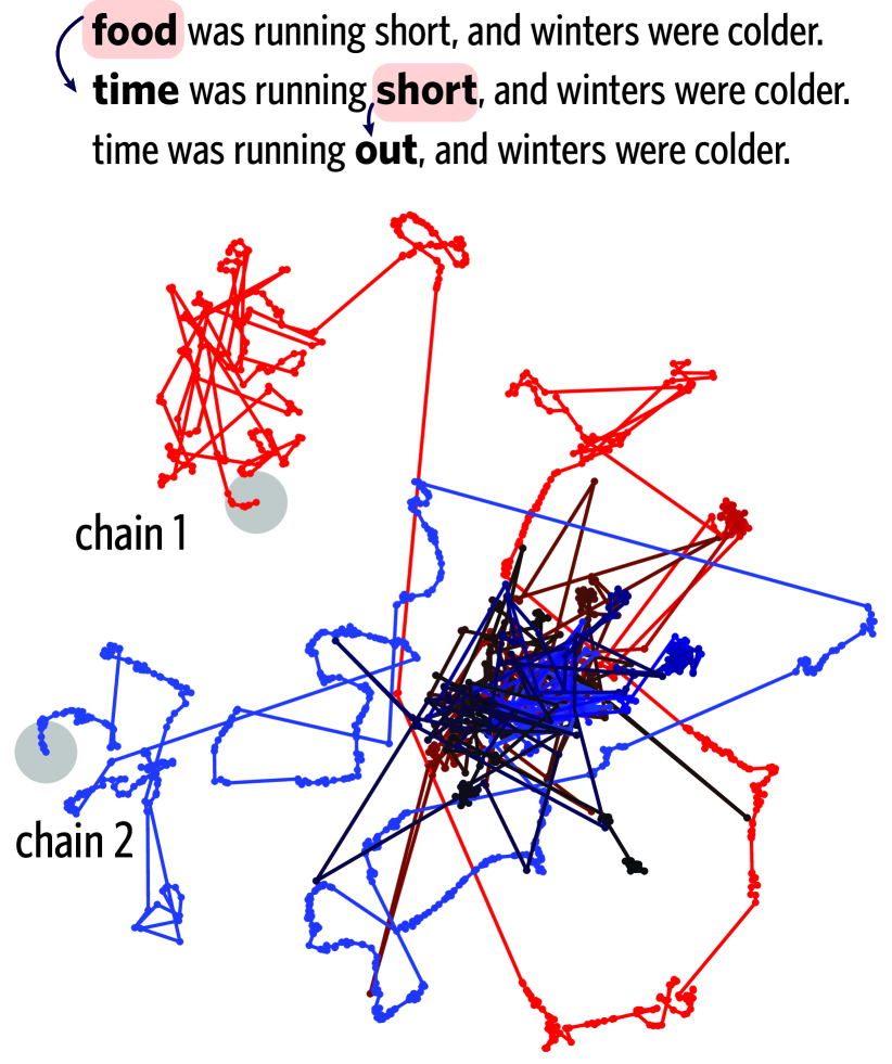
Figure 1: We use a serial reproduction method to probe BERT’s prior over possible sentences (visualization of reproduction chains obtained by running t-sne on sentence embeddings; chains are color-coded and fade to black across their burn-in period).

Type of unnaturalness		Example
word-level	morphological	Higher education school xur divided into six institutions.
phrase-level	syntactic	Swallowing hard, Verity stared at the these, desperately wanting to see if they congealed.
	semantic	The west section is a fig octagon.
		A private apartment with nothing but hot cooled water.
	predication	He already costumes his relationship with my mother carefully.
		Voices rapped on the incremental door.
sentence-level	out-of-context	Like a cataract, Horatius responds, “You are better than me.”
	self-contradictory	The newspaper is published weekly and biannually.
	pragmatic	She grew up with three sisters and ten sisters.
		It should apply between the extreme and the extreme.

Table 1: Examples of sentences sampled from BERT’s prior that received low naturalness ratings from our participants, including sources forms of unnaturalness like predicability or category errors (e.g. doors typically do not have the property of “incrementality”), semantic incoherence (“hot cooled water”), or contradictory constructions (especially for longer sentences). More examples can be found in table S2 and in the online supplement.

These deviations present a core theoretical and methodological puzzle for computational linguistics. How do we elicit and characterize the full prior that a particular model has learned over possible sentences in a language? A dominant approach has been to design benchmark suites that probe theoretically important aspects of the prior, and compare model behavior to human behavior on those tasks (e.g. Warstadt et al., 2020; Ettinger, 2020). Yet this approach can be restrictive and piecemeal: it is not clear ahead of time which tasks will be most diagnostic, and many sources of “weirdness” are not easily operationalized Kuribayashi et al. (2021).

A more holistic, bottom-up alternative is to directly examine samples from the model’s prior and compare them against those from human priors. However, many successful models do not explicitly expose this distribution, and many generation methods optimize the “best” sentences rather than theoretically meaningful or representative ones. For example, masked language models (MLMs) like BERT Devlin et al. (2018) are dependency networks Heckerman et al. (2000); Toutanova et al. (2003), trained to efficiently learn an independent collection of conditional distributions without enforcing consistency between them. In other words, these conditionals may not correspond to any coherent joint distribution at all, leading recent work to focus on other score-based sampling objectives Goyal et al. (2021).

Here, we explore the use of serial reproduction chains (see Fig. 1) to overcome these challenges. While a naive (pseudo-)Gibbs sampler is indeed problematic for MLMs, the literature on Generative Stochastic Networks (GSNs; Bengio et al., 2014) has formally shown that a simple algorithmic variant we call GSN sampling produces a stationary distribution that is, in fact, a unique and consistent estimator of the ground-truth joint distribution. Furthermore, while the independent conditionals learned by dependency networks may be arbitrarily inconsistent in theory, empirical work has found that these deviations tend to be negligible in practice, especially on larger datasets Heckerman et al. (2000); Neville and Jensen (2007). Thus, we argue that it is both theoretically and empirically justified to take these samples as uniquely representative of the model’s prior over language.

We begin in Section 2 by introducing the serial reproduction approach and clarifying the problem of re-constructing a joint distribution from a dependency network. We then validate that our chains are well-behaved (Section 3) and compare the statistics of samples from BERT’s prior to the lexical and syntactic statistics of its ground-truth training corpus to measure distributional similarity (Section 4). Finally, in Section 5, we present a large-scale behavioral study eliciting naturalness judgments from human speakers and identify features of the generated sentences which most strongly predict human ratings of “weirdness” (see Table 1). We find that GSN samples closely approximate the ground-truth distribution and are judged to be more natural than other methods, while also revealing areas of improvement that have been difficult to quantify with top-down benchmarks.

2 Approach

2.1 Serial reproduction

Our approach is inspired by serial reproduction games like Telephone, where an initial message is gradually relayed along a chain from one speaker to the next. At each step, the message is changed subtly as a result of noisy transmission and reconstruction, and the final version of the message often differs drastically from the first. This serial reproduction method, initially introduced to psychology by Bartlett (1932), has become an invaluable tool for revealing human inductive biases Xu and Griffiths (2010); Langlois et al. (2021); Sanborn et al. (2010); Harrison et al. (2020). Because reconstructing a noisy message is guided by the listener’s prior expectations, such chains eventually converge to a stationary distribution that is equivalent to the population’s prior, reflecting what people expect others to say Kalish et al. (2007); Griffiths and Kalish (2007); Beppu and Griffiths (2009). For example, Meylan et al. (2021) recently evaluated the ability of neural language models to predict the changes made to sentences by human participants at each step of a serial reproduction chain. Thus, while serial reproduction is commonly used to probe human priors, and to compare models against human data, it is not yet in wide use for probing the models themselves.

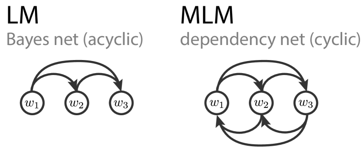
Figure 2: While autoregressive language models (LMs) are Bayes nets, masked language models (MLMs) are dependency networks with cyclic dependencies.

2.2 BERT as a dependency network

There has been considerable confusion in the recent literature over how to interpret the MLM objective used to train models like BERT, and how to interpret samples from such models. Wang and Cho (2019) initially observed that BERT was a Markov Random Field (MRF) and proposed a Gibbs sampler that iteratively masks and reconstructs different sites $k$ by sampling from the conditional given the tokens at all other sites $\hat{P}(w_{k}|w_{-k})$. As observed by Goyal et al. (2021), however, this procedure does not actually correspond to inference in the MRF. Unlike auto-regression language models (LMs) like GPT-3 Brown et al. (2020), which define an acyclic dependency graph (or Bayes net) from left-to-right, MLMs have cyclic dependencies (see Fig. 2) and are therefore usefully interpreted as dependency networks rather than Bayes networks Heckerman et al. (2000). Because dependency networks estimate independent conditionals, there is no guarantee that these conditionals are consistent (i.e. they may violate Bayes rule) and therefore do not represent a coherent joint distribution.

Still, it is possible to re-construct a joint distributions from these conditionals. For example, Heckerman et al. (2000) proved that if sites are visited in a fixed order, a (pseudo-)Gibbs chain similar to the one used by Wang and Cho (2019) does converge to a stationary distribution that is a well-formed joint. The problem is that different orders may yield different joint distributions, making it difficult to interpret any distributions as definitive. This ambiguity was resolved by the Generative Stochastic Network framework proposed by Bengio et al. (2014). Instead of visiting sites in a fixed order, a GSN sampler randomly chooses which site to visit at each step (with replacement), thus preserving aperiodicity and ergodicity. Specifically, this algorithm begins by initializing with a sequence $\{w_{1}^{0},\dots,w_{n}^{0}\}$. At each step $t$ of the chain, we randomly choose a site $k\in{1,\dots,n}$ to mask out, and we sample a new value $w_{k}^{t+1}$ from the conditional distribution $P(w_{k}|w_{-k}^{t})$ with the other $n-1$ sites fixed.

A key theorem of Bengio et al. (2013, 2014) proves that the stationary distribution arising from the GSN sampler defines a unique joint distribution, and furthermore, this stationary distribution is a consistent estimator of the ground-truth joint distribution. Importantly, this stationary distribution differs from the one given by the Metropolis-Hastings (MH) approach suggested by Goyal et al. (2021), which uses the GSN sampler as a proposal distribution but accepts or rejects proposals based on an energy-based pseudo-likelihood defined by the sum of the conditional scores at each location Salazar et al. (2020). This MH sampler instead converges to an implicit stationary distribution defined by the energy objective.

2.3 Mixture kernels

In practice, Markov chain sampling methods have many failure modes. Most prominently, because samples in the chains are not independent, it is challenging to guarantee convergence to a stationary distribution, and the chain is easily “stuck” in local regions of the sample space Gelman et al. (1992). Typically, samples from a burn-in period (e.g. the first $m$ epochs) are discarded to reduce dependence on the initial state, and a lag between samples (e.g. recording only every $l$ epochs) is introduced to reduce auto-correlation. However, the problem is particularly severe for language models like BERT where there are strong mutual dependencies between words at different sites. For example, once the chain reaches a tri-gram like ‘Papua New Guinea’, it is unlikely to change any single word while keeping the other words constant. To ensure ergodicity, we use a mixture kernel introducing a small constant probability ($\epsilon=0.001$) of returning to the initial distribution of [MASK] tokens on each epoch, allowing the chain to burn in again.

3 Validating the stationary distribution

In this section, we validate that the samples produced by our serial reproduction method are representative of the stationary prior distribution. More specifically, we consider two basic properties of the chain: convergence and independence. For these analyses, we consider samples from the pretrained bert-base-uncased model with 12 layers, 12 heads, and 110M parameters.

3.1 Convergence

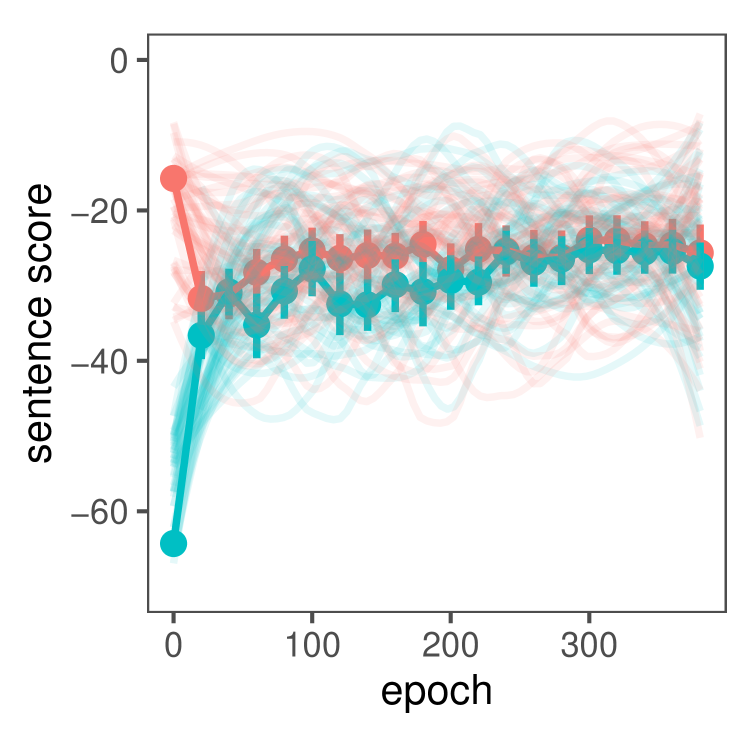
Figure S1: We examine the convergence time by initializing different chains at different classes of sentences (red is high probability under BERT’s energy function, blue is low probability). Faint lines show smoothed trajectories for individual chains and error bars are bootstrapped 95% confidence intervals across chains.

We begin by checking the convergence time for chains generated by GSN sampling. Theoretical bounds derived for serial reproduction chains give a convergence time of $n\log n$, where $n$ is the number of sites (see Rafferty et al., 2014). To check these convergence bounds in practice, we set $n=21$ and select 20 sentences from Wikipedia to serve as initial states, and run 10 chains initialized at each sentence. We ensured that half of these sentences have high initial probability (under BERT’s energy score) and half have low initial probability. We find that these distributions indeed begin to quickly mix in probability (see Figure S1). Because longer sentences may require a longer burn-in time, we conservatively set our burn-in window to $m=1000$ epochs for our subsequent experiments.

3.2 Independence

Second, we want to roughly ensure independence of samples, so that the statistics of our distribution of samples isn’t simply reflecting auto-correlation in the chain. For a worst-case analysis of a local minimum, suppose $P(w_{i}|w_{-i})<\delta$ $(0<\delta<1)$ for all $i\in[1,\dots,k]$, where $k$ is the sentence length in tokens. Then the probability of re-sampling the same sentence is roughly $<\delta^{k\cdot n}$ after $n$ epochs. We can solve for the number of epochs $n$ we need to bound the probability of re-sampling the exact same sentence under $\epsilon$ for a given worst-case $\delta$. For example, if $\delta=0.99$ and we want to ensure that the probability of re-sampling the same sentence is below a threshold $\epsilon=0.01$, then $n=47$ epochs will likely suffice. Ensuring complete turnover in the worst case scenario requires much longer lags, i.e. $[1-(1-\delta)^{k}]^{n}<\epsilon$.

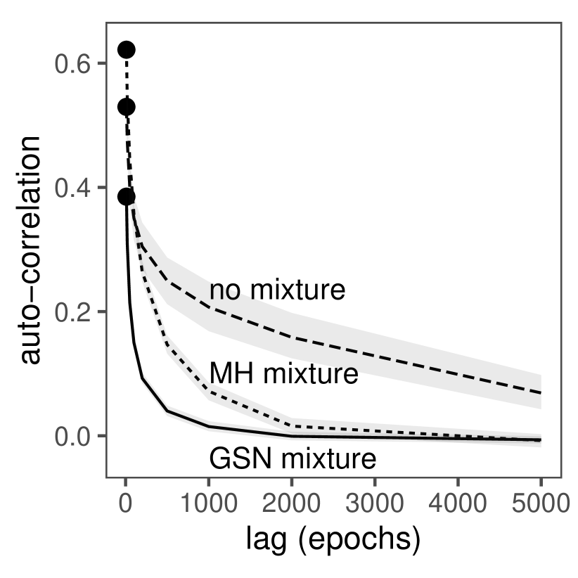
Figure S2: MCMC methods like GSN and MH sampling tend to get stuck in local regions with high auto-correlation. We find that a minimal autocorrelation is achievable with lower lag (500 epochs between samples) using a mixture kernel with a constant probability of resetting the chain. Error ribbons are 95% confidence intervals.

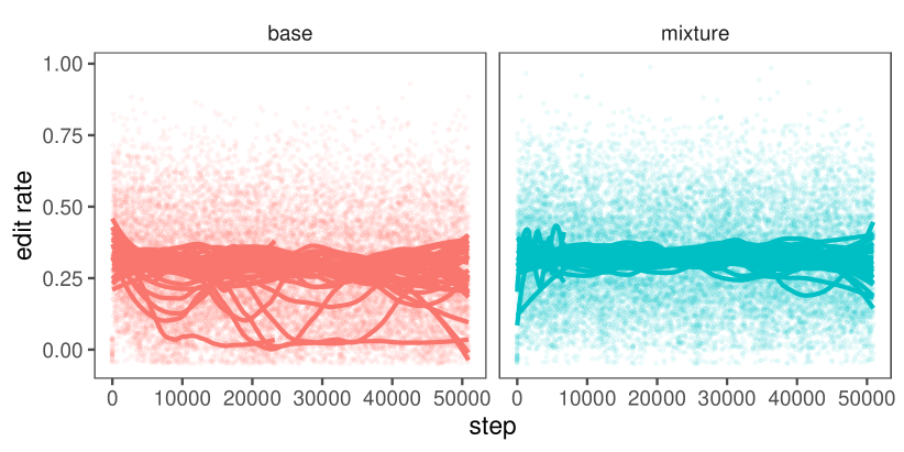
Figure S3: Without mixing in a constant probability of returning to the initial distribution, the GSN chain (and MH chain, not shown) goes through periods of stasis with low edit rates (red curves), contributing to high autocorrelations.

To evaluate the extent to which these cases arise in practice, we examine auto-correlation rates on longer chains (50,000 epochs). We calculate correlations between the energy scores at each epoch as a proxy for the state: when the chain gets stuck re-sampling the same sentence, the same scores appear repeatedly. We find that auto-correlation is generally high, but our mixture kernel prevents the worst local minima for both the MH chain Goyal et al. (2021) and our GSN chain (see Fig. S2), although we still found higher auto-correlation rates for the MH chain. To further examine these minima, we examined edit rates: the number of changes made to the sentence within an epoch. Without the mixture kernel, we observe long regions of consistently low edit rates (e.g. in some cases, 5000 epochs in a row of exactly the same sentence) which disappear under the mixture kernel (see Fig. S3).

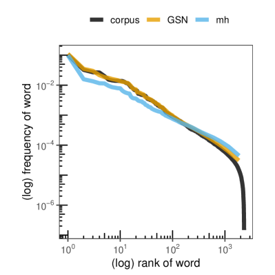
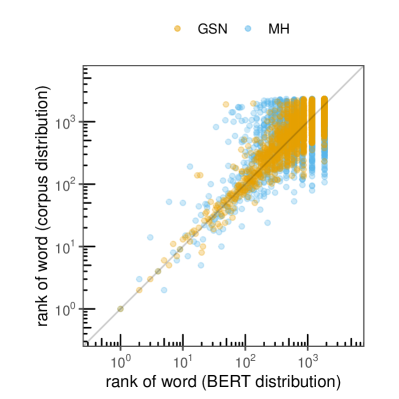
Figure 3: The lexical frequencies of our GSN samples (A) closely match the Zipfian distribution of the corpus and (B) closely correlate with the corresponding frequencies of the corpus distribution.

Based on these observations, we set the lag to $l=500$ epochs to maintain relatively high independence between samples.

4 Distributional comparisons

In this section, we examine the extent to which higher-order statistics of sentences from BERT’s prior are well-calibrated to the data it was trained on. This kind of comparison provides a richer sense of what the model has learned or failed to learn than traditional scalar metrics like perplexity Takahashi and Tanaka-Ishii (2017); Meister and Cotterell (2021); Takahashi and Tanaka-Ishii (2019); Pillutla et al. (2021).

4.1 Corpus preparation

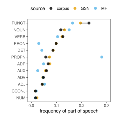
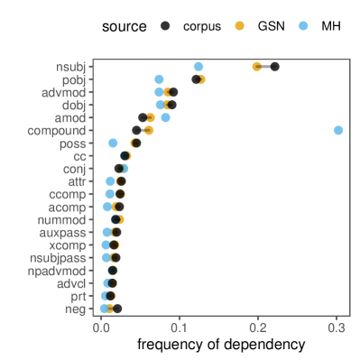
Figure 4: The relative frequencies of different parts of speech (left) and dependencies (right) in the ground-truth training corpora closely matched for GSN samples. In all cases, the GSN frequencies fell closer to the ground-truth than the MH frequencies.

The version of BERT we analyzed in the previous section was trained on a combination of two corpora: Wikipedia and BookCorpus. In order to make valid comparisons between human priors and machine priors, we needed to closely match BERT-generated sentences with a comparable subset of human-generated sentences from these combined corpora. There are two technical challenges we must overcome to ensure comparable samples, concerning the sentencizer and tokenizer steps.

First, because our unit of comparison is the sentence, we needed to control for any artifacts that may be induced by how we determine what sentences are (e.g. if our Wikipedia sentences were systematically split on abbreviations, skewing the distribution toward fragments). We therefore applied the same punkt sentencizer to create our distribution of Wikipedia sentences and to check our BERT samples for cases where the generated sequence contained multiple sentences or ended with a colon or semicolon.

Second, we needed a tokenizer that equates sentence length. Because bi-directional models like BERT operate over sequences of fixed length, all samples drawn from a single chain have the same number of tokens.

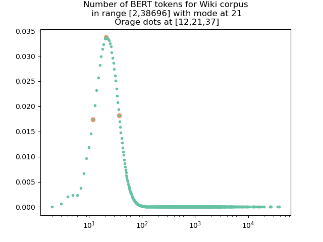
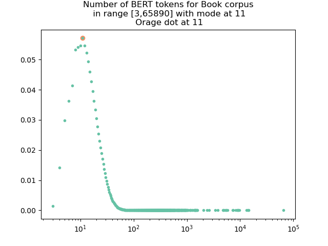
Figure S4: Empirical distribution of sentence lengths in Wikipedia and BookCorpus training corpora, after WordPiece tokenization. For our corpus comparisons, we selected the modal Wikipedia sentence length of 21 tokens and the modal BookCorpus length of 11 tokens. For our human judgment experiment, we included baseline sentences only from Wikipedia for shorter (12 tokens) and longer sentences (37 tokens), with roughly equal prevalence in the corpus (orange dots).

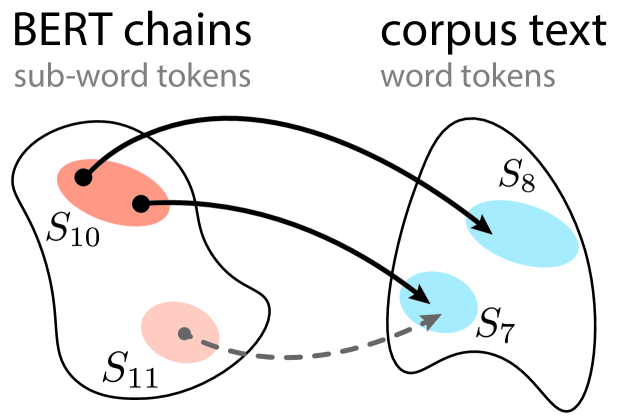
Figure S5: There is a misalignment between the space of sentences obtainable by a BERT chain of a fixed token length (in sub-word tokens) and natural language sentences of a fixed length (in words). We consider the distribution of corpus sentences that are obtainable from a fixed-length BERT chain, which may decode to different lengths in natural text (black arrows).

Critically, however, BERT chains are defined over sequences of WordPiece tokens, so once these sequences are decoded back into natural language text, they may yield sentences of varying length, depending on how the sub-word elements are combined together (see Fig. S5). We solve this alignment problem by using the WordPiece tokenizer to extract sentences of fixed sub-word token length from our text corpora, yielding equivalence classes of corpus sentences that are all tokenized to the same number of WordPiece tokens. We ran GSN and MH chains over sentences of $n=11$ tokens, representing the modal lengths of sentences in BookCorpus (see Fig. S4). We obtained 5,000 independent sentences from each sampling method after applying our conservative burn-in and lag, and combined the Wikipedia and BookCorpus sentences together into a single corpus that is representative of BERT’s training regime.

4.2 Lexical distributions

We begin by comparing the lexical frequency statistics of our samples from BERT against the ground-truth corpus statistics. First, we note that the relationship between rank and frequency of tokens in the GSN sampling matches the Zipfian distribution of its training corpus better than those produced by MH sampling (see Fig. 3A). However, it is possible to produce the same overall distribution without matching the empirical frequencies of individual words. We next examined the respective ranks of each word across the two distributions. Overall, the word ranks in the GSN samples had a strong Spearman rank correlation of $r=0.75$ with the word ranks in the ground-truth corpus; the MH samples had a significantly lower correlation of $r=0.48$ (Pearson $z=17,p<0.001$, Fig  3B). Most disagreements lay in the tails where frequency estimates are particularly poor (e.g. many words only appeared once in our collection of samples). Indeed, among words with greater than 10 occurrences, the correlation improved to $r=0.83$ for GSN and $r=0.65$ for MH.

To understand this relationship further, we conducted an error analysis of lexical items which were systematically over- or under-produced by BERT relative to its training corpus. We found that certain punctuation tokens (e.g. parentheses) were over-represented in both the GSN samples and the MH samples, while contractions like ’s and ’d were under-represented. The MH samples specifically over-produced proper names such as Nina and Jones. Finally, due to the use of sub-word representations, we found a long tail of morphologically complex words that did not appear at all in the training corpus (e.g. names like Kyftenberg or Streckenstein and seemingly invented scientific terms like lymphoplasmic, neopomphorus, or pyranolamines).

4.3 Syntactic distributions

While the lexical distributions were overall well-matched for GSN samples, our error analysis suggested potential structure in the deviations. In other words, entire grammatical constructions may be over- or under-represented, not just particular words. To investigate these patterns, we used the spacy library to extract the parts of speech and dependency relations that are present within each sentence. We are then able to examine, in aggregate, whether certain classes of constructions are disproportionately responsible for deviations. Our findings are shown in Fig. 4. Overall, the distributions are close, but several areas of misalignment emerge. For parts of speech, we observe that the GSN sampler is slightly over-producing nouns (and proper nouns) while under-producing verbs and prepositions. We also observe that it is over-producing noun-related dependencies (e.g. compound nouns and appositional modifiers, which are noun phrases modifying other noun phrases, as in “Bill, my brother, visited town”). This pattern suggests that BERT’s prior may be skewed toward (simpler) noun phrases while neglecting more complex constructions.

4.4 Sentence complexity

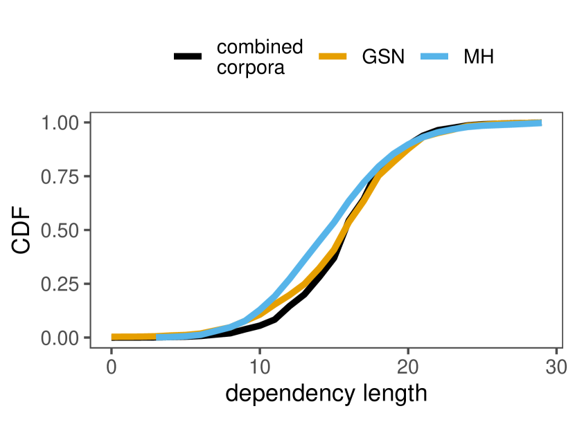
Figure 5: Cumulative probability distribution of dependency lengths across sentences from BERT chains and from the training corpus.

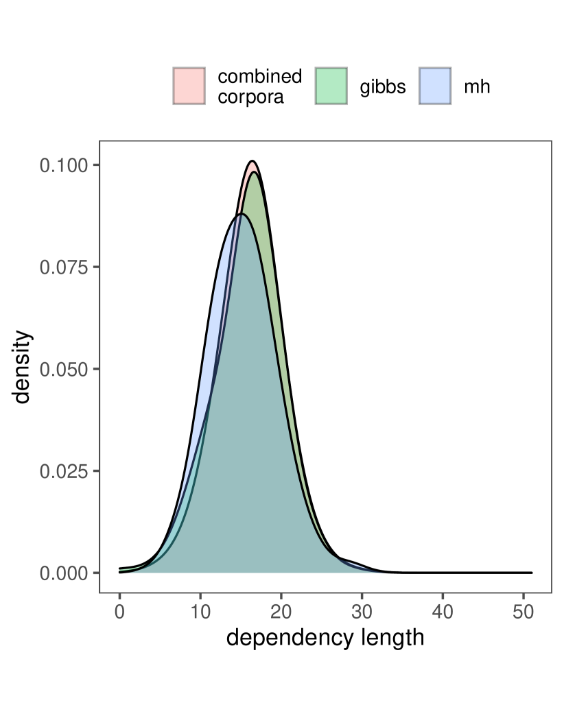
Figure S6: Dependency distances are similar for sentences sampled from BERT’s prior and sentences from its training corpus, but the BERT distribution is more bimodal and tends to skew simpler.

One hypothesis raised by comparing distributions of syntactic features is that BERT may be regularizing the complex structure of its input toward simpler constructions. To test this hypothesis, we operationalize syntactic complexity using a measure known as the average dependency length of a sentence Futrell et al. (2015); Grodner and Gibson (2005). This measure captures the (linear) distance between syntactically related words, which increases with more complex embedded phrase structures. We found that the distribution of dependency distances in the sentences produced by GSN sampling is overall more similar to those in its training corpus than the MH (Fig. 5), although closer analysis suggests it is still skewed slightly simpler (see Fig. S6).

5 Human judgments

Finally, while our corpus comparisons highlighted particular ways in which samples from BERT’s prior were well-calibrated to the high-level statistics of its training distribution, it is unclear whether these agreements or deviations ‘matter’ in terms of naturalness. In this section, we elicit human naturalness judgments in order to provide a more holistic measure of potential ‘weirdness’ with BERT sentences.

5.1 Experimental methods

We recruited 1016 fluent English speakers on the Prolific platform and asked them to judge the naturalness of 4040 unique sentences from three length classes: short (11 tokens), medium (21 tokens), and long (37 tokens). 1675 of these sentences were from the stationary state of the different chains, 2339 were from the burn-in phase (i.e. $<1000$ epochs), and the remainder were baseline sentences (149 from Wikipedia, 48 from a 5-gram model, and 42 from an LSTM model; see Appendix for details). Each participant was shown a sequence of 25 sentences in randomized order, balanced across different properties of the stimulus set. On each trial, one of these sentences appeared with a slider ranging from 0 (“very weird”) to 100 (“completely natural”). After excluding 8 participants who failed the attention check (i.e. failed to rate a scrambled sentence below the midpoint of the scale and a human-generated sentence above the midpoint), we were left with an average of 7.3 responses per sentence.

5.2 Behavioral results

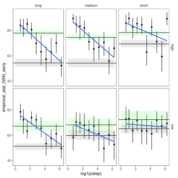
Figure S7: Sentences gradually drift away from the initial distribution across the burn-in period. Light green region represents the 95% confidence interval for the mean naturalness of Wikipedia sentences while grey region represents the same interval around the stationary distribution of the converged chain. Top row represents chains that are initialized at high-probability states, while bottom row is initialized in low-probability states.

We begin by comparing the naturalness of sentences from the stationary GSN distribution to other baselines (see Fig. 6), using a linear regression model predicting trial-by-trial judgments as a function of categorical variables encoding sentence length (short, medium, long) and the source of the sentence (Wikipedia, GSN, MH, LSTM, or n-gram). First, we find that the naturalness of sentences from GSN declines by 14 points at longer sentence lengths, $p<0.001$, while the naturalness of Wikipedia sentences is unaffected by length (interaction term, $p<0.001$), consistent with results reported by Ippolito et al. (2020). Furthermore, among short sentences, where we included additional baselines, we find that GSN sentences tend to be rated as slightly less natural than sentences from Wikipedia (+10 points, $p<0.001)$ but more natural than those produced by an n-gram model (-52 points, $p<0.001$), LSTM model (-25 points, $p<0.001$); or MH sampling from the same BERT conditionals (-15 points, $p<0.001$; see Table S1). MH samples also deteriorate significantly in naturalness for longer sentences compared to GSN samples ($p<0.001$). Finally, we examine naturalness ratings across the the burn-in period, finding that ratings decline steadily across the board as the chain takes additional steps (linear term: $t(7297)=-12.4,p<0.001$), suggesting gradual deviation away from the initial distribution of Wikipedia sentences toward the stationary distribution (shown as the green and grey regions, respectively, in Fig. S7).

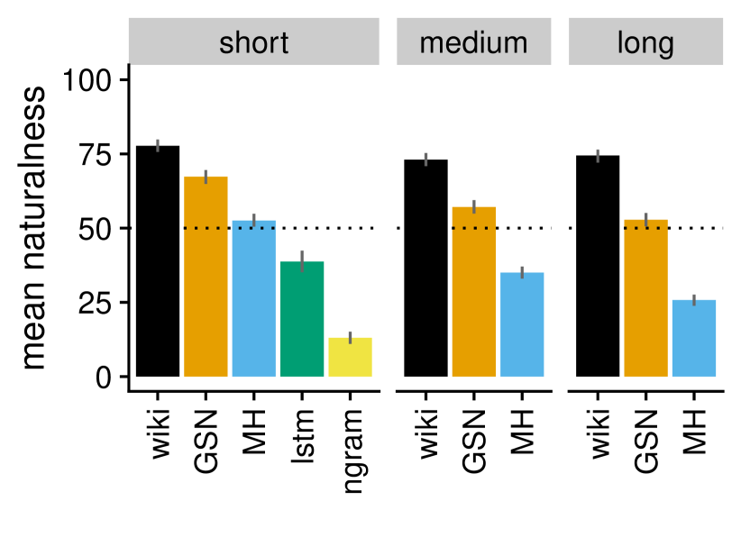
Figure 6: Empirical naturalness ratings elicited from the stationary GSN distribution, compared to different baselines at different sentence lengths. Error bars are bootstrapped 95% CIs.

5.3 Predicting naturalness

Given that sentences from the stationary GSN distribution are judged to be less natural than human-generated sentences overall, we are interested in explaining why. Which properties of these sentences make them sound strange? We approach this problem by training a regression model to predict human judgments from attributes of each sentence. We include all part of speech tag counts and dependency counts, as well as the sentence probability scored under BERT, and the sentence length. We use a cross-validated backwards feature selection procedure to select the most predictive set of these features for a linear regression Kuhn and Johnson (2013).

The best-fitting model used 26 features and achieved an (adjusted) $R^{2}=0.21$. The only features associated with significantly lower ratings were the use of adpositions (e.g. before, after) and coordinating conjunctions. Importantly, we found that including a categorical variable of corpus (i.e. Wikipedia vs. GSN) significantly improved model fit even after controlling for all other features, $\chi^{2}(1)=7135,p<0.001$, suggesting that sources of “weirdness” are not being captured by typical statistics. We show some of these low-naturalness sentences in Table 1 and S2.

6 Discussion

6.1 Probing through generation

A core idea of our serial reproduction approach is to use generation as a window into a model’s prior over language. While a variety of metrics and techniques have been proposed to quantify the “quality” of generation, especially in the domains of open-ended text generation and dialogue systems Caccia et al. (2020); Li et al. (2020); Guidotti et al. (2018); Celikyilmaz et al. (2020), these metrics have typically been applied to compare specific generation algorithms and operationalize specific pitfalls, such as incoherence, excess repetition, or lack of diversity. Consequently, it has been difficult to disentangle the extent to which deviations resulting from generations are an artifact of specific decoding algorithms (e.g. greedy search vs. beam search) or run deeper, into the prior itself. For the purposes of probing, we suggest that it is important to ask not only how to generate the highest-scoring sentences but how to generate sentences that may be interpreted as representative of the model’s prior, as formal results on GSNs have effectively provided.

6.2 GSN vs. energy-based objectives

We found that the prior distribution yielded by the GSN sampler more closely approximated the lexical and syntactic distributions of the ground-truth corpus and also sounded more “natural” to humans than the samples yielded by MH. These results are in contrast to findings by Goyal et al. (2021), showing that MH produced high-quality BLEU scores on a Machine Translation (MT) task compared to a degenerate (pseudo-)Gibbs sampler. There are several possible reasons for this discrepancy. One possibility may be task-specific: while we focused on unconditional generation, Goyal et al. (2021) focused on a neural machine translation (MT) task, where sentence generation was always conditioned on a high-quality source text and thus remained within a constrained region of sentence space. Another possibility is that we ran substantially longer chains (50,000 epochs compared to only 33 epochs) and the pitfalls of MH sampling only emerged later in the chain.

More broadly, our corpus comparisons and human evaluations suggest serious limitations of simple “quality” metrics like energy values. We found that the best-scoring states were often degenerate local minima with mutually supporting n-grams (such as repetitive phases and names like “Papua New Guinea”). Indeed, there was only a loose relationship between energy scores and participants’ judgments in our study, with many poorer-scoring sentences judged to be more natural than better-scoring sentences (e.g. overall, the distribution of Wikipedia sentences tended to be much lower-scoring under the energy function despite being rated as more natural). We empirically validated that the stationary distribution of the GSN chain successfully approximates even higher-order statistics of the ground-truth corpus, suggesting that the raw conditionals of the dependency network may implicitly acquire the joint distribution, without requiring guarantees of consistency.

6.3 Other architectures

Serial reproduction methods are particularly useful for probing models that do not directly generate samples from their prior. For auto-regressive models like GPT-2, these samples are obtained more directly by running the model forward (and, indeed, ancestral sampling produces text that better balances the precision-recall tradeoff than other algorithms; Pillutla et al., 2021). While we focused on BERT, this method may be particularly useful for encoder-decoder architectures like BART Lewis et al. (2020) which more closely resemble the human Telephone Game task, requiring full reconstruction of the entire sentence from noisy input rather than reconstruction of a single missing word. Indeed, these architectures may overcome an important limitation of serial reproduction with BERT: because these chains operate over a fixed sequence length, the resulting prior is not over all of language but only over sentences with the given number of WordPiece tokens. Finally, while we focused on unconditional generation, the GSN sampler also generalizes straightforwardly to conditional generation, where a subset of sites are fixed and the masked site is chosen from the remaining set.

6.4 Conclusions

Serial reproduction paradigms have been central for exposing human priors in the cognitive sciences. In this paper, we drew upon the theory of iterated learning and of Generative Stochastic Networks (GSNs) to expose the priors of large neural language models, which are often similarly inscrutable. We hope future work will consider other points of contact between these areas and draw more extensively from the theory developed to understand dependency networks. More broadly, as language models become increasingly adaptive and deployed in increasingly unconstrained settings, bottom-up probing has the potential to reveal a broader spectrum of “weirdness” than top-down evaluative benchmarks.

Appendix A: Baseline details

Wikipedia sentences were randomly selected from the full sentencized corpus English Wikipedia that tokenized to 12, 21, and 37 WordPiece tokens for the short, medium, and long conditions, respectively. These sentences were also chosen to span a broad range of sentence probabilities under BERT (i.e. $\log P(p_{1},\dots,p_{n})=\sum_{k}\log P(p_{k}|p_{-k})$).

For our ngram baseline, we trained a 5-gram model with Kneser-Ney smoothing Kneser and Ney (1995) on English Wikipedia using the kenlm library Heafield (2011), and generated sentences of length 10 by sampling from the resulting conditional distributions. Because this model stripped punctuation, and was therefore unable to emit an “end of sentence” token, we expected it to serve as a lower bound on the naturalness scale.

For our LSTM baseline, we used the network pre-trained by Gulordava et al. (2018) on English Wikipedia. This model was trained to emit an end of sentence (<eos>) token, allowing us to rejection sample to obtain sentences that were exactly 10 words long with no unknown words (i.e. <unk> tokens). Because it was not trained with a <start> token, however, we needed to initialize it with the initial word of the sentence. We randomly selected this initial word from a small set of common sentence openers (e.g. the, a, it, his, her). As a result of our initial token selection, this model does not precisely sample from its true prior over sentences. Thus, it is best viewed as another baseline of sentences rather than as a careful architectural comparison.

Because we were asking participants to judge the naturalness of complete sentences, we did not want to include samples which clearly violated sentencehood, as these would not be informative (e.g. fragments from Wikipedia that were incorrectly sentencized and ended with an abbreviation, bibliographic text like “korsakov (1976) r.s.,” or table markdown with pipes like “$|$ a $|$ b $|$”). We automatically removed any sentences containing pipes or ending with colons or semicolons, as these were associated with sentencizer inconsistency, as well as sequences that contained multiple sentences (according to our sentencizer). Finally, the authors took a manual pass to exclude other non-sentential fragments from the stimulus set.

	term	estimate	std.error	statistic	p.value
1	(Intercept)	67.33	1.14	59.08	$<0.001$
2	short vs. long (GSN)	-14.49	1.60	-9.08	$<0.001$
3	short vs. medium (GSN)	-10.21	1.60	-6.39	$<0.001$
5	GSN vs. LSTM (short)	-28.60	2.04	-14.05	$<0.001$
6	GSN vs. MH (short)	-14.76	1.59	-9.26	$<0.001$
7	GSN vs. ngram (short)	-54.26	2.00	-27.07	$<0.001$
8	GSN vs. wiki (short)	10.40	1.70	6.13	$<0.001$
13	interaction (short vs. long; GSN vs. MH)	-12.31	2.23	-5.51	$<0.001$
14	interaction (short vs. medium; GSN vs. MH)	-7.33	2.23	-3.29	$<0.001$
17	interaction (short vs. long; GSN vs. wiki)	11.22	2.39	4.70	$<0.001$
18	interaction (short vs. medium; GSN vs. wiki)	5.56	2.37	2.35	0.02

Table S1: Fixed effect estimates for regression on human scores. Length class and source are dummy coded with short lengths and GSN as baselines.

Appendix B: Corpus details

We downloaded cleaned Wikipedia data provided by GluonNLP (https://github.com/dmlc/gluon-nlp/tree/master/scripts/datasets/pretrain_corpus), and BookCorpus data from HuggingFace Datasets (https://huggingface.co/datasets/bookcorpus).

types of unnaturalness		examples
character-level		He preened on a レ drink of copper.
phrase-level	semantic	The little wattled songbird, also called the Chink Warbler, Orange Garver or Quickcumber is a socially luscious and habituated bird species.
sentence-level	construction	There were two hours before he made the walk.
	out-of-context word	No need to focus on bicycling.
	self-contradictory	The symbols $(\cdot\cdot\cdot)$ read as $(\cdot\cdot\cdot)$ and $(\cdot)$ are written as $(\cdot\cdot\cdot\cdot\cdot)$ , not as $(\cdot)$.
	repetition	The college of arts and sciences, adjacent to the business school, is majoring in business.
		He saw Cronus and Cronus, Cronus and James Cronus he saw Cronus and Cronus and Cronus and Cronus Cronus when he saw Cronus.

Table S2: More examples of sentences from BERT’s prior with low naturalness ratings.

References

- Bartlett (1932) Frederic Charles Bartlett. 1932. Remembering: A study in experimental and social psychology. Cambridge University Press.
- Bender et al. (2021) Emily M Bender, Timnit Gebru, Angelina McMillan-Major, and Shmargaret Shmitchell. 2021. On the dangers of stochastic parrots: Can language models be too big? In Proceedings of the 2021 ACM Conference on Fairness, Accountability, and Transparency, pages 610–623.
- Bengio et al. (2014) Yoshua Bengio, Eric Laufer, Guillaume Alain, and Jason Yosinski. 2014. Deep generative stochastic networks trainable by backprop. In International Conference on Machine Learning, pages 226–234. PMLR.
- Bengio et al. (2013) Yoshua Bengio, Li Yao, Guillaume Alain, and Pascal Vincent. 2013. Generalized denoising auto-encoders as generative models. Advances in neural information processing systems, 26.
- Beppu and Griffiths (2009) Aaron Beppu and Thomas Griffiths. 2009. Iterated learning and the cultural ratchet. In Proceedings of the Annual Meeting of the Cognitive Science Society, volume 31.
- Braverman et al. (2020) Mark Braverman, Xinyi Chen, Sham Kakade, Karthik Narasimhan, Cyril Zhang, and Yi Zhang. 2020. Calibration, entropy rates, and memory in language models. In International Conference on Machine Learning, pages 1089–1099. PMLR.
- Brown et al. (2020) Tom B Brown, Benjamin Mann, Nick Ryder, Melanie Subbiah, Jared Kaplan, Prafulla Dhariwal, Arvind Neelakantan, Pranav Shyam, Girish Sastry, Amanda Askell, et al. 2020. Language models are few-shot learners. Advances in Neural Information Processing Systems, 34.
- Caccia et al. (2020) Massimo Caccia, Lucas Caccia, William Fedus, Hugo Larochelle, Joelle Pineau, and Laurent Charlin. 2020. Language GANs falling short. International Conference on Learning Representations.
- Caliskan et al. (2017) Aylin Caliskan, Joanna J Bryson, and Arvind Narayanan. 2017. Semantics derived automatically from language corpora contain human-like biases. Science, 356(6334):183–186.
- Celikyilmaz et al. (2020) Asli Celikyilmaz, Elizabeth Clark, and Jianfeng Gao. 2020. Evaluation of text generation: A survey. arXiv preprint arXiv:2006.14799.
- Clark et al. (2021) Elizabeth Clark, Tal August, Sofia Serrano, Nikita Haduong, Suchin Gururangan, and Noah A. Smith. 2021. All that’s ‘human’ is not gold: Evaluating human evaluation of generated text. In Proceedings of the 59th Annual Meeting of the Association for Computational Linguistics., pages 7282–7296.
- Dasgupta et al. (2020) Ishita Dasgupta, Demi Guo, Samuel J Gershman, and Noah D Goodman. 2020. Analyzing machine-learned representations: A natural language case study. Cognitive Science, 44(12):e12925.
- Devlin et al. (2018) Jacob Devlin, Ming-Wei Chang, Kenton Lee, and Kristina Toutanova. 2018. BERT: Pre-training of deep bidirectional transformers for language understanding. In Proceedings of NAACL-HLT.
- Ettinger (2020) Allyson Ettinger. 2020. What bert is not: Lessons from a new suite of psycholinguistic diagnostics for language models. Transactions of the Association for Computational Linguistics, 8:34–48.
- Futrell et al. (2015) Richard Futrell, Kyle Mahowald, and Edward Gibson. 2015. Large-scale evidence of dependency length minimization in 37 languages. Proceedings of the National Academy of Sciences, 112(33):10336–10341.
- Garg et al. (2018) Nikhil Garg, Londa Schiebinger, Dan Jurafsky, and James Zou. 2018. Word embeddings quantify 100 years of gender and ethnic stereotypes. Proceedings of the National Academy of Sciences, 115(16):E3635–E3644.
- Gelman et al. (1992) Andrew Gelman, Donald B Rubin, et al. 1992. Inference from iterative simulation using multiple sequences. Statistical science, 7(4):457–472.
- Goyal et al. (2021) Kartik Goyal, Chris Dyer, and Taylor Berg-Kirkpatrick. 2021. Exposing the implicit energy networks behind masked language models via Metropolis–Hastings. arXiv preprint arXiv:2106.02736.
- Griffiths and Kalish (2007) Thomas L Griffiths and Michael L Kalish. 2007. Language evolution by iterated learning with Bayesian agents. Cognitive Science, 31(3):441–480.
- Grodner and Gibson (2005) Daniel Grodner and Edward Gibson. 2005. Consequences of the serial nature of linguistic input for sentenial complexity. Cognitive Science, 29(2):261–290.
- Guidotti et al. (2018) Riccardo Guidotti, Anna Monreale, Salvatore Ruggieri, Franco Turini, Fosca Giannotti, and Dino Pedreschi. 2018. A survey of methods for explaining black box models. ACM computing surveys (CSUR), 51(5):1–42.
- Gulordava et al. (2018) Kristina Gulordava, Piotr Bojanowski, Edouard Grave, Tal Linzen, and Marco Baroni. 2018. Colorless green recurrent networks dream hierarchically. In Proceedings of NAACL-HLT, page 1195–1205.
- Harrison et al. (2020) Peter Harrison, Raja Marjieh, Federico Adolfi, Pol van Rijn, Manuel Anglada-Tort, Ofer Tchernichovski, Pauline Larrouy-Maestri, and Nori Jacoby. 2020. Gibbs sampling with people. Advances in Neural Information Processing Systems, 33.
- Hawkins et al. (2020) Robert Hawkins, Takateru Yamakoshi, Thomas Griffiths, and Adele Goldberg. 2020. Investigating representations of verb bias in neural language models. In Proceedings of the 2020 Conference on Empirical Methods in Natural Language Processing (EMNLP), pages 4653–4663.
- Heafield (2011) Kenneth Heafield. 2011. Kenlm: Faster and smaller language model queries. In Proceedings of the sixth workshop on statistical machine translation, pages 187–197.
- Heckerman et al. (2000) David Heckerman, David Maxwell Chickering, Christopher Meek, Robert Rounthwaite, and Carl Kadie. 2000. Dependency networks for inference, collaborative filtering, and data visualization. Journal of Machine Learning Research, 1(Oct):49–75.
- Holtzman et al. (2019) Ari Holtzman, Jan Buys, Li Du, Maxwell Forbes, and Yejin Choi. 2019. The curious case of neural text degeneration. International Conference on Learning Representations.
- Ippolito et al. (2020) Daphne Ippolito, Daniel Duckworth, Chris Callison-Burch, and Douglas Eck. 2020. Automatic detection of generated text is easiest when humans are fooled. In Proceedings of the 58th Annual Meeting of the Association for Computational Linguistics, pages 1808–1822.
- Kalish et al. (2007) Michael L Kalish, Thomas L Griffiths, and Stephan Lewandowsky. 2007. Iterated learning: Intergenerational knowledge transmission reveals inductive biases. Psychonomic Bulletin & Review, 14(2):288–294.
- Kneser and Ney (1995) Reinhard Kneser and Hermann Ney. 1995. Improved backing-off for m-gram language modeling. In 1995 international conference on acoustics, speech, and signal processing, volume 1, pages 181–184. IEEE.
- Kuhn and Johnson (2013) Max Kuhn and Kjell Johnson. 2013. An introduction to feature selection. In Applied predictive modeling, pages 487–519. Springer.
- Kuribayashi et al. (2021) Tatsuki Kuribayashi, Yohei Oseki, Takumi Ito, Ryo Yoshida, Masayuki Asahara, and Kentaro Inui. 2021. Lower perplexity is not always human-like. In Proceedings of the 59th Annual Meeting of the Association for Computational Linguistics, pages 5203–5217.
- Langlois et al. (2021) Thomas A Langlois, Nori Jacoby, Jordan W Suchow, and Thomas L Griffiths. 2021. Serial reproduction reveals the geometry of visuospatial representations. Proceedings of the National Academy of Sciences, 118(13).
- Lewis et al. (2020) Mike Lewis, Yinhan Liu, Naman Goyal, Marjan Ghazvininejad, Abdelrahman Mohamed, Omer Levy, Veselin Stoyanov, and Luke Zettlemoyer. 2020. BART: Denoising sequence-to-sequence pre-training for natural language generation, translation, and comprehension. In Proceedings of the 58th Annual Meeting of the Association for Computational Linguistics, pages 7871–7880.
- Li et al. (2020) Margaret Li, Stephen Roller, Ilia Kulikov, Sean Welleck, Y-Lan Boureau, Kyunghyun Cho, and Jason Weston. 2020. Don’t say that! making inconsistent dialogue unlikely with unlikelihood training. In Proceedings of the 58th Annual Meeting of the Association for Computational Linguistics, pages 4715–4728.
- Linzen and Baroni (2021) Tal Linzen and Marco Baroni. 2021. Syntactic structure from deep learning. Annual Review of Linguistics, 7(1).
- McAllester (2019) David McAllester. 2019. A consistency theorem for BERT. Retrieved November 1, 2021 from https://machinethoughts.wordpress.com/2019/07/14/a-consistency-theorem-for-bert/.
- Meister and Cotterell (2021) Clara Meister and Ryan Cotterell. 2021. Language model evaluation beyond perplexity. In Proceedings of the 59th Annual Meeting of the ACL, pages 5328–5339.
- Meylan et al. (2021) Stephan C Meylan, Sathvik Nair, and Thomas L Griffiths. 2021. Evaluating models of robust word recognition with serial reproduction. Cognition, 210:104553.
- Neville and Jensen (2007) Jennifer Neville and David Jensen. 2007. Relational dependency networks. Journal of Machine Learning Research, 8(3):653–692.
- Pillutla et al. (2021) Krishna Pillutla, Swabha Swayamdipta, Rowan Zellers, John Thickstun, Sean Welleck, Yejin Choi, and Zaid Harchaoui. 2021. Mauve: Measuring the gap between neural text and human text using divergence frontiers. Advances in Neural Information Processing Systems, 34.
- Rafferty et al. (2014) Anna N Rafferty, Thomas L Griffiths, and Dan Klein. 2014. Analyzing the rate at which languages lose the influence of a common ancestor. Cognitive Science, 38(7):1406–1431.
- Salazar et al. (2020) Julian Salazar, Davis Liang, Toan Q. Nguyen, and Katrin Kirchhoff. 2020. Masked language model scoring. In Proceedings of the 58th Annual Meeting of the Association for Computational Linguistics, pages 2699–2712.
- Sanborn et al. (2010) Adam N Sanborn, Thomas L Griffiths, and Richard M Shiffrin. 2010. Uncovering mental representations with Markov chain Monte Carlo. Cognitive psychology, 60(2):63–106.
- Shane (2019) Janelle Shane. 2019. You look like a thing and I love you. Hachette UK.
- Takahashi and Tanaka-Ishii (2017) Shuntaro Takahashi and Kumiko Tanaka-Ishii. 2017. Do neural nets learn statistical laws behind natural language? PloS one, 12(12):e0189326.
- Takahashi and Tanaka-Ishii (2019) Shuntaro Takahashi and Kumiko Tanaka-Ishii. 2019. Evaluating computational language models with scaling properties of natural language. Computational Linguistics, 45(3):481–513.
- Tenney et al. (2019) Ian Tenney, Dipanjan Das, and Ellie Pavlick. 2019. BERT rediscovers the classical NLP pipeline. In Proceedings of ACL, page 4593–4601.
- Toutanova et al. (2003) Kristina Toutanova, Dan Klein, Christopher D Manning, and Yoram Singer. 2003. Feature-rich part-of-speech tagging with a cyclic dependency network. In Proceedings of the 2003 Human Language Technology Conference of the North American Chapter of the Association for Computational Linguistics, pages 252–259.
- Wang and Cho (2019) Alex Wang and Kyunghyun Cho. 2019. BERT has a mouth, and it must speak: BERT as a Markov Random Field language model. In Proceedings of the Workshop on Methods for Optimizing and Evaluating Neural Language Generation (NeuralGen), page 30–36.
- Warstadt et al. (2020) Alex Warstadt, Alicia Parrish, Haokun Liu, Anhad Mohananey, Wei Peng, Sheng-Fu Wang, and Samuel R Bowman. 2020. Blimp: The benchmark of linguistic minimal pairs for english. Transactions of the Association for Computational Linguistics, 8:377–392.
- Warstadt et al. (2019) Alex Warstadt, Amanpreet Singh, and Samuel R Bowman. 2019. Neural network acceptability judgments. Transactions of the Association for Computational Linguistics, 7:625–641.
- Xu and Griffiths (2010) Jing Xu and Thomas L Griffiths. 2010. A rational analysis of the effects of memory biases on serial reproduction. Cognitive psychology, 60(2):107–126.