An optimal scheduled learning rate for a randomized Kaczmarz algorithm

Abstract.

We study how the learning rate affects the performance of a relaxed randomized Kaczmarz algorithm for solving $Ax\approx b+\varepsilon$, where $Ax=b$ is a consistent linear system and $\varepsilon$ has independent mean zero random entries. We derive a learning rate schedule which optimizes a bound on the expected error that is sharp in certain cases; in contrast to the exponential convergence of the standard randomized Kaczmarz algorithm, our optimized bound involves the reciprocal of the Lambert-$W$ function of an exponential.

1. Introduction and main result

1.1. Introduction

Let $A$ be an $m\times n$ matrix and $Ax=b$ be a consistent linear system of equations. Suppose that $\tilde{b}$ is a corrupted version of $b$ defined by

$$\tilde{b}=b+\varepsilon,$$ (1)

where $\varepsilon$ has independent mean zero random entries. Given an initial vector $x_{0}$, we consider the relaxed Kaczmarz algorithm

$$x_{k+1}=x_{k}+\alpha_{k}\frac{\tilde{b}_{i_{k}}-\langle a_{i_{k}},x_{k}\rangle}{\|a_{i_{k}}\|^{2}}a_{i_{k}},$$ (2)

where $\alpha_{k}$ is the learning rate (or relaxation parameter), $a_{i}$ is the $i$-th row of $A$, $\tilde{b}_{i}$ is the $i$-th element of $\tilde{b}$, $i_{k}$ is the row index for iteration $k$, $\langle\cdot,\cdot\rangle$ is the $\ell^{2}$-inner product, and $\|\cdot\|$ is the $\ell^{2}$-norm. When the rows $a_{i_{k}}$ are chosen randomly, (2) is an instance of stochastic gradient descent, see [21], whose performance in practice depends on the definition of the learning rate, see [6]. Moreover, (2) can also be viewed as an instance of a stochastic Newton method, see [4]. In this paper, we derive a scheduled learning rate for a randomized Kaczmarz algorithm, which optimizes a bound on the expected error; our main result proves an associated convergence result, see Theorem 1.1 and Figure 1.

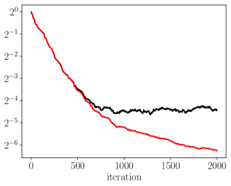
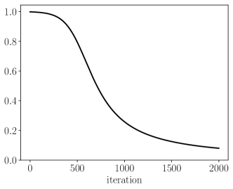
Figure 1. Left: relative error when using optimal learning rate $\alpha_{k}$ (red) and naive learning rate $\alpha_{k}=1$ (black). Right: plot of optimal learning rate $\alpha_{k}$. See Example 1.1 for details.

1.2. Background

The Kaczmarz algorithm dates back to the 1937 paper by Kaczmarz [13] who considered the iteration (2) for the case $\alpha_{k}=1$. The algorithm was subsequently studied by many authors; in particular, in 1967, Whitney and Meany [36] established a convergence result for the relaxed Kaczmarz algorithm: if $Ax=b$ is a consistent linear system, $i_{k}=k\mod m$, and $\alpha_{k}=\mu$ for fixed $0<\mu<2$, then (2) converges to $x$, see [36]. In 1970 the Kaczmarz algorithm was rediscovered under the name Algebraic Reconstruction Technique (ART) by Gordon, Bender, and Herman [7] who were interested in applications to computational tomography (including applications to three-dimensional electron microscopy); such applications typically use the relaxed Kaczmarz algorithm with learning rate $0<\alpha_{k}\leq 1$, see [12]. Methods and heuristics for setting the learning rate $\alpha_{k}$ have been considered by several authors, see the 1981 book by Censor [3]; also see [2, 9, 10].

More recently, in 2009, Strohmer and Vershynin [32] established the first proof of a convergence rate for a Kaczmarz algorithm that applies to general matrices; in particular, given a consistent linear system $Ax=b$, they consider the iteration (2) with $\alpha_{k}=1$. Under the assumption that the row index $i_{k}$ at iteration $k$ is chosen randomly with probability proportional to $\|a_{i_{k}}\|^{2}$ they prove that

$$\mathbb{E}\|x_{k}-x\|^{2}\leq(1-\eta)^{k}\|x-x_{0}\|^{2},$$ (3)

where $\eta:=\kappa(A)^{-2}$ and $\mathbb{E}$ is the expected value operator; here, $\kappa(A)$ is a condition number for the matrix $A$ defined by $\kappa(A):=\|A\|_{F}\|A^{-1}\|$, where $A^{-1}$ is the left inverse of $A$, $\|A^{-1}\|$ is the operator norm of $A^{-1}$, and $\|A\|_{F}$ is the Frobenius norm of $A$. We remark that the convergence rate in (3) is referred to as exponential convergence in [32], while in the field of numerical analysis (where it is typical to think about error on a logarithmic scale) it is referred to as linear convergence.

The result of [32] was subsequently extended by Needell [22] who considered the case of a noisy linear system: instead of having access to the right hand side of the consistent linear system $Ax=b$, we are given $\tilde{b}=b+\gamma$, where the entries of $\gamma$ satisfy $|\gamma_{i}|\leq\delta\|a_{i}\|$ but are otherwise arbitrary. Under these assumptions [22] proves that the iteration (2) with $\alpha_{k}=1$ satisfies

$$\mathbb{E}\|x_{k}-x\|^{2}\leq(1-\eta)^{k}\|x-x_{0}\|^{2}+\frac{\delta^{2}}{\eta},$$ (4)

that is, we converge in expectation until we reach some ball of radius $\delta/\sqrt{\eta}$ around the solution and then no more. Recall that $A^{-1}$ is the left inverse of $A$, and observe that

$$\|x-A^{-1}(b+\gamma)\|=\|A^{-1}\gamma\|\leq\|A^{-1}\|\|\gamma\|\leq\delta\|A^{-1}\|\|A\|_{F}=\frac{\delta}{\sqrt{\eta}}.$$ (5)

Moreover, if $\gamma$ is a scalar multiple of the left singular vector of $A$ associated with the smallest singular value, and $|\gamma_{i}|=\delta\|a_{i}\|$, then (5) holds with equality (such examples are easy to manufacture). Thus, (4) is optimal when $\gamma$ is arbitrary. In this paper, we consider the case where $\tilde{b}=b+\varepsilon$, where $\varepsilon$ has independent mean zero random entries: our main result shows that in this case, we break through the convergence horizon of (4) by using an optimized learning rate and many equations with independent noise, see Theorem 1.1 for a precise statement.

Remark 1.1 (Breaking through convergence horizon).

To be clear, when we say that our method breaks through the convergence horizon of (4), we mean that we are able to achieve expected error $\mathbb{E}\|x_{k}-x\|^{2}$ less than $\delta^{2}/\eta$. We achieve this by considering the model (2) where equations have independent noise and by using an optimal learning rate. Our main result establishes a bound on the expected error that decreases to zero as the number of available equations increases to infinity, which is the case in applications involving streaming, such as computational tomography. Note that under the model (2), determining the solution exactly requires an infinite number of equations; indeed, this is clearly the case even if the system of equations only has a single unknown. When a finite number of equations are available, we derive a precise bound on the expected error as a function of the number of iterations; Figure 1 demonstrates how the optimal learning rate improves the error compared to the standard Kaczmarz algorithm in a finite number of iterations.

1.3. Related work

Modifications and extensions of the randomized Kaczmarz algorithm have been considered by many authors, see [1, 5, 8, 15, 17, 19, 20, 23, 25, 29, 31, 33, 40]. We note that Cai, Zhao, and Tang [1] previously considered a relaxed Kaczmarz algorithm, but their analysis focuses on the case of a consistent linear system. More recently, Haddock, Needell, Rebrova, and Swartworth [8] considered the case of a consistent linear system corrupted by sparse noise; their main result proves convergence for a class of matrices by using an adaptive learning rate, which roughly speaking, attempts to avoid projecting onto corrupted equations. The result was subsequently generalized by Steinerberger [31]. Our results are complementary to the results of [8, 31]: we allow for corruption of all elements of $b$, but assume that corruptions are independent symmetric random variables; we show that, by using an optimal learning rate schedule, we can recover the solution to any accuracy if we have access to a sufficient number of equations with independent noise.

The randomized Kaczmarz algorithm of [32] can also be viewed as an instance of other machine learning methods. In particular, it can be viewed as an instance of coordinate descent, see [37], or as an instance of stochastic gradient descent, see [21], or an instance of the stochastic Newton method, see [4, 28]. Part of our motivation for studying learning rate schedules for the randomized Kaczmarz algorithm is that the randomized Kaczmarz algorithm provides a simple model where we can start to develop a complete theoretical understanding of the precise benefits of learning rates. The learning rate is of essential importance in machine learning; in particular, in deep learning: “The learning rate is perhaps the most important hyperparameter…. the effective capacity of the model is highest when the learning rate is correct for the optimization problem”, [6, pp. 429].

In this paper, we derive a scheduled learning rate (depending on two hyperparameters) for a randomized Kaczmarz algorithm, which optimizes a bound on the expected error, and prove an associated convergence result. Here, the word scheduled refers to the fact that the learning rate is determined a priori as a function of the iteration number and possibly hyperparameters (that is, the rate is non-adaptive). See [26, 38] for some general results about learning rate schedules.

1.4. Summary of main contributions

Given a consistent linear system of equations $Ax=b$, we study the problem of recovering the solution $x$ from $A$ and a corrupted right hand side $\tilde{b}$, where $\tilde{b}=b+\varepsilon$, and $\varepsilon$ has independent mean zero entries with bounded variance. We show the following:

• In contrast to the case of a consistent linear system (or a system with adversarial noise) changing the learning rate $\alpha_{k}$ is advantageous.

• We derive a scheduled learning rate that optimizes a bound on the expected error.

• In contrast to previous works related to the randomized Kaczmarz algorithm that exhibit exponential convergence, our optimized error bound involves the reciprocal of the Lambert-$W$ function of an exponential.

• In the limit as the number of iterations $k$ tends to infinity, the optimal learning rate $\alpha_{k}$ converges to time-based decay $1/(1+\eta k)$, which is a classic learning rate schedule.

• Our analysis has the potential to be combined with modifications of the randomized Kaczmarz algorithm to address other related problems, such as block-Kaczmarz methods or using the model (1) and (2) to study adaptive learning rates.

1.5. Main result

Let $A$ be an $m\times n$ matrix, $Ax=b$ be a consistent linear system of equations, and $a_{i}$ denote the $i$-th row of $A$. Suppose that $\tilde{b}$ is defined by

$$\tilde{b}=b+\varepsilon,$$

where $\varepsilon=(\varepsilon_{1},\ldots,\varepsilon_{m})$ are independent random variables such that $\varepsilon_{i}$ has mean $0$ and variance $\sigma^{2}\|a_{i}\|^{2}$. This assumption about the variance can be interpreted as assuming that the data has a common signal-to-noise ratio. Given $x_{0}$, define

$$x_{k+1}=x_{k}+\alpha_{k}\frac{\tilde{b}_{i_{k}}-\langle a_{i_{k}},x_{k}\rangle}{\|a_{i_{k}}\|^{2}}a_{i_{k}},$$ (6)

where $\alpha_{k}$ denotes the learning rate parameter; assume that $i_{k}$ is chosen from $\{1,\ldots,m\}\setminus\{i_{0},\ldots,i_{k-1}\}$ with probability proportional to $\|a_{i_{k}}\|^{2}$. Let $A_{k}$ denote the $(m-k)\times n$ matrix formed by deleting rows $\{i_{0},\ldots,i_{k-1}\}$ from $A$.

Theorem 1.1.

In addition to the assumptions stated in §1.5 above, assume that

$$\kappa(A_{k})^{-2}\geq\eta,\quad\text{for}\quad k\leq N{-1},$$ (7)

for some $N\leq m$. Given $\eta$ and $\|x-x_{0}\|^{2}/\sigma^{2}$ set, $\beta_{0}:=\|x-x_{0}\|^{2}/\sigma^{2}$ and define $\alpha_{k}$ recursively by

$$\alpha_{k}=\frac{\eta\beta_{k}}{\eta\beta_{k}+1},\quad\text{and}\quad\beta_{k+1}=\beta_{k}\left(1-\eta\alpha_{k}\right),\quad\text{for}\quad k=0,1,\ldots.$$ (8)

If $x_{k}$ is defined iteratively by (6), then

$$\mathbb{E}\|x_{k}-x\|^{2}\leq\sigma^{2}\beta_{k}\leq f(k),\quad\text{for}\quad k\leq N,$$ (9)

where

$$f(k):=\frac{\sigma^{2}}{\eta W(ce^{\eta k}{)}},\quad\text{for}\quad c:=\frac{\sigma^{2}}{\eta\|x-x_{0}\|^{2}}\exp\left(\frac{\sigma^{2}}{\eta\|x-x_{0}\|^{2}}\right),$$ (10)

where $W$ denotes the Lambert-$W$ function (the inverse of the function $x\mapsto xe^{x}$).

The proof of Theorem 1.1 is given in §2. In the following, we illustrate Theorem 1.1 with a mix of remarks, examples, and corollaries.

Remark 1.2 (Interpreting Theorem 1.1).

We summarize a few key observations that aid in interpreting Theorem 1.1:

1. Asymptotic behavior of $f(k)$: in the limit as the noise goes to zero

   $$f(k)\sim e^{-\eta k}\|x-x_{0}\|^{2},\quad\text{as}\quad\sigma\rightarrow 0,$$ (11)

   and in the limit as the number of iterations go to infinity

   $$f(k)\sim\frac{\sigma^{2}}{\eta^{2}k},\quad\text{as}\quad k\rightarrow\infty,$$ (12)

   see Corollary 1.1 and 1.2, respectively, for more precise statements. In particular, this implies that $\mathbb{E}\|x-x_{k}\|^{2}$ tends to $0$ as $k\rightarrow\infty$ (letting $k$ tend to infinity requires letting $N$ tend to infinity, which requires an increasing number of equations $m$ with independent noise, see bullet point ((iii)) below).

2. Informally speaking, the assumption (7) says that the submatrix of the remaining rows remains well-conditioned as we run the algorithm. If $A$ is an $m\times n$ random matrix with i.i.d. rows, then (7) can be replaced by a condition on the distribution of $A$, which is independent of the iteration number $k$. In this case, the result (9) holds for all $k\leq m$, see Corollary 1.3.

3. We emphasize that $i_{k}$ is chosen without replacement, see §1.5, so the maximum number of iterations is at most the number of rows $m$. In practice, the algorithm can be run with restarts: after a complete pass over the data we use the final iterate to redefine $x_{0}$, and restart the algorithm (potentially using different hyperparameters to define the learning rate). In the context of machine learning, the statement of Theorem 1.1 applies to one epoch, see §4.

4. The error bound $f(k)$ is sharp in some cases; in these cases the learning rate is optimal, see Corollary 1.4. We demonstrate this corollary numerically in Figure 2.

Example 1.1 (Numerical illustration of Theorem 1.1).

Let $A$ be an $m\times n$ matrix with $s$ nonzero entries in each row. Assume these nonzero entries are independent vectors drawn uniformly at random from the unit sphere: $S^{s-1}=\{v\in\mathbb{R}^{s}:\|v\|=1\}$. Let $x$ be an $n$-dimensional vector with independent standard normal entries, and set $b:=Ax$. Let $\tilde{b}=b+\varepsilon$, where $\varepsilon$ is an $m$-dimensional vector with independent mean $0$, variance $\sigma^{2}$ normal entries. We run the relaxed Kaczmarz algorithm (2) using the learning rate (8) of Theorem 1.1. In particular, we set

$$m=2000,\quad n=100,\quad s=10,\quad\sigma=.05,\quad\text{and}\quad x_{0}=\vec{0}.$$

Using the estimates $\|x-x_{0}\|^{2}=n$ and $\eta=1/100$ we define $\alpha_{k}$ by (8). This choice of $\eta$ is justified by Corollary 1.4 below in combination with the fact that the rows of $A$ are isotropic when scaled by $\sqrt{n}$, see [35, §3.2.3, §3.3.1]. We plot the numerical relative error $\|x-x_{k}\|/\|x\|$ together with the bound on the expected relative error $\sqrt{f(k)}/\|x\|$ in Figure 2. Furthermore, to provide intuition about how $f(k)$ varies with $\sigma$, we plot $\sqrt{f(k)}/\|x\|$ for various values of $\sigma$ in Figure 2, keeping other parameters fixed.

At first, when $\|x-x_{k}\|^{2}\gg\sigma^{2}$, (roughly iterations 1 to 500, see Figure 1) the error decreases linearly in the logarithmic scale of the figure illustrating the asymptotic rate (11). For large $k$, when $\|x-x_{k}\|^{2}\ll\sigma^{2}$ (after roughly 1000 iterations, see Figure 1) the error decreases like $1/\ln k$ in the logarithmic scale of the figure, illustrating the asymptotic rate (12).

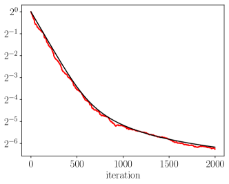
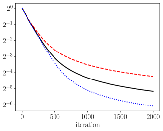
Figure 2. Left: relative error $\|x-x_{k}\|/\|x\|$ (red), and function $\sqrt{f(k)}/\|x\|$ (black). Right: how the function $\sqrt{f(k)}/\|x\|$ changes when $\sigma=.05$ (dotted blue), $\sigma=.1$ (solid black), and $\sigma=.2$ (dashed red). See Example 1.1 for details.

Example 1.2 (Continuous version of learning rate $\alpha_{k}$).

The learning rate $\alpha_{k}$ defined in (8) optimizes the error bound of Theorem 1.1, see §2.4. The scheduled learning rate $\alpha_{k}$ depends on two parameters (assuming $x_{0}=\vec{0}$):

• the signal-to-noise ratio $\|x\|^{2}/\sigma^{2}$, and

• the condition number parameter $\eta$.

The result of Theorem 1.1 states that the function $f(k)$ defined in (10) is an upper bound for $\beta_{k}\sigma^{2}$. From the proof of Theorem 1.1 it will be clear that this upper bound is a good approximation when $\eta$ is small, see §2.5. In this case, it is illuminating to consider a continuous version of the optimal scheduled learning rate of Theorem 1.1. In particular, we define

$$\alpha(t)=\frac{\eta f(t)}{\eta f(t)+\sigma^{2}},$$ (13)

where $f(t)$ is defined by (10). We plot the function $\alpha(t)$ for three different levels of noise: $\sigma=.01$, $\sigma=.1$, and $\sigma=1$, while keeping the other parameters fixed (and set by the values in Example 1.1), see Figure 3.

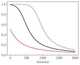
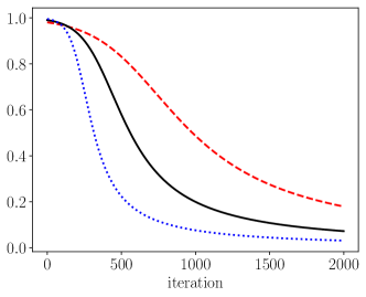
Figure 3. Left: $\alpha(t)$ for $\sigma=.01$ (dotted blue), $\sigma=.1$ (solid black), and $\sigma=1$ (dashed red). Right: $\alpha(t)$ for $\eta=.005$ (dashed red), $\eta=.01$ (solid black),and $\eta=.02$ (dotted blue).

We also plot the function $\alpha(t)$ for three different values of the condition number parameter: for $\eta=.005$, $\eta=.01$ and $\eta=.02$, while keeping the other parameters fixed (and set by the values in Example 1.1), see Figure 3.

Remark 1.3 (Asymptotics of $\alpha(t)$).

The continuous version of the learning rate (13) has two distinct asymptotic regimes similar to Remark 1.2 ((i)). In particular, in the limit as the noise goes to zero we have

$$\alpha(t)\sim 1,\quad\text{as}\quad\sigma\rightarrow 0,$$ (14)

and in the limit as the number of iterations goes to infinity we have

$${\alpha}(t)\sim\frac{1}{1+\eta{t}},\quad\text{as}\quad{t}\rightarrow\infty.$$ (15)

The regimes (14) and (15) are illustrated by the blue dotted line in the left and right plots of Figure 3, respectively. We note that (15) corresponds to time-based decay, which is a popular learning rate in practice, see the learning rate schedules of [34].

Example 1.3 (Optimal learning rate versus time-based decay).

We compare the optimal learning rate $\alpha_{k}$ to the time-based decay learning rate $1/(1+\eta k)$, which is the large iteration limit of the optimal learning rate, see (15). We run the Kaczmarz algorithm (2) with these learning rates for the system described in Example 1.1, see Figure 4.

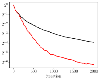
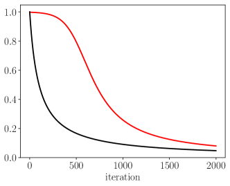
Figure 4. Left: relative error when using optimal learning rate $\alpha_{k}$ (red) and time-based decay $1/(1+\eta k)$ (black). Right: plot of optimal learning rate $\alpha_{k}$ (red), and time-based decay (black)

The fact that time-based decay $1/(1+\eta k)$ is the large iteration limit of the optimal learning rate $\alpha_{k}$ is reflected in the fact that eventually (after $1500$ iterations) both errors appear to decrease at similar rates. However, initially the optimal learning rate decreases the error much faster and a gap between the two relative errors appears (and this gap will remain). Informally speaking, the reason that using an ‘S’-shaped learning rate is optimal is that initially, when the error is larger than the noise, it is advantageous to keep the learning rate close to $1$ (to make rapid initial progress), and to only decrease the learning rate once the error is smaller than the noise. It is instructive to compare these results to Figure 1, where we plot the errors of the optimal learning rate to the constant learning rate $1$, which is the small noise limit of the optimal learning rate, see (14). Observe that in Figure 1, the errors initially decrease at the same rate, but eventually the error associated with the constant learning rate stagnates. Informally speaking, the optimal learning rate can be viewed as an optimal transition between the constant learning rate $1$ and time-based decay $1/(1+\eta k)$.

Example 1.4 (Estimating hyperparameters).

As noted in Example 1.2, the scheduled learning rate $\alpha_{k}$ defined in Theorem 1.1 depends on two hyperparameters the signal-to-noise ratio $\|x\|^{2}/\sigma^{2}$, and the condition number parameter $\eta$. In order to use this learning rate in practice, it is necessary to estimate these parameters. Indeed, commonly used Learning rate schedules such as the constant learning rate, time-based decay, step-based decay, and exponential decay depend on one or more parameters [34], and the problem of tuning these hyperparameters is important in practice [6]. The fact that the hyperparameters of the of the learning rate schedule $\alpha_{k}$ of Theorem 1.1 have natural interpretations as the signal-to-noise-ratio and condition number parameter, respectively, provides addition intuition towards tuning these parameters.

We next show a heuristic to estimate the parameters $\eta$ and $\|x\|^{2}/\sigma^{2}$ from one additional run of the randomized Kaczmarz method. Let $x_{0},\ldots,x_{N}$ denote the iterates resulting from running the randomized Kaczmarz algorithm (2) with constant learning rate $1$ for $N$ iterations. If we assume the initial error is above the noise level, and assume that eventually the error stagnates because of the noise, then we expect that, initially, $\|x_{j+1}-x\|^{2}\approx(1-\eta)\|x_{j}-x\|^{2}$, see (19), and eventually $\|x_{j}-x\|^{2}\approx\sigma^{2}/\eta$, see (4). Using these estimates and the approximation $\|x_{N}\|^{2}\approx\|x\|^{2}$ yields the heuristic estimates for $\eta$ and $\beta_{0}=\|x\|^{2}/\sigma^{2}$

$$\tilde{\eta}:=1-\frac{1}{N_{0}}\sum_{j=1}^{N_{0}}\frac{\|x_{j}-x_{N}\|^{2}}{\|x_{j-1}-x_{N}\|^{2}},\quad\text{and}\quad\tilde{\beta}_{0}^{-1}:=\tilde{\eta}\frac{1}{N_{1}}\sum_{j=N-N_{1}}^{N-1}\frac{\|x_{N}-x_{j}\|^{2}}{\|x_{N}\|^{2}},$$ (16)

for some integers $N_{0}$ and $N_{1}$. Suppose that the system described in Example 1.1 is given, but the parameter condition number parameter $\eta$ and the signal-to-noise ratio $\|x\|^{2}/\sigma^{2}$ are unknown. In Figure 5, we show the result of running the Kaczmarz method with the estimated learning rate $\tilde{\alpha}_{k}$ obtained from the parameters estimated by (16), using $N_{0}=100$, $N_{1}=100$ and $N=2000$.

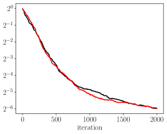
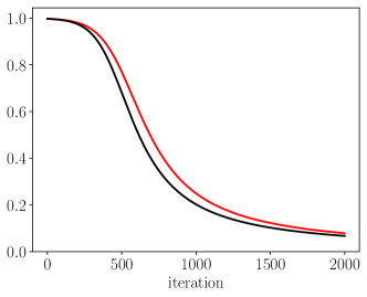
Figure 5. Left: relative error when using optimal $\alpha_{k}$ (red) and estimated $\tilde{\alpha}_{k}$ (black) learning rate Right: plot of optimal $\alpha_{k}$ (red) and estimated $\tilde{\alpha}_{k}$ (black) learning rate.

Remark 1.4 (Normalizing rows).

Practically speaking, before the algorithm starts, the rows of the linear system can simply be normalized so that they have the same norm. We note that this can be considered as a form of preconditioning, which will change the condition number of the matrix. This row normalization simplifies the application of the randomized Kaczmarz method and can be performed as the rows are sampled in a streaming setting, as assumed in for example [8].

Example 1.5 (Computational tomography example).

We lastly include a real-world example of a tomography simulation of a system of equations $Ax=b$. The matrix $A$ has dimensions $4500\times 225$ and corresponds to absorption along a random line through a $15\times 15$ grid. The matrix $A$ and the vector $x$ were generated from the Matlab Regularization Toolbox by P.C. Hansen [11] and $x$ was normalized to have unit norm. The right hand side $b$ of the consistent system generated by the simulation is corrupted by adding noise according to (1).

The numerical example combines the considerations in the preceding remarks and examples: we normalize the rows of $A$ (see Remark 1.4), the hyperparameters $\eta$ and $\|x\|^{2}/\sigma^{2}$ are estimated (see Remark 1.4) and multiple epochs are used. Note that while Theorem 1.1 only applies to one epoch (see Remark 1.2(iii)) since we require equations with independent noise, practically speaking the result may continue to hold over multiple epochs as long as (24) in the Proof of Theorem 1.1 approximately holds.

The results are shown in Figure 6 for two different values of the noise. Note the similarities between Figure 6 and Figure 1, indicating that the framework of the article applies well beyond the conditions of Theorem 1.1.

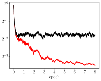
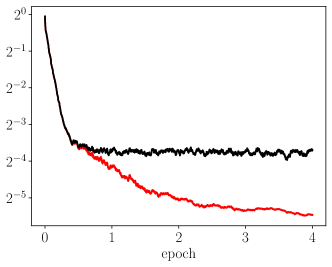
Figure 6. Relative error of constant learning rate when using constant learning rate $1$ (black) and estimated learning rate (red) for $\sigma=0.02$ (left). and $\sigma=0.005$ (right).

1.6. Corollaries of the main result

The following corollaries provide more intuition about the error bound function $f(k)$, and cases when the error bound of Theorem 1.1 is sharp. First, we consider the case where the variance of the noise $\sigma^{2}$ is small, and the other parameters are fixed; in this case we recover the convergence rate of the standard randomized Kaczmarz algorithm with $\eta=\kappa(A)^{-2}$.

Corollary 1.1 (Limit as $\sigma\rightarrow 0$).

We have

$$f(k)=e^{-\eta k}\|x-x_{0}\|^{2}\left(1+\mathcal{O}\left(\frac{\sigma^{2}}{\|x-x_{0}\|^{2}}\right)\right),\quad\text{as}\quad\sigma\rightarrow 0,$$

where the constant in the big-$\mathcal{O}$ notation depends on $\eta$ and $k$.

The proof of Corollary 1.1 is given in §3.1. Next, we consider the convergence rate as the number of iterations goes to infinity and the other parameters are fixed.

Corollary 1.2 (Limit as $k\rightarrow\infty$).

We have

$$f(k)=\frac{\sigma^{2}}{\eta^{2}k}\left(1+\mathcal{O}\left(\frac{\ln k}{k}\right)\right),\quad\text{as}\quad k\rightarrow\infty,$$

where the constant in the big-$\mathcal{O}$ notation depends on $\eta$, $\|x-x_{0}\|^{2}$ and $\sigma^{2}$.

The proof of Corollary 1.2 is given in §3.2. Informally speaking, in combination with Theorem 1.1 and Jensen’s inequality, this corollary says that we should expect

$$\mathbb{E}\|x-x_{k}\|\lesssim\frac{\sigma}{\eta}\frac{1}{\sqrt{k}},$$

which agrees with the intuition (based on the central limit theorem) that using $k$ independent sources of noise should reduce the expected error by a factor of $1/\sqrt{k}$.

Corollary 1.3 (Matrices with i.i.d. rows).

Suppose that $A$ is an $m\times n$ random matrix with i.i.d. rows, and let $a_{0}$ be a random variable generated according to this distribution. If we run the algorithm (2) with $i_{k}=k$, and in place of the condition (7) assume that

$$\mathbb{E}\left|\left\langle z,\frac{{a_{0}}}{\|{a_{0}}\|}\right\rangle\right|^{2}\geq\eta\|z\|^{2},\quad\forall z\in\mathbb{R}^{n},$$ (17)

for some fixed value $\eta>0$, where the expectation is over the random variable $a_{0}$. Then the result (9) of Theorem 1.1 holds for $k\leq m$.

The proof of Corollary 1.3 is given in §3.3. The condition of Corollary 1.3 holds if, for example, the rows of $A$ are sampled uniformly at random from the unit sphere $S^{n-1}=\{x\in\mathbb{R}^{n}:\|x\|=1\}$. Indeed, in this case

$$\mathbb{E}\left|\left\langle z,a_{0}\right\rangle\right|^{2}\geq\frac{1}{n}\|z\|^{2},\quad\forall z\in\mathbb{R}^{n},$$

see [35, Lemma 3.2.3, §3.3.1]. The following corollary gives a condition under which the learning rate (8) is optimal. In particular, this corollary implies that the error bound and learning rate are optimal for the example of matrices whose rows are sampled uniformly at random from the unit sphere discussed above.

Corollary 1.4 (Case when error bound is sharp and learning rate is optimal).

Assume that

$$\mathbb{E}_{i_{0},\ldots,i_{k-1}}\left|\left\langle\frac{x_{k}-x,}{\|x-x_{k}\|},\frac{a_{i_{k}}}{\|a_{i_{k}}\|}\right\rangle\right|^{2}=\eta.$$ (18)

Then,

$$\mathbb{E}\|x-x_{k}\|^{2}=\sigma^{2}\beta_{k},$$

and the learning rate $\alpha_{k}$ defined by (8) is optimal in the sense that it minimizes the expected error $\mathbb{E}\|x-x_{k}\|^{2}$ over all possible choices of scheduled learning rates (learning rates that only depend on the iteration number $k$ and possibly hyperparameters). Moreover, if (17) holds with $\eta=1/n$, then it follows that (18) holds with equality and hence the learning rate is optimal.

The proof of Corollary 1.4 is given in §3.4. Informally speaking, the learning rate $\alpha_{k}$ defined by (8) is optimal whenever the bound $\beta_{k}\sigma^{2}$ in Theorem 1.1 is a good approximation of the expected error $\mathbb{E}\|x-x_{k}\|^{2}$, and there is reason to expect this is the case in practice, see the related results for consistent systems [32, §3, Theorem 3] and [30, Theorem 1]. For additional discussion about Theorem 1.1 and its corollaries see §4.

2. Proof of Theorem 1.1

The proof of Theorem 1.1 is divided into five steps:

• Step 1 (§2.1) We consider the relaxed Kaczmarz algorithm for the consistent linear system $Ax=b$ and prove a recursive formula for the expected error of the solution. This step uses the same proof strategy as [32].

• Step 2 (§2.2). We consider the effect of additive random noise. More precisely, we study how the additive noise changes the analysis of Step 1. The end result is additional terms involving conditional expectations of a geometric quantity $\eta_{k}$ and a noise quantity $\zeta_{k}$, with respect to the choices of rows $i_{0},\ldots,i_{k-1}$.

• Step 3 (§2.3). We estimate the conditional expectations of the geometric quantity $\eta_{k}$ and a noise quantity $\zeta_{k}$.

• Step 4 (§2.4). We optimize the learning rate $\alpha_{k}$ with respect to the error bound from the previous step. This results in a recurrence relation for the optimal learning rate.

• Step 5 (§2.5). We show that this optimized learning rate is related to a differential equation, which can be used to establish the upper bound $f(k)$ on the expected error.

2.1. Step 1: relaxed randomized Kaczmarz for consistent systems

We start by considering the consistent linear system $Ax=b$. Assume that $x_{0}$ is given and let

$$x_{k+1}:=x_{k}+\alpha_{k}\frac{b_{i_{k}}-\langle a_{i_{k}},x_{k}\rangle}{\|a_{i_{k}}\|^{2}}a_{i_{k}},$$

denote the iteration of the relaxed randomized Kaczmarz algorithm with learning rate $\alpha_{k}$ on the consistent linear system $Ax=b$, and let

$$y_{k+1}:=x_{k}+\frac{b_{i_{k}}-\langle a_{i_{k}},x_{k}\rangle}{\|a_{i_{k}}\|^{2}}a_{i_{k}},$$

be the projection of $x_{k}$ on the affine hyperplane defined by the $i_{k}$-th equation. The points $y_{k+1},x_{k+1}$, and $x_{k}$ lie on the line $\{x_{k}+ta_{i_{k}}:t\in\mathbb{R}\}$, which is perpendicular to the affine hyperplane $\{y\in\mathbb{R}^{n}:\langle a_{i_{k}},y\rangle=b_{i_{k}}\}$ that contains $x$ and $y_{k+1}$, see the illustration in Figure 7.

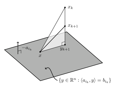
Figure 7. Illustration of the points $x,y_{k+1},x_{k+1}$, and $x_{k}$.

By the Pythagorean theorem, it follows that

$$\|x-x_{k+1}\|^{2}=\|x-x_{k}\|^{2}-\|y_{k+1}-x_{k}\|^{2}+\|y_{k+1}-x_{k+1}\|^{2},$$

and by definition of $y_{k+1}$ and $x_{k+1}$ we have

$$y_{k+1}-x_{k+1}=(1-\alpha_{k})(y_{k+1}-x_{k}),$$

see Figure 7. Thus

$$\|x-x_{k+1}\|^{2}=\|x-x_{k}\|^{2}-(2\alpha_{k}-\alpha_{k}^{2})\|y_{k+1}-x_{k}\|^{2}.$$

Factoring out $\|x-x_{k}\|^{2}$ from the right hand side gives

$$\|x-x_{k+1}\|^{2}=\left(1-(2\alpha_{k}-\alpha_{k}^{2})\frac{\|y_{k+1}-x_{k}\|^{2}}{\|x-x_{k}\|^{2}}\right)\|x-x_{k}\|^{2}.$$

Since $\|y_{k+1}-x_{k}\|=|\langle x_{k}-x,a_{i_{k}}/\|a_{i_{k}}\|\rangle|$, it follows that

$$\|x_{k+1}-x\|^{2}=\left(1-(2\alpha_{k}-\alpha_{k}^{2})\left|\left\langle\frac{x_{k}-x}{\|x_{k}-x\|},\frac{a_{i_{k}}}{\|a_{i_{k}}\|}\right\rangle\right|^{2}\right)\|x_{k}-x\|^{2}.$$

Taking the expectation conditional on $\{i_{0},\ldots,i_{k-1}\}$ gives

$$\mathbb{E}_{i_{0},\ldots,i_{k-1}}\|x_{k+1}-x\|^{2}=\left(1-(2\alpha_{k}-\alpha_{k}^{2})\eta_{k}\right)\|x_{k}-x\|^{2},$$ (19)

where

$$\eta_{k}:=\mathbb{E}_{i_{0},\ldots,i_{k-1}}\left|\left\langle\frac{x_{k}-x}{\|x_{k}-x\|},\frac{a_{i_{k}}}{\|a_{i_{k}}\|}\right\rangle\right|^{2}.$$

We delay discussion of conditional expectation until Step 3 (§2.3).

Remark 2.1 (Optimal learning rate for consistent linear systems).

Observe that

$$(1-\eta_{k})\|x_{k}-x\|^{2}\leq\left(1-(2\alpha_{k}-\alpha_{k}^{2})\eta_{k}\right)\|x_{k}-x\|^{2},$$

with equality only when $\alpha_{k}=1$. It follows that, for consistent linear systems of equations, the optimal way to define the learning rate is to set $\alpha_{k}=1$ for all $k=0,1,2,\ldots$. In the following, we show that, under our noise model, defining $\alpha_{k}$ as a specific decreasing function of $k$ is advantageous.

2.2. Step 2: relaxed randomized Kaczmarz for systems with noise

In this section, we redefine $x_{k}$ and $y_{k}$ for the case where the right hand side of the consistent linear system $Ax=b$ is corrupted by additive random noise: $\tilde{b}=b+\varepsilon$. Let

$$x_{k+1}:=x_{k}+\alpha_{k}\frac{\tilde{b}_{i_{k}}-\langle a_{i_{k}},x_{k}\rangle}{\|a_{i_{k}}\|^{2}}a_{i_{k}}=x_{k}+\alpha_{k}\frac{b_{i_{k}}+\varepsilon_{i_{k}}-\langle a_{i_{k}},x_{k}\rangle}{\|a_{i_{k}}\|^{2}}a_{i_{k}},$$

be the iteration of the relaxed randomized Kaczmarz algorithm using $\tilde{b}$, and

$$y_{k+1}:=x_{k}+\frac{b_{i_{k}}-\langle a_{i_{k}},x_{k}\rangle}{\|a_{i_{k}}\|^{2}}a_{i_{k}},$$

be the projection of $x_{k}$ on the affine hyperplane defined by the uncorrupted $i_{k}$-th equation. Note that both $x_{k+1}$ and $y_{k+1}$ differ from the previous section: $x_{k+1}$ is corrupted by the noise term $\varepsilon_{i_{k}}$ and $y_{k+1}$ is the projection of the previously corrupted iterate $x_{k}$ onto the hyperplane defined by the uncorrupted equation. However, the following expansion still holds:

$$\|x-x_{k+1}\|^{2}=\|x-x_{k}\|^{2}-\|y_{k+1}-x_{k}\|^{2}+\|y_{k+1}-x_{k+1}\|^{2}.$$ (20)

Indeed, $x_{k+1},y_{k+1},$ and $x_{k}$ are still contained on the line $\{x_{k}+ta_{i_{k}}:t\in\mathbb{R}\}$, which is perpendicular to the affine hyperplane $\{y\in\mathbb{R}^{n}:\langle a_{i_{k}},y\rangle=b_{i_{k}}\}$ that contains $x$ and $y_{k+1}$, see Figure 7. By the definition of $y_{k+1}$ and $x_{k+1}$ we have

$$\|y_{k+1}-x_{k+1}\|^{2}=\left\|(1-\alpha_{k})(y_{k+1}-x_{k})-\alpha_{k}\frac{\varepsilon_{i_{k}}}{\|a_{i_{k}}\|}\frac{a_{i_{k}}}{\|a_{i_{k}}\|}\right\|^{2}.$$

Expanding the right hand side gives

$$\|y_{k+1}-x_{k+1}\|^{2}=(1-\alpha_{k})^{2}\|y_{k+1}-x_{k}\|^{2}+Z_{k},$$ (21)

where

$$Z_{k}:=-2\alpha_{k}(1-\alpha_{k})\frac{\varepsilon_{i_{k}}}{\|a_{i_{k}}\|}\left\langle y_{k+1}-x_{k},\frac{a_{i_{k}}}{\|a_{i_{k}}\|}\right\rangle+\alpha_{k}^{2}\frac{\varepsilon_{i_{k}}^{2}}{\|a_{i_{k}}\|^{2}}.$$

By using the fact that

$$\left\langle y_{k+1}-x_{k},\frac{a_{i_{k}}}{\|a_{i_{k}}\|}\right\rangle=\frac{b_{i_{k}}-\langle a_{i_{k}},x_{k}\rangle}{\|a_{i_{k}}\|},$$

we can rewrite $Z_{k}$ as

$$Z_{k}=-2\alpha_{k}(1-\alpha_{k})\frac{\varepsilon_{i_{k}}}{\|a_{i_{k}}\|}\frac{b_{i_{k}}-\langle a_{i_{k}},x_{k}\rangle}{\|a_{i_{k}}\|}+\alpha_{k}^{2}\frac{\varepsilon_{i_{k}}^{2}}{\|a_{i_{k}}\|^{2}}.$$

Combining (20) and (21) gives

$$\|x-x_{k+1}\|^{2}=\|x-x_{k}\|^{2}-(2\alpha_{k}-\alpha_{k}^{2})\|y_{k+1}-x_{k}\|^{2}+Z_{k}.$$

As in the analysis of the consistent linear system in Step 1 (§2.1) above, we factor out $\|x-x_{k}\|^{2}$, use the fact that $\|y_{k+1}-x_{k}\|=\langle x_{k}-x,a_{i_{k}}/\|a_{i_{k}}\|\rangle$, and take the expectation conditional on $\{i_{0},\ldots,i_{k-1}\}$ to conclude that

$$\mathbb{E}_{i_{0},\ldots,i_{k-1}}\|x_{k+1}-x\|^{2}=\big{(}1-(2\alpha_{k}-\alpha_{k}^{2})\eta_{k}\big{)}\|x_{k}-x\|^{2}+\zeta_{k},$$ (22)

where

$$\eta_{k}:=\mathbb{E}_{i_{0},\ldots,i_{k-1}}\left|\left\langle\frac{x_{k}-x}{\|x_{k}-x\|},\frac{a_{i_{k}}}{\|a_{i_{k}}\|}\right\rangle\right|^{2},\quad\text{and}\quad\zeta_{k}=\mathbb{E}_{i_{0},\ldots,i_{k-1}}Z_{k}.$$

In the following section, we discuss the terms $\zeta_{k}$ and $\eta_{k}$.

2.3. Step 3: estimating conditional expectations

In this section, we discuss estimating the conditional expectations $\eta_{k}$ and $\zeta_{k}$. First, we discuss $\zeta_{k}$, which has two terms (a linear term and quadratic term with respect to $\varepsilon_{i_{k}}$). In particular, we have

$$\zeta_{k}=-2\alpha_{k}(1-\alpha_{k})\mathbb{E}_{i_{0},\ldots,i_{k-1}}\frac{\varepsilon_{i_{k}}}{\|a_{i_{k}}\|}\frac{b_{i_{k}}-\langle a_{i_{k}},x_{k}\rangle}{\|a_{i_{k}}\|}+\alpha_{k}^{2}\mathbb{E}_{i_{0},\ldots,i_{k-1}}\frac{\varepsilon_{i_{k}}^{2}}{\|a_{i_{k}}\|^{2}}.$$ (23)

Recall that $\varepsilon_{1},\ldots,\varepsilon_{m}$ are independent random variables such that $\varepsilon_{i_{k}}$ has mean zero and variance $\sigma^{2}\|a_{i_{k}}\|^{2}$. Since we assume that $i_{k}$ is chosen from $\{1,\ldots,m\}\setminus\{i_{0},\ldots,i_{k-1}\}$ (that is, they are drawn without replacement) with probability proportional to $\|a_{i_{k}}\|^{2}$, see §1.5, it follows that $\varepsilon_{i_{k}}/\|a_{i_{k}}\|$ is independent from $(b_{i_{k}}-\langle a_{i_{k}},x_{k}\rangle)/\|a_{i_{k}}\|$. Hence

$$\zeta_{k}=\alpha_{k}^{2}\sigma^{2}.$$ (24)

We remark that if $i_{k}$ was chosen uniformly at random from $\{1,\ldots,m\}$ and we had previously selected equation $i_{k}$, say, during iteration $j$ for $j<k$, then the error in the $i_{k}$-th equation $b_{i_{k}}-\langle a_{i_{k}},x_{k}\rangle$ may depend (or even be determined) by $\varepsilon_{i_{k}}$; thus the assumption that rows are drawn without replacement is necessary for this term to vanish. We use the same estimate for $\eta_{k}$ as in [32]. In particular, by [32, eq. 7] we have

$$\eta_{k}=\mathbb{E}_{i_{0},\ldots,i_{k-1}}\left|\left\langle\frac{x_{k}-x,}{\|x-x_{k}\|},\frac{a_{i_{k}}}{\|a_{i_{k}}\|}\right\rangle\right|^{2}\geq\kappa(A_{k})^{-2}\geq\eta,$$ (25)

where the final inequality follows by assumption (7) in the statement of Theorem 1.1.

Remark 2.2 (Comparison to case $\alpha_{k}=1$).

Note that when $\alpha_{k}=1$, the linear term of (23) satisfies

$$-2\alpha_{k}(1-\alpha_{k})\mathbb{E}_{i_{0},\ldots,i_{k-1}}\frac{\varepsilon_{i_{k}}}{\|a_{i_{k}}\|}\frac{b_{i_{k}}-\langle a_{i_{k}},x_{k}\rangle}{\|a_{i_{k}}\|}=0$$

because $(1-\alpha_{k})=0$, which geometrically is the result of an orthogonality relation, which holds regardless of the structure of the noise. Here we consider the case $\alpha_{k}\not=1$, and the linear term vanishes due to the assumption that $\varepsilon_{i}$ are independent mean zero random variables.

2.4. Step 4: optimal learning rate with respect to upper bound

In this section we derive the optimal learning rate $\alpha_{k}$ with respect to an upper bound on the expected error. In Remark 2.1, we already considered the case $\sigma=0$, and found that the optimal learning rate is to set $\alpha_{k}=1$ for all $k=0,1,\ldots$ regardless of the other parameters. Thus, in this section we assume that $\sigma>0$. By (22), (24), and (25) we have

$$\mathbb{E}_{i_{0},\ldots,i_{k-1}}\|x_{k+1}-x\|^{2}\leq\Big{(}1-(2\alpha_{k}-\alpha_{k}^{2})\eta\Big{)}\|x_{k}-x\|^{2}+\alpha_{k}^{2}\sigma^{2}.$$ (26)

Iterating this estimate and taking a full expectation gives

$$\mathbb{E}\|x_{k+1}-x\|^{2}\leq g(k,\alpha)\sigma^{2},$$

for

$$g(k,\alpha):=\prod_{j=0}^{k}\Big{(}1-(2\alpha_{j}-\alpha_{j}^{2})\eta\Big{)}\frac{\|x_{0}-x\|^{2}}{\sigma^{2}}+\sum_{j=0}^{k}\alpha_{j}^{2}\prod_{i=j+1}^{k}\Big{(}1-(2\alpha_{i}-\alpha_{i}^{2})\eta\Big{)},$$

where $\alpha=\{\alpha_{j}\}_{j=0}^{N}$ and we use the convention that empty products are equal to $1$. Note that since the sums and products defining $g(k,\alpha)$ range up to $k$, it follows that $g(k,\alpha)$ does not depend on $\alpha_{j}$ for $j\geq k+1$. This upper bound $g(k,\alpha)$ satisfies the recurrence relation

$$g(k,\alpha)=\Big{(}1-(2\alpha_{k}-\alpha_{k}^{2})\eta\Big{)}g(k-1,\alpha)+\alpha_{k}^{2},$$

where $g(k-1,\alpha)$ does not depend on $\alpha_{k}$. Setting the partial derivative $\partial_{\alpha_{k}}g$ of $g$ with respect to $\alpha_{k}$ equal to zero, and solving for $\alpha_{k}$ gives

$$\alpha_{k}=\frac{\eta g(k-1,\alpha)}{\eta g(k-1,\alpha)+1}.$$ (27)

Since $\partial^{2}_{\alpha_{k}}g(k,\alpha)=2\eta g(k-1,\alpha)+2\sigma^{2}>0$ the value of $\alpha_{k}$ defined by (27) does indeed minimize $g(k,\alpha)$ with respect to $\alpha_{k}$. It is straightforward to verify that this argument can be iterated to conclude that the values of $\alpha_{0},\alpha_{1},\ldots$ that minimize $g(k,\alpha)$ satisfy the recurrence relation:

$$\begin{split}\beta_{0}&:=\|x-x_{0}\|^{2}/\sigma^{2},\\ \alpha_{k}&=\frac{\eta\beta_{k}}{\eta\beta_{k}+1}\quad\text{and}\quad\beta_{k+1}=\Big{(}1-(2\alpha_{k}-\alpha_{k}^{2})\eta\Big{)}\beta_{k}+\alpha_{k}^{2},\end{split}$$ (28)

for $k=0,1,\ldots$. Note that we can simplify (28) by observing that

$$\begin{split}-(2\alpha_{k}-\alpha_{k}^{2})\eta\beta_{k}+\alpha_{k}^{2}&=\frac{-\left(2\eta\beta_{k}(\eta\beta_{k}+1)-\eta^{2}\beta_{k}^{2}\right)\eta\beta_{k}+\eta^{2}\beta_{k}^{2}}{(\eta\beta_{k}+1)^{2}}\\ &=\frac{-\eta^{2}\beta_{k}^{2}}{\eta\beta_{k}+1}=-\eta\beta_{k}\alpha_{k}.\end{split}$$

In summary, we can compute the optimal learning rate $\alpha_{k}$ with respect to the upper bound $g(k,\alpha)$ on the expected error $\mathbb{E}\|x-x_{k}\|^{2}$ as follows: if $\sigma^{2}=0$, then $\alpha_{k}=1$ for all $k$. Otherwise, we define

$$\begin{split}\beta_{0}&=\|x-x_{0}\|^{2}/\sigma^{2},\\ \alpha_{k}&=\frac{\eta\beta_{k}}{\eta\beta_{k}+1},\quad\text{and}\quad\beta_{k+1}=\beta_{k}(1-\eta\alpha_{k}),\end{split}$$ (29)

for $k=0,1,\ldots$. In the following section we study the connection between this recursive formula and a differential equation.

2.5. Step 5: relation to differential equation

In this section, we derive a closed form upper bound for $\beta_{k}$. It follows from (29) that

$$\frac{\eta\beta_{k+1}-\eta\beta_{k}}{\eta}=-\eta\beta_{k}\frac{\eta\beta_{k}}{\eta\beta_{k}+1}.$$

Making the substitution $u_{k}:=\eta\beta_{k}$ gives the finite difference equation

$$\frac{u_{k+1}-u_{k}}{\eta}=-\frac{u_{k}^{2}}{u_{k}+1},$$

which can be interpreted as one step of the forward Euler method (with step size $\eta$) for the ordinary differential equation

$$\dot{u}=-\frac{u^{2}}{u+1},$$ (30)

where $u=u(t)$ and $\dot{u}=du/dt$. It is straightforward to verify that the solution of this differential equation is

$$u(t)=\frac{1}{W\left(e^{t+c}\right)},$$ (31)

where $W$ is the Lambert-$W$ function (the inverse of the function $x\mapsto xe^{x}$) and $c$ is determined as the initial condition; in particular, if $u(0)=u_{0}$, then

$$c=\frac{1}{u_{0}}-\ln(u_{0}).$$ (32)

We claim that $u$ is a convex function when $u(0)\geq 0$. It suffices to check that $\ddot{u}\geq 0$. Direct calculation gives

$$\ddot{u}=\frac{u^{4}+2u^{3}}{(u+1)^{3}}.$$ (33)

Observe that $u$ cannot change sign because $\dot{u}=0$ when $u=0$. Thus, (33) is always nonnegative when $u(0)\geq 0$ as was to be shown. Since the forward Euler method is a lower bound for convex functions, it follows from (31) and (32) that

$$\beta_{k}\leq\frac{1}{\eta W(e^{\eta k+c})},\quad\text{for}\quad c:=\frac{1}{\eta\beta_{0}}-\ln(\eta\beta_{0}).$$

Thus if we set

$$f(k):=\frac{\sigma^{2}}{\eta W(ce^{\eta k})},\quad\text{for}\quad c:=\frac{\sigma^{2}}{\eta\|x-x_{0}\|^{2}}\exp\left(\frac{\sigma^{2}}{\eta\|x-x_{0}\|^{2}}\right),$$ (34)

it follows that

$$\mathbb{E}\|x-x_{k}\|\leq\sigma^{2}\beta_{k}\leq\frac{\sigma^{2}}{\eta}u(\eta k)=f(k).$$ (35)

This completes the proof of Theorem 1.1.

3. Proof of Corollaries

3.1. Proof of Corollary 1.1

By the definition of $f(k)$ and $c$, see (34), we have

$$f(k)=\frac{\sigma^{2}}{\eta W\left(\frac{\sigma^{2}}{\eta\|x-x_{0}\|^{2}}e^{\eta k}e^{\sigma^{2}/(\eta\|x-x_{0}\|^{2})}\right)}.$$

The Lambert-$W$ function has the Taylor series

$$W(x)=\sum_{n=1}^{\infty}(-1)^{n-1}\frac{n^{n-2}}{(n-1)!}x^{n},\quad\text{for}\quad|x|<\frac{1}{e},$$

see for example [24, eq. 4.13.5]; in particular, $W(x)=x+\mathcal{O}(x^{2})$ as $x\rightarrow 0$. Thus,

$$f(k)=\frac{\sigma^{2}}{\eta}\frac{1}{\frac{\sigma^{2}}{\eta\|x-x_{0}\|^{2}}e^{\eta k}e^{\sigma^{2}/(\eta\|x-x_{0}\|^{2})}+\mathcal{O}\left(\frac{\sigma^{4}}{\|x-x_{0}\|^{4}}\right)}.$$

Canceling terms and using the fact that $e^{\sigma^{2}/(\eta\|x-x_{0}\|^{2})}=1+\mathcal{O}(\sigma^{2}/\|x-x_{0}\|^{2})$ gives

$$f(k)=e^{-\eta k}\|x-x_{0}\|^{2}\left(1+\mathcal{O}\left(\frac{\sigma^{2}}{\|x-x_{0}\|^{2}}\right)\right),\quad\text{as}\quad\sigma\rightarrow 0,$$

where the constant in the big-$\mathcal{O}$ notation depends on $\eta$ and $k$, as was to be shown.

3.2. Proof of Corollary 1.2

By the definition of $f(k)$ and $c$, see (34), we have

$$f(k)=\frac{\sigma^{2}}{\eta}\frac{1}{W\left(\frac{\sigma^{2}}{\eta\|x-x_{0}\|^{2}}e^{\eta k}e^{\sigma^{2}/(\eta\|x-x_{0}\|^{2})}\right)}.$$

The Lambert-$W$ function has asymptotic expansion

$$W(e^{\xi})=\xi-\ln(\xi)+\mathcal{O}\left(\frac{\ln\xi}{\xi}\right),\quad\text{as}\quad\xi\rightarrow+\infty,$$

see [24, eq. 4.13.10]. It follows that

$$f(k)=\frac{\sigma^{2}}{\eta^{2}k}\left(1+\mathcal{O}\left(\frac{\ln k}{k}\right)\right),\quad\text{as}\quad k\rightarrow\infty,$$

where the constant in the big-$\mathcal{O}$ notation depends on $\eta$, $\|x-x_{0}\|^{2}$ and $\sigma^{2}$, as was to be shown.

3.3. Proof of Corollary 1.3

The proof of Corollary 1.3 is immediate from the proof of Theorem 1.1; in particular, see (25).

3.4. Proof of Corollary 1.4

First we argue why (17) holds with equality when it holds with $\eta=1/n$. Let $z_{1}$ be an arbitrary unit vector and complete it to an orthonormal basis $\{z_{1},z_{2},\ldots,z_{n}\}$. By assumption, the expected squared magnitudes of the coefficients of $a/\|a\|$ in this basis satisfy

$$\mathbb{E}\left|\left\langle z_{i},\frac{a}{\|a\|}\right\rangle\right|^{2}\geq\eta=\frac{1}{n}.$$ (36)

The sum of the squares of the coefficients of $a/\|a\|$ in any orthonormal basis is equal to $1$. It follows that (36) holds with equality for each $i=1,\ldots,n$, and in particular for $z_{1}$. Since $z_{1}$ was arbitrary, (36) holds with equality for arbitrary unit vectors. If (25) in the proof of Theorem 1.1 holds with equality, then it is straightforward to verify that the remainder of the proof of Theorem 1.1 also carries through with equality, so the bound in Theorem 1.1 is sharp in this case, which concludes the proof.

4. Discussion

In this paper, we have presented a randomized Kaczmarz algorithm with a scheduled learning rate for solving $Ax\approx b+\varepsilon$, where $Ax=b$ is a consistent linear system and $\varepsilon$ has independent mean zero random entries. When we start with $x_{0}=\vec{0}$, the scheduled learning rate $\alpha_{k}$ defined by (8) depends on two parameters:

• the signal-to-noise ratio $\|x\|^{2}/\sigma^{2}$, and

• the condition number parameter $\eta$.

This learning rate optimizes the error bound of Theorem 1.1 which is sharp in certain cases, see Corollary 1.4. There are many extensions of the randomized Kaczmarz algorithm of [32] such as [5, 15, 17, 19, 20, 23, 25, 33, 40], which could be considered in the context of our model and analysis. In particular, it would be interesting to consider the block methods of [19, 20, 23, 28, 29]. In the context of machine learning, blocks correspond to batches which are critical to the performance of stochastic gradient descent in applications. In the same direction, connections to adaptive learning rates such as Adadelta [39] and ADAM [14] would also be interesting to consider.

In practice, optimization algorithms are run with epochs. In the context of our method, after looping over the data once, we can set $x_{0}$ using our final iterate and loop over the data again. Formally, the statement of Theorem 1.1 no longer holds, but practically, the iteration error may continue to decrease in some cases. In particular, if the iteration error has not reached a ball of radius $\sigma/\sqrt{\eta}$ around the solution (see (4)), then practically speaking, (24) might still approximately hold, and the result of the theorem might still carry through. This could potentially be studied with a more detailed analysis.

Acknowledgements

We are grateful to Marc Gilles for many helpful comments. We also thank the anonymous reviewers for their insightful comments, which greatly improved the exposition of the results.

References

- [1] Yong Cai, Yang Zhao, and Yuchao Tang, Exponential convergence of a randomized kaczmarz algorithm with relaxation, Advances in Intelligent and Soft Computing, Springer Berlin Heidelberg, 2012, pp. 467–473.
- [2] Yair Censor, Paul P. B. Eggermont, and Dan Gordon, Strong underrelaxation in kaczmarz's method for inconsistent systems, Numerische Mathematik 41 (1983), no. 1, 83–92.
- [3] Yair Censor, Row-action methods for huge and sparse systems and their applications, SIAM Review 23 (1981), no. 4, 444–466.
- [4] Julianne Chung, Matthias Chung, J Tanner Slagel, and Luis Tenorio, Sampled limited memory methods for massive linear inverse problems, Inverse Problems 36 (2020), no. 5, 054001.
- [5] Yonina C Eldar and Deanna Needell, Acceleration of randomized Kaczmarz method via the Johnson–Lindenstrauss lemma, Numerical Algorithms, 58 (2011), no. 2, 163–177.
- [6] Ian Goodfellow, Yoshua Bengio, and Aaron Courville, Deep learning, MIT Press, 2016, http://www.deeplearningbook.org.
- [7] Richard Gordon, Robert Bender, and Gabor T. Herman, Algebraic reconstruction techniques (ART) for three-dimensional electron microscopy and x-ray photography, Journal of Theoretical Biology 29 (1970), no. 3, 471–481.
- [8] Jamie Haddock, Deanna Needell, Elizaveta Rebrova, and William Swartworth, Quantile-based iterative methods for corrupted systems of linear equations, arXiv:2009.08089 (2020).
- [9] Martin Hanke and Wilhelm Niethammer, On the acceleration of kaczmarz’s method for inconsistent linear systems, Linear Algebra and its Applications 130 (1990), 83–98.
- [10] M Hanke and W Niethammer, On the use of small relaxation parameters in kaczmarz method, 1990, pp. T575–T576.
- [11] Per Christian Hansen, Regularization tools version 4.0 for matlab 7.3, Numerical Algorithms 46 (2007), no. 2, 189–194.
- [12] Gabor T. Herman, Fundamentals of computerized tomography, Springer London, 2009.
- [13] Stefan Kaczmarz, Angen aherte Auflösung von Systemen linearer Gleichungen. Bull. Int. Acad. Polon. Sci. Lett. A (1937), 335–357.
- [14] Diederik P Kingma and Jimmy Ba, Adam: A method for stochastic optimization, arXiv preprint arXiv:1412.6980 (2014).
- [15] Ji Liu and Stephen J. Wright, An accelerated randomized kaczmarz algorithm, Mathematics of Computation 85 (2015), no. 297, 153–178.
- [16] Ji Liu, Stephen J Wright, and Srikrishna Sridhar, An asynchronous parallel randomized kaczmarz algorithm, arXiv preprint arXiv:1401.4780 (2014).
- [17] Anna Ma, Deanna Needell, and Aaditya Ramdas, Convergence properties of the randomized extended gauss–seidel and kaczmarz methods, SIAM Journal on Matrix Analysis and Applications 36 (2015), no. 4, 1590–1604.
- [18] Jacob D. Moorman, Thomas K. Tu, Denali Molitor, and Deanna Needell, Randomized kaczmarz with averaging, BIT Numerical Mathematics 61 (2020), no. 1, 337–359.
- [19] Ion Necoara, Faster randomized block kaczmarz algorithms, SIAM Journal on Matrix Analysis and Applications 40 (2019), no. 4, 1425–1452.
- [20] Deanna Needell, Ran Zhao, and Anastasios Zouzias, Randomized block kaczmarz method with projection for solving least squares, Linear Algebra and its Applications 484 (2015), 322–343.
- [21] Deanna Needell, Nathan Srebro, and Rachel Ward, Stochastic gradient descent, weighted sampling, and the randomized kaczmarz algorithm, Mathematical Programming 155 (2015), no. 1-2, 549–573.
- [22] Deanna Needell, Randomized kaczmarz solver for noisy linear systems, BIT Numerical Mathematics 50 (2010), no. 2, 395–403.
- [23] Deanna Needell and Joel A Tropp, Paved with good intentions: analysis of a randomized block Kaczmarz method, Linear Algebra and its Applications, 441 (2014), 199–221.
- [24] NIST Digital Library of Mathematical Functions, http://dlmf.nist.gov/, Release 1.1.4 of 2022-01-15, F. W. J. Olver, A. B. Olde Daalhuis, D. W. Lozier, B. I. Schneider, R. F. Boisvert, C. W. Clark, B. R. Miller, B. V. Saunders, H. S. Cohl, and M. A. McClain, eds.
- [25] Stefania Petra and Constantin Popa, Single projection kaczmarz extended algorithms, Numerical Algorithms 73 (2016), no. 3, 791–806.
- [26] Herbert Robbins and Sutton Monro, A Stochastic Approximation Method, The Annals of Mathematical Statistics 22 (1951), no. 3, 400 – 407.
- [27] Tom Schaul, Sixin Zhang, and Yann LeCun, No more pesky learning rates, International conference on machine learning, PMLR, 2013, pp. 343–351.
- [28] Joseph Tanner Slagel, Row-action methods for massive inverse problems, Ph.D. thesis, Virginia Tech, 2019.
- [29] J Tanner Slagel, Julianne Chung, Matthias Chung, David Kozak, and Luis Tenorio, Sampled tikhonov regularization for large linear inverse problems, Inverse Problems 35 (2019), no. 11, 114008.
- [30] Stefan Steinerberger, Randomized kaczmarz converges along small singular vectors, SIAM Journal on Matrix Analysis and Applications 42 (2021), no. 2, 608–615.
- [31] Stefan Steinerberger, Quantile-based Random Kaczmarz for corrupted linear systems of equations, Information and Inference: A Journal of the IMA (2022).
- [32] Thomas Strohmer and Roman Vershynin, A randomized kaczmarz algorithm with exponential convergence, Journal of Fourier Analysis and Applications 15 (2009), no. 2, 262.
- [33] Yan Shuo Tan and Roman Vershynin, Phase retrieval via randomized Kaczmarz: theoretical guarantees, Information and Inference: A Journal of the IMA 8 (2018), no. 1, 97–123.
- [34] TensorFlow Developers, Tensorflow, 2022. https://doi.org/10.5281/zenodo.4724125
- [35] Roman Vershynin, High-dimensional probability: An introduction with applications in data science, vol. 47, Cambridge university press, 2018.
- [36] T. M. Whitney and R. K. Meany, Two algorithms related to the method of steepest descent, SIAM Journal on Numerical Analysis 4 (1967), no. 1, 109–118.
- [37] Stephen J. Wright, Coordinate descent algorithms, Mathematical Programming 151 (2015), no. 1, 3–34.
- [38] Wei Xu, Towards optimal one pass large scale learning with averaged stochastic gradient descent, arXiv:1107.2490 (2011).
- [39] Matthew D. Zeiler, Adadelta: an adaptive learning rate method, arXiv preprint arXiv:1212.5701 (2012).
- [40] Anastasios Zouzias and Nikolaos M. Freris, Randomized extended kaczmarz for solving least squares, SIAM Journal on Matrix Analysis and Applications 34 (2013), no. 2, 773–793.