Towards Effective and Robust Neural Trojan Defenses via Input Filtering

Abstract

Trojan attacks on deep neural networks are both dangerous and surreptitious. Over the past few years, Trojan attacks have advanced from using only a single input-agnostic trigger and targeting only one class to using multiple, input-specific triggers and targeting multiple classes. However, Trojan defenses have not caught up with this development. Most defense methods still make inadequate assumptions about Trojan triggers and target classes, thus, can be easily circumvented by modern Trojan attacks. To deal with this problem, we propose two novel “filtering” defenses called Variational Input Filtering (VIF) and Adversarial Input Filtering (AIF) which leverage lossy data compression and adversarial learning respectively to effectively purify potential Trojan triggers in the input at run time without making assumptions about the number of triggers/target classes or the input dependence property of triggers. In addition, we introduce a new defense mechanism called “Filtering-then-Contrasting” (FtC) which helps avoid the drop in classification accuracy on clean data caused by “filtering”, and combine it with VIF/AIF to derive new defenses of this kind. Extensive experimental results and ablation studies show that our proposed defenses significantly outperform well-known baseline defenses in mitigating five advanced Trojan attacks including two recent state-of-the-art while being quite robust to small amounts of training data and large-norm triggers.

1 Introduction

Deep neural networks (DNNs) have achieved superhuman performance in recent years and have been increasingly employed to make decisions on our behalf in various critical applications in computer vision including object detection [36], face recognition [34, 39], medical imaging [29, 51], surveillance [43] and so on. However, many recent works have shown that besides the powerful modeling capability, DNNs are highly vulnerable to adversarial attacks [7, 10, 11, 25, 44]. Currently, there are two major types of attacks on DNNs. The first is evasion/adversarial attacks which cause a successfully trained model to misclassify by perturbing the model’s input with imperceptible adversarial noise [10, 28]. The second is Trojan/backdoor attacks in which attackers interfere with the training process of a model in order to insert hidden malicious features (referred to as Trojans/backdoors) into the model [4, 11, 25, 41]. These Trojans do not cause any harm to the model under normal conditions. However, once they are triggered, they will force the model to output the target classes specified by the attackers. Unfortunately, only the attackers know exactly the Trojan triggers and the target classes. Such stealthiness makes Trojan attacks difficult to defend against.

In this work, we focus on defending against Trojan attacks. Most existing Trojan defenses assume that attacks use only one input-agnostic Trojan trigger and/or target only one class [3, 5, 8, 12, 13, 47]. By constraining the space of possible triggers, these defenses are able to find the true trigger of some simple Trojan attacks satisfying their assumptions and mitigate the attacks [4, 11]. However, these defenses often do not perform well against other advanced attacks that use multiple input-specific Trojan triggers and/or target multiple classes [6, 32, 33]. To address this problem, we propose two novel filtering” defenses named Variational Input Filtering (VIF) and Adversarial Input Filtering (AIF). Both defenses aim at learning a filter network $\mathtt{F}$ that can purify potential Trojan triggers in the model’s input at run time without making any of the above assumptions about attacks. VIF treats $\mathtt{F}$ as a variational autoencoder (VAE) [18] and utilizes the lossy data compression property of VAE to discard noisy information in the input including triggers. AIF, on the other hand, uses an auxiliary generator $\mathtt{G}$ to reveal hidden triggers in the input and leverages adversarial learning [9] between $\mathtt{G}$ and $\mathtt{F}$ to encourage $\mathtt{F}$ to remove potential triggers found by $\mathtt{G}$. In addition, to overcome the issue that input filtering may hurt the model’s prediction on clean data, we introduce a new defense mechanism called “Filtering-then-Contrasting” (FtC). The key idea behind FtC is comparing the two outputs of the model with and without input filtering to determine whether the input is clean or not. If the two outputs are different, the input will be marked as containing triggers, otherwise clean. We equip VIF and AIF with FtC to arrive at the two defenses dubbed VIFtC and AIFtC respectively. Through extensive experiments and ablation studies, we demonstrate that our proposed defenses are more effective than many well-known defenses [5, 8, 22, 47] in mitigating various advanced Trojan attacks including two recent state-of-the-art (SOTA) [32, 33] while being quite robust to small amounts of training data and large trigger’s norms.

2 Standard Trojan Attack

We consider image classification as the task of interest. We denote by $\mathbb{I}$ the real interval [0, 1]. In standard Trojan attack scenarios [4, 11], an attacker (usually a service provider) fully controls the training process of an image classifier $\mathtt{C}:\mathcal{X}\rightarrow\mathcal{Y}$ where $\mathcal{X}\subset\mathbb{I}^{c\times h\times w}$ is the input image domain, and $\mathcal{Y}=\{0,...,K-1\}$ is the set of $K$ classes. The attacker’s goal is to insert a Trojan into the classifier $\mathtt{C}$ so that given an input image $x\in\mathcal{X}$, $\mathtt{C}$ will misclassify $x$ as belonging to a target class $t\in\mathcal{Y}$ specified by the attacker if $x$ contains the Trojan trigger $\psi$, and will predict the true label $y\in\mathcal{Y}$ of $x$ otherwise. A common attack strategy to achieve this goal is poisoning a small portion of the training data with the Trojan trigger $\psi$. At each training step, the attacker randomly replaces each clean training pair $(x,y)$ in the current mini-batch by a poisoned one $(\tilde{x},t)$ with a probability $\rho$ ($0<\rho<1$) and trains $\mathtt{C}$ as normal using the modified mini-batch. $\tilde{x}$ is an image embedded with Trojan triggers (or Trojan image for short) corresponding to $x$. $\tilde{x}$ is constructed by combining $x$ with $\psi$ via a Trojan injection function $T(x,\psi)$. A common choice of $T$ is the image blending function [4, 11] given below:

$$\tilde{x}=T(x,\psi)=(1-m)\odot x+m\odot p,$$ (1)

where $\psi\triangleq(m,p)$, $m\in\mathbb{I}^{c\times h\times w}$ is the trigger mask, $p\in\mathbb{I}^{c\times h\times w}$ is the trigger pattern, and $\odot$ is the element-wise product. To ensure $\tilde{x}$ cannot be detected by human inspection at test time, $\|m\|$ must be small. Some recent works use more advanced variants of $T$ such as reflection [24] and warping [33] to craft better natural-looking Trojan images.

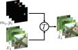
(a)

(b)

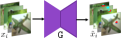
(c)

Figure 1: Illustrations of three approaches to model input-specific Trojan triggers $\psi_{i}=(m_{i},p_{i})$ w.r.t. $x_{i}$: as learnable parameters (a), via a trigger generator (b), and via a Trojan-image autoencoder (c).

Once trained, the Trojan-infected classifier $\mathtt{C}$ will be provided to victims (usually end-users) for deployment. When the victims test $\mathtt{C}$ with their own clean data, they do not see any abnormalities in performance because the Trojan remains dormant for the clean data. Thus, the victims naively believe that $\mathtt{C}$ is normal and use $\mathtt{C}$ as it is without any modification or additional safeguard.

3 Difficulty in Finding Input-Specific Triggers

In practice, we (as victims) usually have a small dataset $\mathcal{D}_{\text{val}}=\left\{(x_{i},y_{i})\right\}_{i=1}^{N_{\text{val}}}$ containing only clean samples for evaluating the performance of $\mathtt{C}$. We can leverage this set to find possible Trojan triggers associated with the target class $t$. For standard Trojan attacks [4, 11] that use only a global input-agnostic trigger $\psi=(m,p)$, $\psi$ can be restored by minimizing the following loss w.r.t. $m$ and $p$:

$$\mathcal{L}_{\text{gen}}(x,t)=-\log p_{\mathtt{C}}(t|\tilde{x})+\lambda_{0}\max(\|m\|-\delta,0),$$ (2)

where $(x,.)\sim\mathcal{D}_{\text{val}}$, $\tilde{x}$ is derived from $x$ via Eq. 1, $p_{\mathtt{C}}(t|\tilde{x})=\frac{\exp(\mathtt{C}_{t}(\tilde{x}))}{\sum_{k=1}^{K}\exp(\mathtt{C}_{k}(\tilde{x}))}$ is the probability of $\tilde{x}$ belonging to the target class $t$, $\|\cdot\|$ denotes a L1/L2 norm, $\delta\geq 0$ is an upper bound of the norm, and $\lambda_{0}\geq 0$ is a coefficient. The second term in Eq. 2 ensures that the trigger is small enough so that it could not be detected by human inspection. $\mathcal{L}_{\text{gen}}$ was used by Neural Cleanse (NC) [47] and its variants [3, 12, 13], and was shown to work well for standard attacks.

(a)

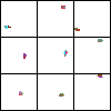
(b)

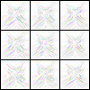
(c)

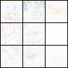
(d)

(e)

(f)

Figure 2: Trojan images (a) and the corresponding triggers (b) of an Input-Aware Attack. Triggers synthesized by Neural Cleanse (c) and by the three approaches in Fig. 1 (d, e, f). Trigger pixels are inverted for better visualization.

In this work, we however consider finding the triggers of Input-Aware Attack (InpAwAtk) [32]. This is a much harder problem because InpAwAtk uses different triggers $\psi_{i}=(m_{i},p_{i})$ for different input images $x_{i}$ instead of a global one. We examine 3 different ways to model $\psi_{i}$: (i) treating $m_{i},p_{i}$ as learnable parameters for each image $x_{i}\in\mathcal{D}_{\text{val}}$, (ii) via an input-conditional trigger generator $(m_{i},p_{i})=\mathtt{G}(x_{i})$, and (iii) generating a Trojan image $\tilde{x}_{i}$ w.r.t. $x_{i}$ via a Trojan-image generator $\tilde{x}_{i}=\mathtt{G}(x_{i})$ and treating $\tilde{x}_{i}-x_{i}$ as $\psi_{i}$. These are illustrated in Fig. 1. The first way does not generalize to other images not in $\mathcal{D}_{\text{val}}$ while the second and third do. We reuse the loss $\mathcal{L}_{\text{gen}}$ in Eq. 2 to learn $m_{i},p_{i}$ in the first way and $\mathtt{G}$ in the second way. The loss to train $\mathtt{G}$ in the third way is slightly adjusted from $\mathcal{L}_{\text{gen}}$ with $\|m\|$ replaced by $\|\tilde{x}-x\|$. As shown in Fig. 2, neither NC nor the above approaches can restore the original triggers of InpAwAtk, suggesting new methods are on demand.

4 Proposed Trojan Defenses

The great difficulty in finding correct input-specific triggers (Section 3) challenges a majority of existing Trojan defenses which assume a global input-agnostic trigger is applied to all input images [3, 8, 13, 22, 23, 35, 47]. Fortunately, although we may not be able to find correct triggers, in many cases, we can still design effective Trojan defenses by filtering out triggers embedded in the input without concerning about the number or the input dependence property of triggers. The fundamental idea is learning a filter network $\mathtt{F}$ that maps the original input image $x$ into a filtered image $x^{\circ}$, and using $x^{\circ}$ as input to the classifier $\mathtt{C}$ instead of $x$. In order for $\mathtt{F}$ to be considered as a good filter, $x^{\circ}$ should satisfy the following two conditions:

• Condition 1: If $x$ is clean, $x^{\circ}$ should look similar to $x$ and should have the same label as $x$’s. This ensures a high classification accuracy on clean images (dubbed “clean accuracy”).

• Condition 2: If $\tilde{x}$ contains triggers, $\tilde{x}^{\circ}$ should be close to $x$ and should have the same label as $x$’s where $x$ is the clean counterpart of $\tilde{x}$. This ensures a low attack success rate and a high clean-label recovery rate on Trojan images (dubbed “Trojan accuracy” and “recovery accuracy”, respectively).

In the next two subsections (4.1, 4.2), we propose two novel filtering defenses that leverage two different strategies to learn a good $\mathtt{F}$ which are lossy data compression and adversarial learning, respectively.

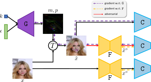
Figure 3: An illustration of Adversarial Input Filtering.

4.1 Variational Input Filtering

A natural choice for $\mathtt{F}$ is an autoencoder (AE) which should be complex enough so that $\mathtt{F}$ can reconstruct clean images well to achieve high clean accuracy. However, if $\mathtt{F}$ is too complex, it can capture every detail of a Trojan image including the embedded triggers, which also causes high Trojan accuracy. In general, an optimal $\mathtt{F}$ should achieve good balance between preserving class-related information and discarding noisy information of the input. To reduce the dependence of $\mathtt{F}$ on architecture, we propose to treat $\mathtt{F}$ as a variational autoencoder (VAE) [18] and train it with the “Variational Input Filtering” (VIF) loss given below:

$$\mathcal{L}_{\text{VIF}}(x,y)= -\log p_{\mathtt{C}}(y|x^{\circ})+\lambda_{1}\|x^{\circ}-x\|+\lambda_{2}D_{\text{KL}}(q_{\text{$\mathtt{F}$}}(z|x)\|p(z))$$ (3)

$$= \mathcal{L}_{\text{IF}}+\lambda_{2}D_{\text{KL}}(q_{\text{$\mathtt{F}$}}(z|x)\|p(z)),$$ (4)

where $(x,y)\sim\mathcal{D}_{\text{val}}$, $x^{\circ}=\mathrm{\mathtt{F}}(x)$ is the filtered version of $x$, $z$ is the latent variable, $q_{\mathtt{F}}(z|x)$ denotes the variational posterior distribution and is parameterized via the stochastic encoder of $\mathtt{F}$, $p(z)=\mathcal{N}(0,\mathrm{I})$ is the standard Gaussian distribution, $D_{\text{KL}}$ denotes the KL divergence, $\lambda_{1},\lambda_{2}\geq 0$ are coefficients. In Eq. 3, the first two terms force $\mathtt{F}$ to preserve class-related information of $x$ and to reduce the visual dissimilarity between $x^{\circ}$ and $x$ as per condition 1, 2. Meanwhile, the last term encourages $\mathtt{F}$ (or more precisely, $q_{\mathtt{F}}(z|x)$) to discard noisy information of $x$, which we refer to as “lossy data compression”. This can be explained via the following relationship [54]:

$$\mathbb{E}_{p(x)}\left[D_{\text{KL}}(q_{\mathtt{F}}(z|x)\|p(z))\right]=D_{\text{KL}}(q_{\mathtt{F}}(z)\|p(z))+I_{\text{$\mathtt{F}$}}(x,z),$$ (5)

where $q_{\mathtt{F}}(z)=\mathbb{E}_{p(x)}\left[q_{\mathtt{F}}(z|x)\right]$. Clearly, minimizing the LHS of Eq. 5 decreases the mutual information between $z$ and $x$. And because $z$ is used to compute $x^{\circ}$ (in decoding), this also reduces the information between $x^{\circ}$ and $x$.

In Eq. 3, the first two terms alone constitute the “Input Filtering” (IF) loss $\mathcal{L}_{\text{IF}}$. To the best of our knowledge, IF has not been proposed in other Trojan defense works. Input Processing (IP) [25] is the closest to IF but it is trained on unlabeled data using only the reconstruction loss (the second term in Eq. 3). In Appdx. 0.E.2, we show that IP performs worse than IF, which highlights the importance of the term $-\log p_{\mathtt{C}}(y|x^{\circ})$.

4.2 Adversarial Input Filtering

VIF, owing to its generality, do not make use of any Trojan-related knowledge in $\mathtt{C}$ to train $\mathtt{F}$. We argue that if $\mathtt{F}$ is exposed to such knowledge, $\mathtt{F}$ could be more selective in choosing which input information to discard, and hence, could perform better. This motivates us to use synthetic Trojan images as additional training data for $\mathtt{F}$ besides clean images from $\mathcal{D}_{\text{val}}$. We synthesize a Trojan image $\tilde{x}$ from a clean image $x$ as follows:

$$(m_{k},p_{k}) =\mathtt{G}(\epsilon,k),$$ (6)

$$\tilde{x} =T(x,(m_{k},p_{k})),$$ (7)

where $\epsilon\sim\mathcal{N}(0,\mathrm{I})$ is a standard Gaussian noise, $k$ is a class label sampled uniformly from $\mathcal{Y}$, $\mathtt{G}$ is a conditional generator, $T$ is the image blending function (Eq. 1). We choose the image blending function to craft Trojan images because it is the most general Trojan injection function (its output range spans the whole image space $\mathbb{I}^{c\times h\times w}$). To make sure that the synthetic Trojan images are useful for $\mathtt{F}$, we form an adversarial game between $\mathtt{G}$ and $\mathtt{F}$ in which $\mathtt{G}$ attempts to generate hard Trojan images that can fool $\mathtt{F}$ into producing the target class (sampled randomly from $\mathcal{Y}$) while $\mathtt{F}$ becomes more robust by correcting these images. We train $\mathtt{G}$ with the following loss:

$$\mathcal{L}_{\text{AIF-gen}}(x,k)=\mathcal{L}_{\text{gen}}(x,k)-\lambda_{3}\log p_{\mathtt{C}}(k|\tilde{x}^{\circ}),$$ (8)

where $\mathcal{L}_{\text{gen}}$ is similar to the one in Eq. 2 but with $m$ replaced by $m_{k}$ (Eq. 6), $\tilde{x}^{\circ}=\mathtt{F}(\tilde{x})$, $\lambda_{3}\geq 0$. The loss of $\mathtt{F}$ must conform to conditions 1, 2 and is:

$$\mathcal{L}_{\text{AIF}}(x,y)= \mathcal{L}_{\text{IF}}(x,y)-\lambda_{4}\log p_{\mathrm{\mathtt{C}}}(y|\tilde{x}^{\circ})+\lambda_{5}\|\tilde{x}^{\circ}-x\|$$ (9)

$$= \mathcal{L}_{\text{IF}}(x,y)+\mathcal{L}^{\prime}_{\text{IF}}(\tilde{x},y),$$ (10)

where AIF stands for “Adversarial Input Filtering”, $\mathcal{L}_{\text{IF}}$ was described in Eq. 4, $\tilde{x}$ is computed from $x$ via Eq. 7, $\lambda_{4},\lambda_{5}\geq 0$. Note that the last term in Eq. 10 is the reconstruction loss between $\tilde{x}^{\circ}$ and $x$ (not $\tilde{x}$). Thus, we denote the last two terms in Eq. 9 as $\mathcal{L}^{\prime}_{\text{IF}}$ instead of $\mathcal{L}_{\text{IF}}$. AIF is depicted in Fig. 3.

During experiment, we observed that sometimes training $\mathtt{G}$ and $\mathtt{F}$ with the above losses may not result in good performance. The reason is that when $\mathtt{F}$ becomes better, $\mathtt{G}$ tends to produce large-norm triggers to fool $\mathtt{F}$ despite the fact that a regularization was applied to the norms of these triggers. Large-norm triggers make learning $\mathtt{F}$ harder as $\tilde{x}$ is no longer close to $x$. To handle this problem, we explicitly normalize $m_{k}$ so that its norm is always bounded by $\delta$. We provide technical details and empirical study about this normalization in Appdx. 0.E.4.

4.3 Filtering then Contrasting

VIF and AIF always filter $x$ even when $x$ does not contain triggers, which often leads to the decrease in clean accuracy after filtering. To overcome this drawback, we introduce a new defense mechanism called “Filtering then Contrasting” (FtC) which works as follows: Instead of just computing the predicted label $\hat{y}^{\circ}$ of the filtered image $x^{\circ}=\mathtt{F}(x)$ and treat it as the final prediction, we also compute the predicted label $\hat{y}$ of $x$ without filtering and compare $\hat{y}$ with $\hat{y}^{\circ}$. If $\hat{y}$ is different from $\hat{y}^{\circ}$, $x$ will be marked as containing triggers and discarded. Otherwise, $x$ will be marked as clean and $\hat{y}$ will be used as the final prediction. FtC is especially useful for defending against attacks with large-norm triggers (Sect. 5.4.3) because it helps avoid the significant drop in clean accuracy caused by the large visual difference between $x^{\circ}$ and $x$. Under the FtC defense mechanism, we derive two new defenses VIFtC and AIFtC from VIF and AIF, respectively.

5 Experiments

5.1 Experimental Setup

Datasets

Following previous works [11, 32, 38], we evaluate our proposed defenses on four image datasets namely MNIST, CIFAR10 [19], GTSRB [42], and CelebA [26]. For CelebA, we follow Salem et al. [38] and select the top 3 most balanced binary attributes (out of 40) to form an 8-class classification problem. The chosen attributes are “Heavy Makeup”, “Mouth Slightly Open”, and “Smiling”. Like other works [8, 47], we assume that we have access to the test set of these datasets. We use 70% data of the test set for training our defense methods ($\mathcal{D}_{\text{val}}$ in Sections 3, 4) and 30% for testing (denoted as $\mathcal{D}_{\text{test}}$). For more details about the datasets, please refer to Appdx. 0.B.1. Sometimes, we do not test our methods on all images in $\mathcal{D}_{\text{test}}$ but on those not belonging to the target class. This set is denoted as $\mathcal{D}^{\prime}_{\text{test}}$. We also provide results with less training data in Appdx. 5.4.2.

Benchmark Attacks

We use 5 different benchmark Trojan attacks for our defenses, which are BadNet+, noise-BI+, image-BI+, InpAwAtk [32], and WaNet [33]. InpAwAtk and WaNet are recent SOTA attacks that were shown to break many strong defenses completely. BadNet+ and noise/image-BI+ are variants of BadNet [11] and Blended Injection (BI) [4] that use multiple triggers instead of one. They are described in detail in Appdx. 0.C.1. The training settings for the 5 attacks are given in Appdx. 0.B.2.

We also consider 2 attack modes namely single-target and all-target [32, 53]. In the first mode, only one class $t$ is chosen as target. Every Trojan image $\tilde{x}$ is classified as $t$ regardless of the ground-truth label of its clean counterpart $x$. Without loss of generality, $t$ is set to 0. In the second mode, $\tilde{x}$ is classified as $(k+1)\mod K$ if $x$ belongs to the class $k$. If not clearly stated, attacks are assumed to be single-target.

Dataset		Benign		BadNet+			noise-BI+			image-BI+			InpAwAtk				WaNet
		Clean		Clean	Trojan		Clean	Trojan		Clean	Trojan		Clean	Trojan	Cross		Clean	Trojan	Noise
MNIST		99.56		99.61	99.96		99.46	100.0		99.50	100.0		99.47	99.41	96.05		99.48	98.73	99.38
CIFAR10		94.82		94.88	100.0		94.69	100.0		95.15	99.96		94.58	99.43	88.68		94.32	99.59	92.58
GTSRB		99.72		99.34	100.0		99.30	100.0		99.18	100.0		98.90	99.54	95.19		99.12	99.54	99.03
CelebA		79.12		79.41	100.0		78.75	100.0		78.81	99.99		78.18	99.93	77.16		78.48	99.94	77.24

Table 1: Test clean and Trojan accuracies of various Trojan attacks.

We report the test clean and Trojan accuracies of the benchmark attacks (in single-target mode) in Table 5.1. It is clear that all attacks achieve very high Trojan accuracies with little or no decrease in clean accuracy compared to the benign model’s, hence, are qualified for our experimental purpose. For results of the attacks on $\mathcal{D}_{\text{test}}$, please refer to Appdx. 0.C.

Baseline Defenses

We consider 5 well-known baseline defenses namely Neural Cleanse (NC) [47], STRIP [8], Network Pruning (NP) [22], Neural Attention Distillation (NAD) [20], and Februus [5].

Neural Cleanse (NC) assumes that attacks (i) choose only one target class $t$ and (ii) use at least (not exactly) one input-agnostic trigger associated with $t$. We refer to (i) as the “single target class” assumption and (ii) as the “input-agnostic trigger” assumption. Based on these assumptions, NC finds a trigger $\psi_{k}=(m_{k},p_{k})$ for every class $k\in\mathcal{Y}$ via reverse-engineering (Eq. 2), and uses the L1 norms of the synthetic trigger masks $\{m_{1},...,m_{K}\}$ to detect the target class. The intuition is that if $t$ is the target class, ${\|m_{t}\|}_{1}$ will be much smaller than the rest. A $z$-value of each mask norm is calculated via Median Absolute Deviation and the $z$-value of the smallest mask norm (referred to as the anomaly index) is compared against a threshold $\zeta$ (2.0 by default). If the anomaly index is smaller than $\zeta$, $\mathtt{C}$ is marked as clean. Otherwise, $\mathtt{C}$ is marked Trojan-infected with the target class corresponding to the smallest mask norm. In this case, the Trojans in $\mathtt{C}$ can be mitigated via pruning or via checking the cleanliness of input images. Both mitigation methods make use of $\psi_{t}$ and are analyzed in Appdx. 0.D.

STRIP assumes triggers are input-agnostic and argues that if an input image $x$ contains triggers then these triggers still have effect if $x$ is superimposed (blended) with other images. Therefore, STRIP superimposes $x$ with $N_{\text{s}}$ random clean images from $\mathcal{D}_{\text{val}}$ and computes the average entropy $\mathcal{H}(x)$ of $N_{\text{s}}$ predicted class probabilities corresponding to $N_{\text{s}}$ superimposed versions of $x$. If $\mathcal{H}(x)$ is smaller than a predefined threshold, $x$ is considered as trigger-embedded, otherwise, clean. The threshold is set according to the false positive rate (FPR) over the average entropies of all images in $\mathcal{D}_{\text{val}}$, usually at FPR equal to 1/5/10%. We evaluate the performance of STRIP against an attack using $M_{\text{s}}$ random clean images from $\mathcal{D}_{\text{test}}$ and $M_{\text{s}}$ corresponding Trojan images generated by that attack. Following [8], we set $N_{\text{s}}=100$ and $M_{\text{s}}=2000$.

Network Pruning (NP) hypothesizes that idle neurons are more likely to store Trojan-related information. Thus, it ranks neurons in the second top layer of $\mathtt{C}$ according to their average activation over all data in $\mathcal{D}_{\text{val}}$ and gradually prunes them until a certain decrease in clean accuracy is reached, usually at 1/5/10% decrease in clean accuracy.

Neural Attention Distillation (NAD) [20] is a distillation-based Trojan defense. It first fine-tunes the pretrained classifier $\mathtt{C}$ on clean images in $\mathcal{D}_{\text{val}}$ to obtain a fine-tune classifier $\mathtt{T}$. Then, it treats $\mathtt{T}$ and $\mathtt{C}$ as the teacher and student respectively, and performs attention-based feature distillation [52] between $\mathtt{T}$ and $\mathtt{C}$ on $\mathcal{D}_{\text{val}}$ again. Since $\mathtt{T}$ is $\mathtt{C}$ fine-tuned on clean data, $\mathtt{T}$ is expected to have most of the Trojan in $\mathtt{C}$ removed. Via distillation, such Trojan-free knowledge is transferred from $\mathtt{T}$ to $\mathtt{C}$ while performance of $\mathtt{C}$ on clean data is still preserved.

Among the baselines, Februus is the most related to our filtering defenses since it mitigates Trojan attacks via input purification. It uses GradCAM [40] to detect regions in an input image $x$ that may contain triggers. Then, it removes all pixels in the suspected regions and generates new ones via inpainiting. The inpainted image is expected to contain no trigger and is fed to $\mathtt{C}$ instead of $x$.

Model Architectures and Training Settings

Please refer to Appdx. 0.B.3.

Metrics

We evaluate VIF/AIF using 3 metrics namely decrease in clean accuracy ($\downarrow$C), Trojan accuracy (T), and decrease in recovery accuracy ($\downarrow$R). The first is the difference between the classification accuracies of clean images before and after filtering. The second is the attack success rate of Trojan images after filtering. The last is the difference between the classification accuracy of clean images before filtering and that of the corresponding Trojan images after filtering. Smaller values of the metrics indicate better results. $\downarrow$C and $\downarrow$R are computed on $\mathcal{D}_{\text{test}}$. T is computed on $\mathcal{D}^{\prime}_{\text{test}}$ under single-target attacks and $\mathcal{D}_{\text{test}}$ under all-target attacks. This ensures that T can be $0$ in the best case. Otherwise, T will be around $1/K$ where $K$ is the total number of classes. $\downarrow$C and $\downarrow$R are upper-bounded by 1 and can be negative.

We evaluate VIFtC/AIFtC using FPR and FNR. FPR/FNR is defined as the proportion of clean/Trojan images having different/similar class predictions when the filter $\mathtt{F}$ is applied and not applied. FPR is computed on $\mathcal{D}_{\text{test}}$. FNR is computed on $\mathcal{D}^{\prime}_{\text{test}}$ under single-target attacks and $\mathcal{D}_{\text{test}}$ under all-target attacks. Both metrics are in [0, 1] and smaller values of them are better. Interestingly, FPR and FNR are strongly correlated to $\downarrow$C and T, respectively. FPR/FNR is exactly equal to $\downarrow$C/T if $\mathtt{C}$ achieves perfect clean/Trojan accuracy.

5.2 Results of Baseline Defenses

(a) Neural Cleanse

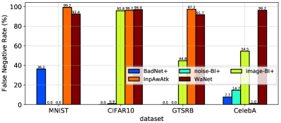
(b) STRIP

Figure 4: (a) Anomaly indices of Neural Cleanse. The red dashed line indicates the threshold. (b) FNRs of STRIP at 10% FPR.

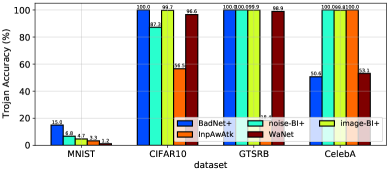
(a) Network Pruning

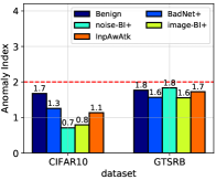
(b) Neural Cleanse

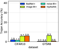
(c) VIF

Figure 5: (a) Trojan accuracies at 10% decrease in clean accuracy of different Trojan classifiers pruned by Network Pruning. (b) Anomaly indices of NC and (c) Trojan accuracies of VIF against all-target attacks on CIFAR10 and GTSRB.

In Fig. 4, we show the detection results of Neural Cleanse (NC) and STRIP w.r.t. the aforementioned attacks. The two defenses are effective against BadNet+ and image/noise-BI+. This is because STRIP and NC generally do not make any assumption about the number of triggers. However, STRIP performs poorly against InpAwAtk and WaNet (FNRs > 90%) since these advanced attacks break its “input-agnostic trigger” assumption. NC also fails to detect the Trojan classifiers trained by WaNet on most datasets for the same reason. What surprises us is that in our experiment NC correctly detect the Trojan classifiers trained by InpAwAtk on 3/4 datasets while in the original paper [32], it was shown to fail completely. We are confident that this inconsistency does not come from our implementation of InpAwAtk since we used the same hyperparameters and achieved the same classification results as those in the original paper (Table 5.1 versus Fig. 3b in [32]). However, NC is still unable to mitigate all Trojans in these correctly-detected Trojan classifiers (Appdx. 0.D.3). In addition, as shown in Fig. 5b, NC is totally vulnerable to all-target attacks since its “single target class” assumption is no longer valid under these attacks. Network Pruning (NP), despite being assumption-free, cannot mitigate Trojans from most attacks (high Trojan accuracies in Fig. 5a) as it fails to prune the correct neurons containing Trojans. Februus has certain effects on mitigating Trojans from BadNet+ while being useless against the remaining attacks (high Ts in Table 5.3). This is because GradCAM, the method used by Februus, is only suitable for detecting patch-like triggers of BadNet+, not full-size noise-like triggers of image/noise-BI+ or polymorphic triggers of InpAwAtk/WaNet. We also observe that Februus significantly reduces the clean accuracy (high $\downarrow$Cs in Table 5.3) as it removes input regions that contain no Trojan trigger yet are highly associated with the output class. This problem, however, was not discussed in the Februus paper. NAD, thanks to its distillation-based nature, usually achieves better clean accuracies than our filtering defenses (Table 5.3). This defense is also effective against InpAwAtk and WaNet. However, NAD performs poorly in recovering Trojan samples from BadNet+ and noise/image-BI+ (high $\downarrow$Rs), especially on MNIST. Besides, NAD is much less robust to large-norm triggers than our filtering defenses (Sect. 5.4.3). For more analyses of the baseline defenses, please refer to Appdx. 0.D.

5.3 Results of Proposed Defenses

Dataset	Defense	Benign	BadNet+			noise-BI+			image-BI+			InpAwAtk			WaNet
		$\downarrow$C	$\downarrow$C	T	$\downarrow$R	$\downarrow$C	T	$\downarrow$R	$\downarrow$C	T	$\downarrow$R	$\downarrow$C	T	$\downarrow$R	$\downarrow$C	T	$\downarrow$R
MNIST	Feb.	5.96	39.08	96.24	86.32	2.30	100.0	89.58	8.19	100.0	89.58	9.90	92.40	83.32	25.43	80.46	88.75
	NAD	0.45	0.82	35.72	36.41	0.75	84.83	76.22	0.78	88.34	79.18	0.80	4.46	5.29	0.42	0.44	0.98
	IF	0.10	0.27	2.47	4.99	0.10	0.16	13.52	0.13	1.29	12.02	0.21	0.96	2.08	0.23	0.34	0.61
	VIF	0.13	0.17	2.36	3.63	0.12	0.04	0.63	0.03	0.11	0.40	0.20	1.25	1.83	0.10	0.48	0.53
	AIF	0.10	0.17	3.80	4.86	0.13	0.15	0.11	0.10	0.11	0.10	0.03	1.14	1.66	0.13	0.15	0.20
CIFAR10	Feb.	32.67	49.17	12.63	19.57	26.73	43.59	78.90	39.70	92.67	81.00	53.43	49.52	66.50	55.80	98.70	83.30
	NAD	3.16	3.81	35.71	41.68	2.52	1.81	28.89	3.87	1.63	18.92	2.98	1.81	4.75	2.95	0.93	5.42
	IF	3.34	4.15	2.30	7.79	3.32	1.01	4.43	4.76	37.48	34.30	4.47	16.35	18.96	3.21	4.82	6.80
	VIF	7.81	7.70	2.52	11.27	6.43	1.22	7.10	7.53	10.52	16.50	7.67	3.07	12.38	7.97	3.96	10.67
	AIF	4.67	5.60	2.37	9.03	4.87	1.14	6.02	5.23	1.96	7.10	5.28	5.30	11.87	4.30	1.22	5.67
GTSRB	Feb.	42.01	35.30	21.02	44.11	43.40	75.75	95.90	32.18	97.83	97.37	21.27	70.02	72.71	33.18	70.10	71.69
	NAD	-0.13	-0.35	0.00	8.20	-0.32	0.00	4.06	-0.42	0.05	8.33	-0.28	0.05	0.56	-0.40	0.00	0.11
	IF	0.12	0.13	0.00	2.55	0.13	0.03	1.52	0.37	52.27	51.95	0.03	0.66	3.60	0.08	9.83	9.62
	VIF	0.18	0.45	0.00	3.55	0.18	0.00	1.12	0.37	12.12	16.56	0.11	0.03	1.87	0.55	3.67	3.89
	AIF	0.05	-0.16	0.00	1.87	0.05	0.00	0.81	0.13	7.47	9.54	-0.03	0.05	1.37	-0.05	0.50	0.42
CelebA	Feb.	12.71	18.80	42.96	21.33	11.76	93.27	49.05	13.30	98.59	49.84	5.60	99.98	49.71	9.16	97.30	48.53
	NAD	3.06	3.19	12.14	9.98	3.56	25.31	23.07	3.51	16.97	9.46	3.14	13.85	11.24	2.51	11.48	3.21
	IF	2.23	4.21	8.62	4.75	2.57	13.83	6.00	2.25	59.39	27.94	2.86	11.95	6.07	2.43	15.21	4.75
	VIF	3.74	4.63	9.28	4.90	3.20	11.51	4.08	3.54	14.32	5.62	3.89	11.55	6.27	3.96	8.30	4.19
	AIF	4.95	6.46	7.85	6.49	4.18	12.56	6.52	4.37	18.40	9.23	3.71	10.43	7.65	4.02	12.82	5.74

Table 2: Trojan filtering results (in %) of Februus, NAD, and our filtering defenses against different attacks. Smaller values are better. For a particular dataset, attack, and metric, the best defense is highlighted in bold.

From Table 5.3, it is clear that VIF and AIF achieve superior performances in mitigating Trojans of all the single-target attacks compared to most of the baseline defenses. For example, on MNIST and GTSRB, our filtering defenses impressively reduce T from about 100% (Table 5.1) to less than 2% for most attacks yet only cause less than 1% drop of clean accuracy ($\downarrow$C < 1%). On more diverse datasets such as CIFAR10 and CelebA, VIF and AIF still achieve T less than 6% and 12% for most attacks while maintaining $\downarrow$C below 8% and 5%, respectively. We note that on CelebA, the nonoptimal performance of $\mathtt{C}$ (accuracy $\approx$ 79%) makes T higher than normal because T may contains the error of samples from non-target classes misclassified as the target class. However, it is not trivial to disentangle the two quantities so we leave this problem for future work. As there is no free lunch, our filtering defenses may be not as good as some baselines in some specific cases. For example, on CIFAR10, STRIP achieves FNRs $\approx$ 0% against BadNet+/noise-BI+ (Fig. 4b) while VIF/AIF achieves Ts $\approx$ 1-3%. However, the gaps are very small and in general, our filtering defenses are still much more effective than the baseline defenses against all the single-target attacks. Our filtering defenses also perform well against all-target attacks (Fig. 5c and Appdx. 0.E.1) as ours are not sensitive to the number of target classes. To gain a better insight into the performance of VIF/AIF, we visualize the filtered images produced by VIF/AIF and their corresponding “counter-triggers” in Appdx. 0.F.1.

Dataset	Defense	Benign	BadNet+		noise-BI+		image-BI+		InpAwAtk		WaNet
		FPR	FPR	FNR	FPR	FNR	FPR	FNR	FPR	FNR	FPR	FNR
MNIST	IFtC	0.40	0.50	2.21	0.37	0.22	0.37	1.51	0.53	1.71	0.60	1.33
	VIFtC	0.27	0.30	2.84	0.23	0.07	0.40	0.15	0.47	1.99	0.30	1.51
	AIFtC	0.23	0.32	4.17	0.17	0.15	0.17	0.11	0.33	1.87	0.13	1.18
CIFAR10	IFtC	6.83	7.47	1.70	6.57	0.93	7.83	36.56	7.25	16.89	7.17	5.15
	VIFtC	12.30	11.00	2.63	10.67	1.26	11.03	10.89	10.63	3.67	11.40	4.26
	AIFtC	8.63	8.87	1.96	8.73	0.89	8.77	2.15	8.27	5.93	7.93	1.56
GTSRB	IFtC	0.38	0.45	0.00	0.24	0.03	0.66	52.91	0.29	1.00	0.66	10.41
	VIFtC	0.45	0.74	0.03	0.47	0.00	0.87	12.63	0.53	0.37	1.31	4.25
	AIFtC	0.50	0.37	0.03	0.39	0.00	0.63	7.87	0.47	0.40	0.60	1.08
CelebA	IFtC	14.24	15.78	8.36	14.94	14.25	13.99	59.43	12.84	11.95	13.08	15.27
	VIFtC	17.74	18.90	9.09	18.50	11.67	18.09	14.30	16.37	11.54	17.22	8.34
	AIFtC	20.24	20.95	7.71	19.08	12.82	19.29	18.65	16.54	10.43	16.55	12.87

Table 3: Trojan mitigation results (in %) of our FtC defenses against different attacks. Smaller values are better. For a particular attack, dataset, and metric, the best defense is highlighted in bold.

Among the filtering defenses, IF usually achieves the smallest $\downarrow$Cs because its loss does not have any term that encourages information removal like VIF’s and AIF’s. The gaps in $\downarrow$C between IF and AIF/VIF are the largest on CIFAR10 but do not exceed 5%. However, IF usually performs much worse than VIF/AIF in mitigating Trojans, especially those from image-BI+, InpAwAtk, and WaNet. For example, on CIFAR10, GTSRB, and CelebA, IF reduces the attack success rate (T) of image-BI+ to 37.48%, 52.27%, and 59.39% respectively. These numbers are only 1.96%, 7.47%, and 18.40% for AIF and 10.52%, 12.12%, and 14.32% for VIF. Therefore, when considering the trade-off between $\downarrow$C and T, VIF and AIF are clearly better than IF. We also observe that AIF usually achieves lower $\downarrow$Cs and $\downarrow$Rs than VIF. It is because AIF discards only potential malicious information instead of all noisy information like VIF. However, VIF is simpler and easier to train than AIF.

From Table 5.3, we see that the FPRs and FNRs of VIFtC/AIFtC are close to the $\downarrow$Cs and Ts of VIF/AIF respectively on MNIST, GTSRB, and CIFAR10. This is because $\mathtt{C}$ achieves nearly 100% clean and Trojan accuracies on these datasets. Thus, we can interpret the results of VIFtC/AIFtC in the same way as what we have done for VIF/AIF. Since FPR only affects the classification throughput not (clean) accuracy, VIFtC/AIFtC are preferred to VIF/AIF in applications that favor (clean) accuracy (e.g., defending against attacks with large-norm triggers in Sect. 5.4.3).

5.4 Ablation Studies

It is undoubted that our defenses require some settings to work well. However, these settings cannot be managed by attackers unlike the assumptions of most existing defenses [8, 47]. Below, we examine the contribution of lossy data compression to the performance of VIF, and the robustness of our proposed defenses to small amounts of training data and to large-norm triggers. For other ablation studies, please refer to Appdx. 0.E.

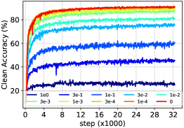
(a) Clean Accuracy

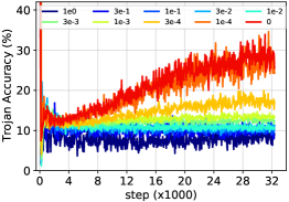
(b) Trojan Accuracy

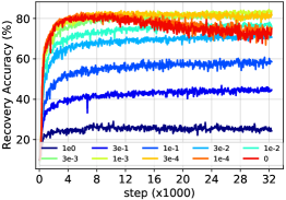
(c) Recovery Accuracy

Figure 6: Clean, Trojan, and recovery accuracy curves of VIF against InpAwAtk on CIFAR10 w.r.t. different values of $\lambda_{2}$ in Eq. 3. The Trojan accuracy curves in (b) fluctuate around 10% since they are computed on $\mathcal{D}_{\text{test}}$ instead of $\mathcal{D}^{\prime}_{\text{test}}$.

5.4.1 Different data compression rates in VIF

The lossy data compression in VIF can be managed via changing the coefficients of $D_{\text{KL}}$ in $\mathcal{L}_{\text{VIF}}$ ($\lambda_{2}$ in Eq. 3). A smaller values of $\lambda_{2}$ means a lower data compression rate and vice versa. From Fig. 6, it is clear that when $\lambda_{2}$ is small, most information in the input including both semantic information and embedded triggers is retained, thus, the clean accuracy (C) and the Trojan accuracy (T) are both high. To decide the optimal value of $\lambda_{2}$, we base on recovery accuracy (R) since R can be seen as a combination of C and T to some extent. From the results on CIFAR10 (Fig. 6) and on other datasets, we found $\lambda_{2}=0.003$ to be the best.

Def.	Metric	InpAwAtk
		Default	Fixed #epochs						Fixed total #iterations
		1.0	0.8	0.6	0.4	0.2	0.1	0.05	0.8	0.6	0.4	0.2	0.1	0.05
	$\downarrow$C	4.47	4.73	4.43	5.37	7.90	11.60	25.93	3.53	3.87	3.83	4.20	4.23	4.87
IF	T	16.35	15.11	11.56	9.48	6.70	4.07	6.70	16.11	15.41	20.22	18.37	26.33	21.00
	$\downarrow$R	18.96	19.00	15.10	15.47	15.07	17.47	32.23	18.47	18.03	21.87	20.57	26.63	23.17
	$\downarrow$C	7.67	9.17	8.57	9.83	12.13	17.10	27.80	8.53	7.93	7.87	8.97	9.37	11.27
VIF	T	3.07	3.81	2.81	4.30	3.30	2.70	5.67	3.26	4.19	4.26	3.70	3.44	4.67
	$\downarrow$R	12.38	14.90	13.17	16.30	17.37	22.10	32.30	13.73	13.87	13.67	14.73	15.03	17.87
	$\downarrow$C	5.28	5.47	6.53	7.90	11.70	16.67	26.13	5.07	5.23	5.17	6.17	5.77	7.83
AIF	T	5.30	4.96	3.59	4.89	3.15	2.89	4.00	6.63	9.04	5.70	4.56	8.48	12.96
	$\downarrow$R	11.87	11.60	11.90	13.87	17.03	21.80	30.40	11.73	13.83	11.77	12.57	14.50	19.93

Table 4: Trojan filtering results (in %) of IF, VIF, and AIF against InpAwAtk on CIFAR10 w.r.t. different proportions of training data (the third row) and two broader training settings (the second row): i) fixed number of epochs, and ii) fixed total number of iterations. Results taken from Table 5.3 are shown in italic.

	Fixed #epochs		Fixed total #iterations
		width 2pt
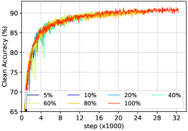
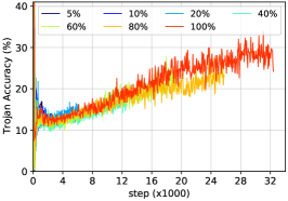
IF		width 2pt
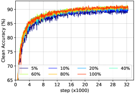
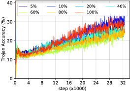
		width 2pt
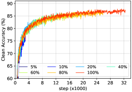
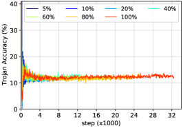
VIF		width 2pt
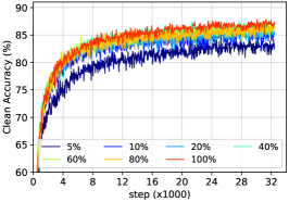
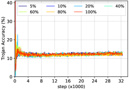
		width 2pt
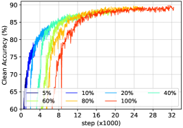
AIF		width 2pt

Figure 7: Test clean accuracy and Trojan accuracy curves of our filtering defenses (IF, VIF, AIF) against InpAwAtk on CIFAR10 w.r.t. different proportions of training data and 2 broader training settings: i) fixed number of epochs and ii) fixed total number of iterations.

5.4.2 Robustness to small amounts of training data

We are curious to know how well our proposed defenses will perform if we reduce the amount of training data. We select the proportion of training data from {0.8, 0.6, 0.4, 0.2, 0.1, 0.05}. In addition, we consider two broader training settings. In the first setting, the number of training epochs is fixed at 600 (Section 0.B.3) regardless of the amount of training data. Because less training data results in fewer iterations per epoch, fixing the number of training epochs means smaller total number of training iterations for less training data. In the second setting, we adjust the number of training epochs based on the proportion of training data so that the total number of training iterations is fixed and similar to that when full data is used. Table 5.4.1 shows the results of our filtering defenses w.r.t. the above settings. When the number of epochs is fixed, we see that our defenses often achieve lower Ts yet larger $\downarrow$Cs (and $\downarrow$Rs) for less training data. This is because the filter $\mathtt{F}$ has not been fully trained to reconstruct the input image well enough (the first column in Fig. 5.4.1). On the other hand, when the total number of iterations is fixed, $\mathtt{F}$ has been fully trained and we do not see much difference in Trojan accuracy of VIF for different amounts of training data. The Trojan accuracy of AIF slightly increase for less training data but is still acceptable (the last column in Fig. 5.4.1). Changes in clean accuracy of our filtering defenses are small (the third column in Fig. 5.4.1). In summary, these results suggest that our filtering defenses are quite robust to the limited amount of training data.

5.4.3 Robustness to large-norm triggers

In this section, we examine the performances of our defenses against attacks that use large-norm triggers. We consider BadNet+ and noise-BI+ for this study. For BadNet+, we increase the trigger norm by increasing the trigger size $s$. The results for BadNet+ are shown in Table 5.4.3. For noise-BI+, we increase the trigger norm by increasing the blending ratio $\alpha$. The results for noise-BI+ are shown in Table 5.4.3. It is clear that even when triggers have large norms, our filtering defenses, especially VIF, still effectively erase most of the trigger pixels that could activate the Trojans in $\mathtt{C}$ (Fig. 25) and achieve low Trojan accuracies (Tables. 5.4.3, 5.4.3). However, large-norm triggers cause a lot of difficulty in reconstructing the original clean images from Trojan images (Fig. 25), which leads to large decreases in recovery accuracy of our methods. Note that such poor performance is inevitable for filtering defenses like VIF and AIF. A solution to this problem is using other types of defenses. STRIP [8], Neural Cleanse [47], and NAD [20] are possible yet not good options. As shown in Fig. 5.4.3, STRIP works well against BadNet+ with large trigger sizes but poorly against noise-BI+ with large blending ratios. We guess the reason is that with large blending ratios, Trojan images of noise-BI+ will look like noises, and superimposing a noise-like Trojan image with a clean image is like adding noise to the clean image, hence, won’t affect of the class prediction of the clean image. Neural Cleanse tends to wrongly identify Trojan models as benign if the behind attacks use triggers with large enough norms. This is because the reverse-engineered trigger w.r.t. the true target class also has large norm which is not very different from the norms of the reverse-engineered triggers w.r.t. other classes. NAD achieves impracticably high Trojan accuracies when trigger norms are large for both BadNet+ and noise-BI+. By contrast, our FtC defenses, especially VIFtC, are good alternatives. VIFtC achieves very low FNRs (<7% in case of BadNet+ and <2% in case of noise-BI+) while still keeping FPRs in an acceptable range between 10% and 15% (Tables. 5.4.3, 5.4.3).

Defense	BadNet+
	$s=5$					$s=11$					$s=17$					$s=23$
	$\downarrow$C	T	$\downarrow$R	FPR	FNR	$\downarrow$C	T	$\downarrow$R	FPR	FNR	$\downarrow$C	T	$\downarrow$R	FPR	FNR	$\downarrow$C	T	$\downarrow$R	FPR	FNR
IF | IFtC	4.15	2.30	7.79	7.47	1.70	5.83	6.33	29.27	8.83	6.81	4.17	22.52	52.50	6.83	22.37	4.30	64.41	78.77	7.47	63.74
VIF | VIFtC	7.70	2.52	11.27	11.00	2.63	11.07	3.89	31.07	14.43	3.85	9.13	5.41	55.60	12.80	4.89	9.77	7.22	77.73	14.07	6.81
AIF | AIFtC	5.60	2.37	9.03	8.87	1.96	5.53	3.33	23.97	9.03	3.15	4.67	7.56	48.40	8.30	8.04	5.10	28.07	77.70	8.30	28.0
AIF∗ | AIFtC∗	5.90	2.15	10.00	9.30	2.15	6.50	5.00	34.33	9.97	5.30	5.77	14.63	52.67	9.33	13.70	6.97	29.96	77.93	10.60	30.19

Table 5: Trojan filtering results (in %) of IF, VIF, AIF, and AIF without explicit trigger normalization (AIF^∗) against BadNet+ with different trigger sizes ($s$) on CIFAR10. For a particular trigger size and metric, the best result is highlighted in bold. Results taken from Tables 5.3, 5.3 are shown in italic.

Defense	noise-BI+
	$\alpha=0.1$					$\alpha=0.3$					$\alpha=0.5$					$\alpha=0.7$
	$\downarrow$C	T	$\downarrow$R	FNR	FPR	$\downarrow$C	T	$\downarrow$R	FNR	FPR	$\downarrow$C	T	$\downarrow$R	FNR	FPR	$\downarrow$C	T	$\downarrow$R	FNR	FPR
IF/IFtC	3.32	1.01	4.43	6.57	0.93	4.30	1.26	36.73	7.80	1.19	3.53	27.59	73.03	7.10	26.74	3.87	49.37	83.10	7.13	49.00
VIF/VIFtC	6.43	1.22	7.10	10.67	1.26	7.53	1.44	27.57	11.80	1.56	7.67	0.74	67.33	11.63	0.74	7.93	0.22	80.80	11.57	0.26
AIF/AIFtC	4.87	1.14	6.02	8.73	0.89	4.90	1.33	39.50	8.60	1.37	5.30	7.00	72.30	9.10	7.11	6.07	31.41	80.70	8.87	31.67
AIF∗/AIFtC∗	5.60	0.78	7.50	9.53	0.74	6.07	0.48	45.13	10.10	0.74	6.27	1.48	74.83	10.67	1.78	6.47	38.74	80.97	10.00	39.56

Table 6: Trojan filtering results (in %) of IF, VIF, AIF, and AIF without explicit trigger normalization (AIF^∗) against noise-BI+ with different blending ratios ($\alpha$) on CIFAR10. For a particular blending ratio and metric, the best result is highlighted in bold. Results taken from Tables 5.3, 5.3 are shown in italic.

	STRIP	Neural Cleanse	NAD	AIF	VIF
BadNet+
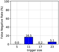
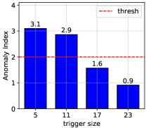
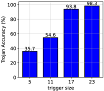
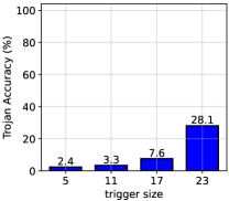
noise-BI+

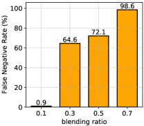
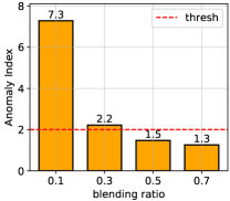
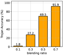
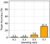
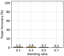
Figure 8: FNRs at 10% FPR of STRIP, anomaly indices of Neural Cleanse, Trojan accuracies of NAD, and Trojan accuracies of our filtering defenses VIF, AIF against BadNet+ with different trigger sizes (top) and noise-BI+ with different blending ratios (bottom).

6 Related Work

Due to space limit, in this section we only discuss related work about Trojan defenses. Related work about Trojan attacks are provided in Appdx. 0.A. A large number of Trojan defenses have been proposed so far, among which Neural Cleanse (NC) [47], Network Pruning (NP) [22], STRIP [8], Neural Attention Distillation (NAD) [20], and Februus [5] are representative for five different types of defenses and are carefully analyzed in Section 5.1. DeepInspect [3], MESA [35] improve upon NC by synthesizing a distribution of triggers for each class instead of just a single one. TABOR [12] adds more regularization losses to NC to better handle large and scattered triggers. STS [13] restores triggers by minimizing a novel loss function which is the pairwise difference between the class probabilities of two random synthetic Trojan images. This makes STS independent of the number of classes and more efficient than NC on datasets with many classes. ABS [23] is a quite complicated defense inspired by brain stimulation. It analyzes all neurons in the classifier $\mathtt{C}$ to find “compromised” ones and use these neurons to validate whether $\mathtt{C}$ is attacked or not. DL-TND [48], B3D [6] focus on detecting Trojan-infected models in case validation data are limited. However, all the aforementioned defenses derived from NC still make the same “input-agnostic trigger” and “single target class” assumptions as NC, and hence, are supposed to be ineffective against attacks that break these assumptions such as input-specific [32, 33] and all-target attacks. Activation Clustering [2] and Spectral Signatures [45] regard hidden activations as a clue to detect Trojan samples from BadNet [11]. They base on an empirical observation that the hidden activations of Trojan samples and clean samples of the target class usually form distinct clusters in the hidden activation space. These defenses are of the same kind as STRIP and are not applicable to all-target attacks. Mode Connectivity Repair (MCR) [53] mitigates Trojans by choosing an interpolated model near the two end points of a parametric path connecting a Trojan model and its fine-tuned version. MCR was shown to be defeated by InpAwAtk in [32]. Adversarial Neuron Pruning (ANP) [50] leverages adversarial learning to find compromised neurons for pruning. Our AIF is different from ANP in the sense that we use adversarial learning to train an entire generator $\mathtt{G}$ for filtering input instead of pruning neurons.

7 Conclusion

We have proposed two novel “filtering” Trojan defenses dubbed VIF and AIF that leverage lossy data compression and adversarial learning respectively to effectively remove all potential Trojan triggers embedded in the input. We have also introduced a new defense mechanism called “Filtering-then-Contrasting” (FtC) that circumvents the loss in clean accuracy caused by “filtering”. Unlike most existing defenses, our proposed filtering and FtC defenses make no assumption about the number of triggers/target classes or the input dependency property of triggers. Through extensive experiments, we have demonstrated that our proposed defenses significantly outperform many well-known defenses in mitigating various strong attacks. In the future, we would like to extend our proposed defenses to other domains (e.g., texts, graphs) and other tasks (e.g., object detection, visual reasoning) which we believe are more challenging than those considered in this work.

Acknowledgement

This research was partially supported by the Australian Government through the Australian Research Council’s Discovery Projects funding scheme (project DP210102798). The views expressed herein are those of the authors and are not necessarily those of the Australian Government or Australian Research Council.

Table of Content for Appendix

1. 1 Introduction
2. 2 Standard Trojan Attack
3. 3 Difficulty in Finding Input-Specific Triggers
4. 4 Proposed Trojan Defenses
   1. 4.1 Variational Input Filtering
   2. 4.2 Adversarial Input Filtering
   3. 4.3 Filtering then Contrasting
5. 5 Experiments
   1. 5.1 Experimental Setup
      1. 5.2 Results of Baseline Defenses
         1. 5.3 Results of Proposed Defenses
            1. 5.4 Ablation Studies
               1. 5.4.1 Different data compression rates in VIF
                  1. 5.4.2 Robustness to small amounts of training data
                     1. 5.4.3 Robustness to large-norm triggers
                        1. 6 Related Work
                           1. 7 Conclusion
                              1. 0.A Related Work about Trojan Attacks
                              2. 0.B Experimental Setup
                                 1. 0.B.1 Datasets
                                 2. 0.B.2 Model Architectures and Training Settings for Benchmark Attacks
                                    1. 0.B.3 Model Architectures and Training Settings for Our Defenses
                                       1. 0.C Additional Results of Benchmark Attacks
                                          1. 0.C.1 BadNet+ and Noise/Image-BI+
                                             1. 0.C.2 Results of Benchmark Attacks on $\mathcal{D}_{\text{test}}$
                                                1. 0.D Additional Results of Baseline Defenses
                                                   1. 0.D.1 Network Pruning
                                                      1. 0.D.2 STRIP
                                                         1. 0.D.3 Neural Cleanse
                                                            1. 0.D.4 Februus
                                                               1. 0.D.5 Neural Attention Distillation
                                                                  1. 0.E Additional Results and Ablation Studies of Our Defenses
                                                                     1. 0.E.1 Results of Our Defenses against All-target Attacks
                                                                        1. 0.E.2 Comparison between Input Filtering and Input Processing [25]
                                                                           1. 0.E.3 Different architectures of the filter $\mathtt{F}$
                                                                              1. 0.E.4 Explicit Normalization of Triggers in AIF
                                                                                 1. 0.E.4.1 Theoretical Derivation
                                                                                    1. 0.E.4.2 Empirical Results
                                                                                       1. 0.F Qualitative Results of Our Defenses
                                                                                          1. 0.F.1 Against Benchmark Attacks
                                                                                          2. 0.F.2 Against Attacks with Large-Norm Triggers

Appendix 0.A Related Work about Trojan Attacks

In this paper, we mainly consider a class of Trojan attacks in which attackers fully control the training processes of a classifier. We refer to these attacks as “full-control” attacks. There is another less common type of Trojan attacks called “clean-label” attacks [37, 41, 55]. These attacks assume a scenario in which people want to adapt a popular pretrained classifier $\mathtt{C}$ (e.g., ResNet [14]) for their tasks by retraining the top layers of $\mathtt{C}$ with additional data collected from the web. The goal of an attacker is to craft a poisoning image $\tilde{x}$ that looks visually indistinguishable from an image $x_{t}$ of the target class $t$ while being close to some source image $x_{s}$ in the feature space by optimizing the following objective:

$$\tilde{x}=\underset{x}{\text{argmin }}{\|\mathtt{C}_{\text{f}}(x)-\mathtt{C}_{\text{f}}(x_{s})\|}_{2}^{2}+\lambda{\|x-x_{t}\|}_{2}^{2}$$

where $\mathtt{C}_{\text{f}}(\cdot)$ denotes the output of the penultimate layer of $\mathtt{C}$. The attacker then puts $\tilde{x}$ on the web so that it can be collected and labeled by victims. Since $\tilde{x}$ looks like an image of the target class $t$, $\tilde{x}$ will be labeled as $t$. When the victims retrain $\mathtt{C}$ using a dataset containing $\tilde{x}$, $\tilde{x}$ will create a “backdoor” in $\mathtt{C}$. The attacker can use $x_{s}$ to access this “backdoor” and forces $\mathtt{C}$ to output $t$. Apart from the advantage that the attacker does not need to control the labeling process (while in fact, he can’t), the clean-label attack has several drawbacks due to its impractical assumptions. For example, the victims may retrain the whole $\mathtt{C}$ instead of just the last softmax layer of $\mathtt{C}$; the victims may use their own training data to which the attacker can’t access; the victims may use $\mathtt{C}$ for a completely new task that the attacker does not know; the attacker doesn’t even know who are the victims. Moreover, since $x_{s}$ often looks very different from images of the target class $t$, $x_{s}$ can be easily detected by human inspection at test time.

Compared to clean-label attacks, full-control attacks are much harder to defend against because attackers have all freedom to do whatever they want with $\mathtt{C}$ before sending it to the victims. BadNet [11], Blended Injection [4] are among the earliest attacks [16, 25] of this type that use only one global trigger and use image blending as an injection function. These attacks can be mitigated by well-known defenses like Neural Cleanse [47] or STRIP. Besides, their triggers also look unnatural. Therefore, subsequent attacks focus mainly on improving the robustness and stealthiness of triggers at test time. Some attacks use dynamic and/or input-specific triggers [21, 32, 33, 38]. Others use more advanced injection functions [24, 33] or GANs [31] to create hidden triggers or use physical objects as triggers [4, 49].

Appendix 0.B Experimental Setup

Dataset	#Classes	Image size	Attack		Defense
			#Train	#Test	#Train	#Test
MNIST	10	28$\times$28$\times$1	60000	10000	7000	3000
CIFAR10	10	32$\times$32$\times$3	50000	10000	7000	3000
GTSRB	43	32$\times$32$\times$3	39209	12630	8826	3804
CelebA	8	64$\times$64$\times$3	162770	19867	13904	5963

Table 7: Datasets used in our experiments.

0.B.1 Datasets

We provide details of the datasets used in our experiments in Table 7. The training and test sets for defense ($\mathcal{D}_{\text{val}}$ and $\mathcal{D}_{\text{test}}$) are taken from the test set for attack with the #training/#test ratio of 0.7/0.3.

Encoder	Encoder
ConvBlockX(1, 16)	ConvBlockY(3, 64)
ConvBlockX(16, 32)	ConvBlockY(64, 128)
ConvBlockX(32, 64)	ConvBlockY(128, 256)
Reshape [64, 3, 3] to [576]	ConvBlockY(256, 512)
LinearBlockX(576, 256)
Decoder	Decoder
LinearBlockX(256, 576)	DeconvBlockY(512, 512)
Reshape [576] to [64, 3, 3]	DeconvBlockY(512, 256)
DeconvBlockX(64, 32)	DeconvBlockY(256, 128)
DeconvBlockX(32, 16)	DeconvBlockY(128, 3)
DeconvBlockX(16, 1)
MNIST	CelebA

Table 8: Architectures of $\mathtt{F}$ (in AIF) for MNIST and CelebA.

LinearBlockX($d_{i}$ ,$d_{o}$)
Linear($d_{i}$, $d_{o}$, $b$=False)
BatchNorm2d($d_{o}$, $m$=0.01)
ReLU()
ConvBlockX($c_{i}$, $c_{o}$)	DeconvBlockX($c_{i}$, $c_{o}$)
Conv2d($c_{i}$, $c_{o}$, $k$=4, $s$=2,
$p$=1, $b$=False)	ConvTranspose2d($c_{i}$, $c_{o}$, $k$=4, $s$=2, $p$=1, $p_{o}$=1, $b$=False)
BatchNorm2d($c_{o}$, $m$=0.01)	BatchNorm2d($c_{o}$, $m$=0.01)
ReLU()	ReLU()
ConvBlockY($c_{i}$, $c_{o}$)	DeconvBlockY($c_{i}$, $c_{o}$)
Conv2d($c_{i}$, $c_{o}$, $k$=4, $s$=2,
$p$=1, $b$=False)	ConvTranspose2d($c_{i}$, $c_{o}$, $k$=4, $s$=2, $p$=1, $b$=False)
BatchNorm2d($c_{o}$, $m$=0.01)	BatchNorm2d($c_{o}$, $m$=0.01)
LeakyReLU(0.2)	ReLU()

Table 9: Linear, convolutional, and deconvolutional blocks of the architectures in Table 8.

0.B.2 Model Architectures and Training Settings for Benchmark Attacks

Model architectures

Architectures of the classifier $\mathtt{C}$ in our work follow exactly those in [32, 33]. Specifically, we use PreactResNet18 [15] for CIFAR10 and GTSRB, ResNet18 [14] for CelebA, and the convolutional network described in [32] for MNIST.

Training settings

We train Input-Aware Attack and WaNet based on the official implementations of the two attacks with the same settings as in the original papers [32, 33]. We implement and train BadNet+, noise/image-BI+ ourselves. The settings of these attacks are given in Appdx. 0.C.1. We set the poisoning rate of 0.1 for all the benchmark attacks.

Encoder	Encoder	Encoder	Encoder
ConvBlockA(3, 32, $k$=5, $s$=1)	ConvBlockB(3, 32)	ConvBlockC(3, 32)	ConvBlockC(3, 32) $\rightarrow$ $z_{1}$
ConvBlockA(32, 64, $k$=4, $s$=2)	ConvBlockB(32, 32)	MaxPool2d(2, 2)	MaxPool2d(2, 2)
ConvBlockA(64, 128, $k$=4, $s$=1)	MaxPool2d(2, 2)	ConvBlockC(32, 64)	ConvBlockC(32, 64) $\rightarrow$ $z_{2}$
ConvBlockA(128, 256, $k$=4, $s$=2)	ConvBlockB(32, 64)	MaxPool2d(2, 2)	MaxPool2d(2, 2)
ConvBlockA(256, 512, $k$=4, $s$=1)	ConvBlockB(64, 64)	ConvBlockC(64, 128)	ConvBlockC(64, 128) $\rightarrow$ $z$
ConvBlockA(512, 512, $k$=1, $s$=1)	MaxPool2d(2, 2)
Linear(512, 256)	ConvBlockB(64, 128)
	ConvBlockB(128, 128)
	MaxPool2d(2, 2)
	ConvBlockB(128, 128)
Decoder	Decoder	Decoder	Decoder
DeconvBlockA(256, 256, $k$=4, $s$=1)	UpsamplingBilinear2d(2)	UpsamplingBilinear2d(2)	ConvTranspose2d(128, 64, $k$=2, $s$=2) $\rightarrow$ $y_{2}$
DeconvBlockA(256, 128, $k$=4, $s$=2)	ConvBlockB(128, 128)	ConvBlockC(128, 64)	Concat([$y_{2}$, $z_{2}$])
DeconvBlockA(128, 64, $k$=4, $s$=1)	ConvBlockB(128, 64)	UpsamplingBilinear2d(2)	ConvBlockC(128,64)
DeconvBlockA(64, 32, $k$=4, $s$=2)	UpsamplingBilinear2d(2)	ConvBlockC(64, 32)	ConvTranspose2d(64, 32, $k$=2, $s$=2) $\rightarrow$ $y_{1}$
DeconvBlockA(32, 32, $k$=5, $s$=1)	ConvBlockB(64, 64)	Conv2d(32, 3, $k$=1)	Concat([$y_{1}$, $z_{1}$])
DeconvBlockA(32, 32, $k$=1, $s$=1)	ConvBlockB(64, 32)		ConvBlockC(64,32)
ConvTranspose2d(32, 3, $k$=1, $s$=1)	UpsamplingBilinear2d(2)		Conv2d(32, 3, $k$=1)
	ConvBlockB(32, 32)
	Conv2d(32, 3, $k$=3, $p$=1)
(A)	(B)	(C)	(D)

Table 10: Architectures of $\mathtt{F}$ (in AIF) for CIFAR10 and GTSRB.

ConvBlockA($c_{i}$, $c_{o}$, $k$, $s$)	DeconvBlockA($c_{i}$, $c_{o}$, $k$, $s$)	ConvBlockB($c_{i}$ ,$c_{o}$)	ConvBlockC($c_{i}$, $c_{o}$)
Conv2d($c_{i}$, $c_{o}$, $k$, $s$)	ConvTranspose2d($c_{i}$, $c_{o}$, $k$, $s$)	Conv2d($c_{i}$, $c_{o}$, $k$=3, $p$=1)	Conv2d($c_{i}$, $c_{o}$, $k$=3, $p$=1)
BatchNorm2d($c_{o}$, $m$=0.1)	BatchNorm2d($c_{o}$, $m$=0.1)	BatchNorm2d($c_{o}$, $m$=0.05)	ReLU()
LeakyReLU()	LeakyReLU()	ReLU()	BatchNorm2d($c_{o}$, $m$=0.01)
			Conv2d($c_{o}$, $c_{o}$, $k$=3, $p$=1)
			ReLU()
			BatchNorm2d($c_{o}$, $m$=0.01)

Table 11: Convolutional and deconvolutional blocks of the architectures in Table 0.B.2.

0.B.3 Model Architectures and Training Settings for Our Defenses

Model architectures

In AIF, $\mathtt{F}$ is a plain autoencoder. We use the two architectures in Table 8 for $\mathtt{F}$ when working on MNIST and CelebA and the architecture (C) in Table 0.B.2 when working on CIFAR10 and GTSRB. The remaining architectures in Table 0.B.2 (A, B, D) are for our ablation study in Appdx. 0.E.3. The architecture of $\mathtt{G}$ is derived from the decoder of $\mathtt{F}$ with additional layers to handle the noise vector $\epsilon$. $\epsilon$ has a fixed length of 128. The symbols in Tables 8, 9, 0.B.2, 0.B.2 have the following meanings: $c_{i}$ is input channel, $c_{o}$ is output channel, $k$ is kernel size, $s$ is stride, $p$ is padding, $p_{o}$ is output padding, $m$ is momentum, and $b$ is bias.

The architectures of $\mathtt{F}$ in VIF are adapted from those in AIF by changing the middle layer between the encoder and decoder to produce the latent mean $\mu_{z}$ and standard deviation $\sigma_{z}$ that characterize $q_{\mathtt{F}}(z|x)$.

Training settings

If not otherwise specified, we train the generator $\mathtt{G}$, the filter $\mathtt{F}$, and the parameterized triggers $(m_{i},p_{i})$ using an Adam optimizer [17] (learning rate $=1e^{-3}$, $\beta_{1}=0.5$, $\beta_{2}=0.9$) for 600 epochs with batch size equal to 128. For trigger synthesis (Section 3), in Eqs. 2, the norm is L2, $\delta=0$, $\lambda_{0}$ varies from $1e^{-3}$ to $1$ with the multiplicative step size $\approx$ 0.3. For VIF (Section 4.1), in Eq. 3, the norm is L2, $\lambda_{1}=1.0$ and $\lambda_{2}=0.003$. An analysis of different values of $\lambda_{2}$ is provided in Section 5.4.1. For AIF (Section 4.2), $\mathtt{F}$ and $\mathtt{G}$ are optimized alternately with the learning rate for $\mathtt{G}$ is $3e^{-4}$. In Eq. 8, $\delta=0.05$, $\lambda_{0}=0.01$, $\lambda_{3}=0.3$. In Eq. 9, $\lambda_{1}=0.1$, $\lambda_{4}=0.3$, $\lambda_{5}=0.01$. To ensure that $\mathtt{G}$ and $\mathtt{F}$ are in good states before adversarial learning is conducted, we pretrain $\mathtt{G}$ and $\mathtt{F}$ for 100 epochs each. The pretraining losses for $\mathtt{G}$ and $\mathtt{F}$ are the terms $\mathcal{L}_{\text{gen}}$ in Eq. 8 and $\mathcal{L}_{\text{IF}}$ in Eq. 9, respectively. The training data in $\mathcal{D}_{\text{val}}$ are augmented with random flipping, random crop (padding size = 5), and random rotation (degree = 10).

Appendix 0.C Additional Results of Benchmark Attacks

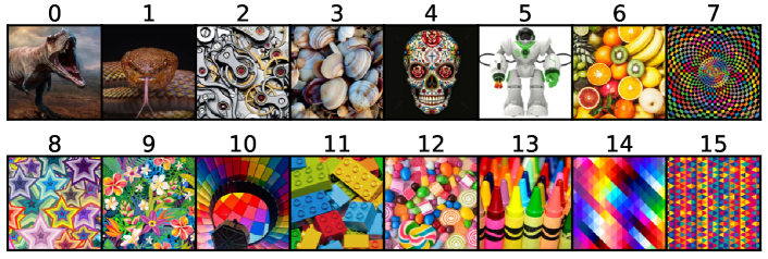
Figure 9: A list of Trojan-triggering images that we tried. The images are sorted by their training Trojan accuracy in ascending order. The last 5 images (11-15) were selected to be triggers for image-BI+ in our experiments.

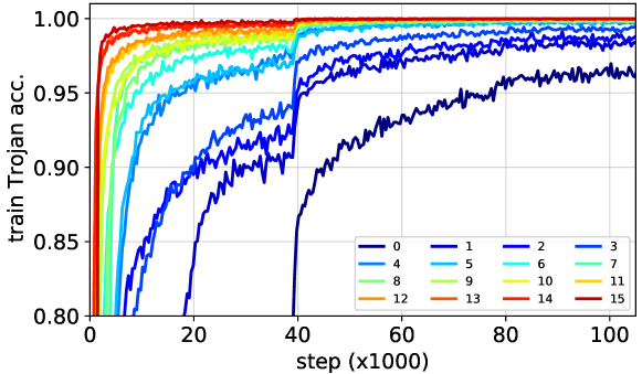
Figure 10: Training Trojan accuracy curves of BI on CIFAR10 w.r.t. different triggers in Fig. 9

0.C.1 BadNet+ and Noise/Image-BI+

BadNet+

BadNet+ is a variant of BadNet [11] that uses $M$ different image patches $p_{0},...,p_{M-1}$ ($p_{m}\in\mathbb{I}^{c\times h_{p}\times w_{p}}$, $0\leq m<M$) as Trojan triggers. Each patch $p_{m}$ is associated with a 2-tuple $l_{m}=(i,j)$ specifying the location of this patch in an input image, where $0\leq i<h-h_{p}$ and $0\leq j<w-w_{p}$. The pixel values and locations of the patches are generated randomly during construction. If not otherwise specified, we set $M=20$ and set the patch size $h_{p}\times w_{p}$ to be $5\times 5$ for MNIST, CIFAR10, GTSRB, and $8\times 8$ for CelebA.

Blended Injection+

Blended Injection+ (BI+) is similar to BadNet+ except that it uses full-size images $\rho_{0},...,\rho_{M-1}$ ($\rho_{m}\in\mathbb{I}^{c\times h\times w}$, $0\leq m<M$) as triggers instead of patches. Given a clean image $x$ and a Trojan-triggering image $\rho_{m}$, the corresponding Trojan image $\tilde{x}$ is computed as follows:

$$\tilde{x}=(1-\alpha)\cdot x+\alpha\cdot\rho_{m}$$

where $\alpha$ is the blending ratio set to 0.1 by default.

$\rho_{0},...,\rho_{M-1}$ can be either random noises or real images, resulting in two sub-versions of BI+, namely noise-BI+ and image-BI+. Choosing good Trojan-triggering images for image-BI+ is non-trivial. We tried various real images (Fig. 9) and found that they lead to very different attack success rates (aka Trojan accuracies) (Fig. 10). The best ones often contain colorful, repetitive patterns (e.g., “candies” or “crayons” images). Besides, we also observed that training image-BI+ with $M\geq 10$ is difficult since the classifier usually needs a lot of time to remember real images. Therefore, we selected only 5 images with the highest training Trojan accuracies (images 11-15 in Fig. 9) to be used as triggers for image-BI+ in our experiments.

noise-BI+, by contrast, achieves almost perfect Trojan accuracies even when $M$ is big ($M\approx 100$). We think the main reason behind this phenomenon is that a random noise image usually have much more distinct patterns than a real image. Although blending with clean input images may destroy some patterns in the noise image, many other patterns are still unaffected and can successfully cause the classifier to output the target class.

Dataset		Benign		BadNet+			noise-BI+			image-BI+			InpAwAtk			WaNet
		Clean		Clean	Trojan		Clean	Trojan		Clean	Trojan		Clean	Trojan		Clean	Trojan
MNIST		99.57		99.47	99.97		99.35	100.0		99.37	100.0		99.33	99.30		99.50	99.07
CIFAR10		94.71		94.83	100.0		94.57	100.0		95.13	99.90		94.57	99.40		94.27	99.67
GTSRB		99.63		99.42	100.0		99.45	100.0		99.34	100.0		98.97	99.66		99.16	99.42
CelebA		78.82		79.57	100.0		78.32	100.0		78.82	100.0		78.17	100.0		78.18	99.97

Table 12: Clean and Trojan accuracies of single-target attacks on the defense test set ($\mathcal{D}_{\text{test}}$) of different datasets.

Dataset		BadNet+			noise-BI+			image-BI+			InpAwAtk
		Clean	Trojan		Clean	Trojan		Clean	Trojan		Clean	Trojan
MNIST		99.37	98.54		99.57	99.38		99.53	99.25		99.23	97.64
CIFAR10		94.63	94.30		94.32	93.77		94.70	94.06		94.53	94.10
GTSRB		99.63	99.08		99.58	99.06		99.37	99.08		99.16	99.29

Table 13: Clean and Trojan accuracies of different all-target attacks on the defense test set ($\mathcal{D}_{\text{test}}$) of different datasets.

0.C.2 Results of Benchmark Attacks on $\mathcal{D}_{\text{test}}$

For completeness, we provide results of the benchmark attacks on $\mathcal{D}_{\text{test}}$ in Table 0.C.1 (for single-target mode) and in Table 0.C.1 (for all-target mode). The results in Table 0.C.1 are quite similar to the results on $\mathcal{D}_{\text{val}}\cup\mathcal{D}_{\text{test}}$ in Table 5.1. Since we were not successful in training the all-target version of WaNet, we exclude this attack from the results in Table 0.C.1.

Appendix 0.D Additional Results of Baseline Defenses

0.D.1 Network Pruning

Dataset		BadNet+				noise-BI+				image-BI+				InpAwAtk				WaNet
		1%	5%	10%		1%	5%	10%		1%	5%	10%		1%	5%	10%		1%	5%	10%
MNIST		37.38	22.73	14.98		14.21	11.00	6.75		14.69	6.31	4.72		3.32	3.32	3.32		1.18	1.18	1.18
CIFAR10		100.0	100.0	100.0		99.33	87.26	87.26		99.74	99.74	99.74		56.52	56.52	56.52		96.85	96.59	96.59
GTSRB		100.0	100.0	100.0		100.0	100.0	100.0		99.87	99.87	99.87		18.38	18.38	18.38		98.86	98.86	98.86
CelebA		84.08	63.35	50.64		100.0	99.97	99.97		99.87	99.87	99.80		100.0	100.0	99.97		98.22	88.48	53.10

Table 14: Trojan accuracies of $\mathtt{C}$ pruned by Network Pruning at 1%, 5%, and 10% decrease in clean accuracy. Smaller values are better. Results are computed on $\mathcal{D}^{\prime}_{\text{test}}$.

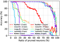
(a) MNIST

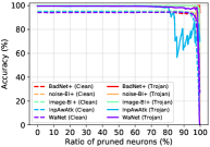
(b) CIFAR10

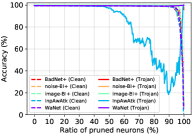
(c) GTSRB

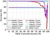
(d) CelebA

Figure 11: Clean accuracy (dashed) and Trojan accuracy (solid) curves of $\mathtt{C}$ pruned by Network Pruning for different attacks and datasets which correspond to the results in Table 0.D.1.

We provide the Trojan accuracies of Network Pruning (NP) [22] at 1%, 5%, and 10% decrease in clean accuracy in Table 0.D.1 and the corresponding pruning curves in Fig. 11. It is clear that NP is a very ineffective Trojan mitigation method since the classifier pruned by NP still achieves nearly 100% Trojan accuracies on CIFAR10, GTSRB, and CelebA even when experiencing about 10% decrease in clean accuracy.

0.D.2 STRIP

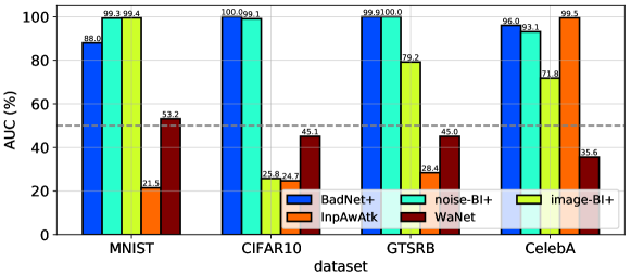
Figure 12: AUCs of STRIP against different attacks on different datasets. Larger values are better.

Dataset		BadNet+				noise-BI+				image-BI+				InpAwAtk				WaNet
		1%	5%	10%		1%	5%	10%		1%	5%	10%		1%	5%	10%		1%	5%	10%
MNIST		88.45	64.40	36.25		13.95	0.00	0.00		16.40	0.05	0.00		99.95	99.80	99.15		99.85	97.55	92.40
CIFAR10		0.00	0.00	0.00		10.35	2.35	0.95		99.45	97.30	95.75		99.55	97.90	96.20		100.0	99.25	96.90
GTSRB		1.05	0.20	0.00		0.00	0.00	0.00		79.20	58.30	44.75		99.85	98.80	97.15		99.50	96.00	91.65
CelebA		17.50	11.20	7.70		33.80	19.80	14.70		75.75	62.35	54.45		1.90	1.20	1.00		99.80	98.55	96.20

Table 15: False negative rates (FNRs) of STRIP at 1%, 5%, and 10% false positive rate (FPR) for different attacks and datasets. Smaller values are better.

	BadNet+	noise-BI+	image-BI+	InpAwAtk	WaNet
MNIST
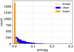
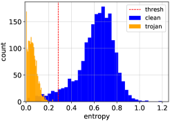
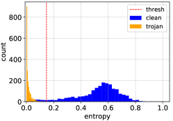
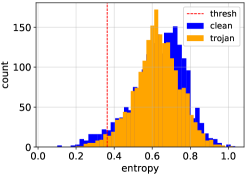
CIFAR10
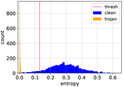
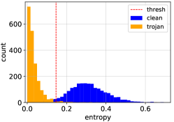
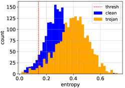
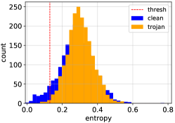
GTSRB
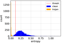
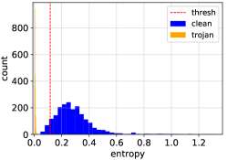
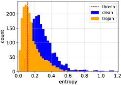
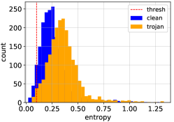
CelebA

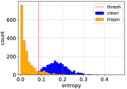
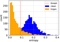
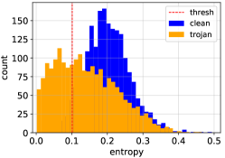
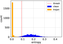
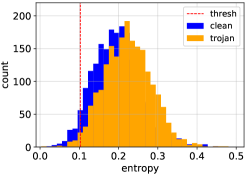
Figure 13: Histograms of entropies computed by STRIP for different attacks and datasets. The vertical red dashed line in each plot indicates the threshold at 5% false positive rate.

In Table 0.D.2, we report the false negative rates (FNRs) of STRIP at 1%, 5%, and 10% false positive rate (FPR). We also provide the AUCs and the entropy histograms of STRIP in Figs. 12 and 0.D.2, respectively. Note that AUCs are only suitable for experimental purpose not practical use since in real-world scenarios, we still have to compute thresholds based on FPRs on clean data. STRIP achieves very high FNRs on MNIST, CIFAR10, and GTSRB when defending against InpAwAtk and WaNet (Table 0.D.2) which corresponds to low AUCs (Fig. 12).

0.D.3 Neural Cleanse

Dataset		BadNet+				noise-BI+				image-BI+				InpAwAtk				WaNet
		1%	5%	10%		1%	5%	10%		1%	5%	10%		1%	5%	10%		1%	5%	10%
MNIST		0.00	0.00	0.00		0.00	0.00	0.00		0.00	0.00	0.00		0.00	0.00	0.00		-	-	-
CIFAR10		0.00	0.00	0.00		7.37	1.11	0.70		0.00	0.00	0.00		-	-	-		-	-	-
GTSRB		61.94	48.23	48.23		78.71	1.03	1.03		51.74	51.74	51.74		49.02	38.33	38.33		2.75	1.58	1.58
CelebA		75.97	26.73	7.63		99.95	98.75	95.30		99.75	96.21	83.62		99.87	98.42	93.31		-	-	-

Table 16: Trojan accuracies of the Trojan classifier $\mathtt{C}$ pruned by Neural Cleanse Pruning at 1%, 5%, and 10% decrease in clean accuracy for different attacks and datasets. Smaller values are better. Some results for InpAwAtk and WaNet are not available because Neural Cleanse fails to classify $\mathtt{C}$ as Trojan-infected in these cases (Fig. 4a).

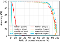
(a) MNIST

(b) CIFAR10

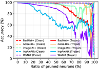
(c) GTSRB

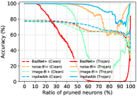
(d) CelebA

Figure 14: Clean accuracy (dashed) and Trojan accuracy (solid) curves of the Trojan classifier $\mathtt{C}$ pruned by Neural Cleanse Pruning for different attacks and datasets which correspond to the results in Table 0.D.3.

Dataset		BadNet+				noise-BI+				image-BI+				InpAwAtk				WaNet
		1%	5%	10%		1%	5%	10%		1%	5%	10%		1%	5%	10%		1%	5%	10%
MNIST		9.75	4.75	3.25		0.00	0.00	0.00		0.00	0.00	0.00		0.80	0.30	0.15		-	-	-
CIFAR10		99.50	78.90	0.65		90.55	39.30	0.05		95.50	56.90	0.40		-	-	-		-	-	-
GTSRB		100.0	0.40	0.00		0.00	0.00	0.00		0.03	0.00	0.00		99.48	92.17	86.65		3.02	0.40	0.32
CelebA		2.25	0.00	0.00		17.70	0.65	0.00		50.20	11.60	2.35		88.25	42.15	13.60		-	-	-

Table 17: False negative rates (FNRs) computed by Neural Cleanse Input Checking at 1%, 5%, and 10% false positive rate (FPR) for different attacks and datasets. Smaller values are better.

After classifying $\mathtt{C}$ as Trojan-infected, Neural Cleanse (NC) mitigates Trojans via pruning $\mathtt{C}$ or via input checking. We refer to these two methods as Neural Cleanse Pruning (NCP) and Neural Cleanse Input Checking (NCIC). Both methods build a set of synthetic Trojan images by blending all clean images in $\mathcal{D}_{\text{val}}$ with the synthetic trigger corresponding to the detected target class. NCP ranks neurons in the second last layer of $\mathtt{C}$ according to their average activation gaps computed on the synthetic Trojan images and the corresponding clean images in $\mathcal{D}_{\text{val}}$ in descending order. It gradually prunes the neurons with the highest ranks first until certain decrease in clean accuracy is met. NCIC, on the other hand, picks the top 1% of the neurons in the second last layer of $\mathtt{C}$ with largest average activations on the synthetic

Trojan images to form a characteristic group of Trojan neurons. Given an input image $x$, NCIC considers the mean activations of the neurons in the group w.r.t. $x$ as a score for detecting whether $x$ contains Trojan triggers or not. If the score is greater than a threshold, $x$ is considered as a Trojan image, otherwise, a clean image. The threshold is chosen based on the scores of all clean images in $\mathcal{D}_{\text{val}}$. We provide the results of NCP in Table 0.D.3, Fig. 14 and the results of NCIC in Table 0.D.3. At 5% decrease in clean accuracy, NCP reduces the Trojan accuracies of all the attacks except WaNet to almost 0% on MNIST and CIFAR10. However, NCP is ineffective against these attacks especially image-BI+ and InpAwAtk on GTSRB and CelebA. At 10% FPR, NCIC achieves nearly perfect FNRs against BadNet+, noise-BI+, and image-BI+ on all datasets but is also ineffective against InpAwAtk on GTSRB and CelebA. Note that both NCP and NCIC have almost no effect against WaNet on MNIST, CIFAR10, and CelebA since NC misclassifies the Trojan classifiers w.r.t. this attack as benign.

0.D.4 Februus

Figure 15: Examples of heatmaps computed by Februus’s GradCAM at different layers of $\mathtt{C}$ ordered from bottom (layer2.0.conv2) to top (layer4.1.conv2). The dataset is CIFAR10 and the classifier is a PreactResNet18 [15]. The Trojan attack is BadNet+. It is clear that only some layers give reasonably good results.

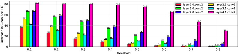
(a) Decrease in clean accuracy ($\downarrow$C)

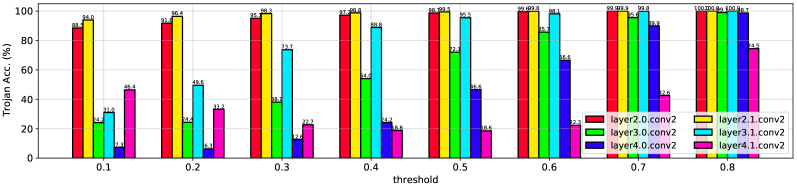
(b) Trojan accuracy (T)

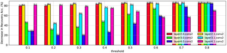
(c) Decrease in recovery accuracy ($\downarrow$R)

Figure 16: Decreases in clean accuracy (a), Trojan accuracies (b), and decreases in recovery accuracy (c) of Februus when mitigating BadNet+’s Trojans on CIFAR10 w.r.t. different heatmap layers and binary thresholds.

We reimplement Februus based on the official code provided by the authors. Since there is no script for training the inpainting GAN in the authors’ code, we use the “inpaint” function from OpenCV instead. Februus has 2 main hyperparameters that need to be tuned which are: i) the convolutional layer of $\mathtt{C}$ at which GradCAM computes heatmaps (“heatmap layer” for short) and ii) the threshold for converting GradCAM heatmaps into binary masks (“binary threshold” for short). As shown in Fig. 16, the performance of Februus greatly depends on these hyperparameters. Increasing the binary threshold means smaller areas are masked and inpainted, which usually leads to smaller decreases in clean accuracy (smaller $\downarrow$Cs) yet higher Trojan accuracies (higher Ts). Meanwhile, choosing top layers of $\mathtt{C}$ to compute heatmap (e.g., layer4) usually causes bigger $\downarrow$Cs yet lower Ts since the selected regions are often broader (Fig. 15). For simplicity, we choose the (layer, threshold) setting that gives the smallest decrease in recovery accuracy ($\downarrow$R) of Februus when defending against BadNet+ and apply this setting to all other attacks.

0.D.5 Neural Attention Distillation

We reimplement Neural Attention Distillation (NAD) based on the official code provided by the authors. We finetune the original Trojan classifier $\mathtt{C}$ to obtain the teacher $\mathtt{T}$ in 10 epochs. After that, we distill knowledge from $\mathtt{T}$ to $\mathtt{C}$ in 20 more epochs. In both cases, the batch size is 64 and the optimizer is Adam with an learning rate of 0.0001 divided by 10 after 10 epochs. We note that in the original paper, the authors reported that they used an initial learning rate of 0.1 and divided it by 10 after every 2 epochs during knowledge distillation. However, in our experiment, we found that such an initial learning rate is too large for distillation and can cause a significant drop in the clean accuracy of $\mathtt{C}$ which is hard to be recovered even if the learning rate is decayed later.

Appendix 0.E Additional Results and Ablation Studies of Our Defenses

Dataset	Defense	BadNet+			noise-BI+			image-BI+			InpAwAtk
		$\downarrow$C	T	$\downarrow$R	$\downarrow$C	T	$\downarrow$R	$\downarrow$C	T	$\downarrow$R	$\downarrow$C	T	$\downarrow$R
	IF	0.00	75.90	76.30	-0.03	99.30	99.47	0.13	6.96	6.96	0.00	95.74	96.17
MNIST	VIF	-0.07	49.67	50.17	-0.07	4.06	4.23	0.07	0.20	0.23	-0.23	63.58	64.21
	AIF	0.47	19.31	20.27	0.13	0.03	0.10	0.03	0.03	0.13	-0.13	23.90	24.53
	IF	3.93	1.57	8.03	2.63	1.17	3.30	3.60	18.90	22.20	3.83	9.97	14.63
CIFAR10	VIF	8.13	1.87	12.73	6.27	1.33	6.72	6.83	5.67	11.90	7.96	5.95	16.87
	AIF	5.67	1.23	9.13	4.40	0.97	5.47	5.13	5.10	9.63	5.43	6.73	14.33
	IF	0.29	0.11	1.58	0.13	0.21	1.18	-0.26	61.57	62.25	0.11	3.97	4.50
GTSRB	VIF	0.47	0.32	3.36	0.32	0.37	1.26	0.16	6.28	8.23	0.11	0.60	1.58
	AIF	0.11	0.29	2.08	-0.05	0.29	1.74	0.11	1.21	3.23	-0.16	2.02	2.39

Table 18: Decreases in clean accuracy ($\downarrow$Cs), Trojan accuracies (Ts), and recovery accuracies ($\downarrow$Rs) of our filtering defenses (IF, VIF, AIF) against different all-target Trojan attacks on different datasets. Smaller values are better. For a particular dataset, attack, and metric, the best defense is highlighted in bold.

Dataset	Defense	BadNet+		noise-BI+		image-BI+		InpAwAtk
		FPR	FNR	FPR	FNR	FPR	FNR	FPR	FNR
MNIST	IFtC	0.20	77.83	0.10	99.63	0.23	7.22	0.20	97.44
	VIFtC	0.20	49.97	0.07	4.19	0.07	0.27	0.33	64.85
	AIFtC	0.70	19.24	0.27	0.07	0.30	0.07	0.40	24.83
CIFAR10	IFtC	7.13	1.00	6.10	0.70	6.70	18.57	6.30	9.97
	VIFtC	12.10	1.30	10.14	1.12	10.50	5.40	11.13	5.83
	AIFtC	9.07	0.87	8.03	1.10	8.47	5.40	8.90	6.70
GTSRB	IFtC	0.50	0.08	0.29	0.29	0.42	62.57	0.34	3.97
	VIFtC	0.68	0.32	0.58	0.47	0.84	6.15	0.58	0.55
	AIFtC	0.34	0.42	0.26	0.26	0.79	0.92	0.45	2.05

Table 19: FPRs and FNRs of our FtC defenses against different all-target attacks. Smaller values are better. For a particular dataset, attack, and metric, the best defense is highlighted in bold.

0.E.1 Results of Our Defenses against All-target Attacks

In Tables 0.E and 19, we show the results our filtering and FtC defenses against different all-target attacks. On CIFAR10 and GTSRB, VIF/VIFtC and AIF/AIFtC are comparable. However, on MNIST, AIF/AIFtC is clearly better than VIF/VIFtC.

Dataset	Def.	BadNet+			noise-BI+			image-BI+			InpAwAtk			WaNet
		$\downarrow$C	T	$\downarrow$R	$\downarrow$C	T	$\downarrow$R	$\downarrow$C	T	$\downarrow$R	$\downarrow$C	T	$\downarrow$R	$\downarrow$C	T	$\downarrow$R
MNIST	IP	0.37	1.29	3.60	0.03	3.69	10.92	0.13	1.81	11.72	0.30	1.14	2.10	0.20	1.66	1.70
	IF	0.27	2.47	4.99	0.10	0.16	13.52	0.13	1.29	12.02	0.21	0.96	2.08	0.23	0.34	0.61
CIFAR10	IP	4.23	2.74	8.60	3.60	0.78	4.97	4.27	35.85	33.60	5.20	20.48	22.80	5.37	34.85	30.37
	IF	4.15	2.30	7.79	3.32	1.01	4.43	4.76	37.48	34.30	4.47	16.35	18.96	3.21	4.82	6.80
GTSRB	IP	0.18	0.00	2.79	0.24	0.00	1.76	0.37	52.61	52.37	0.42	2.06	3.76	10.73	62.33	61.33
	IF	0.13	0.00	2.55	0.13	0.03	1.52	0.37	52.27	51.95	0.03	0.66	3.60	0.08	9.83	9.62
CelebA	IP	2.83	9.98	4.23	2.73	25.57	14.72	2.43	73.63	35.82	2.31	15.09	7.81	2.28	76.49	36.76
	IF	4.21	8.62	4.75	2.57	13.83	6.00	2.25	59.39	27.94	2.86	11.95	6.07	2.43	15.21	4.75

Table 20: Trojan filtering results (in %) of Input Processing [25] and our Input Filtering. For a particular dataset, attack, and metric, the best among the 2 defenses are highlighted in bold. Results taken from Table 5.3 are shown in italic.

0.E.2 Comparison between Input Filtering and Input Processing [25]

In Fig. 0.E.1, we compare the performances of our Input Filtering (IF) and Input Processing (IP) against all the benchmark attacks on all the datasets. It is clear that IF outperforms IP in terms of Trojan accuracy in most cases, especially under InputAwAtk and WaNet. For example, IP achieves very high (poor) Trojan accuracies of 34.85%, 62.33%, and 76.49% against WaNet on CIFAR10, GTSRB, and CelebA, respectively while our IF achieves only 4.82%, 9.83%, and 15.21%. These results empirically verify the importance of the term $-\log p_{\mathtt{C}}(y|x^{\circ})$ in the loss of IF. This term ensures that the filtered output $x^{\circ}$computed by $\mathtt{F}$ cannot cause harm to $\mathtt{C}$ even when it look very similar to the original input $x$.

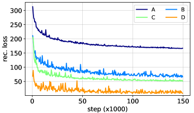
(a) Reconstruction losses

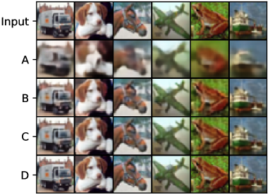
(b) Reconstructed images

Figure 17: Reconstruction losses (a) and reconstructed images (b) on CIFAR10 corresponding to the 4 autoencoders described in Table 0.B.2.

Arch.	BadNet+			noise-BI+			image-BI+			InpAwAtk			WaNet
	$\downarrow$C	T	$\downarrow$R	$\downarrow$C	T	$\downarrow$R	$\downarrow$C	T	$\downarrow$R	$\downarrow$C	T	$\downarrow$R	$\downarrow$C	T	$\downarrow$R
A	40.02	5.96	41.10	40.90	14.52	42.43	35.73	3.56	37.92	38.13	3.52	38.97	32.65	6.81	32.94
B	9.23	2.74	13.37	8.73	1.96	10.32	10.48	10.59	18.87	9.75	1.96	13.91	9.94	4.22	11.73
C	7.70	2.52	11.27	6.43	1.22	7.10	7.53	10.52	16.50	7.67	3.07	12.38	7.97	3.96	10.67
D	0.27	100.0	84.83	-0.02	100.0	84.57	0.21	99.81	84.96	-0.10	98.85	83.33	-0.07	98.96	83.35

Table 21: Trojan filtering results (in %) of VIF against different attacks on CIFAR10 w.r.t. different architectures of $\mathtt{F}$. For a particular dataset, attack, and metric, the best defense is highlighted in bold.

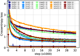
(a) Crossentropy loss

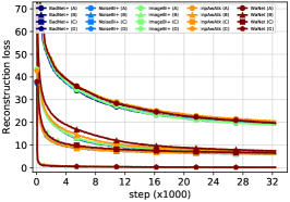
(b) Reconstruction loss

(c) KL divergence

Figure 18: Training curves of VIF against InpAwAtk on CIFAR10 ($\mathcal{D}_{\text{val}}$) w.r.t. the 4 architectures of $\mathtt{F}$ in Table 0.B.2.

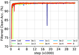
(a) Filtered Clean Acc.

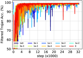
(b) Filtered Trojan Acc.

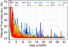
(c) Filtered Recovery Acc.

Figure 19: Test results of VIF using the architecture D (Table 0.B.2) for $\mathtt{F}$ against InpAwAtk on CIFAR10 ($\mathcal{D}_{\text{test}}$) w.r.t. different coefficient values for $D_{\text{KL}}$ ($\lambda_{2}$ in Eq. 3).

0.E.3 Different architectures of the filter $\mathtt{F}$

A major factor that affects the performance of $\mathtt{F}$ is its architecture. We consider an architecture of $\mathtt{F}$ to be more complex than others if $\mathtt{F}$ achieves smaller reconstruction loss on $\mathcal{D}_{\text{val}}$ with this architecture. In Section 4, we argued that an optimal filter should be neither too simple nor too complex. Here, we empirically verify this intuition by examining 4 different architectures of $\mathtt{F}$ for CIFAR10 marked as A, B, C, D (Table 0.B.2). Their complexities are greater in alphabetical order as shown in Figs. 17a, 17b. The architecture D has skip-connections between its encoder and decoder while A, B, C do not.

Denote $\mathtt{F}$ with the architectures A, B, C, D as $\mathtt{F}_{\text{A}}$, $\mathtt{F}_{\text{B}}$, $\mathtt{F}_{\text{C}}$, $\mathtt{F}_{\text{D}}$ respectively. As shown in Table 0.E.2, $\mathtt{F}_{\text{C}}$ is the best in terms of recovery accuracy although C is neither the simplest (A) nor the most complex architecture (D). $\mathtt{F}_{\text{A}}$ achieves reasonably low Trojan accuracies comparable to those of $\mathtt{F}_{\text{B}}$ and $\mathtt{F}_{\text{C}}$ but the worst clean accuracies. $\mathtt{F}_{\text{D}}$, by contrast, experiences almost no decrease in clean accuracy but achieves very high Trojan accuracies. The reason is that $\mathtt{F}_{\text{D}}$ simply copies all information from an input to the output via its skip-connections rather than learning compressed latent representations of input images. One can verify this by observing that the $D_{\text{KL}}$ (Eq. 3) of $\mathtt{F}_{\text{D}}$ is almost 0 (Fig. 18c). In this case, changing $\lambda_{2}$ has no effect on the Trojan accuracy of $\mathtt{F}_{\text{D}}$ as shown in Fig. 19. However, it is still possible to lower the Trojan accuracy of $\mathtt{F}_{\text{D}}$ without removing the skip-connections in D. For example, we can treat the latent representations corresponding to the skip-connections as random variables and apply the $D_{\text{KL}}$ to these variables like what we do with the middle representation. Or we can compress the whole $\mathtt{F}_{\text{D}}$ by using advanced network compression techniques [30, 27, 1]. These ideas are out of scope of this paper so we leave them for future work.

0.E.4 Explicit Normalization of Triggers in AIF

0.E.4.1 Theoretical Derivation

During training AIF, we observed that under the influence of $\mathcal{L}_{\text{VIF-gen}}$ (Eq. 8), the norm $\|m\|$ of a synthetic trigger mask $m$ usually increases overtime despite the fact that $\mathcal{L}_{\text{VIF-gen}}$ also contains a norm regularization term. The reason is that $\mathtt{G}$ is encouraged to output bigger Trojan triggers to fool $\mathtt{F}$. However, too big trigger causes the generated Trojan image $\tilde{x}$ to be very different from the input image $x$, which affects the learning of $\mathtt{F}$. One way to deal with this problem is explicitly normalizing $m$ so that its norm is always upper-bounded by $\delta$. Denoted by $\bar{m}$ the $\delta$-normalized version of $m$. $\bar{m}$ can be computed as follows:

$$\bar{m}=\begin{cases}m&\text{if}\ \|m\|\leq\delta\\ \delta\frac{m}{\|m\|}&\text{if}\ \|m\|>\delta\end{cases}$$ (11)

or more compactly,

$$\bar{m} =m\times\left(1-\frac{\max(\|m\|-\delta,0)}{\|m\|}\right)$$

$$=m\times\left(1-\frac{\text{ReLU}(\|m\|-\delta)}{\|m\|}\right)$$ (12)

In case the norm is L2, the second expression in Eq. 11 can be seen as the projection of $m$ onto the surface of a sphere of radius $\delta$. By replacing $\text{ReLU}(\cdot)$ in Eq. 12 with $\text{Softplus}(\cdot)$, we obtain a soft version of $\bar{m}$:

$$\bar{m}_{s} =m\times\left(1-\frac{\text{Softplus}(\|m\|-\delta,\tau)}{\|m\|}\right)$$

$$=m\times\left(1-\frac{\tau\log(1+\exp((\|m\|-\delta)/\tau))}{\|m\|}\right)$$ (13)

where $\tau>0$ is a temperature. $\bar{m}_{s}$ with smaller $\tau$ approximates $\bar{m}$ better. Generally, using $\bar{m}_{s}$ gives better gradient update than using $\bar{m}$. However, since Softplus is an upper-bound of ReLU, $\text{Softplus}(\|m\|-\delta,\tau)$ can be greater than $\|m\|$, which causes $\bar{m}_{s}$ to be negative. To avoid that, we slightly modify Eq. 13 into the equation below:

$$\bar{m}_{s}=m\times\left(1-\frac{\tau\log(1+\exp((\|m\|-\delta)/\tau))}{\|m\|+\Omega}\right)$$ (14)

where $\Omega>0$ is an added term to ensure that $\bar{m}_{s}\geq 0$. $\Omega$ can be computed from $\tau$ and $\delta$ by solving the following inequality:

$$\tau\log(1+\exp((\|m\|-\delta)/\tau))\leq\|m\|+\Omega$$

$$\Leftrightarrow 1+\exp\left(\frac{\|m\|-\delta}{\tau}\right)\leq\exp\left(\frac{\|m\|+\Omega}{\tau}\right)$$

$$\Leftrightarrow 1\leq\exp\left(\frac{\|m\|}{\tau}\right)\left(\exp\frac{\Omega}{\tau}-\exp\left(\frac{-\delta}{\tau}\right)\right)$$

$$\Leftrightarrow \exp\left(\frac{-\|m\|}{\tau}\right)\leq\exp\frac{\Omega}{\tau}-\exp\left(\frac{-\delta}{\tau}\right)$$

Since $\exp\left(\frac{-\|m\|}{\tau}\right)$ is always smaller than 1, we can choose $\Omega$ so that:

$$\exp\frac{\Omega}{\tau}-\exp\left(\frac{-\delta}{\tau}\right)=1$$

$$\Leftrightarrow \Omega=\tau\log\left(1+\exp\left(\frac{-\delta}{\tau}\right)\right)$$

In our experiments, we set $\delta=0.05$ and $\tau=0.01$. We also observed that the hard normalization (Eq. 12) and the soft normalization (Eq. 14) of $m$ give roughly the same performance.

Dataset	Norm.	BadNet+			noise-BI+			image-BI+			InpAwAtk			WaNet
		$\downarrow$C	T	$\downarrow$R	$\downarrow$C	T	$\downarrow$R	$\downarrow$C	T	$\downarrow$R	$\downarrow$C	T	$\downarrow$R	$\downarrow$C	T	$\downarrow$R
CIFAR10	w/	5.60	2.37	9.03	4.87	1.14	6.02	5.23	1.96	7.10	5.28	5.30	11.87	4.30	1.22	5.67
	wo/	5.90	2.15	10.00	5.60	0.78	7.50	6.60	1.56	7.53	6.20	2.56	9.37	5.80	2.22	8.10
GTSRB	w/	-0.16	0.00	1.87	0.05	0.00	0.81	0.13	7.47	9.54	-0.03	0.05	1.37	-0.05	0.50	0.42
	wo/	0.13	0.08	3.18	0.24	0.00	1.26	0.45	0.92	5.44	0.45	0.00	2.60	0.21	0.11	0.45

Table 22: Trojan filtering results (in %) of AIF with and without explicit trigger normalization against different attacks on CIFAR10 and GTSRB. For a particular attack, dataset and metric, the best result is highlighted in bold. Results taken from Table 5.3 are shown in italic.

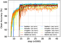
(a) Clean Accuracy

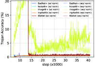
(b) Trojan Accuracy

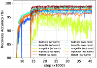
(c) Recovery Accuracy

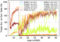
(d) Trojan Acc. on Sync. Data

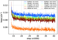
(e) $\log p(y|x^{\circ})$ ($\mathtt{F}$)

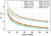
(f) $\|x^{\circ}-x\|$ ($\mathtt{F}$)

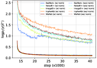
(g) $\log p(y|\tilde{x}^{\circ})$ ($\mathtt{F}$)

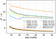
(h) $\|\tilde{x}^{\circ}-x\|$ ($\mathtt{F}$)

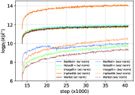
(i) $\log p(k|\tilde{x}^{\circ})$ ($\mathtt{G}$)

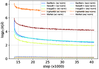
(j) $\log p(k|\tilde{x})$ ($\mathtt{G}$)

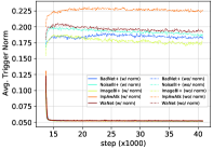
(k) $\|m\|$ ($\mathtt{G}$)

Figure 20: Test result curves and training loss curves of $\mathtt{F}$, $\mathtt{G}$ of VIF with and without explicit trigger normalization against different attacks on GTSRB. These plots correspond to the results in the bottom 2 rows in Table 0.E.4.1.

0.E.4.2 Empirical Results

From Table 0.E.4.1, we see that AIF with explicit trigger normalization (denoted as AIF-w) always achieve smaller $\downarrow$Cs and sometimes achieve larger Ts than the counterpart without explicit trigger normalization (denoted as AIF-wo). In general, AIF-w usually achieves lower $\downarrow$Rs than AIF-wo and is considered to be better so we set it as default. Fig. 20 provides a deeper insight into the results in Table 0.E.4.1. Without explicit trigger normalization, the generator $\mathtt{G}$ can easily fool $\mathtt{F}$ (low crossentropy losses in Fig. 20i) by just increasing the norm of the synthetic triggers (Fig. 20k). This makes $\tilde{x}$ more different from $x$ and causes more difficulty for $\mathtt{F}$ to force $\tilde{x}^{\circ}$ close to $x$ (Fig. 20h) as well as correcting the label of $\tilde{x}$ (Fig. 20g). The large difference between $\tilde{x}$ and $x$ also negatively affects the performance of $\mathtt{F}$ on reconstructing clean images (Fig. 20f). As a result, AIF-wo achieves much poorer Ts on synthetic Trojan images (Fig. 20d) than AIF-w. On ground-truth Trojan images, AIF-wo performs as well as AIF-w in terms of T (Fig. 20b) and worse than AIF-w in terms of $\downarrow$C (Fig. 20a) and $\downarrow$R (Fig. 20d).

Appendix 0.F Qualitative Results of Our Defenses

0.F.1 Against Benchmark Attacks

In Figs. 21a, 22a, 23a, 24a, we show some ground-truth (GT) Trojan images $\tilde{x}$ and their filtered counterparts $\tilde{x}^{\circ}$ computed by Februus (Feb.) and our filtering defenses (VIF, AIF) for different Trojan attacks and datasets. We also show the corresponding “counter-triggers” of $\tilde{x}^{\circ}$ defined as $|\tilde{x}^{\circ}-\tilde{x}|$ in Figs. 21b, 22b, 23b, 24b in comparison with the ground-truth Trojan triggers $|\tilde{x}-x|$. It is apparent that VIF and AIF correctly filter the true triggers of all the attacks without knowing them while Februus fails to filter the true triggers of noise-BI+, image-BI+, InpAwAtk and WaNet. The failure of Februus comes from the fact that GradCAM is unable to find regions containing full-sized, distributed triggers of noise/image-BI+ or isomorphic, input-specific triggers of InpAwAtk/WaNet. For BadNet+ and InpAwAtk, our filtering defenses mainly blur the triggers of these attacks instead of completely removing the triggers but this is enough to deactivate the triggers.

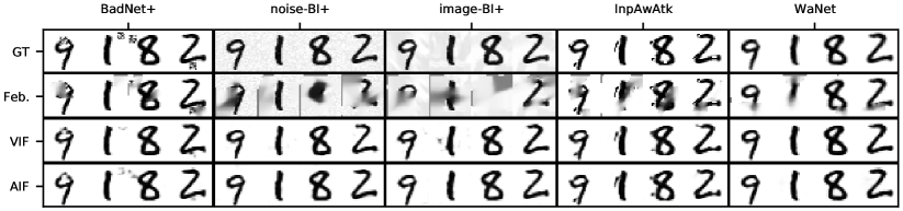
(a) Filtered images

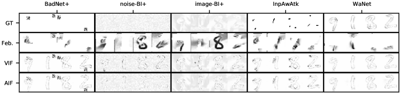
(b) Counter-triggers

Figure 21: (a): Ground-truth (GT) Trojan images of different attacks and the corresponding filtered images computed by Februus (Feb.), VIF, and AIF on MNIST. (b): GT triggers and counter-triggers w.r.t. the filtered images in (a).

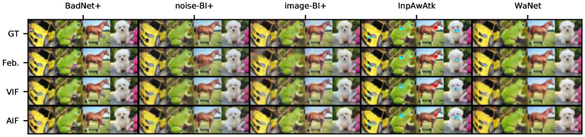
(a) Filtered images

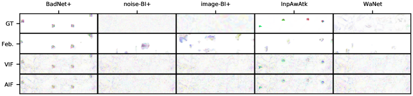
(b) Counter-triggers

Figure 22: (a): Ground-truth (GT) Trojan images of different attacks and the corresponding filtered images computed by Februus (Feb.), VIF, and AIF on CIFAR10. (b): GT triggers and counter-triggers w.r.t. the filtered images in (a).

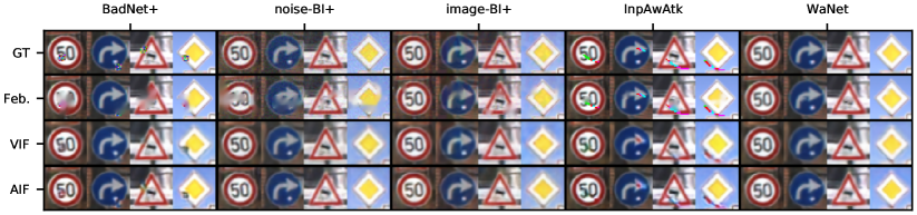
(a) Filtered images

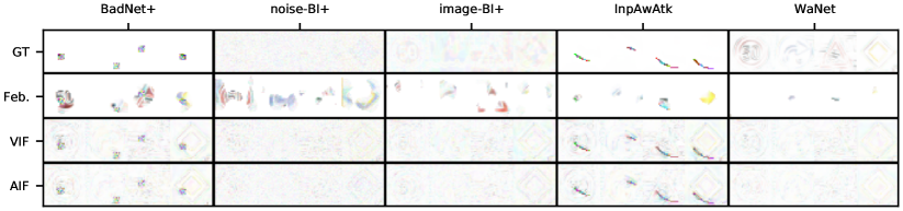
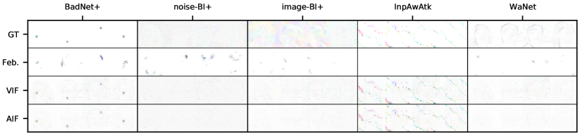
(b) Counter-triggers

Figure 23: (a): Ground-truth (GT) Trojan images of different attacks and the corresponding filtered images computed by Februus (Feb.), VIF, and AIF on GTSRB. (b): GT triggers and counter-triggers w.r.t. the filtered images in (a).

(a) Filtered images

(b) Counter-triggers

Figure 24: (a): Ground-truth (GT) Trojan images of different attacks and the corresponding filtered images computed by Februus (Feb.), VIF, and AIF on CelebA. (b): GT triggers and counter-triggers w.r.t. the filtered images in (a).

0.F.2 Against Attacks with Large-Norm Triggers

In Fig. 25, we visualize the filtered images and their corresponding counter-triggers computed by our methods for Trojan images of BadNet+ with different trigger sizes and of noise-BI+ with different blending ratios. In general, our filtering defenses can effectively deactivate triggers embedded in the Trojan images via modifying the trigger pixels but cannot fully reconstruct the original clean images. These qualitative results correspond to the quantitative results in Tables 5.4.3, 5.4.3.

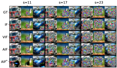
(a) Filtered images (BadNet+)

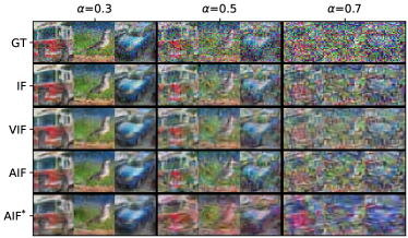
(b) Filtered images (noise-BI+)

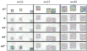
(c) Counter-triggers (BadNet+)

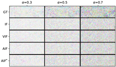
(d) Counter-triggers (noise-BI+)

Figure 25: (a)/(b): Ground-truth (GT) Trojan images of BadNet+/noise-BI+ and the corresponding filtered images computed by IF, VIF, AIF, and AIF without explicit trigger normalization (AIF^∗). (c)/(d): GT triggers and counter-triggers w.r.t. the filtered images in (a)/(b).

References

- [1] van Baalen, M., Louizos, C., Nagel, M., Amjad, R.A., Wang, Y., Blankevoort, T., Welling, M.: Bayesian bits: Unifying quantization and pruning. arXiv preprint arXiv:2005.07093 (2020)
- [2] Chen, B., Carvalho, W., Baracaldo, N., Ludwig, H., Edwards, B., Lee, T., Molloy, I., Srivastava, B.: Detecting backdoor attacks on deep neural networks by activation clustering. arXiv preprint arXiv:1811.03728 (2018)
- [3] Chen, H., Fu, C., Zhao, J., Koushanfar, F.: DeepInspect: A Black-box Trojan Detection and Mitigation Framework for Deep Neural Networks. In: Proceedings of the 28th International Joint Conference on Artificial Intelligence. AAAI Press. pp. 4658–4664 (2019)
- [4] Chen, X., Liu, C., Li, B., Lu, K., Song, D.: Targeted backdoor attacks on deep learning systems using data poisoning. arXiv preprint arXiv:1712.05526 (2017)
- [5] Doan, B.G., Abbasnejad, E., Ranasinghe, D.C.: Februus: Input purification defense against trojan attacks on deep neural network systems. In: Annual Computer Security Applications Conference. pp. 897–912 (2020)
- [6] Dong, Y., Yang, X., Deng, Z., Pang, T., Xiao, Z., Su, H., Zhu, J.: Black-box detection of backdoor attacks with limited information and data. arXiv preprint arXiv:2103.13127 (2021)
- [7] Fawzi, A., Fawzi, H., Fawzi, O.: Adversarial vulnerability for any classifier. arXiv preprint arXiv:1802.08686 (2018)
- [8] Gao, Y., Xu, C., Wang, D., Chen, S., Ranasinghe, D.C., Nepal, S.: Strip: A Defence Against Trojan Attacks on Deep Neural Networks. In: Proceedings of the 35th Annual Computer Security Applications Conference. pp. 113–125 (2019)
- [9] Goodfellow, I., Pouget-Abadie, J., Mirza, M., Xu, B., Warde-Farley, D., Ozair, S., Courville, A., Bengio, Y.: Generative adversarial nets. Advances in neural information processing systems 27 (2014)
- [10] Goodfellow, I.J., Shlens, J., Szegedy, C.: Explaining and harnessing adversarial examples. arXiv preprint arXiv:1412.6572 (2014)
- [11] Gu, T., Dolan-Gavitt, B., Garg, S.: Badnets: Identifying vulnerabilities in the machine learning model supply chain. arXiv preprint arXiv:1708.06733 (2017)
- [12] Guo, W., Wang, L., Xing, X., Du, M., Song, D.: Tabor: A highly accurate approach to inspecting and restoring trojan backdoors in ai systems. arXiv preprint arXiv:1908.01763 (2019)
- [13] Harikumar, H., Le, V., Rana, S., Bhattacharya, S., Gupta, S., Venkatesh, S.: Scalable backdoor detection in neural networks. In: Joint European Conference on Machine Learning and Knowledge Discovery in Databases (ECML PKDD). pp. 289–304. Springer (2020)
- [14] He, K., Zhang, X., Ren, S., Sun, J.: Deep residual learning for image recognition. In: Proceedings of the IEEE conference on computer vision and pattern recognition. pp. 770–778 (2016)
- [15] He, K., Zhang, X., Ren, S., Sun, J.: Identity mappings in deep residual networks. In: European conference on computer vision. pp. 630–645. Springer (2016)
- [16] Ji, Y., Zhang, X., Wang, T.: Backdoor attacks against learning systems. In: IEEE Conference on Communications and Network Security. pp. 1–9. IEEE (2017)
- [17] Kingma, D.P., Ba, J.: Adam: A Method for Stochastic Optimization. arXiv preprint arXiv:1412.6980 (2014)
- [18] Kingma, D.P., Welling, M.: Auto-encoding variational bayes. arXiv preprint arXiv:1312.6114 (2013)
- [19] Krizhevsky, A.: Learning Multiple Layers of Features from Tiny Images. Tech. rep. (2009)
- [20] Li, Y., Lyu, X., Koren, N., Lyu, L., Li, B., Ma, X.: Neural attention distillation: Erasing backdoor triggers from deep neural networks. arXiv preprint arXiv:2101.05930 (2021)
- [21] Li, Y., Li, Y., Wu, B., Li, L., He, R., Lyu, S.: Backdoor attack with sample-specific triggers. arXiv preprint arXiv:2012.03816 (2020)
- [22] Liu, K., Dolan-Gavitt, B., Garg, S.: Fine-pruning: Defending against backdooring attacks on deep neural networks. In: International Symposium on Research in Attacks, Intrusions, and Defenses. pp. 273–294. Springer (2018)
- [23] Liu, Y., Lee, W.C., Tao, G., Ma, S., Aafer, Y., Zhang, X.: ABS: Scanning Neural Networks for Back-doors by Artificial Brain Stimulation. In: Proceedings of the ACM SIGSAC Conference on Computer and Communications Security. pp. 1265–1282 (2019)
- [24] Liu, Y., Ma, X., Bailey, J., Lu, F.: Reflection backdoor: A natural backdoor attack on deep neural networks. In: European Conference on Computer Vision. pp. 182–199. Springer (2020)
- [25] Liu, Y., Xie, Y., Srivastava, A.: Neural trojans. In: 2017 IEEE International Conference on Computer Design (ICCD). pp. 45–48. IEEE (2017)
- [26] Liu, Z., Luo, P., Wang, X., Tang, X.: Deep learning face attributes in the wild. In: Proceedings of the IEEE international conference on computer vision. pp. 3730–3738 (2015)
- [27] Louizos, C., Ullrich, K., Welling, M.: Bayesian compression for deep learning. arXiv preprint arXiv:1705.08665 (2017)
- [28] Madry, A., Makelov, A., Schmidt, L., Tsipras, D., Vladu, A.: Towards deep learning models resistant to adversarial attacks. arXiv preprint arXiv:1706.06083 (2017)
- [29] Moeskops, P., Veta, M., Lafarge, M.W., Eppenhof, K.A., Pluim, J.P.: Adversarial training and dilated convolutions for brain mri segmentation. In: Deep learning in medical image analysis and multimodal learning for clinical decision support, pp. 56–64. Springer (2017)
- [30] Molchanov, D., Ashukha, A., Vetrov, D.: Variational dropout sparsifies deep neural networks. In: International Conference on Machine Learning. pp. 2498–2507. PMLR (2017)
- [31] Muñoz-González, L., Pfitzner, B., Russo, M., Carnerero-Cano, J., Lupu, E.C.: Poisoning attacks with generative adversarial nets. arXiv preprint arXiv:1906.07773 (2019)
- [32] Nguyen, A., Tran, A.: Input-aware dynamic backdoor attack. arXiv preprint arXiv:2010.08138 (2020)
- [33] Nguyen, A., Tran, A.: Wanet–imperceptible warping-based backdoor attack. International Conference on Learning Representations (2021)
- [34] Parkhi, O.M., Vedaldi, A., Zisserman, A.: Deep face recognition (2015)
- [35] Qiao, X., Yang, Y., Li, H.: Defending neural backdoors via generative distribution modeling. arXiv preprint arXiv:1910.04749 (2019)
- [36] Redmon, J., Divvala, S., Girshick, R., Farhadi, A.: You only look once: Unified, real-time object detection. In: Proceedings of the IEEE conference on computer vision and pattern recognition. pp. 779–788 (2016)
- [37] Saha, A., Subramanya, A., Pirsiavash, H.: Hidden trigger backdoor attacks. In: Proceedings of the AAAI Conference on Artificial Intelligence. vol. 34, pp. 11957–11965 (2020)
- [38] Salem, A., Wen, R., Backes, M., Ma, S., Zhang, Y.: Dynamic backdoor attacks against machine learning models. arXiv preprint arXiv:2003.03675 (2020)
- [39] Schroff, F., Kalenichenko, D., Philbin, J.: Facenet: A unified embedding for face recognition and clustering. In: Proceedings of the IEEE conference on computer vision and pattern recognition. pp. 815–823 (2015)
- [40] Selvaraju, R.R., Cogswell, M., Das, A., Vedantam, R., Parikh, D., Batra, D.: Grad-cam: Visual explanations from deep networks via gradient-based localization. In: Proceedings of the IEEE international conference on computer vision. pp. 618–626 (2017)
- [41] Shafahi, A., Huang, W.R., Najibi, M., Suciu, O., Studer, C., Dumitras, T., Goldstein, T.: Poison frogs! targeted clean-label poisoning attacks on neural networks. arXiv preprint arXiv:1804.00792 (2018)
- [42] Stallkamp, J., Schlipsing, M., Salmen, J., Igel, C.: Man vs. Computer: Benchmarking Machine Learning Algorithms for Traffic Sign Recognition. Neural Networks pp. 323–332 (2012)
- [43] Sultani, W., Chen, C., Shah, M.: Real-world anomaly detection in surveillance videos. In: Proceedings of the IEEE conference on computer vision and pattern recognition. pp. 6479–6488 (2018)
- [44] Thys, S., Van Ranst, W., Goedemé, T.: Fooling automated surveillance cameras: adversarial patches to attack person detection. In: Proceedings of the IEEE/CVF Conference on Computer Vision and Pattern Recognition Workshops. pp. 0–0 (2019)
- [45] Tran, B., Li, J., Madry, A.: Spectral Signatures in Backdoor Attacks. In: Advances in Neural Information Processing Systems. pp. 8000–8010 (2018)
- [46] Vincent, P., Larochelle, H., Bengio, Y., Manzagol, P.A.: Extracting and composing robust features with denoising autoencoders. In: Proceedings of the 25th international conference on Machine learning. pp. 1096–1103 (2008)
- [47] Wang, B., Yao, Y., Shan, S., Li, H., Viswanath, B., Zheng, H., Zhao, B.Y.: Neural Cleanse: Identifying and Mitigating Backdoor Attacks in Neural Networks. In: IEEE Symposium on Security and Privacy. pp. 707–723. IEEE (2019)
- [48] Wang, R., Zhang, G., Liu, S., Chen, P.Y., Xiong, J., Wang, M.: Practical detection of trojan neural networks: Data-limited and data-free cases. In: Computer Vision–ECCV 2020: 16th European Conference, Glasgow, UK, August 23–28, 2020, Proceedings, Part XXIII 16. pp. 222–238. Springer (2020)
- [49] Wenger, E., Passananti, J., Bhagoji, A.N., Yao, Y., Zheng, H., Zhao, B.Y.: Backdoor attacks against deep learning systems in the physical world. In: Proceedings of the IEEE/CVF Conference on Computer Vision and Pattern Recognition. pp. 6206–6215 (2021)
- [50] Wu, D., Wang, Y.: Adversarial neuron pruning purifies backdoored deep models. Advances in Neural Information Processing Systems 34 (2021)
- [51] Yang, D., Xu, D., Zhou, S.K., Georgescu, B., Chen, M., Grbic, S., Metaxas, D., Comaniciu, D.: Automatic liver segmentation using an adversarial image-to-image network. In: International Conference on Medical Image Computing and Computer-Assisted Intervention. pp. 507–515. Springer (2017)
- [52] Zagoruyko, S., Komodakis, N.: Paying more attention to attention: Improving the performance of convolutional neural networks via attention transfer. arXiv preprint arXiv:1612.03928 (2016)
- [53] Zhao, P., Chen, P.Y., Das, P., Ramamurthy, K.N., Lin, X.: Bridging mode connectivity in loss landscapes and adversarial robustness. arXiv preprint arXiv:2005.00060 (2020)
- [54] Zhao, S., Song, J., Ermon, S.: Infovae: Information maximizing variational autoencoders. arXiv preprint arXiv:1706.02262 (2017)
- [55] Zhu, C., Huang, W.R., Li, H., Taylor, G., Studer, C., Goldstein, T.: Transferable clean-label poisoning attacks on deep neural nets. In: International Conference on Machine Learning. pp. 7614–7623. PMLR (2019)