Acknowledgements

First of all, I want to express my deepest gratitude to Vincent Vennin who gave me the opportunity to conduct research in a motivating and pleasant environment within the Laboratoire AstroParticule et Cosmologie (APC). As a PhD advisor, he introduced me to the field of early universe cosmology and gave me motivations to contuct research on the field of primordial black holes. I want to thank him as well for his psychological support and encouragement to endure and continue the journey towards the PhD.

In addition, I am delighted to thank my collaborators David Langlois, Jérôme Martin and Lucas Pinol with I whom I worked closely. I learnt a lot from their pedagogy, scientific rigour, physical intuitiveness and scientific integrity.

A special thankfulness goes to Ilia Musco, with whom I collaborated a lot on the field of the gravitational collapse of primordial black holes. I want to thank him together with Antonio Riotto for the kind hospitality in the Departement of Theoretical Physics of the University of Geneva as well as for the fruitful scientific discussions we had from which I learnt a lot.

I want to thank as well Sébastien Clesse, Chris Thomas Byrnes, Antonio Riotto and Danièle Steer for their scientific interest to my work and for having accepted being members of my PhD thesis jury and review my PhD manuscript.

Furthermore, I want to thank the directors of APC, Stavros Katsanevas and Antoine Kouchner and the director of the theory group of APC Dimitri Semikoz for providing me with the best conditions in order to carry out research as well as the directors of the STEP’UP Doctoral School Yannick Giraud-Héraud and Alessandra Tonazzo for their patience and for their guidance to find the necessary funding resources for my PhD.

At this point, I have to acknowledge thankfulness to the Fondation CFM pour la Recherche in France, the Alexander S. Onassis Public Benefit Foundation in Greece, the Foundation for Education and European Culture in Greece and the A.G. Leventis Foundation for their interest to my PhD research field as well as for their funding support during the three years of my PhD studies.

Moreover, it’s a pleasure to give a special thanks to my office mates Célia, Gabriel, Jan and Amélie who contributed to forming a nice working environment for me as well as to my PhD colleagues in APC Pierre, Jewel and Hugo for the nice discussions we had during launch and coffee times.

In addition, I am grateful to my spiritual fathers, archimandrite father Gabriel, archpriest father Panagiotis and the Bishop Irénée of Reggio for their psychological support and kindness as well as for providing me with all the necessary spiritual arms during my PhD studies.

Last but not least, I want to thank my parents Nikolaos and Regina, my brother Christos and my fiancée Adela-Maria for their love, patience and support during these years and all the upcoming ones.

Abstract

This thesis by publication is devoted to the study of aspects of the early universe in the context of primordial black hole (PBH) physics. Since the early ’70s, when PBHs were initially proposed, PBHs have been attracting an increasing interest within the scientific community given the fact that they can address a number of fundamental issues of modern cosmology and at the same time give access to different physical phenomena depending on their mass. Interestingly, with low mass PBHs one can probe and constrain the physics of the early universe, such as inflation and reheating whereas with high mass PBHs one can probe gravitational physics phenomena like the large-scale structure formation and the origin of dark matter.

In the following PhD thesis, we firstly review the fundamentals of the early universe cosmology and we recap the basics of the PBHs physics covering both theoretical and observational aspects. In particular, we propose a refinement in the determination of the PBH formation threshold, a fundamental quantity in PBH physics, in the context of a time-dependent equation-of-state parameter. Afterwards, we briefly present the theory of inflationary perturbations, which is the theoretical framework within which PBHs are studied in this thesis.

Then, in the second part of the thesis, we review the core of the research conducted within my PhD, in which aspects of the early universe and the gravitational wave physics are combined with the physics of PBHs. Moreover, aspects of the PBH gravitational collapse process are studied in the presence of anisotropies. Specifically, we study PBHs produced from the preheating instability in the context of single-field inflation. In particular, we find that PBHs produced during preheating can potentially dominate the universe’s content and drive reheating through their evaporation. Then, we focus on the scalar induced second-order stochastic gravitational wave background (SGWB) produced during an era before BBN in which ultralight PBHs dominate the energy budget of the universe. By taking then into account gravitational wave backreaction effects we set model-independent constraints on the initial abundance of ultralight PBHs as a function of their mass. Afterwards, we study in a covariant way the anisotropic spherical gravitational collapse of PBHs during a radiation-dominated era in which one can compute the PBH formation threshold as a function of the anisotropy.

Finally, we summarize our research results by discussing future prospects opened up as a result of the work we have done within the PhD. In particular, we emphasize the fact that one can narrow down the CMB observational predictions by studying PBHs produced from the single-field inflation preheating instability as well as the potential detectability of ultralight PBHs by future gravitational experiments such as LISA, Einstein Telescope and SKA.

Keywords: primordial black holes, inflation, preheating, induced gravitational waves, primordial black hole gravitational collapse

Résumé

Cette thèse sur articles est dédiée à l’étude des aspects de l’univers primordial par le biais des trous noirs primordiaux (TNP). Depuis que les TNP ont été initialement proposés dans les années 70, ils attirent de plus en plus l’intérêt de la communauté scientifique étant donné le fait que ces objets astrophysiques apportent un éclairage sur un grand nombre de problèmes de la cosmologie contemporaine et en parallèle peuvent donner accès à une grande variété de phénomènes physiques en fonction de de leur masse. En particulier, les TNP de petite masse peuvent donner accès à la physique de l’univers primordial comme la physique de l’inflation et du rechauffement tandis qu’ avec les TNP de grande masse on peut explorer des phénomènes de la physique gravitationnelle comme la formation des structures de grande échelle et l’origine de la matière noire.

Dans cette thèse, on rapelle tout d’abord les fondements de la cosmologie de l’univers primordial et les essentiels de la physique des TNP en couvrant à la fois des aspects théoriques et observationnelles. En particulier, on propose un raffinement des méthodes sur la détermination du seuil de formation des TNP, une quantité fondamentale dans le domaine de recherche des TNP, dans le contexte d’un paramètre d’équation d’état dépendant du temps. Ensuite, on se réfère brièvement à la théorie des perturbations inflationnaires, qui constitue le cadre théorique dans lequel les TNP sont étudiés dans cette thèse.

Dans une deuxième partie, on présente la recherche effectuée au sein de mes études doctorales, dans laquelle des aspects de la physique de l’univers primordial se combinent avec la physique des ondes gravitationnelles. De plus, des facettes de l’effondrement gravitationnel des TNP en présence des anisotropies sont étudiées. Plus spécifiquement, on étudie les TNP produits de l’instabilité du préchauffement dans le contexte de la théorie de l’inflation avec un champ scalaire. En particulier, on trouve que les TNP produits pendant la période du préchauffement peuvent potentiellement dominer le contenu énergétique de l’univers et conduire au réchauffement de l’univers à travers leur évaporation.

Ensuite, on se concentre sur le fond stochastique d’ondes gravitationnelles induites par perturbations scalaires à travers des effets gravitationnels de second ordre pendant une période cosmique avant l’époque de la nucléosynthèse du Big Bang, où des trous noirs primordiaux ultralégers constituent la composante principale du budget énergétique de l’univers. En demandant alors que ces ondes gravitationnelles induites ne se produisent pas en excès à la fin de la période de domination énergétique des TNP, on impose des contraintes indépedentes du modèle de production de TNP sur leur abondance au moment de leur formation en fonction de leur masse. Puis, on étudie d’une manière covariante l’effondrement gravitationnel sphérique et anisotrope des TNP se produisant pendant une époque cosmique dominée par la radiation.

Enfin, on résume les résultats de notre recherche en discutant les perspectives qu’ouvre le travail effectué au sein du doctorat. En particulier, nous insistons sur le fait que les prédictions observationnelles des modèles d’inflation à un champ scalaire concernant les anisotropies du fonds diffus cosmologiques peuvent être affinées par la prise en compte des TNP produits pendant la phase de préchauffement. De plus, on souligne la detectabilité potentielle des TNP ultralégers par des futures expériences gravitationnelles comme LISA, Einstein Telescope et SKA.

Mots Clés: trous noirs primordiaux, inflation, préchauffement, ondes gravitationnelles induites, effondrement gravitationnel de trous noirs primordiaux.

Introduction

Primordial black holes (PBHs), firstly proposed more than 50 years ago  [1], are attracting increasing attention given that they can address a number of issues of modern cosmology. According to theoretical arguments they may indeed constitute a part or all of the dark matter [2] and they may explain the generation of large-scale structures through Poisson fluctuations [3, 4]. Furthermore, they may provide seeds for supermassive black holes in galactic nuclei [5, 6] as well as account for the progenitors of the black-hole merging events recently detected by the LIGO/VIRGO collaboration [7] through their gravitational wave (GW) emission.

The idea for their existence dates back in 1967 when Novikov and Zeldovich  [1] proposed that black holes can form in the early universe through accretion of the surrounding radiation. Some years later, Stephen Hawking in 1971  [8] and his PhD student Bernard Carr in 1974  [9], who pioneered the field of PBHs, considered also formation of PBHs establishing the modern way of viewing the PBH formation mechanism. In particular, they claimed that PBHs form out of the gravitational collapse of high overdensity regions whose energy density exceeds a critical threshold value, which in general depends on the characteristic scale and the shape of the overdensity region as well as on the time at which the gravitational collapse is taking place  [10] and on the details of the surroundings.

This type of black holes is different from the astrophysical black holes in the sense that they do not form out of the collapse of a star, an astrophysical process which imposes a lower bound on the mass of the forming black hole at around 3 solar masses  [11]. On the contrary, PBHs can form at whichever epoch of the cosmic history when an overdensity region is highly compressed and collapses to a black hole under an extremely strong gravitational force. As realized very early by Hawking [8] the mass of a PBH is roughly equal to the mass inside the cosmic horizon at the time of formation, a fact which makes the mass range of PBHs very wide given the time dependence of the cosmic horizon scale. In particular, one can produce super-massive black holes like the ones residing in the center of galaxies, with typical PBH masses $m_{\mathrm{PBH}}\sim 10^{6}M_{\odot}$  [12], where $M_{\odot}$ stands for the solar mass, as well as ultra-light PBHs with $m_{\mathrm{PBH}}\sim 10^{-15}M_{\odot}$  [13] [See  [14] and the references therein].

This last fact that black holes can acquire a very small mass of the order of the elementary particles or of the Planck mass initiated the idea of Hawking that black holes should be strongly affected by quantum phenomena, an idea which led to his famous work in 1974  [15] showing that the mass-energy of a black hole is evaporated away with a thermal radiation spectrum and that the time of evaporation of a black hole depends cubicly on their mass, namely  [16]

$$\Delta t_{\mathrm{evap}}=\frac{160}{\pi g_{\mathrm{eff}}}\frac{m_{\mathrm{BH}}^{3}}{M_{\scriptscriptstyle{\mathrm{Pl}}}^{4}},$$ (1)

where $g_{\mathrm{eff}}$ is the effective number of relativistic degrees of freedom at the time of the black evaporation, $m_{\mathrm{BH}}$ is the black hole mass and $M_{\scriptscriptstyle{\mathrm{Pl}}}\sim 4.34\times 10^{-6}\mathrm{g}$ is the reduced Plack mass. Therefore, black holes with masses less than $10^{15}\mathrm{g}$ have evaporated by now. This critical mass $M_{\mathrm{c}}=10^{15}\mathrm{g}$ is very important since with it one can divide PBHs in three categories depending on their mass, and these categories are related to different physical phenomena.

Specifically, the small mass PBHs ($m_{\mathrm{PBH}}\leq 10^{15}$g) which have evaporated by now can give access to the early universe physics such as the physics of inflation and the primordial cosmological perturbations  [17], the Big Bang Nucleosynthesis (BBN) physics  [18, 19], the physics of the cosmic microwave background (CMB)  [20], the primordial gravitational wave physics  [21] and primordial phase transitions  [22]. On the other hand, with the intermediate mass PBHs which evaporate in our era we can probe high energy astrophysical phenomena like the cosmic ray background through PBH Hawking evaporation  [23]. Finally, the higher mass PBHs which still exist today, ($m_{\mathrm{PBH}}>10^{15}$g), can give access to gravitational physics phenomena like gravitational lensing  [24, 25], large scale structure (LSS) formation  [26] as well as to the physics of the dark sector of the universe, namely the dark matter (DM)  [27] and the dark energy (DE)  [28].

Given all this motivation for the research in the area of PBH physics, there has been initiated during the last years a research interest on setting constraints on the abundance of PBHs depending on their mass. These constraints range from micro-lensing constraints, dynamical constraints (such as constraints from the abundance of wide dwarfs in our local galaxy, or from the existence of a star cluster near the centers of ultra-faint dwarf galaxies), constraints from the cosmic microwave background due to the radiation released in PBH accretion, constraints from the primordial power spectrum as well as from the nature of the statistics of the cosmological fluctuations and constraints from the extragalactic gamma-ray background to which Hawking evaporation of PBHs contributes. For a recent review, see  [29].

During my PhD I focused on PBHs produced during the metric preheating instability phase in the context of single-field inflation as well as on the scalar induced gravitational waves produced from a universe filled with primordial black holes. I also engaged myself in studying the anisotropic gravitational collapse of PBHs formed in a radiation dominated era.

This thesis is organized as follows. In Ch. 1 we recap the fundamentals of the early universe cosmology, by presenting the basics of a homogeneous and isotropic universe and by reviewing briefly its thermal history as well as the shortcomings of the Hot-Big Bang theory which initiated the theory of inflation.

In Ch. 2, after providing the reader with the fundamental notions of PBH physics as well as with the current observational status in the PBH field we propose a refined way of calculation of the PBH formation threshold in the context of a time-dependent equation-of-state parameter. We highlight as well the implications of PBHs in cosmology.

In Ch. 3, after introducing the theory of inflationary perturbations, which is the fundamental theoretical framework within which PBHs were studied throughout this thesis, we review the literature related to preheating and describe the results of our research regarding PBHs produced from metric preheating in the context of single-field inflation [30, 31].

In Ch. 4, we recapitulate briefly the various ways with which PBHs can be connected with gravitational waves and we give the fundamentals of the calculation of the stochastic background of induced gravitational waves. Then, we present the results of our research concerning induced gravitational waves produced from a universe filled with ultralight PBHs  [32].

In Ch. 5, after introducing the hydrodynamic equations describing the PBH gravitational collapse we propose a covariant formulation for the equation of state of a spherically symmetric anisotropic radiation fluid which can potentially collapse and form a PBH. Then, by making use of a gradient expansion perturbative scheme we extract the initial conditions of the hydrodynamic and metric perturbations and investigate how the PBH formation threshold depends on the anisotropic character of the collapse.

Finally, we summarize our research results and discuss future prospects opened up as a result of the work we have done within the PhD.

Contents

1. 1 Early Universe Cosmology
   1. 1.1 The Homegeneous and Isotropic Universe
      1. 1.1.1 The Hubble parameter and the redshift
      2. 1.1.2 The FRLW metric
      3. 1.1.3 The Einstein Equations
      4. 1.1.4 Dynamics of an Expanding Universe
      5. 1.1.5 The constant equation of state
      6. 1.1.6 The horizon scale
   2. 1.2 The Thermal History of the Universe
   3. 1.3 The Composition of the Universe
   4. 1.4 The Problems of the Hot Big Bang Universe
      1. 1.4.1 The horizon problem
      2. 1.4.2 The Flatness Problem
         1. 1.4.2.1 The flatness problem and the entropy conservation
      3. 1.4.3 Solving the problems
2. 2 PBH Formation
   1. 2.1 PBH Basics
      1. 2.1.1 The PBH Mass
      2. 2.1.2 The PBH characteristic scale
      3. 2.1.3 The PBH Mass Function
      4. 2.1.4 The PBH Threshold
         1. 2.1.4.1 Early Approaches
         2. 2.1.4.2 Contemporary Approaches
      5. 2.1.5 The PBH formation threshold in a time-dependent $w$ background
         1. 2.1.5.1 The “three-zone” model
         2. 2.1.5.2 Defining the energy density perturbation on the uniform Hubble gauge
         3. 2.1.5.3 The PBH formation threshold refined
   2. 2.2 Observational Constraints on PBHs
      1. 2.2.1 Evaporated PBHs
      2. 2.2.2 Evaporating PBHs
   3. 2.3 Cosmological Consequences of PBHs
3. 3 Inflation Theory and PBH Production from Preheating
   1. 3.1 Inflation Theory
      1. 3.1.1 Single-Field Inflation
         1. 3.1.1.1 The Slow-Roll Regime
      2. 3.1.2 Cosmological Perturbations in the Inflationary Epoch
         1. 3.1.2.1 The Scalar-Vector-Tensor Decomposition
         2. 3.1.2.2 The Gauge Issue
         3. 3.1.2.3 The Perturbed Einstein’s equations in a gauge-invariant form
         4. 3.1.2.4 The Curvature Perturbation
         5. 3.1.2.5 The equation of motion for the scalar perturbations
   2. 3.2 PBHs from the Preheating Instability
      1. 3.2.1 Preheating
         1. 3.2.1.1 The background
         2. 3.2.1.2 The perturbations: The case of metric preheating
      2. 3.2.2 PBHs from the Preheating Instability
         1. 3.2.2.1 Metric preheating in single-field inflation (research article)
         2. 3.2.2.2 Metric preheating in single-field inflation and radiative decay (research article)
4. 4 PBHs and Induced Gravitational Waves
   1. 4.1 Gravitational Waves and PBHs
   2. 4.2 Induced gravitational waves produced in an radiation-dominated era: The fundamentals
      1. 4.2.1 Gravitational waves at second order
      2. 4.2.2 The stress-energy tensor of gravitational waves
      3. 4.2.3 The tensor power spectrum at second order
      4. 4.2.4 The GW energy density parameter in a RD era
   3. 4.3 Induced gravitational waves produced in a PBH-dominated era (research article)
5. 5 PBH formation for an anisotropic perfect fluid
   1. 5.1 The Misner-Sharp Equations for an anisotropic perfect fluid
   2. 5.2 The Misner-Hernadez Equations for an anisotropic perfect fluid
   3. 5.3 The equation of state of an anisotropic fluid
   4. 5.4 The quasi homogeneous solution
   5. 5.5 The initial conditions in presence of anisotropies
      1. 5.5.1 Equation of state in terms of pressure gradients
         1. 5.5.1.1 $f(r,t)=R(r,t)$
         2. 5.5.1.2 $f(r,t)=\rho^{n}(r,t)$
      2. 5.5.2 Equation of state in terms of energy density gradients
         1. 5.5.2.1 $f(r,t)=R(r,t)$
         2. 5.5.2.2 $f(r,t)=\rho^{n}(r,t)$
   6. 5.6 Towards the PBH formation thershold
6. 6 Conclusions - Outlook
7. 7 Compte Rendu Français
   1. 7.1 Contexte Scientifique
   2. 7.2 Recherche effectuée pendant la thèse
      1. 7.2.1 TNP de l’instabilité de préchauffement
      2. 7.2.2 Ondes gravitationnelles d’un univers rempli des TNP
   3. 7.3 Effondrement anisotrope des TNP
   4. 7.4 Conclusions - Perspectives
8. A Appendix
   1. A.1 The sound speed in a time-dependent $w$ background
   2. A.2 The External Derivative
   3. A.3 Lower limit on the anisotropic parameter $\lambda/\tilde{\lambda}$
   4. A.4 The limits $n\to 1/2$ and $n\to 1/4$ of $\Phi_{p_{\mathrm{r}}}$, $\Phi_{\rho}$, $I_{1,p_{\mathrm{r}}}$, $I_{2,p_{\mathrm{r}}}$, $I_{1,\rho}$ and $I_{2,\rho}$

Chapter 1 Early Universe Cosmology

In this chapter, we present the fundamental elements necessary for the description of the early universe, when PBHs are assumed to be formed. Very briefly, we adduce firstly the basic notions and the theoretical framework describing a homogeneous and isotropic universe. Then, we give a brief description of the thermal history and the composition of the universe during the different cosmic epochs. Finally, we recap the shortcomings of the Hot Big Bang theory which gave rise to inflation, the “standard theory” for the description of the very early moments of the cosmic history and which generated the primordial cosmological perturbations seeding the large scale structures observed today as well as the relic cosmic microwave background radiation.

1.1 The Homegeneous and Isotropic Universe

1.1.1 The Hubble parameter and the redshift

As it is well established, the universe is expanding and the rate of this expansion can be described through a universal scale factor, $a(t)$, which encodes all the information about the expansion “history” of the universe. This quantity depends on the cosmic time $t$, which is the time measured by a local comoving observer. From the point of view of this observer, the distances measured can be written as

$$R(t)=a(t)r,$$ (1.1)

where $R(t)$ is the physical distance and $r$ is the comoving distance. In a similar way, one can define a useful time variable $\eta$ defined as

$$\mathrm{d}\eta\equiv\frac{\mathrm{d}t}{a(t)},$$ (1.2)

known as the conformal time. One then can naturally define the rate of the universe expansion, known as the Hubble parameter, $H$, as

$$H\equiv\frac{1}{a}\frac{\mathrm{d}a}{\mathrm{d}t}=\frac{\dot{a}}{a}$$ (1.3)

This parameter appears as a proportionality factor in the famous Hubble law, relating the expansion velocity $U$ with the physical distance between two points in the universe,

$$U=\frac{\mathrm{d}R}{\mathrm{d}t}=HR.$$ (1.4)

The Hubble parameter, $H$, has dimensions of inverse time and is very important since it gives an order of magnitude prediction for the age of the universe at the time one measures it. On the contrary, the Hubble radius, $cH^{-1}$, where $c$ is the speed of light, determines the size of the observable universe at the time one measures it, i.e. the scale of causal contact within our universe.

From the point of view of observations, the expansion of the universe is measured with the redshift variable, $z$ which is the relative change of the wavelength of a photon, $\mathrm{d}\lambda/\lambda$, which travels between the emission source and the observer. This relative change is due to the expansion of the universe and reads as

$$1+z\equiv\frac{a(t_{\mathrm{obs}})}{a(t_{\mathrm{em}})},$$ (1.5)

where $a(t_{\mathrm{obs}})$ and $a(t_{\mathrm{em}})$ are the scale factors at the times of observation and emission of the photons respectively. By measuring redshifts $z$ one then can reconstruct the expansion rate of the universe, $H$. The current value of the Hubble parameter as measured by Planck satellite, which captured and analysed the CMB radiation, is  [33]

$$H_{0}=67.4\pm 0.5\mathrm{kms^{-1}Mpc^{-1}}.$$ (1.6)

However, different experiments probing late-universe cosmology phenomena based on different astrophysical measurements are finding different values with the tension between different probes being quite intriguing  [34, 33]. [See  [35] for a review.]

1.1.2 The FRLW metric

The standard Hot Big Bang paradigm for the universe is based on the cosmological principle which states that the universe is spatially homogeneous and isotropic in large scales ($\sim$ 100Mpc). This principle has observational evidences and the most astonishing one is the nearly identical temperature of the CMB radiation coming from different parts of the sky. Adopting thus the cosmological principle, one inevitably constrain the form of the metric, i.e the infinitesimal line element between two points in the universe, which should describe a homogeneous and isotropic universe. The general form of this metric, known as Friedmann- Lemaitre-Robertson-Walker (FLRW) metric, reads as  [36, 37, 38, 39]:

$$\mathrm{d}s^{2}\equiv g_{\mathrm{\mu\nu}}\mathrm{d}x^{\mathrm{\mu}}\mathrm{d}x^{\mathrm{\nu}}=-\mathrm{d}t^{2}+a^{2}(t)\left[\frac{\mathrm{d}r^{2}}{1-Kr^{2}}+r^{2}\left(\mathrm{d}\theta^{2}+\sin^{2}\theta\mathrm{d}\phi^{2}\right)\right]$$ (1.7)

where $g_{\mathrm{\mu\nu}}$ is the metric tensor, $a(t)$ is the scale factor with dimensions of length and $r$,$\theta$,$\phi$ are the comoving coordinates which are dimensionless. Finally, $K$ is the spatial curvature signature of the metric ($K=0$: flat univese, $K=\pm 1$: closed (spherical) and opened (hyperbolic) universe respectively). In terms of the conformal time defined in Eq. (1.2), the metric takes the following form which is very useful since it simplifies as we will see later the calculations,

$$\mathrm{d}s^{2}=-a^{2}(\eta)\left[\mathrm{d}\eta^{2}+\frac{\mathrm{d}r^{2}}{1-Kr^{2}}+r^{2}(\mathrm{d}\theta^{2}+\sin^{2}\theta\mathrm{d}\phi^{2})\right].$$ (1.8)

1.1.3 The Einstein Equations

Having determined then the infinitesimal line element in an expanding homogeneous and isotropic universe one can relate the expansion of the universe, a manifestation of the curvature of the space-time, to the energy-mass content of the universe through the Einstein’s equations of General Relativity (GR) which can be derived from the variation of the action $\mathcal{S}$ describing the Universe.This action can decomposed in two parts, a part $\mathcal{S}_{\mathrm{grav}}$ which describes the gravitational sector of the universe and a part $\mathcal{S}_{\mathrm{matter}}$ which describes the matter content in the universe. These two parts read as  [40, 41, 42]

$$\mathcal{S}_{\mathrm{grav}}=\frac{1}{16\pi G}\int\mathrm{d}^{4}x\mathchoice{{\hbox{$\displaystyle\sqrt{-g\,}$}\lower 0.4pt\hbox{\vrule height=4.30554pt,depth=-3.44446pt}}}{{\hbox{$\textstyle\sqrt{-g\,}$}\lower 0.4pt\hbox{\vrule height=4.30554pt,depth=-3.44446pt}}}{{\hbox{$\scriptstyle\sqrt{-g\,}$}\lower 0.4pt\hbox{\vrule height=3.01389pt,depth=-2.41113pt}}}{{\hbox{$\scriptscriptstyle\sqrt{-g\,}$}\lower 0.4pt\hbox{\vrule height=2.15277pt,depth=-1.72223pt}}}\left(R-2\Lambda\right)$$ (1.9)

$$\mathcal{S}_{\mathrm{matter}}=\int\mathcal{L}_{\mathrm{matter}}\mathchoice{{\hbox{$\displaystyle\sqrt{-g\,}$}\lower 0.4pt\hbox{\vrule height=4.30554pt,depth=-3.44446pt}}}{{\hbox{$\textstyle\sqrt{-g\,}$}\lower 0.4pt\hbox{\vrule height=4.30554pt,depth=-3.44446pt}}}{{\hbox{$\scriptstyle\sqrt{-g\,}$}\lower 0.4pt\hbox{\vrule height=3.01389pt,depth=-2.41113pt}}}{{\hbox{$\scriptscriptstyle\sqrt{-g\,}$}\lower 0.4pt\hbox{\vrule height=2.15277pt,depth=-1.72223pt}}}\mathrm{d}^{4}x,$$ (1.10)

where $G$ is the Newton constant, $\Lambda$ is a cosmological constant, $\mathcal{L}_{\mathrm{matter}}$ is the Lagrangian of matter in the universe, $g$ is the determinant of the metric $g_{\mathrm{\mu\nu}}$, $R$ is the Ricci scalar defined as a contraction of the Ricci tensor $R_{\mathrm{\mu\nu}}$, i.e. $R\equiv g_{\mathrm{\mu\nu}}R^{\mathrm{\mu\nu}}$ . The Ricci tensor reads as $R_{\mathrm{\mu\nu}}\equiv\partial_{\mathrm{\rho}}\Gamma^{\mathrm{\rho}}_{\mathrm{\mu\nu}}-\partial_{\mathrm{\nu}}\Gamma^{\mathrm{\rho}}_{\mathrm{\mu\rho}}+\Gamma^{\mathrm{\rho}}_{\mathrm{\mu\nu}}\Gamma^{\mathrm{\lambda}}_{\mathrm{\rho\lambda}}-\Gamma^{\mathrm{\rho}}_{\mathrm{\mu\lambda}}\Gamma^{\mathrm{\lambda}}_{\mathrm{\nu\rho}}$, where the Christoffel symbols are given by $\Gamma^{\mathrm{\rho}}_{\mathrm{\mu\nu}}=\frac{g^{\mathrm{\rho\lambda}}}{2}\left(\partial_{\mathrm{\nu}}g_{\mathrm{\lambda\mu}}+\partial_{\mathrm{\mu}}g_{\mathrm{\lambda\nu}}-\partial_{\lambda}g_{\mathrm{\mu\nu}}\right)$.

By varying then these two parts of the action one obtains that

$$\frac{16\pi G}{\mathchoice{{\hbox{$\displaystyle\sqrt{-g\,}$}\lower 0.4pt\hbox{\vrule height=4.30554pt,depth=-3.44446pt}}}{{\hbox{$\textstyle\sqrt{-g\,}$}\lower 0.4pt\hbox{\vrule height=4.30554pt,depth=-3.44446pt}}}{{\hbox{$\scriptstyle\sqrt{-g\,}$}\lower 0.4pt\hbox{\vrule height=3.01389pt,depth=-2.41113pt}}}{{\hbox{$\scriptscriptstyle\sqrt{-g\,}$}\lower 0.4pt\hbox{\vrule height=2.15277pt,depth=-1.72223pt}}}}\frac{\partial\mathcal{S}_{\mathrm{grav}}}{\partial g_{\mathrm{\mu\nu}}}=R_{\mathrm{\mu\nu}}-\frac{1}{2}Rg_{\mathrm{\mathrm{\mu\nu}}}+\Lambda g_{\mathrm{\mu\nu}}$$ (1.11)

$$-\frac{2}{\mathchoice{{\hbox{$\displaystyle\sqrt{-g\,}$}\lower 0.4pt\hbox{\vrule height=4.30554pt,depth=-3.44446pt}}}{{\hbox{$\textstyle\sqrt{-g\,}$}\lower 0.4pt\hbox{\vrule height=4.30554pt,depth=-3.44446pt}}}{{\hbox{$\scriptstyle\sqrt{-g\,}$}\lower 0.4pt\hbox{\vrule height=3.01389pt,depth=-2.41113pt}}}{{\hbox{$\scriptscriptstyle\sqrt{-g\,}$}\lower 0.4pt\hbox{\vrule height=2.15277pt,depth=-1.72223pt}}}}\frac{\partial\mathcal{S}_{\mathrm{matter}}}{\partial g_{\mathrm{\mu\nu}}}=g_{\mathrm{\mu\nu}}\mathcal{L}_{\mathrm{matter}}-2\frac{\delta\mathcal{L}_{\mathrm{matter}}}{\delta g^{\mathrm{\mu\nu}}}$$ (1.12)

Demanding then that $\frac{\partial\mathcal{S}}{\partial g_{\mathrm{\mu\nu}}}=\frac{\partial\mathcal{S}_{\mathrm{grav}}}{\partial g_{\mathrm{\mu\nu}}}+\frac{\partial\mathcal{S}_{\mathrm{matter}}}{\partial g_{\mathrm{\mu\nu}}}=0$ one obtains the Einstein equations given by  [40]

$$G_{\mathrm{\mu\nu}}+\Lambda g_{\mathrm{\mu\nu}}=8\pi GT_{\mathrm{\mu\nu}},$$ (1.13)

where we have defined the Einstein tensor as $G_{\mathrm{\mu\nu}}\equiv R_{\mathrm{\mu\nu}}-\frac{1}{2}Rg_{\mathrm{\mathrm{\mu\nu}}}$. The stress-energy tensor for matter is defined as

$$T_{\mathrm{\mu\nu}}\equiv-\frac{2}{\mathchoice{{\hbox{$\displaystyle\sqrt{-g\,}$}\lower 0.4pt\hbox{\vrule height=4.30554pt,depth=-3.44446pt}}}{{\hbox{$\textstyle\sqrt{-g\,}$}\lower 0.4pt\hbox{\vrule height=4.30554pt,depth=-3.44446pt}}}{{\hbox{$\scriptstyle\sqrt{-g\,}$}\lower 0.4pt\hbox{\vrule height=3.01389pt,depth=-2.41113pt}}}{{\hbox{$\scriptscriptstyle\sqrt{-g\,}$}\lower 0.4pt\hbox{\vrule height=2.15277pt,depth=-1.72223pt}}}}\frac{\partial\mathcal{S}_{\mathrm{matter}}}{\partial g_{\mathrm{\mu\nu}}}.$$ (1.14)

With the Einstein equations Eq. (1.13) one can relate the curvature of space-time described in terms the geometrical quantities $G_{\mathrm{\mu\nu}}$ or $R_{\mathrm{\mu\nu}}$, $R$ and $g_{\mathrm{\mu\nu}}$ to the energy-mass content of the universe described with the energy-momentum tensor $T_{\mathrm{\mu\nu}}$.

1.1.4 Dynamics of an Expanding Universe

Now, by taking into consideration the cosmological principle and treating the universe background medium as a perfect fluid, the energy-momentum tensor can be written in a general form as

$$T^{\mathrm{\mu\nu}}=-pg^{\mathrm{\mu\nu}}+(p+\rho)u^{\mathrm{\mu}}u^{\mathrm{\nu}}$$ (1.15)

where $p$ and $\rho$ are the pressure and energy densities of the fluid respectively and $u^{\mu}$ is the four velocity of a comoving observer for whom space is homogeneous and isotropic. One thus has that $u^{\mu}=\delta^{\mu,0}$, where $\delta$ is the Krönecker delta. Therefore, by solving the Einstein equations for a homogeneous and isotropic universe described with the FRLW metric Eq. (1.7) and filled with a perfect fluid described in terms of the stress-energy tensor in Eq. (1.15), one can extract the following equations, which govern the evolution of the scale factor $a(t)$ in a homogeneous and isotropic universe  [43, 44].

$$H^{2}=\left(\frac{\dot{a}}{a}\right)^{2}=\frac{\rho}{3M_{\scriptscriptstyle{\mathrm{Pl}}}^{2}}-\frac{k}{a^{2}}+\frac{\Lambda}{3}\rm{\;\;\;\;Friedmann\;Equation}$$ (1.16)

$$\frac{\ddot{a}}{a}=-\frac{4\pi G}{3}(\rho+3p)+\frac{\Lambda}{3},\rm{\;\;\;\;\;\;\;\;\;\;\;\;\;Raychaudhuri\;Equation}$$ (1.17)

where we have used the definition of the reduced Planck mass as $M_{\scriptscriptstyle{\mathrm{Pl}}}^{2}\equiv\frac{1}{8\pi G}$.

At this point, one should point out that combining the Friedmann and the Raychaudhuri equations one can obtain the continuity equation which reads as

$$\dot{\rho}+3H(\rho+p)=0.\rm{\;\;\;\;\;\;\;\;\;\;\;Continuity\;Equation}$$ (1.18)

The above equation can be also obtained from the covariant conservation of the energy-momentum tensor, i.e. $\nabla_{\mu}T^{\mu\nu}=0$, where $\nabla_{\mu}$ is the covariant derivative and can be seen as the first law of thermodynamics, $\mathrm{d}U_{\mathrm{th}}+p\mathrm{d}V=0$, describing an adiabatic expansion, where the thermal energy density $U_{\mathrm{th}}$ can be defined as $U_{\mathrm{th}}\equiv\rho V$ and the volume $V$ as $V\equiv a^{3}$.

Here, we should stress out that one can write the Friedmann equation in a more compact form introducing the dimensionless variable $\Omega$ such as $\Omega=\frac{\rho}{\rho_{\mathrm{c}}}$, where $\rho_{\mathrm{c}}=\frac{3H^{2}}{8\pi G}$, which quantifies the deviation of the energy density of the universe from the critical energy density, $\rho_{\mathrm{c}}$, of a spatial flat universe. Thus, straightforwardly one obtains that Eq. (1.16) can be recast as

$$\Omega-1=\frac{K}{a^{2}H^{2}}$$ (1.19)

and one can see that for $K=-1$ (hyperbolic geometry), $\Omega<1$ whereas for $K=+1$ (spherical geometric), $\Omega>1$. Regarding the case in which $K=0$ (Euclidean geometry), $\Omega=1$ and the universe is spatiallly flat.

1.1.5 The constant equation of state

At this point, we can find the evolution of the scale factor for different components of the energy budget of the universe which may dominate in different periods of the cosmic history. By viewing the dominant component of the energy content of the universe as a perfect fluid, the universe thermal state can be described by the following equation of state

$$p=w\rho,$$ (1.20)

where $w$ is the equation-of-state parameter determining the nature of the fluid. The case where $w$ is constant, the most commonly studied one, describes quite well the universe’s thermal state in the different periods of the cosmic history. Assuming then a constant equation-of-state parameter $w=p/\rho$ for the dominant component of the universe one can work out from Eq. (1.18) and Eq. (1.16) the dynamics of the space expansion as well as of the energy density of the universe. In particular, one can straightforwardly find that

$$\rho=\rho_{\mathrm{ini}}\left(\frac{a}{a_{\mathrm{ini}}}\right)^{-3(1+w)}$$ (1.21)

$$a=\left\{\begin{array}[]{ll}a_{\mathrm{ini}}\left[1\pm\frac{3}{2}\mathchoice{{\hbox{$\displaystyle\sqrt{\frac{\rho_{\mathrm{ini}}}{3}\,}$}\lower 0.4pt\hbox{\vrule height=9.4722pt,depth=-7.57779pt}}}{{\hbox{$\textstyle\sqrt{\frac{\rho_{\mathrm{ini}}}{3}\,}$}\lower 0.4pt\hbox{\vrule height=6.63054pt,depth=-5.30446pt}}}{{\hbox{$\scriptstyle\sqrt{\frac{\rho_{\mathrm{ini}}}{3}\,}$}\lower 0.4pt\hbox{\vrule height=5.0996pt,depth=-4.0797pt}}}{{\hbox{$\scriptscriptstyle\sqrt{\frac{\rho_{\mathrm{ini}}}{3}\,}$}\lower 0.4pt\hbox{\vrule height=5.0996pt,depth=-4.0797pt}}}\frac{t-t_{\mathrm{ini}}}{M_{\scriptscriptstyle{\mathrm{Pl}}}}\right]^{\frac{2}{3(1+w)}}&w\neq-1\\ a_{\mathrm{ini}}\exp{\left(\pm\mathchoice{{\hbox{$\displaystyle\sqrt{\frac{\rho_{\mathrm{ini}}}{3}\,}$}\lower 0.4pt\hbox{\vrule height=9.4722pt,depth=-7.57779pt}}}{{\hbox{$\textstyle\sqrt{\frac{\rho_{\mathrm{ini}}}{3}\,}$}\lower 0.4pt\hbox{\vrule height=6.63054pt,depth=-5.30446pt}}}{{\hbox{$\scriptstyle\sqrt{\frac{\rho_{\mathrm{ini}}}{3}\,}$}\lower 0.4pt\hbox{\vrule height=5.0996pt,depth=-4.0797pt}}}{{\hbox{$\scriptscriptstyle\sqrt{\frac{\rho_{\mathrm{ini}}}{3}\,}$}\lower 0.4pt\hbox{\vrule height=5.0996pt,depth=-4.0797pt}}}\frac{t-t_{\mathrm{ini}}}{M_{\scriptscriptstyle{\mathrm{Pl}}}}\right)}&w=-1\\ \end{array}\right.$$ (1.22)

where the index $\mathrm{ini}$ denotes an initial time. The $+$ sign accounts for an expanding universe, $H>0$, whereas the $-$ sign for a contracting universe, $H<0$.

Below, we refer to some characteristic values of $w$ which can describe the universe thermal state at different cosmic epochs. The case of $w=0$ describes a fluid of non-relativistic particles (matter domination era) where $\rho_{\mathrm{m}}\sim a^{-3}$ whereas when $w=1/3$ one can identify a fluid of relativistic particles (radiation domination era) where $\rho_{\mathrm{r}}\sim a^{-4}$. The case $w=-1$ describes a thermal state of negative pressure in which the vacuum energy dominates the universe energy content. This is the case for a $\Lambda$ domination era where one can assign from the Friedmann equation Eq. (1.16) an energy density to the cosmological constant $\Lambda$, namely $\rho_{\mathrm{\Lambda}}=\Lambda M_{\scriptscriptstyle{\mathrm{Pl}}}^{2}=\mathrm{constant}$. With the same reasoning one can associate an energy density to the spatial curvature, $\rho_{\mathrm{K}}=-\frac{3K}{a^{2}}M_{\scriptscriptstyle{\mathrm{Pl}}}^{2}$ which can be viewed as the energy density of a perfect fluid with $w=-1/3$. Thus, taking into account the above discussion one can rewrite the Friedmann equation Eq. (1.16) in the following form

$$H^{2}=\frac{1}{3M_{\scriptscriptstyle{\mathrm{Pl}}}^{2}}\left(\rho_{\mathrm{matter}}+\rho_{\mathrm{K}}+\rho_{\mathrm{\Lambda}}\right)=\frac{\rho_{\mathrm{t}}}{3M_{\scriptscriptstyle{\mathrm{Pl}}}^{2}},$$ (1.23)

where $\rho_{\mathrm{matter}}$ accounts for the sum of the energy densities of ordinary matter, dark matter, radiation and any other constituent of the universe and $\rho_{\mathrm{t}}$ is the total energy density in the universe.

1.1.6 The horizon scale

The concept of the horizon is fundamental in cosmology. Below we discriminate between the notion of cosmological/Hubble horizon or Hubble radius and that of the particle horizon. The Hubble horizon or Hubble radius is defined as

$$R_{\mathrm{H}}\equiv H^{-1}$$ (1.24)

and is the distance at which the galaxy recession velocity is equal to the speed of light. Galaxies outside a sphere of a radius equal to the Hubble radius recede from us at a speed faster than the speed of light. This does not violate the special relativity postulate that the maximum speed in the universe is $c$, because it is spacetime itself that is expanding faster than the speed of light, not objects within that spacetime. In a more formal way, the fact that galaxies can recede from us with a speed faster than the speed of light is not a problem given the fact that Lorentz symmetry is a local symmetry.

The particle horizon on the other side is defined as the region where causal contact has been established through photon interactions. More precisely, at a specific time the particle horizon is the extent of our light cone in the the past at $t=0$ . From Eq. (1.7) taking $d\theta=d\phi=0$ the infinitesimal distances traveled by photons is $dr=dt/a(t)$. Therefore, the particle horizon, $L_{\mathrm{P}}$ is defined as

$$R_{\mathrm{P}}\equiv a(t)\int_{0}^{t}\frac{dt^{\prime}}{a(t^{\prime})}$$ (1.25)

Assuming a polynomial behavior of $a(t)$, i.e. $a(t)\propto t^{n}$ with $n<1$, which is the case for the majority of the cosmic epochs, one finds that $R_{\mathrm{P}}=\frac{nH^{-1}}{1-n}\sim H^{-1}$. One then can see that the Hubble horizon and the particle horizon are of the same order and hereafter they can be used interchangeably as the horizon scale unless stated differently. Therefore, the horizon scale, $H^{-1}$, gives a very good estimate of the region within which causal contact has been established and is identified as well with the scale at which general relativistic effects become important. An important relevant quantity is the horizon mass, $M_{\mathrm{H}}$, defined as the mass inside the horizon:

$$M_{\mathrm{H}}\equiv\frac{4\pi}{3}\rho_{t}R^{3}_{\mathrm{H}}$$ (1.26)

Combining then Eq. (1.26) and Eq. (1.23) one can infer that

$$R_{\mathrm{H}}=2GM_{\mathrm{H}}.$$ (1.27)

The above expression which relates the mass inside the horizon and the horizon scale is the same expression used for the definition of the black hole apparent horizon in spherical symmetry, a fact which reflects the common physical nature of the cosmological horizon and the black hole apparent horizon. Both of them can be viewed as trapped surfaces in the context of the theory of general relativity  [45].

Finally, it is important to distinguish between physical lengths inside and outside the horizon which will give us below critical behaviors. Therefore, a length scale $\lambda$ related to its wave number is the comoving scale associated to $\lambda$ times the scale factor. Thus, $\lambda=\frac{2\pi a}{k}$ and our conditions take the following form:

$$\frac{k}{aH}\ll 1\Rightarrow{\rm Scale\;\lambda\;outside\;the\;horizon}$$

$$\frac{k}{aH}\gg 1\Rightarrow{\rm Scale\;\lambda\;inside\;the\;horizon}$$

1.2 The Thermal History of the Universe

The Cosmic Microwave Background radiation was firstly detected in 1965 by Penzias and Wilson and later confirmed by the sattelite probes COBE, WMAP and Planck. As it was found, CMB constitues a nearly uniform signal at microwave frequencies coming from all directions in the sky with a high degree of isotropy. It is interpreted as the black-body radiation emitted at the moment of the last scattering of photons with matter at around 380.000 years after the Big Bang singularity. Today, the present temperature of this black-body spectrum is $T_{\mathrm{CMB,0}}\simeq 2.725K$ while the high degree of isotropy, namely $\Delta T/T\sim 10^{-5}$, strongly suggests a homogeneous universe on sufficiently large scales $\sim 100\mathrm{Mpc}$.

Accounting therefore for the cosmological redshift presented in Sec. 1.1.1 and for the adiabatic expansion of the universe (no heat transfer) one can infer that a black-body state stays as a black-body state with a temperature decreasing with the expansion as

$$T_{\mathrm{r}}\sim 1/a$$ (1.28)

Therefore, as we go deeply in the radiation dominated universe the temperature increases as $1/a$ and at the time when universe begins it becomes infinite. This leads to the standard cosmological picture of the Hot Big Bang universe: One has initially an initial state at some finite time in the past when the universe was infinitely hot, followed by a radiation era during which the universe is gradually cooling down as $T_{\mathrm{r}}\sim 1/a$. During this period of radiation, photons strongly interact with matter and at the end of this period when the universe is cold enough, the first atoms form and photons can travel freely in the universe without interacting with matter. This triggers the onset of a matter dominated era during which large scale structures such as galaxies, stars and planets form. Finally at some point, the vaccum energy, largely quoted as “dark energy”, described above in terms of the cosmological constant $\Lambda$, inevitably dominates the energy content of the universe driving in its turn an accelerated expansion as the one we observe today. Let us now describe in more detail the different epochs of the thermal history of the universe  [46]:

• $100\mathrm{GeV}<T<T_{\mathrm{Pl}}=10^{19}\mathrm{GeV}$

  This is the cosmic epoch of the very early moments of the cosmic history during which inflation is assumed to take place at some point  [47, 48, 49, 50, 51]. During this inflationary epoch, the universe undergoes an accelerated expansion where physical lengths are stretched out so much that they become larger than the horizon scale conserving however the isotropy. This inflationary period is supposed to be driven by one (inflaton field) or more scalar fields which at the end of inflation decay to relativistic particles which thermalise by reaching a common temperature, quoted as the reheating temperature [For more details on reheating see  [52, 53, 54, 55]]. When reheating is over, the universe is dominated by relativistic particles which increase the entropic degrees of freedom and which lead to the transition to the radiation era (Hot Big Bang phase).

• $T\sim 100\mathrm{GeV}$

  At a temperature $T$ around $100\mathrm{GeV}$ the electroweak phase transition  [56, 57, 58] takes place in which the $SU(2)\times U(1)$ electroweak symmetry breaks into the $U(1)$ symmetry of electromagnetism. During this phase transition, the weak nuclear and electromagnetic forces separate and the physics of the universe at this time is described by the Standard Model (SM) or some extension. The electroweak symmetry breaking time corresponds as well to the last time at which it possible to generate a matter/antimatter asymmetry through a process of baryogenesis  [59, 60].

• $T\sim 100\mathrm{MeV}$

  At $T\sim 100\mathrm{MeV}$ the Quantum ChromoDynamic (QCD) phase transition takes place during which the plasma of quarks and gluons become bound leading to the formation of hadrons  [61, 62]. This transition is associated to a chiral symmetry breaking mechanism and it is considered to play a significant role to the generation of primordial magnetic fields  [63].

• $1\mathrm{MeV}<T<100\mathrm{MeV}$

  During this era, all the elementary particles ($\mathrm{\gamma,\nu,e,\bar{e},n}$ and $\mathrm{p}$) interact with each other and form a bath of thermal equilibrium. At a temperature $T\sim 1\mathrm{MeV}$ the neutrinos decouple from the thermal bath and primordial nucleosynthesis of light elements (mostly $\mathrm{H,D,He,Li}$ and $\mathrm{Be}$) starts taking place already at a temperature $T\sim 10\mathrm{MeV}$ and end at a temperature of $T\sim 100\mathrm{keV}$  [64, 65, 66]. Heavier elements are formed later in the interior of the stars through stellar nucleosynthesis or through star explosions.

• $T\sim 100\mathrm{keV}$

  At a temperature $T\sim 100\mathrm{keV}$ the onset of the matter domination era takes place during which through the recombination process  [67] the first atoms form when free electrons bind with nucleons. Given the dynamical nature of the recombination process initially some electrons are free and can interact with photons which remain coupled to the unbound electrons during the first stages of recombination. However, soon after the end of the recombination process photons decouple from matter and are free to travel in the universe producing a black-body radiation spectrum, the well studied CMB radiation. This relic radiation is the oldest “snapshot” of the universe one can get  [68].

• $1\mathrm{meV}<T<100\mathrm{keV}$

  After photon decoupling at $T\sim 100\mathrm{keV}$ the different thermal processes present in the earliest epochs of the cosmic history stop taking place and the universe gradually cools down entering the so called “dark” ages during which structure formation takes place through gravitational processes  [69]. However, at a temperature of around $T\sim 1\mathrm{meV}$ reionisation processes occur when energetic objects inside the already formed galaxies ionize the neutral hydrogen creating again, as during the eras before recombination, the conditions for an ionized plasma in the intergalactic medium  [70, 71, 72]. However, due to the expansion of the universe the matter is so much diluted that interactions are much less frequent explaining in this way the transparency of the universe in the subsequent cosmic epochs  [73].

• $T<1\mathrm{meV}$

  After reionisation, at a temperature $T\sim 0.33\mathrm{meV}$, equivalent to $9$ billions years after the Big Bang singularity, dark energy dominates and the universe enters the era of its accelerated expansion continuing to cooling down  [74, 75, 76]. Today, its temperature, namely the temperature of the CMB relic radiation is $T\simeq 2.725K$.

1.3 The Composition of the Universe

Having described in a concise way before the thermal history of the universe, we will see here how the energy content of the universe evolves with time. In particular, one can consider that each constituent of the energy content of the universe can be described in terms of a perfect fluid and assuming for simplicity that there is no considerable energy transfer between the different constituents the total energy density of the universe can be read as the sum of the energy density of the different energy components [See Eq. (1.21)],

$$\rho_{\mathrm{t}}=\sum_{i}\rho_{\mathrm{ini,i}}\left(\frac{a}{a_{\mathrm{ini}}}\right)^{-3(1+w_{i})}.$$ (1.29)

where the index $i$ denotes the different constituents which are dominant during the different epochs of the cosmic history. One then can specify the energy density of every energy component at a specific time and then from Eq. (1.29) they can infer the dynamics of $\rho_{\mathrm{tot}}$. To do so in a “compact” way, we introduce the dimensionless parameters $\Omega_{i}$ which measure the energy contribution of the different components of the universe in its energy budget and are defined as

$$\Omega_{i}\equiv\frac{\rho_{i}}{\rho_{\mathrm{c}}},$$ (1.30)

where $\rho_{\mathrm{c}}$ is the critical energy density required for a flat universe [See the discussion above Eq. (1.19)]. Consequently, one can easily deduce that Eq. (1.23) can be recast as

$$\Omega_{\mathrm{tot}}=\sum_{i}\Omega_{i}=1.$$ (1.31)

Following, the results of the Planck satellite which captured and studied the CMB relic radiation we give below the the $\Omega$ parameters for the different constituents of the universe today. Then, from Eq. (1.29), Eq. (1.30) and Eq. (1.31) we can reconstruct the time evolution of the composition of the universe.

• Baryonic Matter

  In this constituent of the universe counts the ordinary matter in form of cold baryons, which are composite subatomic particles made up of quarks, like the protons and the neutrons and which are heavier than the leptons, namely the three generations of electrons and neutrinos. Their contribution according to Planck 2018 results  [33] is $\Omega^{(0)}_{\mathrm{b}}\simeq 0.049$ .

• Radiation

  In this constituent, we account for relativistic particles, namely photons of the CMB and neutrinos. Their overall contribution is extremely tiny and account for $\Omega^{(0)}_{\mathrm{r}}\simeq 10^{-4}$  [33].

• Dark Matter

  This constituent of the universe was postulated to exist in order to explain many observations findings related to galaxy rotation curves and large scale structure formation. This non-relativistic form of matter, described in terms of a fluid with $w=0$, is of non baryonic form and therefore its unknown nature is an active field of study. Its current contribution is $\Omega^{(0)}_{\mathrm{DM}}=0.265$  [33] and as one can infer its energy contribution is more than five times bigger than that of the ordinary baryonic matter.

• Curvature

  From the Friedman equation in the form of Eq. (1.19) and taking into account the definitions of the $\Omega$ parameters [See Eq. (1.30)] one can identify and $\Omega$ parameter associated to the spatial curvature which in the case where the universe is not flat, namely when $K=\pm 1$, can be viewed as explained above Eq. (1.23) as a fluid with $w=-1/3$. However, the observations made so far are still consistent with a spatially flat universe with $\Omega^{(0)}_{K}\simeq 0$. The current constraints on $\Omega_{K}$ read as $\Omega^{(0)}_{K}=-0.001\pm 0.002$ at $95\%$ confidence level  [33].

• Dark Energy

  This constituent of the universe was postulated to exist like dark matter to balance the missing bulk part of the total energy density of the universe. It was also introduced to explain the acceleration in the expansion of the universe observed in ’90s which points towards the existence of a fluid with $w\simeq-1$. This is why the cosmological constant $\Lambda$ is considered one of the main candidates for the dark energy. Similarly to dark matter, dark energy constitutes an active field of research and its current energy contribution is calculated to be $\Omega^{(0)}_{\mathrm{DE}}\simeq 0.685$  [33].

In Fig. 1.1 below, we see in the left panel the current composition of the universe displayed in a pie chart. In left panel on the other hand, we show the evolution of the energy contribution of the different constituents of the universe as a function of the scale factor normalized with respect to the scale factor today, $a_{0}$. As one may see, by assuming this simple picture of non interacting fluids for the different constituents of the universe we reproduce quite well the thermal history of the universe presented in Sec. 1.2. We clearly see an initial radiation domination epoch for $a<a_{\mathrm{eq}}$ during which different phase transitions take place and thermal processes lead to the primordial nucleosynthesis of the light elements and nuclei. Then, a subsequent matter domination era for $a_{\mathrm{eq}}<a<a_{\mathrm{acc}}$ drives the universe cosmic history during which the large scale structures form and finally a late dark energy era for $a>a_{\mathrm{acc}}$ during which the universe expands in a accelerated way.

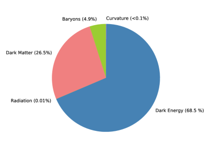
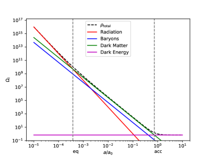
Figure 1.1: Left Panel: The composition of the universe today. Right Panel: The dynamics of the energy density contribution of the different constituents of the universe. The left dashed vertical line denotes the time at matter-radiation equality $(\mathrm{eq})$ when the first atoms form while the right dashed vertical one denotes the time when the dark energy dominated the universe energy budget driving an accelerated expansion $(\mathrm{acc})$.

1.4 The Problems of the Hot Big Bang Universe

After having presented the fundamental notions and the theoretical framework of a homogeneous and an isotropic universe and giving a brief thermal history of our universe dictated by the Hot Big Bang theory we feature here the basic shortcomings of the standard Hot Big Bang cosmology that motivated inflation  [47, 48, 49, 50, 51]. Actually, we will refer to two of them: the horizon problem and the flatness problem.

1.4.1 The horizon problem

The horizon problem  [77, 78] or large scale homogeneity problem is qualitatively the fact that regions separated by distances greater than the speed of light times the age of the universe (no causal connected regions) are observed to have similar density and temperature fluctuations up to $10^{-5}$, a fact which is contradicting since they should not know each other due to the principle of special relativity for the finitude of the speed of light. Therefore, there should have been an information exchange between these regions in the past. More quantitatively, we can see the evolution of the horizon and of physical lengths during radiation and matter dominating epochs. In particular, from equation Eq. (1.22) one obtains for radiation domination (RD) ($w=1/3$) and matter domination (MD) ($w=0$) that

$$R_{H}=\begin{cases}\frac{4}{3}M_{\scriptscriptstyle{\mathrm{Pl}}}\mathchoice{{\hbox{$\displaystyle\sqrt{\frac{3}{\rho_{\mathrm{ini}}}\,}$}\lower 0.4pt\hbox{\vrule height=9.56943pt,depth=-7.65558pt}}}{{\hbox{$\textstyle\sqrt{\frac{3}{\rho_{\mathrm{ini}}}\,}$}\lower 0.4pt\hbox{\vrule height=6.6986pt,depth=-5.3589pt}}}{{\hbox{$\scriptstyle\sqrt{\frac{3}{\rho_{\mathrm{ini}}}\,}$}\lower 0.4pt\hbox{\vrule height=4.96646pt,depth=-3.97319pt}}}{{\hbox{$\scriptscriptstyle\sqrt{\frac{3}{\rho_{\mathrm{ini}}}\,}$}\lower 0.4pt\hbox{\vrule height=4.96646pt,depth=-3.97319pt}}}\left(1+\frac{3}{2}\mathchoice{{\hbox{$\displaystyle\sqrt{\frac{\rho_{\mathrm{ini}}}{3}\,}$}\lower 0.4pt\hbox{\vrule height=9.4722pt,depth=-7.57779pt}}}{{\hbox{$\textstyle\sqrt{\frac{\rho_{\mathrm{ini}}}{3}\,}$}\lower 0.4pt\hbox{\vrule height=6.63054pt,depth=-5.30446pt}}}{{\hbox{$\scriptstyle\sqrt{\frac{\rho_{\mathrm{ini}}}{3}\,}$}\lower 0.4pt\hbox{\vrule height=5.0996pt,depth=-4.0797pt}}}{{\hbox{$\scriptscriptstyle\sqrt{\frac{\rho_{\mathrm{ini}}}{3}\,}$}\lower 0.4pt\hbox{\vrule height=5.0996pt,depth=-4.0797pt}}}\frac{t-t_{\mathrm{ini}}}{M_{\scriptscriptstyle{\mathrm{Pl}}}}\right),\mathrm{\;for\;RD}\\ M_{\scriptscriptstyle{\mathrm{Pl}}}\mathchoice{{\hbox{$\displaystyle\sqrt{\frac{3}{\rho_{\mathrm{ini}}}\,}$}\lower 0.4pt\hbox{\vrule height=9.56943pt,depth=-7.65558pt}}}{{\hbox{$\textstyle\sqrt{\frac{3}{\rho_{\mathrm{ini}}}\,}$}\lower 0.4pt\hbox{\vrule height=6.6986pt,depth=-5.3589pt}}}{{\hbox{$\scriptstyle\sqrt{\frac{3}{\rho_{\mathrm{ini}}}\,}$}\lower 0.4pt\hbox{\vrule height=4.96646pt,depth=-3.97319pt}}}{{\hbox{$\scriptscriptstyle\sqrt{\frac{3}{\rho_{\mathrm{ini}}}\,}$}\lower 0.4pt\hbox{\vrule height=4.96646pt,depth=-3.97319pt}}}\left(1+\frac{3}{2}\mathchoice{{\hbox{$\displaystyle\sqrt{\frac{\rho_{\mathrm{ini}}}{3}\,}$}\lower 0.4pt\hbox{\vrule height=9.4722pt,depth=-7.57779pt}}}{{\hbox{$\textstyle\sqrt{\frac{\rho_{\mathrm{ini}}}{3}\,}$}\lower 0.4pt\hbox{\vrule height=6.63054pt,depth=-5.30446pt}}}{{\hbox{$\scriptstyle\sqrt{\frac{\rho_{\mathrm{ini}}}{3}\,}$}\lower 0.4pt\hbox{\vrule height=5.0996pt,depth=-4.0797pt}}}{{\hbox{$\scriptscriptstyle\sqrt{\frac{\rho_{\mathrm{ini}}}{3}\,}$}\lower 0.4pt\hbox{\vrule height=5.0996pt,depth=-4.0797pt}}}\frac{t-t_{\mathrm{ini}}}{M_{\scriptscriptstyle{\mathrm{Pl}}}}\right),\mathrm{\;for\;MD}\end{cases}$$ (1.32)

On the other hand, the physical distances evolve as we showed before as

$$R_{\mathrm{phys}}=a(t)r=\begin{cases}a_{\mathrm{ini}}\left(1+\frac{3}{2}\mathchoice{{\hbox{$\displaystyle\sqrt{\frac{\rho_{\mathrm{ini}}}{3}\,}$}\lower 0.4pt\hbox{\vrule height=9.4722pt,depth=-7.57779pt}}}{{\hbox{$\textstyle\sqrt{\frac{\rho_{\mathrm{ini}}}{3}\,}$}\lower 0.4pt\hbox{\vrule height=6.63054pt,depth=-5.30446pt}}}{{\hbox{$\scriptstyle\sqrt{\frac{\rho_{\mathrm{ini}}}{3}\,}$}\lower 0.4pt\hbox{\vrule height=5.0996pt,depth=-4.0797pt}}}{{\hbox{$\scriptscriptstyle\sqrt{\frac{\rho_{\mathrm{ini}}}{3}\,}$}\lower 0.4pt\hbox{\vrule height=5.0996pt,depth=-4.0797pt}}}\frac{t-t_{\mathrm{ini}}}{M_{\scriptscriptstyle{\mathrm{Pl}}}}\right)^{1/2},\mathrm{\;for\;RD}\\ a_{\mathrm{ini}}\left(1+\frac{3}{2}\mathchoice{{\hbox{$\displaystyle\sqrt{\frac{\rho_{\mathrm{ini}}}{3}\,}$}\lower 0.4pt\hbox{\vrule height=9.4722pt,depth=-7.57779pt}}}{{\hbox{$\textstyle\sqrt{\frac{\rho_{\mathrm{ini}}}{3}\,}$}\lower 0.4pt\hbox{\vrule height=6.63054pt,depth=-5.30446pt}}}{{\hbox{$\scriptstyle\sqrt{\frac{\rho_{\mathrm{ini}}}{3}\,}$}\lower 0.4pt\hbox{\vrule height=5.0996pt,depth=-4.0797pt}}}{{\hbox{$\scriptscriptstyle\sqrt{\frac{\rho_{\mathrm{ini}}}{3}\,}$}\lower 0.4pt\hbox{\vrule height=5.0996pt,depth=-4.0797pt}}}\frac{t-t_{\mathrm{ini}}}{M_{\scriptscriptstyle{\mathrm{Pl}}}}\right)^{2/3},\mathrm{\;for\;MD}\end{cases}$$

Thus, one can infer that the horizon scale, $R_{\mathrm{H}}$ grows faster than physical distances both in the RD and MD eras. Consequently, in the past there should have been regions which were causally disconnected. However, our universe is extremely homogeneous and isotropic (e.g. CMB temperature fluctuations $\frac{\delta T}{T}\sim 10^{-5}$ on angular scales larger than $1\deg$, which corresponds to the horizon scale at the time of the emission of CMB).

1.4.2 The Flatness Problem

Regarding the flatness problem one can see how the $\Omega$ parameter, related to the spatial curvature of the universe through Eq. (1.19), evolves in time. From Eq. (1.19) we see that if the universe is perfectly flat today then $\Omega=1$ at all times. If however there is a small curvature $K\neq 0$ then $\Omega$ will depend on time. Below, we consider the case where $K=+1\neq 0$ for the RD and MD eras. Knowing then that $\rho_{r}\propto a^{-4}$ for the RD era and $\rho_{m}\propto a^{-3}$ for the MD era and taking into account that $H^{2}\propto\rho_{\mathrm{t}}$, Eq. (1.19) is equivalent to

$$\Omega-1\propto\begin{cases}a^{2},\mathrm{\;for\;RD}\\ a,\mathrm{\;for\;MD}\end{cases}$$ (1.33)

Consequently, knowing that $\Omega\sim 0.01$ today and that $T_{\mathrm{r}}\sim 1/a$ one can easily infer that at the beginning of the radiation dominated era, which here we identify with the epoch of BBN where $T_{\mathrm{BBN}}\sim 1\mathrm{MeV}$,

$$\frac{|\Omega-1|_{T=T_{\mathrm{BBN}}}}{|\Omega-1|_{T=T_{0}}}\approx\left(\frac{a^{2}_{\mathrm{BBN}}}{a^{2}_{0}}\right)\approx\left(\frac{T^{2}_{0}}{T^{2}_{\mathrm{BBN}}}\right)\approx O(10^{-16})$$ (1.34)

where $T_{0}\sim 10^{-13}eV\sim 2.7K$ is the present temperature of CMB. Therefore, in order to recover the value $\Omega_{0}-1\sim 1$ today we must assume that the value of $\Omega-1$ at early times (Planck era) is perfectly fine-tuned to a value very close to zero $10^{-16}$ but not exactly zero! That is the flatness problem, also dubbed as the “fine-tuning” problem and lies in understanding the mysterious mechanism which led the universe to start its expansion with almost spatially flat initial conditions  [79, 80].

1.4.2.1 The flatness problem and the entropy conservation

Let us see here, how the flatness problem is related to the assumption of the adiabatic expansion. Equation (1.19) can be recast in the RD era, where $\rho_{r}=\frac{\pi^{2}}{30}g_{*}(T)T^{4}$ with $g_{*}$ being the number of relativistic degrees of freedom when the universe’s temperature is $T$, as follows

$$\Omega-1=\frac{90}{\pi^{2}g_{*}(T)}\frac{kM_{\scriptscriptstyle{\mathrm{Pl}}}^{2}}{a^{2}T^{4}}=\left[\frac{1440}{\pi^{2}g_{*}(T)}\right]^{1/3}\frac{kM^{2}_{Pl}}{S^{\frac{2}{3}}T^{2}},$$ (1.35)

where in the last equality we use the fact the entropy $S$ is defined as $S\equiv sV$, where the entropy density $s$ reads as $s=\frac{2\pi^{2}}{45}g_{*}(T)T^{3}$ and the volume $V=a^{3}$. Thus, Eq. (1.35) at the BBN time reads as

$$|\Omega-1|_{T=T_{\mathrm{BBN}}}=\left[\frac{1440}{\pi^{2}g_{*}(T)}\right]^{1/3}\frac{M_{\scriptscriptstyle{\mathrm{Pl}}}^{2}}{S^{2/3}_{\mathrm{BBN}}T^{2}_{\mathrm{BBN}}}\approx 10^{-16}$$ (1.36)

In the last step, we used the fact that the entropy in a comoving volume is conserved and it is equal to $10^{90}$ according to observational evidence from the matter-antimatter asymmetry [81] and that the number of relativistic degrees of freedom at BBN time, where $T_{\mathrm{BBN}}\sim 1\mathrm{MeV}$, is $\mathrm{g}_{*}(T_{\mathrm{BBN}})=106.75$, having accounted only for the SM particles. Evidently, we find again the same “fine-tuning” problem as before in which the universe should have started with almost spatially flat initial conditions. However, now this “fine-tuning” problem arises because we have adopted the assumption of entropy conservation.

1.4.3 Solving the problems

Regarding the horizon problem mentioned above, in order to solve it, the universe has to pass through a primordial period in which physical lengths $R_{\mathrm{phys}}$ grow faster than the horizon scale $H^{-1}$. Specifically, if there is a period in which physical lengths grow faster than the horizon then the photons that appear to be causally disconnected in the time of last scattering (when CMB was emitted) where $\lambda>H^{-1}$ had the chance to “talk” to each other in a primordial cosmic era where $\lambda<H^{-1}$. In this way, we recover the homogeneity and isotropy of CMB solving the horizon problem. This last condition can be expressed in terms of the evolution of the scale factor $a(t)$. Thus, since $\lambda\propto a$ and $H^{-1}=a/\dot{a}$ we should impose a period in the cosmic history where

$$\left(\frac{\lambda}{H^{-1}}\right)^{.}=\ddot{a}>0.$$ (1.37)

This equation can be recast, using Eq. (1.17) and the fact that during this early cosmic era the universe’s energy content is dominated by a fluid $X$ with an equation-of-state parameter $w_{\mathrm{X}}=p/\rho$, in the following form

$$w_{\mathrm{X}}<-1/3.$$ (1.38)

In order to solve now the flatness/entropy problem, we should demand that in an initial era of the cosmic history before the onset of the radiation era, the parameter $\Omega-1$ should decrease allowing in this way to obtain very low values of the order of $10^{-16}$. To ensure this, one can assume that the universe during this early era is prevailed by a fluid $X$ with equation of state $w_{\mathrm{X}}$. Combining therefore Eq. (1.19), Eq. (1.21) and Eq. (1.23) one straightforwardly obtains that

$$\Omega-1\propto a^{1+3w_{\mathrm{X}}}$$ (1.39)

Consequently, in order for $\Omega-1$ to decrease one requires that

$$w_{\mathrm{X}}<-1/3.$$ (1.40)

This last condition, $w_{\mathrm{X}}<-1/3$ for the solution of the flatness/entropy problem is the same as the condition to address the horizon problem and defines the inflationary period in the cosmic expansion. During this period, the universe expands in an accelerated way, i.e. $\ddot{a}>0$ and the $\Omega$ parameter at the end of inflation is forced to take a value very close to one, but not exactly one, independently of its initial value.

At this point, we should stress out that during inflation the universe expands in an adiabatic way, i.e. there is no entropy production. More rigorously, this means that one should ensure the covariant conservation of the stress energy tensor, i.e. $\nabla_{\mathrm{\mu}}T^{\mathrm{\mu\nu}}=0$. To ensure however the transition to the radiation era the universe should pass through a non adiabatic period of reheating during which an enormous amount of entropy is generated through relativistic degrees of freedom, solving in this way naturally the flatness/entropy problem. This early phase transition era is broadly quoted as (pre)reheating and was one of the topics studied within my PhD where we studied together with by collaborators the production of PBHs during the period of preheating in the context of single-field inflationary models.

Chapter 2 PBH Formation

In this chapter, we introduce the fundamentals of PBH physics. Firstly, we give the basic theoretical framework in the field of PBH research by introducing the notions of the PBH mass function, the PBH characteristic scale and the PBH threshold. Then, we present briefly the current observational status in the domain of PBH physics by describing the different observational constraints on the abundance of PBHs as a function of their mass. Finally, we underlie the implications of PBHs in cosmology.

2.1 PBH Basics

2.1.1 The PBH Mass

As we saw in the discussion after Eq. (1.26) the expression which relates the mass inside the Hubble radius and the Hubble radius is the same expression used for the definition of the black hole apparent horizon in spherical symmetry. This fact, as mentioned in Sec. 1.1.6, reflects the common physical nature of the cosmological horizon and the black hole apparent horizon from the point of view of general relativity. In particular, the black hole apparent horizon is the asymptotic location of the outermost trapped surface for outgoing light-rays whereas the cosmological horizon is the innermost trapped surface for incoming light rays. One then expects that the mass of a PBH is the same with the mass inside the horizon at PBH formation epoch, which is considered roughly as the time at which the PBH characteristic scale crosses the Hubble radius. However, more accurate analysis shows that the mass of a PBH is a fraction of the mass inside the horizon at the time of PBH formation and reads as

$$m_{\mathrm{PBH}}=\gamma M_{\mathrm{H}},$$ (2.1)

where $\gamma\sim O(1)$ is an efficiency parameter encapsulating the details of the gravitational collapse.

At this point, one should stress out the importance of scaling laws in PBH formation process firstly noted by Jedmazik and Niemeyer  [82] and further investigated by Musco et al.  [83, 84] which can refine the computation of the PBH mass. Specifically, when the local/mean energy density excess is sufficiently close to the critical threshold $\delta_{\mathrm{c}}$, i.e. $|\delta-\delta_{\mathrm{c}}|\ll 1$, then the refined PBH mass is given by the following scaling law,

$$m_{\mathrm{PBH}}\propto M_{\mathrm{H}}\left(\delta-\delta_{\mathrm{c}}\right)^{p},$$ (2.2)

where $p\simeq 0.37$ is a universal exponent. The above critical scaling behavior was already found in the context of spherical symmetric collapse of a massless scalar field firstly studied by Choptuik  [85] and further explored by subsequent studies  [86, 87]. Here, it is important to mention that the scaling law in Eq. (2.2) breaks down when one approaches very small values of the difference $\delta-\delta_{\mathrm{c}}$ due to generation of shock waves in nearly critical collapse, imposing in this way a minimum mass for $m_{\mathrm{PBH}}$ at the order of $10^{-4}$ of the mass inside the horizon  [88].

2.1.2 The PBH characteristic scale

Having defined before the PBH mass as the horizon mass at the time of PBH formation, approximately equal to the time at which the PBH characteristic scale crosses the Hubble radius, one will inevitably ask the question what is this characteristic scale. In general, assuming spherical symmetry, it is considered to be roughly equal to the scale at which the local energy density excess of the overdensity/energy density profile, $\delta(r)$, at PBH formation time is zero. However, there are energy density profiles which are always positive, such as the Gaussian one, which give an infinite PBH scale. These profiles are called non-compensated profiles whereas profiles in which $\delta(r)$ becomes negative at some point are the compensated ones. See Fig. 2.1 in which a compensated and a non-compensated energy density profiles are shown together with the respective PBH scales.

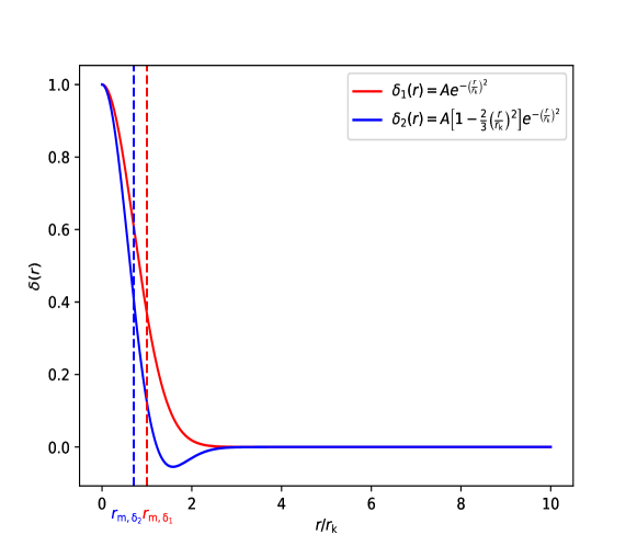
Figure 2.1: The PBH scale for a compensated and a non-compensated energy density profile $\delta(r)$. The blue solid line represents a Gaussian (non-compensated) energy density profile, denoted as $\delta_{1}(r)$, whereas the red solid line stands for a Mexican-hat (compensated) profile, denoted as $\delta_{2}(r)$. In both profiles, the parameters $A$ and $r_{\mathrm{k}}$ are chosen to be $A=r_{\mathrm{k}}=1$. By making use of Eq. (2.4), we plot with the vertical dashed blue line the PBH scale in the case of the Mexican-hat profile and with the vertical dashed red line the PBH scale for the Gaussian profile.

For this reason, the PBH characteristic scale is usually defined in a more refined way for any type of energy density profiles by using the notion of the compaction function, firstly introduced by Shibata $\&$ Sasaki in  [90] and then recently used by Musco  [89]. The compaction function $\mathcal{C}$ is defined in a similar fashion as the Schwarzschild condition for the formation of a black hole apparent horizon, $R=2GM$ and can be seen as a local measure of the gravitational potential. In particular, it is defined as twice the local mass-excess over the areal radius and reads as

$$\mathcal{C}(r,t)\equiv 2\frac{\delta M(r,t)}{R(r,t)},$$ (2.3)

where $\delta M(r,t)$ is the mass excess of a local overdense region and $R(r,t)=a(t)r$ is the areal radius of this region. Then, the characteristic comoving scale, $r_{\mathrm{m}}$ of the overdense region, is defined as the the position of the maximum of the compaction function, usually computed on the superhorizon regime, where the compaction function becomes time-independent  [89].

$$\mathcal{C}^{\prime}(r_{\mathrm{m}})=0.$$ (2.4)

In Fig. 2.1, one clearly sees that if using the condition 2.4, they can clearly determine a finite PBH scale even for non-compensated energy density profiles, like the Gaussian one.

2.1.3 The PBH Mass Function

We consider here the standard PBH formation scenario during which PBHs form out of primordial energy density fluctuations when the local/mean energy density excess of an overdense region is larger than a critical threshold, $\delta_{\mathrm{c}}$. In this case, when $\delta>\delta_{\mathrm{c}}$ the overdense region stops expanding and collapses against the pressure of the background medium, forming in this way a PBH. Consequently, in the context of Press-Schechter formalism  [91], the PBH mass function is defined as the probability that the local/mean energy density excess of an overdense region of mass $M$ is larger than a critical threshold $\delta_{\mathrm{c}}$:

$$\beta(M)\equiv P\left[\delta>\delta_{\mathrm{c}}\right]=\int_{\delta_{\mathrm{c}}}^{\infty}P(M,\delta)\mathrm{d}\delta,$$ (2.5)

where $P(M,\delta)$ is the probability density function (PDF) of the density fluctuations which can potentially collapse and form PBHs. The PBH mass function is a very important quantity since it is the one constrained by observational probes. See  [29] for a review about the constraints on $\beta(M)$.

Regarding the limitations of the Press-Schechter formalism, which render approximate this approach in some regimes one should mention the well known cloud-in-cloud problem  [92] in which small overdense regions which are parts of larger overdensities and collapse to form PBHs are not taken into account leading in this way to an underestimation of the PBH abundance. In addition, the Press-Schechter approach assumes an underlying Gaussian density field which is not only the case. To address thus these problems, the excursion-set formalism was introduced initially by  [93] and further developed by  [94, 95] to tackle mainly the cloud-in-cloud problem, in which one should treat the density fluctuation, $\delta$, as a random variable and solve stochastic model equations to obtain analytically  [96, 97, 98] or numerically  [95, 99] the mass function. Regarding now the limitations on the Gaussian nature of the underlying density fields, there have been proposed some extensions of the Press-Schechter formalism in the context of non-Gaussian regimes  [100, 101] as well as studies of non-Gaussian initial conditions in the context of the excursion set theory regarding the halo mass functions  [102, 103].

At this point, one should stress out that the PBH mass function is also often calculated in the context of peak theory  [104] which studies the statistics of the peaks of a Gaussian density field and which assumes that a PBH is formed when a local density peak exceeds a certain threshold value. The peak theory approach similarly to the Press-Schechter formalism suffers as well from the Gaussian assumption for the underlying density field.

Here, one should point out that the Press-Press-Schechter forrmalism, the peak theory as well as the excursion set theory are not related to the companction function method introduced before to compute the PBH characteristic scale.

2.1.4 The PBH Threshold

As we saw before, in order to determine the PBH mass function one should have an expression for the PDF of the density fluctuations which can collapse and form PBHs as well as an expression of the critical threshold value, $\delta_{\mathrm{c}}$. The PDF of the density fluctuations is rather model dependent and one cannot say much more about it without specifying the specific model which can give rise to PBH formation. The critical threshold however, in most cases, depends on the characteristic scale and the shape of the collapsing overdensity region, the time at which the gravitational collapse is taking place  [10] as well as on the details of the surroundings. In what follows, we will try to give a brief summary in a historical order of the analytic and numerical works done so far for the determination of the critical PBH formation threshold $\delta_{\mathrm{c}}$.

2.1.4.1 Early Approaches

The first historical attempt for the determination of the PBH formation threshold was done by Bernard Carr and Stephen Hawking between 1974 and 1975  [9, 10] where they used a simplified Jeans instability criterion in the context of Newtonian gravity to determine $\delta_{\mathrm{c}}$. Specifically, they required that an overdense region in the early Universe can collapse to form a PBH if its characteristic scale is larger than the Jeans length at maximum expansion. This led B. Carr to his famous result that $\delta_{\mathrm{c}}\sim w$ at horizon crossing time, where $w$ is the equation-of-state parameter defined in Sec. 1.1.5. Afterwards, the PBH formation threshold was studied for the first time numerically through hydrodynamic simulations by some pioneering works from Nadezhin, Novikov $\&$ Polnarev in 1978  [105], Bicknell $\&$ Henriksen in 1979  [106] and Novikov $\&$ Polnarev in 1980  [107].

Then, after a break of almost 20 years, the PBH formation threshold was studied again by highly sophisticated simulations this time performed in 1999 by Niemeyer $\&$ Jedmazik  [82] and Shibata $\&$ Sasaki  [90] which expressed the PBH formation threshold in terms of the energy density and curvature perturbation and which gave the same range for $\delta_{\mathrm{c}}$ varying between $0.3$ and $0.5$ depending on the shape of the energy density/curvature profiles considered.

2.1.4.2 Contemporary Approaches

In the last decades, a lot of progress has been made in the research for the determination of the PBH formation threshold both at the analytic as well as at the numerical level.

In particular, T.Harada, C-M. Yoo $\&$ K. Kohri in 2013  [108] considered a “three zone” spherical symmetric model for the description of the energy density field in which an initially sharply peaked overdense region is modeled as a homogeneous core (closed universe) surrounded by an underdense shell which separates the overdense region from the expanding background universe. In the end, after comparing the time at which the pressure sound wave crosses the overdensity with the onset time of the gravitational collapse they updated the PBH formation threshold value obtained by Carr in 1975 and in the uniform Hubble gauge their expression for $\delta_{\mathrm{c}}$ as a function of the equation-of-state parameter $w$ reads as:

$$\delta_{\mathrm{c}}=\sin^{2}\left(\frac{\pi\mathchoice{{\hbox{$\displaystyle\sqrt{w\,}$}\lower 0.4pt\hbox{\vrule height=4.30554pt,depth=-3.44446pt}}}{{\hbox{$\textstyle\sqrt{w\,}$}\lower 0.4pt\hbox{\vrule height=4.30554pt,depth=-3.44446pt}}}{{\hbox{$\scriptstyle\sqrt{w\,}$}\lower 0.4pt\hbox{\vrule height=3.01389pt,depth=-2.41113pt}}}{{\hbox{$\scriptscriptstyle\sqrt{w\,}$}\lower 0.4pt\hbox{\vrule height=2.15277pt,depth=-1.72223pt}}}}{1+3w}\right).$$ (2.6)

At this point, it is important to stress out that the above mentioned expression for $\delta_{\mathrm{c}}$ is valid for at least the cases where $w\ll 1$ where one expects negligible pressure gradients which can not break up the homogeneity of the overdense region.

Some years later, knowing the dependence of $\delta_{\mathrm{c}}$ on the shape of the initial energy density perturbation which collapses to a PBH already since the early numerical works in 1999 from Niemeyer $\&$ Jedmazik  [82] and Shibata $\&$ Sasaki  [90], the authors of [109] quantified this effect by introducing a shape parameter in terms of the compaction function defined in Eq. (2.3) through which one can describe the shape of the initial density perturbation around the peak of the collapsing overdensity. With “shape” here, one refers to the broadness or sharpness of the energy density perturbation around its peak. In particular, the shape parameter is related to the second derivative of the compaction function at the comoving characteristic scale of the perturbation and it is defined on superhorizon scales where the compaction function is time independent as

$$\alpha\equiv-\frac{r^{2}_{\mathrm{m}}\mathcal{C}^{\prime\prime}(r_{\mathrm{m}})}{4\mathcal{C}(r_{\mathrm{m}})}$$ (2.7)

Here, it is important to mention that the compaction function computed at $r_{\mathrm{m}}$ is equal, as it can be straightforwardly checked, to the average energy density excess over a volume of radius $r_{\mathrm{m}}$,

$$\delta_{\mathrm{m}}\equiv\frac{1}{V}\int^{r_{\mathrm{m}}}_{0}4\pi r^{2}\delta(r)=\mathcal{C}(r_{\mathrm{m}}),$$ (2.8)

where $V=4\pi r^{3}_{\mathrm{m}}/3$ and $\delta(r)$ is the superhorizon time independent energy density perturbation. Consequently, one can formulate the PBH formation criterion by requiring that a PBH forms when the compaction function at $r_{\mathrm{m}}$, $\mathcal{C}(r_{\mathrm{m}})$ or equivalently the average perturbation amplitude, $\delta_{\mathrm{m}}$ is greater than a critical threshold which depends on the shape of the initial energy density profile as well as on the characteristic scale, $r_{\mathrm{m}}$ of the collapsing overdense region. This threshold was studied numerically in  [110] and recently in  [89].

Furthermore, it is important to point out here that the authors of  [109], by making use of an effective basis for the initial curvature profile which can reproduce any realistic curvature for the calculation of the PBH formation threshold, deduced in the case of PBH formation during a radiation era a universal analytic threshold for the average compaction function as a function of the shape parameter defined in Eq. (2.7). Their analytic expression for the threshold reads as

$$\delta_{\mathrm{c}}=\frac{4}{15}e^{-\frac{1}{\alpha}}\frac{\alpha^{1-\frac{5}{2\alpha}}}{\Gamma\left(\frac{5}{2\alpha}\right)-\Gamma\left(\frac{5}{2\alpha},\frac{1}{\alpha}\right)},$$ (2.9)

where $\Gamma(x)$ is the gamma function and $\Gamma(x,y)$ is the incomplete gamma function and $\alpha$ is the shape parameter given by Eq. (2.7). The work of  [109] was generalized for an arbitrary equation-of-state parameter $w$ and it was found that for $w>1/3$ one can find an analytic formula for $\delta_{\mathrm{c}}$ as a function of $\alpha$ and $w$. We do not give here the full expression since it is quite complicated. For $w<1/3$ the determination of an analytic PBH formation threshold remains an open issue given that in this regime the full shape of the compaction function is necessary.

At this point it is very important to underlie the huge interest raised recently in the role of non-linearities  [111, 112, 113, 114] and non-Gaussianities  [115, 116, 117, 118, 119] for the determination of the PBH formation threshold as well as the dependence of the PBH abundance  [120] on the details of the initial power spectrum of curvature perturbations which gave rise to PBHs  [121, 122, 123]. In addition, we should mention that the majority of the research work conducted in the literature assumes spherical collapse of the initial perturbations which leads to the production of non rotating PBHs. However, in a more realistic case, one can in principle expect non spherical collapse of the initial overdense regions which in general induces velocity field generation and therefore rotation effects. This last aspect was studied both analytically  [124] and numerically  [125] showing that in principle a non-spherical collapse can make harder the PBH formation leading to the increase of the PBH formation threshold. Finally, regarding rotation, which has not necessarily generated due to non-spherical gravitational collapse, there has been been done a lot of analytic  [126, 127] and numerical work  [128, 129] pointing out that the PBH formation threshold in general increases with the angular momentum which in its turn prevents the gravitational collapse.

2.1.5 The PBH formation threshold in a time-dependent $w$ background

Having reviewed early and contemporary approaches about the determination of the PBH formation threshold, we extract here for the first time, to the best of our knowledge, the PBH formation threshold, $\delta_{\mathrm{c}}$, in the case of a time-dependent equation-of-state parameter, $w$. To do that, we follow closely and generalize the analytic treatment of  [108], in which one can compute $\delta_{\mathrm{c}}$ in the uniform Hubble gauge defined in the next subsections, by considering the “three-zone” model adopted in  [108]. In particular, in this subsection, we initially introduce the “three-zone” model, then we compute the energy density perturbation of the overdensity region in the uniform Hubble gauge and finally we present a scheme to compute the PBH formation threshold in the case of a time-dependent equation-of-state parameter.

2.1.5.1 The “three-zone” model

In the spherically symmetric “three-zone” model, the overdense region is a homogeneous core (closed universe) surrounded by a thin underdense spherical shell which compensates the overdensity and separates the overdense region from the expanding background universe. See below Fig. 2.2.

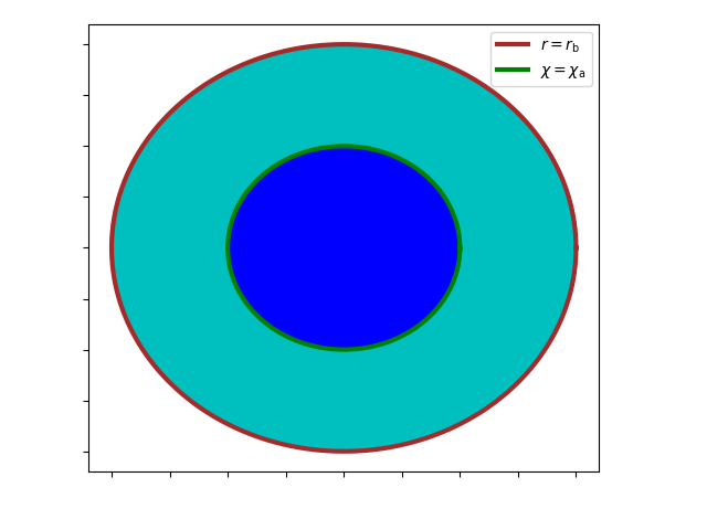
Figure 2.2: The spherical “three-zone” model: The overdensity region is shown in blue and it is surrounded by a spherical underdense layer depicted with cyan. The boundary between the overdensity region and the spherical underdense layer is shown with the green circumference at $\chi=\chi_{\mathrm{a}}$ whereas the boundary between the underdense layer and the FLRW flat background is depicted with the brown circumference at $r=r_{\mathrm{b}}$.

On the one hand, the background metric corresponds to a flat FLRW universe and reads as

$$\mathrm{d}s^{2}=-\mathrm{d}t^{2}+a^{2}_{\mathrm{b}}(t)\left(\mathrm{d}r^{2}+r^{2}\mathrm{d}\Omega^{2}\right),$$ (2.10)

where $\mathrm{d}\Omega^{2}$ is the line element of a unit two-sphere and $a_{\mathrm{b}}(t)$ is the scale factor of the background universe. The respective Friedmann equation reads as

$$H^{2}_{\mathrm{b}}=\left(\frac{\dot{a}_{\mathrm{b}}}{a_{\mathrm{b}}}\right)^{2}=\frac{\rho_{\mathrm{b}}}{3M_{\scriptscriptstyle{\mathrm{Pl}}}^{2}},$$ (2.11)

where $\rho_{\mathrm{b}}$ and $H_{\mathrm{b}}$ is the energy density and the Hubble parameter of the background universe.

On the other hand, the overdense region corresponds to a close ($K=1$) FLRW universe with a metric

$$\mathrm{d}s^{2}=-\mathrm{d}t^{2}+a^{2}(t)\left(\mathrm{d}\chi^{2}+\sin^{2}\chi\mathrm{d}\Omega^{2}\right)$$ (2.12)

and a Friedmann equation

$$\left(\frac{\dot{a}}{a}\right)^{2}=\frac{\rho}{3M_{\scriptscriptstyle{\mathrm{Pl}}}^{2}}-\frac{1}{a^{2}},$$ (2.13)

where $\rho$ is the energy density of the overdense region.

The underdense spherical shell is matched to the closed FLRW universe describing the overdensity at $\chi=\chi_{\mathrm{a}}$ while the flat FLRW background universe is matched to the the compensating underdense layer at $r=r_{\mathrm{b}}$. Therefore, the areal radius at the edge of the overdense region, $R_{\mathrm{a}}$ as well as that a the edge of the surrounding underdense spherical shell read as

$$R_{\mathrm{a}}=a\sin\chi_{\mathrm{a}},\quad R_{\mathrm{b}}=a_{\mathrm{b}}r_{\mathrm{b}}$$ (2.14)

2.1.5.2 Defining the energy density perturbation on the uniform Hubble gauge

Then, having introduced the spherical “three-zone” model, we extract here the energy density perturbation at horizon crossing time on the uniform Hubble gauge, in which the Hubble parameters of the overdensity and that of the background are the same, i.e. $H=H_{\mathrm{b}}$. To do so, we firstly introduce the energy density parameter, $\Omega$ of the overdense region defined as

$$\Omega\equiv\frac{\rho}{3M_{\scriptscriptstyle{\mathrm{Pl}}}^{2}H^{2}}=1+\frac{1}{a^{2}H^{2}},$$ (2.15)

where in the last equality we have used Eq. (2.13). Then, using the expression for the areal radius at $\chi=\chi_{\mathrm{a}}$, i.e. $R_{\mathrm{a}}=a\sin\chi_{\mathrm{a}}$, as well as the definition of the horizon scale, i.e. $R_{\mathrm{H}}=H^{-1}$, one can find straightforwardly that

$$(\Omega-1)\left(\frac{R_{\mathrm{a}}}{R_{\mathrm{H}}}\right)^{2}=\sin^{2}\chi_{\mathrm{a}},$$ (2.16)

an expression which relates $\Omega$ with the scale of the overdensity. In addition, one can relate $\Omega$ with the energy density perturbation of the overdense region with respect to the background defined as

$$\delta\equiv\frac{\rho-\rho_{\mathrm{b}}}{\rho_{\mathrm{b}}}.$$ (2.17)

Specifically, by solving Eq. (2.17) for $\rho$ and substituting $\rho$ in Eq. (2.15) one can obtain that

$$\Omega=(1+\delta)\left(\frac{H_{\mathrm{b}}}{H}\right)^{2},$$ (2.18)

where $\rho_{\mathrm{b}}$ has been expressed in terms of $H_{\mathrm{b}}$ through Eq. (2.11). Then, one can extract the energy density perturbation at horizon crossing time, $\delta_{\mathrm{H}}$, at the time when $R_{\mathrm{a}}=H^{-1}_{\mathrm{b}}$, by solving for $\delta$ Eq. (2.18) and substituting $\Omega$ from Eq. (2.16). Finally, one gets that

$$\delta_{\mathrm{H}}=\left(\frac{H}{H_{\mathrm{b}}}\right)^{2}-\cos^{2}\chi_{\mathrm{a}}.$$ (2.19)

In the uniform Hubble time slicing, in which $H=H_{\mathrm{b}}$, Eq. (2.19) becomes

$$\delta^{\mathrm{UH}}_{\mathrm{H}}=\sin^{2}\chi_{\mathrm{a}},$$ (2.20)

where $\delta^{\mathrm{UH}}_{\mathrm{H}}$ denotes $\delta$ in the uniform Hubble gauge at horizon crossing time. We should note here that the above expression for $\delta^{\mathrm{UH}}_{\mathrm{H}}$ does not depend on the equation of state of the universe at PBH formation time.

2.1.5.3 The PBH formation threshold refined

After expressing the energy density perturbation in the uniform Hubble gauge we compute now the PBH formation threshold in the case of a time dependent equation-of-state parameter. In particular, we compute the threshold by comparing the pressure and the gravitational force or equivalently the sound crossing time over the radius of the overdensity and the free fall time from the maximum expansion to complete collapse. To do so, we redefine the scale factor $a$ and the cosmic time $t$ such as that the Friedmann equation for the overdensity, Eq. (2.13) takes the Tolman-Bondi form, valid for the dust case, which has an analytic parametric solution. Specifically, we redefine $a$ and $t$ as follows

$$\tilde{a}=ae^{3I(a)}$$ (2.21)

$$\mathrm{d}\tilde{t}=\mathrm{d}te^{3I(a)}\left[1+3w(a)\right]$$ (2.22)

where $I\left(a\right)\equiv\int_{a_{\mathrm{ini}}}^{a}\frac{w(x)}{x}\mathrm{d}x$ and the index $\mathrm{ini}$ denotes the initial time. Then, solving the continuity equation (1.18) for a time-dependent equation-of-state parameter and using the coordinate transformation of Eq. (2.21), the Friedmann equation of the overdensity region (2.13) can be written in a dust form as

$$\left(\frac{\mathrm{d}\tilde{a}}{\mathrm{d}\tilde{t}}\right)^{2}=\frac{A}{\tilde{a}}-1,$$ (2.23)

where $A=\frac{\rho_{\mathrm{ini}}a^{3}_{\mathrm{ini}}}{3M_{\scriptscriptstyle{\mathrm{Pl}}}^{2}}$ and we have used the fact that $\frac{\mathrm{d}\tilde{a}}{\mathrm{d}\tilde{t}}=\frac{\mathrm{d}a}{\mathrm{d}t}$. The above equation can be integrated and gives a parametric solution of the form

$$\tilde{a}=\tilde{a}_{\mathrm{max}}\frac{1-\cos\eta}{2},\quad\tilde{t}=\tilde{t}_{\mathrm{max}}\frac{\eta-\sin\eta}{\pi},$$ (2.24)

with $\eta\in\left[0,2\pi\right]$. In the above parametric solution, $\eta$ is the conformal time defined in terms of redefined scale factor and cosmic time, i.e. $\mathrm{d}\tilde{t}\equiv\tilde{a}\mathrm{d}\eta$, and $\tilde{a}_{\mathrm{max}}$ and $\tilde{t}_{\mathrm{max}}$ are the redefined scale factor and cosmic time at the maximum expansion time respectively and are given as follows:

$$\tilde{a}_{\mathrm{max}}=\frac{\Omega_{\mathrm{ini}}}{\Omega_{\mathrm{ini}}-1}\tilde{a}_{\mathrm{ini}},\quad\tilde{t}_{\mathrm{max}}=\frac{\pi}{2}\tilde{a}_{\mathrm{max}}.$$ (2.25)

Concerning now the sound wave propagation in a close Friedman geometry, the latter is dictated by the following equation

$$a\frac{\mathrm{d}\chi}{\mathrm{d}t}=c_{\mathrm{s}}(t),$$ (2.26)

where $c^{2}_{\mathrm{s}}$ is the sound speed of an adiabatic fluid with a time-dependent equation-of-state parameter, $w$ computed in the Appendix A.1. Using now the conformal time $\eta$ introduced before with the use of the redefined variables $\tilde{a}$ and $\mathrm{d}\tilde{t}$ and Eq. (2.24) the above equation becomes

$$\frac{\mathrm{d}\chi}{\mathrm{d}\eta}=\frac{c_{\mathrm{s}}(\eta)}{1+3w(\eta)}$$ (2.27)

One then can establish the PBH formation criterium by demanding that the time at which the sound wave crosses the radius of the overdensity, i.e. $\eta(\chi_{\mathrm{a}})$ is larger than the time at which the overdensity reaches the maximum expansion, i.e. $\eta_{\mathrm{max}}=\pi$. In this way, the pressure gradient will not have time to prevent the gravitational collapse whose onset time is considered here as the time of maximum expansion. To do so, in contrast with the treatment of  [108] one should solve numerically Eq. (2.27) and demand that

$$\eta_{\mathrm{num}}(\chi_{\mathrm{a}})=\pi,$$ (2.28)

where $\eta_{\mathrm{num}}(\chi)$ is the numerical solution of Eq. (2.27) and $\chi_{\mathrm{a}}$ is the comoving scale at which the sound wave crosses the overdensity at the time of the maximum expansion. Therefore, from Eq. (2.20) one can see that in the uniform Hubble slice gauge, the PBH formation threshold for a time dependent equation-of state parameter reads as

$$\delta_{\mathrm{c}}=\sin^{2}\chi_{\mathrm{a}},$$ (2.29)

with $\chi_{\mathrm{a}}$ being the solution of $\eta_{\mathrm{num}}(\chi_{\mathrm{a}})=\pi$.

At this point, one should stress out that the black hole apparent horizon should form after the onset of the gravitational collapse, i.e. the time of the maximum expansion. Thus, one should demand as well that $\eta_{\mathrm{h}}>\eta_{\mathrm{max}}=\pi$ where $\eta_{\mathrm{h}}$ is the time of formation of the apparent horizon which is obtained when $\frac{2M}{R}=1$ where $M$ is the Misner-Sharp mass in spherical symmetric spacetimes [See in  [130, 131] for more details]. A rigorous analysis shows that in the case of a closed FLRW universe, the condition $\frac{2M}{R}=1$ gives that

$$\eta_{\mathrm{h}}=2\chi_{\mathrm{a}}\quad\mathrm{or}\quad 2\pi-2\chi_{\mathrm{a}}.$$ (2.30)

Given the fact that the coordinates in Eq. (2.12) cannot cover entirely the overdense region of perturbations for which $\pi/2<\chi_{\mathrm{a}}<\pi$ we focus here on perturbations for which $0<\chi_{\mathrm{a}}<\pi/2$ and therefore $\eta_{\mathrm{h}}=2\pi-2\chi_{\mathrm{a}}$. Demanding then that $\eta_{\mathrm{h}}>\eta_{\mathrm{max}}=\pi$ one has that $\chi_{\mathrm{a}}<\pi/2$. Here, we should stress out that in the case $w$ is constant then $c^{2}_{\mathrm{s}}=w$, Eq. (2.27) can be solved analytically and the requirement that $\eta(\chi_{\mathrm{a}})=\pi$ with $0<\chi_{\mathrm{a}}<\pi/2$ leads to the formula for $\delta_{\mathrm{c}}$ obtained in [108].

Consequently, in order to compute the PBH formation threshold in the case of a time-dependent $w$ background one should solve numerically Eq. (2.27) and then demand that $\eta_{\mathrm{num}}(\chi_{\mathrm{a}})=\pi$ with $0<\chi_{\mathrm{a}}<\pi/2$. $\delta_{\mathrm{c}}$ then is given from Eq. (2.29). This result generalizes the findings of [108] and can be applied in the case of time-dependent $w$ epochs such the preheating epoch during which PBHs can be abundantly produced or the QCD phase transition.

However, it is important to stress out that the prescription described above for the computation of $\delta_{\mathrm{c}}$ in the case of a time-dependent equation-of-state parameter, can be only viewed as an approximate one since it requires the homogeneity of the central overdense core that is not the case when one is met with strong pressure gradients. It is valid then for situations in which $w\ll 1$. As noticed also in [89, 109], the “three-zone” model initially introduced by [108] gives $\delta_{\mathrm{c}}$ for a very sharply peaked homogeneous overdensity profile which eventually collapses into a black hole but it does not take into account the shape dependence of the energy density profile discussed in Sec. 2.1.4 and the role of pressure gradients which can potentially disfavor the gravitational collapse and increase the value of $\delta_{\mathrm{c}}$. For this reason, the PBH formation threshold computed within the “three-zone” model can be viewed as a lower bound for $\delta_{\mathrm{c}}$.

Let us now express the PBH formation threshold in the comoving gauge which is the one which is used mostly in numerical simulations  [132, 133, 83, 84]. In the comoving gauge, the energy density perturbation at horizon crossing, $\delta^{\mathrm{com}}_{\mathrm{H}}$ can be written as   [89]

$$\delta^{\mathrm{com}}_{\mathrm{H}}=Q(t)\frac{1}{3r^{2}}\frac{\mathrm{d}}{\mathrm{d}r}\left[r^{3}K(r)\right]r^{2}_{\mathrm{m}},$$ (2.31)

where $r_{\mathrm{m}}$ is the comoving scale of the collapsing overdensity region, $K(r)$ is the curvature profile in the quasi-homogeneous solution regime  [89] and $Q$ is a function of time which is given by

$$Q(t)=1-\frac{H(t)}{a(t)}\int_{a_{\mathrm{ini}}}^{a}\frac{\mathrm{d}a^{\prime}}{H(a^{\prime})}.$$ (2.32)

In the case of a constant equation of state, $Q=\frac{3(1+w)}{5+3w}$. For the case of the “three-zone” model considered here, $K(r)=1$ and $r_{\mathrm{m}}=\sin\chi_{\mathrm{a}}$ and as a consequence

$$\frac{1}{3r^{2}}\frac{\mathrm{d}}{\mathrm{d}r}\left[r^{3}K(r)\right]r^{2}_{\mathrm{m}}=\sin^{2}\chi_{\mathrm{a}}=\delta^{\mathrm{UH}}_{\mathrm{H}}.$$ (2.33)

Therefore, the energy density perturbation at horizon crossing time in the comoving and the uniform Hubble gauge are related as follows

$$\delta^{\mathrm{com}}_{\mathrm{H}}=Q(t)\delta^{\mathrm{UH}}_{\mathrm{H}}.$$ (2.34)

In Fig. 2.3, we plot the evolution of the PBH threshold in the comoving gauge, $\delta^{\mathrm{com}}_{\mathrm{c}}$, the one used mostly in numerical simulations, in the case of a time-dependent equation-of-state parameter varying from $0.03$ to $0.1$ within $2$ e-folds having taken into account the prescription described above. We compare also our prescription with the prescription of  [108] valid for a constant equation-of-state parameter.

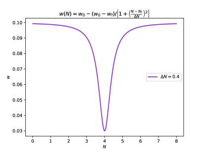
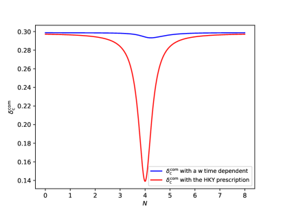
Figure 2.3: Left Panel: The equation-of-state parameter as a function of the e-fold number $N$ with $w_{0}=0.1$, $w_{\mathrm{f}}=0.03$, $\Delta N=0.4$ and $N_{\mathrm{f}}=4$. Right Panel: The PBH formation threshold, $\delta^{\mathrm{com}}_{\mathrm{c}}$, in the comoving gauge, in the case of a time-dependent equation-of-state parameter (blue line) superimposed with $\delta^{\mathrm{com}}_{\mathrm{c}}$ computed with the Harada, Kohri, Yoo (HKY) prescription, valid for a constant equation-of-state parameter.

As one may see, the PBH formation threshold computed with a time-dependent $w$ prescription is almost constant with a small decrease at $N=4$ which is expected due to the decrease of $w$ at $N\sim 4$. Interestingly, one can notice that despite the fact with the HKY prescription $\delta_{\mathrm{c}}$ decreases as $w$, if one takes into account the time-dependence of $w$ this decrease is smoothed presenting a small feature around the minimum of $w$. This effect can have important consequences for PBH formation since a higher $\delta_{\mathrm{c}}$ means smaller PBH abundances with possible consequences on the targets of future experiments.

Below, in Fig. 2.4, we show as well the dependence on $w$ and $\delta_{\mathrm{c}}$ on $\Delta N$ which is the width of variation of $w(N)$.

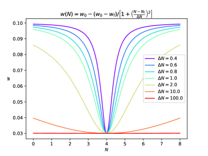
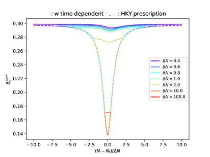
Figure 2.4: Left Panel: The equation-of-state parameter as a function of the e-fold number $N$ for different values of $\Delta N$ and with $w_{0}=0.1$, $w_{\mathrm{f}}=0.03$ and $N_{\mathrm{f}}=4$. Right Panel: The PBH formation threshold, $\delta^{\mathrm{com}}_{\mathrm{c}}$, in the comoving gauge, as a function of $(N-N_{\mathrm{f}})/\Delta N$ for different values of $\Delta N$, in the case of a time-dependent equation-of-state parameter (solid lines) superimposed with $\delta^{\mathrm{com}}_{\mathrm{c}}$ computed with the Harada, Kohri, Yoo (HKY) prescription, valid for a constant equation-of-state parameter (dashed lines).

Interestingly, as it is expected, as one increases $\Delta N$, $w(N)$ approaches a constant value and the $w$ time-dependent prescription described above approaches the one of HKY prescription valid for constant w.

2.2 Observational Constraints on PBHs

We review here the current observational constraints on the abundance of PBHs distinguishing between PBHs having been evaporated by now and PBHs that are still evaporating, following closely the recent review on the PBH constraints by Carr et al.  [29]. Concerning the extraction of the constraints presented below, one assumes a monochromatic PBH mass function (PBHs are produced with the same mass) and that PBHs form during the radiation-dominated era.

2.2.1 Evaporated PBHs

We focus here on evaporated PBHs, which have evaporated by now or they evaporate at the present time. Broadly speaking, the evaporated PBHs are black holes with masses $m_{\mathrm{PBH}}<10^{15}-10^{16}\mathrm{g}$. The constraints on the abundance of evaporated PBHs are mainly related to BBN constraints, constraints from extra-galactic $\gamma$ rays, constraints from galactic cosmic rays and constraints from CMB distortions. The summarized constraints for the evaporated PBHs are given in Fig. 2.6, taken from  [29]. In Fig. 2.6, the rescaled PBH mass function $\beta^{\prime}(M)$ at formation is plotted as a function of their mass $M$. The relevant constraint in the case of absence of Hawking evaporation (black dotted line in Fig. 2.6) are shown as well by requiring that energy density parameter of PBHs today is smaller than one, i.e. $\Omega_{\mathrm{PBH}}(M)\equiv\frac{\rho_{\mathrm{PBH}}}{\rho_{\mathrm{c}}}<1$. Below, we summarize very briefly the main physical mechanisms which give rise to the constraints of the evaporated PBHs depending on their mass.

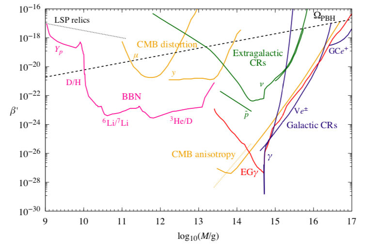
Figure 2.5: The constraints on the abundance of the evaporated PBHs as a function of their mass. With the colored lines one see the constraints on the rescaled PBH mass fraction $\beta^{\prime}(M)$ at formation due to different physical phenomena explained in the main text and assuming the validity of Hawking radiation mechanism. Otherwise, the constraints are depicted with the black dotted line where there is no Hawking radiation and are obtained by the requirement that $\Omega_{\mathrm{PBH}}(M)<1$. The allowed regions for $\beta^{\prime}(M)$ are the ones below the colored lines. Figure credited to  [29].

• BBN Constraints

  The BBN constraints on the PBH abundance are depicted with the magenta solid line in Fig. 2.5. In particular, PBHs with masses $m_{\mathrm{PBH}}<10^{9}\mathrm{g}$ can not be constrained by studying the BBN processes since they evaporate well before the time of the weak freeze-out and thus they are not tractable. For PBHs with masses $m_{\mathrm{PBH}}\approx 10^{9}-10^{10}\mathrm{g}$, Hawking radiated mesons and antinucleons induce extra interconversion of protons to neutrons increasing in this way the neutron-to-proton ratio at the time of freeze-out of the weak interaction  [134] triggering in this way an increase in the final ${}^{4}\mathrm{He}$ abundance  [135]. Regarding now the PBHs with masses $m_{\mathrm{PBH}}\approx 10^{10}-10^{12}\mathrm{g}$, long-lived high energy hadrons produced out of PBH evaporation, such as pions, kaons and nucleons remain long enough in the ambient medium and trigger dissociation processes of light elements produced during BBN  [136], reducing in this way ${}^{4}\mathrm{He}$ and increasing $\mathrm{D}$,${}^{3}\mathrm{He}$,${}^{6}\mathrm{Li}$ and ${}^{7}\mathrm{Li}$. Finally, for the PBHs with $m_{\mathrm{PBH}}\approx 10^{12}-10^{13}\mathrm{g}$, photons produced out of the particle cascade process further dissociate ${}^{4}\mathrm{He}$, increasing the abundance of light synthesized elements  [19, 137]. However, it is important to stress out that the BBN constraints carry out some uncertainties regarding the baryon-to-photon ratio, the reaction and the decay rates of the elements produced during the BBN processes. In Fig. 2.5, the most conservative constraints are depicted.

• CMB Constraints

  The CMB constraints on the PBH abundance are depicted with the brown solid line in Fig. 2.5 and as it can be seen these constraints come from CMB spectral distortions as well as from CMB anisotropies. Regarding the CMB anisotropy constraint, which is the dominant constraint on the PBH abundance for PBH masses $m_{\mathrm{PBH}}\approx 10^{13}-10^{14}\mathrm{g}$, it is related to the damping of the CMB temperature anisotropy power spectrum and a boost in the polarization at small scales. In particular, when high energy electrons, positrons and photons are injected into the baryon-photon plasma around the recombination time ($z\sim 1000$) as products of PBH evaporation they can excite and ionize the neutral hydrogen and helium leading in this way to an increase of scattering processes between CMB photons and free electrons, thereby damping the CMB temperature anisotropy and increasing the polarization at small scales  [138, 139]. Concerning now the CMB spectral distortion constraint, less stringent than the BBN constraint, which applies for the PBH mass range $m_{\mathrm{PBH}}\approx 10^{11}-10^{14}\mathrm{g}$, it is related to deviations of the CMB spectrum from the spectrum of a black body  [140, 141, 142]. Specifically, when the universe is quite young, i.e. before the emission of the CMB, the CMB achieves a black-body spectrum through photon-electron interactions, i.e. Compton and double Compton scatterings, despite of a possible high energy injection. However, as soon as the universe cools down and one is met with the decouplings of these interactions at around $z=10^{6}$, distortions from a black-body spectrum can be induced via energy injection due to PBH evaporation.

• Galactic/Extragalactic Cosmic Rays Constraints

  The extragalactic cosmic ray constraints on the PBH abundance is depicted with the green solid line in Fig. 2.5, it concerns PBHs with masses $m_{\mathrm{PBH}}\approx 10^{12}-10^{16}\mathrm{g}$ and as it can be seen, it is less stringent than all the other constraints  [143, 144, 145, 146]. With the red solid line we see the constraint as well as from the extragalactic $\gamma$ ray background (EGB) which is the dominant one for PBH masses around $m_{\mathrm{PBH}}=10^{14}\mathrm{g}$  [147, 148]. EGB is related mainly to the primary and secondary emission of photons due to Hawking evaporation of PBHs residing outside of our galaxy. The photons mostly contributing to the EGB due to PBH evaporation are mainly soft $\gamma$ ray and $X$ ray emitted photons which lead to an isotropic background different from the extragalactic cosmic ray background of other astrophysical sources. Regarding now the galactic cosmic ray constraint, it is depicted with the blue solid line in Fig. 2.5 and it is the dominant constraint for PBH masses $m_{\mathrm{PBH}}\approx 10^{15}-10^{16}\mathrm{g}$. It is related mainly to the anisotropic $\gamma$ ray background emitted from evaporated PBHs clustered inside our galactic halo  [149, 150, 23] as well as to the $e^{\pm}$  [151, 152] and $\nu/\bar{\nu}$ [153] emission due to Hawking radiation within the galactic bulge.

2.2.2 Evaporating PBHs

After having reviewed the constraints on the PBH abundance for PBHs which have evaporated by now we recap here the relevant constraints concerning PBHs which have not completed their evaporation yet. These PBHs are black holes with masses $m_{\mathrm{PBH}}>10^{15}-10^{16}\mathrm{g}$ and are considered to cluster in the galactic halo in the same way as other forms of dark matter. As in the case of the evaporated PBHs, we consider here as well that PBHs have a monochromatic mass. Historically, due to the assumption that high mass PBHs can constitute a viable candidate for cold dark matter (CDM), the constraints are given in terms of the fraction of PBHs to CDM, $f(M)$ defined as

$$f(M)\equiv\frac{\Omega_{\mathrm{PBH}}(M)}{\Omega_{\mathrm{CDM}}},$$ (2.35)

where $\Omega_{\mathrm{CDM}}=\Omega^{(0)}_{\mathrm{DM}}=0.265$  [33] and $\Omega_{\mathrm{PBH}}(M)$ is the current energy density parameter of PBHs. In the case of PBHs forming during radiation era $f(M)$ is related to $\beta^{\prime}(M)$ with the following expression  [29]

$$f(M)\simeq 10^{8}\beta^{\prime}(M)\left(\frac{M}{M_{\odot}}\right)^{-1/2}$$ (2.36)

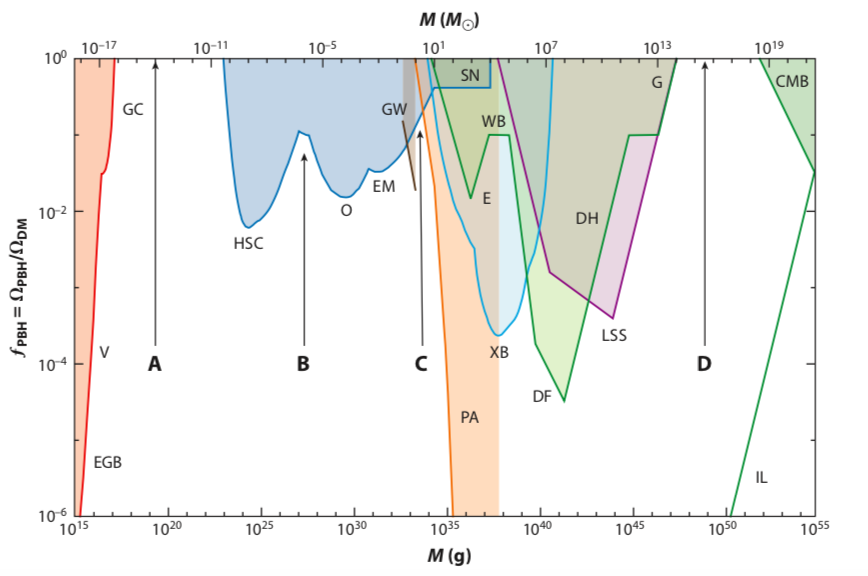
Figure 2.6: The constraints on the fraction of PBHs to cold dark matter as a function of their mass for PBHs with masses $m_{\mathrm{PBH}}>10^{15}\mathrm{g}$. With the colored regions one see the constraints on the fraction of PBHs to CDM, $f(M)$, due to different physical phenomena explained in the main text. In particular, the colored regions are the ones which are forbidden by observations. There are four possible mass windows A,B,C,D in which PBHs can have an appreciable contribution to dark matter. In the left corner of the figure one can see the constraint from the extra-galactic $\gamma$ ray background described before. Figure credited to  [27].

At this point point it is important to stress out that the majority of the constraints concerning the evaporating PBHs, presented in Fig. 2.6 are obtained by studying the observational effects that the gravitational potential of PBHs can trigger and can be divided in five large categories depending on the way PBHs induce a gravitational effect: a) gravitational lensing, b) dynamical effect, c) accretion, d) large scale structure and e) gravitational waves. Below, we recap briefly the observational constraints on the fraction of PBHs to cold dark matter depending on the gravitational effect PBHs can trigger.

• Lensing Constraints

  When between a source of light, i.e. a star, and an observer there is massive compact object, such as a PBH, one expects, as a prediction of general relativity, to observe light blending. As a consequence, the light source is observed either as an arc segment, either as a ring either as a multimple image depending on the level of alignment between the light source and the massive lensing object as well as on the mass of the lens. Regarding the PBH observational constraints due to gravitational lensing, they are related to microlensing effects in which no distortion in the shape of the light source can be seen but instead one can monitor how the amount of light received from a source change with time  [154]. Concerning now the lensing constraints on evaporating black holes, they come from microlensing events of stars observed by MACHO  [155] and EROS  [156] collaborations (EM) in the Large and Small Magellanic Clouds (LMC and SMC) which probe the fraction of the galactic halo to Massive Compact Halo Objects (MACHOs) as well as from microlensing events of stars in the galactic bulge probed by OGLE (O)  [24] . They come also from the lack of lensing events in type Ia Supernovae (SN)  [25] as well as from microlensing events of stars in M31 induced by PBHs lying in the halo regions of Milky way and M31 as observed by Subaru Hyper Suprime-Cam (HSC)  [157].

• Dynamical Constraints

  The dynamical constraints on evaporating PBHs are related to the gravitational effect a PBH can have on an astrophysical system through gravitational interactions. Up to now, many astrophysical systems have been studied. Indicatively, we mention the disruption of a white dwarf and the subsequent nuclear fusion triggered due to the passage of PBH in its vicinity  [158] as well as the disruption of a neutron star in which a PBH trapped inside it can quickly accrete the surrounding matter and destroy the star  [159, 160]. Another interesting dynamical effect of a PBH is the disruption of weakly coupled binaries of stars  [161, 162] or globular clusters  [163] of weakly coupled stars which reside in the galactic halo and which can easily disrupted from encounters of PBHs. Finally, one should mention dynamical constraints imposed to the fraction of PBHs into dark matter from disruption of ultra-faint dwarf galaxies, whose stars move faster due to gravitational interaction with PBHs  [164], from dynamical friction on PBHs  [165] as well as from the heating of stars in the galactic disk  [166] when a PBH passes through its vicinity. In Fig. 2.6 we see in the green colored regions the dominant dynamical constraints which come from wide binaries (WB), star clusters in Eridanus II (E), heating of stars in the galactic disk (DH), galaxy tidal distortions (G), halo dynamical friction and cosmic microwave dipole (CMB).

• Accretion Constraints

  The accretion constraints come from accretion of gas into PBHs and the effects of this process. Here we recap briefly the accretion effects to the CMB radiation taking place in the early universe as well as the the electromagnetic radiation emitted from accreted matter to PBHs. Regarding the accreting effects to CMB, one should take into account that the gas of baryonic nature surrounding a PBH is attracted by its gravity, starts to fall into the central region and being in this way ionised either by internal gas collisions or by the outgoing Hawking radiation. This ionisation process heats the gas filling the universe and modifies the CMB black-body spectrum, the time of photon decoupling as well as the ionisation history  [167, 168, 169, 20]. Detecting or not therefore these non-standard features on the CMB radiation one can impose limits on the PBH abundance. Concerning now the electromagnetic radiation from accreted matter to PBHs, one can impose constraints on the PBH abundance by comparing observational data and theoretical predictions of electromagnetic waves, mainly $X$ rays and radio waves, from PBH which attract and accrete their surrounding gas at present time  [170, 171, 172, 173]. In Fig. 2.6 we see in the light blue colored region the dominant accretion constraint which comes from X-ray binaries (XB) as well as in the orange colored region the accretion constraint from the Planck satellite CMB measurement (PA).

• Large Scale Structure Constraints

  The large scale structure constraints lie in the fact that the Poissonian fluctuations in the number density of randomnly distributed in space PBHs can enhance the dark matter perturbations in small scales  [3]. This enhancement of the dark matter power spectrum on small scales can have an impact on the $\mathrm{Ly\alpha}$ forest observations due to gravitational interactions of the dark matter perturbations with the baryon perturbations. Observing therefore the $\mathrm{Ly\alpha}$ absorption spectra from distant quasars and taking into account the enhacement of dark matter perturbations on small scales one can constrain the PBH abundance  [4, 174]. In addition, one can constrain the PBH abundance by suggesting PBHs as a possible solution to the tension of the observed near infrared cosmic infrared background (CIB) anisotropies  [175, 176]. The large scale structure constraints are shown in Fig. 2.6 in the purple colored region.

• Gravitational-Wave Constraints

  The gravitational-wave constraints on the PBH abundance emanate from the different ways PBHs can lead to gravitational wave (GW) production. In particular, GWs can be induced from the primordial, large curvature perurbations that must have preceded and given rise to the existence of PBHs due to second order gravitational interactions  [177, 178, 179, 180, 181, 182, 183]. In addition, GWs are also expected to be emitted by the mergers PBHs, similarly to the GWs observed through the coalescence of black hole binaries by the LIGO/VIRGO collaboration  [184, 185, 186, 187, 188, 189]. Furthermore, one expects also a gravitational-wave background due Hawking radiated gravitons  [190, 191]. Finally, one should also account for the GWs generated by PBHs themselves due to the gravitational potential they underlie  [32, 192]. By comparing therefore gravitational-wave observations with the theoretical predictions of gravitational waves associated to PBHs one can constrain the PBH abundance. In Fig. 2.6, in the brown colored region one shows the GW constraints on the PBH abundance from the early LIGO results in the range $0.5–30M_{\odot}$  [187].

2.3 Cosmological Consequences of PBHs

Given the stringent PBH constraints presented above for a wide range of PBH masses, one may deduce that PBHs are rather unlikely to constitute the totality of dark matter and be detected in the future. However, even if they do not constitute all of dark matter, their cosmological consequences are quite important since by studying them we can learn a lot about the universe state in different times of the cosmic history and probe different physical phenomena depending on the PBH mass.

Specifically, the small mass PBHs ($m_{\mathrm{PBH}}\leq 10^{15}$g) which have evaporated by now can give access to the early universe physics such as the physics of inflation and the primordial cosmological perturbations  [17] by probing the matter power spectrum on scales smaller than those of the CMB, the Big Bang Nucleosynthesis (BBN) physics  [18, 19] through Hawking evaporation and the physics of reheating  [193, 194, 30], the physics of the cosmic microwave background (CMB)  [20] through distortions of the CMB spectrum, the primordial gravitational wave physics  [21] by probing the stochastic gravitational background induced at second order in perturbation theory as well as the primordial phase transitions  [22].

Regarding the intermediate mass PBHs ($m_{\mathrm{PBH}}\sim 10^{-15}M_{\odot}$) which evaporate in our era, one can probe with them high energy astrophysical phenomena. Interestingly, as recently noticed by Carr and al.  [27] intermediate mass PBHs have been conjectured to explain the extragalactic  [143] and galactic  [149] $\gamma$-ray backgrounds through Hawking evaporation, short-period gamma-ray bursts  [195], the reionization of the pregalactic medium  [196] and antimatter in cosmic rays  [197] pointing out to an increasing interest regarding the connection of PBHs to high energy astrophysics.

Finally, the higher mass PBHs which still exist today, i.e. ($m_{\mathrm{PBH}}>10^{15}$g), can have significant cosmological consequences regarding the gravitational and the dark sector of the universe. Specifically, according to recent arguments, PBHs may indeed constitute a part or all of the dark matter [2] and they may explain the generation of large-scale structures through Poisson fluctuations [3, 4]. Furthermore, they may provide seeds for supermassive black holes in galactic nuclei [198, 6] as well as account for the progenitors of the black-hole merging events recently detected by the LIGO/VIRGO collaboration [7] through their gravitational wave (GW) emission.

Chapter 3 Inflation Theory and PBH Production from Preheating

In this chapter, we recap the basics of the theory of inflation which solves, as mentioned in Sec. 1.4, a range of fundamental problems of the Hot Big Bang theory. In particular, we recap initially the standard single-field slow-roll inflation paradigm and then we briefly present the theory of cosmological inflationary perturbations, which have seeded the PBHs studied in the context of this thesis. Finally, after reviewing the literature regarding the preheating era we discuss the PBH production in the context of single-field inflationary models theory due to metric preheating a research area to which I contributed with two scientific publications [30, 31].

Regarding my personal contribution to the above mentioned scientific publications, on the one hand, in [30] I made major contributions by performing a refined calculation for the PBH formation criterion during preheating and writing up the numerical code for the computation and the dynamical evolution of the PBH abundance. I also produced the figures of the paper, wrote up the conclusions and proof read the paper. On the other hand, in [31], my personal contribution was minor. In particular, I checked my PhD advisor’s calculation for the computation of the background equation-of-state parameter during preheating and proof read the paper. I also wrote up some conclusions regarding the effect of the inflaton’s radiative decay on PBH formation.

3.1 Inflation Theory

As discussed in Sec. 1.4, in order to account for the shortcomings of the Hot Big Bang theory one should require the existence of an early era of accelerated expansion, where $\ddot{a}>0$, which translates to the condition $p<-\rho/3$ from Eq. (1.17).

3.1.1 Single-Field Inflation

This era of negative pressure can be naturally realized in the context of single-field inflation in which a single scalar field $\phi$, the inflaton field, is minimally coupled to gravity. The action describing such a field reads as

$$\mathcal{S}_{\phi}=\int d^{4}x\mathchoice{{\hbox{$\displaystyle\sqrt{-g\,}$}\lower 0.4pt\hbox{\vrule height=4.30554pt,depth=-3.44446pt}}}{{\hbox{$\textstyle\sqrt{-g\,}$}\lower 0.4pt\hbox{\vrule height=4.30554pt,depth=-3.44446pt}}}{{\hbox{$\scriptstyle\sqrt{-g\,}$}\lower 0.4pt\hbox{\vrule height=3.01389pt,depth=-2.41113pt}}}{{\hbox{$\scriptscriptstyle\sqrt{-g\,}$}\lower 0.4pt\hbox{\vrule height=2.15277pt,depth=-1.72223pt}}}\left[\frac{1}{2}\partial_{\mu}\phi\partial^{\mu}\phi+V(\phi)\right],$$ (3.1)

where the first term in the integral is the kinetic energy of the field and the second the potential energy. The stress-energy tensor associated to the above action can be obtained from Eq. (1.14) by replacing $\mathcal{S}_{\mathrm{matter}}$ with $\mathcal{S}_{\phi}$ and is given by

$$T^{(\phi)}_{\mathrm{\mu\nu}}=\partial_{\mathrm{\mu}}\phi\partial_{\mathrm{\nu}}\phi+g_{\mathrm{\mu\nu}}\left[-\frac{1}{2}g^{\mathrm{\rho\sigma}}\partial_{\mathrm{\rho}}\phi\partial_{\mathrm{\sigma}}\phi+V(\phi)\right].$$ (3.2)

Given the fact we are working in the context of a flat FLRW background, at the background level the inflaton field $\phi$ should be homogeneous, thereby depending only on time. Thus, in this case, the energy and pressure densities of the inflaton field can be obtained from $T^{(\phi)}_{\mathrm{\mu\nu}}$ and are given by

$$\rho_{\phi}=T_{00}=\frac{\dot{\phi}^{2}}{2}+V(\phi)$$ (3.3)

$$p_{\phi}=T_{ii}=\frac{\dot{\phi}^{2}}{2}-V(\phi).$$ (3.4)

The condition then for a homogeneous scalar field to drive a period of accelerated expansion, i.e. $3p+\rho<0$, becomes

$$V(\phi)>\dot{\phi}^{2}.$$ (3.5)

The above condition ensures that in order for inflation to take place, the inflaton field should slowly roll down its potential so that its potential energy dominates over its kinetic one.

Regarding now the background dynamics of the inflaton field, it can be obtained by plugging Eq. (3.3) and Eq. (3.4) into the continuity equation Eq. (1.18). One then gets the Klein-Gordon equation for $\phi$

$$\ddot{\phi}+3H\dot{\phi}+V_{\phi}(\phi)=0$$ (3.6)

where $V_{\phi}(\phi)\equiv\mathrm{d}V(\phi)/\mathrm{d}\phi$. Concerning the Friedmann equation, it reads as

$$3M_{\scriptscriptstyle{\mathrm{Pl}}}^{2}H^{2}=V(\phi)+\frac{\dot{\phi}^{2}}{2}.$$ (3.7)

3.1.1.1 The Slow-Roll Regime

The slow-roll regime is defined when the condition Eq. (3.5) is saturated, i.e. when $V(\phi)\gg\dot{\phi}^{2}$. In such a case, one gets from Eq. (3.3) and Eq. (3.4) that $p_{\phi}\simeq-\rho_{\phi}$. In this regime, one obtains from the continuity equation 1.18 that $\rho$ is almost constant in time and from the Friedman equation one obtains that $H$ is almost constant in time too. This leads the spacetime to behave as the de Sitter one in which

$$a(t)=a_{\mathrm{ini}}e^{H(t-t_{\mathrm{ini}})}.$$ (3.8)

The de Sitter universe is equivalent with a universe dominated by a cosmological constant. See the discussion in Sec. 1.1.5. The slow-roll regime is therefore the limit in which the universe is perturbatively close to the de Sitter one. This slow-roll limit is very interesting since there is observational evidence for an almost scale invariant power spectrum on the CMB scales, as the one predicted by the slow-roll single-field inflation  [199]. One can then quantify the deviation from the de Sitter universe, by introducing the so called slow-roll parameters, upon which one can perform a perturbative expansion of the curvature power spectrum  [200, 201, 202, 203]. Although there are many possible sets of slow-roll parameters, the mostly used in the literature are the so called Hubble-flow parameters  [204, 205], $\epsilon_{n}$, defined iteratively through the following expression

$$\epsilon_{n+1}=\frac{\mathrm{d}\ln|\epsilon_{n}|}{\mathrm{d}N},$$ (3.9)

where $N$ is a time variable, called the e-fold number and it is defined as the logarithm of the scale factor, $N\equiv\ln a$. In this parametrisation for the slow-roll parameters, $\epsilon_{0}$ is defined as $\epsilon_{0}=\frac{H_{\mathrm{ini}}}{H}$, where the index $\mathrm{ini}$ denotes an initial time. In the case of a de Sitter universe, $\epsilon_{0}$ is constant and equal to $1$. Thus, in the slow-roll regime, which describes a quasi de Sitter universe, $\epsilon_{0}$ should be almost constant in time and close to $1$ and its time derivatives calculated through Eq. (3.9) should be small, a fact that makes them very useful to describe pertrurbatively the deviation from the de Sitter expansion. In the language of the slow-roll parameters one is met with the slow-roll inflation as long as $|\epsilon_{n}|\ll 1$, for all $n>0$.

3.1.2 Cosmological Perturbations in the Inflationary Epoch

As mentioned in Sec. 1, inflation constitutes the “standard theory” for the description of the early moments of the cosmic history since the primordial cosmological perturbations generated during inflation can seed the large scale structures observed today as well as the anisotropies of the relic cosmic microwave background radiation. Therefore, we recap here the theory of cosmological inflationary perturbations, which represents a cornerstone of the modern cosmology.

3.1.2.1 The Scalar-Vector-Tensor Decomposition

In order to include cosmological perturbations on the top of a homogeneous and isotropic background universe, one should go beyond homogeneity and isotropy. Thus, the most general perturbed metric which can model small perturbations of a FLRW universe can be written as  [206]

$$\mathrm{d}s^{2}=a^{2}(\eta)\left[-(1+2A)\mathrm{d}\eta^{2}+2B_{i}\mathrm{d}x^{i}\mathrm{d}\eta+\left(\gamma_{ij}+h_{ij}\right)\mathrm{d}x^{i}\mathrm{d}x^{j}\right],$$ (3.10)

where $A$, $B_{i}$ and $h_{ij}$ are functions of space and time describing the deviation from a homogeneous and isotropic universe. $\gamma_{ij}$ is the spatial part of the background metric. In our case, since we consider a flat FLRW background universe, $\gamma_{ij}=\delta_{ij}$.

In order now to extract the dynamics of the cosmological perturbations it is very useful to decompose them into scalar, vector and tensor components, thus the name Scalar-Vector-Tensor (SVT) decomposition  [207]. In particular, any vector field, $B_{i}$ can be decomposed into the divergence of a scalar field, $B$, and to a vector field , $\bar{B}_{i}$, with vanishing divergence , that is

$$B_{i}=\partial_{i}B+\bar{B}_{i},\quad\mathrm{with}\quad\partial^{i}\bar{B}_{i}=0.$$ (3.11)

In the same way, any tensor field, $h_{ij}$, can be decomposed into

$$h_{ij}=-2\psi\gamma_{ij}+2\partial_{i}\partial_{j}E+2\partial_{(i}\bar{E}_{j)}+2\bar{E}_{ij},\quad\mathrm{with}\quad\partial_{i}\bar{E}^{ij}=0\quad\mathrm{and}\quad\bar{E}^{i}_{i}=0.$$ (3.12)

The vector perturbations are rapidly supressed during the inflationary stage and therefore they are usually disregarded  [208]. Scalar and tensor perturbations are instead studied with a lot of attention. Focusing then for the moment on scalar perturbations at linear order and making use of the SVT decomposition described above, the metric in Eq. (3.10) reads as

$$\mathrm{d}s^{2}=a^{2}(\eta)\left\{-(1+2A)\mathrm{d}\eta^{2}+2\partial_{i}B\mathrm{d}x^{i}\mathrm{d}\eta+\left[(1-2\psi)\delta_{ij}+2\partial_{i}\partial_{j}E\right]\mathrm{d}x^{i}\mathrm{d}x^{j}\right\},$$ (3.13)

where we have replaced $\gamma_{ij}=\delta_{ij}$ since as mentioned in Sec. 1.3 the observed negligible spatial curvature favors a flat FLRW background universe.

3.1.2.2 The Gauge Issue

The study of cosmological perturbations lies in comparing the differences of physical quantities between a background spacetime (here FLRW metric) which is homogeneous and isotropic and the physical spacetime which does not obey necessarily to the cosmological principle. Thus, in order to compute the cosmological perturbations of a physical quantity one should compare the value it assumes at the unperturbed background spacetime with its value at the perturbed one at the same spacetime point. Since these values live in different spacetime geometries, it is important to find a correspondence that links the same point on the two different spacetimes. This correspondence is called gauge choice and fixing a gauge is equivalent to choosing a threading into lines, corresponding to fixed spatial coordinates, and a slicing into hypersurfaces, corresponding to fixed time.

Let us consider a generic infinitesimal coordinate/gauge transformation which reads

$$x^{\mathrm{\mu}}\rightarrow\tilde{x}^{\mathrm{\mu}}=x^{\mathrm{\mu}}+\xi^{\mathrm{\mu}},$$ (3.14)

where $\xi^{\mathrm{\mu}}=(\xi^{0},\xi^{i})$ is an arbitrary four-vector whose components $\xi^{0}$ and $\xi^{i}$ depend on space and time. As discussed in the previous section any vector field $\xi^{i}$ can be decomposed into the divergence of a scalar field, $\xi$, and to a vector field , $\xi^{i}_{\mathrm{tr}}$, with vanishing divergence ($\xi^{i}_{\mathrm{tr},i}=0$), i.e. $\xi^{i}=\gamma^{ij}\xi_{,j}+\xi^{i}_{\mathrm{tr}}$, where the comma stands for the covariant derivative with respect to the background space coordinates. Therefore, taking into account only the functions $\xi^{0}$ and $\xi$ which preserve the scalar nature of the metric perturbations one can write Eq. (3.14) as

$$\tilde{x}^{0}=x^{0}+\xi^{0}(x^{0},x^{i}),\quad\bar{x}^{i}=x^{i}+\gamma^{ij}\xi_{,j}(x^{0},x^{i}).$$ (3.15)

Under this gauge transformation the scalar perturbations $A$, $B$, $\psi$ and $E$ transform like  [206]

$$\tilde{A}=A-\frac{a^{\prime}}{a}\xi^{0}-\xi^{0\prime},\quad\tilde{\psi}=\psi+\frac{a^{\prime}}{a}\xi^{0},\quad\tilde{B}=B+\xi^{0}-\xi^{\prime},\quad\tilde{E}=E-\xi,$$ (3.16)

where the prime denotes derivative with respect to the conformal time $\eta$ defined in Sec. 1.1.1.

The issue which is risen now with the gauge choice is that there is not a preferred gauge. This is equivalent to the fact that there is not a unique choice of the functions $A$, $B$, $\psi$ and $E$  [207]. Therefore, to address this issue one can make two choices:

• Make all the calculations in terms of gauge invariant quantities

• Make a gauge choice and perform the calculations in that gauge

Both of these choices have advantages and disadvantages. Making a specific gauge choice may render the computations technically simpler but at the same time it can potentially introduce gauge artifacts. On the other hand, performing a gauge-invariant computation, maybe more technically involved, gives the advantage to work with only physical quantities. One can construct gauge-invariant quantities by taking combinations of $A$, $B$, $\psi$ and $E$. The simplest gauge-invariant quantities constructed from linear combinations of $A$, $B$, $\psi$ and $E$ that describe the gravitational sector are the so called Bardeen potentials and are defined as follows  [207]:

$$\Phi\equiv A+\frac{1}{a}\left[\left(B-E^{\prime}\right)a\right]^{\prime},\quad\Psi\equiv\psi-\frac{a^{\prime}}{a}(B-E^{\prime}).$$ (3.17)

In the absence of anisotropic stress, i.e. in the absence of non diagonal space-space components in the stress-energy tensor, one can prove that $\Phi=\Psi$. Regarding the matter sector, one can construct a gauge-invariant fluctuation for the scalar field $\phi$ as follows

$$\delta\phi^{(\mathrm{gi})}(\eta,{\bm{x}})\equiv\delta\phi+\phi^{\prime}(B-E^{\prime}).$$ (3.18)

In the same manner, one can define gauge-invariant scalar fluctuations like $\delta\rho^{(\mathrm{gi})}$ and $\delta p^{(\mathrm{gi})}$. In particular, given a scalar quantity $f$ one can define a gauge-invariant fluctuation $\delta f^{(\mathrm{gi})}$ as

$$\delta f^{(\mathrm{gi})}\equiv\delta f+f^{\prime}(B-E^{\prime}).$$ (3.19)

Here it is important to know that the construction of $\delta f^{(\mathrm{gi})}$ present in Eq. (3.19) is the one mostly used in the literature but in fact there are infinitely more possibilities one can construct a gauge-invariant scalar fluctuation.

3.1.2.3 The Perturbed Einstein’s equations in a gauge-invariant form

The matter and metric (gravitational) fluctuations are related to each other through the Einstein’s equations. Specifically, working with gauge-invariant quantities one can show that in the absence of anisotropic stress, i.e. $\Phi=\Psi$, the perturbed Einstein’s equations $\delta G^{\mathrm{(gi)}}_{\mathrm{\mu\nu}}=8\pi\delta T^{\mathrm{(gi)}}_{\mathrm{\mu\nu}}$ after a straightforward but tedious calculation take the following form  [206]

$$\nabla^{2}\Phi-3\mathcal{H}\Phi^{\prime}-3\mathcal{H}^{2}\Phi = \frac{a^{2}}{2M_{\scriptscriptstyle{\mathrm{Pl}}}^{2}}\delta T^{\mathrm{(gi)}0}_{0},$$ (3.22)

$$\partial_{i}(\Phi^{\prime}+\mathcal{H}\Phi) = \frac{a^{2}}{2M_{\scriptscriptstyle{\mathrm{Pl}}}^{2}}\delta T^{\mathrm{(gi)}0}_{i},$$ (3.23)

$$\left[\Phi^{\prime\prime}+3\mathcal{H}\Phi^{\prime}+(2\mathcal{H}^{\prime}+\mathcal{H}^{2})\Phi\right]\delta^{i}_{j} = -\frac{a^{2}}{2M_{\scriptscriptstyle{\mathrm{Pl}}}^{2}}\delta T^{\mathrm{(gi)}i}_{j}\,.$$ (3.24)

Working therefore with the stress-energy tensor of the inflaton field, Eq. (3.2), one can find that the perturbed stress-energy tensor reads as  [206]

$$\delta T^{\mathrm{(gi)}0}_{0}=a^{-2}\left(-\phi^{\prime 2}\Phi+\phi^{\prime}\delta\phi^{\mathrm{(gi)\prime}}+V_{\phi}(\phi)a^{2}\delta\phi^{\mathrm{(gi)}}\right)$$ (3.25)

$$\delta T^{\mathrm{(gi)}0}_{i}=a^{-2}\phi^{\prime}\partial_{i}\delta\phi^{\mathrm{(gi)}}$$

$$\delta T^{\mathrm{(gi)i}}_{j}=a^{-2}\left(\phi^{\prime 2}\Phi-\phi^{\prime}\delta\phi^{\mathrm{(gi)\prime}}+V_{\phi}(\phi)a^{2}\delta\phi^{\mathrm{(gi)}}\right)\delta^{i}_{j}$$

Consequently, plugging Eq. (3.25) into Eq. (3.22) one obtains that

$$\nabla^{2}\Phi-3\mathcal{H}\Phi^{\prime}-3\mathcal{H}^{2}\Phi = \frac{1}{2M_{\scriptscriptstyle{\mathrm{Pl}}}^{2}}\left(-\phi^{\prime 2}\Phi+\phi^{\prime}\delta\phi^{\mathrm{(gi)\prime}}+V_{,\phi}(\phi)a^{2}\delta\phi^{\mathrm{(gi)}}\right),$$ (3.26)

$$(\Phi^{\prime}+\mathcal{H}\Phi) = \frac{1}{2M_{\scriptscriptstyle{\mathrm{Pl}}}^{2}}\phi^{\prime}\delta\phi^{\mathrm{(gi)}},$$ (3.27)

$$\Phi^{\prime\prime}+3\mathcal{H}\Phi^{\prime}+(2\mathcal{H}^{\prime}+\mathcal{H}^{2})\Phi = -\frac{1}{2M_{\scriptscriptstyle{\mathrm{Pl}}}^{2}}\left(\phi^{\prime 2}\Phi-\phi^{\prime}\delta\phi^{\mathrm{(gi)\prime}}+V_{,\phi}(\phi)a^{2}\delta\phi^{\mathrm{(gi)}}\right).$$ (3.28)

At this point, one can extract an equation for the dynamics of $\Phi$, which describes the gravitational sector. In particular, by substracting Eq. (3.26) from Eq. (3.28), using Eq. (3.27) to express $\delta\phi^{\mathrm{(gi)}}$ as a function of $\Phi$ and $\Phi^{\prime}$ as well as the Klein-Gordon equation Eq. (3.6), one obtains that

$$\Phi^{\prime\prime}+2\left(\mathcal{H}-\frac{\phi^{\prime\prime}}{\phi^{\prime}}\right)\Phi^{\prime}-\nabla^{2}\Phi+2\left(\mathcal{H}^{\prime}-\mathcal{H}\frac{\phi^{\prime\prime}}{\phi^{\prime}}\right)\Phi=0.$$ (3.29)

3.1.2.4 The Curvature Perturbation

As we saw previously, the matter perturbations, here the scalar field perturbations $\delta\phi^{\mathrm{(gi)}}$, source metric perturbations $\Phi$ through the Einstein equations, which can be translated to perturbations of the curvature of the spacetime. These perturbations of the curvature of spacetime are of great importance since these are the ones which can explain through the theory of inflation the large scale structure and the CMB anisotropies. In this paragraph, we introduce the curvature perturbation in two gauges, most studied in the literature and then we construct gauge-invariant curvature perturbations starting from these two gauges  [209].

• The comoving curvature perturbation

  The function $\psi$, appearing in the spatial part of the perturbed metric is related to the intrinsic curvature of hypersuperfaces of constant time. In the case of a flat FLRW background one can show that the spatial Ricci scalar, ${}^{(3)}R$, defined as ${}^{(3)}R\equiv\gamma^{ij}R_{ij}$, is related to $\psi$ as follows

  $${}^{(3)}R=\frac{4}{a^{2}}\nabla^{2}\psi.$$ (3.30)

  The comoving curvature perturbation, $\mathcal{R}$, is defined as the metric perturbation $\psi$ in the comoving slicing, which is the slicing of free-falling comoving observers for which the expansion is isotropic. In this gauge, there is no energy flux measured by the comoving observers, i.e. $T^{0}_{i}=0$. Therefore, $\mathcal{R}$ is defined as

  $$\mathcal{R}\equiv\psi|_{T^{0}_{i}=0}.$$ (3.31)

  One then can express $\mathcal{R}$ in a general gauge through a gauge transformation on constant time surfaces $\eta\rightarrow\eta+\delta\eta$. Under this transformation, $\psi$ transforms according to Eq. (3.15) with $\xi^{0}=\delta\eta$ as follows

  $$\psi\rightarrow\tilde{\psi}=\psi+\mathcal{H}\delta\eta.$$ (3.32)

  In the comoving gauge, $T^{\mathrm{0}}_{i}=0$ and given the fact that at the background level ${}^{(0)}T^{0}_{i}=0$ as can be checked from Eq. (3.2), and that $\delta T^{\mathrm{(gi)}0}_{i}\propto\partial_{i}\delta\phi\phi^{\prime}$ as can be seen from Eq. (3.25), one gets that the fluctuation for the scalar field $\phi$ in the comoving gauge, $\delta\phi_{\mathrm{com}}$ vanishes, i.e. $\delta\phi_{\mathrm{com}}=0$. To proceed now further and extract the expression for $\mathcal{R}$ in a generic gauge we should identify how a scalar fluctuation, like $\delta\phi$, transforms under a gauge transformation.

  Let then $f$ be a scalar quantity and consider the generic coordinate transformation given by Eq. (3.14). Since $f$ is a scalar quantity, its value at a given physical point is the same in all coordinate systems. Thus, $\tilde{f}(\tilde{x}^{\mathrm{\mu}})=f(x^{\mathrm{\mu}})$. In addition, one has as well for the unperturbed background that $f_{0}(x^{\mathrm{\mu}})=\tilde{f}_{0}(x^{\mathrm{\mu}})$ where the index $0$ denotes background quantities. Consequently, one can deduce how the scalar fluctuation $\delta f(x^{\mathrm{\mu}})\equiv f(x^{\mathrm{\mu}})-f_{0}(x^{\mathrm{\mu}})$ transforms under a generic coordinate transformation. In particular, one obtains that

  $$\begin{split}\tilde{\delta f}(\tilde{x}^{\mathrm{\mu}})&=\tilde{f}(\tilde{x}^{\mathrm{\mu}})-\tilde{f}_{0}(\tilde{x}^{\mathrm{\mu}})\\ &=f(x^{\mathrm{\mu}})-f_{0}(\tilde{x}^{\mathrm{\mu}})\\ &=f(\tilde{x}^{\mathrm{\mu}})-\delta x^{\mathrm{\mu}}\frac{\partial f}{\partial x^{\mathrm{\mu}}}(\tilde{x}^{\mathrm{\mu}})-f_{0}(\tilde{x}^{\mathrm{\mu}})\\ &\simeq\delta f(\tilde{x}^{\mathrm{\mu}})-\delta x^{\mathrm{\mu}}\frac{\partial}{\partial x^{\mathrm{\mu}}}\left(f_{0}(\tilde{x}^{\mathrm{\mu}})+\delta f(\tilde{x}^{\mathrm{\mu}})\right),\end{split}$$ (3.33)

  where in the last equality we expanded up to first order the function $f(\tilde{x}^{\mathrm{\mu}})$. Then, given the fact that for a homogeneous and isotropic scalar field the background function $f_{0}$ depends only on time and considering up to first order contributions, $\tilde{\delta f}(\tilde{x}^{\mathrm{\mu}})$ reads as

  $$\tilde{\delta f}(\tilde{x}^{\mathrm{\mu}})=\delta f(x^{\mathrm{\mu}})-f^{\prime}_{0}\delta\eta.$$ (3.34)

  Thus, following the derivation presented above, $\delta\phi$ will transform as $\delta\phi\rightarrow\delta\phi-\phi^{\prime}\delta\eta$ and therefore one gets for a transformation on constant time hypersurfaces that

  $$\delta\phi\rightarrow\delta\phi_{\mathrm{com}}=\delta\phi-\phi^{\prime}\delta\eta=0\Leftrightarrow\delta\eta=\frac{\delta\phi}{\phi^{\prime}}.$$ (3.35)

  Consequently, given Eq. (3.32) and Eq. (3.35), the comoving curvature perturbation, $\mathcal{R}$ can be defined in a generic gauge as

  $$\mathcal{R}\equiv\psi+\mathcal{H}\frac{\delta\phi}{\phi^{\prime}}.$$ (3.36)

  At this point it is important to point out that the above quantity is gauge-invariant by construction. Thus, $\mathcal{R}$ can be viewed as the gravitational potential on hypersurfaces where $\delta\phi=0$

  $$\mathcal{R}=\psi|_{\delta\phi=0}.$$

  Let us also stress out here the usefulness of the comoving curvature perturbation given its constancy on large scales  [210]. It can be used then to propagate the inflationary power spectrum from the end of inflation to the post-inflationary era.

• The uniform energy density curvature perturbation

  In the same way, we can define the uniform energy density curvature perturbation, $\zeta$ by considering a slicing with $\delta\rho=0$. Thus, $\zeta$ is defined as

  $$\zeta\equiv\psi|_{\delta\rho=0}.$$ (3.37)

  For a transformation on constant time hypersurfaces, given the fact that $\delta\rho$ being a scalar fluctuation it transforms as $\delta\rho\rightarrow\delta\rho-\rho^{\prime}\delta\eta$, one can find, following the same reasoning as in the case of the comoving slicing, that in the uniform energy density slicing $\delta\eta=\frac{\delta\rho}{\rho^{\prime}}$. Therefore, in a generic gauge $\zeta$ is defined as

  $$\zeta\equiv\psi+\mathcal{H}\frac{\delta\rho}{\rho^{\prime}}$$ (3.38)

  and it is by construction a gauge-invariant quantity. It is worth to mentioning here that it can be proved that, on superhorizon scales, i.e. $k\ll aH$, the curvature perturbation on the uniform energy density gauge, $\zeta$, is equal to the comoving curvature perturbation, $\cal{R}$  [209].

3.1.2.5 The equation of motion for the scalar perturbations

In Sec. 3.1.2.2, we have introduced the Bardeen potentials $\Phi$ and $\Psi$, which are equal in the case of a vanishing anisotropic stress and which describe the gravitational sector as well as the gauge-invariant inflaton perturbation $\delta\phi^{\mathrm{(gi)}}$ which describes the matter sector. These gauge-invariant quantities are related to each through the Einstein equations as we saw in Sec. 3.1.2.3. This implies that one can construct a gauge-invariant quantity which describes in a unique way the scalar sector, i.e. the gravitational and the matter one. For this reason, the Mukhanov-Sasaki variable is introduced, which is a combination of the Bardeen potential and the gauge-invariant inflaton perturbation $\delta\phi^{\mathrm{(gi)}}$ and it is defined as  [211, 212]

$$v(\eta,{\bm{x}})=a\left(\delta\phi^{\mathrm{(gi)}}+\phi^{\prime}\frac{\Phi}{\mathcal{H}}\right).$$ (3.39)

At this point, it is useful to mention that the Mukhanov-Sasaki variable is related to the comoving curvature perturbation $\cal{R}$ as follows

$$v=\frac{a\phi^{\prime}}{\mathcal{H}}\cal{R},$$ (3.40)

where the last equation is a gauge-invariant equation constructed by starting from the Newtonian gauge in which $E=B=0$ and $\Psi=\psi$ and having taken into account that $\Phi=\Psi$ in the absence of anisotropic stress.

To extract the equation of motion for $u(\eta,{\bm{x}})$, one should write the total action of the system at hand, which is the sum of the action of the gravitational sector, i.e. the Einstein-Hilbert action 1.9, plus the action of the matter sector which is the inflaton scalar field action 3.1 and write the respective Laplace equation for the Mukhanov-Sasaki equation. To do so, one expands the action of the system up to second order in perturbations to obtain after a rather lengthy calculation that  [206]

$$^{(2)}\delta\mathcal{S}=\frac{1}{2}\int\mathrm{d}^{4}x\left[v^{\prime 2}-\delta^{ij}\partial_{i}v\partial_{j}v+\frac{\left(a\mathchoice{{\hbox{$\displaystyle\sqrt{\epsilon_{1}\,}$}\lower 0.4pt\hbox{\vrule height=4.30554pt,depth=-3.44446pt}}}{{\hbox{$\textstyle\sqrt{\epsilon_{1}\,}$}\lower 0.4pt\hbox{\vrule height=4.30554pt,depth=-3.44446pt}}}{{\hbox{$\scriptstyle\sqrt{\epsilon_{1}\,}$}\lower 0.4pt\hbox{\vrule height=3.01389pt,depth=-2.41113pt}}}{{\hbox{$\scriptscriptstyle\sqrt{\epsilon_{1}\,}$}\lower 0.4pt\hbox{\vrule height=2.15277pt,depth=-1.72223pt}}}\right)^{\prime\prime}}{a\mathchoice{{\hbox{$\displaystyle\sqrt{\epsilon_{1}\,}$}\lower 0.4pt\hbox{\vrule height=4.30554pt,depth=-3.44446pt}}}{{\hbox{$\textstyle\sqrt{\epsilon_{1}\,}$}\lower 0.4pt\hbox{\vrule height=4.30554pt,depth=-3.44446pt}}}{{\hbox{$\scriptstyle\sqrt{\epsilon_{1}\,}$}\lower 0.4pt\hbox{\vrule height=3.01389pt,depth=-2.41113pt}}}{{\hbox{$\scriptscriptstyle\sqrt{\epsilon_{1}\,}$}\lower 0.4pt\hbox{\vrule height=2.15277pt,depth=-1.72223pt}}}}u^{2}\right],$$ (3.41)

where $\epsilon_{1}$ is the first slow-roll parameter defined through the recursive Eq. (3.9). Then, the next step, is to write the action in terms of the the Fourier modes of $v(\eta,{\bm{x}})$, given the fact that in the context of a linear theory each mode evolves independently. Consequently, expanding $v(\eta,{\bm{x}})$ in Fourier modes we have that

$$v(\eta,{\bm{x}})=\frac{1}{\left(2\pi\right)^{3/2}}\int_{\mathbb{R}}\mathrm{d}^{3}{\bm{k}}v_{\bm{k}}(\eta)e^{i{\bm{k}}\cdot{\bm{x}}},$$ (3.42)

with $v_{-{\bm{k}}}=v^{*}_{\bm{k}}$ since $v(\eta,{\bm{x}})$ is real. Then, inserting Eq. (3.42) into Eq. (3.41) one gets that  [206]

$$^{(2)}\delta\mathcal{S}=\int\mathrm{d}\eta\int_{\mathbb{R}^{+}\times\mathbb{R}^{2}}\mathrm{d}^{3}{\bm{k}}\Bigg{\{}v^{\prime}_{\bm{k}}v^{*\prime}_{\bm{k}}+v_{\bm{k}}v^{*}_{\bm{k}}\left[\frac{\left(a\mathchoice{{\hbox{$\displaystyle\sqrt{\epsilon_{1}\,}$}\lower 0.4pt\hbox{\vrule height=4.30554pt,depth=-3.44446pt}}}{{\hbox{$\textstyle\sqrt{\epsilon_{1}\,}$}\lower 0.4pt\hbox{\vrule height=4.30554pt,depth=-3.44446pt}}}{{\hbox{$\scriptstyle\sqrt{\epsilon_{1}\,}$}\lower 0.4pt\hbox{\vrule height=3.01389pt,depth=-2.41113pt}}}{{\hbox{$\scriptscriptstyle\sqrt{\epsilon_{1}\,}$}\lower 0.4pt\hbox{\vrule height=2.15277pt,depth=-1.72223pt}}}\right)^{\prime\prime}}{a\mathchoice{{\hbox{$\displaystyle\sqrt{\epsilon_{1}\,}$}\lower 0.4pt\hbox{\vrule height=4.30554pt,depth=-3.44446pt}}}{{\hbox{$\textstyle\sqrt{\epsilon_{1}\,}$}\lower 0.4pt\hbox{\vrule height=4.30554pt,depth=-3.44446pt}}}{{\hbox{$\scriptstyle\sqrt{\epsilon_{1}\,}$}\lower 0.4pt\hbox{\vrule height=3.01389pt,depth=-2.41113pt}}}{{\hbox{$\scriptscriptstyle\sqrt{\epsilon_{1}\,}$}\lower 0.4pt\hbox{\vrule height=2.15277pt,depth=-1.72223pt}}}}-k^{2}\right]\Bigg{\}},$$ (3.43)

where we integrate over the half of the Fourier space given the redundancy $v_{-{\bm{k}}}=v^{*}_{\bm{k}}$. Therefore, the Lagrangian density in Fourier space reads as

$$\mathcal{L}\equiv\int_{\mathbb{R}^{+}\times\mathbb{R}^{2}}\mathrm{d}^{3}{\bm{k}}\Bigg{\{}v^{\prime}_{\bm{k}}v^{*\prime}_{\bm{k}}+v_{\bm{k}}v^{*}_{\bm{k}}\left[\frac{\left(a\mathchoice{{\hbox{$\displaystyle\sqrt{\epsilon_{1}\,}$}\lower 0.4pt\hbox{\vrule height=4.30554pt,depth=-3.44446pt}}}{{\hbox{$\textstyle\sqrt{\epsilon_{1}\,}$}\lower 0.4pt\hbox{\vrule height=4.30554pt,depth=-3.44446pt}}}{{\hbox{$\scriptstyle\sqrt{\epsilon_{1}\,}$}\lower 0.4pt\hbox{\vrule height=3.01389pt,depth=-2.41113pt}}}{{\hbox{$\scriptscriptstyle\sqrt{\epsilon_{1}\,}$}\lower 0.4pt\hbox{\vrule height=2.15277pt,depth=-1.72223pt}}}\right)^{\prime\prime}}{a\mathchoice{{\hbox{$\displaystyle\sqrt{\epsilon_{1}\,}$}\lower 0.4pt\hbox{\vrule height=4.30554pt,depth=-3.44446pt}}}{{\hbox{$\textstyle\sqrt{\epsilon_{1}\,}$}\lower 0.4pt\hbox{\vrule height=4.30554pt,depth=-3.44446pt}}}{{\hbox{$\scriptstyle\sqrt{\epsilon_{1}\,}$}\lower 0.4pt\hbox{\vrule height=3.01389pt,depth=-2.41113pt}}}{{\hbox{$\scriptscriptstyle\sqrt{\epsilon_{1}\,}$}\lower 0.4pt\hbox{\vrule height=2.15277pt,depth=-1.72223pt}}}}-k^{2}\right]\Bigg{\}},$$ (3.44)

with the conjugate momentum $p_{\bm{k}}$ being defined as

$$p_{\bm{k}}\equiv\frac{\delta\mathcal{L}}{\delta v^{*\prime}_{\bm{k}}}=v^{\prime}_{\bm{k}}.$$ (3.45)

Thus, the Laplace equation, which comes out of minimizing the action ${}^{(2)}\delta\mathcal{S}$, reads as $\partial\mathcal{L}/\partial v^{*}_{\bm{k}}=\partial_{\eta}\left(\partial\mathcal{L}/\partial p^{*}_{\bm{k}}\right)$ and leads to the equation of motion for the Mukhanov-Sasaki variable which is given by

$$v^{\prime\prime}_{\bm{k}}+\left[k^{2}-\frac{\left(a\mathchoice{{\hbox{$\displaystyle\sqrt{\epsilon_{1}\,}$}\lower 0.4pt\hbox{\vrule height=4.30554pt,depth=-3.44446pt}}}{{\hbox{$\textstyle\sqrt{\epsilon_{1}\,}$}\lower 0.4pt\hbox{\vrule height=4.30554pt,depth=-3.44446pt}}}{{\hbox{$\scriptstyle\sqrt{\epsilon_{1}\,}$}\lower 0.4pt\hbox{\vrule height=3.01389pt,depth=-2.41113pt}}}{{\hbox{$\scriptscriptstyle\sqrt{\epsilon_{1}\,}$}\lower 0.4pt\hbox{\vrule height=2.15277pt,depth=-1.72223pt}}}\right)^{\prime\prime}}{a\mathchoice{{\hbox{$\displaystyle\sqrt{\epsilon_{1}\,}$}\lower 0.4pt\hbox{\vrule height=4.30554pt,depth=-3.44446pt}}}{{\hbox{$\textstyle\sqrt{\epsilon_{1}\,}$}\lower 0.4pt\hbox{\vrule height=4.30554pt,depth=-3.44446pt}}}{{\hbox{$\scriptstyle\sqrt{\epsilon_{1}\,}$}\lower 0.4pt\hbox{\vrule height=3.01389pt,depth=-2.41113pt}}}{{\hbox{$\scriptscriptstyle\sqrt{\epsilon_{1}\,}$}\lower 0.4pt\hbox{\vrule height=2.15277pt,depth=-1.72223pt}}}}\right]v_{\bm{k}}=0.$$ (3.46)

From the above equation, one clearly sees that each mode ${\bm{k}}$ behaves as a parametric oscillator with a time-dependent frequency $\omega(\eta,{\bm{k}})$ expressed as

$$\omega^{2}(\eta,{\bm{k}})=k^{2}-\frac{\left(a\mathchoice{{\hbox{$\displaystyle\sqrt{\epsilon_{1}\,}$}\lower 0.4pt\hbox{\vrule height=4.30554pt,depth=-3.44446pt}}}{{\hbox{$\textstyle\sqrt{\epsilon_{1}\,}$}\lower 0.4pt\hbox{\vrule height=4.30554pt,depth=-3.44446pt}}}{{\hbox{$\scriptstyle\sqrt{\epsilon_{1}\,}$}\lower 0.4pt\hbox{\vrule height=3.01389pt,depth=-2.41113pt}}}{{\hbox{$\scriptscriptstyle\sqrt{\epsilon_{1}\,}$}\lower 0.4pt\hbox{\vrule height=2.15277pt,depth=-1.72223pt}}}\right)^{\prime\prime}}{a\mathchoice{{\hbox{$\displaystyle\sqrt{\epsilon_{1}\,}$}\lower 0.4pt\hbox{\vrule height=4.30554pt,depth=-3.44446pt}}}{{\hbox{$\textstyle\sqrt{\epsilon_{1}\,}$}\lower 0.4pt\hbox{\vrule height=4.30554pt,depth=-3.44446pt}}}{{\hbox{$\scriptstyle\sqrt{\epsilon_{1}\,}$}\lower 0.4pt\hbox{\vrule height=3.01389pt,depth=-2.41113pt}}}{{\hbox{$\scriptscriptstyle\sqrt{\epsilon_{1}\,}$}\lower 0.4pt\hbox{\vrule height=2.15277pt,depth=-1.72223pt}}}}.$$ (3.47)

As one can see, the frequency $\omega(\eta,{\bm{k}})$ depends on the scale factor and its derivatives. Thus, different inflationary potentials, which lead to different dynamics of the scale factor through the Friedman equation, lead to different dynamics of $\omega(\eta,{\bm{k}})$ and subsequently to different dynamics of $v_{\bm{k}}(\eta)$.

3.2 PBHs from the Preheating Instability

Having introduced before the fundamentals of the inflationary theory and the theory of cosmological perturbations we study here the period of preheating after the end of inflation and the possibility of PBH production during this early era of the cosmic history. Initially, we make a brief introduction of preheating reviewing the relevant literature on the field and then we discuss the PBH production from metric preheating in the context of single-field inflationary models as discussed in the relevant research works completed within my PhD  [30, 31].

3.2.1 Preheating

When inflation ends, i.e. when the kinetic and the potential energy of the inflaton field become comparable, the inflaton field approaches a local minimum of its potential, which can be approximated in most cases by a quadratic potential of the form $V=m^{2}\phi^{2}/2$, where $m$ is a mass scale representing the curvature of the inflationary potential at its minimum. Then, when the inflaton reaches the minimum of its potential, it starts oscillating like $\phi\propto a^{-3/2}\sin(mt)$ driving a decelerated expansion in which the universe’s thermal state behaves on average as a matter-domination state with $\langle\rho\rangle\propto a^{-3}$  [52], where $\langle\rangle$ denotes an average over the inflaton’s oscillations. This oscillatory era is quoted in the literature as preheating.

These rapid oscillations can parametrically amplify the quantum fields present during preheating both at the background and at the perturbative level  [54, 55]. However, the consideration described above does not take into account the coupling of the inflaton to other degrees of freedom, which is necessary to ensure the transition to the radiation era, i.e. the Hot Big Bang phase of the universe. For this reason, more realistic preheating models consider these couplings as well. Below, we recap briefly how one can potentially couple the inflaton field with other degrees of freedom and generate a parametrically resonant amplification regime for the fields present during preheating.

3.2.1.1 The background

At the background level, one can introduce the coupling of the inflaton field with other degrees of freedom by adding an extra friction term “$\Gamma\dot{\phi}$” - where $\Gamma$ is a decay rate - in the Klein-Gordon equation 3.6, which basically accounts for the decay of the inflaton to a perfect fluid, usually radiation. Initially, $H\gg\Gamma$ and the effect of the inflaton’s decay is negligible. As the universe expands, $H$ decreases and at some point $H\sim\Gamma$, which is the time when the decay of the inflaton starts taking place. The decay rate depends on the specifics of the model considered, i.e. the coupling of the inflaton with the perfect fluid as well as the relevant mass scales and can be calculated within perturbation theory. This perturbative approach, initially studied in the context of reheating after inflation by  [213, 214], has however some limitations. It can describe energy transfers due to individual decays of the inflaton to other degrees of freedom and it is efficient only for the last stages of reheating when the energy transfer to the inflaton’s decay products is small compared to the very efficient energy transfer taken place during the very rapid coherent oscillations of the inflaton around its minimum during the early stage of preheating  [54, 55].

Therefore, one should consider non perturbative effects when considering the background behavior during the oscillatory phase of preheating. To illustrate this with an example, one can couple the inflaton field $\phi$ with another scalar field $\chi$ with an interaction Lagrangian $\mathcal{L}_{\mathrm{int}}=-g^{2}\phi^{2}\chi^{2}/2$ where $g$ is a dimensionless coupling constant. Then, the total Lagrangian of the system can be written as $\mathcal{L}=\mathcal{L}_{\mathrm{\phi}}+\mathcal{L}_{\mathrm{\chi}}+\mathcal{L}_{\mathrm{int}}$, with $\mathcal{L}_{\mathrm{\phi}}=-m^{2}\phi^{2}/2+\dot{\phi}^{2}/2$, $\mathcal{L}_{\mathrm{\chi}}=-m^{2}_{\mathrm{\chi}}\chi^{2}/2+\dot{\chi}^{2}/2$ and the equation of motion for the Fourier mode $\chi_{\bm{k}}$ can be written as

$$\ddot{\chi}_{\bm{k}}+3H\dot{\chi}_{\bm{k}}+\left[\frac{k^{2}}{a^{2}(t)}+m_{\chi}^{2}+g^{2}\phi_{0}^{2}(t)\sin^{2}(mt)\right]\chi_{\bm{k}}=0,$$ (3.48)

with $m_{\mathrm{\chi}}$ the mass of $\chi$ and $\phi_{0}(t)$ the decreasing amplitude of the inflaton’s oscillations written as $\phi\simeq\phi_{0}(t)\sin(mt)$. The above equation can be written in a more compact form by introducing the variable $X_{\bm{k}}=\chi_{\bm{k}}a^{3/2}$ and using the time variable $z\equiv mt$,

$$\frac{\mathrm{d}^{2}X_{\bm{k}}}{\mathrm{d}z^{2}}+\left[A_{\bm{k}}-2q\cos(2z)\right]X_{\bm{k}}=0,$$ (3.49)

where the quantities $A_{\bm{k}}$ and $q$ are defined as

$$A_{\bm{k}}=\frac{k^{2}}{a^{2}m^{2}}+\frac{m_{\chi}^{2}}{m^{2}}-\frac{3}{2}\frac{H^{2}}{m^{2}}\left(\frac{3}{2}-\epsilon_{1}\right)+2q,\quad q=\frac{g^{2}\phi_{0}^{2}}{4m^{2}}.$$ (3.50)

Figure 3.1: Instability chart of the Mathieu equation in the case of a Minkowski background spacetime. The colour code represents the value of the Floquet exponent $\mu_{\bm{k}}$ of the unstable mode. Stable solutions corresponds to $\mu_{{\bm{k}}}=0$ and are represented by the dark blue regions while the unstable solutions correspond to $\mu_{\bm{k}}>0$ and are structured in different colored bands. The white curve is associated with the line $A_{\bm{k}}=2q$. Figure credited to  [31].

The above equation gives rise to a parametric resonance structure for the solutions $\chi_{\bm{k}}$ depending on the range of values of $A_{\bm{k}}$ and $q$ as initially noted in the context of reheating after inflation in  [215, 216] and further studied in  [54, 55]. To illustrate this resonance structure, we consider here the case of the Minkowski spacetime and for simplicity we assume $m_{\mathrm{\chi}}=0$. In this regime, $A_{\bm{k}}=k^{2}/m^{2}+2q$, $q$ is constant and Eq. (3.49) becomes a Mathieu equation with unstable, exponentially growing solutions $\chi_{\bm{k}}\propto e^{\mu_{\bm{k}}z}$, with $\mu_{\bm{k}}$ being the Floquet index of the unstable mode  [217]. Since $q>0$, the region of interest is the one with $A_{\bm{k}}>2q$. The unstable regions are the ones with $\mu_{\bm{k}}>0$. In Fig. 3.1, we plot $\mu_{\bm{k}}$ as a function of $A_{\bm{k}}$ and $q$. As one can clearly see from this figure, there are bands at the level of $A_{\bm{k}}-q$ in which the parametric resonance structure is most pronounced, i.e. $\mu_{\bm{k}}\sim 1$. The most pronounced band is the one with the smallest value of $A_{\bm{k}}$. At this point, we should stress out that $q$ is related to the range of modes $k$ being excited. In particular, $\Delta k\sim q^{\ell}$, where $\Delta k$ is the range of the excited modes $k$ for a band labelled with the integer $\ell>1$, with $\ell=1$ being the resonance band with the smallest value of $A_{\bm{k}}$. Thus, when $q\gg 1$ we are in the so-called “broad-resonance” regime in which the range of the excited modes $k$ is large. On the contrary, when $q\ll 1$ we are in the “narrow-resonance” regime in which a small range of modes $k$ are excited.

If one now takes into account the spacetime expansion then $A_{\bm{k}}$ and $q$ become functions of time and Eq. (3.49) is not a Mathieu equation anymore. It is an equation of the Hill type in general ,which also gives rise to a parametric resonance structure for the solutions $\chi_{\bm{k}}$ as noted in  [216, 54, 53, 55]. In this case, in which the spacetime dynamics is restored, a mode $k$ will spend more time inside the wide bands in which $q\gg 1$. Therefore, in an expanding background spacetime the broad-resonance regime is the most important one regarding the amplification of the $\chi$ field. This broad-resonance regime, present when an expanding background is considered, is often quoted as “stochastic-resonance” regime in which each growing mode scans different instability bands and the relevant number of produced particles for a specific mode changes in a chaotic way. For more details see  [55].

3.2.1.2 The perturbations: The case of metric preheating

Up to now, we have treated preaheating at the background level only. However, preheating plays an important role at the level of the perturbations as well if one includes the metric and the matter perturbations. In particular, as studied vastly in the literature, resonant amplification of the matter fluctuations are accompanied with a resonant amplification of the scalar metric fluctuations, responsible for gravitational fluctuations in the curvature, since the two are coupled through the perturbed Einstein’s equations  [54, 55]. This effect of the resonant amplification of the metric perturbations is often quoted as “metric preheating”  [218, 219, 220, 221]. In order to study the effect of metric preheating, one should therefore examine if the Mukhanov-Sasaki equation, Eq. (3.46), governing the dynamics of the scalar perturbations, exhibits a parametric resonance structure like the one present at the background level, when the inflaton oscillates around the minimum of its potential.

Given the oscillations of $\phi(t)$, one expects that $H$ and the slow roll-parameter $\epsilon_{1}$ should oscillate as well. Therefore, the oscillations of $\epsilon_{1}$ should induce oscillations on the time-dependent frequency $\omega^{2}(\eta,{\bm{k}})$ of the mode $v_{\bm{k}}$. In such as case, Eq. (3.46) could be of the Mathieu or Hill type with the presence of a resonance instability structure regarding the different modes $v_{\bm{k}}$. In the context of single field inflation, due to the constancy of the comoving curvature perturbations on super-horizon scales, it was thought initially that there should not be a growth of the scalar perturbations  [218]. However, as realized in  [222, 223] one can find a resonance instability structure regarding the metric perturbations in the context of single-field inflation models but in the narrow-resonance regime, which is immune to the perturbative inflaton decay to radiation  [31]. In the context of multi-field inflation however, the situation is different since there parametric amplification of entropy/isocurvature fluctuations can source the parametric amplification of the adiabatic/curvature fluctuations in the regime of broad resonance  [224, 225, 226, 227].

3.2.2 PBHs from the Preheating Instability

During the preheating period after inflation, as we saw before, the inflaton oscillates coherently at its ground state, around the minimum of its potential and decays into other degrees of freedom. During this oscillatory phase, resonant amplification of matter and metric perturbations take place  [54, 55] leading in this way to amplified curvature perturbations which in their turn collapse and form PBHs. Historically, PBHs emanated from the preheating instability were proposed in the context of multi-field inflation and in particular in the context of two-field chaotic inflation  [224, 225, 226, 227] and more recently in  [228, 229] since in this case the parametric amplification of entropy/isocurvature fluctuations can source the parametric amplification of the adiabatic/curvature fluctuations in the regime of broad resonance. In the context of single-field inflation, it is predicted as well  [222] [see also  [223]] that a pronounced resonant instability structure in the narrow regime this time can amplify metric perturbations inducing in this way the production of PBHs as recently studied in our research work  [30].

3.2.2.1 Metric preheating in single-field inflation (research article)

After reviewing the basics of preheating before, we discuss here how PBHs can be produced during the preheating instability in the context of single-field inflationary models due to the effect of metric preheating. To do so, one should study the equation of motion for the scalar perturbations, namely the Mukhanov-Sasaki equation (3.46). In particular, after rescaling the Fourier mode $v_{\bm{k}}$ according to $\tilde{v}_{\bm{k}}=a^{1/2}v_{\bm{k}}$ and using the cosmic time $t$ as the time variable, Eq. (3.46) can be written as

$$\ddot{\tilde{v}}_{\bm{k}}+\Biggl{\{}\frac{k^{2}}{a^{2}}+V_{\phi\phi}(\phi)+3\frac{\dot{\phi}^{2}}{M_{\scriptscriptstyle{\mathrm{Pl}}}^{2}}-\frac{\dot{\phi}^{4}}{2H^{2}M_{\scriptscriptstyle{\mathrm{Pl}}}^{4}}+\frac{3}{4M_{\scriptscriptstyle{\mathrm{Pl}}}^{2}}\left[\frac{\dot{\phi}^{2}}{2}-V(\phi)\right]+\frac{2}{M_{\scriptscriptstyle{\mathrm{Pl}}}^{2}}\frac{\dot{\phi}}{H}V_{\phi}(\phi)\Biggr{\}}\tilde{v}_{\bm{k}}=0,$$ (3.51)

where $V_{\phi}(\phi)\equiv\frac{\mathrm{d}V}{\mathrm{d}\phi}$ and $V_{\phi\phi}(\phi)\equiv\frac{\mathrm{d}^{2}V}{\mathrm{d}\phi^{2}}$. As already said in Sec. 3.2.1, during the rapid oscillations of the inflaton after the end of inflation, the inflaton oscillates more rapidly than the expansion rate of the universe entering the regime where $H\ll m$ and in which the energy density stored in $\phi$ scales in average as matter. In this case, the last term in Eq. (3.51) is the dominant one scaling like $a^{-3/2}$ while the other terms with time derivatives of $\phi$ scale like $a^{-3}$. Keeping therefore only the last term in Eq. (3.51) one can recast Eq. (3.51) in the following form:

$$\frac{\differential^{2}\tilde{v}_{\bm{k}}}{\differential\tilde{z}^{2}}+\left[A_{\bm{k}}-2q\cos(2\tilde{z})\right]\tilde{v}_{\bm{k}}=0,$$ (3.52)

with $\tilde{z}$ being defined as $\tilde{z}\equiv mt+\pi/4$ and the coefficients $A_{\bm{k}}$ and $q$ being

$$A_{\bm{k}}=1+\frac{k^{2}}{m^{2}a^{2}},\quad q=\frac{\mathchoice{{\hbox{$\displaystyle\sqrt{6\,}$}\lower 0.4pt\hbox{\vrule height=6.44444pt,depth=-5.15558pt}}}{{\hbox{$\textstyle\sqrt{6\,}$}\lower 0.4pt\hbox{\vrule height=6.44444pt,depth=-5.15558pt}}}{{\hbox{$\scriptstyle\sqrt{6\,}$}\lower 0.4pt\hbox{\vrule height=4.51111pt,depth=-3.6089pt}}}{{\hbox{$\scriptscriptstyle\sqrt{6\,}$}\lower 0.4pt\hbox{\vrule height=3.22221pt,depth=-2.57779pt}}}}{2}\frac{\phi_{\mathrm{end}}}{M_{\scriptscriptstyle{\mathrm{Pl}}}}\left(\frac{a_{\mathrm{end}}}{a}\right)^{3/2},$$ (3.53)

where $\phi_{\mathrm{end}}$ and $a_{\mathrm{end}}$ are the values of the inflaton field and the scale factor at the end of inflation.

Rigorously, Eq. (3.52) is not of Mathieu type since $A_{\bm{k}}$ and $q$ are time dependent. However, as shown in  [222] this time dependence is sufficiently slow that Eq. (3.52) can be treated using the Floquet analysis for a Mathieu equation. Initially, $q$ is of the order of one since at the end of inflation $\phi_{\mathrm{end}}=O(M_{\scriptscriptstyle{\mathrm{Pl}}})$ but as the universe expands, it becomes smaller and smaller than one. Thus, after some oscillations of the inflaton field one obtains that $q\ll 1$, being in the narrow-resonance regime and contrary to the case of non-perturbative preheating in which the broad-resonance regime was the more significant one. Considering then the most pronounced first instability band whose bounds are $1-q<A_{\bm{k}}<1+q$  [217], one has that

$$0<\frac{k}{a}<\mathchoice{{\hbox{$\displaystyle\sqrt{3Hm\,}$}\lower 0.4pt\hbox{\vrule height=6.83331pt,depth=-5.46667pt}}}{{\hbox{$\textstyle\sqrt{3Hm\,}$}\lower 0.4pt\hbox{\vrule height=6.83331pt,depth=-5.46667pt}}}{{\hbox{$\scriptstyle\sqrt{3Hm\,}$}\lower 0.4pt\hbox{\vrule height=4.78333pt,depth=-3.82668pt}}}{{\hbox{$\scriptscriptstyle\sqrt{3Hm\,}$}\lower 0.4pt\hbox{\vrule height=3.41666pt,depth=-2.73334pt}}}.$$ (3.54)

One then clearly sees the emergence of a new characteristic scale $1/\mathchoice{{\hbox{$\displaystyle\sqrt{3Hm\,}$}\lower 0.4pt\hbox{\vrule height=6.83331pt,depth=-5.46667pt}}}{{\hbox{$\textstyle\sqrt{3Hm\,}$}\lower 0.4pt\hbox{\vrule height=6.83331pt,depth=-5.46667pt}}}{{\hbox{$\scriptstyle\sqrt{3Hm\,}$}\lower 0.4pt\hbox{\vrule height=4.78333pt,depth=-3.82668pt}}}{{\hbox{$\scriptscriptstyle\sqrt{3Hm\,}$}\lower 0.4pt\hbox{\vrule height=3.41666pt,depth=-2.73334pt}}}$. In order then for the instability to be physical one should consider modes which become subhorizon during the preheating phase i.e $aH<k$. Therefore, the resonance instability structure concerns physical modes which lie inside the range

$$aH<k<a\mathchoice{{\hbox{$\displaystyle\sqrt{3Hm\,}$}\lower 0.4pt\hbox{\vrule height=6.83331pt,depth=-5.46667pt}}}{{\hbox{$\textstyle\sqrt{3Hm\,}$}\lower 0.4pt\hbox{\vrule height=6.83331pt,depth=-5.46667pt}}}{{\hbox{$\scriptstyle\sqrt{3Hm\,}$}\lower 0.4pt\hbox{\vrule height=4.78333pt,depth=-3.82668pt}}}{{\hbox{$\scriptscriptstyle\sqrt{3Hm\,}$}\lower 0.4pt\hbox{\vrule height=3.41666pt,depth=-2.73334pt}}}.$$ (3.55)

Therefore, the physical modes which are excited are smaller than the Hubble scale $H^{-1}$ and larger than the new characteristic scale $1/\mathchoice{{\hbox{$\displaystyle\sqrt{3Hm\,}$}\lower 0.4pt\hbox{\vrule height=6.83331pt,depth=-5.46667pt}}}{{\hbox{$\textstyle\sqrt{3Hm\,}$}\lower 0.4pt\hbox{\vrule height=6.83331pt,depth=-5.46667pt}}}{{\hbox{$\scriptstyle\sqrt{3Hm\,}$}\lower 0.4pt\hbox{\vrule height=4.78333pt,depth=-3.82668pt}}}{{\hbox{$\scriptscriptstyle\sqrt{3Hm\,}$}\lower 0.4pt\hbox{\vrule height=3.41666pt,depth=-2.73334pt}}}$. We depict the above range of the excited modes in the following Fig. 3.2 in which it is shown the evolution of two relevant physical scales.

Figure 3.2: Evolution of the relevant physical scales versus the e-folds number (counted from the end of inflation). The solid red line stands for the dimensionless Hubble radius $M_{\scriptscriptstyle{\mathrm{Pl}}}H^{-1}$, which corresponds to the lower bound in Eq. (3.55) while the solid orange line denotes the dimensionless characteristic scale $M_{\scriptscriptstyle{\mathrm{Pl}}}/\mathchoice{{\hbox{$\displaystyle\sqrt{3Hm\,}$}\lower 0.4pt\hbox{\vrule height=6.83331pt,depth=-5.46667pt}}}{{\hbox{$\textstyle\sqrt{3Hm\,}$}\lower 0.4pt\hbox{\vrule height=6.83331pt,depth=-5.46667pt}}}{{\hbox{$\scriptstyle\sqrt{3Hm\,}$}\lower 0.4pt\hbox{\vrule height=4.78333pt,depth=-3.82668pt}}}{{\hbox{$\scriptscriptstyle\sqrt{3Hm\,}$}\lower 0.4pt\hbox{\vrule height=3.41666pt,depth=-2.73334pt}}}$ which corresponds to the upper bound in Eq. (3.55). The dotted lines stand for the time evolution of two dimensionless scales. Specifically, the “blue scale” enters the instability band from below while the “cyan scale” enters it from above.

Let us now see how the curvature and energy density perturbations evolve for the excited modes satisfying Eq. (3.55). For the first instability band, the Floquet index of the unstable mode is given by $\mu_{\bm{k}}\simeq q/2$  [55, 230] and $v_{\bm{k}}=\tilde{v}_{\bm{k}}/a^{1/2}=a^{-1/2}\exp(\int\mu_{\bm{k}}\differential z)\propto a$  [218, 222]. Therefore, the comoving curvature perturbation $\cal{R}$ related to $v$ through Eq. (3.40) reads as

$$\mathcal{R}_{\bm{k}}=\frac{H}{a\dot{\phi}}v_{\bm{k}}=\frac{v_{\bm{k}}}{M_{\scriptscriptstyle{\mathrm{Pl}}}a\mathchoice{{\hbox{$\displaystyle\sqrt{2\epsilon_{1}\,}$}\lower 0.4pt\hbox{\vrule height=6.44444pt,depth=-5.15558pt}}}{{\hbox{$\textstyle\sqrt{2\epsilon_{1}\,}$}\lower 0.4pt\hbox{\vrule height=6.44444pt,depth=-5.15558pt}}}{{\hbox{$\scriptstyle\sqrt{2\epsilon_{1}\,}$}\lower 0.4pt\hbox{\vrule height=4.51111pt,depth=-3.6089pt}}}{{\hbox{$\scriptscriptstyle\sqrt{2\epsilon_{1}\,}$}\lower 0.4pt\hbox{\vrule height=3.22221pt,depth=-2.57779pt}}}}=\mathrm{constant},$$ (3.56)

where in the last equation we have used the fact that on average $\epsilon_{1}=\frac{\dot{\phi}^{2}}{2M_{\scriptscriptstyle{\mathrm{Pl}}}^{2}H^{2}}\simeq\mathrm{constant}$ for $V(\phi)=m^{2}\phi^{2}/2$ and that during preheating $\phi\propto a^{-3/2}\sin(mt)$. One then finds, that the comoving curvature perturbation is a conserved quantity for the modes lying inside the physical instability defined by Eq. (3.55). Regarding now the evolution of the energy density contrast $\delta_{\bm{k}}$, given the fact that the excited modes in study are physical, i.e. they are inside the Hubble radius during preheating, there is no gauge ambiguity in the definition of $\delta_{\bm{k}}$. Therefore, we choose to work in the Newtonian gauge, where $E=B=0$ but our results are gauge-independent on subhorizon scales. In the Newtonian gauge, one has  [222] that

$$\delta_{\bm{k}}=-\frac{2}{5}\left(\frac{k^{2}}{\mathcal{H}^{2}}+3\right)\mathcal{R}_{\bm{k}}.$$ (3.57)

Therefore, on subhorizon scales, i.e. $aH<k$, the first term in the parenthesis is the dominant one and taking into account that $\mathcal{R}_{\bm{k}}=\mathrm{constant}$ for $aH<k$ and that during preheating the universe experiences an effective matter domination era in which $a^{2}H^{2}\propto a^{-1}$ one gets that for the excited modes inside the physical instability defined by Eq. (3.55)

$$\delta_{\bm{k}}\propto a.$$ (3.58)

One then finds that for the excited modes, the density contrast grows linearly with the scale factor, a fact which have important implications such as early structure formation  [222], gravitational wave emission  [231] and PBH formation as studied in our research work  [30]. Regarding PBH formation, as we noted in  [30], the metric preheating effect studied here can induce formation of PBHs on small scales which exit the Hubble radius a few e-folds before the end of inflation and therefore does not affect the large CMB scales. These PBHs, being formed very early in the cosmic history during the preheating era, can evaporate before BBN and reheat the universe through Hawking radiation  [30]. For more details see our relevant research article attached below. See pages 2 of Papers/Martin_2020_J_Cosmol_Astropart_Phys_2020_024.pdf

3.2.2.2 Metric preheating in single-field inflation and radiative decay (research article)

We saw before the presence of a resonance instability structure in the context of single-field inflationary models by considering only the self interactions of the inflaton. To ensure therefore the transition to the radiation era one should couple the inflaton to other degrees of freedom, with the first one decaying and reheating the universe. In our work  [30], the instability phase is abruptly ended either when the produced PBHs after their domination in the energy budget of the universe reheat the universe through Hawking evaporation or only when the inflaton decay products dominate the energy budget of the universe neglecting their effect throughout the preheating instability phase. In this last case, the inflaton oscillating phase was abruptly stopped by assuming instantaneous production of radiation at the end of the instability. However, the production of radiation should be continuous and one would expect that the effect of the inflaton’s decay products may destroy the delicate balance which is responsible for the linear growth of the energy density fluctuation for the excited modes lying within the physical instability defined by Eq. (3.55).

This question was investigated in our work  [31] in which metric preheating was studied together with radiative decay of the inflaton field. It was also considered the decay of the inflaton to fluids with a generic equation-of-state parameter. As it was found, the perturbative decay effects of the inflaton field do not destroy the metric preheating instability structure since the latter stops only when, at the background level, the energy density of the inflaton’s decay products dominate the energy content of the universe. In this way, our initial treatment in which the prehating instability is simply stopped when the universe becomes radiation dominated is found to be quite robust and confirms the unavoidable presence of a metric preheating instability at small scales in the narrow-resonance regime in the context of single-field inflationary models. See attached our relevant research article. See pages 2 of Papers/Martin_2020_J_Cosmol_Astropart_Phys_2020_003.pdf

Chapter 4 PBHs and Induced Gravitational Waves

In this chapter, we recap briefly the various ways in which PBHs can be connected with gravitational waves and then we present the fundamentals for the calculation of second order induced gravitational waves from first order scalar perturbations in the case of GW production in a radiation-dominated era. Then, we present the main results of our research work  [32] in which induced gravitational waves are produced during an era in which ultralight PBHs ($m_{\mathrm{PBH}}<10^{9}\mathrm{g}$) drive the universe’s expansion.

Regarding my personal contribution to the above mentioned scientific publication  [32], I had major contributions by performing an analytic approximative calculation for the extraction of the GW spectral density as well as writing up the numerical code for the calculation of the GW signal and the inference of constraints of the PBH abundances. In addition, I produced the figures of the paper, wrote up the conclusions and the appendices and proof read the paper.

4.1 Gravitational Waves and PBHs

PBHs can be involved in several ways in the production of gravitational waves giving access to different physical phenomena and contributing as a consequence to a better understanding of the early universe at the time at which they form.

In particular, as argued in the last decade  [177, 232, 233, 182], PBHs are tightly connected with induced gravitational waves which are sourced by large small-scale primordial curvature perturbations, and which can be potentially detected by future probes like LISA, DECIGO and Einstein Telescope. One then, by studying the stochastic background of induced gravitational waves, can search for PBH “smoking guns” and constrain therefore the properties of these compact objects, such as their contribution to dark matter  [21].

At the same time, with GW detectors, such as LIGO/VIRGO, one can probe the coalescence history of compact objects which as recently argued can be potentially explained with the existence of PBHs  [234]. By studying therefore the gravitational waves emitted out of PBH mergers  [184, 185, 186, 187, 188, 189] one can search for PBH signatures, reconstruct the PBH formation history and shed light into PBH characteristics such as their mass  [235, 236] and spin [237, 238].

Furthermore, one should stress out the connection between PBHs and the stochastic gravitational wave background of Hawking radiated gravitons emitted out of the PBH evaporation, through which one can constrain the PBH abundances, their masses and their spins  [190, 191].

In addition, as recently argued in our recent work  [32], PBHs can be connected to induced GWs which are associated to large-scale curvature perturbations underlain by PBHs themselves, not the ones generated from the primordial curvature power spectrum at small scales  [32]. These GWs can be abundantly produced during an early PBH-dominated era and can be potentially detected by LISA, Einstein Telescope and SKA  [239].

Given then all these possibilities of connection of PBHs to GWs, it is evident that, thanks to the recent developments of the gravitational wave astronomy, one can develop theories/models about PBHs, make predictions and test them directly in the laboratory, which in this case is the universe itself.

4.2 Induced gravitational waves produced in an radiation-dominated era: The fundamentals

Having introduced before the different ways PBHs are related to gravitational waves, we focus here on the induced gravitational waves generated at second order from first order scalar perturbations, which was one of the research axes studied within my PhD. Below, we review the calculation of the GW energy density parameter, $\Omega_{\mathrm{GW}}$, of the stochastic background of induced gravitational waves and we consider the case in which PBHs are produced during an RD era, which is the most studied in the literature.

4.2.1 Gravitational waves at second order

Before presenting the calculation of the GW energy density parameter of the stochastic background of scalar induced gravitational waves we stress out here a major issue emerging from the study of induced GWs at second order. This issue is actually the fact that while the tensor modes are gauge invariant at first order this does not hold at second order [240, 241, 242, 243, 244]. This means that, a priori, one needs to specify in which slicing the gravitational waves are detected, i.e. which coordinate system is associated to the detection apparatus.

However, as recently noted in  [242, 243, 244, 245], this gauge dependence is expected to disappear in the case of induced gravitational waves produced during a radiation era, as the one we review here, due to diffusion damping which exponentially suppresses the scalar perturbations in the late-time limit. In particular, small-scale perturbations, as the ones which seed primordial black holes, decay exponentially like $\propto\exp\left(-k^{2}/k^{2}_{\mathrm{D}}(t)\right)$  [246], within the diffusion scale $k^{-1}_{\mathrm{D}}(t)$ because the free-streaming length of some species, in particular the one of photons and neutrinos increases as the universe cools down  [247, 248]. This is often quoted as Silk damping  [249]. Therefore, the difference between tensor perturbations in two different gauges, which should be written in terms of scalar perturbations should be negligible in the late-time limit.

In what follows, we choose to perform our calculation by working with the Newtonian coordinate system for the GW detection frame  [250, 251, 252, 253]. Therefore, by adding to the linearly-perturbed Friedmann-Lemaître-Robertson-Walker metric in the Newtonian gauge the second-order tensor perturbation $h_{ij}$ (with a factor $1/2$ as is standard in the literature), we obtain the total metric

$$\mathrm{d}s^{2}=a^{2}(\eta)\left\{-(1+2\Phi)\mathrm{d}\eta^{2}+\left[(1-2\Phi)\delta_{ij}+\frac{h_{ij}}{2}\right]\mathrm{d}x^{i}\mathrm{d}x^{j}\right\}\,.$$ (4.1)

The tensor perturbation can be Fourier expanded according to

$$h_{ij}(\eta,{\bm{x}})=\int\frac{\mathrm{d}^{3}{\bm{k}}}{\left(2\pi\right)^{3/2}}\left[h^{(+)}_{\bm{k}}(\eta)e^{(+)}_{ij}({\bm{k}})+h^{(\times)}_{\bm{k}}(\eta)e^{(\times)}_{ij}({\bm{k}})\right]e^{i{\bm{k}}\cdot{\bm{x}}},$$ (4.2)

with the polarisation tensors $e^{(+)}_{ij}$ and $e^{(-)}_{ij}$ defined as

$$e^{(+)}_{ij}({\bm{k}})=\frac{1}{\mathchoice{{\hbox{$\displaystyle\sqrt{2\,}$}\lower 0.4pt\hbox{\vrule height=6.44444pt,depth=-5.15558pt}}}{{\hbox{$\textstyle\sqrt{2\,}$}\lower 0.4pt\hbox{\vrule height=6.44444pt,depth=-5.15558pt}}}{{\hbox{$\scriptstyle\sqrt{2\,}$}\lower 0.4pt\hbox{\vrule height=4.51111pt,depth=-3.6089pt}}}{{\hbox{$\scriptscriptstyle\sqrt{2\,}$}\lower 0.4pt\hbox{\vrule height=3.22221pt,depth=-2.57779pt}}}}\left[e_{i}({\bm{k}})e_{j}({\bm{k}})-\bar{e}_{i}({\bm{k}})\bar{e}_{j}({\bm{k}})\right],$$ (4.3)

$$e^{(\times)}_{ij}({\bm{k}})=\frac{1}{\mathchoice{{\hbox{$\displaystyle\sqrt{2\,}$}\lower 0.4pt\hbox{\vrule height=6.44444pt,depth=-5.15558pt}}}{{\hbox{$\textstyle\sqrt{2\,}$}\lower 0.4pt\hbox{\vrule height=6.44444pt,depth=-5.15558pt}}}{{\hbox{$\scriptstyle\sqrt{2\,}$}\lower 0.4pt\hbox{\vrule height=4.51111pt,depth=-3.6089pt}}}{{\hbox{$\scriptscriptstyle\sqrt{2\,}$}\lower 0.4pt\hbox{\vrule height=3.22221pt,depth=-2.57779pt}}}}\left[e_{i}({\bm{k}})\bar{e}_{j}({\bm{k}})+\bar{e}_{i}({\bm{k}})e_{j}({\bm{k}})\right],$$ (4.4)

where $e_{i}({\bm{k}})$ and $\bar{e}_{i}({\bm{k}})$ are two three-dimensional vectors, such that $\{e_{i}({\bm{k}}),\bar{e}_{i}({\bm{k}}),{\bm{k}}/k\}$ forms an orthonormal basis. This implies that the polarisation tensors satisfy $e^{(+)}_{ij}e^{(+)}_{ij}=e^{(\times)}_{ij}e^{(\times)}_{ij}=1,e^{(+)}_{ij}e^{(\times)}_{ij}=0$. Regarding now the equation of motion for the tensor modes, it reads as   [250, 251, 252]

$$h_{\bm{k}}^{s,\prime\prime}+2\mathcal{H}h_{\bm{k}}^{s,\prime}+k^{2}h^{s}_{\bm{k}}=4S^{s}_{\bm{k}}\,,$$ (4.5)

where $s=(+),(\times)$ and the source function $S^{s}_{\bm{k}}$ is given by

$$S^{s}_{\bm{k}}=\int\frac{\mathrm{d}^{3}{\bm{q}}}{(2\pi)^{3/2}}e^{s}_{ij}({\bm{k}})q_{i}q_{j}\left[2\Phi_{\bm{q}}\Phi_{\bm{k-q}}+\frac{4}{3(1+w)}(\mathcal{H}^{-1}\Phi_{\bm{q}}^{\prime}+\Phi_{\bm{q}})(\mathcal{H}^{-1}\Phi_{\bm{k-q}}^{\prime}+\Phi_{\bm{k-q}})\right]\,.$$ (4.6)

As we can see, the source term, $S^{s}_{\bm{k}}$, is quadratic in $\Phi$ and therefore it is a second-order quantity. Consequently, the tensor modes, $h^{s}_{\bm{k}}$, are second-order quantities as it can be seen from Eq. (4.5).

In the absence of anisotropic stress, if the speed of sound is given by $c_{{}_{\mathrm{S}}}^{2}=w$, the equation of motion for the Bardeen potential reads as  [206]

$$\Phi_{\bm{k}}^{\prime\prime}+\frac{6(1+w)}{1+3w}\frac{1}{\eta}\Phi_{\bm{k}}^{\prime}+wk^{2}\Phi_{\bm{k}}=0\,.$$ (4.7)

Introducing $x\equiv k\eta$ and $\lambda\equiv(5+3w)/(2+6w)$, this can be solved in terms of the Bessel functions $J_{\lambda}$ and $Y_{\lambda}$,

$$\Phi_{\bm{k}}(\eta)=\frac{1}{x^{\lambda}}\left[C_{1}(k)J_{\mathrm{\lambda}}\left(\mathchoice{{\hbox{$\displaystyle\sqrt{w\,}$}\lower 0.4pt\hbox{\vrule height=4.30554pt,depth=-3.44446pt}}}{{\hbox{$\textstyle\sqrt{w\,}$}\lower 0.4pt\hbox{\vrule height=4.30554pt,depth=-3.44446pt}}}{{\hbox{$\scriptstyle\sqrt{w\,}$}\lower 0.4pt\hbox{\vrule height=3.01389pt,depth=-2.41113pt}}}{{\hbox{$\scriptscriptstyle\sqrt{w\,}$}\lower 0.4pt\hbox{\vrule height=2.15277pt,depth=-1.72223pt}}}x\right)+C_{2}(k)Y_{\mathrm{\lambda}}\left(\mathchoice{{\hbox{$\displaystyle\sqrt{w\,}$}\lower 0.4pt\hbox{\vrule height=4.30554pt,depth=-3.44446pt}}}{{\hbox{$\textstyle\sqrt{w\,}$}\lower 0.4pt\hbox{\vrule height=4.30554pt,depth=-3.44446pt}}}{{\hbox{$\scriptstyle\sqrt{w\,}$}\lower 0.4pt\hbox{\vrule height=3.01389pt,depth=-2.41113pt}}}{{\hbox{$\scriptscriptstyle\sqrt{w\,}$}\lower 0.4pt\hbox{\vrule height=2.15277pt,depth=-1.72223pt}}}x\right)\right],$$ (4.8)

where $C_{1}(k)$ and $C_{2}(k)$ are two integration constants. On super sound-horizon scales, i.e. when $\mathchoice{{\hbox{$\displaystyle\sqrt{w\,}$}\lower 0.4pt\hbox{\vrule height=4.30554pt,depth=-3.44446pt}}}{{\hbox{$\textstyle\sqrt{w\,}$}\lower 0.4pt\hbox{\vrule height=4.30554pt,depth=-3.44446pt}}}{{\hbox{$\scriptstyle\sqrt{w\,}$}\lower 0.4pt\hbox{\vrule height=3.01389pt,depth=-2.41113pt}}}{{\hbox{$\scriptscriptstyle\sqrt{w\,}$}\lower 0.4pt\hbox{\vrule height=2.15277pt,depth=-1.72223pt}}}|x|\ll 1$, this solution features a constant mode and a decaying mode (when $w=0$, this is valid at all scales). By considering the Bardeen potential after it has spent several $e$-folds above the sound horizon, the decaying mode can be neglected, and one can write $\Phi_{\bm{k}}(\eta)=T_{\Phi}(x)\phi_{\bm{k}}$, where $\phi_{\bm{k}}$ is the value of the Bardeen potential at some reference initial time, $x_{0}$ and $T_{\Phi}(x)$ is a transfer function, defined as the ratio of the dominant mode between the times $x$ and $x_{0}$. This allows one to rewrite Eq. (4.6) as

$$S^{s}_{\bm{k}}=\int\frac{\mathrm{d}^{3}q}{(2\pi)^{3/2}}e^{s}({\bm{k}},{\bm{q}})F({\bm{q}},{\bm{k-q}},\eta)\phi_{\bm{q}}\phi_{\bm{k-q}}\,,$$ (4.9)

where one has introduced

$$F({\bm{q}},{\bm{k-q}},\eta) =2T_{\Phi}(q\eta)T_{\Phi}\left(|{\bm{k}}-{\bm{q}}|\eta\right)$$ (4.10)

$$\kern-20.00003pt+\frac{4}{3(1+w)}\left[\mathcal{H}^{-1}qT_{\Phi}^{\prime}(q\eta)+T_{\Phi}(q\eta)\right]\left[\mathcal{H}^{-1}|{\bm{k}}-{\bm{q}}|T_{\Phi}^{\prime}\left(|{\bm{k}}-{\bm{q}}|\eta\right)+T_{\Phi}\left(|{\bm{k}}-{\bm{q}}|\eta\right)\right],$$

which only involves the transfer function $T_{\Phi}$. An analytic solution to Eq. (4.5) is obtained with the Green’s function formalism,

$$a(\eta)h^{s}_{\bm{k}}(\eta)=4\int^{\eta}_{\eta_{0}}\mathrm{d}\bar{\eta}\,g_{\bm{k}}(\eta,\bar{\eta})a(\bar{\eta})S^{s}_{\bm{k}}(\bar{\eta}),$$ (4.11)

where the Green’s function $g_{\bm{k}}(\eta,\bar{\eta})$ is given by $g_{\bm{k}}(\eta,\bar{\eta})=G_{\bm{k}}(\eta,\bar{\eta})\Theta(\eta-\bar{\eta})$. In the previous expression, $\Theta$ is the Heaviside step function, and $G_{\bm{k}}(\eta,\bar{\eta})$ is the solution of the homogeneous equation

$$G_{\bm{k}}^{\prime\prime}+\left(k^{2}-\frac{a^{\prime\prime}}{a}\right)G_{\bm{k}}=0\,,$$ (4.12)

where a prime denotes derivation with respect to the first argument $\eta$, and with initial conditions $\lim_{\eta\to\bar{\eta}}G_{\bm{k}}(\eta,\bar{\eta})=0$ and $\lim_{\eta\to\bar{\eta}}G^{\prime}_{\bm{k}}(\eta,\bar{\eta})=1$. The above equation can be solved analytically in terms of Bessel functions and the solution is:

$$kG_{\bm{k}}(\eta,\bar{\eta})=\frac{\pi}{2}\mathchoice{{\hbox{$\displaystyle\sqrt{x\bar{x}\,}$}\lower 0.4pt\hbox{\vrule height=5.67776pt,depth=-4.54224pt}}}{{\hbox{$\textstyle\sqrt{x\bar{x}\,}$}\lower 0.4pt\hbox{\vrule height=5.67776pt,depth=-4.54224pt}}}{{\hbox{$\scriptstyle\sqrt{x\bar{x}\,}$}\lower 0.4pt\hbox{\vrule height=5.67776pt,depth=-4.54224pt}}}{{\hbox{$\scriptscriptstyle\sqrt{x\bar{x}\,}$}\lower 0.4pt\hbox{\vrule height=5.67776pt,depth=-4.54224pt}}}\left[Y_{\mathrm{\nu}}(x)J_{\mathrm{\nu}}(\bar{x})-J_{\mathrm{\nu}}(x)Y_{\mathrm{\nu}}(\bar{x})\right],$$ (4.13)

where $\nu=\frac{3(1-w)}{2(1+3w)}$. Since $G_{\bm{k}}(\eta,\bar{\eta})$ depends only on $k$, from now on it will be noted as $G_{k}(\eta,\bar{\eta})$.

4.2.2 The stress-energy tensor of gravitational waves

Following closely  [254], by considering only the contribution of small scales, where one does not “feel” the curvature of the spacetime, the background spacetime can be considered as efffectively flat. Thus, by coarse graining perturbations below the intermediate scale $\ell$ such that $\lambda\ll\ell\ll L_{\mathrm{B}}$, the effective stress-energy tensor of gravitational waves can be recast in the following form:  [254]

$$t_{\mathrm{\mu\nu}}=-M_{\scriptscriptstyle{\mathrm{Pl}}}^{2}\,\overline{\left(R^{(2)}_{\mathrm{\mu\nu}}-\frac{1}{2}\bar{g}_{\mathrm{\mu\nu}}R^{(2)}\right)},$$ (4.14)

where $\bar{g}_{\mathrm{\mu\nu}}$ is the background metric, $R^{(2)}_{\mathrm{\mu\nu}}$ is the second-order Ricci tensor and $R^{(2)}=\bar{g}^{\mathrm{\mu\nu}}R^{(2)}_{\mathrm{\mu\nu}}$ its trace. The overall bar refers to the coarse-graining procedure.

The physical modes contained in $t_{\mathrm{\mu\nu}}$ can be extracted either by specifying a gauge, as for instance the transverse-traceless gauge where $\partial_{\mathrm{\beta}}h^{\mathrm{\alpha\beta}}=0$ and $h=\bar{g}^{\mathrm{\alpha\beta}}h_{\mathrm{\alpha\beta}}=0$, or in a gauge-invariant way by using space-time averages [254] (see also Appendix of  [255]). Both approaches coincide on sub-Hubble scales and the 0-0 component of $t_{\mu\nu}$ reads

$$\rho_{\mathrm{GW}}(\eta,{\bm{x}})=t_{00} =\frac{M_{\scriptscriptstyle{\mathrm{Pl}}}^{2}}{32a^{2}}\,\overline{\left(\partial_{\eta}h_{\mathrm{\alpha\beta}}\partial_{\eta}h^{\mathrm{\alpha\beta}}+\partial_{i}h_{\mathrm{\alpha\beta}}\partial^{i}h^{\mathrm{\alpha\beta}}\right)}\,,$$ (4.15)

which is simply the sum of a kinetic term and a gradient term.

In the case of a free wave [i.e. in the absence of a source term in Eq. (4.5)], these two contributions are identical, since the energy is equipartitioned between its kinetic and gradient components. This is the case in a radiation era where the scalar perturbations due to diffusion damping are in general exponentially supressed and therefore decouple in the late-time limit from the tensor perturbations. Therefore, the source term in the right hand side of Eq. (4.5) can be neglected and considering only sub-horizon scales one can neglect as well the friction term $2\mathcal{H}h_{\bm{k}}^{s,\prime}$ in Eq. (4.5). Therefore, Eq. (4.5) becomes a free-wave equation and one is met with an equipartition between the gradient and the kinetic component in Eq. (4.15). Consequently, one obtains that

$$\begin{split}\left\langle\rho_{\mathrm{GW}}(\eta,{\bm{x}})\right\rangle&=t_{00}\simeq 2\sum_{s=+,\times}\frac{M_{\scriptscriptstyle{\mathrm{Pl}}}^{2}}{32a^{2}}\overline{\left\langle\left(\nabla h^{s}_{\mathrm{\alpha\beta}}\right)^{2}\right\rangle}\\ &=\frac{M_{\scriptscriptstyle{\mathrm{Pl}}}^{2}}{16a^{2}\left(2\pi\right)^{3}}\sum_{s=+,\times}\int\mathrm{d}^{3}{\bm{k}}_{1}\int\mathrm{d}^{3}{\bm{k}}_{2}\,k_{1}k_{2}\overline{\left\langle h^{s}_{{\bm{k}}_{1}}(\eta)h^{s,*}_{{\bm{k}}_{2}}(\eta)\right\rangle}e^{i({\bm{k}}_{1}-{\bm{k}}_{2})\cdot{\bm{x}}}\,.\end{split}$$ (4.16)

In this expression, the bar denotes averaging over the sub-horizon oscillations of the tensor field, which is done in order to extract the envelope of the gravitational-wave spectrum at those scales and brackets mean an ensemble average. Defining now $\Omega_{\mathrm{GW}}(\eta,k)$ through the relation

$$\left\langle\rho_{\mathrm{GW}}(\eta,{\bm{x}})\right\rangle\equiv\rho_{\mathrm{tot}}\int\Omega_{\mathrm{GW}}(\eta,k)\differential\ln k,$$ (4.17)

where $\rho_{\mathrm{tot}}$ is the total energy density of the universe, one then can compute $\Omega_{\mathrm{GW}}(\eta,k)$ by computing $\left\langle\rho_{\mathrm{GW}}(\eta,{\bm{x}})\right\rangle$. Equivalently, given Eq. (4.16) one can compute $\Omega_{\mathrm{GW}}(\eta,k)$ by computing the two-point correlation function of the tensor field, $\langle h^{r}_{{\bm{k}}_{1}}(\eta)h^{s,*}_{{\bm{k}}_{2}}(\eta)\rangle$.

4.2.3 The tensor power spectrum at second order

We extract now the two-point correlation function of the tensor field, $\langle h^{r}_{{\bm{k}}_{1}}(\eta)h^{s,*}_{{\bm{k}}_{2}}(\eta)\rangle$. As we will show later, it is of the form

$$\langle h^{r}_{{\bm{k}}_{1}}(\eta)h^{s,*}_{{\bm{k}}_{2}}(\eta)\rangle\equiv\delta^{(3)}({\bm{k}}_{1}-{\bm{k}}_{2})\delta^{rs}\frac{2\pi^{2}}{k^{3}_{1}}\mathcal{P}_{h}(\eta,k_{1}),$$ (4.18)

where $\mathcal{P}_{h}(\eta,k)$ is the tensor power spectrum. According to Eq. (4.11), the two-point function of the tensor fluctuation can be written in terms of the two-point function of the source,

$$\langle h^{r}_{{\bm{k}}_{1}}(\eta)h^{s,*}_{{\bm{k}}_{2}}(\eta)\rangle=\frac{16}{a^{2}(\eta)}\int_{\eta_{0}}^{\eta}\mathrm{d}\bar{\eta}_{1}G_{k_{1}}(\eta,\bar{\eta}_{1})a(\bar{\eta}_{1})\int_{\eta_{0}}^{\eta}\mathrm{d}\bar{\eta}_{2}G_{k_{2}}(\eta,\bar{\eta}_{2})a(\bar{\eta}_{2})\langle S^{r}_{{\bm{k}}_{1}}(\bar{\eta}_{1})S^{s,*}_{{\bm{k}}_{2}}(\bar{\eta}_{2})\rangle,$$ (4.19)

where the source correlator can be derived from Eq. (4.9), leading to

$$\begin{split}\langle S^{r}_{{\bm{k}}_{1}}(\bar{\eta}_{1})S^{s,*}_{{\bm{k}}_{2}}(\bar{\eta}_{2})\rangle&=\int\frac{\mathrm{d}^{3}q_{1}}{(2\pi)^{3/2}}e^{r}({\bm{k}}_{1},{\bm{q}}_{1})F({\bm{q}}_{1},{\bm{k}}_{1}-{\bm{q}}_{1},\bar{\eta}_{1})\\ &\kern-30.00005pt\times\int\frac{\mathrm{d}^{3}q_{2}}{(2\pi)^{3/2}}e^{s}({\bm{k}}_{2},{\bm{q}}_{2})F^{*}({\bm{q}}_{2},{\bm{k}}_{2}-{\bm{q}}_{2},\bar{\eta}_{2})\langle\phi_{{\bm{q}}_{1}}\phi_{{\bm{k}}_{1}-{\bm{q}}_{1}}\phi^{*}_{{\bm{q}}_{2}}\phi^{*}_{{\bm{k}}_{2}-{\bm{q}}_{2}}\rangle.\end{split}$$ (4.20)

By choosing the initial time $x_{0}$ well before the horizon entry, one can show that the primordial value $\phi_{\bm{k}}$ is related to the comoving curvature perturbation $\zeta_{\bm{k}}$ as follows  [252]

$$\langle\phi_{{\bm{k}}_{1}}\phi^{*}_{{\bm{k}}_{2}}\rangle=\delta({\bm{k}}_{1}-{\bm{k}}_{2})\frac{2\pi^{2}}{k^{3}_{1}}\mathcal{P}_{\Phi}(k_{1}),$$ (4.21)

where $\mathcal{P}_{\Phi}(k)$ is the primordial power spectrum of the gravitational potential well before the horizon entry.

Combining the above results, and considering the case of a radiation era where $w=1/3$, Eq. (4.20) gives rise to

$$\langle S^{r}_{{\bm{k}}_{1}}(\bar{\eta}_{1})S^{s,*}_{{\bm{k}}_{2}}(\bar{\eta}_{2})\rangle =\pi\delta^{(3)}({\bm{k}}_{1}-{\bm{k}}_{2})\int\mathrm{d}^{3}{\bm{q}}_{1}e^{r}({\bm{k}}_{1},{\bm{q}}_{1})e^{s}({\bm{k}}_{1},{\bm{q}}_{1})$$ (4.22)

$$F({\bm{q}}_{1},{\bm{k}}_{1}-{\bm{q}}_{1},\bar{\eta}_{1})F^{*}({\bm{q}}_{1},{\bm{k}}_{1}-{\bm{q}}_{1},\bar{\eta}_{2})\frac{\mathcal{P}_{\Phi}(q_{1})}{q^{3}_{1}}\frac{\mathcal{P}_{\Phi}(|{\bm{k}}_{1}-{\bm{q}}_{1}|)}{|{\bm{k}}_{1}-{\bm{q}}_{1}|^{3}}.$$

Rewriting then the above integral in terms of the two auxiliary variables $u=|{\bm{k}}_{1}-{\bm{q}}_{1}|/k_{1}$ and $v=q_{1}/k_{1}$ and plugging Eq. (4.22) into Eq. (4.19) one obtains after a straightforward but lengthy calculation [See  [32] for more details] that the two-point function of the tensor field can be cast in the form of Eq. (4.18), where the tensor power spectrum is given by

$$\mathcal{P}_{h}(\eta,k)=4\int_{0}^{\infty}\mathrm{d}v\int_{|1-v|}^{1+v}\mathrm{d}u\left[\frac{4v^{2}-(1+v^{2}-u^{2})^{2}}{4uv}\right]^{2}I^{2}(u,v,x)\mathcal{P}_{\Phi}(kv)\mathcal{P}_{\Phi}(ku)\,,$$ (4.23)

with

$$I(u,v,x)=\int_{x_{0}}^{x}\mathrm{d}\bar{x}\,\frac{a(\bar{x})}{a(x)}\,k\,G_{k}(x,\bar{x})F_{k}(v,u,\bar{x}).$$ (4.24)

In this expression, $x=k\eta$ and we use the notation $F_{k}(v,u,x)\equiv F(q,|{\bm{k}}-{\bm{q}}|,\eta)$ given the fact that $x=k\eta$, $q=vk$ and $|{\bm{k}}-{\bm{q}}|=uk$. Having extracted therefore an analytic formula for the tensor power spectrum defined through Eq. (4.18) one can compute $\Omega_{\mathrm{GW}}(\eta,k)$ by combining Eq. (4.16) and Eq. (4.17). At the end, one gets that in the free-wave approximation, where one can assume equipartition of the kinetic and gradient energies, $\Omega_{\mathrm{GW}}(\eta,k)$ reads as

$$\Omega_{\mathrm{GW}}(\eta,k)=\frac{1}{24}\left[\frac{k}{\mathcal{H}(\eta)}\right]^{2}\overline{\mathcal{P}}_{h}(\eta,k).$$ (4.25)

With the above formula one can compute the energy contribution of induced GWs at a reference time during the RD era. Here we choose this time as the time of PBH formation, which, as explained in Eq. (2.1), is considered to be the time at which the mode $k$ related to the PBH scale crosses the horizon. To compute then the contribution of the induced GWs to the energy budget of the universe at present epoch one should evolve $\Omega_{\mathrm{GW}}(\eta_{\mathrm{f}},k)$ computed at PBH formation time up to today. To do so, one has that

$$\Omega_{\mathrm{GW}}(\eta_{0},k)=\frac{\rho_{\mathrm{GW}}(\eta_{0},k)}{\rho_{\mathrm{c}}(\eta_{0})}=\frac{\rho_{\mathrm{GW}}(\eta_{\mathrm{f}},k)}{\rho_{\mathrm{c}}(\eta_{\mathrm{f}})}\left(\frac{a_{\mathrm{f}}}{a_{\mathrm{0}}}\right)^{4}\frac{\rho_{\mathrm{c}}(\eta_{\mathrm{f}})}{\rho_{\mathrm{c}}(\eta_{0})}=\Omega_{\mathrm{GW}}(\eta_{\mathrm{f}},k)\Omega^{(0)}_{\mathrm{r}}\frac{\rho_{\mathrm{r,f}}a^{4}_{\mathrm{f}}}{\rho_{\mathrm{r,0}}a^{4}_{0}},$$ (4.26)

where we have taken into account that $\Omega_{\mathrm{GW}}\sim a^{-4}$. The index $0$ refers to the present time. Then, taking into account that the energy density of radiation can be recast as $\rho_{r}=\frac{\pi^{2}}{15}g_{*\mathrm{\rho}}T_{\mathrm{r}}^{4}$ and that the temperature of the radiation bath, $T_{\mathrm{r}}$, scales as $T_{\mathrm{r}}\propto g^{-1/3}_{*\mathrm{S}}a^{-1}$ one finds that

$$\Omega_{\mathrm{GW}}(\eta_{0},k)=\Omega^{(0)}_{r}\frac{g_{*\mathrm{\rho},\mathrm{f}}}{g_{*\mathrm{\rho},0}}\left(\frac{g_{*\mathrm{S},\mathrm{0}}}{g_{*\mathrm{S},\mathrm{f}}}\right)^{4/3}\Omega_{\mathrm{GW}}(\eta_{\mathrm{f}},k),$$ (4.27)

where $g_{*\mathrm{\rho}}$ and $g_{*\mathrm{S}}$ stand for the energy and entropy relativistic degrees of freedom.

4.2.4 The GW energy density parameter in a RD era

Considering now GW emission during RD era, from Eq. (4.10), the function $F_{k}(u,v,\bar{x})$ in a RD era reads

$$F_{\mathrm{RD}}(v,u,x) =2T_{\Phi}(vx)T_{\Phi}(ux)+\left[vxT_{\Phi}^{\prime}(vx)+T_{\Phi}(vx)\right]\left[uxT_{\Phi}^{\prime}(ux)+T_{\Phi}(ux)\right],$$ (4.28)

where we have used the fact that $\mathcal{H}=aH=1/\eta$ during an RD era.

Regarding the evolution of $T_{\Phi}$, having written before $\Phi_{\bm{k}}=T_{\Phi}\phi_{\bm{k}}$ one can write Eq. (4.8) for the transfer function $T_{\Phi}$ by specifying the initial conditions at $x_{0}$ for the $T_{\phi}$ and for $T^{\prime}_{\Phi}$. At early times, i.e. $x_{0}\rightarrow 0$, all modes can be considered super-horizon leading to a constant value for $T_{\Phi}$ according to the discussion after Eq. (4.7). One then can choose that $T_{\Phi}(x_{0}\rightarrow 0)=1$ and $T^{\prime}(x_{0}\rightarrow 0)=0$ and $T_{\Phi}(x)$ reads as

$$T_{\Phi}(x)=\frac{9}{x^{2}}\left[\frac{\sin\left(x/\mathchoice{{\hbox{$\displaystyle\sqrt{3\,}$}\lower 0.4pt\hbox{\vrule height=6.44444pt,depth=-5.15558pt}}}{{\hbox{$\textstyle\sqrt{3\,}$}\lower 0.4pt\hbox{\vrule height=6.44444pt,depth=-5.15558pt}}}{{\hbox{$\scriptstyle\sqrt{3\,}$}\lower 0.4pt\hbox{\vrule height=4.51111pt,depth=-3.6089pt}}}{{\hbox{$\scriptscriptstyle\sqrt{3\,}$}\lower 0.4pt\hbox{\vrule height=3.22221pt,depth=-2.57779pt}}}\right)}{x/\mathchoice{{\hbox{$\displaystyle\sqrt{3\,}$}\lower 0.4pt\hbox{\vrule height=6.44444pt,depth=-5.15558pt}}}{{\hbox{$\textstyle\sqrt{3\,}$}\lower 0.4pt\hbox{\vrule height=6.44444pt,depth=-5.15558pt}}}{{\hbox{$\scriptstyle\sqrt{3\,}$}\lower 0.4pt\hbox{\vrule height=4.51111pt,depth=-3.6089pt}}}{{\hbox{$\scriptscriptstyle\sqrt{3\,}$}\lower 0.4pt\hbox{\vrule height=3.22221pt,depth=-2.57779pt}}}}-\cos\left(x/\mathchoice{{\hbox{$\displaystyle\sqrt{3\,}$}\lower 0.4pt\hbox{\vrule height=6.44444pt,depth=-5.15558pt}}}{{\hbox{$\textstyle\sqrt{3\,}$}\lower 0.4pt\hbox{\vrule height=6.44444pt,depth=-5.15558pt}}}{{\hbox{$\scriptstyle\sqrt{3\,}$}\lower 0.4pt\hbox{\vrule height=4.51111pt,depth=-3.6089pt}}}{{\hbox{$\scriptscriptstyle\sqrt{3\,}$}\lower 0.4pt\hbox{\vrule height=3.22221pt,depth=-2.57779pt}}}\right)\right]$$ (4.29)

Thus, $F_{\mathrm{RD}}(v,u,x)$ becomes

$$\begin{split}F_{\mathrm{RD}}(v,u,x)&=\frac{18}{u^{3}v^{3}x^{6}}\biggl{[}18uvx^{2}\cos\left(\frac{ux}{\mathchoice{{\hbox{$\displaystyle\sqrt{3\,}$}\lower 0.4pt\hbox{\vrule height=6.44444pt,depth=-5.15558pt}}}{{\hbox{$\textstyle\sqrt{3\,}$}\lower 0.4pt\hbox{\vrule height=6.44444pt,depth=-5.15558pt}}}{{\hbox{$\scriptstyle\sqrt{3\,}$}\lower 0.4pt\hbox{\vrule height=4.51111pt,depth=-3.6089pt}}}{{\hbox{$\scriptscriptstyle\sqrt{3\,}$}\lower 0.4pt\hbox{\vrule height=3.22221pt,depth=-2.57779pt}}}}\right)\cos\left(\frac{vx}{\mathchoice{{\hbox{$\displaystyle\sqrt{3\,}$}\lower 0.4pt\hbox{\vrule height=6.44444pt,depth=-5.15558pt}}}{{\hbox{$\textstyle\sqrt{3\,}$}\lower 0.4pt\hbox{\vrule height=6.44444pt,depth=-5.15558pt}}}{{\hbox{$\scriptstyle\sqrt{3\,}$}\lower 0.4pt\hbox{\vrule height=4.51111pt,depth=-3.6089pt}}}{{\hbox{$\scriptscriptstyle\sqrt{3\,}$}\lower 0.4pt\hbox{\vrule height=3.22221pt,depth=-2.57779pt}}}}\right)+\\ &(54-6(u^{2}+v^{2})x^{2}+u^{2}v^{2}x^{4})\sin\left(\frac{ux}{\mathchoice{{\hbox{$\displaystyle\sqrt{3\,}$}\lower 0.4pt\hbox{\vrule height=6.44444pt,depth=-5.15558pt}}}{{\hbox{$\textstyle\sqrt{3\,}$}\lower 0.4pt\hbox{\vrule height=6.44444pt,depth=-5.15558pt}}}{{\hbox{$\scriptstyle\sqrt{3\,}$}\lower 0.4pt\hbox{\vrule height=4.51111pt,depth=-3.6089pt}}}{{\hbox{$\scriptscriptstyle\sqrt{3\,}$}\lower 0.4pt\hbox{\vrule height=3.22221pt,depth=-2.57779pt}}}}\right)\sin\left(\frac{vx}{\mathchoice{{\hbox{$\displaystyle\sqrt{3\,}$}\lower 0.4pt\hbox{\vrule height=6.44444pt,depth=-5.15558pt}}}{{\hbox{$\textstyle\sqrt{3\,}$}\lower 0.4pt\hbox{\vrule height=6.44444pt,depth=-5.15558pt}}}{{\hbox{$\scriptstyle\sqrt{3\,}$}\lower 0.4pt\hbox{\vrule height=4.51111pt,depth=-3.6089pt}}}{{\hbox{$\scriptscriptstyle\sqrt{3\,}$}\lower 0.4pt\hbox{\vrule height=3.22221pt,depth=-2.57779pt}}}}\right)\\ &+2\mathchoice{{\hbox{$\displaystyle\sqrt{3\,}$}\lower 0.4pt\hbox{\vrule height=6.44444pt,depth=-5.15558pt}}}{{\hbox{$\textstyle\sqrt{3\,}$}\lower 0.4pt\hbox{\vrule height=6.44444pt,depth=-5.15558pt}}}{{\hbox{$\scriptstyle\sqrt{3\,}$}\lower 0.4pt\hbox{\vrule height=4.51111pt,depth=-3.6089pt}}}{{\hbox{$\scriptscriptstyle\sqrt{3\,}$}\lower 0.4pt\hbox{\vrule height=3.22221pt,depth=-2.57779pt}}}ux(v^{2}x^{2}-9)\cos\left(\frac{ux}{\mathchoice{{\hbox{$\displaystyle\sqrt{3\,}$}\lower 0.4pt\hbox{\vrule height=6.44444pt,depth=-5.15558pt}}}{{\hbox{$\textstyle\sqrt{3\,}$}\lower 0.4pt\hbox{\vrule height=6.44444pt,depth=-5.15558pt}}}{{\hbox{$\scriptstyle\sqrt{3\,}$}\lower 0.4pt\hbox{\vrule height=4.51111pt,depth=-3.6089pt}}}{{\hbox{$\scriptscriptstyle\sqrt{3\,}$}\lower 0.4pt\hbox{\vrule height=3.22221pt,depth=-2.57779pt}}}}\right)\sin\left(\frac{vx}{\mathchoice{{\hbox{$\displaystyle\sqrt{3\,}$}\lower 0.4pt\hbox{\vrule height=6.44444pt,depth=-5.15558pt}}}{{\hbox{$\textstyle\sqrt{3\,}$}\lower 0.4pt\hbox{\vrule height=6.44444pt,depth=-5.15558pt}}}{{\hbox{$\scriptstyle\sqrt{3\,}$}\lower 0.4pt\hbox{\vrule height=4.51111pt,depth=-3.6089pt}}}{{\hbox{$\scriptscriptstyle\sqrt{3\,}$}\lower 0.4pt\hbox{\vrule height=3.22221pt,depth=-2.57779pt}}}}\right)\\ &+2\mathchoice{{\hbox{$\displaystyle\sqrt{3\,}$}\lower 0.4pt\hbox{\vrule height=6.44444pt,depth=-5.15558pt}}}{{\hbox{$\textstyle\sqrt{3\,}$}\lower 0.4pt\hbox{\vrule height=6.44444pt,depth=-5.15558pt}}}{{\hbox{$\scriptstyle\sqrt{3\,}$}\lower 0.4pt\hbox{\vrule height=4.51111pt,depth=-3.6089pt}}}{{\hbox{$\scriptscriptstyle\sqrt{3\,}$}\lower 0.4pt\hbox{\vrule height=3.22221pt,depth=-2.57779pt}}}vx(u^{2}x^{2}-9)\sin\left(\frac{ux}{\mathchoice{{\hbox{$\displaystyle\sqrt{3\,}$}\lower 0.4pt\hbox{\vrule height=6.44444pt,depth=-5.15558pt}}}{{\hbox{$\textstyle\sqrt{3\,}$}\lower 0.4pt\hbox{\vrule height=6.44444pt,depth=-5.15558pt}}}{{\hbox{$\scriptstyle\sqrt{3\,}$}\lower 0.4pt\hbox{\vrule height=4.51111pt,depth=-3.6089pt}}}{{\hbox{$\scriptscriptstyle\sqrt{3\,}$}\lower 0.4pt\hbox{\vrule height=3.22221pt,depth=-2.57779pt}}}}\right)\cos\left(\frac{vx}{\mathchoice{{\hbox{$\displaystyle\sqrt{3\,}$}\lower 0.4pt\hbox{\vrule height=6.44444pt,depth=-5.15558pt}}}{{\hbox{$\textstyle\sqrt{3\,}$}\lower 0.4pt\hbox{\vrule height=6.44444pt,depth=-5.15558pt}}}{{\hbox{$\scriptstyle\sqrt{3\,}$}\lower 0.4pt\hbox{\vrule height=4.51111pt,depth=-3.6089pt}}}{{\hbox{$\scriptscriptstyle\sqrt{3\,}$}\lower 0.4pt\hbox{\vrule height=3.22221pt,depth=-2.57779pt}}}}\right)\biggr{]}\end{split}$$ (4.30)

and from Eq. (4.24) one obtains after a straightforward but long calculation that

$$I_{\mathrm{RD}}(u,v,x) =\frac{3}{4u^{3}v^{3}x}\Bigg{\{}-\frac{4}{x^{3}}\biggl{[}uv(u^{2}+v^{2}-3)x^{3}\sin x-6uvx^{2}\cos\frac{ux}{\mathchoice{{\hbox{$\displaystyle\sqrt{3\,}$}\lower 0.4pt\hbox{\vrule height=6.44444pt,depth=-5.15558pt}}}{{\hbox{$\textstyle\sqrt{3\,}$}\lower 0.4pt\hbox{\vrule height=6.44444pt,depth=-5.15558pt}}}{{\hbox{$\scriptstyle\sqrt{3\,}$}\lower 0.4pt\hbox{\vrule height=4.51111pt,depth=-3.6089pt}}}{{\hbox{$\scriptscriptstyle\sqrt{3\,}$}\lower 0.4pt\hbox{\vrule height=3.22221pt,depth=-2.57779pt}}}}\cos\frac{vx}{\mathchoice{{\hbox{$\displaystyle\sqrt{3\,}$}\lower 0.4pt\hbox{\vrule height=6.44444pt,depth=-5.15558pt}}}{{\hbox{$\textstyle\sqrt{3\,}$}\lower 0.4pt\hbox{\vrule height=6.44444pt,depth=-5.15558pt}}}{{\hbox{$\scriptstyle\sqrt{3\,}$}\lower 0.4pt\hbox{\vrule height=4.51111pt,depth=-3.6089pt}}}{{\hbox{$\scriptscriptstyle\sqrt{3\,}$}\lower 0.4pt\hbox{\vrule height=3.22221pt,depth=-2.57779pt}}}}+$$

$$+6\mathchoice{{\hbox{$\displaystyle\sqrt{3\,}$}\lower 0.4pt\hbox{\vrule height=6.44444pt,depth=-5.15558pt}}}{{\hbox{$\textstyle\sqrt{3\,}$}\lower 0.4pt\hbox{\vrule height=6.44444pt,depth=-5.15558pt}}}{{\hbox{$\scriptstyle\sqrt{3\,}$}\lower 0.4pt\hbox{\vrule height=4.51111pt,depth=-3.6089pt}}}{{\hbox{$\scriptscriptstyle\sqrt{3\,}$}\lower 0.4pt\hbox{\vrule height=3.22221pt,depth=-2.57779pt}}}ux\cos\frac{ux}{\mathchoice{{\hbox{$\displaystyle\sqrt{3\,}$}\lower 0.4pt\hbox{\vrule height=6.44444pt,depth=-5.15558pt}}}{{\hbox{$\textstyle\sqrt{3\,}$}\lower 0.4pt\hbox{\vrule height=6.44444pt,depth=-5.15558pt}}}{{\hbox{$\scriptstyle\sqrt{3\,}$}\lower 0.4pt\hbox{\vrule height=4.51111pt,depth=-3.6089pt}}}{{\hbox{$\scriptscriptstyle\sqrt{3\,}$}\lower 0.4pt\hbox{\vrule height=3.22221pt,depth=-2.57779pt}}}}\sin\frac{vx}{\mathchoice{{\hbox{$\displaystyle\sqrt{3\,}$}\lower 0.4pt\hbox{\vrule height=6.44444pt,depth=-5.15558pt}}}{{\hbox{$\textstyle\sqrt{3\,}$}\lower 0.4pt\hbox{\vrule height=6.44444pt,depth=-5.15558pt}}}{{\hbox{$\scriptstyle\sqrt{3\,}$}\lower 0.4pt\hbox{\vrule height=4.51111pt,depth=-3.6089pt}}}{{\hbox{$\scriptscriptstyle\sqrt{3\,}$}\lower 0.4pt\hbox{\vrule height=3.22221pt,depth=-2.57779pt}}}}+6\mathchoice{{\hbox{$\displaystyle\sqrt{3\,}$}\lower 0.4pt\hbox{\vrule height=6.44444pt,depth=-5.15558pt}}}{{\hbox{$\textstyle\sqrt{3\,}$}\lower 0.4pt\hbox{\vrule height=6.44444pt,depth=-5.15558pt}}}{{\hbox{$\scriptstyle\sqrt{3\,}$}\lower 0.4pt\hbox{\vrule height=4.51111pt,depth=-3.6089pt}}}{{\hbox{$\scriptscriptstyle\sqrt{3\,}$}\lower 0.4pt\hbox{\vrule height=3.22221pt,depth=-2.57779pt}}}vx\sin\frac{ux}{\mathchoice{{\hbox{$\displaystyle\sqrt{3\,}$}\lower 0.4pt\hbox{\vrule height=6.44444pt,depth=-5.15558pt}}}{{\hbox{$\textstyle\sqrt{3\,}$}\lower 0.4pt\hbox{\vrule height=6.44444pt,depth=-5.15558pt}}}{{\hbox{$\scriptstyle\sqrt{3\,}$}\lower 0.4pt\hbox{\vrule height=4.51111pt,depth=-3.6089pt}}}{{\hbox{$\scriptscriptstyle\sqrt{3\,}$}\lower 0.4pt\hbox{\vrule height=3.22221pt,depth=-2.57779pt}}}}\cos\frac{vx}{\mathchoice{{\hbox{$\displaystyle\sqrt{3\,}$}\lower 0.4pt\hbox{\vrule height=6.44444pt,depth=-5.15558pt}}}{{\hbox{$\textstyle\sqrt{3\,}$}\lower 0.4pt\hbox{\vrule height=6.44444pt,depth=-5.15558pt}}}{{\hbox{$\scriptstyle\sqrt{3\,}$}\lower 0.4pt\hbox{\vrule height=4.51111pt,depth=-3.6089pt}}}{{\hbox{$\scriptscriptstyle\sqrt{3\,}$}\lower 0.4pt\hbox{\vrule height=3.22221pt,depth=-2.57779pt}}}}$$

$$-3\Bigl{(}6+(u^{2}+v^{2}-3)x^{2}\Bigr{)}\sin\frac{ux}{\mathchoice{{\hbox{$\displaystyle\sqrt{3\,}$}\lower 0.4pt\hbox{\vrule height=6.44444pt,depth=-5.15558pt}}}{{\hbox{$\textstyle\sqrt{3\,}$}\lower 0.4pt\hbox{\vrule height=6.44444pt,depth=-5.15558pt}}}{{\hbox{$\scriptstyle\sqrt{3\,}$}\lower 0.4pt\hbox{\vrule height=4.51111pt,depth=-3.6089pt}}}{{\hbox{$\scriptscriptstyle\sqrt{3\,}$}\lower 0.4pt\hbox{\vrule height=3.22221pt,depth=-2.57779pt}}}}\sin\frac{vx}{\mathchoice{{\hbox{$\displaystyle\sqrt{3\,}$}\lower 0.4pt\hbox{\vrule height=6.44444pt,depth=-5.15558pt}}}{{\hbox{$\textstyle\sqrt{3\,}$}\lower 0.4pt\hbox{\vrule height=6.44444pt,depth=-5.15558pt}}}{{\hbox{$\scriptstyle\sqrt{3\,}$}\lower 0.4pt\hbox{\vrule height=4.51111pt,depth=-3.6089pt}}}{{\hbox{$\scriptscriptstyle\sqrt{3\,}$}\lower 0.4pt\hbox{\vrule height=3.22221pt,depth=-2.57779pt}}}}\biggr{]}$$

$$+(u^{2}+v^{2}-3)^{2}\Biggl{(}\sin x\bigg{\{}\mathrm{Ci}\left[\left(1-\frac{v-u}{\mathchoice{{\hbox{$\displaystyle\sqrt{3\,}$}\lower 0.4pt\hbox{\vrule height=6.44444pt,depth=-5.15558pt}}}{{\hbox{$\textstyle\sqrt{3\,}$}\lower 0.4pt\hbox{\vrule height=6.44444pt,depth=-5.15558pt}}}{{\hbox{$\scriptstyle\sqrt{3\,}$}\lower 0.4pt\hbox{\vrule height=4.51111pt,depth=-3.6089pt}}}{{\hbox{$\scriptscriptstyle\sqrt{3\,}$}\lower 0.4pt\hbox{\vrule height=3.22221pt,depth=-2.57779pt}}}}\right)x\right]+\mathrm{Ci}\left[\left(1+\frac{v-u}{\mathchoice{{\hbox{$\displaystyle\sqrt{3\,}$}\lower 0.4pt\hbox{\vrule height=6.44444pt,depth=-5.15558pt}}}{{\hbox{$\textstyle\sqrt{3\,}$}\lower 0.4pt\hbox{\vrule height=6.44444pt,depth=-5.15558pt}}}{{\hbox{$\scriptstyle\sqrt{3\,}$}\lower 0.4pt\hbox{\vrule height=4.51111pt,depth=-3.6089pt}}}{{\hbox{$\scriptscriptstyle\sqrt{3\,}$}\lower 0.4pt\hbox{\vrule height=3.22221pt,depth=-2.57779pt}}}}\right)x\right]$$

$$-\mathrm{Ci}\left[\left(1-\frac{v+u}{\mathchoice{{\hbox{$\displaystyle\sqrt{3\,}$}\lower 0.4pt\hbox{\vrule height=6.44444pt,depth=-5.15558pt}}}{{\hbox{$\textstyle\sqrt{3\,}$}\lower 0.4pt\hbox{\vrule height=6.44444pt,depth=-5.15558pt}}}{{\hbox{$\scriptstyle\sqrt{3\,}$}\lower 0.4pt\hbox{\vrule height=4.51111pt,depth=-3.6089pt}}}{{\hbox{$\scriptscriptstyle\sqrt{3\,}$}\lower 0.4pt\hbox{\vrule height=3.22221pt,depth=-2.57779pt}}}}\right)x\right]-\mathrm{Ci}\left[\left(1+\frac{v+u}{\mathchoice{{\hbox{$\displaystyle\sqrt{3\,}$}\lower 0.4pt\hbox{\vrule height=6.44444pt,depth=-5.15558pt}}}{{\hbox{$\textstyle\sqrt{3\,}$}\lower 0.4pt\hbox{\vrule height=6.44444pt,depth=-5.15558pt}}}{{\hbox{$\scriptstyle\sqrt{3\,}$}\lower 0.4pt\hbox{\vrule height=4.51111pt,depth=-3.6089pt}}}{{\hbox{$\scriptscriptstyle\sqrt{3\,}$}\lower 0.4pt\hbox{\vrule height=3.22221pt,depth=-2.57779pt}}}}\right)x\right]+\ln\left|\frac{3-(u+v)^{2}}{3-(u-v)^{2}}\right|\bigg{\}}$$

$$+\cos x\bigg{\{}-\mathrm{Si}\left[\left(1-\frac{v-u}{\mathchoice{{\hbox{$\displaystyle\sqrt{3\,}$}\lower 0.4pt\hbox{\vrule height=6.44444pt,depth=-5.15558pt}}}{{\hbox{$\textstyle\sqrt{3\,}$}\lower 0.4pt\hbox{\vrule height=6.44444pt,depth=-5.15558pt}}}{{\hbox{$\scriptstyle\sqrt{3\,}$}\lower 0.4pt\hbox{\vrule height=4.51111pt,depth=-3.6089pt}}}{{\hbox{$\scriptscriptstyle\sqrt{3\,}$}\lower 0.4pt\hbox{\vrule height=3.22221pt,depth=-2.57779pt}}}}\right)x\right]-\mathrm{Si}\left[\left(1+\frac{v-u}{\mathchoice{{\hbox{$\displaystyle\sqrt{3\,}$}\lower 0.4pt\hbox{\vrule height=6.44444pt,depth=-5.15558pt}}}{{\hbox{$\textstyle\sqrt{3\,}$}\lower 0.4pt\hbox{\vrule height=6.44444pt,depth=-5.15558pt}}}{{\hbox{$\scriptstyle\sqrt{3\,}$}\lower 0.4pt\hbox{\vrule height=4.51111pt,depth=-3.6089pt}}}{{\hbox{$\scriptscriptstyle\sqrt{3\,}$}\lower 0.4pt\hbox{\vrule height=3.22221pt,depth=-2.57779pt}}}}\right)x\right]+$$

$$+\mathrm{Si}\left[\left(1-\frac{v+u}{\mathchoice{{\hbox{$\displaystyle\sqrt{3\,}$}\lower 0.4pt\hbox{\vrule height=6.44444pt,depth=-5.15558pt}}}{{\hbox{$\textstyle\sqrt{3\,}$}\lower 0.4pt\hbox{\vrule height=6.44444pt,depth=-5.15558pt}}}{{\hbox{$\scriptstyle\sqrt{3\,}$}\lower 0.4pt\hbox{\vrule height=4.51111pt,depth=-3.6089pt}}}{{\hbox{$\scriptscriptstyle\sqrt{3\,}$}\lower 0.4pt\hbox{\vrule height=3.22221pt,depth=-2.57779pt}}}}\right)x\right]+\mathrm{Si}\left[\left(1+\frac{v+u}{\mathchoice{{\hbox{$\displaystyle\sqrt{3\,}$}\lower 0.4pt\hbox{\vrule height=6.44444pt,depth=-5.15558pt}}}{{\hbox{$\textstyle\sqrt{3\,}$}\lower 0.4pt\hbox{\vrule height=6.44444pt,depth=-5.15558pt}}}{{\hbox{$\scriptstyle\sqrt{3\,}$}\lower 0.4pt\hbox{\vrule height=4.51111pt,depth=-3.6089pt}}}{{\hbox{$\scriptscriptstyle\sqrt{3\,}$}\lower 0.4pt\hbox{\vrule height=3.22221pt,depth=-2.57779pt}}}}\right)x\right]\bigg{\}}\Biggr{)}\Bigg{\}},$$

where the $\mathrm{Ci}(x)$ and $\mathrm{Si}(x)$ functions are defined as

$$\mathrm{Si}(x)=\int_{0}^{x}\mathrm{d}\bar{x}\frac{\sin\bar{x}}{\bar{x}},\quad\mathrm{Ci}(x)=-\int_{x}^{\infty}\frac{\cos\bar{x}}{\bar{x}}.$$ (4.31)

Taking now the oscillation average of $I^{2}_{\mathrm{RD}}(u,v,x)$ in the late-time limit, i.e. $x\rightarrow\infty$ one obtains that

$$\begin{split}\bar{I^{2}_{\mathrm{RD}}}(v,u,x\rightarrow\infty)&=\frac{1}{2}\left[\frac{3(u^{2}+v^{2}-3)}{4u^{3}v^{3}x}\right]^{2}\biggl{\{}\biggl{[}-4uv+(u^{2}+v^{2}-3)\ln\left|\frac{3-(u+v)^{2}}{3-(u-v)^{2}}\right|\biggr{]}^{2}\\ &+\pi^{2}(u^{2}+v^{2}-3)^{2}\Theta(v+u-\mathchoice{{\hbox{$\displaystyle\sqrt{3\,}$}\lower 0.4pt\hbox{\vrule height=6.44444pt,depth=-5.15558pt}}}{{\hbox{$\textstyle\sqrt{3\,}$}\lower 0.4pt\hbox{\vrule height=6.44444pt,depth=-5.15558pt}}}{{\hbox{$\scriptstyle\sqrt{3\,}$}\lower 0.4pt\hbox{\vrule height=4.51111pt,depth=-3.6089pt}}}{{\hbox{$\scriptscriptstyle\sqrt{3\,}$}\lower 0.4pt\hbox{\vrule height=3.22221pt,depth=-2.57779pt}}})\biggr{\}}\end{split}$$ (4.32)

To compute now the energy density parameter $\Omega_{\mathrm{GW}}(\eta,k)$ we consider a log-normal curvature power spectrum which peaks at the frequency, $f_{*}$, at which the LISA experiment exhibits its maximum sensitivity, i.e. $f_{*}=f_{\mathrm{LISA}}=3.4\mathrm{mHz}$.

$$\mathcal{P}_{\zeta}(k)=A_{\zeta}e^{-\frac{\ln^{2}\left(\frac{k}{k_{*}}\right)}{2\sigma^{2}}},$$ (4.33)

where $k_{*}=2\pi f_{*}$ and we have chosen $A_{\zeta}=0.029$ and $\sigma=0.5$. Then, plugging Eq. (4.33) into Eq. (4.23) we perform numerically the double integral (4.23) and by combining Eq. (4.25) and Eq. (4.27) we show in Fig. 4.1 $\Omega_{\mathrm{GW}}(\eta_{0},k)$ superimposed to the gravitational wave sensitivity curve of LISA  [256].

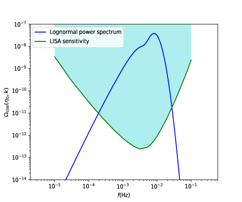
Figure 4.1: The energy density parameter $\Omega_{\mathrm{GW}}(\eta_{0},k)$ for a lognormal curvature power spectrum [see Eq. (4.33)] superimposed to the gravitational wave sensitivity curve of LISA  [256].

4.3 Induced gravitational waves produced in a PBH-dominated era (research article)

Having presented before the basics of the calculation of second order induced gravitational waves from first order scalar perturbations in the case of GW production in a radiation-dominated era, we recap here the main results of our work [32] in which gravitational waves are produced in an era of domination of ultralight PBHs with masses $m_{\mathrm{PBH}}<10^{9}\mathrm{g}$ by emphasizing the differences with the case of induced GWs produced in a RD universe.

Firstly, we should stress out that contrary to the induced GWs produced in a RD era where the gauge-dependence of GWs mentioned in Sec. 4.2.1 is expected to disappear in the late-time limit due to diffusion damping  [242, 243, 244, 245] this does not happen for GWs produced in a matter-dominated era, like the one driven by PBHs. However, in   [32] we do not derive observable predictions, but we rather investigate a GW backreaction problem, which we assume bears little dependence on the gauge. In particular, if the energy density carried by gravitational waves overcomes the one of the background, one expects perturbation theory to break down in any gauge.

In addition, we should underline the nature of the induced GWs studied in [32] as well. In the majority of the literature, induced GWs are sourced be primordial scalar perturbations which have preceded and given rise to PBHs. However, in our work [32] the induced GWs are sourced by scalar perturbations underlain by PBHs themselves. For this reason, by considering monochromatic PBHs produced in a RD universe with their initial spatial distribution being of Poisson type (unclustered), we treated the PBH energy density perturbations as isocurvature perturbations and we extracted at the end the power spectrum of the gravitational potential $\mathcal{P}_{\Phi}(k)$ underlain by a gas of PBHs during the subsequent PBH domination era. Finally, by plugging our expression for $\mathcal{P}_{\Phi}(k)$ in Eq. (4.23) and making use of Eq. (4.25) we computed the GW spectrum $\Omega_{\mathrm{GW}}(\eta,k)$.

Another aspect which should be emphasized here is that in our work  [32], we considered GWs produced during a PBH-dominated era, where $\Phi=\mathrm{constant}$, a fact which forces the source term (4.6) to be constant and as a consequence the equation of motion (4.5) for the tensor modes is not anymore a free-wave equation. The amplitude of gravitational waves converges then to a solution constant in time, which highly suppresses the kinetic contribution compared to the gradient contribution in Eq. (4.15). Consequently, in the case of induced GWs produced during a PBH-dominated era the result (4.25) should be divided by two.

Finally, by making use of Eq. (4.25), we extracted both numerically and analytically $\Omega_{\mathrm{GW}}(\eta_{\mathrm{evap}},k)$ at evaporation time $\eta_{\mathrm{evap}}$ and we found that it crucially depends on two parameters, namely the PBH mass, $m_{\mathrm{PBH}}$ and the initial abundance of PBHs at formation time $\Omega_{\mathrm{PBH,f}}$. Typically, we found that the amount of gravitational waves increases with $m_{\mathrm{PBH}}$, since heavier black holes live longer, hence dominate the universe for a longer period before they evaporate, and with $\Omega_{\mathrm{PBH,f}}$, since more abundant black holes dominate the universe earlier, hence for a longer period too.

Subsequently, by integrating $\Omega_{\mathrm{GW}}(\eta_{\mathrm{evap}},k)$ over the relevant modes $k$ we required that the induced GWs produced during the PBH-dominated era are not overproduced, i.e. $\Omega_{\mathrm{GW,tot}}(\eta_{\mathrm{evap}})<1$, deriving in this way both analytically and numerically the following upper bound constraint on the initial abundance of PBHs, $\Omega_{\mathrm{PBH,f}}$, as a function of their mass $m_{\mathrm{PBH}}$:

$$\Omega_{\mathrm{PBH,f}}<1.4\times 10^{-4}\left(\frac{10^{9}\mathrm{g}}{m_{\mathrm{PBH}}}\right)^{1/4}.$$ (4.34)

At this point, let us stress out that since PBHs with masses smaller than $10^{9}\mathrm{g}$ evaporate before BBN, they cannot be directly constrained (at least without making further assumption, see e.g. [257]). Therefore, to the best of our knowledge, the above constraint is the first one ever derived on ultra-light PBHs. We should also underline that given the fact that we have not assumed a specific PBH production mechanism - we just only assumed that initially PBHs are unclustered and they all have the same mass - the constraint quoted in Eq. (4.34) is rather model independent. For more details see our relevant research article attached below. See pages 2 of Papers/Papanikolaou_2021_J_Cosmol_Astropart_Phys_2021_053.pdf

Chapter 5 PBH formation for an anisotropic perfect fluid

Up to now, most of the research works in the literature model the PBH gravitational collapse as spherical and isotropic due to its calculational simplicity . In particular, in the context of peak theory, within which PBHs are often studied, rare large peaks which collapse to form PBHs are expected to be quasi spherical  [104]. However, one should go beyond these assumptions to model realistically the PBH gravitational collapse process. Regarding the spherical symmetry hypothesis, there were some early studies going beyond and adopting the “pancake” collapse  [260, 261, 262, 263] as well as some recent ones focusing on a non-spherical collapse of PBHs in a matter domination universe  [264] and on the ellipsoidal collapse of PBHs  [124].

Regarding the anisotropic nature of the gravitational collapse, to the best of our knowledge there is no systematic treatment of this topic in the context of PBHs. In general, one expects to have anisotropies in theories with scalar fields and multifluids where the anisotropy is described in spherical symmetry as a difference between the radial and the tangential pressure  [259]. In addition, in the astrophysics context, there has been done a huge progress in the study of anisotropic star solutions in GR which can be obtained both analytically [265, 266, 267, 268, 269, 270, 271] and numerically  [272, 273] but which do not treat the anisotropic character of the collapse in a covariant way. In a recent study  [274] a covariant formulation has been proposed to study anisotropic stars as ultracompact objects mimicking the dynamical behavior of a black-hole .

Inspired by this work, we study here the anisotropic formulation of the initial conditions for the collapse of cosmological perturbations into PBHs, giving at the end some results for the possible effect of the anisotropy on the PBH formation threshold, $\delta_{\mathrm{c}}$. Initially, we review the Misner-Sharp and Misner-Hernadez hydrodynamic equations used to describe the dynamical evolution of a spherically symmetric configuration. Then, we discuss a covariant form for the equation of state of an anisotropic radiation fluid describing the evolution of cosmological perturbations in the early universe. Afterwards, by making a gradient expansion approximation on superhorizon scales we extract the initial conditions for the hydrodynamic and metric perturbations as well as their dependence on the degree of the anisotropy of the gravitational collapse. Finally, we give a synthetic overview regarding the numerical calculation of the PBH formation threshold, $\delta_{\mathrm{c}}$, and adopting a perturbative approach based on the assumption that $\delta_{\mathrm{c}}$ depends on the shape of the initial energy density profile in the same way as in the isotropic case, we give an estimation regarding the dependence of $\delta_{\mathrm{c}}$ on the degree of anisotropy of the gravitational collapse.

The results and conclusions of this chapter regarding PBH formation for an anisotropic perfect fluid were sumbitted on arXiv  [275] on October 12th after the submission of the manuscript.

5.1 The Misner-Sharp Equations for an anisotropic perfect fluid

Working in spherical symmetry, the space-time metric can be written in the Misner-Sharp form  [130]

$$\mathrm{d}s^{2}=-A^{2}(t,r)\mathrm{d}t^{2}+B^{2}(t,r)\mathrm{d}r^{2}+R^{2}(t,r)\mathrm{d}\Omega^{2}$$ (5.1)

where $R$ is the areal radius, $A$ the lapse function, $B$ a function related to the spatial curvature of the space time, $r$ the radial comoving coordinate, $t$ the cosmic time coordinate and $\mathrm{d}\Omega^{2}$ the solid line infinitesimal element of a unit $2$-sphere, i.e. $\mathrm{d}\Omega^{2}=\mathrm{d}\theta^{2}+\sin^{2}\theta\mathrm{d}\phi^{2}$. This is the so called cosmic time slicing, corresponding to a FLRW metric when the Universe is homogeneous and isotropic. Introducing then the differential operators $D_{t}$ and $D_{t}$

$$D_{t}\equiv\left.\frac{1}{A}\frac{\partial}{\partial t}\right|_{r}\mathrm{\quad and\;\;\;\;}D_{r}\equiv\left.\frac{1}{B}\frac{\partial}{\partial r}\right|_{t},$$ (5.2)

which are basically the derivatives with respect to the proper time and proper space respectively, one can define two auxiliary quantities $U$ and $\Gamma$

$$U\equiv D_{t}R\mathrm{\;\;\;\;and\;\;\;\;}\Gamma\equiv D_{r}R,$$ (5.3)

where $U$ is the radial component of the four-velocity in an “Eulerian” (non comoving) frame and $\Gamma$ is the so called generalized Lorentz factor. In the background homogeneous and isotropic FLRW Universe, $R(t,r)=a(t)r$, $U=H(t)R(t,r)$ and $\Gamma^{2}=1-Kr^{2}$, where $a$ is the scale factor, $H$ is the Hubble parameter and $K$ is the spatial curvature present of the FLRW metric (1.7).

The quantities $U$ and $\Gamma$ are related through the Misner-Sharp mass $M$ which for spherical symmetric spacetimes is defined as  [130, 131]

$$M(t,r)\equiv\frac{R(t,r)}{2}\left[1-\nabla_{\mathrm{\mu}}R(t,r)\nabla^{\mathrm{\mu}}R(t,r)\right],$$ (5.4)

From the above definition one can get the constraint equation

$$\Gamma^{2}=1+U^{2}-\frac{2M}{R}$$ (5.5)

obtained by integrating the 00-component of the Einstein equations.

Regarding the form of the stress-energy tensor for an anisotropic perfect fluid, it can be written in a covariant way  [274] as

$$T_{\mathrm{\mu\nu}}=\rho u_{\mathrm{\mu}}u_{\mathrm{\nu}}+p_{\mathrm{r}}k_{\mathrm{\mu}}k_{\mathrm{\nu}}+p_{\mathrm{t}}\Pi_{\mathrm{\mu\nu}},$$ (5.6)

where $p_{r}$ and $p_{t}$ are the radial and tangential pressure respectively, $u_{\mathrm{\mu}}$ is the fluid four-velocity and $k_{\mathrm{\mu}}$ is a unit spacelike vector orthogonal to $u_{\mathrm{\mu}}$, i.e $u_{\mathrm{\mu}}u^{\mathrm{\mu}}=-1=-k_{\mathrm{\mu}}k^{\mathrm{\mu}}$ and $u^{\mathrm{\mu}}k_{\mathrm{\mu}}=0$. $\Pi_{\mathrm{\mu\nu}}=g_{\mathrm{\mu\nu}}+u_{\mathrm{\mu}}u_{\mathrm{\nu}}-k_{\mathrm{\mu}}k_{\mathrm{\nu}}$ is a projection onto a two surface orthogonal to $u^{\mathrm{\mu}}$ and $k^{\mathrm{\mu}}$. Working now in the comoving frame of the fluid we get that $u_{\mathrm{\mu}}=(-A,0,0,0)$ and $k_{\mathrm{\mu}}=(0,B,0,0)$. For an anisotropic spherically symmetric fluid, one has $p_{\mathrm{r}}\neq p_{\mathrm{t}}$.

Considering now the Einstein field equations $G^{\mathrm{\mu}}_{\mathrm{\nu}}=8\pi T^{\mathrm{\mu}}_{\mathrm{\nu}}$ and the conservation of the stress energy tensor $\nabla_{\mathrm{\mu}}T^{\mathrm{\mu\nu}}=0$, one can obtain the Misner-Sharp hydrodynamic set equations [130, 276] for an anisotropic spherically symmetric fluid with $p_{\mathrm{r}}\neq p_{\mathrm{t}}$:

$$D_{t}U=-\frac{\Gamma}{\rho+p_{\mathrm{r}}}\left[D_{r}p_{\mathrm{r}}+\frac{2\Gamma}{R}\left(p_{\mathrm{r}}-p_{\mathrm{t}}\right)\right]-\frac{M}{R^{2}}-4\pi Rp_{\mathrm{r}}$$ (5.7)

$$\frac{D_{t}\rho_{0}}{\rho_{0}}=-\frac{1}{R^{2}\Gamma}D_{r}\left(R^{2}U\right)$$

$$\frac{D_{t}\rho}{\rho+p_{\mathrm{r}}}=\frac{D_{t}\rho_{0}}{\rho_{0}}+\frac{2U}{R}\frac{p_{\mathrm{r}}-p_{\mathrm{t}}}{\rho+p_{\mathrm{r}}}$$

$$\frac{D_{r}A}{A}=-\frac{1}{\rho+p_{\mathrm{r}}}\left[D_{r}p_{\mathrm{r}}+\frac{2\Gamma}{R}\left(p_{\mathrm{r}}-p_{\mathrm{t}}\right)\right]$$

$$D_{r}M=4\pi R^{2}\Gamma\rho$$

$$D_{t}M=-4\pi R^{2}Up_{\mathrm{r}}$$

$$D_{t}\Gamma=-\frac{U}{\rho+p_{\mathrm{r}}}\left[D_{r}p_{\mathrm{r}}+\frac{2\Gamma}{R}\left(p_{\mathrm{r}}-p_{\mathrm{t}}\right)\right],$$

where one can appreciate the additional terms appearing when $p_{\mathrm{r}}\neq p_{\mathrm{t}}$. This system of differential equations, combined with the constraint equation given by Eq. (5.5), can be solved once the equations of state for $p_{\mathrm{r}}$ and $p_{\mathrm{t}}$ are specified. In the context of PBH formation with a massless radiation fluid, one of these equations of state can be obtained assuming, as it looks reasonable, the conservation of the trace, i.e. $T^{\mathrm{\mu}}_{\mathrm{\mu}}=0$  [277], which gives an additional constraint relation between $p_{\mathrm{r}}$ and $p_{\mathrm{t}}$,

$$\rho-p_{\mathrm{r}}-2p_{\mathrm{t}}=0.$$ (5.8)

5.2 The Misner-Hernadez Equations for an anisotropic perfect fluid

When using the Misner-Sharp equations presented in the previous section to study the gravitational collapse process leading to the formation of a black hole, one is facing a well known problem associated to the cosmic time slicing. Because the observer is comoving with the fluid, it is possible to follow the evolution of the region both inside and outside the apparent horizon up to the formation of the singularity. However, in this slicing this is reached when the matter outside the horizon is still collapsing into the black hole. Therefore without doing something, the formation of the singularity is going to prevent following the rest of the outer evolution, computing also the final mass of the black hole, which is one of the fundamental outcomes of such simulations. For this reason, despite the simplicity and intuitiveness of the cosmic time slicing one should consider a null foliation of spacetime, characterized by a far distant observer, in order to track consistently the gravitational collapse process . To do so, we revise here the Misner-Hernadez formulation of the Einstein’s equations in which the time variable is now the “observer time” defined as the time at which an outgoing radial null ray emitted from an event reaches a distant observer. In this way, the formation of the singularity is screened by the asymptotic formation of the apparent horizon because of the infinite redshift associated to signals emitted from the region where the apparent horizon forms  [278], and all the evolution of the region outside the apparent horizon can be followed.

An outgoing null ray is described by the equation

$$A\mathrm{d}t=B\mathrm{d}r$$ (5.9)

and the observer time $u$ is defined by

$$G(r,u)\mathrm{d}u=A(r,t)\mathrm{d}t-B(r,t)\mathrm{d}r,$$ (5.10)

which inserted into the metric 5.1 allows to obtain the following form:

$$\mathrm{d}s^{2}=-G^{2}\mathrm{d}u^{2}-2GB\mathrm{d}u\mathrm{d}r+R^{2}\mathrm{d}\Omega^{2},$$ (5.11)

where the function $G(r,u)$ plays the role of the lapse in the null slicing and satisfies the following useful relation [See Appendix A.2]:

$$\frac{D_{k}G}{G}=\frac{D_{r}A}{A}+\frac{D_{t}B}{B}=\frac{D_{r}A}{A}+\frac{D_{r}U}{\Gamma}.$$ (5.12)

The operators defined in Eq. (5.2) are given by

$$D_{k}\equiv\left.\frac{1}{B}\frac{\partial}{\partial r}\right|_{u}=D_{r}+D_{t},\quad D_{t}\equiv\left.\frac{1}{G}\frac{\partial}{\partial u}\right|_{r},$$ (5.13)

$\Gamma=D_{r}R=D_{k}R-U$ and the equations seen in Eq. (5.7) take the following form, derived for the first time, in the isotropic limit, by Misner-Hernandez:

$$D_{t}U=-\frac{\Gamma}{\rho+p_{\mathrm{r}}}\left[D_{k}p_{\mathrm{r}}-D_{t}p_{\mathrm{r}}+\frac{2\Gamma}{R}(p_{\mathrm{r}}-p_{\mathrm{t}})\right]-\frac{M}{R^{2}}-4\pi Rp_{\mathrm{r}}$$ (5.14)

$$\frac{D_{t}\rho_{0}}{\rho_{0}}=\frac{1}{\Gamma}\left(D_{k}U-D_{t}U\right)-\frac{2U}{R}$$

$$\frac{D_{t}\rho}{\rho+p_{\mathrm{r}}}=\frac{D_{t}\rho_{0}}{\rho_{0}}+\frac{2U}{R}\frac{p_{\mathrm{r}}-p_{\mathrm{t}}}{\rho+p_{\mathrm{r}}}$$

$$\frac{D_{k}G}{G}=\frac{1}{\Gamma}\left[D_{k}U+\frac{M}{R^{2}}+4\pi Rp_{\mathrm{r}}\right]\Leftrightarrow D_{k}\left(\frac{\Gamma+U}{G}\right)=-\frac{4\pi R}{G}(\rho+p_{\mathrm{r}})$$

$$D_{k}M=4\pi R^{2}(\Gamma\rho-p_{\mathrm{r}}U)$$

$$D_{t}M=-4\pi R^{2}Up_{\mathrm{r}}$$

$$D_{t}\Gamma=-\frac{U}{\rho+p_{\mathrm{r}}}\left[D_{k}p_{\mathrm{r}}-D_{t}p_{\mathrm{r}}+\frac{2\Gamma}{R}(p_{\mathrm{r}}-p_{\mathrm{t}})\right].$$

At the computational level, the strategy adopted is the following: first, we perturb the Misner-Sharp equations by performing the gradient expansion approximation on the superhorizon regime in order to specify the initial conditions on a space-like slice at constant cosmic time in terms of a time-independent curvature profile. We do so because in such slicing we know how to specify a consistent set of cosmological perturbations. These initial conditions are then evolved with the Misner-Sharp equations (5.7) in order to generate a second set of initial data on a null slice at constant observer time (outgoing null ray). Finally, this second set of the initial data can then be evolved with the Misner-Hernadez equations (5.14), following the full evolution of the perturbations until an apparent horizon is formed in case of a perturbation with an amplitude larger than the threshold, or seeing that the perturbation bounces and disperses if the amplitude is below the threshold. For more details regarding the numerical scheme see  [279, 132].

5.3 The equation of state of an anisotropic fluid

After having derived the Einstein equations for an anisotropic fluid in the cosmic and null time slicing, we introduce here a covariant formulation modeling the difference between the radial and tangential pressures of the collapsing fluid in terms of pressure or energy density gradients. In particular, following [274, 280] the difference $p_{\mathrm{t}}-p_{\mathrm{r}}$ can be expressed, to a certain degree of arbitrariness, in a covariant form as

$$p_{\mathrm{t}} = p_{\mathrm{r}}+\lambda f(r,t)k^{\mu}\nabla_{\mu}p_{\mathrm{r}}\quad\textrm{(pressure gradients)}$$

or

$$p_{\mathrm{t}} = p_{\mathrm{r}}+\lambda f(r,t)k^{\mu}\nabla_{\mu}\rho\quad\ \textrm{(energy density gradients)},$$ (5.16)

where $f(r,t)$ is a generic function of $r$ and $t$ while $\lambda$ is a parameter tuning the level of the anisotropy of the collapse. Using the metric (5.1) one can show that $k^{\mu}\nabla_{\mu}=D_{r}$. At this point, one should mention that the Minser-Sharp equations (5.7) should be regularized in the following way at $R=0$  [280]:

$$\lim_{R\rightarrow 0}\frac{p_{\mathrm{r}}-p_{\mathrm{t}}}{R}=0.$$ (5.17)

A possible choice for $f(r,t)$ satisfying the boundary condition (5.17) and keeping the parameter $\lambda$ dimensionless, without introducing an additional characteristic scale into the problem, is $f(r,t)=R(r,t)$. In this case, using Eq. (5.3) and Eq. (5.16) combined with Eq. (5.8), the equations of state for $p_{\mathrm{r}}$ and $p_{\mathrm{t}}$ read as

$$p_{\mathrm{r}} = \frac{1}{3}\left[\rho-2\lambda RD_{r}p_{\mathrm{r}}\right],\quad p_{\mathrm{t}}=\frac{1}{3}\left[\rho+\lambda RD_{r}p_{\mathrm{r}}\right]\quad\textrm{(pressure gradients)}$$ (5.18)

$$p_{\mathrm{r}} = \frac{1}{3}\left[\rho-2\lambda RD_{r}\rho\right],\quad p_{\mathrm{t}}=\frac{1}{3}\left[\rho+\lambda RD_{r}\rho\right]\quad\textrm{(energy density gradients).}$$ (5.19)

Another interesting possibility is to choose $f(r,t)=\rho^{n}(r,t)$, where $n$ is an integer. In this last case, the anisotropy parameter $\lambda$ is in general dimensionful but the equations of state for $p_{\mathrm{r}}$ and $p_{\mathrm{t}}$ depend only on thermodynamic quantities, namely on $p_{\mathrm{r}}$ and $\rho$, which are all local quantities of the comoving fluid element, a key difference with respect to the previous model. Using this choice, one obtains that

$$p_{\mathrm{r}} = \frac{1}{3}\left[\rho-2\lambda\rho^{n}D_{r}p_{\mathrm{r}}\right],\quad p_{\mathrm{t}}=\frac{1}{3}\left[\rho+\lambda\rho^{n}D_{r}p_{\mathrm{r}}\right]\quad\textrm{(pressure gradients)}$$ (5.20)

$$p_{\mathrm{r}} = \frac{1}{3}\left[\rho-2\lambda\rho^{n}D_{r}\rho\right],\quad p_{\mathrm{t}}=\frac{1}{3}\left[\rho+\lambda\rho^{n}D_{r}\rho\right]\quad\textrm{(energy dens. gradients).}$$ (5.21)

As one can see, from Eq. (5.18) and Eq. (5.20), in the limit $\lambda=0$ one reproduces the isotropic limit in which $p_{\mathrm{r}}=p_{\mathrm{t}}=\rho/3$. Below, we give the form of the Misner-Sharp equations (5.7) in the anisotropic regime where $p_{\mathrm{r}}\neq p_{\mathrm{t}}$ for $f(r,t)=R(r,t)$ and $f(r,t)=\rho^{n}(r,t)$.

• $f(r,t)=R(r,t),p_{\mathrm{r}}-p_{\mathrm{t}}=-\lambda RD_{r}p_{\mathrm{r}}$

  $$D_{t}U=-\frac{\Gamma(1-2\lambda\Gamma)}{\rho+p_{\mathrm{r}}}D_{r}p_{\mathrm{r}}-\frac{M}{R^{2}}-4\pi Rp_{\mathrm{r}}$$ (5.22)

  $$\frac{D_{t}\rho}{\rho+p_{\mathrm{r}}}=\frac{D_{t}\rho_{0}}{\rho_{0}}-2\lambda U\frac{D_{r}p_{\mathrm{r}}}{\rho+p_{\mathrm{r}}}$$

  $$\frac{D_{r}A}{A}=-\frac{(1-2\lambda\Gamma)}{\rho+p_{\mathrm{r}}}D_{r}p_{\mathrm{r}}$$

  $$D_{t}\Gamma=-\frac{U(1-2\lambda\Gamma)}{\rho+p_{\mathrm{r}}}D_{r}p_{\mathrm{r}}$$

• $f(r,t)=R(r,t),p_{\mathrm{r}}-p_{\mathrm{t}}=-\lambda RD_{r}\rho$

  $$D_{t}U=-\frac{\Gamma}{\rho+p_{\mathrm{r}}}(D_{r}p_{\mathrm{r}}-2\lambda\Gamma D_{r}\rho)-\frac{M}{R^{2}}-4\pi Rp_{\mathrm{r}}$$ (5.23)

  $$\frac{D_{t}\rho}{\rho+p_{\mathrm{r}}}=\frac{D_{t}\rho_{0}}{\rho_{0}}-2\lambda U\frac{D_{r}\rho}{\rho+p_{\mathrm{r}}}$$

  $$\frac{D_{r}A}{A}=-\frac{1}{\rho+p_{\mathrm{r}}}(D_{r}p_{\mathrm{r}}-2\lambda\Gamma D_{r}\rho)$$

  $$D_{t}\Gamma=-\frac{U}{\rho+p_{\mathrm{r}}}(D_{r}p_{\mathrm{r}}-2\lambda\Gamma D_{r}\rho)$$

• $f(r,t)=\rho^{n}(r,t),p_{\mathrm{r}}-p_{\mathrm{t}}=-\lambda\rho^{n}(r,t)D_{r}p_{\mathrm{r}}$

  $$D_{t}U=-\frac{\Gamma}{\rho+p_{\mathrm{r}}}\left(1-\frac{2\lambda\Gamma\rho^{n}}{R}\right)D_{r}p_{\mathrm{r}}-\frac{M}{R^{2}}-4\pi Rp_{\mathrm{r}}$$ (5.24)

  $$\frac{D_{t}\rho}{\rho+p_{\mathrm{r}}}=\frac{D_{t}\rho_{0}}{\rho_{0}}-\frac{2\lambda U\rho^{n}}{R}\frac{D_{r}p_{\mathrm{r}}}{\rho+p_{\mathrm{r}}}$$

  $$\frac{D_{r}A}{A}=-\frac{D_{r}p_{\mathrm{r}}}{\rho+p_{\mathrm{r}}}\left(1-\frac{2\lambda\Gamma\rho^{n}}{R}\right)$$

  $$D_{t}\Gamma=-\frac{U}{\rho+p_{\mathrm{r}}}\left(1-\frac{2\lambda\Gamma\rho^{n}}{R}\right)D_{r}p_{\mathrm{r}}$$

• $f(r,t)=\rho^{n}(r,t),p_{\mathrm{r}}-p_{\mathrm{t}}=-\lambda\rho^{n}(r,t)D_{r}\rho$

  $$D_{t}U=-\frac{\Gamma}{\rho+p_{\mathrm{r}}}\left(D_{r}p_{\mathrm{r}}-\frac{2\lambda\Gamma\rho^{n}}{R}D_{r}\rho\right)-\frac{M}{R^{2}}-4\pi Rp_{\mathrm{r}}$$ (5.25)

  $$\frac{D_{t}\rho}{\rho+p_{\mathrm{r}}}=\frac{D_{t}\rho_{0}}{\rho_{0}}-\frac{2\lambda U\rho^{n}}{R}\frac{D_{r}\rho}{\rho+p_{\mathrm{r}}}$$

  $$\frac{D_{r}A}{A}=-\frac{1}{\rho+p_{\mathrm{r}}}\left(D_{r}p_{\mathrm{r}}-\frac{2\lambda\Gamma\rho^{n}}{R}D_{r}\rho\right)$$

  $$D_{t}\Gamma=-\frac{U}{\rho+p_{\mathrm{r}}}\left(D_{r}p_{\mathrm{r}}-\frac{2\lambda\Gamma\rho^{n}}{R}D_{r}\rho\right)$$

5.4 The quasi homogeneous solution

Having introduced a covariant formulation of the equation of state for a spherically symmetric anisotropic fluid, one should specify the initial conditions for all the relevant quantities describing a cosmological perturbation on superhorizon scales. To do so, let us consider the asymptotic solution of the Einstein’s equations in the limit of $t\rightarrow 0$. This corresponds to a FLRW metric with an $r$ dependent curvature profile $K(r)$ which does not depend on time,

$$\mathrm{d}s^{2}_{\mathrm{AQH}}=-\mathrm{d}t^{2}+a^{2}(t)\left[\frac{\mathrm{d}r^{2}}{1-K(r)r^{2}}+r^{2}\mathrm{d}\Omega^{2}\right].$$ (5.26)

The above solution is often quoted as the Asymptotic Quasi Homogeneous solution (AQH) (as $t\rightarrow 0$) [281] and within this formulation of the metric, $K(r)$ can be seen as an initial curvature profile specified on superhorizon scales . At this point, it is important to stress out that $K(r)$ corresponds to arbitrarily large metric perturbations while the hydrodynamic perturbations, i.e. energy density and velocity ones, vanish asymptotically as $t\rightarrow 0$ and therefore on such regime they can be treated as small perturbations. One can then solve analytically the hydrodynamic equations and write self-consistently the initial conditions for the energy density, the velocity perturbations and all the relevant variables of the equations as a function of the curvature profile $K(r)$ at a time when the quasi-homogeneous solution is valid at certain order.

Considering perturbations well outside the horizon, all the hydrodynamic and metric quantities are nearly homogeneous and their perturbations are small deviations away from their background value. To parametrise these deviations, we introduce a fictitious parameter $\epsilon$ defined as the ratio between the Hubble radius $H^{-1}$ and the characteristic physical scale, $L$, of the collapsing region,

$$\epsilon(t)=\frac{H^{-1}}{L}=\frac{1}{H(t)a(t)r_{\mathrm{m}}}\ll 1,$$ (5.27)

where $r_{\mathrm{m}}$ is the comoving characteristic scale of the collapsing region. In this way, all quantities can be written as a power series in $\epsilon$. Thus, considering only the growing mode which is of $O(\epsilon^{2})$ in the first non zero term of the expansion  [282, 89], at first order one has for the hydrodynamic variables $\rho$, $U$, $p_{\mathrm{r}}$, $p_{\mathrm{t}}$ and $M$ that [133]

$$\begin{split}\rho&=\rho_{\mathrm{b}}(t)\left[1+\epsilon^{2}\tilde{\rho}(r,t)\right]\\ p_{\mathrm{r}}&=\frac{\rho_{\mathrm{b}}(t)}{3}\left[1+\epsilon^{2}\tilde{p}_{\mathrm{r}}(r,t)\right]\\ p_{\mathrm{t}}&=\frac{\rho_{\mathrm{b}}(t)}{3}\left[1+\epsilon^{2}\tilde{p}_{\mathrm{t}}(r,t)\right]\\ U&=H(t)R\left[1+\epsilon^{2}\tilde{U}(r,t)\right]\\ M&=\frac{4\pi}{3}\rho_{\mathrm{b}}(t)R^{3}\left[1+\epsilon^{2}\tilde{M}(r,t)\right].\end{split}$$ (5.28)

This approach is known in the literature as the long wavelength approach  [90], or gradient expansion [283], or separate universe hypothesis  [284, 282] and reproduces the time evolution of the linear perturbation theory.

Regarding the metric components $A$, $B$ and $R$, which are coupled to the matter ones through Einstein’s equations, one can write in the same way that

$$\begin{split}A&=1+\epsilon^{2}\tilde{A}(r,t)\\ B&=\frac{R^{\prime}}{\mathchoice{{\hbox{$\displaystyle\sqrt{1-K(r)r^{2}\,}$}\lower 0.4pt\hbox{\vrule height=7.5pt,depth=-6.00003pt}}}{{\hbox{$\textstyle\sqrt{1-K(r)r^{2}\,}$}\lower 0.4pt\hbox{\vrule height=7.5pt,depth=-6.00003pt}}}{{\hbox{$\scriptstyle\sqrt{1-K(r)r^{2}\,}$}\lower 0.4pt\hbox{\vrule height=5.25pt,depth=-4.20003pt}}}{{\hbox{$\scriptscriptstyle\sqrt{1-K(r)r^{2}\,}$}\lower 0.4pt\hbox{\vrule height=3.75pt,depth=-3.00002pt}}}}\left[1+\epsilon^{2}\tilde{B}(r,t)\right]\\ R&=a(t)r\left[1+\epsilon^{2}\tilde{R}(r,t)\right].\end{split}$$ (5.29)

The next step is to perform now the perturbative analysis and extract the initial conditions for the hydrodynamic and metric perturbations as a function of the curvature profile $K(r)$. To do so, by performing the gradient expansion at the level of the Misner-Sharp equations (5.7), we extract below the equations for the metric and the hydrodynamic perturbations without specifying a specific model describing the difference $p_{\mathrm{r}}-p_{\mathrm{t}}$.

We start initially with the metric perturbations $\tilde{A}$, $\tilde{B}$ and $\tilde{R}$. From the definition of $U$ one has that $\dot{R}=AU$. Perturbing this equation by keeping only first order terms, i.e. $\sim O(\epsilon^{2})$, one gets for $\tilde{R}$ that it should obey the following equation:

$$\begin{split}\dot{a}(1+\epsilon^{2}\tilde{R})+a\left(\epsilon^{2}\tilde{R}\right)^{.}&=(1+\epsilon^{2}\tilde{A})HR(1+\epsilon^{2}\tilde{U})\Leftrightarrow\\ 2\epsilon\dot{\epsilon}\tilde{R}+\epsilon\dot{\tilde{R}}&=\epsilon H(\tilde{A}+\tilde{U})\Leftrightarrow\\ 2\tilde{R}+\frac{\partial\tilde{R}}{\partial N}&=\tilde{A}+\tilde{U},\end{split}$$ (5.30)

where $N=\ln(a/a_{\mathrm{ini}})$ is the number of e-folds and $a_{\mathrm{ini}}$ is the scale factor at an initial time. In the last step, we used the fact that $\dot{\epsilon}/\epsilon=H$. Then, from the $01$ Einstein equation one can easily get that $\frac{\dot{B}}{B}=A\frac{U^{\prime}}{R^{\prime}}$. Combining the above equation with $\dot{R}=AU$ we obtain that $\frac{\dot{B}}{B}-\frac{\dot{R}^{\prime}}{R^{\prime}}=-\frac{A^{\prime}U}{R^{\prime}}$, which, once perturbed by keeping orders up to $O(\epsilon^{2})$, gives the following equation for $\tilde{B}$:

$$2\tilde{B}+\frac{\partial\tilde{B}}{\partial N}=-r\tilde{A}^{\prime}.$$ (5.31)

The prime ^′ denotes differentiation with respect to the radial comoving coordinate. Finally, regarding the perturbation of the lapse function $\tilde{A}$, perturbing the equation $\frac{D_{r}A}{A}=-\frac{1}{\rho+p_{\mathrm{r}}}\left[D_{r}p_{\mathrm{r}}+\frac{2\Gamma}{R}\left(p_{\mathrm{r}}-p_{\mathrm{t}}\right)\right]$ one obtains that

$$\tilde{A}^{\prime}=-\frac{1}{4}\left[\tilde{p}^{\prime}_{\mathrm{r}}+\frac{2}{r}\left(\tilde{p}_{\mathrm{r}}-\tilde{p}_{\mathrm{t}}\right)\right].$$ (5.32)

We continue the perturbative gradient expansion scheme considering the hydrodynamic perturbations $\tilde{U}$, $\tilde{\rho}$ and $\tilde{M}$. Regarding $\tilde{\rho}$ one perturbs the equation $D_{r}M=4\pi R^{2}\Gamma\rho$ which gives

$$\frac{1}{3}(1+\epsilon^{2}\tilde{M})\left[3\frac{R^{\prime}}{R}+\epsilon^{2}\tilde{M}^{\prime}\right]=(1+\epsilon^{2}\tilde{\rho})\frac{R^{\prime}}{R}\Leftrightarrow$$ (5.33)

$$\tilde{\rho}=\frac{1}{3r^{2}}\left(r^{3}\tilde{M}\right)^{\prime}.$$ (5.34)

Then, the equation for $\tilde{M}$, obtained by perturbing $D_{t}M=-4\pi R^{2}Up_{\mathrm{r}}$, reads as

$$(1+\epsilon^{2}\tilde{M})\left[\frac{\dot{\rho}_{\mathrm{b}}}{\rho_{\mathrm{b}}}+3\frac{\dot{R}}{R}+\left(\epsilon^{2}\tilde{M}\right)^{.}\right]=-\frac{\dot{R}}{R}(1+\epsilon^{2}\tilde{p}_{\mathrm{r}})\Leftrightarrow$$ (5.35)

$$\tilde{M}+\frac{\partial\tilde{M}}{\partial N}=-4\tilde{U}-4\tilde{A}-\tilde{p}_{\mathrm{r}}.$$ (5.36)

Regarding $\tilde{U}$, by perturbing Eq. (5.5) one gets that

$$\tilde{U}=\frac{1}{2}\left[\tilde{M}-K(r)r_{\mathrm{m}}^{2}\right].$$ (5.37)

To summarize, the differential equations describing the behavior of the metric and hydrodynamic perturbations in the gradient expansion approximation in which $\epsilon\ll 1$ are:

$$2\tilde{R}+\frac{\partial\tilde{R}}{\partial N} =\tilde{A}+\tilde{U}$$ (5.38)

$$2\tilde{B}+\frac{\partial\tilde{B}}{\partial N} =-r\tilde{A}^{\prime}$$

$$\tilde{A}^{\prime} =-\frac{1}{4}\left[\tilde{p}^{\prime}_{\mathrm{r}}+\frac{2}{r}\left(\tilde{p}_{\mathrm{r}}-\tilde{p}_{\mathrm{t}}\right)\right]$$

$$\tilde{\rho} =\frac{1}{3r^{2}}\left(r^{3}\tilde{M}\right)^{\prime}$$

$$\tilde{M}+\frac{\partial\tilde{M}}{\partial N} =-4\tilde{U}-4\tilde{A}-\tilde{p}_{\mathrm{r}}$$

$$\tilde{U} =\frac{1}{2}\left[\tilde{M}-K(r)r_{\mathrm{m}}^{2}\right].$$

As one may see from the above equations, the only place, in which the dependence on the prescription modeling the difference $p_{\mathrm{r}}-p_{\mathrm{t}}$ enters, is at the level of the differential equation for the lapse function perturbation, $\tilde{A}$.

5.5 The initial conditions in presence of anisotropies

We extract below the initial conditions of the hydrodynamic and metric perturbations as a function of the time-independent curvature profile $K(r)$ by specifying our choice for the EoS of an anisotropic radiation dominated medium.

5.5.1 Equation of state in terms of pressure gradients

We choose here the EoS where the difference $p_{\mathrm{r}}-p_{\mathrm{t}}$ is proportional to pressure gradients [See Eq. (5.3)]. Regarding the free function $f(r,t)$ we choose it to be either $f(r,t)=R(r,t)$ (which is a non local quantity) or $f(r,t)=\rho^{n}(r,t)$ (which is a local quantity).

5.5.1.1 $f(r,t)=R(r,t)$

In this case, the anisotropy parameter $\lambda$ is dimensionless and therefore one does not need to introduce a characteristic scale at the level of the equation of state. Using the EoS (5.18), with a straightforward calculation one has that the constraint equation for $\tilde{p}_{\mathrm{r}}$ reads as

$$\tilde{p}_{\mathrm{r}}-\tilde{\rho}=-\frac{2\lambda r}{3}\mathchoice{{\hbox{$\displaystyle\sqrt{1-K(r)r^{2}\,}$}\lower 0.4pt\hbox{\vrule height=7.5pt,depth=-6.00003pt}}}{{\hbox{$\textstyle\sqrt{1-K(r)r^{2}\,}$}\lower 0.4pt\hbox{\vrule height=7.5pt,depth=-6.00003pt}}}{{\hbox{$\scriptstyle\sqrt{1-K(r)r^{2}\,}$}\lower 0.4pt\hbox{\vrule height=5.25pt,depth=-4.20003pt}}}{{\hbox{$\scriptscriptstyle\sqrt{1-K(r)r^{2}\,}$}\lower 0.4pt\hbox{\vrule height=3.75pt,depth=-3.00002pt}}}\tilde{p}^{\prime}_{\mathrm{r}}=-\frac{2\lambda r}{3}F^{\prime}(r),$$ (5.39)

where

$$F(r)\equiv\int_{0}^{r}\mathchoice{{\hbox{$\displaystyle\sqrt{1-K(r^{\prime})r^{\prime 2}\,}$}\lower 0.4pt\hbox{\vrule height=7.5pt,depth=-6.00003pt}}}{{\hbox{$\textstyle\sqrt{1-K(r^{\prime})r^{\prime 2}\,}$}\lower 0.4pt\hbox{\vrule height=7.5pt,depth=-6.00003pt}}}{{\hbox{$\scriptstyle\sqrt{1-K(r^{\prime})r^{\prime 2}\,}$}\lower 0.4pt\hbox{\vrule height=5.25pt,depth=-4.20003pt}}}{{\hbox{$\scriptscriptstyle\sqrt{1-K(r^{\prime})r^{\prime 2}\,}$}\lower 0.4pt\hbox{\vrule height=3.75pt,depth=-3.00002pt}}}\tilde{p}^{\prime}_{\mathrm{r}}(r^{\prime})\mathrm{d}r^{\prime}=-\frac{3}{2\lambda}\int^{r}_{0}\frac{\tilde{p}_{\mathrm{r}}-\tilde{\rho}}{r^{\prime}}\mathrm{d}r^{\prime},$$ (5.40)

and the corresponding equation for the lapse perturbation $\tilde{A}$ reads as

$$\tilde{A}^{\prime}=-\frac{1}{4}\left(\tilde{p}^{\prime}_{\mathrm{r}}-2\lambda\mathchoice{{\hbox{$\displaystyle\sqrt{1-K(r)r^{2}\,}$}\lower 0.4pt\hbox{\vrule height=7.5pt,depth=-6.00003pt}}}{{\hbox{$\textstyle\sqrt{1-K(r)r^{2}\,}$}\lower 0.4pt\hbox{\vrule height=7.5pt,depth=-6.00003pt}}}{{\hbox{$\scriptstyle\sqrt{1-K(r)r^{2}\,}$}\lower 0.4pt\hbox{\vrule height=5.25pt,depth=-4.20003pt}}}{{\hbox{$\scriptscriptstyle\sqrt{1-K(r)r^{2}\,}$}\lower 0.4pt\hbox{\vrule height=3.75pt,depth=-3.00002pt}}}\right).$$ (5.41)

These equations coupled with Eq. (5.38) allows to find the explicit dependence of the initial perturbation profiles on the curvature profile $K(r)$. Let us start with the metric perturbations $\tilde{A}$, $\tilde{R}$ and $\tilde{B}$. Integrating Eq. (5.41) and using the fact that $\tilde{\rho}(0)=\tilde{p}_{\mathrm{r}}(0)$, as it can be seen by Eq. (5.39), one can infer that

$$\tilde{A}-\tilde{A}(0)=-\frac{1}{4}\tilde{p}_{\mathrm{r}}+\frac{\tilde{\rho}(0)}{4}+\frac{\lambda}{2}F(r).$$ (5.42)

At $r=\infty$, where $\tilde{p}_{\mathrm{r}}(\infty)=0$, from the above equation one has that

$$\tilde{A}(\infty)=0=\tilde{A}(0)+\frac{\tilde{\rho}(0)}{4}+\frac{\lambda}{2}F(\infty)\Leftrightarrow\tilde{A}(0)=-\frac{1}{4}\left[\tilde{\rho}(0)+2\lambda F(\infty)\right].$$ (5.43)

Thus, plugging Eq. (5.43) into Eq. (5.42) and taking into account Eq. (5.39), one gets that

$$\tilde{A}=-\frac{\tilde{\rho}}{4}+\frac{\lambda}{2}\left[\frac{r\mathcal{F}^{\prime}(r)}{3}+\mathcal{F}(r)\right],$$ (5.44)

where we have introduced the function $\mathcal{F}(r)$ defined as

$$\mathcal{F}(r)\equiv F(r)-F(\infty)=-\int_{r}^{\infty}\frac{\partial\tilde{p}_{\mathrm{r}}(r^{\prime})}{\partial r^{\prime}}\mathchoice{{\hbox{$\displaystyle\sqrt{1-K(r^{\prime})r^{\prime 2}\,}$}\lower 0.4pt\hbox{\vrule height=7.5pt,depth=-6.00003pt}}}{{\hbox{$\textstyle\sqrt{1-K(r^{\prime})r^{\prime 2}\,}$}\lower 0.4pt\hbox{\vrule height=7.5pt,depth=-6.00003pt}}}{{\hbox{$\scriptstyle\sqrt{1-K(r^{\prime})r^{\prime 2}\,}$}\lower 0.4pt\hbox{\vrule height=5.25pt,depth=-4.20003pt}}}{{\hbox{$\scriptscriptstyle\sqrt{1-K(r^{\prime})r^{\prime 2}\,}$}\lower 0.4pt\hbox{\vrule height=3.75pt,depth=-3.00002pt}}}\mathrm{d}r^{\prime}.$$ (5.45)

Considering now Eq. (5.30) for $\tilde{R}$, one can crearly see that the right-hand side is time-independent because of Eq. (5.44) and Eq. (5.37) allowing $\tilde{R}$ to be written as

$$\tilde{R}=\frac{1}{2}\left(\tilde{A}+\tilde{U}\right)=-\frac{1}{2}\left\{\frac{\tilde{\rho}}{4}-\frac{\lambda}{6}\left[r\mathcal{F}^{\prime}(r)+\mathcal{F}(r)\right]+\frac{1}{6}K(r)r_{\mathrm{m}}^{2}\right\}$$ (5.46)

As for $\tilde{B}$, following the same reasoning, one can see that

$$\tilde{B}=-\frac{r\tilde{A}^{\prime}}{2}=\frac{r}{8}\tilde{p}^{\prime}_{\mathrm{r}}(1-2\lambda\mathchoice{{\hbox{$\displaystyle\sqrt{1-K(r)r^{2}\,}$}\lower 0.4pt\hbox{\vrule height=7.5pt,depth=-6.00003pt}}}{{\hbox{$\textstyle\sqrt{1-K(r)r^{2}\,}$}\lower 0.4pt\hbox{\vrule height=7.5pt,depth=-6.00003pt}}}{{\hbox{$\scriptstyle\sqrt{1-K(r)r^{2}\,}$}\lower 0.4pt\hbox{\vrule height=5.25pt,depth=-4.20003pt}}}{{\hbox{$\scriptscriptstyle\sqrt{1-K(r)r^{2}\,}$}\lower 0.4pt\hbox{\vrule height=3.75pt,depth=-3.00002pt}}})=\frac{r}{8}F^{\prime}(r)\left[\frac{1}{\mathchoice{{\hbox{$\displaystyle\sqrt{1-K(r)r^{2}\,}$}\lower 0.4pt\hbox{\vrule height=7.5pt,depth=-6.00003pt}}}{{\hbox{$\textstyle\sqrt{1-K(r)r^{2}\,}$}\lower 0.4pt\hbox{\vrule height=7.5pt,depth=-6.00003pt}}}{{\hbox{$\scriptstyle\sqrt{1-K(r)r^{2}\,}$}\lower 0.4pt\hbox{\vrule height=5.25pt,depth=-4.20003pt}}}{{\hbox{$\scriptscriptstyle\sqrt{1-K(r)r^{2}\,}$}\lower 0.4pt\hbox{\vrule height=3.75pt,depth=-3.00002pt}}}}-2\lambda\right].$$ (5.47)

To work out the expression for $\tilde{M}$ one can combine Eqs. ((5.36), (5.42) , (5.39) and (5.37) ) and obtain that

$$\tilde{M}+\frac{1}{3}\frac{\partial\tilde{M}}{\partial N}=\frac{2}{3}K(r)r_{\mathrm{m}}^{2}-\frac{2}{3}\lambda\mathcal{F}(r).$$ (5.48)

Following the same reasoning as in the case of $\tilde{R}$, given the time-independent nature of the right-hand side of Eq. (5.48) one can deduce that

$$\tilde{M}=\frac{2}{3}K(r)r_{\mathrm{m}}^{2}-\frac{2}{3}\lambda\mathcal{F}(r).$$ (5.49)

Considering the behavior of $\tilde{U}$, one can plug Eq. (5.49) into Eq. (5.37) to get that

$$\tilde{U}=-\frac{1}{6}K(r)r_{\mathrm{m}}^{2}-\frac{\lambda}{3}\mathcal{F}(r).$$ (5.50)

Finally, by plugging Eq. (5.49) into Eq. (5.34) one obtains the expression for the energy density,

$$\tilde{\rho}=\frac{2}{3}\left\{\frac{\left[r^{3}K(r)\right]^{\prime}}{3r^{2}}r^{2}_{\mathrm{m}}-\lambda\left[\frac{r}{3}\mathcal{F}^{\prime}(r)+\mathcal{F}(r)\right]\right\}.$$ (5.51)

One can further simplify the expressions for $\tilde{A}$, $\tilde{R}$, $\tilde{B}$, $\tilde{M}$, $\tilde{\rho}$ and $\tilde{U}$ writing them in a more compact form. To do so, we introduce the following effective curvature profile,

$$\mathcal{K}(r)\equiv K(r)-\frac{\lambda}{r^{2}_{\mathrm{m}}}\mathcal{F}(r).$$ (5.52)

This allows to write the quasi-homogeneous solution, in a similar form as the isotropic case ($\lambda=0$), introducing the effective energy density and velocity perturbations $\tilde{\rho}_{\mathrm{eff}}$ and $\tilde{U}_{\mathrm{eff}}$ defined as

$$\tilde{\rho}_{\mathrm{eff}}=\tilde{\rho}-2\lambda\left[\frac{r\mathcal{F}^{\prime}(r)}{3}+\mathcal{F}(r)\right],$$ (5.53)

$$\tilde{U}_{\mathrm{eff}}=\tilde{U}+\frac{\lambda}{2}\mathcal{F}(r)=-\frac{1}{6}\mathcal{K}(r)r^{2}_{\mathrm{m}}$$ (5.54)

In this way, the metric and the hydrodynamic perturbations are given by the following expressions:

$$\begin{split}\tilde{A}&=-\frac{\tilde{\rho}}{4}+\frac{\lambda}{2}\left[\frac{r\mathcal{F}^{\prime}(r)}{3}+\mathcal{F}(r)\right]=-\frac{\tilde{\rho}_{\mathrm{eff}}}{4}\\ \tilde{B}&=\frac{r}{8}\mathcal{F}^{\prime}(r)\left[\frac{1}{\mathchoice{{\hbox{$\displaystyle\sqrt{1-K(r)r^{2}\,}$}\lower 0.4pt\hbox{\vrule height=7.5pt,depth=-6.00003pt}}}{{\hbox{$\textstyle\sqrt{1-K(r)r^{2}\,}$}\lower 0.4pt\hbox{\vrule height=7.5pt,depth=-6.00003pt}}}{{\hbox{$\scriptstyle\sqrt{1-K(r)r^{2}\,}$}\lower 0.4pt\hbox{\vrule height=5.25pt,depth=-4.20003pt}}}{{\hbox{$\scriptscriptstyle\sqrt{1-K(r)r^{2}\,}$}\lower 0.4pt\hbox{\vrule height=3.75pt,depth=-3.00002pt}}}}-2\lambda\right]=\frac{r}{8}\tilde{\rho}^{\prime}_{\mathrm{eff}}\\ \tilde{\rho}&=\frac{2}{3}\frac{\left[r^{3}\mathcal{K}(r)\right]^{\prime}}{3r^{2}}r^{2}_{\mathrm{m}}\\ \tilde{U}&=-\frac{1}{6}\mathcal{K}(r)r_{\mathrm{m}}^{2}-\frac{\lambda}{2}\mathcal{F}(r)=\tilde{U}_{\mathrm{eff}}-\frac{\lambda}{2}\mathcal{F}(r)\\ \tilde{M}&=\frac{2}{3}\mathcal{K}(r)r_{\mathrm{m}}^{2}=-4\tilde{U}_{\mathrm{eff}}\\ \tilde{R}&=-\frac{\tilde{\rho}_{\mathrm{eff}}}{8}+\frac{\tilde{U}}{2}.\end{split}$$ (5.55)

To complete this derivation we need to find the function $\mathcal{F}(r)$ defined in Eq. (5.45), which is the integral of the pressure-gradient profile $\frac{\partial\tilde{p}_{\mathrm{r}}}{\partial r}$, corrected by $\Gamma\simeq\mathchoice{{\hbox{$\displaystyle\sqrt{1-K(r)r^{2}\,}$}\lower 0.4pt\hbox{\vrule height=7.5pt,depth=-6.00003pt}}}{{\hbox{$\textstyle\sqrt{1-K(r)r^{2}\,}$}\lower 0.4pt\hbox{\vrule height=7.5pt,depth=-6.00003pt}}}{{\hbox{$\scriptstyle\sqrt{1-K(r)r^{2}\,}$}\lower 0.4pt\hbox{\vrule height=5.25pt,depth=-4.20003pt}}}{{\hbox{$\scriptscriptstyle\sqrt{1-K(r)r^{2}\,}$}\lower 0.4pt\hbox{\vrule height=3.75pt,depth=-3.00002pt}}}$ on super horizon scales, which is measuring the geometrical curvature of the space time. In particular, by combining Eqs. (5.39) and (5.51) one obtains the following integral equation for $\tilde{p}_{\mathrm{r}}$

$$\tilde{p}_{\mathrm{r}}=\frac{2}{3}\left\{\frac{\left[r^{3}K(r)\right]^{\prime}}{3r^{2}}r^{2}_{\mathrm{m}}-\lambda\left[\mathcal{F}(r)+\frac{4}{3}rf(r)\right]\right\}.$$ (5.56)

where

$$f(r)\equiv\frac{\partial\tilde{p}_{\mathrm{r}}}{\partial r}\mathchoice{{\hbox{$\displaystyle\sqrt{1-K(r)r^{2}\,}$}\lower 0.4pt\hbox{\vrule height=7.5pt,depth=-6.00003pt}}}{{\hbox{$\textstyle\sqrt{1-K(r)r^{2}\,}$}\lower 0.4pt\hbox{\vrule height=7.5pt,depth=-6.00003pt}}}{{\hbox{$\scriptstyle\sqrt{1-K(r)r^{2}\,}$}\lower 0.4pt\hbox{\vrule height=5.25pt,depth=-4.20003pt}}}{{\hbox{$\scriptscriptstyle\sqrt{1-K(r)r^{2}\,}$}\lower 0.4pt\hbox{\vrule height=3.75pt,depth=-3.00002pt}}}\,.$$

By differentiating the above equation we can write the following differential equation,

$$\frac{8\lambda}{9}r\mathchoice{{\hbox{$\displaystyle\sqrt{1-K(r)r^{2}\,}$}\lower 0.4pt\hbox{\vrule height=7.5pt,depth=-6.00003pt}}}{{\hbox{$\textstyle\sqrt{1-K(r)r^{2}\,}$}\lower 0.4pt\hbox{\vrule height=7.5pt,depth=-6.00003pt}}}{{\hbox{$\scriptstyle\sqrt{1-K(r)r^{2}\,}$}\lower 0.4pt\hbox{\vrule height=5.25pt,depth=-4.20003pt}}}{{\hbox{$\scriptscriptstyle\sqrt{1-K(r)r^{2}\,}$}\lower 0.4pt\hbox{\vrule height=3.75pt,depth=-3.00002pt}}}f^{\prime}(r) +\left[\frac{14\lambda}{9}\mathchoice{{\hbox{$\displaystyle\sqrt{1-K(r)r^{2}\,}$}\lower 0.4pt\hbox{\vrule height=7.5pt,depth=-6.00003pt}}}{{\hbox{$\textstyle\sqrt{1-K(r)r^{2}\,}$}\lower 0.4pt\hbox{\vrule height=7.5pt,depth=-6.00003pt}}}{{\hbox{$\scriptstyle\sqrt{1-K(r)r^{2}\,}$}\lower 0.4pt\hbox{\vrule height=5.25pt,depth=-4.20003pt}}}{{\hbox{$\scriptscriptstyle\sqrt{1-K(r)r^{2}\,}$}\lower 0.4pt\hbox{\vrule height=3.75pt,depth=-3.00002pt}}}+1\right]f(r)$$ (5.57)

$$-\frac{2}{3}\left\{\frac{\left[r^{3}K(r)\right]^{\prime}}{3r^{2}}\right\}^{\prime}r^{2}_{\mathrm{m}}\mathchoice{{\hbox{$\displaystyle\sqrt{1-K(r)r^{2}\,}$}\lower 0.4pt\hbox{\vrule height=7.5pt,depth=-6.00003pt}}}{{\hbox{$\textstyle\sqrt{1-K(r)r^{2}\,}$}\lower 0.4pt\hbox{\vrule height=7.5pt,depth=-6.00003pt}}}{{\hbox{$\scriptstyle\sqrt{1-K(r)r^{2}\,}$}\lower 0.4pt\hbox{\vrule height=5.25pt,depth=-4.20003pt}}}{{\hbox{$\scriptscriptstyle\sqrt{1-K(r)r^{2}\,}$}\lower 0.4pt\hbox{\vrule height=3.75pt,depth=-3.00002pt}}}=0,$$

with $f(0)=0$ and for $\lambda=0$ we recover the quasi-homogeneous limit,

$$f_{\lambda=0}(r)=\frac{2}{3}\left\{\frac{\left[r^{3}K(r)\right]^{\prime}}{3r^{2}}\right\}^{\prime}r^{2}_{\mathrm{m}}\mathchoice{{\hbox{$\displaystyle\sqrt{1-K(r)r^{2}\,}$}\lower 0.4pt\hbox{\vrule height=7.5pt,depth=-6.00003pt}}}{{\hbox{$\textstyle\sqrt{1-K(r)r^{2}\,}$}\lower 0.4pt\hbox{\vrule height=7.5pt,depth=-6.00003pt}}}{{\hbox{$\scriptstyle\sqrt{1-K(r)r^{2}\,}$}\lower 0.4pt\hbox{\vrule height=5.25pt,depth=-4.20003pt}}}{{\hbox{$\scriptscriptstyle\sqrt{1-K(r)r^{2}\,}$}\lower 0.4pt\hbox{\vrule height=3.75pt,depth=-3.00002pt}}}.$$ (5.58)

Solving Eq. (5.57) one can extract the profile of the pressure gradients $\frac{\partial\tilde{p}_{\mathrm{r}}}{\partial r}$ that inserted into Eq. (5.45) allows us to modify appropriately the metric and hydrodnamical perturbations in the case of an anisotropic fluid described by the equation of state given by Eq. (5.18).

Below, we show the pressure gradient profiles for both positive and negative values of $\lambda$, as well the behavior of the the energy density and velocity perturbations’ profiles. In the figures below, we make the simplest choice specifying $K(r)$ with a Gaussian profile of the form,

$$K(r)=\mathcal{A}e^{-(r/r_{\mathrm{m,0}})^{2}},$$ (5.59)

with $r_{\mathrm{m,0}}=1$ and $\mathcal{A}=\frac{3e}{4r^{2}_{\mathrm{m,0}}}$ . Regarding the value of $r_{\mathrm{m}}$, we take $r_{\mathrm{m}}=r_{\mathrm{m,0}}=1$, since $r_{\mathrm{m}}\simeq r_{\mathrm{m,0}}$ for any value of $\lambda$ considered here.

Figure 5.1: In this figure, we show the behavior of $\frac{\partial\tilde{p}_{\mathrm{r}}}{\partial r}$ against $r/r_{\mathrm{m}}$. In the left panel we are considering negative values of the anisotropy parameter $\lambda$ whereas in the right panel we account for positive values of $\lambda$.

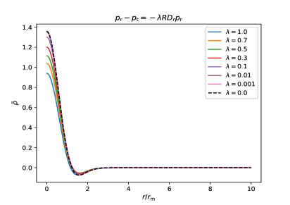
Figure 5.2: In this figure, we show the behavior $\tilde{\rho}$ against $r/r_{\mathrm{m}}$. In the left panel we are considering negative values of the anisotropy parameter $\lambda$ whereas in the right panel we account for positive values of $\lambda$.

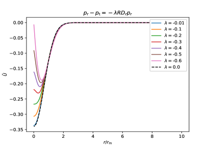
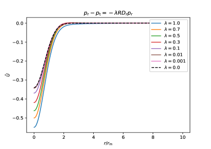
Figure 5.3: In this figure, we show the behavior of $\tilde{U}$ against $r/r_{\mathrm{m}}$. In the left panel we are considering negative values of the anisotropy parameter $\lambda$ whereas in the right panel we account for positive values of $\lambda$.

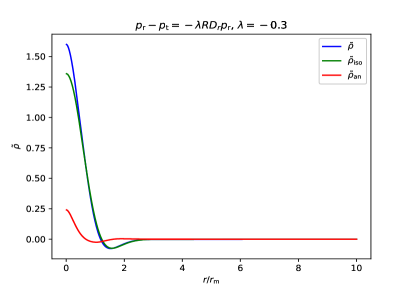
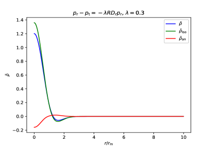
Figure 5.4: The isotropic and anisotropic contributions to the energy density perturbation. In the left panel, we show the case for $\lambda=-0.3$ whereas in the right panel we show the case for $\lambda=0.3$.

As one may see from the above figures, as $\lambda\to 0$ one can clearly see a convergence to the isotropic case and discriminate between two regimes, corresponding to positive and negative values of $\lambda$. When $\lambda<0$, given the fact that the pressure gradient profile is mainly negative, then from $p_{\mathrm{r}}-p_{\mathrm{t}}=-\lambda RD_{\mathrm{r}}p_{\mathrm{r}}$, one has that $p_{\mathrm{r}}<p_{\mathrm{t}}$. In this case, since the radial pressure is reduced compared to the tangential one, one would expect to be easier for a cosmological perturbation to collapse along the radial direction with respect to what one has in the isotropic case. Consistently, one sees that the peaks of the energy density and velocity perturbations are enhanced compared to the case when $\lambda=0$. This behavior can be clearly seen from Fig. 5.1 and Fig. 5.3. On the other hand, when $\lambda>0$, we have $p_{\mathrm{r}}>p_{\mathrm{t}}$ with this larger value of the radial component of the pressure acting against the gravitational collapse compared to the isotropic case. In this case, the amplitude of the energy density and velocity perturbations are therefore reduced with respect to the isotropic ones [See Fig. 5.1 and Fig. 5.3].

To see this effect more explicitly, we consider a positive and a negative value of $\lambda$, displaying the isotropic and the anisotropic contributions of the energy density perturbation profile in Fig. 5.4. As it can be seen from this figure, when $\lambda=-0.3$ the anisotropy has a positive contribution to the overall amplitude of the energy density perturbation, enhancing it with respect to the isotropic case. On the other hand, when $\lambda=0.3$, the anisotropic contribution reduces the amplitude of the energy density perturbation.

Finally, one should also notice from the left panel of Fig. 5.1 that for a value of $\lambda$ which is smaller than a critical value, the pressure gradient profile does not converge to zero at the origin as expected from the boundary condition given by Eq. (5.17). This behavior is explained in detail in Appendix A.3, where one can see that due to the mathematical structure of Eq. (5.57), the radial derivative of $\tilde{p}_{\mathrm{r}}$ diverges at $r=0$ when $\lambda<\lambda_{\mathrm{c}}=-9/14$.

5.5.1.2 $f(r,t)=\rho^{n}(r,t)$

We are going to consider now the EoS when $f(r,t)=\rho^{n}(r,t)$, as given by Eq. (5.20). The only difference compared to the case where $f(r,t)=R(r,t)$ is at the level of the differential equation for $\tilde{A}$ and $\tilde{p_{\mathrm{r}}}-\tilde{\rho}$. In particular, one finds that

$$\tilde{A}^{\prime} = -\frac{1}{4}\tilde{p}^{\prime}_{\mathrm{r}}\left[1-\frac{2\lambda\rho^{n}_{\mathrm{b}}}{ar}\mathchoice{{\hbox{$\displaystyle\sqrt{1-K(r)r^{2}\,}$}\lower 0.4pt\hbox{\vrule height=7.5pt,depth=-6.00003pt}}}{{\hbox{$\textstyle\sqrt{1-K(r)r^{2}\,}$}\lower 0.4pt\hbox{\vrule height=7.5pt,depth=-6.00003pt}}}{{\hbox{$\scriptstyle\sqrt{1-K(r)r^{2}\,}$}\lower 0.4pt\hbox{\vrule height=5.25pt,depth=-4.20003pt}}}{{\hbox{$\scriptscriptstyle\sqrt{1-K(r)r^{2}\,}$}\lower 0.4pt\hbox{\vrule height=3.75pt,depth=-3.00002pt}}}\right]$$ (5.60)

$$\tilde{p}_{\mathrm{r}}-\tilde{\rho} = -\frac{2\lambda\rho^{n}_{\mathrm{b}}}{3ar_{\mathrm{m}}}\mathchoice{{\hbox{$\displaystyle\sqrt{1-K(r)r^{2}\,}$}\lower 0.4pt\hbox{\vrule height=7.5pt,depth=-6.00003pt}}}{{\hbox{$\textstyle\sqrt{1-K(r)r^{2}\,}$}\lower 0.4pt\hbox{\vrule height=7.5pt,depth=-6.00003pt}}}{{\hbox{$\scriptstyle\sqrt{1-K(r)r^{2}\,}$}\lower 0.4pt\hbox{\vrule height=5.25pt,depth=-4.20003pt}}}{{\hbox{$\scriptscriptstyle\sqrt{1-K(r)r^{2}\,}$}\lower 0.4pt\hbox{\vrule height=3.75pt,depth=-3.00002pt}}}\tilde{p_{\mathrm{r}}}^{\prime}=-\frac{2\lambda\rho^{n}_{\mathrm{b}}}{3ar_{\mathrm{m}}}rH^{\prime}(r),$$ (5.61)

where

$$H(r)\equiv r_{\mathrm{m}}\int_{0}^{r}\frac{\mathchoice{{\hbox{$\displaystyle\sqrt{1-K(r^{\prime})r^{\prime 2}\,}$}\lower 0.4pt\hbox{\vrule height=7.5pt,depth=-6.00003pt}}}{{\hbox{$\textstyle\sqrt{1-K(r^{\prime})r^{\prime 2}\,}$}\lower 0.4pt\hbox{\vrule height=7.5pt,depth=-6.00003pt}}}{{\hbox{$\scriptstyle\sqrt{1-K(r^{\prime})r^{\prime 2}\,}$}\lower 0.4pt\hbox{\vrule height=5.25pt,depth=-4.20003pt}}}{{\hbox{$\scriptscriptstyle\sqrt{1-K(r^{\prime})r^{\prime 2}\,}$}\lower 0.4pt\hbox{\vrule height=3.75pt,depth=-3.00002pt}}}}{r^{\prime}}\tilde{p_{\mathrm{r}}}^{\prime}(r^{\prime})\mathrm{d}r^{\prime}.$$ (5.63)

Following the same reasoning as before one obtains for $\tilde{A}$ that

$$\tilde{A}=-\frac{\tilde{\rho}}{4}+\frac{\lambda\rho^{n}_{\mathrm{b}}}{2ar_{\mathrm{m}}}\left[\mathcal{H}(r)+\frac{r}{3}\mathcal{H}^{\prime}(r)\right],$$ (5.64)

where $\mathcal{H}(r)$ is defined as

$$\mathcal{H}(r)\equiv-r_{\mathrm{m}}\int_{r}^{\infty}\frac{\mathchoice{{\hbox{$\displaystyle\sqrt{1-K(r^{\prime})r^{\prime 2}\,}$}\lower 0.4pt\hbox{\vrule height=7.5pt,depth=-6.00003pt}}}{{\hbox{$\textstyle\sqrt{1-K(r^{\prime})r^{\prime 2}\,}$}\lower 0.4pt\hbox{\vrule height=7.5pt,depth=-6.00003pt}}}{{\hbox{$\scriptstyle\sqrt{1-K(r^{\prime})r^{\prime 2}\,}$}\lower 0.4pt\hbox{\vrule height=5.25pt,depth=-4.20003pt}}}{{\hbox{$\scriptscriptstyle\sqrt{1-K(r^{\prime})r^{\prime 2}\,}$}\lower 0.4pt\hbox{\vrule height=3.75pt,depth=-3.00002pt}}}}{r^{\prime}}\tilde{p_{\mathrm{r}}}^{\prime}(r^{\prime})\mathrm{d}r^{\prime}.$$ (5.65)

Considering $\tilde{M}$, by plugging Eq. (5.37) and Eq. (5.64) into Eq. (5.36) and taking into account Eq. (5.61) one finds that $\tilde{M}$ satisfies the following differential equation:

$$\tilde{M}+\frac{1}{3}\frac{\partial\tilde{M}}{\partial N}=\frac{2}{3}K(r)r^{2}_{\mathrm{m}}-\frac{2\lambda}{3}\frac{\rho^{n}_{\mathrm{b}}(N)}{a(N)r_{\mathrm{m}}}\mathcal{H}(r).$$ (5.66)

From the above equation, given the time-dependence of the right-hand side, one can separate the variables $(r,N)$ and the explicit profile of $\tilde{M}$ can be recast in the following way:

$$\tilde{M}=\frac{2}{3}K(r)r^{2}_{\mathrm{m}}+\Phi_{p_{\mathrm{r}}}(N)\mathcal{H}(r),$$ (5.67)

where the time-dependent function $\Phi_{p_{\mathrm{r}}}(N)$ obeys the following equation:

$$\Phi_{p_{\mathrm{r}}}^{\prime}(N)+3\Phi_{p_{\mathrm{r}}}(N)=-2\lambda\frac{\rho^{n}_{\mathrm{b}}(N)}{a(N)r_{\mathrm{m}}}.$$ (5.68)

At this point, one should stress out that $\tilde{M}$ written in the form of Eq. (5.67) is the sum of a time-independent isotropic term, $\frac{2}{3}K(r)r^{2}_{\mathrm{m}}$, plus a time-dependent anisotropic one, $\Phi_{p_{\mathrm{r}}}(N)\mathcal{H}(r)$. The differential equation for $\Phi_{p_{\mathrm{r}}}$ can be integrated analytically and it has the following solution:

$$\Phi_{p_{\mathrm{r}}}(N)=e^{-3N}\left[c-\frac{\lambda\rho^{n}_{\mathrm{b,ini}}}{a_{\mathrm{ini}}r_{\mathrm{m}}(1-2n)}e^{-(4n-2)N}\right].$$ (5.69)

By demanding that $\Phi_{p_{\mathrm{r}}}(N=0)=0$, since one expects that at initial time the anisotropy vanishes, one gets that $c=\frac{\lambda\rho^{n}_{\mathrm{b,ini}}}{a_{\mathrm{ini}}r_{\mathrm{m}}(1-2n)}$. Here one should notice that $a=a_{\mathrm{ini}}\Leftrightarrow N=0$ corresponds to an initial time when the perturbations are generated and at which one can consider that the medium is still isotropic as one expects at the end of inflation Thus, hereafter we consider that $a_{\mathrm{ini}}=a_{\mathrm{inf}}$ . At the end, taking into account the definition of $N=\ln\left(a/a_{\mathrm{ini}}\right)$ measuring the number of e-folds, $\Phi_{p_{\mathrm{r}}}$ can be written in terms of the scale factor $a$ as

$$\Phi_{p_{\mathrm{r}}}(a)=\frac{\lambda\rho^{n}_{\mathrm{b,inf}}}{a_{\mathrm{inf}}r_{\mathrm{m}}(1-2n)}\left(\frac{a}{a_{\mathrm{inf}}}\right)^{-3}\left[1-\left(\frac{a}{a_{\mathrm{inf}}}\right)^{-(4n-2)}\right],$$ (5.70)

where the index “$\mathrm{inf}$” stands for the time at the end of inflation. From Eq. (5.70) one may say that for $n=1/2$ there is an indefinite value for $\Phi_{p_{\mathrm{r}}}$ of the form $(0/0)$. However, this is not the case as one can see in Appendix A.4 in which we give $\Phi_{p_{\mathrm{r}}}$ in the limit $n\rightarrow 1/2$.

Consequently, plugging Eq. (5.67) into Eq. (5.34) and Eq. (5.37), one obtains for the energy density, velocity and lapse perturbations the following form:

$$\tilde{\rho} =\Phi_{\mathrm{iso}}\frac{1}{3r^{2}}\left[r^{3}K(r)\right]^{\prime}r^{2}_{\mathrm{m}}+\Phi_{p_{\mathrm{r}}}(a)\frac{1}{3r^{2}}\left[r^{3}\mathcal{H}(r)\right]^{\prime}$$ (5.71)

$$\tilde{U} =\frac{1}{2}\left[\left(\Phi_{\mathrm{iso}}-1\right)K(r)r^{2}_{\mathrm{m}}+\Phi_{p_{\mathrm{r}}}(a)\mathcal{H}(r)\right]$$ (5.72)

$$\tilde{A} =-\frac{1}{4}\left\{\Phi_{\mathrm{iso}}\frac{1}{3r^{2}}\left[r^{3}K(r)\right]^{\prime}r^{2}_{\mathrm{m}}+\Phi_{p_{\mathrm{r}}}(a)\frac{1}{3r^{2}}\left[r^{3}\mathcal{H}(r)\right]^{\prime}\right\}+\frac{\lambda\rho^{n}_{\mathrm{b}}(a)}{2ar_{\mathrm{m}}}\frac{\left[r^{3}\mathcal{H}(r)\right]^{\prime}}{3r^{2}},$$ (5.73)

where $\Phi_{\mathrm{iso}}=2/3$ and one can clearly identify the isotropic and anisotropic contributions.

Considering now the behavior of $\tilde{R}$ and $\tilde{B}$, by plugging Eq. (5.73) and Eq. (5.72) into Eq. (5.30) and Eq. (5.31) one gets the following differential equations for $\tilde{R}$ and $\tilde{B}$.

$$\begin{split}2\tilde{R}+\frac{\partial\tilde{R}}{\partial N}&=-\frac{\Phi_{\mathrm{iso}}}{4}\frac{1}{3r^{2}}\left[r^{3}K(r)\right]^{\prime}r^{2}_{\mathrm{m}}+\left(\Phi_{\mathrm{iso}}-1\right)\frac{K(r)r^{2}_{\mathrm{m}}}{2}\\ &-\left[\frac{\Phi_{p_{\mathrm{r}}}(N)}{4}-\frac{\lambda\rho^{n}_{\mathrm{b}}(N)}{2a(N)r_{\mathrm{m}}}\right]\frac{\left[r^{3}\mathcal{H}(r)\right]^{\prime}}{3r^{2}}+\frac{\Phi_{p_{\mathrm{r}}}(N)}{2}\mathcal{H}(r)\end{split}$$ (5.74)

$$\begin{split}2\tilde{B}+\frac{\partial\tilde{B}}{\partial N}&=\frac{r}{4}\Phi_{\mathrm{iso}}\left\{\frac{1}{3r^{2}}\left[r^{3}K(r)\right]^{\prime}r^{2}_{\mathrm{m}}\right\}^{\prime}+r\left[\frac{\Phi_{p_{\mathrm{r}}}(N)}{4}-\frac{\lambda\rho^{n}_{\mathrm{b}}(N)}{2a(N)r_{\mathrm{m}}}\right]\left\{\frac{1}{3r^{2}}\left[r^{3}\mathcal{H}(r)\right]^{\prime}\right\}^{\prime}.\end{split}$$ (5.75)

The above system of equations can be solved defining two new free functions $I_{1,p_{\mathrm{r}}}(N)$ and $I_{2,p_{\mathrm{r}}}(N)$ and writing the solutions for $\tilde{R}$ and $\tilde{B}$ as following:

$$\tilde{R} =-I_{1,\mathrm{iso}}\frac{1}{3r^{2}}\left[r^{3}K(r)\right]^{\prime}r^{2}_{\mathrm{m}}+I_{2,\mathrm{iso}}\frac{K(r)r^{2}_{\mathrm{m}}}{2}-I_{1,p_{\mathrm{r}}}(N)\frac{\left[r^{3}\mathcal{H}(r)\right]^{\prime}}{3r^{2}}+I_{2,p_{\mathrm{r}}}(N)\mathcal{H}(r)$$ (5.76)

$$\tilde{B} =I_{1,\mathrm{iso}}r\left\{\frac{1}{3r^{2}}\left[r^{3}K(r)\right]^{\prime}r^{2}_{\mathrm{m}}\right\}^{\prime}+I_{1,p_{\mathrm{r}}}(N)r\left\{\frac{\left[r^{3}\mathcal{H}(r)\right]^{\prime}}{3r^{2}}\right\}^{\prime},$$ (5.77)

where $I_{1,\mathrm{iso}}=1/12$ and $I_{2,\mathrm{iso}}=-1/6$. By plugging now Eq. (5.76) and Eq. (5.77) into Eq. (5.74) and Eq. (5.75) one obtains the differential equations for $I_{1,p_{\mathrm{r}}}(N)$ and $I_{2,p_{\mathrm{r}}}(N)$ which read as

$$I^{\prime}_{1,p_{\mathrm{r}}}(N)+2I_{1,p_{\mathrm{r}}}(N) =\frac{\Phi_{p_{\mathrm{r}}}(N)}{4}-\frac{\lambda\rho^{n}_{\mathrm{b}}(N)}{2a(N)r_{\mathrm{m}}}$$ (5.78)

$$I^{\prime}_{2,p_{\mathrm{r}}}(N)+2I_{2,p_{\mathrm{r}}}(N) =\frac{\Phi_{p_{\mathrm{r}}}(N)}{2}.$$ (5.79)

The above equations can be solved analytically imposing the initial conditions $I_{1,p_{\mathrm{r}}}(N=0)=I_{2,p_{\mathrm{r}}}(N=0)=0$ and their solutions in terms of the scale factor $a$ read as

$$\begin{split}I_{1,p_{\mathrm{r}}}(a)&=\frac{\lambda\rho^{n}_{\mathrm{b,ini}}}{4a_{\mathrm{inf}}r_{\mathrm{m}}(2n-1)(4n-1)}\left(\frac{a}{a_{\mathrm{inf}}}\right)^{-3}\\ &\times\left[4n-1+4(1-2n)\frac{a}{a_{\mathrm{inf}}}-(4n-3)\left(\frac{a}{a_{\mathrm{inf}}}\right)^{-(4n-2)}\right]\end{split}$$ (5.80)

$$I_{2,p_{\mathrm{r}}}(a) =-\frac{\lambda\rho^{n}_{\mathrm{b,inf}}}{2a_{\mathrm{ini}}r_{\mathrm{m}}(2n-1)(4n-1)}\left(\frac{a}{a_{\mathrm{inf}}}\right)^{-3}\left[1-4n+2(2n-1)\frac{a}{a_{\mathrm{inf}}}+\left(\frac{a}{a_{\mathrm{inf}}}\right)^{-(4n-2)}\right].$$ (5.81)

Interestingly, here as well, when $n=1/2$ and $n=1/4$, the behavior $I_{1,p_{\mathrm{r}}}$ and $I_{2}$ should be treated carefully. For this reason, we take the corresponding limits as it can be seen in Appendix A.4

Finally, in order to determine explicitly the initial conditions for the hydrodynamic and metric perturbations one should compute the modulating function $\mathcal{H}(r)$, which is analogous to function $\mathcal{F}(r)$ defined earlier.To do so, one can combine Eq. (5.61) and Eq. (5.71) and obtain after a straightforward calculation the following differential equation for the rescaled pressure gradient profile $h(r)$:

$$\begin{aligned} \mathchoice{{\hbox{$\displaystyle\sqrt{1-K(r)r^{2}\,}$}\lower 0.4pt\hbox{\vrule height=7.5pt,depth=-6.00003pt}}}{{\hbox{$\textstyle\sqrt{1-K(r)r^{2}\,}$}\lower 0.4pt\hbox{\vrule height=7.5pt,depth=-6.00003pt}}}{{\hbox{$\scriptstyle\sqrt{1-K(r)r^{2}\,}$}\lower 0.4pt\hbox{\vrule height=5.25pt,depth=-4.20003pt}}}{{\hbox{$\scriptscriptstyle\sqrt{1-K(r)r^{2}\,}$}\lower 0.4pt\hbox{\vrule height=3.75pt,depth=-3.00002pt}}}\left[\frac{2\lambda\rho^{n}_{\mathrm{b}}(a_{0})}{3a_{0}r_{\mathrm{m}}}-\frac{\Phi_{p_{\mathrm{r}}}(a_{0})}{3}\right]rh^{\prime}(r)&+\left\{\left[\frac{2\lambda\rho^{n}_{\mathrm{b}}(a_{0})}{3a_{0}r_{\mathrm{m}}}-\frac{4\Phi_{p_{\mathrm{r}}}(a_{0})}{3}\right]\mathchoice{{\hbox{$\displaystyle\sqrt{1-K(r)r^{2}\,}$}\lower 0.4pt\hbox{\vrule height=7.5pt,depth=-6.00003pt}}}{{\hbox{$\textstyle\sqrt{1-K(r)r^{2}\,}$}\lower 0.4pt\hbox{\vrule height=7.5pt,depth=-6.00003pt}}}{{\hbox{$\scriptstyle\sqrt{1-K(r)r^{2}\,}$}\lower 0.4pt\hbox{\vrule height=5.25pt,depth=-4.20003pt}}}{{\hbox{$\scriptscriptstyle\sqrt{1-K(r)r^{2}\,}$}\lower 0.4pt\hbox{\vrule height=3.75pt,depth=-3.00002pt}}}+r\right\}h(r)\\ &-\Phi_{\mathrm{iso}}\left[\frac{\left(r^{3}K(r)\right)^{\prime}}{3r^{2}}\right]^{\prime}r^{2}_{\mathrm{m}}\mathchoice{{\hbox{$\displaystyle\sqrt{1-K(r)r^{2}\,}$}\lower 0.4pt\hbox{\vrule height=7.5pt,depth=-6.00003pt}}}{{\hbox{$\textstyle\sqrt{1-K(r)r^{2}\,}$}\lower 0.4pt\hbox{\vrule height=7.5pt,depth=-6.00003pt}}}{{\hbox{$\scriptstyle\sqrt{1-K(r)r^{2}\,}$}\lower 0.4pt\hbox{\vrule height=5.25pt,depth=-4.20003pt}}}{{\hbox{$\scriptscriptstyle\sqrt{1-K(r)r^{2}\,}$}\lower 0.4pt\hbox{\vrule height=3.75pt,depth=-3.00002pt}}}=0\end{aligned},$$ (5.82)

where $h(r)\equiv r_{\mathrm{m}}\frac{\partial\tilde{p}_{\mathrm{r}}}{\partial r}\frac{\mathchoice{{\hbox{$\displaystyle\sqrt{1-K(r)r^{2}\,}$}\lower 0.4pt\hbox{\vrule height=5.25pt,depth=-4.20003pt}}}{{\hbox{$\textstyle\sqrt{1-K(r)r^{2}\,}$}\lower 0.4pt\hbox{\vrule height=5.25pt,depth=-4.20003pt}}}{{\hbox{$\scriptstyle\sqrt{1-K(r)r^{2}\,}$}\lower 0.4pt\hbox{\vrule height=3.67499pt,depth=-2.94pt}}}{{\hbox{$\scriptscriptstyle\sqrt{1-K(r)r^{2}\,}$}\lower 0.4pt\hbox{\vrule height=2.625pt,depth=-2.10002pt}}}}{r}$ and the anisotropy modulating terms $\Phi_{p_{\mathrm{r}}}$ and $\frac{\lambda\rho^{n}_{\mathrm{b}}(a)}{ar_{\mathrm{m}}}$ should be computed at an initial time when the gradient expansion is still valid up to a certain order $\epsilon_{0}=\epsilon(t_{0})$. The above differential equation should satisfy the analogous to $\mathcal{F}(r)$ boundary condition $\lim_{r\rightarrow 0}h(r)=0$ as imposed by Eq. (5.17). Therefore, one can solve the above differential equation for the rescaled pressure gradient profile $h(r)$, and then integrate it in order to compute $\mathcal{H}(r)$ which can be finally inserted into Eq. (5.71), Eq. (5.72), Eq. (5.73), Eq. (5.76) and Eq. (5.77) to obtain the full expressions of the initial conditions for the hydrodynamic and metric perturbations.

At this point, given the value of $n$, one can define a new dimensionless anisotropy parameter $\tilde{\lambda}$ as

$$\tilde{\lambda}=\frac{\lambda\rho^{n}_{\mathrm{b,inf}}}{r_{\mathrm{m}}},$$ (5.83)

where $\rho_{\mathrm{b,inf}}$ is the background energy density the end of inflation. With the above definition of the anisotropy parameter, the equation of state (5.20) can be recast as

$$p_{\mathrm{r}}=\frac{1}{3}\left[\rho-2\tilde{\lambda}r_{\mathrm{m}}\left(\frac{\rho}{\rho_{\mathrm{b,inf}}}\right)^{n}D_{\mathrm{r}}p_{\mathrm{r}}\right].$$ (5.84)

We should also stress out here that our problem at hand requires to specify five input parameters in order to fully specify the initial conditions for the hydrodynamic and metric perturbations. In particular, these parameters are a) the index $n$ appearing in the equation of state Eq. (5.84), b) the dimensionless anisotropy parameter $\tilde{\lambda}$, c) the ratio between the energy scales at horizon crossing ($\epsilon_{\mathrm{HC}}=1$) and the energy scale at the end of inflation, i.e. $q=\left(\frac{\rho_{\mathrm{b,HC}}}{\rho_{\mathrm{b,inf}}}\right)^{1/4}$, d) the small initial parameter $\epsilon_{0}=\frac{H^{-1}_{0}}{a_{\mathrm{0}}r_{\mathrm{m}}}$ and e) the background energy density, $\rho_{\mathrm{b,inf}}$, measured at the end of inflation, which depends on the underlying inflationary model generating the hydrodynamic and metric perturbations. At the end, the initial conditions for $\tilde{A}$, $\tilde{R}$, $\tilde{B}$, $\tilde{M}$, $\tilde{\rho}$ and $\tilde{U}$ could be written in a compact form as follows:

$$\begin{split}\tilde{M}&=\frac{2}{3}K(r)r^{2}_{\mathrm{m}}+\Phi_{p_{\mathrm{r}}}(N)\mathcal{H}(r)\\ \tilde{\rho}&=\Phi_{\mathrm{iso}}\frac{1}{3r^{2}}\left[r^{3}K(r)\right]^{\prime}r^{2}_{\mathrm{m}}+\Phi_{p_{\mathrm{r}}}(a_{0})\frac{1}{3r^{2}}\left[r^{3}\mathcal{H}(r)\right]^{\prime}\\ \tilde{U}&=\frac{1}{2}\left[\left(\Phi_{\mathrm{iso}}-1\right)K(r)r^{2}_{\mathrm{m}}+\Phi_{p_{\mathrm{r}}}(a_{0})\mathcal{H}(r)\right]\\ \tilde{A}&=-\frac{1}{4}\left\{\Phi_{\mathrm{iso}}\frac{1}{3r^{2}}\left[r^{3}K(r)\right]^{\prime}r^{2}_{\mathrm{m}}+\Phi_{p_{\mathrm{r}}}(a_{0})\frac{1}{3r^{2}}\left[r^{3}\mathcal{H}(r)\right]^{\prime}\right\}+\frac{\lambda\rho^{n}_{\mathrm{b}}(a_{0})}{2a_{0}r_{\mathrm{m}}}\frac{\left[r^{3}\mathcal{H}(r)\right]^{\prime}}{3r^{2}}\\ \tilde{R}&=-I_{1,\mathrm{iso}}\frac{1}{3r^{2}}\left[r^{3}K(r)\right]^{\prime}r^{2}_{\mathrm{m}}+I_{2,\mathrm{iso}}\frac{K(r)r^{2}_{\mathrm{m}}}{2}-I_{1,p_{\mathrm{r}}}(a_{0})\frac{\left[r^{3}\mathcal{H}(r)\right]^{\prime}}{3r^{2}}+I_{2,p_{\mathrm{r}}}(a_{0})\mathcal{H}(r)\\ \tilde{B}&=I_{1,\mathrm{iso}}r\left\{\frac{1}{3r^{2}}\left[r^{3}K(r)\right]^{\prime}r^{2}_{\mathrm{m}}\right\}^{\prime}+I_{1,p_{\mathrm{r}}}(a_{0})r\left\{\frac{\left[r^{3}\mathcal{H}(r)\right]^{\prime}}{3r^{2}}\right\}^{\prime},\end{split}$$ (5.85)

where the modulating functions $\Phi_{p_{\mathrm{r}}}$, $\frac{\lambda\rho^{n}_{\mathrm{b}}(a)}{ar_{\mathrm{m}}}$, $I_{1,p_{\mathrm{r}}}$ and $I_{2,p_{\mathrm{r}}}$ should be computed at initial time $t_{0}$ when the gradient expansion is valid up to a certain order $\epsilon_{0}$. Below, we give their explicit dependence on $q$, $\epsilon_{0}$, $n$ and $\tilde{\lambda}$.

$$\frac{\lambda\rho^{n}_{\mathrm{b}}(a_{0})}{a_{0}r_{\mathrm{m}}} =\frac{\tilde{\lambda}}{q}\left(\frac{q}{\epsilon_{0}}\right)^{4n+1}$$ (5.86)

$$\Phi_{p_{\mathrm{r}}}(a_{0}) =\frac{\tilde{\lambda}}{q(1-2n)}\left(\frac{q}{\epsilon_{0}}\right)^{3}\left[1-\left(\frac{q}{\epsilon_{0}}\right)^{(4n-2)}\right]$$ (5.87)

$$\begin{split}I_{1,p_{\mathrm{r}}}(a_{0})&=\frac{\tilde{\lambda}}{4q(2n-1)(4n-1)}\left(\frac{q}{\epsilon_{0}}\right)^{3}\\ &\times\left[4n-1+4(1-2n)\frac{\epsilon_{0}}{q}-(4n-3)\left(\frac{q}{\epsilon_{0}}\right)^{(4n-2)}\right]\end{split}$$ (5.88)

$$I_{2,p_{\mathrm{r}}}(a_{0}) =-\frac{\tilde{\lambda}}{2q(2n-1)(4n-1)}\left(\frac{q}{\epsilon_{0}}\right)^{3}\left[1-4n+2(2n-1)\frac{\epsilon_{0}}{q}+\left(\frac{q}{\epsilon_{0}}\right)^{(4n-2)}\right].$$ (5.89)

Here, one should point out that at the level of the equation of state we identify three main contributions. First, the dimensionless parameter $\tilde{\lambda}$ accounting for the anisotropy of the medium. Second, the ratio $\left(\frac{\rho}{\rho_{\mathrm{b,inf}}}\right)^{n}$ which is measuring for the effect of cosmic expansion and finally the term $D_{\mathrm{r}}p_{\mathrm{r}}$ which accounts for the effect of the pressure gradients. Regarding the possible values of $n$, one can assume based on physical arguments that at the infinite time limit the pressure gradient contributions disappear, implying that $n\geq 0$. The values of the anisotropic parameter $\tilde{\lambda}$ can in principle take any value.

In the following figures, we show the behavior of the initial conditions of the pressure gradients, the energy density and velocity perturbations for a specific toy-model, i.e. $n=0$, considering positive values of the dimensionless anisotropy parameter $\tilde{\lambda}$ and taking into account that, due to the structure of Eq. (5.82) which describes the behavior of the pressure gradients, one is facing a divergence at $r=0$ for negative values of $\tilde{\lambda}$. [See also the discussion in Appendix A.3.]

As it can be seen from the figures below,where we choose $q=10^{-10}$ and $\epsilon_{0}=10^{-1}$, the behavior of the initial conditions for the hydrodynamic and metric perturbations is similar to the case where $f(r,t)=R(r,t)$ with a positive value of $\tilde{\lambda}$ enhancing the radial pressure compared to the tangential one and leading to a lower amplitude of the matter perturbations $\tilde{\rho}$ and $\tilde{U}$ with respect to the isotropic case [See Fig. 5.6].

Figure 5.5: In this figure, we plot $\frac{\partial\tilde{p}_{\mathrm{r}}}{\partial r}$ against $r/r_{\mathrm{m}}$ by considering positive values of $\tilde{\lambda}$. We have chosen $n=0$, $q=10^{-10}$ and $\epsilon_{0}=10^{-1}$.

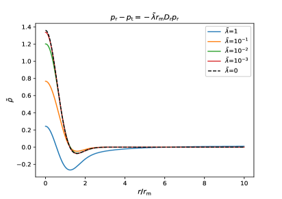
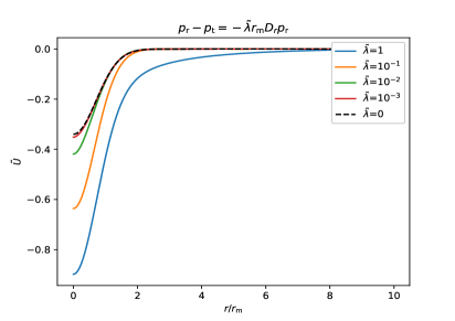
Figure 5.6: In the left panel we show $\tilde{\rho}$ against $r/r_{\mathrm{m}}$ for different values of $\tilde{\lambda}>0$ while in the right one we show $\tilde{U}$ against $r/r_{\mathrm{m}}$, considering different values of $\tilde{\lambda}>0$. We have chosen $n=0$, $q=10^{-10}$ and $\epsilon_{0}=10^{-1}$.

5.5.2 Equation of state in terms of energy density gradients

We study here the quasi-homogeneous solution when the EoS is given by Eq. (5.16), where the function $f(r,t)$ is chosen to be either $f(r,t)=R(r,t)$ or $f(r,t)=\rho^{n}(r,t)$.

5.5.2.1 $f(r,t)=R(r,t)$

Following the same reasoning as before, the only place in which we see a difference compared to the previous cases is in the differential equations for $\tilde{A}$ and $\tilde{p}_{\mathrm{r}}-\tilde{\rho}$ which now read as

$$\tilde{A}^{\prime} = -\frac{1}{4}\left[\tilde{p}^{\prime}_{\mathrm{r}}-6\lambda\mathchoice{{\hbox{$\displaystyle\sqrt{1-K(r)r^{2}\,}$}\lower 0.4pt\hbox{\vrule height=7.5pt,depth=-6.00003pt}}}{{\hbox{$\textstyle\sqrt{1-K(r)r^{2}\,}$}\lower 0.4pt\hbox{\vrule height=7.5pt,depth=-6.00003pt}}}{{\hbox{$\scriptstyle\sqrt{1-K(r)r^{2}\,}$}\lower 0.4pt\hbox{\vrule height=5.25pt,depth=-4.20003pt}}}{{\hbox{$\scriptscriptstyle\sqrt{1-K(r)r^{2}\,}$}\lower 0.4pt\hbox{\vrule height=3.75pt,depth=-3.00002pt}}}\tilde{\rho}^{\prime}\right]$$ (5.90)

$$\tilde{p}_{\mathrm{r}}-\tilde{\rho} = -2\lambda r\mathchoice{{\hbox{$\displaystyle\sqrt{1-K(r)r^{2}\,}$}\lower 0.4pt\hbox{\vrule height=7.5pt,depth=-6.00003pt}}}{{\hbox{$\textstyle\sqrt{1-K(r)r^{2}\,}$}\lower 0.4pt\hbox{\vrule height=7.5pt,depth=-6.00003pt}}}{{\hbox{$\scriptstyle\sqrt{1-K(r)r^{2}\,}$}\lower 0.4pt\hbox{\vrule height=5.25pt,depth=-4.20003pt}}}{{\hbox{$\scriptscriptstyle\sqrt{1-K(r)r^{2}\,}$}\lower 0.4pt\hbox{\vrule height=3.75pt,depth=-3.00002pt}}}\tilde{\rho}^{\prime}=-2\lambda rG^{\prime}(r),$$ (5.91)

where

$$G(r)\equiv\int_{0}^{r}\mathchoice{{\hbox{$\displaystyle\sqrt{1-K(r^{\prime})r^{\prime 2}\,}$}\lower 0.4pt\hbox{\vrule height=7.5pt,depth=-6.00003pt}}}{{\hbox{$\textstyle\sqrt{1-K(r^{\prime})r^{\prime 2}\,}$}\lower 0.4pt\hbox{\vrule height=7.5pt,depth=-6.00003pt}}}{{\hbox{$\scriptstyle\sqrt{1-K(r^{\prime})r^{\prime 2}\,}$}\lower 0.4pt\hbox{\vrule height=5.25pt,depth=-4.20003pt}}}{{\hbox{$\scriptscriptstyle\sqrt{1-K(r^{\prime})r^{\prime 2}\,}$}\lower 0.4pt\hbox{\vrule height=3.75pt,depth=-3.00002pt}}}\tilde{\rho}^{\prime}(r^{\prime})\mathrm{d}r^{\prime}.$$ (5.92)

Then, in order to put the expressions for $\tilde{A}$, $\tilde{R}$, $\tilde{B}$, $\tilde{M}$, $\tilde{\rho}$ and $\tilde{U}$ in a compact form as in Sec. 5.5.1.1, we introduce an effective curvature profile similar to the one defined in Eq. (5.52) as follows:

$$\mathcal{K}(r)=K(r)-\frac{3\lambda}{r^{2}_{\mathrm{m}}}\mathcal{G}(r),$$ (5.93)

where

$$\mathcal{G}(r)\equiv G(r)-G(\infty)=-\int_{r}^{\infty}\frac{\partial\tilde{\rho}(r^{\prime})}{\partial r^{\prime}}\mathchoice{{\hbox{$\displaystyle\sqrt{1-K(r^{\prime})r^{\prime 2}\,}$}\lower 0.4pt\hbox{\vrule height=7.5pt,depth=-6.00003pt}}}{{\hbox{$\textstyle\sqrt{1-K(r^{\prime})r^{\prime 2}\,}$}\lower 0.4pt\hbox{\vrule height=7.5pt,depth=-6.00003pt}}}{{\hbox{$\scriptstyle\sqrt{1-K(r^{\prime})r^{\prime 2}\,}$}\lower 0.4pt\hbox{\vrule height=5.25pt,depth=-4.20003pt}}}{{\hbox{$\scriptscriptstyle\sqrt{1-K(r^{\prime})r^{\prime 2}\,}$}\lower 0.4pt\hbox{\vrule height=3.75pt,depth=-3.00002pt}}}\mathrm{d}r^{\prime}.$$ (5.94)

We define as well the effective energy density and velocity perturbations $\tilde{\rho}_{\mathrm{eff}}$ and $\tilde{U}_{\mathrm{eff}}$ such that the quasi-homogeneous solution is written in a similar form as in the isotropic case ($\lambda=0$),

$$\tilde{\rho}_{\mathrm{eff}}=\tilde{\rho}-2\lambda\left[r\mathcal{G}^{\prime}(r)+3\mathcal{G}(r)\right]$$ (5.95)

$$\tilde{U}_{\mathrm{eff}}=\tilde{U}+\frac{3\lambda}{2}\mathcal{G}(r)=-\frac{1}{6}\mathcal{K}(r)r^{2}_{\mathrm{m}}.$$ (5.96)

At the end, one gets the hydrodynamic and metric perturbations in the following compact form:

$$\begin{aligned} \tilde{A}&=-\frac{\tilde{\rho}}{4}+\frac{\lambda}{2}\left[r\mathcal{G}^{\prime}(r)+3\mathcal{G}(r)\right]=-\frac{\tilde{\rho}_{\mathrm{eff}}}{4}\\ \tilde{B}&=\frac{r}{8}\left[\tilde{\rho}^{\prime}-2\lambda r\mathcal{G}^{\prime\prime}(r)-8\lambda\mathcal{G}^{\prime}(r)\right]=\frac{r}{8}\tilde{\rho}^{\prime}_{\mathrm{eff}}\\ \tilde{\rho}&=\frac{2}{3}\frac{\left[r^{3}\mathcal{K}(r)\right]^{\prime}}{3r^{2}}r^{2}_{\mathrm{m}}\\ \tilde{U}&=-\frac{1}{6}\mathcal{K}(r)r_{\mathrm{m}}^{2}-\frac{3\lambda}{2}\mathcal{G}(r)=\tilde{U}_{\mathrm{eff}}-\frac{\lambda}{2}\mathcal{G}(r)\\ \tilde{M}&=\frac{2}{3}\mathcal{K}(r)r_{\mathrm{m}}^{2}=-4\tilde{U}_{\mathrm{eff}}\\ \tilde{R}&=-\frac{\tilde{\rho}_{\mathrm{eff}}}{8}+\frac{\tilde{U}}{2}\end{aligned}$$ (5.97)

Finally, in order to express explicitly the initial conditions for the hydrodynamic and metric perturbations, one should compute the behavior of the energy density gradient profile $\frac{\partial\tilde{\rho}}{\partial r}$. Combining then Eq. (5.91) and Eq. (5.34) one gets the following equation for

$$g(r)\equiv\frac{\partial\tilde{\rho}}{\partial r}\mathchoice{{\hbox{$\displaystyle\sqrt{1-K(r)r^{2}\,}$}\lower 0.4pt\hbox{\vrule height=7.5pt,depth=-6.00003pt}}}{{\hbox{$\textstyle\sqrt{1-K(r)r^{2}\,}$}\lower 0.4pt\hbox{\vrule height=7.5pt,depth=-6.00003pt}}}{{\hbox{$\scriptstyle\sqrt{1-K(r)r^{2}\,}$}\lower 0.4pt\hbox{\vrule height=5.25pt,depth=-4.20003pt}}}{{\hbox{$\scriptscriptstyle\sqrt{1-K(r)r^{2}\,}$}\lower 0.4pt\hbox{\vrule height=3.75pt,depth=-3.00002pt}}}$$

analogous to Eq. (5.57):

$$\frac{2\lambda}{3}r\mathchoice{{\hbox{$\displaystyle\sqrt{1-K(r)r^{2}\,}$}\lower 0.4pt\hbox{\vrule height=7.5pt,depth=-6.00003pt}}}{{\hbox{$\textstyle\sqrt{1-K(r)r^{2}\,}$}\lower 0.4pt\hbox{\vrule height=7.5pt,depth=-6.00003pt}}}{{\hbox{$\scriptstyle\sqrt{1-K(r)r^{2}\,}$}\lower 0.4pt\hbox{\vrule height=5.25pt,depth=-4.20003pt}}}{{\hbox{$\scriptscriptstyle\sqrt{1-K(r)r^{2}\,}$}\lower 0.4pt\hbox{\vrule height=3.75pt,depth=-3.00002pt}}}g^{\prime}(r) +\left[\frac{8\lambda}{3}\mathchoice{{\hbox{$\displaystyle\sqrt{1-K(r)r^{2}\,}$}\lower 0.4pt\hbox{\vrule height=7.5pt,depth=-6.00003pt}}}{{\hbox{$\textstyle\sqrt{1-K(r)r^{2}\,}$}\lower 0.4pt\hbox{\vrule height=7.5pt,depth=-6.00003pt}}}{{\hbox{$\scriptstyle\sqrt{1-K(r)r^{2}\,}$}\lower 0.4pt\hbox{\vrule height=5.25pt,depth=-4.20003pt}}}{{\hbox{$\scriptscriptstyle\sqrt{1-K(r)r^{2}\,}$}\lower 0.4pt\hbox{\vrule height=3.75pt,depth=-3.00002pt}}}+1\right]g(r)+$$ (5.98)

$$-\frac{2}{3}\left\{\frac{\left[r^{3}K(r)\right]^{\prime}}{3r^{2}}\right\}^{\prime}r^{2}_{\mathrm{m}}\mathchoice{{\hbox{$\displaystyle\sqrt{1-K(r)r^{2}\,}$}\lower 0.4pt\hbox{\vrule height=7.5pt,depth=-6.00003pt}}}{{\hbox{$\textstyle\sqrt{1-K(r)r^{2}\,}$}\lower 0.4pt\hbox{\vrule height=7.5pt,depth=-6.00003pt}}}{{\hbox{$\scriptstyle\sqrt{1-K(r)r^{2}\,}$}\lower 0.4pt\hbox{\vrule height=5.25pt,depth=-4.20003pt}}}{{\hbox{$\scriptscriptstyle\sqrt{1-K(r)r^{2}\,}$}\lower 0.4pt\hbox{\vrule height=3.75pt,depth=-3.00002pt}}}=0,$$

with the boundary condition $g(0)=0$. By solving for $g(r)$ the above equation, we integrate $g(r)$ in order to get the anisotropic modulating function $\mathcal{G}(r)$ modifying all the hydrodynamic and metric perturbations as one can see from Eq. (5.97).

Below, we show the energy density gradient profiles considering both positive and negative values of $\lambda$, together the behavior of the energy density and velocity perturbation’s profiles. For the figures below, we chose as before a curvature profile for $K(r)$ having a Gaussian form $K(r)=\mathcal{A}e^{-(r/r_{\mathrm{m,0}})^{2}}$ with $r_{\mathrm{m,0}}=1$ and $\mathcal{A}=\frac{3e}{4r^{2}_{\mathrm{m,0}}}$. Regarding the value of $r_{\mathrm{m}}$, we take as before $r_{\mathrm{m}}=r_{\mathrm{m,0}}=1$, since also in this case $r_{\mathrm{m}}\simeq r_{\mathrm{m,0}}$ independently of the value of $\lambda$ we have considered.

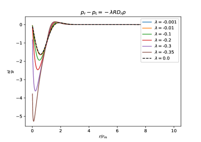
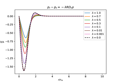
Figure 5.7: In this figure, we show the $\frac{\partial\tilde{\rho}}{\partial r}$ against $r/r_{\mathrm{m}}$. In the left panel, we consider negative values of $\lambda$ whereas in the right panel we account for positive values of $\lambda$.

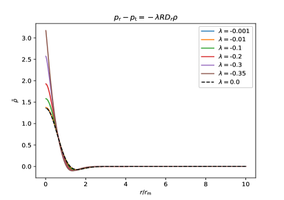
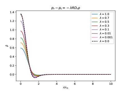
Figure 5.8: In this figure, we show the $\tilde{\rho}$ against $r/r_{\mathrm{m}}$. In the left panel, we consider negative values of $\lambda$ whereas in the right panel we account for positive values of $\lambda$.

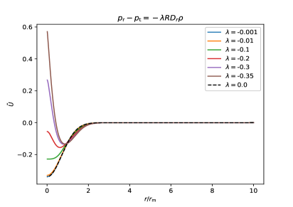
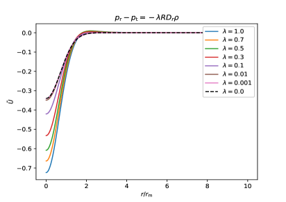
Figure 5.9: In this figure, we show the $\tilde{U}$ against $r/r_{\mathrm{m}}$. In the left panel, we consider negative values of $\lambda$ whereas in the right panel we account for positive values of $\lambda$.

As in the case where $p_{\mathrm{r}}-p_{\mathrm{t}}=-\lambda RD_{\mathrm{r}}p_{\mathrm{r}}$, we identify two regimes: a) when $\lambda<0$, characterized by the fact that $\frac{\partial\tilde{\rho}}{\partial r}$ is mainly negative and one obtains that $p_{\mathrm{r}}<p_{\mathrm{t}}$ suggesting in this way the possibility for a cosmological perturbation to collapse more easily and b) when $\lambda>0$ where $p_{\mathrm{r}}>p_{\mathrm{t}}$ and it is more difficult for a perturbation to collapse.

Regarding the behavior of the energy density gradient, similarly to the case where $p_{\mathrm{r}}-p_{\mathrm{t}}=-\lambda RD_{\mathrm{r}}p_{\mathrm{r}}$, one can identify from Fig. 5.7 a lower bound in $\lambda$, which can be explained from the mathematical structure of Eq. (5.98) describing the behavior of $\frac{\partial\tilde{\rho}}{\partial r}$. [See also the Appendix A.3].

5.5.2.2 $f(r,t)=\rho^{n}(r,t)$

We now consider the EoS with $f(r,t)=\rho^{n}(r,t)$, given by Eq. (5.21). Following the same strategy as in Sec. 5.5.1.2, the differential equations for $\tilde{A}$ and $\tilde{p}_{\mathrm{r}}-\tilde{\rho}$ read as

$$\tilde{A}^{\prime} = -\frac{1}{4}\left[\tilde{p}^{\prime}_{\mathrm{r}}-\frac{6\lambda\rho^{n}_{\mathrm{b}}}{ar}\mathchoice{{\hbox{$\displaystyle\sqrt{1-K(r)r^{2}\,}$}\lower 0.4pt\hbox{\vrule height=7.5pt,depth=-6.00003pt}}}{{\hbox{$\textstyle\sqrt{1-K(r)r^{2}\,}$}\lower 0.4pt\hbox{\vrule height=7.5pt,depth=-6.00003pt}}}{{\hbox{$\scriptstyle\sqrt{1-K(r)r^{2}\,}$}\lower 0.4pt\hbox{\vrule height=5.25pt,depth=-4.20003pt}}}{{\hbox{$\scriptscriptstyle\sqrt{1-K(r)r^{2}\,}$}\lower 0.4pt\hbox{\vrule height=3.75pt,depth=-3.00002pt}}}\tilde{\rho}^{\prime}\right]$$ (5.99)

$$\tilde{p}_{\mathrm{r}}-\tilde{\rho} = -\frac{2\lambda\rho^{n}_{\mathrm{b}}}{a}\mathchoice{{\hbox{$\displaystyle\sqrt{1-K(r)r^{2}\,}$}\lower 0.4pt\hbox{\vrule height=7.5pt,depth=-6.00003pt}}}{{\hbox{$\textstyle\sqrt{1-K(r)r^{2}\,}$}\lower 0.4pt\hbox{\vrule height=7.5pt,depth=-6.00003pt}}}{{\hbox{$\scriptstyle\sqrt{1-K(r)r^{2}\,}$}\lower 0.4pt\hbox{\vrule height=5.25pt,depth=-4.20003pt}}}{{\hbox{$\scriptscriptstyle\sqrt{1-K(r)r^{2}\,}$}\lower 0.4pt\hbox{\vrule height=3.75pt,depth=-3.00002pt}}}\tilde{\rho}^{\prime}=-\frac{2\lambda\rho^{n}_{\mathrm{b}}}{ar_{\mathrm{m}}}rJ^{\prime}(r),$$ (5.100)

where

$$J(r)\equiv r_{\mathrm{m}}\int_{0}^{r}\frac{\mathchoice{{\hbox{$\displaystyle\sqrt{1-K(r^{\prime})r^{\prime 2}\,}$}\lower 0.4pt\hbox{\vrule height=7.5pt,depth=-6.00003pt}}}{{\hbox{$\textstyle\sqrt{1-K(r^{\prime})r^{\prime 2}\,}$}\lower 0.4pt\hbox{\vrule height=7.5pt,depth=-6.00003pt}}}{{\hbox{$\scriptstyle\sqrt{1-K(r^{\prime})r^{\prime 2}\,}$}\lower 0.4pt\hbox{\vrule height=5.25pt,depth=-4.20003pt}}}{{\hbox{$\scriptscriptstyle\sqrt{1-K(r^{\prime})r^{\prime 2}\,}$}\lower 0.4pt\hbox{\vrule height=3.75pt,depth=-3.00002pt}}}}{r^{\prime}}\tilde{\rho}^{\prime}(r^{\prime})\mathrm{d}r^{\prime}.$$ (5.101)

The differential equations for $\tilde{R}$, $\tilde{B}$, $\tilde{M}$, $\tilde{\rho}$ and $\tilde{U}$, taking into account that these quantities do not depend on the prescription modeling the difference $p_{\mathrm{r}}-p_{\mathrm{t}}$, will be given by Eqs. (5.38). Integrating them using the above equations, similarly as in Sec. 5.5.1.2, one can write the profiles of $\tilde{A}$, $\tilde{R}$, $\tilde{B}$, $\tilde{M}$, $\tilde{\rho}$ and $\tilde{U}$ as follows:

$$\begin{split}\tilde{M}&=\frac{2}{3}K(r)r^{2}_{\mathrm{m}}+\Phi_{\rho}(a_{0})\mathcal{J}(r)\\ \tilde{\rho}&=\Phi_{\mathrm{iso}}\frac{1}{3r^{2}}\left[r^{3}K(r)\right]^{\prime}r^{2}_{\mathrm{m}}+\Phi_{\rho}(a_{0})\frac{1}{3r^{2}}\left[r^{3}\mathcal{J}(r)\right]^{\prime}\\ \tilde{U}&=\frac{1}{2}\left[\left(\Phi_{\mathrm{iso}}-1\right)K(r)r^{2}_{\mathrm{m}}+\Phi_{\rho}(a_{0})\mathcal{J}(r)\right]\\ \tilde{A}&=-\frac{1}{4}\left\{\Phi_{\mathrm{iso}}\frac{1}{3r^{2}}\left[r^{3}K(r)\right]^{\prime}r^{2}_{\mathrm{m}}+\Phi_{\rho}(a_{0})\frac{1}{3r^{2}}\left[r^{3}\mathcal{J}(r)\right]^{\prime}\right\}+\frac{3\lambda\rho^{n}_{\mathrm{b}}(a_{0})}{2a_{0}r_{\mathrm{m}}}\frac{\left[r^{3}\mathcal{J}(r)\right]^{\prime}}{3r^{2}}\\ \tilde{R}&=-I_{1,\mathrm{iso}}\frac{1}{3r^{2}}\left[r^{3}K(r)\right]^{\prime}r^{2}_{\mathrm{m}}+I_{2,\mathrm{iso}}\frac{K(r)r^{2}_{\mathrm{m}}}{2}-I_{1,\rho}(a_{0})\frac{\left[r^{3}\mathcal{J}(r)\right]^{\prime}}{3r^{2}}+I_{2,\rho}(a_{0})\mathcal{J}(r)\\ \tilde{B}&=I_{1,\mathrm{iso}}r\left\{\frac{1}{3r^{2}}\left[r^{3}K(r)\right]^{\prime}r^{2}_{\mathrm{m}}\right\}^{\prime}+I_{1,\rho}(a_{0})r\left\{\frac{\left[r^{3}\mathcal{J}(r)\right]^{\prime}}{3r^{2}}\right\}^{\prime},\end{split}$$ (5.102)

where $\mathcal{J}(r)$ is defined as

$$\mathcal{J}(r)\equiv-r_{\mathrm{m}}\int_{r}^{\infty}\frac{\mathchoice{{\hbox{$\displaystyle\sqrt{1-K(r^{\prime})r^{\prime 2}\,}$}\lower 0.4pt\hbox{\vrule height=7.5pt,depth=-6.00003pt}}}{{\hbox{$\textstyle\sqrt{1-K(r^{\prime})r^{\prime 2}\,}$}\lower 0.4pt\hbox{\vrule height=7.5pt,depth=-6.00003pt}}}{{\hbox{$\scriptstyle\sqrt{1-K(r^{\prime})r^{\prime 2}\,}$}\lower 0.4pt\hbox{\vrule height=5.25pt,depth=-4.20003pt}}}{{\hbox{$\scriptscriptstyle\sqrt{1-K(r^{\prime})r^{\prime 2}\,}$}\lower 0.4pt\hbox{\vrule height=3.75pt,depth=-3.00002pt}}}}{r^{\prime}}\tilde{\rho}^{\prime}(r^{\prime})\mathrm{d}r^{\prime}.$$ (5.103)

The anisotropy modulating functions $\Phi_{\rho}$, $I_{1,\rho}$ and $I_{2,\rho}$, calculated at initial time $t_{0}$ when the gradient expansion is valid up a certain order $\epsilon_{0}$, satisfy the following differential equations

$$\Phi_{\rho}^{\prime}(N)+3\Phi_{\rho}(N) =-6\lambda\frac{\rho^{n}_{\mathrm{b}}(N)}{a(N)r_{\mathrm{m}}}$$ (5.104)

$$I^{\prime}_{1,\rho}(N)+2I_{1,\rho}(N) =\frac{\Phi_{\rho}(N)}{4}-\frac{3\lambda\rho^{n}_{\mathrm{b}}(N)}{2a(N)r_{\mathrm{m}}}$$ (5.105)

$$I^{\prime}_{2,\rho}(N)+2I_{2,\rho}(N) =\frac{\Phi_{\rho}(N)}{2},$$ (5.106)

with initial conditions $\Phi(N=0)=I_{1,\rho}(N=0)=I_{2,\rho}(N=0)=0$. After solving the above differential equations, the solutions of for $\Phi_{\rho}$, $I_{1,\rho}$ and $I_{2,\rho}$ in terms of the scale factor read as

$$\Phi_{\rho}(a) =3\frac{\lambda\rho^{n}_{\mathrm{b,inf}}}{a_{\mathrm{inf}}r_{\mathrm{m}}(1-2n)}\left(\frac{a}{a_{\mathrm{inf}}}\right)^{-3}\left[1-\left(\frac{a}{a_{\mathrm{inf}}}\right)^{-(4n-2)}\right]$$ (5.107)

$$\begin{split}I_{1,\rho}(a)&=\frac{3\lambda\rho^{n}_{\mathrm{b,inf}}}{4a_{\mathrm{inf}}r_{\mathrm{m}}(2n-1)(4n-1)}\left(\frac{a}{a_{\mathrm{inf}}}\right)^{-3}\\ &\times\left[4n-1+4(1-2n)\frac{a}{a_{\mathrm{inf}}}-(4n-3)\left(\frac{a}{a_{\mathrm{inf}}}\right)^{-(4n-2)}\right]\end{split}]$$ (5.108)

$$I_{2,\rho}(a) =-\frac{3\lambda\rho^{n}_{\mathrm{b,inf}}}{2a_{\mathrm{inf}}r_{\mathrm{m}}(2n-1)(4n-1)}\left(\frac{a}{a_{\mathrm{inf}}}\right)^{-3}\left[1-4n+2(2n-1)\frac{a}{a_{\mathrm{inf}}}+\left(\frac{a}{a_{\mathrm{inf}}}\right)^{-(4n-2)}\right].$$ (5.109)

As in Sec. 5.5.1.2, $N=0$ refers to $a=a_{\mathrm{inf}}$, the time when inflation ends, corresponding to the epoch when the cosmological perturbations are generated. For this reason, when $N=0$ we are essentially still in the isotropic regime. The limits for $n\rightarrow 1/2$ and $n\rightarrow 1/4$ for the modulating functions $\Phi_{\rho}$, $I_{1,\rho}$ and $I_{2,\rho}$ are given in Appendix A.4.

Finally, in order to specify explicitly the initial conditions for the hydrodynamic and metric pertubations one should compute the energy density gradient profile, $\frac{\partial\tilde{\rho}}{\partial r}$ and then integrate it to obtain the modulating function $\mathcal{J}(r)$. Doing so, one can combine Eq. (5.100) and Eq. (5.34) and obtain after a straighforward calculation the following differential equation for the rescaled energy density gradient profile $j(r)$:

$$\begin{aligned} \frac{\Phi_{\rho}(a_{0})\mathchoice{{\hbox{$\displaystyle\sqrt{1-K(r)r^{2}\,}$}\lower 0.4pt\hbox{\vrule height=7.5pt,depth=-6.00003pt}}}{{\hbox{$\textstyle\sqrt{1-K(r)r^{2}\,}$}\lower 0.4pt\hbox{\vrule height=7.5pt,depth=-6.00003pt}}}{{\hbox{$\scriptstyle\sqrt{1-K(r)r^{2}\,}$}\lower 0.4pt\hbox{\vrule height=5.25pt,depth=-4.20003pt}}}{{\hbox{$\scriptscriptstyle\sqrt{1-K(r)r^{2}\,}$}\lower 0.4pt\hbox{\vrule height=3.75pt,depth=-3.00002pt}}}}{3}rj^{\prime}(r)&+\left\{\frac{4\Phi_{\rho}(a_{0})}{3}\mathchoice{{\hbox{$\displaystyle\sqrt{1-K(r)r^{2}\,}$}\lower 0.4pt\hbox{\vrule height=7.5pt,depth=-6.00003pt}}}{{\hbox{$\textstyle\sqrt{1-K(r)r^{2}\,}$}\lower 0.4pt\hbox{\vrule height=7.5pt,depth=-6.00003pt}}}{{\hbox{$\scriptstyle\sqrt{1-K(r)r^{2}\,}$}\lower 0.4pt\hbox{\vrule height=5.25pt,depth=-4.20003pt}}}{{\hbox{$\scriptscriptstyle\sqrt{1-K(r)r^{2}\,}$}\lower 0.4pt\hbox{\vrule height=3.75pt,depth=-3.00002pt}}}-r\right\}j(r)\\ &+\Phi_{\mathrm{iso}}\left[\frac{\left(r^{3}K(r)\right)^{\prime}}{3r^{2}}\right]^{\prime}r^{2}_{\mathrm{m}}\mathchoice{{\hbox{$\displaystyle\sqrt{1-K(r)r^{2}\,}$}\lower 0.4pt\hbox{\vrule height=7.5pt,depth=-6.00003pt}}}{{\hbox{$\textstyle\sqrt{1-K(r)r^{2}\,}$}\lower 0.4pt\hbox{\vrule height=7.5pt,depth=-6.00003pt}}}{{\hbox{$\scriptstyle\sqrt{1-K(r)r^{2}\,}$}\lower 0.4pt\hbox{\vrule height=5.25pt,depth=-4.20003pt}}}{{\hbox{$\scriptscriptstyle\sqrt{1-K(r)r^{2}\,}$}\lower 0.4pt\hbox{\vrule height=3.75pt,depth=-3.00002pt}}}=0\end{aligned},$$ (5.110)

where $j(r)\equiv r_{\mathrm{m}}\frac{\partial\tilde{\rho}}{\partial r}\frac{\mathchoice{{\hbox{$\displaystyle\sqrt{1-K(r)r^{2}\,}$}\lower 0.4pt\hbox{\vrule height=5.25pt,depth=-4.20003pt}}}{{\hbox{$\textstyle\sqrt{1-K(r)r^{2}\,}$}\lower 0.4pt\hbox{\vrule height=5.25pt,depth=-4.20003pt}}}{{\hbox{$\scriptstyle\sqrt{1-K(r)r^{2}\,}$}\lower 0.4pt\hbox{\vrule height=3.67499pt,depth=-2.94pt}}}{{\hbox{$\scriptscriptstyle\sqrt{1-K(r)r^{2}\,}$}\lower 0.4pt\hbox{\vrule height=2.625pt,depth=-2.10002pt}}}}{r}$.

At this point, as we have seen in Sec. 5.5.1.2, one can introduce the rescaled anisotropy parameter $\tilde{\lambda}$ defined exactly as before through Eq. (5.83) and express the anisotropic modulating functions $\frac{\lambda\rho^{n}_{\mathrm{b}}(a_{0})}{a_{0}r_{\mathrm{m}}}$, $\Phi_{\rho}(a_{0})$, $I_{1,\rho}(a_{0})$ and$I_{2,\rho}(a_{0})$ in terms of $\tilde{\lambda}$, $n$, $q$ and $\epsilon_{0}$, given below by the following explicit expressions:

$$\frac{\lambda\rho^{n}_{\mathrm{b}}(a_{0})}{a_{0}r_{\mathrm{m}}} =\frac{\tilde{\lambda}}{q}\left(\frac{q}{\epsilon_{0}}\right)^{4n+1}$$ (5.111)

$$\Phi_{\rho}(a_{0}) =\frac{3\tilde{\lambda}}{q(1-2n)}\left(\frac{q}{\epsilon_{0}}\right)^{3}\left[1-\left(\frac{q}{\epsilon_{0}}\right)^{(4n-2)}\right]$$ (5.112)

$$\begin{split}I_{1,\rho}(a_{0})&=\frac{3\tilde{\lambda}}{4q(2n-1)(4n-1)}\left(\frac{q}{\epsilon_{0}}\right)^{3}\\ &\times\left[4n-1+4(1-2n)\frac{\epsilon_{0}}{q}-(4n-3)\left(\frac{q}{\epsilon_{0}}\right)^{(4n-2)}\right]\end{split}$$ (5.113)

$$I_{2,\rho}(a_{0}) =-\frac{3\tilde{\lambda}}{2q(2n-1)(4n-1)}\left(\frac{q}{\epsilon_{0}}\right)^{3}\left[1-4n+2(2n-1)\frac{\epsilon_{0}}{q}+\left(\frac{q}{\epsilon_{0}}\right)^{(4n-2)}\right].$$ (5.114)

In the following figures, we have chosen as before $q=10^{-10}$ and $\epsilon_{0}=10^{-1}$, in order to compute the behavior of the initial profiles of the energy density gradients, the energy density and velocity perturbations in the special case of $n=0$. As discussed in the Appendix A.3, negative values of $\tilde{\lambda}$ lead to a divergent behavior of the energy density gradient profile at $r=0$. Therefore, we consider only positive values for the dimensionless anisotropic parameter $\tilde{\lambda}$.

The effect of the anisotropy is similar to the case where the difference between the radial and the tangential pressure is proportional to pressure gradients with $\tilde{\lambda}>0$ leading to an enhancement of the radial pressure and therefore decreasing the amplitude energy density perturbation.

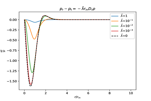
Figure 5.10: In this figure, we plot $\frac{\partial\tilde{\rho}}{\partial r}$ against $r/r_{\mathrm{m}}$ by considering positive values of $\tilde{\lambda}$. We have chosen $n=0$, $q=10^{-10}$ and $\epsilon_{0}=10^{-1}$.

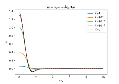
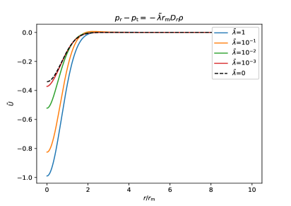
Figure 5.11: In the left panel we show $\tilde{\rho}$ against $r/r_{\mathrm{m}}$ for different values of $\tilde{\lambda}>0$ while in the right one we show $\tilde{U}$ against $r/r_{\mathrm{m}}$ for different values of $\tilde{\lambda}>0$. We have chosen $n=0$, $q=10^{-10}$ and $\epsilon_{0}=10^{-1}$.

5.6 Towards the PBH formation thershold

After specifying the initial conditions for the hydrodynamic and metric perturbations, the next step is to compute numerically the PBH formation threshold $\delta_{\mathrm{c}}$ as a function of the degree of the anisotropy. Given the fact that we have not yet fully completed the numerical computation of $\delta_{\mathrm{c}}$ (work in progress) we give below a synthetic overview about the prescription one should follow to make such computation.

1. Given the anisotropy parameters $\lambda$ or $\tilde{\lambda}$ and $n$ and the amplitude of the curvature profile $\mathcal{A}$, one can compute the characteristic scale of the collapsing overdensity region $r_{\mathrm{m}}$, corresponding to the location where the compaction function defined in Eq. (2.3) has a maximum. This is done on the superhorizon regime when the compaction function is time-independent. This allows to compute the averaged perturbation amplitude of the collapsing overdensity $\delta_{\mathrm{m}}$, defined as the integral of the energy density perturbation over a spherical volume of radius $r_{\mathrm{m}}$ in Eq. (2.8).

2. Then, one should evolve the non linear hydrodynamic equations and check if a black hole apparent horizon is formed, i.e. when the condition $R(r,t)=2M(r,t)$ is fulfilled. The threshold $\delta_{c}$ is obtained then as the limiting intermediate case between overcritical perturbations ($\delta_{\mathrm{m}}>\delta_{c}$) collapsing into a black hole, and subcritical ones ($\delta_{\mathrm{m}}<\delta_{c}$), where the perturbation bouncing back into the medium without forming a black hole. In practice this is computed with a bisection method up to a certain precision.

To estimate here what one would obtain performing numerical simulations of our anisotropic models, we compute $\delta_{\mathrm{c}}$ by adopting a perturbative approach based on the assumption that $\delta_{\mathrm{c}}$ depends on the shape of the initial energy density profile in the same way as it happens in the isotropic case. If so, one can compute the dependence of $\delta_{\mathrm{c}}$ in terms of the degree of anisotropy of the gravitational collapse, computing how the shape of the initial perturbation is changed by the amplitude of the anisotropy.

To find this dependence, we use the analytic relation for the threshold of PBH formation as a function of the shape parameter, $\alpha$, defined as

$$\alpha\equiv-\frac{r^{2}_{\mathrm{m}}\mathcal{C}^{\prime\prime}(r_{\mathrm{m}})}{4\mathcal{C}(r_{\mathrm{m}})}.$$ (5.115)

For our analytic estimation of $\delta_{\mathrm{c}}$, we use the numerical fit given by Eq. (44) of  [285] where the threshold for PBH formation is given as a polynomial function of $\alpha$ as follows,

$$\delta_{\mathrm{c}}=\begin{cases}\alpha^{0.047}-0.50\quad 0.1\lesssim\alpha\lesssim 7\\ \alpha^{0.035}-0.475\quad 7\lesssim\alpha\lesssim 13\\ \alpha^{0.026}-0.45\quad 13\lesssim\alpha\lesssim 30.\end{cases}$$ (5.116)

Fixing the amplitude of the anisotropy measured by $\lambda$ or $\tilde{\lambda}$ one should firstly compute $r_{\mathrm{m}}$ by requiring $\mathcal{C}(r_{\mathrm{m}})=0$ and subsequently compute at $r_{\mathrm{m}}$ the compaction function and its second derivative, which allows to compute the shape parameter, $\alpha$ using Eq. (5.115). By inserting then this into Eq. (5.116) one can compute the threshold for PBH formation. Below, we give the dependence of $\alpha$ and $\delta_{\mathrm{c}}$ in terms of $\lambda$ or $\tilde{\lambda}$ when $f(r,t)=R(r,t)$ or $f(r,t)=\rho^{n}(r,t)$. In particular, when $f(r,t)=\rho^{n}(r,t)$, we choose $n=0$ , $q=10^{-10}$ and $\epsilon_{0}=10^{-1}$. For our practical purposes, we fix as well the perturbation amplitude $\delta_{\mathrm{m}}=0.5$, a condition from which one can extract the amplitude $\mathcal{A}$ of the curvature profile for a fixed value of the amplitude of the anisotropy.

Figure 5.12: The shape parameter (left panel) and the PBH formation threshold (right panel) as a function of the degree of anisotropy $\lambda$. The blue circles stand for the prescription in which $p_{\mathrm{r}}-p_{\mathrm{t}}=-\tilde{\lambda}R(r,t)D_{\mathrm{r}}p_{\mathrm{r}}$ while the red ones correspond to the prescription in which $p_{\mathrm{r}}-p_{\mathrm{t}}=-\tilde{\lambda}R(r,t)D_{\mathrm{r}}\rho$.

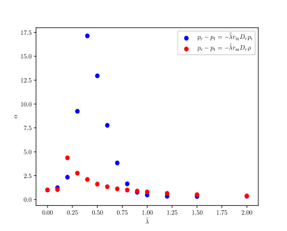
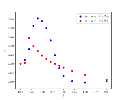
Figure 5.13: The shape parameter (left panel) and the PBH formation threshold (right panel) as a function of the degree of anisotropy $\tilde{\lambda}$. The blue circles stand for the prescription in which $p_{\mathrm{r}}-p_{\mathrm{t}}=-\tilde{\lambda}r_{\mathrm{m}}\left(\frac{\rho}{\rho_{\mathrm{b,inf}}}\right)^{n}D_{\mathrm{r}}p_{\mathrm{r}}$ while the red ones correspond to the prescription in which $p_{\mathrm{r}}-p_{\mathrm{t}}=-\tilde{\lambda}r_{\mathrm{m}}\left(\frac{\rho}{\rho_{\mathrm{b,inf}}}\right)^{n}D_{\mathrm{r}}\rho$. In both prescriptions we have chosen $n=0$, $q=10^{-10}$ and $\epsilon_{0}=10^{-1}$.

As one can see from the figures below, an initial increase of $\delta_{\mathrm{c}}$ is observed, which is somehow expected for an increasing amplitude of the anisotropy, as mentioned in the previous sections. This is because in this regime, the radial pressure is enhanced with respect to the tangential one, an effect that works against the gravitational collapse. On the contrary, after a critical value of $\lambda$ or $\tilde{\lambda}$, $\delta_{\mathrm{c}}$ follows a decreasing behavior, an effect that could not be predicted. However, if one makes a careful analysis on the dependence of $\alpha$ in terms of $\lambda$ or $\tilde{\lambda}$ it is possible to identify a dependence of $\alpha\propto(\lambda\mathrm{\;or\;}\tilde{\lambda})\left.\frac{\partial(\tilde{p}_{\mathrm{r}}\mathrm{\;or\;}\tilde{\rho})}{\partial r}\right|{r_{\mathrm{m}}}$, with two competing terms: $\lambda$ or $\tilde{\lambda}$, and $\left.\frac{\partial(\tilde{p}_{\mathrm{r}}\mathrm{\;or\;}\tilde{\rho})}{\partial r}\right|{r_{\mathrm{m}}}$ which decreases in absolute value with respect to $\lambda$ or $\tilde{\lambda}$ as it can be seen numerically from Figs. 5.1, 5.5, 5.7 and 5.10. Consequently, one expects a critical turning point in the behavior of $\delta_{\mathrm{c}}$. The explicit dependence of $\delta_{\mathrm{c}}$ in terms of $\lambda$ or $\tilde{\lambda}$ has not been deduced yet and it is part of an ongoing research work.

At this point, one should comment the fact that in the case where $f(r,r)=R(r,t)$ the behavior of $\alpha$ and $\delta_{\mathrm{c}}$ when the difference $p_{\mathrm{r}}-p_{\mathrm{t}}$ is modeled as proportional to pressure gradients is quite different with respect to the case when $p_{\mathrm{r}}-p_{\mathrm{t}}$ is modeled as proportional to energy density gradients. In the first case, $\delta_{\mathrm{c}}$ initially increases with $\lambda$ and then after a critical point decreases. However, in the second case, $\delta_{\mathrm{c}}$ initially decreases and then increases with $\lambda$. This behavior could be caused from the fact that the EoS for $f(r,t)=R(r,t)$ is given not only in terms of local quantities such as $p_{\mathrm{r}}$ and $\rho$ but also in terms of non local quantities as the areal radius $R(r,t)$. This is an indication that this model is not so well physically motivated. This claim however needs to be confirmed by performing full numerical simulations.

Finally, it is important to stress out that Eq. (5.116) gives just an estimation of $\delta_{\mathrm{c}}$ for values of $\lambda$ or $\tilde{\lambda}$ in which $p_{\mathrm{t}}-p_{\mathrm{t}}\ll 1$ and cannot be trusted if one wants to find the exact value of $\delta_{\mathrm{c}}$ in presence of anisotropies. For this reason it is important to perform in the future the full numerical analysis and evolve the non-linear hydrodynamic equations. Despite this fact, the results obtained here give a reasonable estimation of the effect of the anisotropy.

Chapter 6 Conclusions - Outlook

Since ’70s, when PBHs were initially introduced by Novikov and Zeldovich  [1] and Stephen Hawking  [8], they have been attracting an increasing attention within the scientific community. Already in  [2], PBHs were proposed to contribute to dark matter and seed the supermassive black holes we see in the center of galaxies  [5, 6]. In ’90s, the first formation scenarios made their appearance ranging from inflationary production mechanisms  [286, 287], primordial phase transitions  [288, 289] up to gravitational collapse of topological defects  [290, 291, 292]. In the following decades, a huge progress took place regarding the analytical  [108] and numerical  [107, 82, 90] methods describing the PBH gravitational collapse process. In addition, the wide range of masses of PBHs gave access to different physical phenomena, a fact which gave the possibility to make significant progress on the constraints of the abundance of PBHs at different mass ranges by studying data from different observational probes  [29].

In the view of this significant progress on the field of PBHs physics, both at the theoretical and the observational level, a first goal of this thesis was to constrain parameters of the early universe through PBH physics and vice-versa to constrain PBHs by studying aspects of the early universe. In particular, in a first part of the thesis we set constraints on parameters of the early universe, namely the energy scale at end of inflation and the energy scale at the onset of the radiation era, by studying PBHs produced from the preheating instability in the context of single-field inflationary models  [30, 31]. Interestingly, we find that PBHs can be so abundantly produced that reheating can proceed from their evaporation. By taking also into account the decay of the inflaton field to a radiation fluid, we show that the resonant instability structure of preheating responsible for the PBH production is not disrupted by the presence of the radiative products of the inflaton, a fact which points out to the presence of a generic PBH production mechanism from the preheating instability in the context of single-field inflation.

Regarding future prespectives of this first research part of this thesis, one should point out the possibility to narrow down the observational predictions of the CMB. Particularly, for a fixed single-field inflationary potential, the only theoretical uncertainty in the observational predictions of the CMB is on the number of e-folds elapsed between the time when the CMB pivot scale exits the Hubble radius and the end of inflation, namely $\Delta N_{*}$. This number depends on the energy scale at the end of inflation, $\rho_{\mathrm{inf}}$, which is given by the inflationary model under consideration, the energy density at the onset of the radiation era $\rho_{\mathrm{rad}}$, and the averaged equation-of-state parameter between the end of inflation and the onset of the radiation era, $\bar{w}_{\mathrm{rad}}$ and reads  [293]

$$\Delta N_{*} =\frac{1-3\bar{w}_{\mathrm{rad}}}{12(1+\bar{w}_{\mathrm{rad}})}\ln\left(\frac{\rho_{\mathrm{rad}}}{\rho_{\mathrm{inf}}}\right)+\frac{1}{4}\ln\left(\frac{\rho_{*}}{9M_{\scriptscriptstyle{\mathrm{Pl}}}^{4}}\frac{\rho_{*}}{\rho_{\mathrm{inf}}}\right)$$ (6.1)

$$-\ln\left(\frac{k_{\mathrm{P}}/a_{\mathrm{now}}}{\tilde{\rho}^{1/4}_{\mathrm{\gamma,now}}}\right),$$ (6.2)

where $\bar{w}_{\mathrm{rad}}\equiv\frac{\int_{N_{\mathrm{inf}}}^{N_{\mathrm{rad}}}w(N)dN}{\Delta N_{\mathrm{rad}}}$ is the mean equation of state during reheating with $\Delta N_{\mathrm{rad}}=N_{\mathrm{rad}}-N_{\mathrm{inf}}$ , $\rho_{*}$ is the energy scale at the time when the CMB pivot scale exits the Hubble radius, $a_{\mathrm{now}}$ is the present value of the scale factor, and $\tilde{\rho}_{\mathrm{\gamma,now}}$ is the the energy density of radiation today rescaled by the number of relativistic degrees of freedom. Taking the pivot scale $k_{\mathrm{P}}/a_{\mathrm{now}}$ to be 0.05Mpc^-1 and $\tilde{\rho}_{\mathrm{\gamma}}$ to its measured value, the last term is $N_{0}\equiv-\ln\left(\frac{k_{\mathrm{P}}/a_{\mathrm{now}}}{\tilde{\rho}^{1/4}_{\mathrm{\gamma,now}}}\right)\simeq 61.76$.

Considering then constraints on the energy scale at the end of inflation and on energy scale at the onset of the radiation from PBHs produced during preheating, one can constrain $\Delta N_{*}$. In particular, by using the theoretical setup introduced  [30] one can compute $\bar{w}_{\mathrm{rad}}$ and from Eq. (6.1) constrain $\Delta N_{*}$. In Fig. 6.1 we give the constraints on $\Delta N_{*}$ as a function of $\rho_{\mathrm{inf}}$ and $\rho_{\mathrm{rad}}$.

Figure 6.1: $\Delta N_{*}$ as a function of $\rho_{\mathrm{inf}}$ and $\rho_{\mathrm{rad}}$, when the PBH mass fraction is renormalised by inclusion (left panel) and by premature ending (right panel).

Vice-versa, in a second part of the thesis, we study a backreaction problem of the gravitational waves induced by energy density perturbations underlain by a gas of PBHs. In particular, by requiring that the induced gravitational waves associated to PBHs are not overproduced in an era when ultralight PBHs ($m_{\mathrm{PBH}}<10^{9}\mathrm{g}$) dominate the energy budget of the universe we set constraints on the abundance of PBHs at the time they form as a function of their mass  [32]. To the best of our knowledge, these constraints are actually the first solid model-independent constraints in the literature regarding ultralight PBHs, which are poorly constrained since they evaporate before BBN and they do not leave a direct observational imprint apart from rather speculative Planckian relics produced as leftovers of the PBH Hawking evaporation.

At this point, one should point out the potential detectability of the gravitational-wave signal of the stochastic background of induced gravitational waves produced from a universe filled with ultralight PBHs. As we found in  [32], the peak frequency of the relevant gravitational-wave spectrum, given in Eq. (6.3), depends crucially on the initial PBH abundance when the PBH forms, $\Omega_{\mathrm{PBH,f}}$, and the PBH mass, $m_{\mathrm{PBH}}$, and lies within the frequency band of future gravitational-wave experiments like the Einstein Telescope (ET) [294], the Laser Interferometer Space Antenna (LISA) [295, 256] and the Square Kilometre Array (SKA) facility [296],

$$\frac{f}{\mathrm{Hz}}\simeq\frac{1}{\left(1+z_{\mathrm{eq}}\right)^{1/4}}\left(\frac{H_{0}}{70\mathrm{kms^{-1}Mpc^{-1}}}\right)^{1/2}\left(\frac{g_{\mathrm{eff}}}{100}\right)^{1/6}\Omega^{2/3}_{\mathrm{PBH,f}}\left(\frac{m_{\mathrm{PBH}}}{10^{9}\mathrm{g}}\right)^{-5/6},$$ (6.3)

where $H_{0}$ is the value of the Hubble parameter today, $g_{\mathrm{eff}}$ is the effective number of relativistic degrees of freedom at PBH formation time and $z_{\mathrm{eq}}$ is the redshift at matter-radiation equality. See also the following Fig. 6.2 in which the peak frequency is plotted as a function of the initial PBH abundance at formation time and the PBH mass.

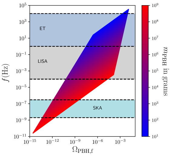
Figure 6.2: The peak frequency of the stochastic gravitational wave background induced by a dominating gas of primordial black holes, as a function of their abundance at the time they form, $\Omega_{\mathrm{PBH,f}}$ (horizontal axis), and their mass $m_{\mathrm{PBH}}$ (colour coding). The displayed region of parameter space corresponds to values of $m_{\mathrm{PBH}}$ and $\Omega_{\mathrm{PBH,f}}$ such that black holes dominate the universe content for a transient period, they form after inflation and Hawking evaporate before BBN and that the induced gravitational waves are not overproduced, see Eq. (4.34). In practice, Eq. (6.3) is displayed with $g_{\mathrm{eff}}=100$, $z_{\mathrm{eq}}=3387$ and $H_{0}=70\,\mathrm{km}\,\mathrm{s}^{-1}\,\mathrm{Mpc}^{-1}$. For comparison, the detection frequency bands of ET, LISA and SKA are also shown. Figure credited  [32].

This is very important, since one can potentially further constrain ultralight PBHs from the upcoming data of future gravitational-wave observational probes. However, in order to give an explicit answer on whether this signal can be detected, one should take into account the dynamical evolution of the gravitational-wave spectrum from the end of the PBH-dominated era up to our epoch by resolving the gradual transition from the PBH-dominated era up to the subsequent radiation-dominated era which is rather subtle  [297, 192].

Finally, in the last part of the thesis, which is a work in progress and not published yet, we study aspects of the gravitational collapse of a radiation fluid to PBHs in the presence of anisotropies. In particular, we model in a covariant way the difference between the radial, $p_{\mathrm{r}}$, and the tangential pressure, $p_{\mathrm{t}}$, as proportional to either to pressure or energy density gradients with a proportionality factor $\lambda$ which accounts for the anisotropic nature of the gravitational collapse. Then, by performing a gradient expansion approximation on superhorizon scales at the level of the Einstein’s equations we extract the initial conditions for the hydrodynamic and metric perturbations in the presence of anisotropies. At the end, we deduce the dependence of the PBH formation threshold in terms of the anisotropy parameter $\lambda$ adopting a perturbative approach based on the assumption that $\delta_{\mathrm{c}}$ depends on the shape of the initial energy density profile in the same way as in the isotropic case. Although this is something that requires a numerical investigation which is an ongoing work, the results obtained here give a reasonable estimation of what is the effect of the anisotropy.

The next step is to evolve in time the non-linear hydrodynamic equations and study numerically the PBH apparent horizon formation and the explicit dependence of the PBH formation threshold on the anisotropy parameter $\lambda$. In this way, we will be able to derive the dependence as well of the PBH mass fraction on the anisotropy parameter $\lambda$. In this way, one can make use of the observational constraints on the PBH abundances and set tight constraints on the anisotropy parameter of our model. In addition, in the case where the anisotropy parameter $\lambda$ becomes dimensionful, it depends on the intrinsic energy scale of the problem, which in our case is the energy scale when the perturbations are generated, namely the energy scale at the end of inflation. Consequently, in this regime one can translate the potential observational constraints on $\lambda$ to constraints on the energy scale at the end of inflation giving access in this way to the inflationary landscape.

To summarize, with this thesis we studied aspects of the early universe through PBH physics. In particular, we set constraints on cosmological parameters of the early universe by studying PBHs produced during the preheating instability in the context of single-field inflation and we constrained PBHs by studying induced gravitational waves produced in an early PBH-dominated era. In addition, we studied some facets of the PBH gravitational collapse in the presence of anisotropies. The research findings related to this thesis can potentially open up new directions in the field of PBH physics as stressed out above shedding light at the same time in the understanding of the physics of the early universe.

Chapitre 7 Compte Rendu Français

Ce compte rendu contient une description courte des résultats principaux de cette thèse sur articles.

7.1 Contexte Scientifique

Les trous noirs primordiaux (TNP), proposés initialement dans les années ’70  [1, 298, 299], attirent de plus en plus l’attention de la communauté scientifique, vu qu’ils peuvent adresser un grand nombre de problèmes de la cosmologie contemporaine. D’après des arguments récents, ils peuvent potentielllement constituer une partie ou la totalité de la matière noire en expliquant en même temps la génération des structures gravitationnels de grande échelle à travers les fluctuations Poissoniennes  [3, 4]. De plus, les TNP pourraient fournir les graines des trous noirs supemassifs au milieu des noyaux galactiques [198, 6] aussi bien que consituer les ancêtres des évenements de coalescence des trous noirs recemment détectés par les missions LIGO/VIRGO  [7] à travers l’émission des ondes gravitationnels.

Malgré le fait que les TNP ne sont pas encore détectés, ces objets astrophysiques jouent un rôle cardinal sur la cosmologie étant donné le fait que avec eux, dépendamment de leur masse, on peut explorer et contraindre une grande variété de phénomènes physiques. En particulier, les TNP de pétite masse ($m_{\mathrm{PBH}}\leq 10^{15}\mathrm{g}$) qui se sont évaporés maintenant peuvent donner accès à la physique de l’univers primordial comme la physique de l’inflation et des perturbations cosmologiques primordiales [17], la physique du rechauffement de l’univers et de la nucléosynthèse après le Big Bang (BBN) [18, 19] , la physique des ondes gravitationnels primordiaux  [21] et des transitions de phase primordiales  [22] aussi bien que la physique du fond cosmologique (Cosmic Microwave Background) [20]. De l’autre côté, avec les TNP d’une masse intérmediaire qui s’évaporent à notre époque cosmique, on peut investiguer des phénomènes de l’astrophysique de haute énérgie comme le fond des rayons cosmiques par le biais de l’évaporation Hawking de TNP [23]. Enfin, les TNP d’une grande masse qui existent encore aujourd’hui, i.e. ($m_{\mathrm{PBH}}>10^{15}\mathrm{g}$), peuvent donner accès à des phénomènes de la physique gravitationnelle, comme les lentilles gravitationnelles  [24, 25], à la formation des structures de grande échelle  [26] aussi bien que à la physique du secteur noir de l’univers, à savoir la matière noire  [27] et l’énergie noire [28].

7.2 Recherche effectuée pendant la thèse

Après avoir suscité avant le contexte scientifique sur le domaine de TNP on résume ici les résultats de la recherche effectuée pendant mes études doctorales, pendant laquelle on a combiné des aspects de l’univers primordial et de la physique des ondes gravitationnels avec la physique des TNP. On a étudié aussi des facettes du processus de l’effondrement gravitationnel des TNP en présence des anisotropies.

7.2.1 TNP de l’instabilité de préchauffement

L’inflation constitue la théorie cardinale de la cosmologie primordiale qui peut décrire d’une manière concordante les conditions initiales de l’univers primordial et résoudre les problèmes fondamentaux de l’époque du Hot Big Bang, à savoir les problème de l’horizon et de la platitude. De plus, l’inflation peut générer naturellement les petrurbations cosmologiques primordiales qui ont engendré les structures de grande échelle à l’univers aussi bien que le fond cosmologique.

Pour adrésser ainsi à tous ces aspects mentionnés avant, l’inflation postule une phase initiale pendant laquelle l’univers s’étend avec un rythme accéléré et son budget énergétique est dominé par un champ scalaire, $\phi$, rapporté comme l’inflaton, qui est associé à un potentiel inflationnaire $V(\phi)$. Après avoir passé d’une phase de roulement lent tout au long de son potentiel, l’infaton commence à osciller à l’origine de son potentiel, un comportement oscillatoire qui conduit inévitablement à l’émergence d’une structure d’instabilité résonante au niveau de l’équation de mouvement des perturbations scalaires. C’est alors pendant cette phase oscillatoire de l’inflaton, souvant citée comme préchauffement, qu’on étudie la production des TNP dans le contexte des modèles inflationnaires avec un champ scalaire  [30, 31].

En particulier, on a trouvé que les TNP produits pendant la période du prechauffement peuvent potentiellement dominer le contenu énergétique de l’univers et conduire au réchauffement de l’univers, pendant lequel les particules élémentaires du Modèle Standard se produisent, à travers leur évaporation. Par conséquent, en exigeant que les TNP ne dominent pas le budget énergétique de l’univers pendant la période de la nucléosynthèse après le Big Bang et qu’ils ne surproduisent pas des reliques Planckiennes, on a imposé des contraintes concernant l’échelle d’énergie de l’univers au commencement de l’époque du Hot Big Bang, $\rho_{\mathrm{rad}}$ aussi bien l’échelle d’énergie de l’univers à la fin de la période d’inflation, $\rho_{\mathrm{inf}}$  [30]. Dans la Fig. 7.1 ci-dessous on montre les contraintes combinées au niveau des paramètres $\rho_{\mathrm{rad}}$ et $\rho_{\mathrm{inf}}$ pour les deux prescriptions de renormalisation de la fonction de masse des TNP étant introduites pour adresser le problème de la surproduction de TNP. Pour plus de détails à voir sur  [30].

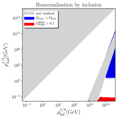
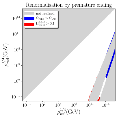
Figure 7.1: Contraintes combinées au niveau des paramètres $\rho_{\mathrm{rad}}$ et $\rho_{\mathrm{inf}}$ quand la fonction de masse de TNP se renormalise par inclusion (panneau gauche) et par l’arrêt prématuré de l’instabilité de préchauffement (panneau droit). Les régions grises sont exclues vu qu’elles correspondent aux valeurs de $\rho_{\mathrm{rad}}$, qui ne peuvent pas être réalisés naturellement tandis que les régions rouges sont aussi exclues parce qu’elles conduisent aux abondances très grandes de TNP à l’époque de BBN. Les régions bleues sont exclues vu que dans lequelles quelq’un se confronte avec une surpoduction des reliques Planckiennes. La région qui reste, démontrée en blanc, est celle qui est permise. Figure créditée à  [30].

Ensuite, vu que sur  [30] on a considéré que les auto-interactions de l’inflaton, on a avancé notre recherche en couplant d’une manière covariante le champ inflaton avec un fluide de radiation afin d’assurer la transition de la période de l’inflation à la période du Hot Big Bang. Enfin, on a trouvé que la desintégration de l’inflaton en radiation ne change pas la structure de l’instabilité résonante du préchauffement, responsable pour la production de TNP, jusqu’à le moment où le fluide de radiation domine énergétiquement l’univers. Par suite, l’émergence de l’instabilité de résonance qui favorise la formation des TNP est encore présente pendant la période du préchauffement, en indiquant de cette façon un mécanisme de production de TNP général dans le contexte des modèles inflationnaires avec un champ scalaire [31].

7.2.2 Ondes gravitationnelles d’un univers rempli des TNP

Au sein de cette thèse, on combiné aussi des aspects de la physique des ondes gravitationnelles avec la physique des TNP. Évidemment, il y a pleins de canaux connectant la physique des TNP avec la physique des ondes gravitationnnelles. Parmi eux, on peut mettre en exergue les trois plus significatifs. Tout d’abord, il faut se référer aux ondes gravitationnelles de second ordre qui se sont induites par les perturbations de courbure primordiales qui ont précédé et ont donné naissance aux TNP. Un second canal possible de connection de TNP avec les ondes gravitationnelles est le fond stochastique gravitationnel des gravitons émis par le biais de l’évaporation Hawking des TNP. Enfin, le troisième canal, le plus étudié par rapport aux autres, est le fond stochastique des ondes gravitationnelles produites à travers des événements de coalescence des TNP.

Pendant le temps de déroulement de cette thèse, on s’était concentré sur les ondes gravitationnellles induites par des perturbations scalaires associés aux TNP eux-mêmes, et pas aux perturbations de courbure primordiales qui ont donné naissance aux TNP. En particulier, on a étudié un gas des TNP qui crée son propre potentiel gravitationnel et qui induit inévitablement un fond des ondes gravitationnelles à travers des effets gravitationnels de seconde ordre. Plus spécifiquement, on a traité des régimes où les TNP constituent la composante principale du budget énergétique de l’univers pendant une période avant BBN. En demandant alors que ces ondes gravitationnelles induites ne se produisent pas en excès à la fin de la période de domination énergétique des TNP, on a imposé des contraintes indépedentes du modèle de production de TNP sur leur abondance au moment de leur formation en fonction de leur masse. Ci-dessous, on donne notre approximation analytique des contraintes extraites au niveau de l’abondance des TNP,

$$\Omega_{\mathrm{PBH,f}}<1.4\times 10^{-4}\left(\frac{10^{9}\mathrm{g}}{m_{\mathrm{PBH}}}\right)^{1/4},$$ (7.1)

où $\Omega_{\mathrm{PBH,f}}$ et $m_{\mathrm{PBH}}$ sont l’abondance initiale des TNP le moment de leur formation et la masse des TNP respectivement.

Vue que ces TNP se forment et s’évaporent avant BBN, leurs masses sont miniscules, à savoir $m_{\mathrm{PBH}}\in\left[10\mathrm{g},10^{9}\mathrm{g}\right]$ et d’après la bibliographie internationale sur le sujet, ils ne sont pas bien contraints. En étudiant alors les ondes gravitationnelles induites produites dans une époque de domination énergétique des TNP on a pu imposer les premières contraintes solides sur les TNP ultra-légers  [32]. On voit aussi ci-dessous dans la Fig. 7.2 les contraintes extraites au niveau de paramètres $\Omega_{\mathrm{PBH,f}}$ et $m_{\mathrm{PBH}}$.

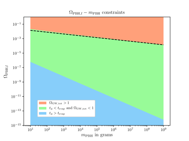
Figure 7.2: L’énergie de densité fractionnelle aux ondes gravitationnelles, $\Omega_{\mathrm{GW,tot}}$, au moment d’évaporation de TNP en fonction de deux paramètres, à savoir la masse des TNP, $m_{\mathrm{PBH}}$, et leur abondance, $\Omega_{\mathrm{PBH,f}}$, le moment ils se forment. La région orange correspond aux régimes où $\Omega_{\mathrm{GW}}(t_{\mathrm{evap}})>1$ et conduit à la surproducion des ondes gravitationnelles. Cette région est alors exclue. La région bleue correspond aux régimes où les TNP ne dominent jamais le budget énergétique de l’univers tandis que la région verte correspond aux cas où on se confronte avec des phases transitoires de domination des TNP et où les ondes gravitationnelles ne se produisent pas en excès. La ligne noire en tirés représente notre approximation analytique  (7.1), par rapport à la contrainte supérieure au niveau de $\Omega_{\mathrm{PBH,f}}$. Évidemment, on peut voir qu’il nous fournit avec une approximation très bonne de la frontière entre les régions orange et verte.

7.3 Effondrement anisotrope des TNP

Enfin, pendant cette thèse, on a abordé aussi une autre facette de la physique des TNP, réliée à l’effondrement gravitationnel en présence des anisotropies. En particulier, en adoptant la symétrie sphérique, on a introduit une pression anisotrope afin de tenir en compte le caractère anisotrope de l’éffondrement gravitationnel d’un fluide de radiation. Plus spécifiquement, étant inspiré par le comportement des objets ultra-compacts qui imitent le comportement dynamique des trous noirs, on modélé d’une façon covariante la difference entre la densité de la pression radiale, $p_{\mathrm{r}}$, et la densité de la pression tangentielle, $p_{\mathrm{t}}$, en postulant que la différence $p_{\mathrm{r}}-p_{\mathrm{t}}$ est proportionnelle soit aux gradients de pression soit aux gradients de densité d’énergie,

$$p_{\mathrm{t}} = p_{\mathrm{r}}+\lambda f(r,t)k^{\mu}\nabla_{\mu}p_{\mathrm{r}}\quad\textrm{(gradients de pression)}$$

or

$$p_{\mathrm{t}} = p_{\mathrm{r}}+\lambda f(r,t)k^{\mu}\nabla_{\mu}\rho\quad\ \textrm{(gradients de densité d'énergie)},$$ (7.3)

où $k^{\mu}$ est un quadrivecteur spatial unitaire orthogonal à la quadrivitesse du fluide, $\nabla_{\mu}$ correspond à la dérivative covariante, $\lambda$ est un paramètre qui correspond au degré de l’anisotropie et $f(r,t)$ est une fonction libre. Ensuite, en utilisant la méthode de l’éxpansion de gradients au niveau des équations hydrodynamiques, on a extrait les conditions initiales pour les perturbations hydrodynamiques et metriques en fonction du profile de courbure $K(r)$, rélié à la géométrie de l’éspace-temps.

Enfin, on a extrait la dépendence du seuil de formation de TNP, $\delta_{\mathrm{c}}$, en fonction du degré de l’anisotropie $\lambda$ en supposant que $\delta_{\mathrm{c}}$ dépend de la forme du profil initial de la densité d’énergie de la même manière que dans le cas isotrope. Malgré le fait que cela demande une exploration numérique, constituant un travail en cours, les resultats obtenus ici donnent une estimation raisonable de l’effet de l’anisotropie. Dans la figure ci-dessous, on voit la dépendence du $\delta_{\mathrm{c}}$ en fonction du degré de l’anisotropie $\lambda$ ou $\tilde{\lambda}$, dépendant de la modelisation de la différence $p_{\mathrm{r}}-p_{\mathrm{t}}$.

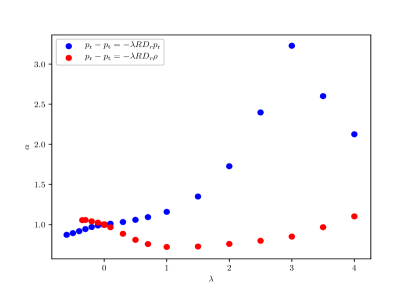
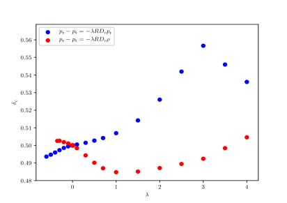
Figure 7.3: Le paramètre de forme (panneau gauche) et le seuil de formation de TNP (panneau droit) en fonction du degré de l’anisotropie $\tilde{\lambda}$. Les circles bleus correspondent à la modelisation où $p_{\mathrm{r}}-p_{\mathrm{t}}=-\tilde{\lambda}R(r,t)D_{\mathrm{r}}p_{\mathrm{r}}$ tandis que les circles rouges correspondent à la modelisation où $p_{\mathrm{r}}-p_{\mathrm{t}}=-\tilde{\lambda}R(r,t)D_{\mathrm{r}}\rho$.

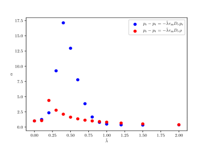
Figure 7.4: Le paramètre de forme (panneau gauche) et le seuil de formation de TNP (panneau droit) en fonction du degré de l’anisotropie $\tilde{\lambda}$. Les circles bleus correspondent à la modelisation où $p_{\mathrm{r}}-p_{\mathrm{t}}=-\tilde{\lambda}r_{\mathrm{m}}\left(\frac{\rho}{\rho_{\mathrm{b,inf}}}\right)^{n}D_{\mathrm{r}}p_{\mathrm{r}}$ tandis que les circles rouges correspondent à la modelisation où $p_{\mathrm{r}}-p_{\mathrm{t}}=-\tilde{\lambda}r_{\mathrm{m}}\left(\frac{\rho}{\rho_{\mathrm{b,inf}}}\right)^{n}D_{\mathrm{r}}\rho$. Dans les deux modélisations on a choisi $n=0$, $q=10^{-10}$ and $\epsilon_{0}=10^{-1}$.

7.4 Conclusions - Perspectives

Depuis les années ’70, quand les TNP s’étaient initialement introduits par Novikov and Zeldovich  [1] et Stephen Hawking  [8], ils attirent de plus en plus l’attention de la communauté scientifique. Déjà, dans  [2] les TNP sont proposés afin de contribuer au budget énergétique de la matière noire et engender les trous noirs supermassifs qu’on voit au centre des galaxies  [5, 6]. Dans les années ’90, les premiers mécanismes de production de TNP se sont apparus, se variant des modèles inflattionaires [286, 287] et des transitions de phase primordiales  [288, 289] jusqu’à l’effondrement gravitationnel des défauts topologiques  [290, 291, 292]. Dans les decennies suivantes, un grand progrès s’était manifesté par rapport aux méthodes analytiques  [108] et numériques  [107, 82, 90] décrivant le processus de l’effondrement gravitationnel des TNP. De plus, la grande gamme de masse des TNP nous a permis d’avoir accès aux phénomènes physiques différents donnant de cette façon la possibilité de contraindre l’abondance des TNP en étudiant les données observationnelles des différentes éxperiences  [29].

Vu ce progrès significatif au domaine de la physique des TNP, au niveau théorique et à la fois observationnel, un premier but de cette thèse était de poser des contraintes aux paramètres de l’univers primordial à travers la physique des TNP et vice-versa de contraindre les TNP en étudiant quelques aspects de l’univers primordial. En particulier, dans la première partie de la thèse, on a posé des contraintes sur des paramètres cosmologiques de l’univers primordial, à savoir l’échelle d’énergie à la fin de la période de l’inflation et l’échelle de l’énergie au commencement de l’époque du Hot Big Bang en étudiant des TNP se produisant pendant la période de préchauffement au contexte de la théorie de l’inflation avec un champ scalaire  [30, 31]. Il est intéressant de noter que les TNPs se produisant pendant la période de préchauffement se produisent si abondamment qu’ils peuvent conduire au réchauffement de l’univers par le biais de leur évaporation.

En ce qui concerne les perspectives futures de cette première partie de la thèse il faut souligner les contraintes potentielles que quelq’un peut poser sur les prévisions observationnelles du CMB. Plus spécifiquement, pour un potentiel inflattionaire avec un champ scalaire fixe, la seule incertitude au niveau des prévisions observationnelles du CMB se repose au nombre d’e-folds passés entre le temps dans lequel l’échelle pivot du CMB franchit le rayon Hubble et la fin de la période l’inflation, à savoir $\Delta N_{*}$. Ce nombre, dépendant de l’échelle d’énergie à la fin de la période de l’inflation, $\rho_{\mathrm{inf}}$, qui est donné par le modèle d’inflation sous considération, de l’échelle de l’énergie au commencement de l’époque du Hot Big Bang, $\rho_{\mathrm{rad}}$, et du paramètre de l’équation d’état moyen entre la fin de l’inflation et le commencement de l’époque du Hot Big Bang, $\bar{w}_{\mathrm{rad}}$, s’écrit comme  [293]

$$\Delta N_{*} =\frac{1-3\bar{w}_{\mathrm{rad}}}{12(1+\bar{w}_{\mathrm{rad}})}\ln\left(\frac{\rho_{\mathrm{rad}}}{\rho_{\mathrm{inf}}}\right)+\frac{1}{4}\ln\left(\frac{\rho_{*}}{9M_{\scriptscriptstyle{\mathrm{Pl}}}^{4}}\frac{\rho_{*}}{\rho_{\mathrm{inf}}}\right)$$ (7.4)

$$-\ln\left(\frac{k_{\mathrm{P}}/a_{\mathrm{now}}}{\tilde{\rho}^{1/4}_{\mathrm{\gamma,now}}}\right),$$ (7.5)

où $\bar{w}_{\mathrm{rad}}\equiv\frac{\int_{N_{\mathrm{inf}}}^{N_{\mathrm{rad}}}w(N)dN}{\Delta N_{\mathrm{rad}}}$ est le paramètre de l’équation d’état moyen pendant la période du réchauffement, $\Delta N_{\mathrm{rad}}=N_{\mathrm{rad}}-N_{\mathrm{inf}}$ , $\rho_{*}$ est l’échelle d’énergie au moment où l’échelle pivot du CMB franchit le rayon Hubble, $a_{\mathrm{now}}$ est le facteur d’échelle aujourd’hui et $\tilde{\rho}_{\mathrm{\gamma,now}}$ est la densité d’énergie de radiation aujourd’hui. En prenant alors l’échelle pivot du CMB $k_{\mathrm{P}}/a_{\mathrm{now}}$ égal à 0.05Mpc^-1 et $\tilde{\rho}_{\mathrm{\gamma}}$ à son valeur mesuré aujourd’hui, le dernier terme en Eq. (7.4) devient $N_{0}\equiv-\ln\left(\frac{k_{\mathrm{P}}/a_{\mathrm{now}}}{\tilde{\rho}^{1/4}_{\mathrm{\gamma,now}}}\right)\simeq 61.76$.

Par suite, en considérant les contraintes sur l’échelle d’énergie à la fin de la période de l’inflation et l’échelle de l’énergie au commencement de l’époque du Hot Big Bang en étudiant des TNP se produisant pendant la période de préchauffement, on peut contraindre la quantité $\Delta N_{*}$. En particulier, en utilisant le setup théorique developpé en  [30], quelq’un peut calculer $\bar{w}_{\mathrm{rad}}$ et de l’Eq. (7.4) poser des contraintes sur $\Delta N_{*}$. Dans la Fig. 7.5,on donne les contraintes au niveau de $\Delta N_{*}$ en fonction de $\rho_{\mathrm{inf}}$ et $\rho_{\mathrm{rad}}$.

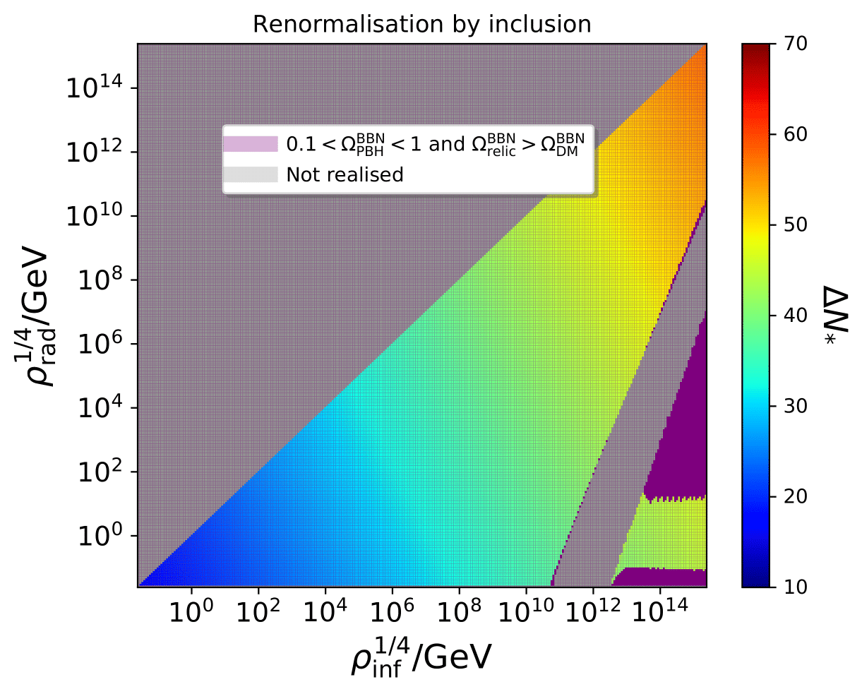
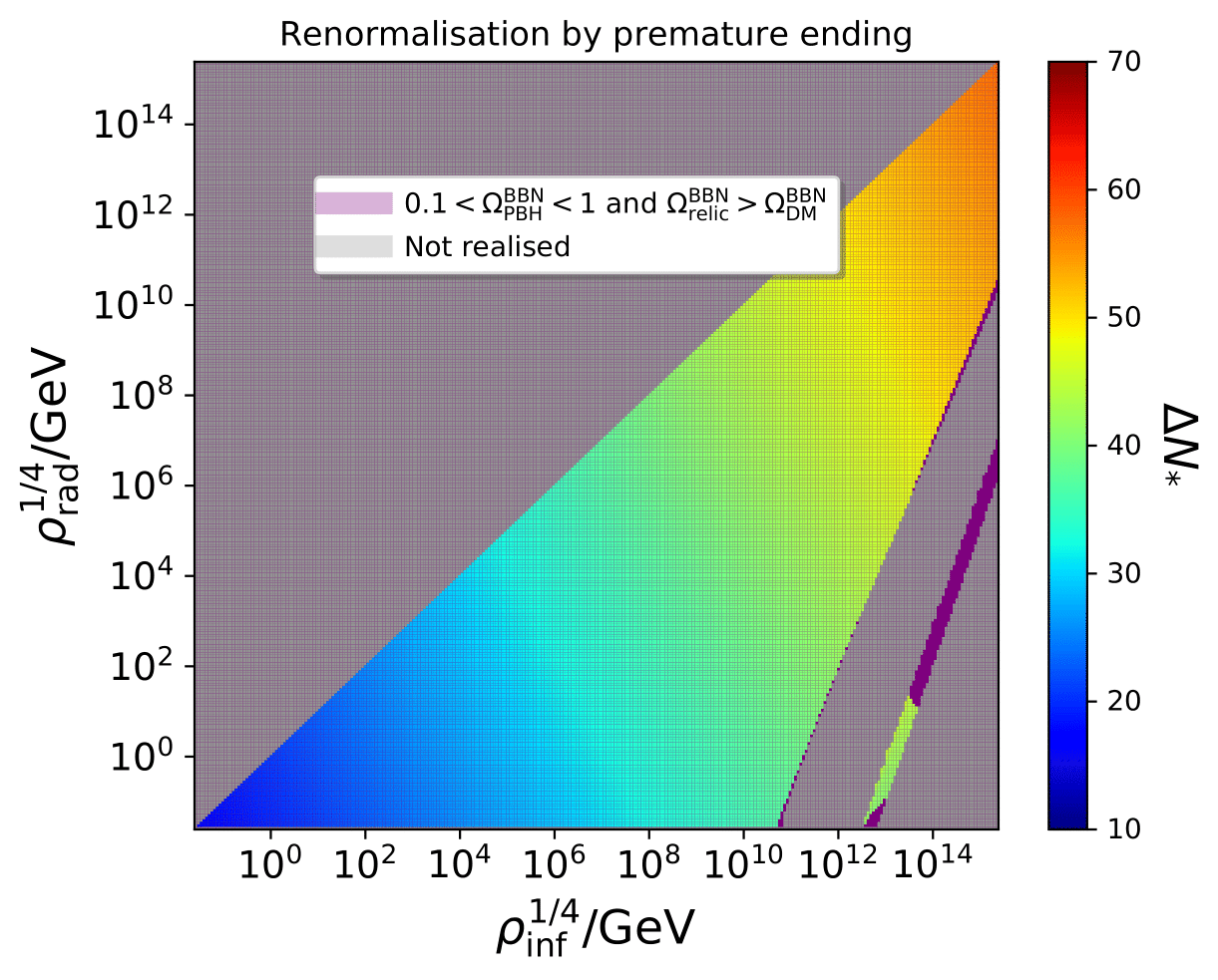
Figure 7.5: $\Delta N_{*}$ en fonction de $\rho_{\mathrm{inf}}$ et $\rho_{\mathrm{rad}}$, quand la fonction de masse des TNP est renormalisée avec le schéma de l’inclusion des TNP (panneau gauche) aussi bien qu’avec le shéma de l’arrêt premature de l’instabilité du préchauffement (panneau droit). Pour plus de détails à voir sur  [30].

Vice-versa, dans la seconde partie de la thèse, on a étudié un problème de réaction en retour des ondes gravitationnelles induites par des perturbations d’énergie de densité sous-tendues par un gaz des TNP. Plus spécifiquement, en demandant que les ondes gravitationnelles induites associées aux TNP ne se produisent pas en excès pendant une période cosmique où des TNP ultralégers ($m_{\mathrm{PBH}}<10^{9}\mathrm{g}$) dominent le budget énergétique de l’univers on a posé des contraintes sur l’abondance des TNP au moment où ils se forment en fonction de leur masse  [32]. Au meilleur de notre connaissance, elles se sont les premières contraintes solides indépendentes du modèle de production des TNP ultalégers dans la littérature internationale, étant donné le fait que les TNP ultralégers sont très pauvrement contraintes vu qu’ils s’évaporent avant BBN et ils ne laissent pas une empreinte observationnelle directe à part des reliques Planck spéculatives qui se produisent comme un vestige après l’évaporation Hawking des TNP.

Sur ce point, il faut mettre en exergue la détectabilité potentielle du signal stochastique des ondes gravitationnelles induites produites dans un univers étant dominé par des TNP ultralégers. De façon interessante, on a trouvé dans  [32] que la fréquence de crête du spectrum respective, donné par l’Eq. (6.3) dépend de manière décisive de l’abondance initiale des TNP au moment de leur formation, $\Omega_{\mathrm{PBH,f}}$, et de la masse du TNP, $m_{\mathrm{PBH}}$, et se trouve de la gamme de fréquences des expériences des ondes gravitationnelles comme l’Einstein Telescope (ET)  [294], le Laser Interferometer Space Antenna (LISA) [295, 256] et le Square Kilometre Array (SKA) [296],

$$\frac{f}{\mathrm{Hz}}\simeq\frac{1}{\left(1+z_{\mathrm{eq}}\right)^{1/4}}\left(\frac{H_{0}}{70\mathrm{kms^{-1}Mpc^{-1}}}\right)^{1/2}\left(\frac{g_{\mathrm{eff}}}{100}\right)^{1/6}\Omega^{2/3}_{\mathrm{PBH,f}}\left(\frac{m_{\mathrm{PBH}}}{10^{9}\mathrm{g}}\right)^{-5/6},$$ (7.6)

où $H_{0}$ est le valeur du paramètre Hubble aujourd’hui, $g_{\mathrm{eff}}$ est le nombre effective des degrés de liberté relativistes au moment de fomation des TNP et $z_{\mathrm{eq}}$ est le décalage vers le rouge au moment de l’équilibre énergétique entre la matière et la radiation. À voir aussi la Fig. 7.6 dans laquelle la fréquence de crête se montre en fonction de $\Omega_{\mathrm{PBH,f}}$ et de $m_{\mathrm{PBH}}$.

Figure 7.6: La fréquence de crête du fond stochastique des ondes gravitationnelles induites par un gaz des TNP dominant le budget énergétique de l’univers, en fonction de l’abondance des TNP au moment où ils se forment, $\Omega_{\mathrm{PBH,f}}$ (axe horizontal), et de leur masse, $m_{\mathrm{PBH}}$ (code des couleurs). La région de l’éspace des paramètres démontrée correspond aux valeurs de $m_{\mathrm{PBH}}$ et de $\Omega_{\mathrm{PBH,f}}$ tels que les TNP dominent le budget énergétique de l’univers pendant une période transitoire, se forment après la fin de la période de l’inflation et s’évaporent avant BBN et que les ondes gravitationnelles induites ne se produisent pas en excès, à voir Eq. (7.1). En pratique, Eq. (6.3) est démontrée avec $g_{\mathrm{eff}}=100$, $z_{\mathrm{eq}}=3387$ et $H_{0}=70\,\mathrm{km}\,\mathrm{s}^{-1}\,\mathrm{Mpc}^{-1}$. Pour comparaison, les bandes des fréquences détectables par ET, LISA et SKA sont aussi montrées. Figure creditée à  [32].

Cette perspective est très importante vu que quelq’un peut potentiellement contraindre plus les TNP ultralégers en étudiant les donnés qui vont arriver par les expériences observationnelles futures des ondes gravitationnelles. Par contre, afin de donner une réponse finale si ce signal stochastique des ondes gravitationnelles induites associées aux TNP ultralégers peut être détecté ou non, il faut tenir en compte l’évolution dynamique du spectrum des ondes gravitationnelles de la fin de l’époque de domination des TNP jusq’à notre époque. Et pour cela, il est nécessaire de résoudre la transition graduelle de l’époque cosmique dominée par des TNP à l’époque cosmique successive dominée par la radiation, une étude assez subtile  [297, 192].

Enfin, dans la dernière partie de la thèse, qui est un travail en cours pas encore publié, on étudie des aspects de l’effondrement gravitationnel d’un fluide radiative aux TNP en présence des anisotropies. En particulier, on modèle d’une manière covariante la différence entre la pression radiale, $p_{\mathrm{r}}$, et la pression tangentielle, $p_{\mathrm{t}}$, en postulant que la différence $p_{\mathrm{r}}-p_{\mathrm{t}}$ est proportionnelle soit aux gradients de pression soit aux gradients de densité d’énergie avec un paramètre de proportionalité $\lambda$ qui est équivelent à un paramètre d’anisotropie. En réalisant alors le programme perturbative de l’expansion des gradients au niveau des équations d’Einstein on déduit les conditions initiales des perturbations hydrodynamiques et metriques en présence des anisotropies. De plus, on déduit la dépendence du seuil de formation de TNP, $\delta_{\mathrm{c}}$, en fonction de $\lambda$ en supposant que $\delta_{\mathrm{c}}$ dépend de la même manière que dans le cas isotrope de la forme du profil initial de densité d’énergie.

Le prochain pas à faire est d’évoluer les équations hydrodynamiques non-linéaires et étudier numériquement la formation de l’horizon du TNP et la dépendence explicite du seuil de formation des TNP avec le degré de l’anisotropie $\lambda$. Par conséquent, on pourra calculer le seuil de formation des TNP en présence des anisotropies et dériver aussi la dépendence de la fonction de masse des TNP avec le paramètre $\lambda$. Et cela va ouvrir des perspectives sur notre recherehce vu qu’en utilisant les contraintes des abondances des TNP quelq’un peut contraindre le degré de l’anisotropie $\lambda$ de notre modèle. De plus, dans le cas où le paramètre $\lambda$ a des dimensions, il se dépend lui-même de l’échelle d’énergie intrinsèque du processus de l’effondrement gravitationnel, qui est dans notre cas l’échelle d’énergie au moment où les perturbations sont générées, à savoir l’échelle d’énergie à la fin de la période de l’inflation. Par conséquent, quelq’un peut traduire les contraintes observationnelles potentielles au niveau du degré de l’anisotropie $\lambda$ aux contraintes au niveu de l’échelle d’énergie à la fin de la période de l’inflation donnant accès de cette façon au panorama inflationnaire.

Pour résumer, avec cette thèse on a étudié des aspects de l’univers primordial par le biais de la physique des TNP. Plus particulièrement, on a posé des contraintes sur des paramètres cosmologiques de l’univers primordial en étudiant les TNP se produisant pendant la période du préchauffement au contexte de la théorie de l’inflation avec un champ scalaire. De plus, en étudiant aussi les ondes gravitationnelles induites produites dans une époque cosmique où des TNP constituent la composante dominante du budget énergétique de l’univers, on a posé des contraintes indépendentes du modèle de production des TNP sur l’abondance des TNP au moment où ils se forment en fonction de leur masse. De surcroît, on a étudié des facettes de l’effondrement gravitationnel des TNP en présence des anisottropies. Comme il était mis en évidence avant, les résultats de la recherche effectuée au sein de cette thèse peuvent potentiellement ouvrir des directions nouvelles sur le domaine de la physique des TNP et porter un éclairage sur la compréhension de la physique de l’univers primordial.

Appendix A Appendix

A.1 The sound speed in a time-dependent $w$ background

Here, we extract the sound speed of a general adiabatic fluid, $c^{2}_{\mathrm{s}}$, with a time-dependent equation-of-state parameter, $w$. In a general system, the pressure density $p$ is a function of the energy density $\rho$ as well as of the entropy density $S$, i.e. $p=p(\rho,S)$. Consequently, one can write the following equation

$$\delta p=c^{2}_{\mathrm{s}}\delta\rho+\left(\frac{\partial p}{\partial S}\right)_{\mathrm{\rho}}\delta S,$$ (A.1)

where the sound speed $c^{2}_{\mathrm{s}}$ is defined as $c^{2}_{\mathrm{s}}\equiv\left(\frac{\partial p}{\partial\rho}\right)_{\mathrm{S}}$. If one considers then an adiabatic system then they should require that $\left(\frac{\partial p}{\partial S}\right)_{\mathrm{\rho}}=0$, i.e. there is no entropy production. Consequently, for such a system $c^{2}_{\mathrm{s}}$ becomes

$$c^{2}_{\mathrm{s}}=\frac{\delta p}{\delta\rho},$$ (A.2)

Given then the fact that the background pressure and energy densities of an adiabatic fluid system, $p$ and $\rho$ depend only on time, one can rewrite Eq. (A.2) by introducing the derivation with respect to the conformal time and using the chain rule, as

$$c^{2}_{\mathrm{s}}=\frac{p^{\prime}}{\rho^{\prime}},$$ (A.3)

where the prime denotes differentiation with respect to the conformal time, $\eta$. Using therefore the continuity equation (1.18) written with the conformal time as the time variable as well as time differentiating the equation of state for a time dependent equation-of-state parameter $w$, one can straightforwardly obtain that

$$c^{2}_{\mathrm{s}}(\eta)=w(\eta)-\frac{1}{3\left[1+w(\eta)\right]\mathcal{H}(\eta)}\frac{\mathrm{d}w}{\mathrm{d}\eta},$$ (A.4)

where $\mathcal{H}\equiv\frac{a^{\prime}}{a}$ is the conformal Hubble parameter.

A.2 The External Derivative

Below we derive the relation $D_{\mathrm{k}}f=D_{\mathrm{r}}f+D_{\mathrm{t}}f$ as well Eq. (5.12) by making use of the external derivative which is defined to be the unique $R$-linear mapping from $k$-forms to $(k+1)$-forms satisfying the following properties  [300]:

1. $\mathrm{d}f$ is the differential of $0$-forms (smooth functions) f.

2. $\mathrm{d}(\mathrm{d}f)=0$ for every $k$-form $f$.

3. $\mathrm{d}(a\wedge b)=\mathrm{d}a\wedge b+(-1)^{p}a\wedge\mathrm{d}b$, where $b$ is a $p$-form.

Having that into our mind, we can prove here the relation $D_{\mathrm{k}}f=D_{\mathrm{r}}f+D_{\mathrm{t}}f$ for a general function $f$. If we multiply (5.10) with a function f ($0$-form) and take the external derivative we have that

$$G\mathrm{d}f\wedge\mathrm{d}u+f\mathrm{d}G\wedge\mathrm{d}u=A\mathrm{d}f\wedge\mathrm{d}t+f\mathrm{d}A\wedge\mathrm{d}t-B\mathrm{d}f\wedge\mathrm{d}r-f\mathrm{d}B\wedge\mathrm{d}r\Leftrightarrow$$

$$G\mathrm{d}f\wedge\mathrm{d}u=A\mathrm{d}f\wedge\mathrm{d}t-B\mathrm{d}f\wedge\mathrm{d}r\Leftrightarrow$$

$$G\left(\frac{\partial f}{\partial r}\right)_{\mathrm{u}}\mathrm{d}r\wedge\mathrm{d}u=A\left(\frac{\partial f}{\partial r}\right)_{\mathrm{t}}\mathrm{d}r\wedge\mathrm{d}t+B\left(\frac{\partial f}{\partial t}\right)_{\mathrm{r}}\mathrm{d}r\wedge\mathrm{d}t\Leftrightarrow$$

$$G\left(\frac{\partial f}{\partial r}\right)_{\mathrm{u}}\mathrm{d}r\wedge\mathrm{d}u=A\frac{G}{A}\left(\frac{\partial f}{\partial r}\right)_{\mathrm{t}}\mathrm{d}r\wedge\mathrm{d}u+B\frac{G}{A}\left(\frac{\partial f}{\partial t}\right)_{\mathrm{r}}\mathrm{d}r\wedge\mathrm{d}u\Leftrightarrow$$

$$D_{\mathrm{k}}f=D_{\mathrm{r}}f+D_{\mathrm{t}}f,$$

where from the first to the second equality, we used the fact that the external derivative applied to (5.10) gives $\mathrm{d}G\wedge\mathrm{d}u=\mathrm{d}A\wedge\mathrm{d}t-\mathrm{d}B\wedge\mathrm{d}r$ and from the third to the forth equality we expressed $\mathrm{d}t$ in terms of $\mathrm{d}u$ and $\mathrm{d}r$ through (5.10).

Regarding now the derivation of Eq. (5.12), one obtains from (5.10) by applying the external derivative that

$$\mathrm{d}G\wedge\mathrm{d}u=\mathrm{d}A\wedge\mathrm{d}t-\mathrm{d}B\wedge\mathrm{d}r\Leftrightarrow$$

$$\left(\frac{\partial G}{\partial r}\right)_{\mathrm{u}}\mathrm{d}r\wedge\mathrm{d}u=\left(\frac{\partial A}{\partial r}\right)_{\mathrm{t}}\mathrm{d}r\wedge\mathrm{d}t+\left(\frac{\partial B}{\partial t}\right)_{\mathrm{r}}\mathrm{d}r\wedge\mathrm{d}t\Leftrightarrow$$

$$\left(\frac{\partial G}{\partial r}\right)_{\mathrm{u}}\mathrm{d}r\wedge\mathrm{d}u=\frac{G}{A}\left(\frac{\partial A}{\partial r}\right)_{\mathrm{t}}\mathrm{d}r\wedge\mathrm{d}u+\frac{G}{A}\left(\frac{\partial B}{\partial t}\right)_{\mathrm{r}}\mathrm{d}r\wedge\mathrm{d}u\Leftrightarrow$$

$$\frac{D_{\mathrm{k}}G}{G}=\frac{D_{\mathrm{r}}A}{A}+\frac{D_{\mathrm{t}}B}{B}\Leftrightarrow$$

$$\frac{D_{\mathrm{k}}G}{G}=\frac{D_{\mathrm{r}}A}{A}+\frac{D_{\mathrm{r}}U}{\Gamma}$$

where in the last equality we replace $\mathrm{t}$ from (5.10) and we used the fact that from $01$ Einstein equation, $\frac{D_{\mathrm{t}}B}{B}=\frac{D_{\mathrm{r}}U}{\Gamma}$.

A.3 Lower limit on the anisotropic parameter $\lambda/\tilde{\lambda}$

As we checked numerically for values of $\lambda<0$ less than a critical value the pressure and energy density gradient profiles were diverging at zero for both of the cases $f(r,t)=R(r,t)$ and $f(r,t)=\rho^{n}(r,t)$. This divergence can be explained by developing the pressure/energy density gradient profile around zero. We will work here with the energy density gradients. The same arguments apply also for the pressure gradients.

Starting with the case of $f(r,t)=R(r,t)$ and working with the differential equation 5.98 regarding the energy density gradients, one can develop $g(r)$ around zero as

$$g(r)=g_{0}+g_{1}r+g_{2}r^{2}/2,$$

where

$$g_{0}=g(0)=\tilde{\rho}^{\prime}(0)\,,\quad g_{1}=g^{\prime}(0)\quad\textrm{and}\quad g_{2}=g^{\prime\prime}(0)$$

Then, after a straightforward calculation, we get that

$$\frac{2\lambda r}{3}\left(1-\frac{\mathcal{A}r^{2}}{2}\right)\left(g_{1}+g_{2}r\right)+\left[\frac{8\lambda}{3}\left(1-\frac{\mathcal{A}r^{2}}{2}\right)+1\right]\left(g_{0}+g_{1}r+\frac{g_{2}r^{2}}{2}\right)-\tilde{\rho}^{\prime}_{\mathrm{iso}}\left(1-\frac{\mathcal{A}r^{2}}{2}\right)=0$$

Considering now only the $O(r^{0})$ terms we have that

$$g_{0}=\tilde{\rho}^{\prime}(0)=\lim_{r\to 0}\frac{\tilde{\rho}^{\prime}_{\mathrm{iso}}(r)}{1+\frac{8\lambda}{3}},$$

where $\rho^{\prime}_{\mathrm{iso}}=\frac{2}{3}\left\{\frac{\left[r^{3}K(r)\right]^{\prime}}{3r^{2}}\right\}^{\prime}r^{2}_{\mathrm{m}}$

If $\lambda<-3/8$ and since $\tilde{\rho}^{\prime}_{\mathrm{iso}}(0)=0^{-}$ one gets that $\tilde{\rho}^{\prime}(0)=0^{+}$ which is not consistent since $\tilde{\rho}^{\prime}(0)$ should approach zero from negative values. If however $\lambda>-3/8$ then one obtains the consistent result that $\tilde{\rho}^{\prime}(0)=0^{-}$. For the critical value $\lambda=-3/8$ then one has that

$$\tilde{\rho}^{\prime}(0)=\lim_{r\to 0}\frac{\tilde{\rho}^{\prime}_{\mathrm{iso}}(r)}{1+\frac{8\lambda}{3}}=\frac{0}{0}=\frac{\tilde{\rho}^{\prime\prime}_{\mathrm{iso}}(0)}{0}=-\infty\neq 0^{-},$$

after applying the De l’Hopital theorem and considering the fact that $\tilde{\rho}^{\prime\prime}_{\mathrm{iso}}(0)<0$.

Consequently, in the case of $p_{\mathrm{r}}-p_{\mathrm{t}}=-\lambda RD_{\mathrm{r}}\rho$ with $\lambda<0$ one gets that $\lambda$ should be larger than a critical value, namely $\lambda>\lambda_{\mathrm{c}}=-3/8$. In the case of $\lambda>0$ we do not have this problem since the expression $1+\frac{8\lambda}{3}$ is always positive, making thus $\tilde{\rho}^{\prime}(0)=0^{-}$ always for $\lambda>0$. As one may notice, $\lambda=\lambda_{\mathrm{c}}=-3/8$ is the value which makes zero the prefactor in front of $g(r)$ in Eq. (5.98) and which determines the sign of $\tilde{\rho}^{\prime}(0)$ at order $O(r^{0})$.

In the case of $p_{\mathrm{r}}-p_{\mathrm{t}}=-\lambda RD_{\mathrm{r}}p_{\mathrm{r}}$, following the same procedure one can conclude that $\lambda>\lambda_{\mathrm{c}}=-9/14$ in order not to confront divergent pressure gradient profiles at $r=0$.

Regarding now the case of $f(r,t)=\rho^{n}(r,t)$ one can apply the same gradient expansion around zero for the differential equation governing the pressure gradient profile’s behavior, i.e. Eq. (5.82) and derive the necessary condition for which the pressure gradient does not diverge at $r=0$. At this point, we should point out that given that in the formulation where $f(r,t)=\rho^{n}(r,t)$ we have more than one anisotropy parameters, the divergence condition should be given in terms of $\tilde{\lambda}$, $n$, $q$ and $\epsilon_{0}$.

Writing then $h(r)$ as

$$h(r)=h_{0}+h_{1}r+h_{2}r^{2}/2,$$

where

$$h_{0}=h(0)=\tilde{p_{\mathrm{r}}}^{\prime}(0)\,,\quad h_{1}=h^{\prime}(0)\quad\textrm{and}\quad h_{2}=h^{\prime\prime}(0)$$

and applying the same procedure as before one gets that

$$h_{0}=\tilde{p_{\mathrm{r}}}^{\prime}(0)=\lim_{r\to 0}\frac{\tilde{p}^{\prime}_{\mathrm{r,iso}}(r)}{\frac{2}{9(1-2n)}\frac{\tilde{\lambda}}{q}\left(\frac{q}{\epsilon_{0}}\right)^{3}\left[(5-6n)\left(\frac{q}{\epsilon_{0}}\right)^{4n-2}-2\right]},$$

where $\tilde{p}^{\prime}_{\mathrm{r,iso}}=\frac{2}{3}\left\{\frac{\left[r^{3}K(r)\right]^{\prime}}{3r^{2}}\right\}^{\prime}r^{2}_{\mathrm{m}}$. Consequently, the necessary condition in order not obtain a divergence at $r=0$ is

$$\frac{2}{9(1-2n)}\frac{\tilde{\lambda}}{q}\left(\frac{q}{\epsilon_{0}}\right)^{3}\left[(5-6n)\left(\frac{q}{\epsilon_{0}}\right)^{4n-2}-2\right]>0.$$ (A.5)

From the above expression if one fixes $q$ and $\epsilon_{0}$, one may identify two regimes, namely when $n>1/2$ and when $n<1/2$. In particular when $n>1/2$ given the fact that $q/\epsilon_{0}\ll 1$ one obtains that the second term in the brackets in Eq. (A.5) is the dominant one and that $\tilde{\lambda}$ should be positive, i.e. $\tilde{\lambda}>0$. If one the other hand $n<1/2$ the first term in the brackets is the dominant one and one can see straightforwardly that again $\tilde{\lambda}$ should be positive. Therefore, if $q/\epsilon_{0}\ll 1$ which is in general the case, $\tilde{\lambda}>\tilde{\lambda}_{\mathrm{c}}=0$.

In the case now where the difference between the radial and the tangential pressure is modeled as proportional to energy density gradients, following the same procedure as before and make a gradient expansion around $r=0$ at the level of 5.110 one gets the following necessary condition to avoid divergences around $r=0$.

$$\frac{3}{1-2n}\frac{\tilde{\lambda}}{q}\left(\frac{q}{\epsilon_{0}}\right)^{3}\left[1-\left(\frac{q}{\epsilon_{0}}\right)^{4n-2}\right]<0.$$ (A.6)

From the above equation, one can easily check that given the fact that $q/\epsilon_{0}\ll 1$, $\tilde{\lambda}$ should always be positive for any value of $n$, i.e. $\tilde{\lambda}>\tilde{\lambda}_{\mathrm{c}}=0$.

A.4 The limits $n\to 1/2$ and $n\to 1/4$ of $\Phi_{p_{\mathrm{r}}}$, $\Phi_{\rho}$, $I_{1,p_{\mathrm{r}}}$, $I_{2,p_{\mathrm{r}}}$, $I_{1,\rho}$ and $I_{2,\rho}$

Below we give the limits $n\to 1/2$ and $n\to 1/4$ of $\Phi_{p_{\mathrm{r}}}$, $\Phi_{\rho}$, $I_{1,p_{\mathrm{r}}}$,$I_{2,p_{\mathrm{r}}}$, $I_{1,\rho}$, $I_{2,\rho}$ which are given respectively by equations (5.70), (5.107), (5.80), (5.108) and (5.109).

$$\lim_{n\rightarrow 1/2}\Phi_{p_{\mathrm{r}}}(a) =-\frac{2\lambda\mathchoice{{\hbox{$\displaystyle\sqrt{\rho_{\mathrm{b,inf}}\,}$}\lower 0.4pt\hbox{\vrule height=4.30554pt,depth=-3.44446pt}}}{{\hbox{$\textstyle\sqrt{\rho_{\mathrm{b,inf}}\,}$}\lower 0.4pt\hbox{\vrule height=4.30554pt,depth=-3.44446pt}}}{{\hbox{$\scriptstyle\sqrt{\rho_{\mathrm{b,inf}}\,}$}\lower 0.4pt\hbox{\vrule height=3.01389pt,depth=-2.41113pt}}}{{\hbox{$\scriptscriptstyle\sqrt{\rho_{\mathrm{b,inf}}\,}$}\lower 0.4pt\hbox{\vrule height=2.15277pt,depth=-1.72223pt}}}}{a_{\mathrm{inf}}r_{\mathrm{m}}}\left(\frac{a}{a_{\mathrm{inf}}}\right)^{-3}\ln\left(\frac{a}{a_{\mathrm{inf}}}\right)$$ (A.7)

$$\lim_{n\rightarrow 1/2}I_{1,p_{\mathrm{r}}}(a) =\frac{\lambda\mathchoice{{\hbox{$\displaystyle\sqrt{\rho_{\mathrm{b,inf}}\,}$}\lower 0.4pt\hbox{\vrule height=4.30554pt,depth=-3.44446pt}}}{{\hbox{$\textstyle\sqrt{\rho_{\mathrm{b,inf}}\,}$}\lower 0.4pt\hbox{\vrule height=4.30554pt,depth=-3.44446pt}}}{{\hbox{$\scriptstyle\sqrt{\rho_{\mathrm{b,inf}}\,}$}\lower 0.4pt\hbox{\vrule height=3.01389pt,depth=-2.41113pt}}}{{\hbox{$\scriptscriptstyle\sqrt{\rho_{\mathrm{b,inf}}\,}$}\lower 0.4pt\hbox{\vrule height=2.15277pt,depth=-1.72223pt}}}}{2a_{\mathrm{inf}}r_{\mathrm{m}}}\left(\frac{a}{a_{\mathrm{inf}}}\right)^{-3}\left[2-2\frac{a}{a_{\mathrm{inf}}}+\ln\left(\frac{a}{a_{\mathrm{inf}}}\right)\right]$$ (A.8)

$$\lim_{n\rightarrow 1/4}I_{1,p_{\mathrm{r}}}(a) =-\frac{\lambda\rho^{1/4}_{\mathrm{b,ini}}}{2a_{\mathrm{inf}}r_{\mathrm{m}}}\left(\frac{a}{a_{\mathrm{inf}}}\right)^{-3}\left\{1+\frac{a}{a_{\mathrm{inf}}}\left[2\ln\left(\frac{a}{a_{\mathrm{inf}}}\right)-1\right]\right\}$$ (A.9)

$$\lim_{n\rightarrow 1/2}I_{2,p_{\mathrm{r}}}(a) =\frac{\lambda\mathchoice{{\hbox{$\displaystyle\sqrt{\rho_{\mathrm{b,inf}}\,}$}\lower 0.4pt\hbox{\vrule height=4.30554pt,depth=-3.44446pt}}}{{\hbox{$\textstyle\sqrt{\rho_{\mathrm{b,inf}}\,}$}\lower 0.4pt\hbox{\vrule height=4.30554pt,depth=-3.44446pt}}}{{\hbox{$\scriptstyle\sqrt{\rho_{\mathrm{b,inf}}\,}$}\lower 0.4pt\hbox{\vrule height=3.01389pt,depth=-2.41113pt}}}{{\hbox{$\scriptscriptstyle\sqrt{\rho_{\mathrm{b,inf}}\,}$}\lower 0.4pt\hbox{\vrule height=2.15277pt,depth=-1.72223pt}}}}{a_{\mathrm{inf}}r_{\mathrm{m}}}\left(\frac{a}{a_{\mathrm{inf}}}\right)^{-3}\left[\ln\left(\frac{a}{a_{\mathrm{inf}}}\right)-\frac{a}{a_{\mathrm{inf}}}+1\right]$$ (A.10)

$$\lim_{n\rightarrow 1/4}I_{2,p_{\mathrm{r}}}(a) =-\frac{\lambda\rho^{1/4}_{\mathrm{b,inf}}}{a_{\mathrm{inf}}r_{\mathrm{m}}}\left(\frac{a}{a_{\mathrm{inf}}}\right)^{-3}\left\{1+\left[\ln\left(\frac{a}{a_{\mathrm{inf}}}\right)-1\right]\frac{a}{a_{\mathrm{inf}}}\right\}$$ (A.11)

$$\lim_{n\rightarrow 1/2}\Phi_{\rho}(a) =-\frac{6\lambda\mathchoice{{\hbox{$\displaystyle\sqrt{\rho_{\mathrm{b,inf}}\,}$}\lower 0.4pt\hbox{\vrule height=4.30554pt,depth=-3.44446pt}}}{{\hbox{$\textstyle\sqrt{\rho_{\mathrm{b,inf}}\,}$}\lower 0.4pt\hbox{\vrule height=4.30554pt,depth=-3.44446pt}}}{{\hbox{$\scriptstyle\sqrt{\rho_{\mathrm{b,inf}}\,}$}\lower 0.4pt\hbox{\vrule height=3.01389pt,depth=-2.41113pt}}}{{\hbox{$\scriptscriptstyle\sqrt{\rho_{\mathrm{b,inf}}\,}$}\lower 0.4pt\hbox{\vrule height=2.15277pt,depth=-1.72223pt}}}}{a_{\mathrm{inf}}r_{\mathrm{m}}}\left(\frac{a}{a_{\mathrm{inf}}}\right)^{-3}\ln\left(\frac{a}{a_{\mathrm{inf}}}\right)$$ (A.12)

$$\lim_{n\rightarrow 1/2}I_{1,\rho}(a) =\frac{3\lambda\mathchoice{{\hbox{$\displaystyle\sqrt{\rho_{\mathrm{b,inf}}\,}$}\lower 0.4pt\hbox{\vrule height=4.30554pt,depth=-3.44446pt}}}{{\hbox{$\textstyle\sqrt{\rho_{\mathrm{b,inf}}\,}$}\lower 0.4pt\hbox{\vrule height=4.30554pt,depth=-3.44446pt}}}{{\hbox{$\scriptstyle\sqrt{\rho_{\mathrm{b,inf}}\,}$}\lower 0.4pt\hbox{\vrule height=3.01389pt,depth=-2.41113pt}}}{{\hbox{$\scriptscriptstyle\sqrt{\rho_{\mathrm{b,inf}}\,}$}\lower 0.4pt\hbox{\vrule height=2.15277pt,depth=-1.72223pt}}}}{2a_{\mathrm{inf}}r_{\mathrm{m}}}\left(\frac{a}{a_{\mathrm{inf}}}\right)^{-3}\left[2-2\frac{a}{a_{\mathrm{inf}}}+\ln\left(\frac{a}{a_{\mathrm{inf}}}\right)\right]$$ (A.13)

$$\lim_{n\rightarrow 1/2}I_{1,\rho}(a) =-\frac{3\lambda\rho^{1/4}_{\mathrm{b,inf}}}{2a_{\mathrm{inf}}r_{\mathrm{m}}}\left(\frac{a}{a_{\mathrm{inf}}}\right)^{-3}\left\{1+\frac{a}{a_{\mathrm{inf}}}\left[2\ln\left(\frac{a}{a_{\mathrm{inf}}}\right)-1\right]\right\}$$ (A.14)

$$\lim_{n\rightarrow 1/2}I_{2,\rho}(a) =\frac{3\lambda\mathchoice{{\hbox{$\displaystyle\sqrt{\rho_{\mathrm{b,inf}}\,}$}\lower 0.4pt\hbox{\vrule height=4.30554pt,depth=-3.44446pt}}}{{\hbox{$\textstyle\sqrt{\rho_{\mathrm{b,inf}}\,}$}\lower 0.4pt\hbox{\vrule height=4.30554pt,depth=-3.44446pt}}}{{\hbox{$\scriptstyle\sqrt{\rho_{\mathrm{b,inf}}\,}$}\lower 0.4pt\hbox{\vrule height=3.01389pt,depth=-2.41113pt}}}{{\hbox{$\scriptscriptstyle\sqrt{\rho_{\mathrm{b,inf}}\,}$}\lower 0.4pt\hbox{\vrule height=2.15277pt,depth=-1.72223pt}}}}{a_{\mathrm{inf}}r_{\mathrm{m}}}\left(\frac{a}{a_{\mathrm{inf}}}\right)^{-3}\left[\ln\left(\frac{a}{a_{\mathrm{inf}}}\right)-\frac{a}{a_{\mathrm{inf}}}+1\right]$$ (A.15)

$$\lim_{n\rightarrow 1/4}I_{2,\rho}(a) =-\frac{3\lambda\rho^{1/4}_{\mathrm{b,inf}}}{a_{\mathrm{inf}}r_{\mathrm{m}}}\left(\frac{a}{a_{\mathrm{inf}}}\right)^{-3}\left\{1+\left[\ln\left(\frac{a}{a_{\mathrm{inf}}}\right)-1\right]\frac{a}{a_{\mathrm{inf}}}\right\}.$$ (A.16)

References

- [1] Y. B. Zel’dovich and I. D. Novikov, The Hypothesis of Cores Retarded during Expansion and the Hot Cosmological Model, Soviet Astronomy 10 (Feb., 1967) 602.
- [2] G. F. Chapline, Cosmological effects of primordial black holes, Nature 253 (1975) 251–252.
- [3] P. Meszaros, Primeval black holes and galaxy formation, Astron. Astrophys. 38 (1975) 5–13.
- [4] N. Afshordi, P. McDonald and D. Spergel, Primordial black holes as dark matter: The Power spectrum and evaporation of early structures, Astrophys. J. Lett. 594 (2003) L71–L74, [astro-ph/0302035].
- [5] B. J. Carr and M. J. Rees, How large were the first pregalactic objects?, Monthly Notices of the Royal Astronomical Society 206 (Jan., 1984) 315–325.
- [6] R. Bean and J. Magueijo, Could supermassive black holes be quintessential primordial black holes?, Phys. Rev. D 66 (2002) 063505, [astro-ph/0204486].
- [7] LIGO Scientific, Virgo collaboration, B. Abbott et al., GWTC-1: A Gravitational-Wave Transient Catalog of Compact Binary Mergers Observed by LIGO and Virgo during the First and Second Observing Runs, Phys. Rev. X 9 (2019) 031040, [1811.12907].
- [8] S. Hawking, Gravitationally collapsed objects of very low mass, Monthly Notices of Royal Astronomic Society 152 (Jan., 1971) 75.
- [9] B. J. Carr and S. W. Hawking, Black holes in the early Universe, Monthly Notices of Royal Astronomic Society 168 (Aug., 1974) 399–416.
- [10] B. J. Carr, The Primordial black hole mass spectrum, Astrophys. J. 201 (1975) 1–19.
- [11] J. Rhoades, Clifford E. and R. Ruffini, Maximum mass of a neutron star, Phys. Rev. Lett. 32 (1974) 324–327.
- [12] J. L. Bernal, A. Raccanelli, L. Verde and J. Silk, Signatures of primordial black holes as seeds of supermassive black holes, JCAP 05 (2018) 017, [1712.01311].
- [13] H. Poulter, Y. Ali-Haïmoud, J. Hamann, M. White and A. G. Williams, CMB constraints on ultra-light primordial black holes with extended mass distributions, 1907.06485.
- [14] B. J. Carr, Primordial black holes: Do they exist and are they useful?, in 59th Yamada Conference on Inflating Horizon of Particle Astrophysics and Cosmology, 11, 2005. astro-ph/0511743.
- [15] S. Hawking, Particle Creation by Black Holes, Commun. Math. Phys. 43 (1975) 199–220.
- [16] S. Hawking, Black hole explosions, Nature 248 (1974) 30–31.
- [17] A. Kalaja, N. Bellomo, N. Bartolo, D. Bertacca, S. Matarrese, I. Musco et al., From Primordial Black Holes Abundance to Primordial Curvature Power Spectrum (and back), JCAP 10 (2019) 031, [1908.03596].
- [18] C. Sivaram and K. Arun, Big Bang Nucleosynthesis and Primordial Black Holes, arXiv e-prints (June, 2010) arXiv:1006.5342, [1006.5342].
- [19] C. Keith, D. Hooper, N. Blinov and S. D. McDermott, Constraints on Primordial Black Holes From Big Bang Nucleosynthesis Revisited, 2006.03608.
- [20] Y. Ali-Haïmoud and M. Kamionkowski, Cosmic microwave background limits on accreting primordial black holes, Phys. Rev. D 95 (2017) 043534, [1612.05644].
- [21] S. Clesse, J. García-Bellido and S. Orani, Detecting the Stochastic Gravitational Wave Background from Primordial Black Hole Formation, 1812.11011.
- [22] K. Jedamzik and J. C. Niemeyer, Primordial black hole formation during first order phase transitions, Phys. Rev. D 59 (1999) 124014, [astro-ph/9901293].
- [23] B. Carr, K. Kohri, Y. Sendouda and J. Yokoyama, Constraints on primordial black holes from the Galactic gamma-ray background, Phys. Rev. D 94 (2016) 044029, [1604.05349].
- [24] H. Niikura, M. Takada, S. Yokoyama, T. Sumi and S. Masaki, Constraints on Earth-mass primordial black holes from OGLE 5-year microlensing events, Phys. Rev. D 99 (2019) 083503, [1901.07120].
- [25] M. Zumalacarregui and U. Seljak, Limits on stellar-mass compact objects as dark matter from gravitational lensing of type Ia supernovae, Phys. Rev. Lett. 121 (2018) 141101, [1712.02240].
- [26] B. Carr and J. Silk, Primordial Black Holes as Generators of Cosmic Structures, Mon. Not. Roy. Astron. Soc. 478 (2018) 3756–3775, [1801.00672].
- [27] B. Carr and F. Kuhnel, Primordial Black Holes as Dark Matter: Recent Developments, 2006.02838.
- [28] S. Nesseris, D. Sapone and S. Sypsas, Evaporating primordial black holes as varying dark energy, Phys. Dark Univ. 27 (2020) 100413, [1907.05608].
- [29] B. Carr, K. Kohri, Y. Sendouda and J. Yokoyama, Constraints on Primordial Black Holes, 2002.12778.
- [30] J. Martin, T. Papanikolaou and V. Vennin, Primordial black holes from the preheating instability, 1907.04236.
- [31] J. Martin, T. Papanikolaou, L. Pinol and V. Vennin, Metric preheating and radiative decay in single-field inflation, JCAP 05 (2020) 003, [2002.01820].
- [32] T. Papanikolaou, V. Vennin and D. Langlois, Gravitational waves from a universe filled with primordial black holes, 2010.11573.
- [33] Planck collaboration, N. Aghanim et al., Planck 2018 results. VI. Cosmological parameters, 1807.06209.
- [34] A. G. Riess et al., A 2.4% Determination of the Local Value of the Hubble Constant, Astrophys. J. 826 (2016) 56, [1604.01424].
- [35] E. Di Valentino et al., Cosmology Intertwined II: The Hubble Constant Tension, 2008.11284.
- [36] A. Friedmann, On the Possibility of a world with constant negative curvature of space, Z. Phys. 21 (1924) 326–332.
- [37] G. Lemaitre, A Homogeneous Universe of Constant Mass and Growing Radius Accounting for the Radial Velocity of Extragalactic Nebulae, Gen. Rel. Grav. 45 (2013) 1635–1646.
- [38] H. Robertson, Kinematics and World-Structure, Astrophys. J. 82 (1935) 284–301.
- [39] A. G. Walker, On the formal comparison of Milne’s kinematical system with the systems of general relativity, Monthly Notices of the Royal Astronomical Society 95 (Jan., 1935) 263–269.
- [40] A. Einstein, The Field Equations of Gravitation, Sitzungsber. Preuss. Akad. Wiss. Berlin (Math. Phys. ) 1915 (1915) 844–847.
- [41] A. Einstein, The Foundation of the General Theory of Relativity, Annalen Phys. 49 (1916) 769–822.
- [42] D. Hilbert, Die Grundlagen der Physik. 1., Gott. Nachr. 27 (1915) 395–407.
- [43] A. Friedman, On the Curvature of space, Z. Phys. 10 (1922) 377–386.
- [44] A. Raychaudhuri, Relativistic cosmology. 1., Phys. Rev. 98 (1955) 1123–1126.
- [45] V. Faraoni, G. F. R. Ellis, J. T. Firouzjaee, A. Helou and I. Musco, Foliation dependence of black hole apparent horizons in spherical symmetry, Phys. Rev. D 95 (2017) 024008, [1610.05822].
- [46] E. W. Kolb and M. S. Turner, The Early Universe, vol. 69. 1990.
- [47] A. A. Starobinsky, A New Type of Isotropic Cosmological Models Without Singularity, Phys. Lett. B91 (1980) 99–102.
- [48] A. H. Guth, The Inflationary Universe: A Possible Solution to the Horizon and Flatness Problems, Phys.Rev. D23 (1981) 347–356.
- [49] A. D. Linde, A New Inflationary Universe Scenario: A Possible Solution of the Horizon, Flatness, Homogeneity, Isotropy and Primordial Monopole Problems, Phys.Lett. B108 (1982) 389–393.
- [50] A. Albrecht and P. J. Steinhardt, Cosmology for Grand Unified Theories with Radiatively Induced Symmetry Breaking, Phys.Rev.Lett. 48 (1982) 1220–1223.
- [51] A. D. Linde, Chaotic Inflation, Phys.Lett. B129 (1983) 177–181.
- [52] M. S. Turner, Coherent Scalar Field Oscillations in an Expanding Universe, Phys. Rev. D 28 (1983) 1243.
- [53] Y. Shtanov, J. H. Traschen and R. H. Brandenberger, Universe reheating after inflation, Phys. Rev. D 51 (1995) 5438–5455, [hep-ph/9407247].
- [54] L. Kofman, A. D. Linde and A. A. Starobinsky, Reheating after inflation, Phys. Rev. Lett. 73 (1994) 3195–3198, [hep-th/9405187].
- [55] L. Kofman, A. D. Linde and A. A. Starobinsky, Towards the theory of reheating after inflation, Phys. Rev. D 56 (1997) 3258–3295, [hep-ph/9704452].
- [56] D. Kirzhnits and A. D. Linde, Macroscopic Consequences of the Weinberg Model, Phys. Lett. B 42 (1972) 471–474.
- [57] S. Weinberg, Gauge and Global Symmetries at High Temperature, Phys. Rev. D 9 (1974) 3357–3378.
- [58] M. Dine, R. G. Leigh, P. Y. Huet, A. D. Linde and D. A. Linde, Towards the theory of the electroweak phase transition, Phys. Rev. D 46 (1992) 550–571, [hep-ph/9203203].
- [59] A. Sakharov, Violation of CP Invariance, C asymmetry, and baryon asymmetry of the universe, Sov. Phys. Usp. 34 (1991) 392–393.
- [60] G. R. Farrar and M. Shaposhnikov, Baryon asymmetry of the universe in the standard electroweak theory, Phys. Rev. D 50 (1994) 774, [hep-ph/9305275].
- [61] K. A. Olive, The Thermodynamics of the Quark - Hadron Phase Transition in the Early Universe, Nucl. Phys. B 190 (1981) 483–503.
- [62] G. Fuller, G. Mathews and C. Alcock, The Quark - Hadron Phase Transition in the Early Universe: Isothermal Baryon Number Fluctuations and Primordial Nucleosynthesis, Phys. Rev. D 37 (1988) 1380.
- [63] B.-l. Cheng and A. V. Olinto, Primordial magnetic fields generated in the quark - hadron transition, Phys. Rev. D 50 (1994) 2421–2424.
- [64] R. Alpher, H. Bethe and G. Gamow, The origin of chemical elements, Phys. Rev. 73 (1948) 803–804.
- [65] R. V. Wagoner, W. A. Fowler and F. Hoyle, On the Synthesis of elements at very high temperatures, Astrophys. J. 148 (1967) 3–49.
- [66] S. Sarkar, Big bang nucleosynthesis and physics beyond the standard model, Rept. Prog. Phys. 59 (1996) 1493–1610, [hep-ph/9602260].
- [67] P. Peebles, Recombination of the Primeval Plasma, Astrophys. J. 153 (1968) 1.
- [68] A. A. Penzias and R. W. Wilson, A Measurement of excess antenna temperature at 4080-Mc/s, Astrophys. J. 142 (1965) 419–421.
- [69] J. E. Gunn and I. Gott, J. Richard, On the Infall of Matter into Clusters of Galaxies and Some Effects on Their Evolution, Astrophys. J. 176 (1972) 1–19.
- [70] J. E. Gunn and B. A. Peterson, On the Density of Neutral Hydrogen in Intergalactic Space, Astrophys. J. 142 (1965) 1633.
- [71] SDSS collaboration, R. H. Becker et al., Evidence for Reionization at Z ~ 6: Detection of a Gunn-Peterson trough in a Z = 6.28 Quasar, Astron. J. 122 (2001) 2850, [astro-ph/0108097].
- [72] R. Barkana and A. Loeb, In the beginning: The First sources of light and the reionization of the Universe, Phys. Rept. 349 (2001) 125–238, [astro-ph/0010468].
- [73] E. T. Vishniac, Reionization and small-scale fluctuations in the microwave background, Astrophys. J. 322 (1987) 597–604.
- [74] Supernova Cosmology Project collaboration, S. Perlmutter et al., Measurements of and from 42 high redshift supernovae, Astrophys. J. 517 (1999) 565–586, [astro-ph/9812133].
- [75] Supernova Search Team collaboration, A. G. Riess et al., Observational evidence from supernovae for an accelerating universe and a cosmological constant, Astron. J. 116 (1998) 1009–1038, [astro-ph/9805201].
- [76] Supernova Search Team collaboration, B. P. Schmidt et al., The High Z supernova search: Measuring cosmic deceleration and global curvature of the universe using type Ia supernovae, Astrophys. J. 507 (1998) 46–63, [astro-ph/9805200].
- [77] W. Rindler, Visual horizons in world-models, Gen. Rel. Grav. 34 (2002) 133–153.
- [78] C. W. Misner, The Isotropy of the universe, Astrophys. J. 151 (1968) 431–457.
- [79] R. Dicke, Gravitation and the universe: The Jayne Lectures for 1969, Philadelphia: American Philosophical Institute (Jan., 1970) 61–62.
- [80] S. Hawking and W. Israel, General Relativity: An Einstein Centenary Survey. Univ. Pr., Cambridge, UK, 1979.
- [81] L. Canetti, M. Drewes and M. Shaposhnikov, Matter and Antimatter in the Universe, New J. Phys. 14 (2012) 095012, [1204.4186].
- [82] J. C. Niemeyer and K. Jedamzik, Near-critical gravitational collapse and the initial mass function of primordial black holes, Phys. Rev. Lett. 80 (1998) 5481–5484, [astro-ph/9709072].
- [83] I. Musco, J. C. Miller and A. G. Polnarev, Primordial black hole formation in the radiative era: Investigation of the critical nature of the collapse, Class. Quant. Grav. 26 (2009) 235001, [0811.1452].
- [84] I. Musco and J. C. Miller, Primordial black hole formation in the early universe: critical behaviour and self-similarity, Class. Quant. Grav. 30 (2013) 145009, [1201.2379].
- [85] M. W. Choptuik, Universality and scaling in gravitational collapse of a massless scalar field, Phys. Rev. Lett. 70 (1993) 9–12.
- [86] C. R. Evans and J. S. Coleman, Observation of critical phenomena and selfsimilarity in the gravitational collapse of radiation fluid, Phys. Rev. Lett. 72 (1994) 1782–1785, [gr-qc/9402041].
- [87] C. Gundlach, Critical phenomena in gravitational collapse, Living Rev. Rel. 2 (1999) 4, [gr-qc/0001046].
- [88] I. Hawke and J. Stewart, The dynamics of primordial black hole formation, Class. Quant. Grav. 19 (2002) 3687–3707.
- [89] I. Musco, Threshold for primordial black holes: Dependence on the shape of the cosmological perturbations, Phys. Rev. D 100 (2019) 123524, [1809.02127].
- [90] M. Shibata and M. Sasaki, Black hole formation in the friedmann universe: Formulation and computation in numerical relativity, Physical Review D 60 (Sep, 1999) .
- [91] W. H. Press and P. Schechter, Formation of galaxies and clusters of galaxies by selfsimilar gravitational condensation, Astrophys. J. 187 (1974) 425–438.
- [92] K. Jedamzik, The Cloud in cloud problem in the Press-Schechter formalism of hierarchical structure formation, Astrophys. J. 448 (1995) 1–17, [astro-ph/9408080].
- [93] J. Peacock and A. Heavens, Alternatives to the Press-Schechter cosmological mass function, Mon. Not. Roy. Astron. Soc. 243 (1990) 133–143.
- [94] R. G. Bower, The Evolution of groups of galaxies in the Press-Schechter formalism, Mon. Not. Roy. Astron. Soc. 248 (1991) 332.
- [95] J. Bond, S. Cole, G. Efstathiou and N. Kaiser, Excursion set mass functions for hierarchical Gaussian fluctuations, Astrophys. J. 379 (1991) 440.
- [96] M. Maggiore and A. Riotto, The Halo Mass Function from Excursion Set Theory. I. Gaussian fluctuations with non-Markovian dependence on the smoothing scale, Astrophys. J. 711 (2010) 907–927, [0903.1249].
- [97] M. Maggiore and A. Riotto, The Halo mass function from excursion set theory. II. The diffusing barrier, Astrophys. J. 717 (2010) 515–525, [0903.1250].
- [98] M. Maggiore and A. Riotto, The Halo mass function from excursion set theory. III. Non-Gaussian fluctuations, Astrophys. J. 717 (2010) 526–541, [0903.1251].
- [99] W. J. Percival, The build-up of halos within press-schechter theory, Mon. Not. Roy. Astron. Soc. 327 (2001) 1313, [astro-ph/0107437].
- [100] S. Matarrese, L. Verde and R. Jimenez, The Abundance of high-redshift objects as a probe of non-Gaussian initial conditions, Astrophys. J. 541 (2000) 10, [astro-ph/0001366].
- [101] M. LoVerde, A. Miller, S. Shandera and L. Verde, Effects of Scale-Dependent Non-Gaussianity on Cosmological Structures, JCAP 04 (2008) 014, [0711.4126].
- [102] I. E. Achitouv and P. S. Corasaniti, Non-Gaussian Halo Mass Function and Non-Spherical Halo Collapse: Theory vs. Simulations, JCAP 02 (2012) 002, [1109.3196].
- [103] I. E. Achitouv and P. S. Corasaniti, Primordial Bispectrum and Trispectrum Contributions to the Non-Gaussian Excursion Set Halo Mass Function with Diffusive Drifting Barrier, Phys. Rev. D 86 (2012) 083011, [1207.4796].
- [104] J. M. Bardeen, J. Bond, N. Kaiser and A. Szalay, The Statistics of Peaks of Gaussian Random Fields, Astrophys. J. 304 (1986) 15–61.
- [105] D. K. Nadezhin, I. D. Novikov and A. G. Polnarev, The hydrodynamics of primordial black hole formation, Soviet Astronomy 22 (Apr., 1978) 129–138.
- [106] G. V. Bicknell and R. N. Henriksen, Formation of primordial black holes., Astrophysics Journal 232 (Sept., 1979) 670–682.
- [107] I. D. Novikov and A. G. Polnarev, The Hydrodynamics of Primordial Black Hole Formation - Dependence on the Equation of State, Soviet Astronomy 24 (Apr., 1980) 147–151.
- [108] T. Harada, C.-M. Yoo and K. Kohri, Threshold of primordial black hole formation, Physical Review D 88 (Oct, 2013) .
- [109] A. Escrivà, C. Germani and R. K. Sheth, Universal threshold for primordial black hole formation, Phys. Rev. D 101 (2020) 044022, [1907.13311].
- [110] T. Nakama, T. Harada, A. Polnarev and J. Yokoyama, Identifying the most crucial parameters of the initial curvature profile for primordial black hole formation, JCAP 01 (2014) 037, [1310.3007].
- [111] M. Kawasaki and H. Nakatsuka, Effect of nonlinearity between density and curvature perturbations on the primordial black hole formation, Phys. Rev. D 99 (2019) 123501, [1903.02994].
- [112] S. Young, I. Musco and C. T. Byrnes, Primordial black hole formation and abundance: contribution from the non-linear relation between the density and curvature perturbation, JCAP 11 (2019) 012, [1904.00984].
- [113] C. Germani and R. K. Sheth, Nonlinear statistics of primordial black holes from Gaussian curvature perturbations, Phys. Rev. D 101 (2020) 063520, [1912.07072].
- [114] S. Young and M. Musso, Application of peaks theory to the abundance of primordial black holes, JCAP 11 (2020) 022, [2001.06469].
- [115] S. Young and C. T. Byrnes, Primordial black holes in non-Gaussian regimes, JCAP 1308 (2013) 052, [1307.4995].
- [116] S. Young, D. Regan and C. T. Byrnes, Influence of large local and non-local bispectra on primordial black hole abundance, JCAP 1602 (2016) 029, [1512.07224].
- [117] G. Franciolini, A. Kehagias, S. Matarrese and A. Riotto, Primordial Black Holes from Inflation and non-Gaussianity, JCAP 03 (2018) 016, [1801.09415].
- [118] V. De Luca, G. Franciolini, A. Kehagias, M. Peloso, A. Riotto and C. Ünal, The Ineludible non-Gaussianity of the Primordial Black Hole Abundance, JCAP 07 (2019) 048, [1904.00970].
- [119] C.-M. Yoo, J.-O. Gong and S. Yokoyama, Abundance of primordial black holes with local non-Gaussianity in peak theory, JCAP 09 (2019) 033, [1906.06790].
- [120] S. Young, C. T. Byrnes and M. Sasaki, Calculating the mass fraction of primordial black holes, JCAP 1407 (2014) 045, [1405.7023].
- [121] C. Germani and I. Musco, Abundance of Primordial Black Holes Depends on the Shape of the Inflationary Power Spectrum, Phys. Rev. Lett. 122 (2019) 141302, [1805.04087].
- [122] C.-M. Yoo, T. Harada, J. Garriga and K. Kohri, Primordial black hole abundance from random Gaussian curvature perturbations and a local density threshold, PTEP 2018 (2018) 123E01, [1805.03946].
- [123] C.-M. Yoo, T. Harada, S. Hirano and K. Kohri, Abundance of Primordial Black Holes in Peak Theory for an Arbitrary Power Spectrum, 2008.02425.
- [124] F. Kühnel and M. Sandstad, Ellipsoidal collapse and primordial black hole formation, Phys. Rev. D 94 (2016) 063514, [1602.04815].
- [125] C.-M. Yoo, T. Harada and H. Okawa, Threshold of Primordial Black Hole Formation in Nonspherical Collapse, Phys. Rev. D 102 (2020) 043526, [2004.01042].
- [126] M. He and T. Suyama, Formation threshold of rotating primordial black holes, Phys. Rev. D 100 (2019) 063520, [1906.10987].
- [127] V. De Luca, V. Desjacques, G. Franciolini, A. Malhotra and A. Riotto, The initial spin probability distribution of primordial black holes, JCAP 05 (2019) 018, [1903.01179].
- [128] T. W. Baumgarte and C. Gundlach, Critical collapse of rotating radiation fluids, Phys. Rev. Lett. 116 (2016) 221103, [1603.04373].
- [129] C. Gundlach and T. W. Baumgarte, Critical gravitational collapse with angular momentum II: soft equations of state, Phys. Rev. D 97 (2018) 064006, [1712.05741].
- [130] C. W. Misner and D. H. Sharp, Relativistic equations for adiabatic, spherically symmetric gravitational collapse, Phys. Rev. 136 (1964) B571–B576.
- [131] S. A. Hayward, Gravitational energy in spherical symmetry, Phys. Rev. D 53 (1996) 1938–1949, [gr-qc/9408002].
- [132] I. Musco, J. C. Miller and L. Rezzolla, Computations of primordial black hole formation, Class. Quant. Grav. 22 (2005) 1405–1424, [gr-qc/0412063].
- [133] A. G. Polnarev and I. Musco, Curvature profiles as initial conditions for primordial black hole formation, Class. Quant. Grav. 24 (2007) 1405–1432, [gr-qc/0605122].
- [134] B. V. Vainer and P. D. Naselskii, Cosmological implications of the process of primordial black hole evaporation, Soviet Astronomy 22 (Apr., 1978) 138–140.
- [135] S. Miyama and K. Sato, An Upper Bound on the Number Density of Primordial Black Holes from the Big Bang Nucleosynthesis, Progress of Theoretical Physics 59 (Mar., 1978) 1012–1013.
- [136] K. Kohri and J. Yokoyama, Primordial black holes and primordial nucleosynthesis. 1. Effects of hadron injection from low mass holes, Phys. Rev. D 61 (2000) 023501, [astro-ph/9908160].
- [137] S. K. Acharya and R. Khatri, CMB and BBN constraints on evaporating primordial black holes revisited, JCAP 06 (2020) 018, [2002.00898].
- [138] L. Zhang, X. Chen, M. Kamionkowski, Z.-g. Si and Z. Zheng, Constraints on radiative dark-matter decay from the cosmic microwave background, Phys. Rev. D 76 (2007) 061301, [0704.2444].
- [139] V. Poulin, J. Lesgourgues and P. D. Serpico, Cosmological constraints on exotic injection of electromagnetic energy, JCAP 03 (2017) 043, [1610.10051].
- [140] I. B. Zeldovich, A. A. Starobinskii, M. I. Khlopov and V. M. Chechetkin, Primordial black holes and the deuterium problem, Soviet Astronomy Letters 3 (June, 1977) 110–112.
- [141] W. Hu and J. Silk, Thermalization constraints and spectral distortions for massive unstable relic particles, Phys. Rev. Lett. 70 (1993) 2661–2664.
- [142] H. Tashiro and N. Sugiyama, Constraints on Primordial Black Holes by Distortions of Cosmic Microwave Background, Phys. Rev. D 78 (2008) 023004, [0801.3172].
- [143] D. N. Page and S. W. Hawking, Gamma rays from primordial black holes., The Astrophysicsl Journal 206 (May, 1976) 1–7.
- [144] J. H. MacGibbon and B. J. Carr, Cosmic Rays from Primordial Black Holes, The Astrophysical Journal 371 (Apr., 1991) 447.
- [145] A. Barrau, G. Boudoul and L. Derome, An improved gamma-ray limit on the density of pbhs, in 28th International Cosmic Ray Conference, pp. 1697–1699, 4, 2003. astro-ph/0304528.
- [146] G. Ballesteros, J. Coronado-Blázquez and D. Gaggero, X-ray and gamma-ray limits on the primordial black hole abundance from Hawking radiation, Phys. Lett. B 808 (2020) 135624, [1906.10113].
- [147] B. J. Carr, K. Kohri, Y. Sendouda and J. Yokoyama, New cosmological constraints on primordial black holes, Phys. Rev. D81 (2010) 104019, [0912.5297].
- [148] A. Arbey, J. Auffinger and J. Silk, Constraining primordial black hole masses with the isotropic gamma ray background, Phys. Rev. D 101 (2020) 023010, [1906.04750].
- [149] R. Lehoucq, M. Cassé, J. M. Casandjian and I. Grenier, New constraints on the primordial black hole number density from Galactic -ray astronomy, Astronomy and Astrophysics 502 (July, 2009) 37–43, [0906.1648].
- [150] E. L. Wright, On the density of pbh’s in the galactic halo, Astrophys. J. 459 (1996) 487, [astro-ph/9509074].
- [151] R. Laha, Primordial Black Holes as a Dark Matter Candidate Are Severely Constrained by the Galactic Center 511 keV -Ray Line, Phys. Rev. Lett. 123 (2019) 251101, [1906.09994].
- [152] B. Dasgupta, R. Laha and A. Ray, Neutrino and positron constraints on spinning primordial black hole dark matter, Phys. Rev. Lett. 125 (2020) 101101, [1912.01014].
- [153] S. Wang, D.-M. Xia, X. Zhang, S. Zhou and Z. Chang, Constraining the Primordial Black Holes as Dark Matter at JUNO, 2010.16053.
- [154] M. Sasaki, T. Suyama, T. Tanaka and S. Yokoyama, Primordial black holes—perspectives in gravitational wave astronomy, Class. Quant. Grav. 35 (2018) 063001, [1801.05235].
- [155] MACHO collaboration, C. Alcock et al., The MACHO project: Microlensing results from 5.7 years of LMC observations, Astrophys. J. 542 (2000) 281–307, [astro-ph/0001272].
- [156] EROS-2 collaboration, P. Tisserand et al., Limits on the Macho Content of the Galactic Halo from the EROS-2 Survey of the Magellanic Clouds, Astron. Astrophys. 469 (2007) 387–404, [astro-ph/0607207].
- [157] H. Niikura et al., Microlensing constraints on primordial black holes with Subaru/HSC Andromeda observations, Nature Astron. 3 (2019) 524–534, [1701.02151].
- [158] P. W. Graham, S. Rajendran and J. Varela, Dark Matter Triggers of Supernovae, Phys. Rev. D 92 (2015) 063007, [1505.04444].
- [159] F. Capela, M. Pshirkov and P. Tinyakov, Constraints on primordial black holes as dark matter candidates from capture by neutron stars, Phys. Rev. D 87 (2013) 123524, [1301.4984].
- [160] C. Kouvaris and P. Tinyakov, Growth of Black Holes in the interior of Rotating Neutron Stars, Phys. Rev. D 90 (2014) 043512, [1312.3764].
- [161] J. Yoo, J. Chaname and A. Gould, The end of the MACHO era: limits on halo dark matter from stellar halo wide binaries, Astrophys. J. 601 (2004) 311–318, [astro-ph/0307437].
- [162] J. Chaname and A. Gould, Disk and halo wide binaries from the revised luyten catalog: probes of star formation and MACHO dark matter, Astrophys. J. 601 (2004) 289–310, [astro-ph/0307434].
- [163] B. J. Carr and M. Sakellariadou, Dynamical Constraints on Dark Matter in Compact Objects, The Astrophysical Journal 516 (May, 1999) 195–220.
- [164] T. D. Brandt, Constraints on MACHO Dark Matter from Compact Stellar Systems in Ultra-Faint Dwarf Galaxies, Astrophys. J. Lett. 824 (2016) L31, [1605.03665].
- [165] C. G. Lacey and J. P. Ostriker, Massive black holes in galactic halos ?, Astrophysical Journal 299 (Dec., 1985) 633–652.
- [166] G. Xu and J. P. Ostriker, Dynamics of Massive Black Holes as a Possible Candidate of Galactic Dark Matter, Astrophysical Journal 437 (Dec., 1994) 184.
- [167] B. J. Carr, Pregalactic black hole accretion and the thermal history of the universe, Monthly Notices of Royal Astronomical Society 194 (Feb., 1981) 639–668.
- [168] M. Ricotti, J. P. Ostriker and K. J. Mack, Effect of Primordial Black Holes on the Cosmic Microwave Background and Cosmological Parameter Estimates, Astrophys. J. 680 (2008) 829, [0709.0524].
- [169] D. Aloni, K. Blum and R. Flauger, Cosmic microwave background constraints on primordial black hole dark matter, JCAP 05 (2017) 017, [1612.06811].
- [170] Y. Fujita, S. Inoue, T. Nakamura, T. Manmoto and K. E. Nakamura, Emission from isolated black holes and MACHOs accreting from the interstellar medium, Astrophys. J. Lett. 495 (1998) L85, [astro-ph/9712284].
- [171] D. Gaggero, G. Bertone, F. Calore, R. M. T. Connors, M. Lovell, S. Markoff et al., Searching for Primordial Black Holes in the radio and X-ray sky, Phys. Rev. Lett. 118 (2017) 241101, [1612.00457].
- [172] E. Kording, R. Fender and S. Migliari, Jet-dominated advective systems: radio and x-ray luminosity dependence on the accretion rate, Mon. Not. Roy. Astron. Soc. 369 (2006) 1451–1458, [astro-ph/0603731].
- [173] S. Mineo, M. Gilfanov and R. Sunyaev, X-ray emission from star-forming galaxies - I. High-mass X-ray binaries, Mon. Not. Roy. Astron. Soc. 419 (2012) 2095, [1105.4610].
- [174] R. A. C. Croft, D. H. Weinberg, M. Bolte, S. Burles, L. Hernquist, N. Katz et al., Towards a precise measurement of matter clustering: Lyman alpha forest data at redshifts 2-4, Astrophys. J. 581 (2002) 20–52, [astro-ph/0012324].
- [175] A. Kashlinsky, LIGO gravitational wave detection, primordial black holes and the near-IR cosmic infrared background anisotropies, Astrophys. J. Lett. 823 (2016) L25, [1605.04023].
- [176] A. Kashlinsky, Cosmic infrared background and early galaxy evolution, Phys. Rept. 409 (2005) 361–438, [astro-ph/0412235].
- [177] E. Bugaev and P. Klimai, Induced gravitational wave background and primordial black holes, Phys. Rev. D 81 (2010) 023517, [0908.0664].
- [178] R. Saito and J. Yokoyama, Gravitational wave background as a probe of the primordial black hole abundance, Phys. Rev. Lett. 102 (2009) 161101, [0812.4339].
- [179] T. Nakama and T. Suyama, Primordial black holes as a novel probe of primordial gravitational waves, Phys. Rev. D 92 (2015) 121304, [1506.05228].
- [180] T. Nakama and T. Suyama, Primordial black holes as a novel probe of primordial gravitational waves. II: Detailed analysis, Phys. Rev. D 94 (2016) 043507, [1605.04482].
- [181] R.-g. Cai, S. Pi and M. Sasaki, Gravitational Waves Induced by non-Gaussian Scalar Perturbations, Phys. Rev. Lett. 122 (2019) 201101, [1810.11000].
- [182] C. Yuan, Z.-C. Chen and Q.-G. Huang, Probing primordial–black-hole dark matter with scalar induced gravitational waves, Phys. Rev. D 100 (2019) 081301, [1906.11549].
- [183] S. J. Kapadia, K. L. Pandey, T. Suyama and P. Ajith, Prospects for probing ultralight primordial black holes using the stochastic gravitational-wave background induced by primordial curvature perturbations, Phys. Rev. D 101 (2020) 123535, [2005.05693].
- [184] T. Nakamura, M. Sasaki, T. Tanaka and K. S. Thorne, Gravitational waves from coalescing black hole MACHO binaries, Astrophys. J. 487 (1997) L139–L142, [astro-ph/9708060].
- [185] K. Ioka, T. Chiba, T. Tanaka and T. Nakamura, Black hole binary formation in the expanding universe: Three body problem approximation, Phys. Rev. D58 (1998) 063003, [astro-ph/9807018].
- [186] Y. N. Eroshenko, Gravitational waves from primordial black holes collisions in binary systems, J. Phys. Conf. Ser. 1051 (2018) 012010, [1604.04932].
- [187] M. Raidal, V. Vaskonen and H. Veermäe, Gravitational Waves from Primordial Black Hole Mergers, JCAP 1709 (2017) 037, [1707.01480].
- [188] J. L. Zagorac, R. Easther and N. Padmanabhan, GUT-Scale Primordial Black Holes: Mergers and Gravitational Waves, JCAP 1906 (2019) 052, [1903.05053].
- [189] D. Hooper, G. Krnjaic, J. March-Russell, S. D. McDermott and R. Petrossian-Byrne, Hot Gravitons and Gravitational Waves From Kerr Black Holes in the Early Universe, 2004.00618.
- [190] R. Anantua, R. Easther and J. T. Giblin, GUT-Scale Primordial Black Holes: Consequences and Constraints, Phys. Rev. Lett. 103 (2009) 111303, [0812.0825].
- [191] R. Dong, W. H. Kinney and D. Stojkovic, Gravitational wave production by Hawking radiation from rotating primordial black holes, JCAP 10 (2016) 034, [1511.05642].
- [192] G. Domènech, C. Lin and M. Sasaki, Gravitational wave constraints on the primordial black hole dominated early universe, 2012.08151.
- [193] J. Garcia-Bellido, A. D. Linde and D. Wands, Density perturbations and black hole formation in hybrid inflation, Phys. Rev. D54 (1996) 6040–6058, [astro-ph/9605094].
- [194] J. C. Hidalgo, L. A. Urena-Lopez and A. R. Liddle, Unification models with reheating via Primordial Black Holes, Phys. Rev. D85 (2012) 044055, [1107.5669].
- [195] D. B. Cline, D. A. Sanders and W. Hong, Further Evidence for Some Gamma-Ray Bursts Consistent with Primordial Black Hole Evaporation, The Astrophysical Journal 486 (Sept., 1997) 169–178.
- [196] K. M. Belotsky and A. A. Kirillov, Primordial black holes with mass g and reionization of the Universe, JCAP 01 (2015) 041, [1409.8601].
- [197] A. Barrau, Primordial black holes as a source of extremely high-energy cosmic rays, Astropart. Phys. 12 (2000) 269–275, [astro-ph/9907347].
- [198] B. J. Carr and M. Rees, How large were the first pregalactic objects?, .
- [199] Planck collaboration, Y. Akrami et al., Planck 2018 results. X. Constraints on inflation, 1807.06211.
- [200] E. D. Stewart and D. H. Lyth, A More accurate analytic calculation of the spectrum of cosmological perturbations produced during inflation, Phys. Lett. B 302 (1993) 171–175, [gr-qc/9302019].
- [201] J.-O. Gong and E. D. Stewart, The Density perturbation power spectrum to second order corrections in the slow roll expansion, Phys. Lett. B510 (2001) 1–9, [astro-ph/0101225].
- [202] J. Martin and D. J. Schwarz, WKB approximation for inflationary cosmological perturbations, Phys. Rev. D 67 (2003) 083512, [astro-ph/0210090].
- [203] S. Habib, K. Heitmann, G. Jungman and C. Molina-Paris, The Inflationary perturbation spectrum, Phys. Rev. Lett. 89 (2002) 281301, [astro-ph/0208443].
- [204] D. J. Schwarz, C. A. Terrero-Escalante and A. A. Garcia, Higher order corrections to primordial spectra from cosmological inflation, Phys. Lett. B517 (2001) 243–249, [astro-ph/0106020].
- [205] D. J. Schwarz and C. A. Terrero-Escalante, Primordial fluctuations and cosmological inflation after WMAP 1.0, JCAP 08 (2004) 003, [hep-ph/0403129].
- [206] V. F. Mukhanov, H. A. Feldman and R. H. Brandenberger, Theory of cosmological perturbations. Part 1. Classical perturbations. Part 2. Quantum theory of perturbations. Part 3. Extensions, Phys. Rept. 215 (1992) 203–333.
- [207] J. M. Bardeen, Gauge Invariant Cosmological Perturbations, Phys. Rev. D 22 (1980) 1882–1905.
- [208] P. Peter and J.-P. Uzan, Primordial Cosmology. Oxford Graduate Texts. Oxford University Press, 2, 2013.
- [209] A. Riotto, Inflation and the theory of cosmological perturbations, ICTP Lect. Notes Ser. 14 (2003) 317–413, [hep-ph/0210162].
- [210] J. Martin and D. J. Schwarz, The Influence of cosmological transitions on the evolution of density perturbations, Phys. Rev. D 57 (1998) 3302–3316, [gr-qc/9704049].
- [211] V. F. Mukhanov and G. Chibisov, Quantum Fluctuation and Nonsingular Universe., JETP Lett. 33 (1981) 532–535.
- [212] V. F. Mukhanov, Quantum Theory of Gauge Invariant Cosmological Perturbations, Sov. Phys. JETP 67 (1988) 1297–1302.
- [213] A. D. Dolgov and A. D. Linde, Baryon Asymmetry in Inflationary Universe, Phys. Lett. B 116 (1982) 329.
- [214] L. F. Abbott, E. Farhi and M. B. Wise, Particle Production in the New Inflationary Cosmology, Phys. Lett. B 117 (1982) 29.
- [215] A. D. Dolgov and D. P. Kirilova, ON PARTICLE CREATION BY A TIME DEPENDENT SCALAR FIELD, Sov. J. Nucl. Phys. 51 (1990) 172–177.
- [216] J. H. Traschen and R. H. Brandenberger, Particle Production During Out-of-equilibrium Phase Transitions, Phys. Rev. D 42 (1990) 2491–2504.
- [217] M. Abramowitz and I. A. Stegun, Ch. 13 in Handbook of mathematical functions with formulas, graphs, and mathematical tables. National Bureau of Standards, Washington, US, ninth ed., 1970.
- [218] F. Finelli and R. H. Brandenberger, Parametric amplification of gravitational fluctuations during reheating, Phys. Rev. Lett. 82 (1999) 1362–1365, [hep-ph/9809490].
- [219] B. A. Bassett, F. Tamburini, D. I. Kaiser and R. Maartens, Metric preheating and limitations of linearized gravity. 2., Nucl. Phys. B 561 (1999) 188–240, [hep-ph/9901319].
- [220] K. Jedamzik and G. Sigl, On metric preheating, Phys. Rev. D 61 (2000) 023519, [hep-ph/9906287].
- [221] B. A. Bassett and F. Viniegra, Massless metric preheating, Phys. Rev. D 62 (2000) 043507, [hep-ph/9909353].
- [222] K. Jedamzik, M. Lemoine and J. Martin, Collapse of Small-Scale Density Perturbations during Preheating in Single Field Inflation, JCAP 1009 (2010) 034, [1002.3039].
- [223] R. Easther, R. Flauger and J. B. Gilmore, Delayed Reheating and the Breakdown of Coherent Oscillations, JCAP 04 (2011) 027, [1003.3011].
- [224] B. A. Bassett, D. I. Kaiser and R. Maartens, General relativistic preheating after inflation, Phys. Lett. B 455 (1999) 84–89, [hep-ph/9808404].
- [225] A. M. Green and K. A. Malik, Primordial black hole production due to preheating, Phys. Rev. D64 (2001) 021301, [hep-ph/0008113].
- [226] B. A. Bassett and S. Tsujikawa, Inflationary preheating and primordial black holes, Phys. Rev. D63 (2001) 123503, [hep-ph/0008328].
- [227] T. Suyama, T. Tanaka, B. Bassett and H. Kudoh, Are black holes over-produced during preheating?, Phys. Rev. D71 (2005) 063507, [hep-ph/0410247].
- [228] E. Torres-Lomas and L. Urena-LAlpez, Primordial black hole production during preheating in a chaotic inflationary model, AIP Conf. Proc. 1548 (2013) 238–243, [1308.1268].
- [229] E. Torres-Lomas, J. C. Hidalgo, K. A. Malik and L. A. Ureña López, Formation of subhorizon black holes from preheating, Phys. Rev. D 89 (2014) 083008, [1401.6960].
- [230] K. D. Lozanov, Lectures on Reheating after Inflation, 1907.04402.
- [231] K. Jedamzik, M. Lemoine and J. Martin, Generation of gravitational waves during early structure formation between cosmic inflation and reheating, JCAP 04 (2010) 021, [1002.3278].
- [232] R. Saito and J. Yokoyama, Gravitational-wave background as a probe of the primordial black-hole abundance, Physical Review Letters 102 (Apr, 2009) .
- [233] T. Nakama and T. Suyama, Primordial black holes as a novel probe of primordial gravitational waves, Physical Review D 92 (Dec, 2015) .
- [234] M. Sasaki, T. Suyama, T. Tanaka and S. Yokoyama, Primordial Black Hole Scenario for the Gravitational-Wave Event GW150914, Phys. Rev. Lett. 117 (2016) 061101, [1603.08338].
- [235] V. De Luca, G. Franciolini, P. Pani and A. Riotto, Primordial Black Holes Confront LIGO/Virgo data: Current situation, JCAP 06 (2020) 044, [2005.05641].
- [236] V. De Luca, V. Desjacques, G. Franciolini, P. Pani and A. Riotto, GW190521 Mass Gap Event and the Primordial Black Hole Scenario, Phys. Rev. Lett. 126 (2021) 051101, [2009.01728].
- [237] M. Mirbabayi, A. Gruzinov and J. Noreña, Spin of Primordial Black Holes, JCAP 03 (2020) 017, [1901.05963].
- [238] V. De Luca, G. Franciolini, P. Pani and A. Riotto, The evolution of primordial black holes and their final observable spins, JCAP 04 (2020) 052, [2003.02778].
- [239] K. Inomata, K. Kohri, T. Nakama and T. Terada, Gravitational waves induced by scalar perturbations during a gradual transition from an early matter era to the radiation era, J. Phys. Conf. Ser. 1468 (2020) 012001.
- [240] J.-c. Hwang, D. Jeong and H. Noh, Gauge dependence of gravitational waves generated from scalar perturbations, The Astrophysical Journal 842 (Jun, 2017) 46.
- [241] K. Tomikawa and T. Kobayashi, Gauge dependence of gravitational waves generated at second order from scalar perturbations, Phys. Rev. D 101 (2020) 083529, [1910.01880].
- [242] V. De Luca, G. Franciolini, A. Kehagias and A. Riotto, On the Gauge Invariance of Cosmological Gravitational Waves, JCAP 03 (2020) 014, [1911.09689].
- [243] C. Yuan, Z.-C. Chen and Q.-G. Huang, Scalar induced gravitational waves in different gauges, Phys. Rev. D 101 (2020) 063018, [1912.00885].
- [244] K. Inomata and T. Terada, Gauge Independence of Induced Gravitational Waves, Phys. Rev. D 101 (2020) 023523, [1912.00785].
- [245] D. Jeong, J. Pradler, J. Chluba and M. Kamionkowski, Silk damping at a redshift of a billion: New limit on small-scale adiabatic perturbations, Phys. Rev. Lett. 113 (Aug, 2014) 061301.
- [246] P. J. E. Peebles, The large-scale structure of the universe. 1980.
- [247] D. Jeong, J. Pradler, J. Chluba and M. Kamionkowski, Silk damping at a redshift of a billion: a new limit on small-scale adiabatic perturbations, Phys. Rev. Lett. 113 (2014) 061301, [1403.3697].
- [248] W. Hu and N. Sugiyama, Anisotropies in the cosmic microwave background: An Analytic approach, Astrophys. J. 444 (1995) 489–506, [astro-ph/9407093].
- [249] J. Silk, Cosmic Black-Body Radiation and Galaxy Formation, Astrophysics Journal 151 (Feb., 1968) 459.
- [250] K. N. Ananda, C. Clarkson and D. Wands, The Cosmological gravitational wave background from primordial density perturbations, Phys. Rev. D75 (2007) 123518, [gr-qc/0612013].
- [251] D. Baumann, P. J. Steinhardt, K. Takahashi and K. Ichiki, Gravitational Wave Spectrum Induced by Primordial Scalar Perturbations, Phys. Rev. D76 (2007) 084019, [hep-th/0703290].
- [252] K. Kohri and T. Terada, Semianalytic calculation of gravitational wave spectrum nonlinearly induced from primordial curvature perturbations, Phys. Rev. D97 (2018) 123532, [1804.08577].
- [253] J. R. Espinosa, D. Racco and A. Riotto, A Cosmological Signature of the SM Higgs Instability: Gravitational Waves, JCAP 1809 (2018) 012, [1804.07732].
- [254] M. Maggiore, Gravitational wave experiments and early universe cosmology, Phys. Rept. 331 (2000) 283–367, [gr-qc/9909001].
- [255] R. A. Isaacson, Gravitational Radiation in the Limit of High Frequency. II. Nonlinear Terms and the Ef fective Stress Tensor, Phys. Rev. 166 (1968) 1272–1279.
- [256] C. Caprini et al., Science with the space-based interferometer eLISA. II: Gravitational waves from cosmological phase transitions, JCAP 04 (2016) 001, [1512.06239].
- [257] D.-C. Dai, R. Gregory and D. Stojkovic, Connecting the Higgs Potential and Primordial Black Holes, Phys. Rev. D 101 (2020) 125012, [1909.00773].
- [258] S. S. Bayin, Anisotropic fluids and cosmology, Astrophys. J. 303 (1986) 101–110.
- [259] P. S. Letelier, Self-gravitating anisotropic fluids, Nuovo Cimento B Serie 69 (May, 1982) 145–159.
- [260] C. C. Lin, L. Mestel and F. H. Shu, The Gravitational Collapse of a Uniform Spheroid., Astrophysics Journal 142 (Nov., 1965) 1431.
- [261] A. G. Doroshkevich, Spatial structure of perturbations and origin of galactic rotation in fluctuation theory, Astrophysics 6 (Oct., 1970) 320–330.
- [262] Y. B. Zel’Dovich, Reprint of 1970A&A…..5…84Z. Gravitational instability: an approximate theory for large density perturbations., Astronomy and Astrophysics 500 (Mar., 1970) 13–18.
- [263] M. Y. Khlopov and A. G. Polnarev, Primordial black holes as a cosmological test of grand unification, Physics Letters B 97 (Dec., 1980) 383–387.
- [264] T. Harada and S. Jhingan, Spherical and nonspherical models of primordial black hole formation: exact solutions, PTEP 2016 (2016) 093E04, [1512.08639].
- [265] R. L. Bowers and E. P. T. Liang, Anisotropic Spheres in General Relativity, Astrophysics Journal 188 (Mar., 1974) 657.
- [266] P. S. Letelier, Anisotropic fluids with two-perfect-fluid components, Physical Review D 22 (Aug., 1980) 807–813.
- [267] S. S. Bayin, Anisotropic Fluid Spheres in General Relativity, Phys. Rev. D 26 (1982) 1262.
- [268] M. K. Mak and T. Harko, Anisotropic stars in general relativity, Proc. Roy. Soc. Lond. A 459 (2003) 393–408, [gr-qc/0110103].
- [269] K. Dev and M. Gleiser, Anisotropic stars: Exact solutions and stability, Int. J. Mod. Phys. D 13 (2004) 1389–1398, [astro-ph/0401546].
- [270] L. Herrera, A. Di Prisco, J. Martin, J. Ospino, N. O. Santos and O. Troconis, Spherically symmetric dissipative anisotropic fluids: A General study, Phys. Rev. D 69 (2004) 084026, [gr-qc/0403006].
- [271] L. S. M. Veneroni and M. F. A. da Silva, Gravitational collapse for a radiating anisotropic fluid, Int. J. Mod. Phys. D 28 (2018) 1950034, [1807.09926].
- [272] D. D. Doneva and S. S. Yazadjiev, Gravitational wave spectrum of anisotropic neutron stars in Cowling approximation, Phys. Rev. D 85 (2012) 124023, [1203.3963].
- [273] B. Biswas and S. Bose, Tidal deformability of an anisotropic compact star: Implications of GW170817, Phys. Rev. D 99 (2019) 104002, [1903.04956].
- [274] G. Raposo, P. Pani, M. Bezares, C. Palenzuela and V. Cardoso, Anisotropic stars as ultracompact objects in General Relativity, Phys. Rev. D99 (2019) 104072, [1811.07917].
- [275] I. Musco and T. Papanikolaou, Primordial black hole formation for an anisotropic perfect fluid: initial conditions and estimation of the threshold, 2110.05982.
- [276] M. M. May and R. H. White, Hydrodynamic Calculations of General-Relativistic Collapse, Phys. Rev. 141 (1966) 1232–1241.
- [277] G. F. R. Ellis, Relativistic cosmology, Proc. Int. Sch. Phys. Fermi 47 (1971) 104–182.
- [278] W. C. Hernandez and C. W. Misner, Observer Time as a Coordinate in Relativistic Spherical Hydrodynamics, Astrophys. J. 143 (1966) 452.
- [279] I. Musco, Formation of primordial black holes. PhD thesis, SISSA, Trieste, 2005.
- [280] R. L. Bowers and E. P. T. Liang, Anisotropic Spheres in General Relativity, Astrophys. J. 188 (1974) 657–665.
- [281] E. M. Lifshitz and I. M. Khalatnikov, Investigations in relativistic cosmology, Adv. Phys. 12 (1963) 185–249.
- [282] D. H. Lyth, K. A. Malik and M. Sasaki, A General proof of the conservation of the curvature perturbation, JCAP 0505 (2005) 004, [astro-ph/0411220].
- [283] D. S. Salopek and J. R. Bond, Nonlinear evolution of long wavelength metric fluctuations in inflationary models, Phys. Rev. D42 (1990) 3936–3962.
- [284] D. Wands, K. A. Malik, D. H. Lyth and A. R. Liddle, A New approach to the evolution of cosmological perturbations on large scales, Phys.Rev. D62 (2000) 043527, [astro-ph/0003278].
- [285] I. Musco, V. De Luca, G. Franciolini and A. Riotto, Threshold for primordial black holes. II. A simple analytic prescription, Phys. Rev. D 103 (2021) 063538, [2011.03014].
- [286] A. Dolgov and J. Silk, Baryon isocurvature fluctuations at small scales and baryonic dark matter, Phys. Rev. D 47 (1993) 4244–4255.
- [287] B. J. Carr, J. H. Gilbert and J. E. Lidsey, Black hole relics and inflation: Limits on blue perturbation spectra, Phys. Rev. D 50 (1994) 4853–4867, [astro-ph/9405027].
- [288] M. Crawford and D. N. Schramm, Spontaneous Generation of Density Perturbations in the Early Universe, Nature 298 (1982) 538–540.
- [289] H. Kodama, M. Sasaki and K. Sato, Abundance of Primordial Holes Produced by Cosmological First Order Phase Transition, Prog. Theor. Phys. 68 (1982) 1979.
- [290] S. W. Hawking, Black Holes From Cosmic Strings, Phys. Lett. B 231 (1989) 237–239.
- [291] A. Polnarev and R. Zembowicz, Formation of Primordial Black Holes by Cosmic Strings, Phys. Rev. D 43 (1991) 1106–1109.
- [292] J. H. MacGibbon, R. H. Brandenberger and U. F. Wichoski, Limits on black hole formation from cosmic string loops, Phys. Rev. D 57 (1998) 2158–2165, [astro-ph/9707146].
- [293] J. Martin and C. Ringeval, Inflation after WMAP3: Confronting the Slow-Roll and Exact Power Spectra to CMB Data, JCAP 0608 (2006) 009, [astro-ph/0605367].
- [294] M. Maggiore et al., Science Case for the Einstein Telescope, JCAP 03 (2020) 050, [1912.02622].
- [295] LISA collaboration, P. Amaro-Seoane et al., Laser Interferometer Space Antenna, 1702.00786.
- [296] G. Janssen et al., Gravitational wave astronomy with the SKA, PoS AASKA14 (2015) 037, [1501.00127].
- [297] K. Inomata, K. Kohri, T. Nakama and T. Terada, Gravitational Waves Induced by Scalar Perturbations during a Gradual Transition from an Early Matter Era to the Radiation Era, JCAP 10 (2019) 071, [1904.12878].
- [298] B. J. Carr and S. W. Hawking, Black holes in the early Universe, Mon. Not. Roy. Astron. Soc. 168 (1974) 399–415.
- [299] B. J. Carr, The primordial black hole mass spectrum, ApJ 201 (Oct., 1975) 1–19.
- [300] M. Spivak, Calculus on Manifolds. Boulder, Colorado: Westview Press, 1971.