Lipschitz stable determination of polyhedral conductivity inclusions from local boundary measurements

Abstract

We consider the problem of determining a polyhedral conductivity inclusion embedded in a homogeneous isotropic medium from boundary measurements. We prove global Lipschitz stability for the polyhedral inclusion from the local Dirichlet-to-Neumann map extending in a highly nontrivial way the results obtained in [20] and [18] in the two-dimensional case to the three-dimensional setting.

1 Introduction

In this paper we analyze the nonlinear inverse problem of determining a polyhedron embedded in a three-dimensional homogeneous isotropic conducting body from boundary measurements. More precisely, we consider the conductivity equation

$$\textrm{ div }(\gamma_{D}\nabla u)=0\mbox{ in }\Omega\subset\mathbb{R}^{3},\\$$ (1.1)

where

$$\gamma_{D}=1+(k-1)\chi_{D},$$

with $D$ a polyhedral inclusion strictly contained in a bounded domain $\Omega$, and $k\neq 1$ is a given, positive constant.

This class of conductivity inclusions appears in applications, like for example in geophysics exploration, where the medium (Earth) under inspection contains heterogeneities in the form of rough bounded subregions (for example subsurface salt or limestone bodies) with different conductivity properties [42].

We establish a Lipschitz stability estimate for the Hausdorff distance of polyhedral conductivity inclusions in terms of the local Dirichlet-to-Neumann (DtN) map, and, as a byproduct, a uniqueness result which is new in this general setting. An analogous, though less general result was obtained in [16] in the case of the Helmholtz equation. We would like to point out that in principle it should be possible to recover in a Lipschitz stable way both the polyhedral inclusion and the constant conductivity from boundary data but in order to reduce the technical complexity of the proof we decided to treat the case where the conductivity is fixed.

Lipschitz stability estimates are of key importance in practical applications. In fact, they provide a useful framework for optimization when using iterative methods, see for example [22, 3] so that the recovery of polyhedral interfaces becomes a shape optimization problem, see [19, 41] for the reconstruction of polygonal and polyhedral inclusions.

There is a wide literature on Lipschitz stability for the inverse conductivity problem when unknown coefficients depend on finitely many parameters and infinitely many measurements are available, see for example [13], [17],[6], [7], [27], [25] and [20, 18] while in the case of finitely many measurements we refer to [5, 14] and to the more recent work [3, 1, 28, 29].

To our knowledge uniqueness and stability for general polyhedral conductivity inclusions from finitely many measurements are an open issue. Unique determination from one suitably chosen measurement has been proved in [15] restricting to the class of convex polyhedra. Logarithmic stability from one measurement has been derived in [37] in the two-dimensional case for polygonal conductivity inclusions and in [38] some preliminary results are obtained for the determination of a class of smooth two-dimensional inclusions.

Also, we would like to mention that the results obtained recently in [1] in an abstract setting and where Lipschitz continuity from finitely many measurements has been proved if the unknown belongs to a suitable finite dimensional nonlinear manifold seem not to include the case of polygonal and polyhedral conductivity inclusions.

On the other hand, in several applications, like the geophysical one, many measurements are at disposal on some part of the boundary, justifying the use of the local Dirichlet-to-Neumann map [21].

We would like to emphasize that the result we obtain is not at all a straightforward extension of the two-dimensional results obtained previously in [20] and [18] since it requires to deal with the more complex three-dimensional geometric setting. In fact, our main result relies on some preliminary rather technical but crucial geometric properties on admissible polyhedra $D\in\mathfrak{D}$ satisfying minimal a priori assumptions of Lipschitz type. In particular, for two polyhedra in $\mathfrak{D}$ we are able to compare the Hausdorff distance of their boundaries and a modified distance defined in Section 3, Definition 3.3. These properties are then used to derive a first rough stability estimate of logarithmic type relating the Hausdorff distance between the boundaries of the polyhedra and the corresponding DtN maps. The stability estimate is obtained along the lines proposed in [8] and [9]: computing the difference of the local DtN along a pair of singular solutions for the conductivity operator with singularities $y,z\in\mathbb{R}^{3}\setminus\Omega$ close to $\partial\Omega$ exploiting unique continuation and regularity properties of this function, denoted by $S(y,z)$, and finally coupling upper and lower bounds of $S(y,z)$.

Furthermore, as in [18], a crucial step to establish our Lipschitz stability is to prove smoothness of the local DtN map and to establish a lower bound of the directional derivative of the local DtN map. We construct an ad-hoc Lipschitz vector field, use a distributed representation formula of the derivative, derived in [19], and integrate by parts far from edges and vertices taking advantage of regularity properties of solutions to (1.1) close to smooth interfaces and avoiding the complex singular behaviour solutions to (1.1) exhibit close to vertices and edges. Finally, collecting the results of Sections 4 and 5 in Section 6 we prove our main result.

It would be interesting to extend the results of stability to the more general geometric configuration where the reference domain $\Omega$ is in the form of an inhomogeneous layered medium. This kind of geometrical setting originates from applications, for example, in geophysical exploration, where the medium under inspection (for example the Earth) is layered and contains heterogeneities in the form of rough bounded sub-regions with different conductivity properties, [26]. Moreover, the theoretical results in this paper contain the building blocks towards successful numerical reconstruction procedures based on, for example, shape derivative and level set techniques, as in [4, 24, 32, 33, 34, 35].

The plan of the paper is the following: In Section 2, we list the main a priori assumptions on the reference medium, the admissible polyhedral inclusions $D\in\mathfrak{D}$, the conductivity parameter and the data and state our main result, Theorem 2.5. In Section 3, we collect and prove the main geometric properties on polyhedra belonging to the class $\mathfrak{D}$ that are crucial to derive our main stability result. In Theorem 4.5 of Section 4, we derive a first rough logarithmic stability estimate. In Section 5, we analyse the differentiability properties of the local DtN map, establish a formula for the directional derivative, prove its continuity and derive a lower bound (Proposition 5.5). Finally, in Section 6, collecting the results of Section 4 and 5, we prove our main stability result (Theorem 2.5). The appendix collects some technical proofs.

Notation

We begin by setting notation that we will use throughout and recalling some of the needed definitions.
Given $P\in\mathbb{R}^{3}$, and $R>0$, we denote by $B_{R}(P)$ the ball of center $P$ and radius $R$, that is

$$B_{R}(P):=\{x\in\mathbb{R}^{3}:\ |x-P|<R\},$$ (1.2)

and by $B^{\prime}_{R}(P)$ a disc centered at $P$ with radius $R$, contained in a specific plane, which will be specified each time. We omit $P$ when the center of the ball is in the origin.

We utilize standard notation for inner products, that is $x\cdot y=\sum_{i}x_{i}y_{i}$. Given $A$ and $B$ bounded sets in $\mathbb{R}^{3}$, we recall that

$$dist(x,A)=\inf\{|x-a|:\ a\in A\},\quad\textrm{and}\quad dist(A,B)=\inf\{|a-b|:\ a\in A,\ b\in B\},$$ (1.3)

and we define the Hausdorff distance between two bounded and closed sets $C$ and $D$ in $\mathbb{R}^{3}$ as

$$d_{H}(C,D)=\max\left\{\max_{x\in C}dist(x,D),\max_{x\in D}dist(x,C)\right\}.$$ (1.4)

With $Int(C)$ we denote the set of interior points of $C$. Given two closed simply connected and bounded flat surfaces $F_{1}$ and $F_{2}$ contained in $\mathbb{R}^{3}$, and assuming that $F_{1}\cap F_{2}=:\sigma$, where $\sigma$ is a segment and such that $\sigma\neq\emptyset$, then we denote by $Int_{{\mathbb{R}}^{2}}\left(F_{1}\right)$ and $Int_{{\mathbb{R}}}\left(\sigma\right)$ the interior of the set relative to the plane and the line that contain $F_{1}$ and $\sigma$, respectively.

2 Assumptions and main result

Let us start setting up the definition of a polyhedron, the notation for faces and vertices of the polyhedron and the a-priori assumptions that are needed in order to derive our main result.

Definition 2.1.

A closed subset $D\subset{\mathbb{R}}^{3}$ is a polyhedron if:

$$D\mbox{ is homeomorphic to a ball in }{\mathbb{R}}^{3};$$ (2.1)

the boundary $\partial D$ is given by

$$\partial D=\bigcup_{j=1}^{H}F^{D}_{j}$$ (2.2)

where each $F_{j}^{D}$ is a closed simply connected plane polygon (that is called a face of $D$) and

$$Int_{{\mathbb{R}}^{2}}\left(F_{i}^{D}\right)\cap Int_{{\mathbb{R}}^{2}}\left(F_{j}^{D}\right)=\emptyset\mbox{ for }i\neq j.$$ (2.3)

For $i\neq j$, $\sigma^{D}_{ij}=F_{i}^{D}\cap F_{j}^{D}$ is called an edge of $D$ if $Int_{{\mathbb{R}}}\left(\sigma^{D}_{ij}\right)\neq\emptyset$. The non empty intersection of two edges is called a vertex $V^{D}$ of $D$.

2.1 Assumptions on the polyhedral inclusion and on the reference medium

We consider a class of non degenerate polyhedra: let

$$r_{0},\quad R_{0},\quad\theta_{0},\quad M_{0}$$

be given positive numbers such that $\theta_{0}\in(0,\pi/2)$ and $r_{0}<R_{0}$.

Let $\Omega\subset{\mathbb{R}}^{3}$ be a bounded domain such that

$$diam\left(\Omega\right)\leq R_{0},$$ (2.4)

where $diam(\Omega)$ denotes the diameter of $\Omega$.

We say that a polyhedron $D\subset\Omega$ is in $\mathfrak{D}=\mathfrak{D}(r_{0},R_{0},\theta_{0},M_{0})$ if the following assumptions hold.

Strict Inclusion:

$$dist(D,\partial\Omega)\geq r_{0}.$$ (2.5)

Dihedral angle non-degeneracy:

at each edge of $D$ the angle between the intersecting faces has width $\alpha$ such that

$$\alpha\in(\theta_{0},\pi-\theta_{0})\cup(\pi+\theta_{0},2\pi-\theta_{0}).$$ (2.6)

Face non-degeneracy:

for any polygonal face $F^{D}$ there exists $x_{0}\in F^{D}$ such that

$$B^{\prime}_{r_{0}}(x_{0})\subset F^{D},$$ (2.7)

where $B^{\prime}_{r_{0}}(x_{0})$ is contained in the plane containing $F^{D}$.

Edge non-degeneracy:

for each edge $\sigma_{ij}^{D}$ of $D$

$$length\left(\sigma_{ij}^{D}\right)\geq r_{0}.$$ (2.8)

Face angle non-degeneracy:

each internal angle $\beta$ of each face $F^{D}$ satisfies

$$\beta\in(\theta_{0},\pi-\theta_{0})\cup(\pi+\theta_{0},2\pi-\theta_{0}).$$ (2.9)

Lipschitz regularity

$$\Omega\setminus D\mbox{ is connected and has Lipschitz boundary with constants }r_{0}\mbox{ and }M_{0},$$ (2.10)

that is: for every $P\in\partial(\Omega\backslash D)$ there is a rigid transformation of coordinates under which $P\equiv 0$ and

$$\left(\Omega\setminus D\right)\cap R_{M_{0},r_{0}}=\left\{(x_{1},x_{2},x_{3})\,:\,\Psi(x_{1},x_{2})<x_{3}\right\}$$

where

$$R_{M_{0},r_{0}}=[-r_{0},r_{0}]^{2}\times[-2M_{0}r_{0},2M_{0}r_{0}]$$

and $\Psi:[-r_{0},r_{0}]^{2}\to{\mathbb{R}}$ is such that $\Psi(0,0)=0$ and

$$\left|\Psi(x_{1},x_{2})-\Psi(x^{\prime}_{1},x^{\prime}_{2})\right|\leq M_{0}\sqrt{(x_{1}-x^{\prime}_{1})^{2}+(x_{2}-x^{\prime}_{2})^{2}},$$

for every $x_{1}$, $x_{2}$, $x_{1}^{\prime}$, $x_{2}^{\prime}\in[-r_{0},r_{0}]$.

Remark 2.2.

The number of vertices $V^{D}$, edges $\sigma_{ij}^{D}$ and faces $F_{j}^{D}$ of a polyhedron in $\mathfrak{D}$ is bounded from above by a constant $N_{0}$ depending only on $r_{0},R_{0}$, and $M_{0}$.

Remark 2.3.

Recall that (2.10) is not implied by the previous assumptions. Figure 1 shows a polyhedron satisfying (2.6) – (2.9) but not (2.10) at $P$.

Remark 2.4.

Some of the previous assumptions are technical and instrumental to derive some of the proofs. It might be possible, in principle, that using other techniques these assumptions can be relaxed.

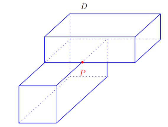
Figure 1: An example of a polyhedron satisfying (2.6) – (2.9) but not (2.10) at $P$. We refer the reader to [23, Example 3.7] for a detailed explanation, by using the uniform cone property, of the fact that $D$ is not a Lipschitz domain.

Let

$$\gamma_{D}:=1+(k-1)\chi_{D},$$ (2.11)

where $\chi_{D}$ is the characteristic function of $D\in\mathfrak{D}$, and $k$ is a positive constant such that

$$\min(k,|k-1|)\geq\kappa_{0}.$$ (2.12)

Finally let us state the assumptions on the part of the boundary on which we measure our data. Let $\Sigma$ be an open portion of $\partial\Omega$ with size at least $r_{0}$, i.e. we assume there exists at least one point $P_{\Sigma}\in\Sigma$ such that

$$dist(P_{\Sigma},\partial\Omega\setminus\Sigma)\geq r_{0}.$$ (2.13)

In the sequel, we will refer to the set of parameters

$$r_{0},\quad R_{0},\quad\theta_{0},\quad M_{0},\quad\kappa_{0}$$

as the a priori data.

2.2 The local Dirichlet to Neumann map

We define

$$H^{\frac{1}{2}}_{co}(\Sigma):=\Bigg{\{}\varphi\in H^{\frac{1}{2}}(\partial\Omega)\,:\,\textrm{supp}\ \varphi\subset\Sigma\Bigg{\}},$$

and with $H^{-\frac{1}{2}}_{co}(\Sigma)$ its topological dual.
Given $f\in H^{\frac{1}{2}}_{co}(\Sigma)$, we consider the boundary value problem

$$\begin{cases}\text{div}(\gamma_{D}\nabla u)=0&\textrm{in}\ \Omega\\ u=f&\textrm{on}\ \partial\Omega.\end{cases}$$ (2.14)

Let us denote by $\Lambda_{\gamma_{D}}^{\Sigma}$ the local DtN map, that is the map

$$\Lambda_{\gamma_{D}}^{\Sigma}:H^{\frac{1}{2}}_{co}(\Sigma) \to H^{-\frac{1}{2}}_{co}(\Sigma)$$ (2.15)

$$f \to\frac{\partial u}{\partial\nu}\bigg{\lfloor}_{\Sigma}$$

where $u\in H^{1}(\Omega)$ is the solution to (2.14), and $\nu$ is the outer unit normal vector to $\partial\Omega$. The norm of the local DtN map in the space of linear operators $\mathcal{L}\left(H^{\frac{1}{2}}_{co}(\Sigma),H^{-\frac{1}{2}}_{co}(\Sigma)\right)$ is defined by

$$\|\Lambda_{\gamma_{D}}^{\Sigma}\|_{\star}:=\textrm{sup}\bigg{\{}\|\Lambda_{\gamma_{D}}^{\Sigma}\varphi\|_{H^{-\frac{1}{2}}_{co}(\Sigma)}/\|\varphi\|_{H^{\frac{1}{2}}_{co}(\Sigma)}\,:\,\varphi\neq 0\bigg{\}}.$$

As in [10] the DtN map can be defined as the operator characterized by

$$\big{\langle}\Lambda_{\gamma_{D}}^{\Sigma}f,\phi\big{\rangle}=\int_{\Omega}\gamma_{D}\nabla u\cdot\nabla v\,dx,$$

for all $\phi,f\in H^{\frac{1}{2}}_{co}(\Sigma)$, where $u\in H^{1}(\Omega)$ is the solution to (2.14), and $v$ is any $H^{1}(\Omega)$-function such that $v\lfloor_{\Sigma}=\phi$.

2.3 The main result

Recalling the definition of the Hausdorff distance, see (1.4), we state here our main Lipschitz stability result:

Theorem 2.5.

Let $\Omega$ be a bounded domain with Lipschitz boundary satisfying (2.4), let $D_{0}$ and $D_{1}\in\mathfrak{D}$ (that is they satisfy assumptions (2.5)-(2.10)), let $k$ satisfy (2.12) and let $\Sigma$ be an open portion of $\partial\Omega$ satisfying (2.13). Then, there exists $C$ depending only on the a priori data such that

$$d_{H}\left(\partial D_{0},\partial D_{1}\right)\leq C\left\|\Lambda_{\gamma_{D_{0}}}^{\Sigma}-\Lambda_{\gamma_{D_{1}}}^{\Sigma}\right\|_{*},$$ (2.16)

where

$$\gamma_{D_{i}}=1+(k-1)\chi_{{D_{i}}}\quad\textrm{for}\quad i=0,1.$$

The proof of Theorem 2.5 is postponed at Section 6, after proving some intermediate results based essentially on the following steps and strategy:

1. Prove that it always exists a suitable tubular neighborhood connecting any point on $\partial\Omega$ to a special interior point of the face of one of the two polyhedra $D_{0}$ or $D_{1}$, without crossing $D_{0}\cup D_{1}$. To this aim, we introduce a specific distance (called “modified distance”) (see Definition 3.3) and exploit the connection between the modified and the Hausdorff distances (see Proposition 3.4).

2. The results of the previous point allow us to establish a rough (logarithmic) stability estimate of the Hausdorff distance between $D_{0}$ and $D_{1}$ in terms of the difference between the corresponding DtN map, see Theorem 4.5. This is obtained by propagating the smallness of data from $\Sigma$ along the tubular neighborhood.

3. The logarithmic stability estimate implies that if two DtN maps are close enough, the two polyhedra have the same number of vertices, faces and edges, see Proposition 3.9. When this happens, it is possible to define a regular vector field that transforms $D_{0}$ into $D_{1}$. We also prove smoothness of the local DtN map and establish a lower bound of its derivative with respect to the movement of the polyhedron

4. The regularity of the DtN map and the lower bound allow us to improve the stability estimates and to get Theorem 2.5.

3 Some useful geometric results on polyhedra

In this section we collect some geometric results on polyhedra in the class $\mathfrak{D}$. We first establish the relation between the Hausdorff distance of two polyhedra in $\mathfrak{D}$ and the Hausdorff distance of their boundaries, see Proposition 3.2. Afterwards, we consider a modified distance between two polyhedra (see Definition 3.3) that was introduced in [2, 9] and establish an upper bound of the Hausdorff distance of the boundaries of two polyhedra in terms of their modified distance, see Proposition 3.4. This last property together with the main result of this section, that is Proposition 3.8, will be crucial in Section 4 to establish our first logarithmic stability estimate.

Proposition 3.8 here corresponds to Lemma 4.2 in [9] where it is stated under the assumption of inclusions with $C^{1,\alpha}$ boundaries; this regularity assumption allows to show that the union of two such inclusions has Lipschitz boundary. Unfortunately, this is not the case for polyhedra in $\mathfrak{D}$. For this reason, in order to prove Proposition 3.8, we have to rely on a fine result from [39] stating that if two polyhedra in $\mathfrak{D}$ are close enough, in some neighborhood of some special point in the interior of one of the faces, the boundaries of the two polyhedra are relative graphs of affine functions (see Proposition 3.6).

The last key geometric result, contained in Proposition 3.9, states that if two polyhedra in $\mathfrak{D}$ are close enough, then they have the same number of vertices, edges and faces.

3.1 Metric results

In this subsection we use some results from [39]. For this, we observe that our class of polyhedra $\mathfrak{D}$ is a subset of the class of polyhedra $\mathcal{A}_{p,0}(h)$ (defined in [39]) for some $h>0$ depending only on the a priori data.

Let us set some useful notation. Given $P\in{\mathbb{R}}^{3}$, a direction $\nu\in{\mathbb{R}}^{3}$, $l>0$ and $\vartheta\in(0,\pi/2)$, we denote by

$$\mathcal{C}(P,\nu,l,\vartheta)=\left\{x\in{\mathbb{R}}^{3}\,:\,(x-P)\cdot\nu\geq|x-\overline{x}|\cos\vartheta,\,|x-P|\leq l\right\}$$ (3.1)

the closed cone with vertex $P$, axis $\nu$, width $\vartheta$, and apothem $l$.

Remark 3.1.

By assumption (2.10), for each $P\in\partial\left(\Omega\setminus D\right)$ there exist a direction $\nu$, a positive $l$ and $\vartheta\in(0,\pi/2)$ depending only on the a priori data, such that

$$\mathcal{C}(P,\nu,l,\vartheta)\subset\overline{(\Omega\setminus D)}$$

and, if $P\in\partial D$

$$\mathcal{C}(P,-\nu,l,\vartheta)\subset D.$$

The proposition below (that corresponds to Proposition 2.4 in [39] to which we refer for the proof) establishes the equivalence in $\mathfrak{D}$ between $d_{H}(D_{0},D_{1})$ and $d_{H}(\partial D_{0},\partial D_{1})$.

Proposition 3.2.

Let $D_{0}$ and $D_{1}\in\mathfrak{D}$, then there is a positive constant $C_{1}>1$ depending on the a priori data only such that

$$C_{1}^{-1}d_{H}(\partial D_{0},\partial D_{1})\leq d_{H}(D_{0},D_{1})\leq C_{1}d_{H}(\partial D_{0},\partial D_{1}).$$ (3.2)

For $D_{0}$ and $D_{1}\in\mathfrak{D}$, let $\mathcal{G}$ be the connected component of $\Omega\setminus\left(D_{0}\cup D_{1}\right)$ which contains $\partial\Omega$, and let

$$\Omega_{\mathcal{G}}=\Omega\setminus\mathcal{G}.$$ (3.3)

Since the value of $d_{H}(\partial D_{0},\partial D_{1})$ can be attained at some point of $\partial D_{0}\cup\partial D_{1}$ that is not necessarily on $\partial\Omega_{\mathcal{G}}$ (see, for example, the configuration in Figure 2) and, hence, cannot be reached from $\partial\Omega$ without crossing $\partial D_{0}\cup\partial D_{1}$, we introduce a modified distance as was defined in [9].

Definition 3.3.

$$d_{\mu}(D_{0},D_{1})=\max\left\{\max_{x\in\partial D_{0}\cap\partial\Omega_{\mathcal{G}}}dist(x,D_{1}),\max_{x\in\partial D_{1}\cap\partial\Omega_{\mathcal{G}}}dist(x,D_{0})\right\}.$$ (3.4)

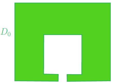
(a) Polyhedron $D_{0}$ in green.

(b) Polyhedron $D_{1}$ in pale blue.

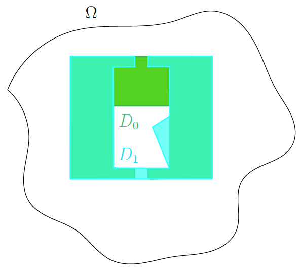
(c) A possible configuration. The two polyhedra are overlapping.

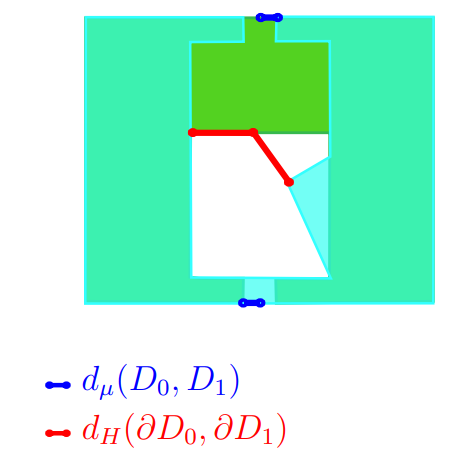
(d) The two distances. For $d_{H}$ we provide all the points where the longest distance between the two sets occurs.

Figure 2: A 2D-section of a possible geometrical setting. Note that Figure 2(d) represents the case when the value of $d_{H}(\partial D_{0},\partial D_{1})$ is attained at some point that is not on $\partial\Omega_{\mathcal{G}}$.

We point out that this is not a metric because, in general, the triangle inequality doesn’t hold. It is straightforward to show, see [9], that

$$d_{\mu}(D_{0},D_{1})\leq d_{H}(\partial D_{0},\partial D_{1}).$$ (3.5)

In general, $d_{\mu}$ does not bound from above the Hausdorff measure, but, in the class $\mathfrak{D}$ the following result that will be crucial for deriving the stability estimates in Section 4, holds:

Proposition 3.4.

There is a constant $C_{2}>1$ depending only on the a priori data, such that, for $D_{0}$, $D_{1}\in\mathfrak{D}$

$$d_{H}(\partial D_{0},\partial D_{1})\leq C_{2}d_{\mu}(D_{0},D_{1}).$$

In order to prove Proposition 3.4 we need the following preliminary result:

Lemma 3.5.

Let $D\in\mathfrak{D}$. Then, for every $P\in\partial D$ there exists a curve $\mathfrak{c}$ in $\Omega\setminus D$ connecting $P$ to $\partial\Omega$ such that

$$|z-P|\leq C_{2}\,dist(z,D),\quad{\forall z\in\mathfrak{c}},$$

where $C_{2}>1$ depends only on the a priori data.

This lemma corresponds to Proposition 3.3 in [8] and to Lemma 4.1 in [9] for $C^{1,\alpha}$ inclusions. Here, we prove it for $D\in\mathfrak{D}$.

Proof of Lemma 3.5.

By Assumption (2.10) we can apply Lemma 5.5 in [11], hence, there exists a positive number $a$ depending only on the Lipschitz constant $M_{0}$ such that the set

$$E^{D}_{t}=\left\{x\in\overline{\Omega}\setminus D\,:\,dist(x,\partial D)>t\right\}$$ (3.6)

is connected for $t\leq ar_{0}$.

Let $P\in\partial D$; by Remark 3.1, there exists a cone $\mathcal{C}(P,\nu,l,\vartheta)\subset\overline{(\Omega\setminus D)}$. By easy calculations we can see that, by choosing

$$\tau_{0}=\frac{l}{1+\sin\vartheta},$$

the point $y_{\tau_{0}}=P+\tau_{0}\nu$ satisfies $dist\left(y_{\tau_{0}},\partial C(P,\nu,l,\vartheta\right))=\tau_{0}\sin\vartheta$. Let us now take $t_{0}=\min\left\{ar_{0},\tau_{0}\right\}$. Since $t_{0}\leq\tau_{0}$, we have

$$dist\left(y_{t_{0}},\Omega\setminus D\right)\geq dist\left(y_{t_{0}},\partial\mathcal{C}(P,\nu,l,\vartheta)\right)\geq t_{0}\sin\vartheta,$$

hence $y_{t_{0}}\in E^{D}_{t_{0}\sin\vartheta}$. Since $t_{0}\sin\vartheta<ar_{0}$, then $E^{D}_{t_{0}\sin\vartheta}$ is connected.

Let $\mathfrak{c}^{\prime}$ be a curve in $E^{D}_{t_{0}\sin\vartheta}$ that connects $y_{t_{0}}$ to $\partial\Omega$ and let $\mathfrak{c}=\mathfrak{c}^{\prime}\cup[y_{t_{0}},P]$, where $[y_{t_{0}},P]$ is the line segment from $P$ to $y_{t_{0}}$.

If $z\in\mathfrak{c}^{\prime}$, then $dist(z,\partial D)\geq t_{0}\sin\vartheta$, hence

$$|z-P|\leq diam(\Omega)\leq R_{0}\leq\frac{R_{0}}{t_{0}\sin\vartheta}dist(z,\partial D).$$

If $z\in[y_{t_{0}},P]$, then $dist(z,\partial D)\geq|z-P|\sin\vartheta$. In both cases

$$|z-P|\leq\max\left\{\frac{R_{0}}{t_{0}\sin\vartheta},\frac{1}{\sin\vartheta}\right\},\quad\forall z\in\mathfrak{c}.$$

∎

We are now ready to prove Proposition 3.4.

Proof of Proposition 3.4.

Let $P\in\partial D_{0}$, we have two different cases

1. $P\in\partial D_{0}\cap\partial\Omega_{\mathcal{G}}$;

2. $P\in\partial D_{0}\setminus\partial\Omega_{\mathcal{G}}$.

In case (i) we have that $P\notin Int(D_{1})$, hence

$$dist(P,\partial D_{1})=dist(P,D_{1})\leq d_{\mu}(D_{0},D_{1}).$$

In case (ii) we have $P\in Int(\Omega_{\mathcal{G}})$. By Lemma 3.5, let $\mathfrak{c}$ be a curve such that

$$\mathfrak{c}\subset\Omega\setminus D_{0}$$

connects $P$ to $\partial\Omega$ and

$$|z-P|\leq C_{2}dist(z,D_{0}),\quad\forall z\in\mathfrak{c}.$$ (3.7)

Since $P\in Int(\Omega_{\mathcal{G}})$, $\mathfrak{c}$ intersects $\partial\Omega_{\mathcal{G}}$ and, since

$$\left(\mathfrak{c}\cap\partial D_{0}\right)\setminus\{P\}=\emptyset,$$

then

$$\left(\mathfrak{c}\cap\Omega_{\mathcal{G}}\right)\cap\partial D_{1}\neq\emptyset.$$

Let $\overline{z}\in\mathfrak{c}\cap\partial\Omega_{\mathcal{G}}\cap\partial D_{1}$. We have

$$dist(\overline{z},D_{0})\leq\sup_{x\in\partial D_{1}\cap\partial\Omega_{\mathcal{G}}}dist(x,D_{0})\leq d_{\mu}(D_{0},D_{1})$$

and, by (3.7), we have

$$\frac{1}{C_{2}}|\overline{z}-P|\leq dist(\overline{z},D_{0})\leq d_{\mu}(D_{0},D_{1}).$$ (3.8)

Since $\overline{z}\in\partial D_{1}$ and by (3.7)

$$dist(P,\partial D_{1})\leq|\overline{z}-P|,$$ (3.9)

hence, from (3.8) and (3.9) we have

$$dist(P,\partial D_{1})\leq C_{2}d_{\mu}(D_{0},D_{1}),\quad\forall P\in\partial D_{0},$$ (3.10)

and, by symmetry,

$$dist(Q,\partial D_{0})\leq C_{2}d_{\mu}(D_{0},D_{1}),\quad\forall Q\in\partial D_{1}.$$ (3.11)

Inequalities (3.10) and (3.11) imply that

$$d_{H}(\partial D_{0},\partial D_{1})\leq C_{2}d_{\mu}(D_{0},D_{1}).$$

∎

3.2 A useful geometric construction

The aim of this subsection (see Proposition 3.8) is the construction of a special tubular set contained in $\mathcal{G}$ that connects a special point on $\partial\Omega_{\mathcal{G}}$ to any point on $\partial\Omega$ (and particularly any point on $\Sigma$) and has a fixed positive distance from the rest of the boundaries of the two polyhedra. In this set we will be able to propagate the information on the DtN map up the the boundary of $\partial\Omega_{\mathcal{G}}$.

In order to construct this tubular set, we need some information on the position of the boundaries of the two polyhedra when they are sufficiently close. Proposition 3.6 below, that is the adaptation to our setting of Proposition 6.2 in [39], states that, in a neighborhood of some point, the boundaries of the two polyhedra are relative graphs of affine functions that are not too close (see (3.12)) .

Proposition 3.6.

There exist positive constants $k_{1}\leq\overline{k}_{0}\leq k_{0}$, $K$, $K_{1}$ and $L_{1}$ depending only on the a priori data, such that, if $D_{0}$, $D_{1}\in\mathfrak{D}$ and

$$d_{H}(D_{0},D_{1})\leq k_{0}r_{0},$$

then there exist $P_{0}\in\partial D_{0}$ and $P_{1}\in\partial D_{1}$ such that the following conditions are satisfied. Up to a rigid transformation $P_{0}=(0,0,0)$, $P_{1}=(0,0,a_{1})$ and

$$\partial D_{0}\cap B_{\overline{k}_{0}r_{0}}=\left\{(x_{1},x_{2},x_{3})\in B_{\overline{k}_{0}r_{0}}\,:\,x_{3}=\Phi_{0}(x_{1},x_{2})\right\},$$

$$\partial D_{1}\cap B_{\overline{k}_{0}r_{0}}=\left\{(x_{1},x_{2},x_{3})\in B_{\overline{k}_{0}r_{0}}\,:\,x_{3}=\Phi_{1}(x_{1},x_{2})\right\},$$

where $\Phi_{0}$ and $\Phi_{1}$ are Lipschitz functions with Lipschitz constant bounded by $L_{1}$ and such that $\Phi_{0}(0,0)=0$ and $\Phi_{1}(0,0)=a_{1}$.

Furthermore, on $B_{k_{1}r_{0}}^{\prime}=\left\{(x_{1},x_{2})\in{\mathbb{R}}^{2}\,:\,x_{1}^{2}+x_{2}^{2}\leq k_{1}^{2}r_{0}^{2}\right\}$ we have

$$\Phi_{0}(x_{1},x_{2})=l^{0}_{1}x_{1}+l^{0}_{2}x_{2},\quad\Phi_{1}(x_{1},x_{2})=l^{1}_{1}x_{1}+l^{1}_{2}x_{2}\quad\forall(x_{1},x_{2})\in B_{k_{1}r_{0}}^{\prime}$$

$$S_{0}=\left\{(x_{1},x_{2},\Phi_{0}(x_{1},x_{2})\,:\,(x_{1},x_{2})\in B_{k_{1}r_{0}}^{\prime}\right\}\subset\partial D_{0},$$

$$S_{1}=\left\{(x_{1},x_{2},\Phi_{1}(x_{1},x_{2})\,:\,(x_{1},x_{2})\in B_{k_{1}r_{0}}^{\prime}\right\}\subset\partial D_{1},$$

$$(l^{0}_{1}-l^{1}_{1})^{2}+(l^{0}_{2}-l^{1}_{2})^{2}\leq\left(\frac{Kd_{H}(D_{0},D_{1})}{r_{0}}\right)^{2},$$

$$|a_{1}|\leq Kd_{H}(D_{0},D_{1}),$$

and

$$\left|\Phi_{0}(x_{1},x_{2})-\Phi_{1}(x_{1},x_{2})\right|\geq K_{1}(d_{H}(D_{0},D_{1}))^{3},\quad\forall(x_{1},x_{2})\in B_{k_{1}r_{0}}^{\prime}.$$ (3.12)

Remark 3.7.

Notice that $k_{0}$ can be chosen such that $D_{0}$ and $D_{1}$ are on the same side with respect to $S_{0}$ and $S_{1}$.

We call $D_{0}$ the polyhedron for which the point $P_{0}\in\partial\Omega_{\mathcal{G}}$.

Let us now introduce the description of a tubular neighborhood of a curve as was introduced in [12, 9]. Let $P\in\partial\Omega_{\mathcal{G}}$ and let $\nu$ be a unit direction such that the line segment $[P,P+d\nu]$ is contained in $\mathcal{G}$ for some $d>0$. Let $\overline{P}$ be a point on $\partial\Omega$, consider a curve $\mathfrak{c}$ joining $\overline{P}$ to $P+d\nu$ and define, for some $R\in(0,d)$

$$V_{R}(\mathfrak{c})=\bigcup_{Q\in\mathfrak{c}}B_{R}(Q)\bigcup\mathcal{C}\left(P,\nu,\frac{d^{2}-R^{2}}{d},\arcsin\frac{R}{d}\right)$$

where $\mathcal{C}$ is the cone defined in (3.1).

In the next proposition, we show that such a set $V_{R}(\mathfrak{c})$ can be constructed in $\mathcal{G}$, see, for example, Figure 3.

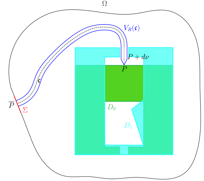
Figure 3: A 2D-section of a possible configuration with the representation of $V_{R}(\mathfrak{c})$ and $\mathfrak{c}$ connecting $\overline{P}$ to $P+d\nu$.

Proposition 3.8.

If $D_{0}$, $D_{1}\in\mathfrak{D}$, there exist constants $C_{3}$, $d$, $R$ (with $R<d$) and $R_{1}$ depending only on the a priori data and there is a point $P\in\partial D_{0}\cap\partial\Omega_{\mathcal{G}}$ such that

$$C_{3}d_{\mu}^{3}(D_{0},D_{1})\leq dist(P,D_{1}),$$ (3.13)

$$dist(P,\{\sigma^{D_{0}}_{ij}\}_{i\neq j})\geq R_{1},$$ (3.14)

and such that, given any point $\overline{P}\in\partial\Omega$ there is a curve $\mathfrak{c}$ joining $\overline{P}$ to $P+d\nu$, where $\nu$ is the unit outer normal to $\partial D_{0}$, such that

$$V_{R}(\mathfrak{c})\subset\overline{\mathcal{G}}.$$ (3.15)

Proof.

Let us denote by $d_{\mu}=d_{\mu}(D_{0},D_{1})$ and let

$$d_{1}=\frac{r_{0}}{2C_{1}C_{2}}\min\left\{k_{1},a\right\}.$$

We distinguish two cases.

Case 1: $d_{\mu}\geq d_{1}$.
Note that, by Lemma 5.5 in [11], the sets $E_{t}^{D_{0}}$ and $E_{t}^{D_{1}}$ (defined as in (3.6)) are connected for $t\leq d_{1}\leq ar_{0}$.

Let $\widetilde{P}$ be a point on $\partial D_{0}\cap\partial\Omega_{\mathcal{G}}$ be the point that satisfies

$$d_{\mu}(D_{0},D_{1})=dist(\widetilde{P},D_{1}).$$

Let $P$ be a point in the face containing $\widetilde{P}$ (or in one of the faces containing $\widetilde{P}$) such that

$$dist(P,\{\sigma_{ij}^{D_{0}}\}_{i\neq j})\geq\frac{d_{1}}{4}\sin\left(\frac{\theta_{0}}{2}\right)$$

and

$$dist(P,D_{1})\geq\frac{d_{1}}{2}.$$ (3.16)

Consider the outer cone to $D_{0}$ at $P$ (see Remark 3.1). Since $P$ is internal to a face, the direction $\nu$ can be chosen orthogonal to $\partial D_{0}$.

The point $P+\frac{d_{1}}{4}\nu$ belongs to $E_{D_{1}}^{\frac{d_{1}}{2}}$ and also to $E_{D_{0}}^{\frac{d_{1}}{4}\sin\vartheta}$ (with $\vartheta$ from Remark 3.1).

Then, given any point $\overline{P}\in\partial\Omega$ there is a curve $\mathfrak{c}$ joining $P+\frac{d_{1}}{4}\nu$ to $\overline{P}$ with distance bigger than $\frac{d_{1}}{4}\sin\vartheta$ from $\Omega_{\mathcal{G}}$.

Moreover we trivially have

$$d_{\mu}^{3}(D_{0},D_{1})\leq(diam(\Omega))^{3}\leq R_{0}^{3},$$

hence, by (3.16)

$$d_{\mu}^{3}(D_{0},D_{1})\leq R_{0}^{3}\frac{2dist(P,D_{1})}{d_{1}}$$

that gives (3.13).

Case 2: $d_{\mu}<d_{1}$
Since by Proposition 3.2 and Proposition 3.4

$$d_{H}(D_{0},D_{1})\leq C_{1}C_{2}d_{\mu}(D_{0},D_{1})$$

we have

$$d_{H}(D_{0},D_{1})\leq C_{1}C_{2}d_{1}\leq k_{0}r_{0}$$

so that the assumptions of Proposition 3.6 hold true.

Let now $P_{0}$ be the point in Proposition 3.6 and let $\nu_{0}$ be the normal direction to $S_{0}$ (defined in Proposition 3.6). Notice that, due to (3.12) the cone of $\mathcal{C}(P_{0},\nu_{0},k_{1}r_{0},\pi/2)$ is contained in $\mathcal{G}$.
Let us take the point $P_{0}+\frac{k_{1}r_{0}}{2}\nu_{0}$ and notice that

$$dist\left(P_{0}+\frac{k_{1}r_{0}}{2}\nu_{0},D_{0}\right)=\frac{k_{1}r_{0}}{2}.$$

Let $t_{0}=\min\{\frac{k_{1}r_{0}}{2},ar_{0}\}$ so that $E_{t_{0}}^{D_{0}}$ is connected.

Let $\mathfrak{c}$ be a curve joining $P_{0}+\frac{k_{1}r_{0}}{2}\nu_{0}$ to a point $\overline{P}\in\partial\Omega$ and such that $\mathfrak{c}\subset E_{t_{0}}^{D_{0}}$. By choosing $d=\frac{k_{1}r_{0}}{2}$ and $R=t_{0}/4$ the tubular set $V_{R}(\mathfrak{c})$ (starting from $P=P_{0}$) is contained in $\overline{\Omega\setminus D_{0}}$.

Now, since

$$d_{H}(D_{0},D_{1})\leq C_{1}C_{2}d_{1}\leq\frac{t_{0}}{2}$$

the set $V_{R}(\mathfrak{c})$ is contained also in $\overline{\Omega\setminus D_{1}}$, and (3.15) follows.

Inequalities (3.13) and (3.14) (for $P=P_{0}$ and $R_{1}=k_{0}r_{0}$) are a straightforward consequence of (3.12), (3.5) and (3.2). ∎

3.3 Estimating the distance between vertices of close polyhedra

We now state and prove the main result of the section: if two polyhedra in $\mathfrak{D}$ are close enough, then they have the same number of vertices (and faces and edges).

Proposition 3.9.

There exist two positive constants $\delta_{0}$ and $C$ depending only on the a priori data, such that, if for some $D_{0}$ and $D_{1}$ in $\mathfrak{D}$,

$$d_{H}\left(\partial D_{0},\partial D_{1}\right)\leq\delta_{0},$$

then $D_{0}$ and $D_{1}$ have the same number $N$ of vertices $\left\{V^{D_{0}}_{i}\right\}_{i=1}^{N}$ and $\left\{V^{D_{1}}_{i}\right\}_{i=1}^{N}$, respectively, which can be ordered in such a way that

$$dist\left(V^{D_{0}}_{i},V^{D_{1}}_{i}\right)\leq Cd_{H}\left(\partial D_{0},\partial D_{1}\right).$$ (3.17)

Moreover, for each edge or face in $D_{0}$ there is an edge or a face in $D_{1}$ with corresponding vertices.

Proof.

The proof of Proposition 3.9 follows the same idea of the proof of Proposition 3.3 in [20] in the two dimensional setting. In that case we show that, if the Hausdorff distance between the boundaries is small enough, a vertex of one of the two polygons cannot be too far from vertices of the other polygon without violating the a priori assumptions.

For polyhedra the proof is more involved and it is divided in two steps: in the first step we show that the distance between an arbitrary vertex in $D_{0}$ from the edges of $D_{1}$ can be bounded by $Cd_{H}\left(\partial D_{0},\partial D_{1}\right)$ where $C$ depends only on the a priori data. The main idea to prove this consists in showing that a small neighborhood of a face of one polyhedron cannot contain a vertex of the second polyhedron since the length of edges and width of angles are bounded from below by the a priori data.

In the second step, we show that an arbitrary vertex of $D_{0}$ has distance smaller than $Cd_{H}\left(\partial D_{0},\partial D_{1}\right)$ from a vertex in $D_{1}$. This time the idea is that a small neighborhood of a pair of intersecting faces cannot contain a vertex that does not violate assumption (2.9). Since assumption (2.8) holds, if $d_{H}\left(\partial D_{0},\partial D_{1}\right)$ is small enough there is a one to one correspondence between vertices of the two polyhedra.

For sake of brevity let us denote by

$$d_{H}=d_{H}\left(\partial D_{0},\partial D_{1}\right),$$ (3.18)

and let

$$\left(\partial D_{1}\right)^{(d_{H})}=\left\{x\in{\mathbb{R}}^{3}\,:\,dist(x,\partial D_{1})\leq d_{H}\right\}.$$

By definition of Hausdorff distance it follows that $\partial D_{0}\subset\left(\partial D_{1}\right)^{(d_{H})}$.

We can also assume that $\left(\Omega\right)_{d_{H}}\setminus\left(\partial D_{1}\right)^{(d_{H})}$ is connected by [9, Lemma 5.5], where

$$\left(\Omega\right)_{d_{H}}=\left\{x\in\Omega\,:\,dist(x,\partial\Omega)>d_{H}\right\}.$$

Let us choose an arbitrary vertex in $D_{0}$ and let us denote it by $V_{1}^{D_{0}}$. Let $F_{i}^{D_{1}}$ be a face of $D_{1}$ such that

$$dist(V_{1}^{D_{0}},F_{i}^{D_{1}})\leq d_{H}$$

(notice that such a face exists because $V_{1}^{D_{0}}\in\left(\partial D_{1}\right)^{(d_{H})}$).

Let us choose our coordinate system such that $V_{1}^{D_{0}}=(0,0,0)$, and $F_{i}^{D_{1}}$ lies on the plane $\{x_{3}=-c\}$ for $0\leq c\leq d_{H}$.

We now want to show that there exists a vertex (say $V_{1}^{D_{1}}$) of the polygon $F_{i}^{D_{1}}$ such that

$$dist(V_{1}^{D_{0}},V_{1}^{D_{1}})\leq Cd_{H}$$

where $C$ depends only on the a priori assumptions.

First step. Let us show that there exists $C_{0}$, depending only on the a priori data, such that, if $d_{H}$ is small enough, then

$$dist((0,0,-c),\partial F_{i}^{D_{1}})\leq C_{0}d_{H}$$ (3.19)

and, hence, since $0\leq c\leq d_{H}$

$$dist(V_{1}^{D_{0}},\partial F_{i}^{D_{1}})\leq(C_{0}+1)d_{H}.$$ (3.20)

In order to prove (3.19), let us assume that

$$dist((0,0,-c),\partial F_{i}^{D_{1}})>C_{0}d_{H}$$ (3.21)

and show that there is a constant $C_{0}$ such that (3.21) leads to a contradiction for sufficiently small $d_{H}$.

By assumption (2.9), the cones with basis $B^{\prime}_{C_{0}d_{H}}\left((0,0,-c)\right)$ and height $C_{0}d_{H}\tan\theta_{0}$ do not intersect other faces of $D_{1}$ except $F_{i}^{D_{1}}$.

Let us take $C_{0}>\frac{1+\cos\theta_{0}}{\sin\theta_{0}}$. It is easy to show that the ball centered at $V_{1}^{D_{0}}$ with radius $C_{1}d_{H}$, where $C_{1}=\frac{1}{2}\left(C_{0}\sin\theta_{0}-\cos\theta_{0}-1\right)$ does not intersect the set

$$\left\{x\in{\mathbb{R}}^{3}\,:\,dist\left(x,\partial D_{1}\setminus F_{i}^{D_{1}}\right)\leq d_{H}\right\}.$$

Let us now take $d_{H}$ such that $C_{1}d_{H}<r_{0}$. This implies that the edges of $D_{0}$ that contain $V_{1}^{D_{0}}$, that are contained in $\left(\partial D_{1}\right)^{(d_{H})}$, by definition of the Hausdorff measure, intersect $\partial B_{C_{1}d_{H}}\left(V_{1}^{D_{0}}\right)$ at points that lie between the planes $\pi^{+}=\left\{x_{3}=2d_{H}\right\}$ and $\pi^{-}=\left\{x_{3}=-2d_{H}\right\}$ (as a matter of fact the region on the ball that can contain these intersections is smaller, but we choose this one to have a symmetric one).

Figure 4: First step of the proof. Note that if the strip is too small then the vectors are not all contained in it.

Let $\sigma_{ij}^{D_{0}}$ be one of the edges of $D_{0}$ that contains $V_{1}^{D_{0}}$ and let us denote by $v$ the position vector that represents the intersection of this edge with the sphere $B_{C_{1}d_{H}}\left(V_{1}^{D_{0}}\right)$.

Let $u$ and $w$ the position vectors with tips at the intersection of the edges of the faces of $D_{0}$ adjacent to $\sigma_{ij}^{D_{0}}$ with $\partial B_{C_{1}d_{H}}\left(V_{1}^{D_{0}}\right)$

We have that

$$\begin{split}|u|=|v|=|w|=C_{1}d_{H},\\ |u_{3}|,\,|v_{3}|,\,|w_{3}|\leq 2d_{H}.\end{split}$$ (3.22)

Let $\theta_{ij}$ denote the internal angle at the edge $\sigma_{ij}^{D_{0}}$. We now show that, if $C_{1}$ (and, hence, if $C_{0}$) is big enough and $C_{1}d_{H}<r_{0}$, then

$$|\cos\theta_{ij}|>\cos\theta_{0}$$

in contradiction with assumption (2.9).

Let us consider the unit normal direction to the faces intersecting at $\sigma_{ij}^{D_{0}}$:

$$t=\frac{u\times v}{|u\times v|}\mbox{ and }\tau=\frac{v\times w}{|v\times w|}.$$ (3.23)

Notice that, by (3.22),

$$|u\times v|^{2} \leq (u_{1}^{2}+u_{2}^{2}+v_{1}^{2}+v_{2}^{2})(u_{3}^{2}+v_{3}^{2})+(u_{1}v_{2}-u_{2}v_{1})^{2}$$

$$\leq 16C_{1}^{2}d_{H}^{4}+t_{3}^{2}|u\times v|^{2},$$

so that

$$(1-t_{3}^{2})|u\times v|^{2}\leq 16C_{1}^{2}d_{H}^{4}.$$ (3.24)

From assumption (2.6) and (3.22) we have

$$|u\times v|^{2}=|u|^{2}|v|^{2}|\sin\hat{uv}|^{2}\geq(C_{1}d_{H})^{4}\sin^{2}\theta_{0}.$$ (3.25)

From (3.24) and (3.25),

$$1-t_{3}^{2}\leq\frac{16}{C_{1}^{2}\sin^{2}\theta_{0}},$$

hence

$$1-|t_{3}|\leq\frac{16}{C_{1}^{2}\sin^{2}\theta_{0}}$$ (3.26)

and, in the same way,

$$1-|\tau_{3}|\leq\frac{16}{C_{1}^{2}\sin^{2}\theta_{0}}.$$ (3.27)

Now, by (3.26) and (3.27),

$$|\cos\theta_{ij}| = |t\cdot\tau|\geq|t_{3}||\tau_{3}|-|t^{\prime}||\tau^{\prime}|$$ (3.28)

$$= |t_{3}||\tau_{3}|-\sqrt{(1-|t_{3}|^{2})(1-|\tau_{3}|^{2})}\geq 1-\frac{48}{C_{1}^{2}\sin^{2}\theta_{0}}.$$ (3.29)

For this reason, if

$$C_{1}^{2}>\frac{48}{(1-\cos\theta_{0})\sin^{2}\theta_{0}},$$ (3.30)

we have that

$$|\cos\theta_{ij}|>\cos\theta_{0}$$

that contradicts (2.9).

So, let us take, for example

$$C_{0}=2\left\{\frac{8\sqrt{3}}{\sqrt{1-\cos\theta_{0}}\sin^{2}\theta_{0}}+\frac{1+\cos\theta_{0}}{\sin\theta_{0}}\right\}.$$

With this choice, (3.30) holds, hence we have a contradiction for $d_{H}<\frac{r_{0}}{C_{1}}$. This implies that, for $d_{H}<\frac{r_{0}}{C_{1}}$, (3.19) and (3.20) hold.

Second step. Since (3.20) holds, there is an edge $\sigma_{ij}^{D_{1}}$ such that

$$dist\left(V_{1}^{D_{0}},\sigma_{ij}^{D_{1}}\right)\leq(C_{0}+1)d_{H}.$$

Let $V_{1}^{D_{1}}$ and $V_{2}^{D_{1}}$ be the endpoints of $\sigma_{ij}^{D_{1}}$.

We want to show that there is $C_{2}$ depending only on the a priori data, such that, for $d_{H}$ small enough, either

$$dist\left(V_{1}^{D_{0}},V_{1}^{D_{1}}\right)\leq C_{2}d_{H}\mbox{ or }dist\left(V_{1}^{D_{0}},V_{2}^{D_{1}}\right)\leq C_{2}d_{H}.$$

Again, we proceed by contradiction and assume that

$$dist\left(V_{1}^{D_{0}},V_{1}^{D_{1}}\right)>C_{2}d_{H}\mbox{ and }dist\left(V_{1}^{D_{0}},V_{2}^{D_{1}}\right)>C_{2}d_{H}.$$

and get a contradiction with the a priori assumptions on $\mathfrak{D}$, see Figure 5.

(a) Geometrical setting.

(b) A partial $d_{H}$-neighborhood of the two faces $F^{D_{1}}_{i}$ and $F^{D_{1}}_{j}$.

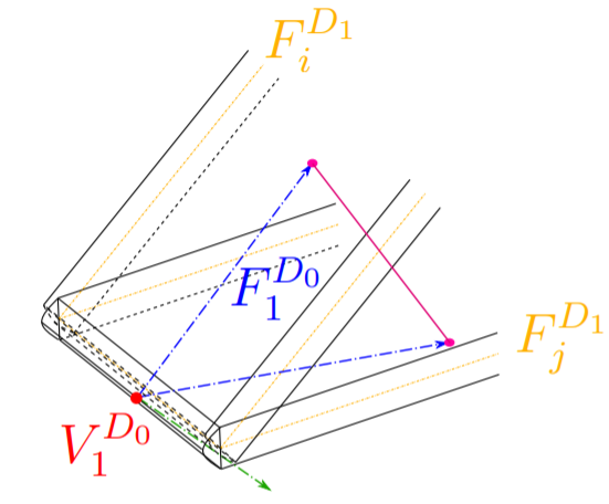
(c) The two edges in blue of the face $F^{D_{0}}_{1}$.

Figure 5: A sketch of the geometrical setting for the second step of the proof.

Let $F_{j}^{D_{1}}$ be such that $F_{i}^{D_{1}}\cap F_{j}^{D_{1}}=\sigma_{ij}^{D_{1}}$.

As in the first step, by elementary calculations, there is a ball centered at $V_{1}^{D_{0}}$ of radius $C_{3}d_{H}$, where $C_{3}$ depends on the a priori data and on $C_{2}$, such that

$$B_{C_{3}d_{H}}\left(V_{1}^{D_{0}}\right)\cap\left\{x\in{\mathbb{R}}^{3}\,:\,dist\left(x,\partial D_{1}\setminus\left(F_{i}^{D_{1}}\cup F_{j}^{D_{1}}\right)\right)\leq d_{H}\right\}=\emptyset.$$

This implies that the intersections of all the edges containing $V_{1}^{D_{0}}$ with such ball lie in a $d_{H}$-neighborhood of the two faces. From the first step, we know that, it is not possible to have all these intersections in the neighborhood of only one of the two faces. Hence, there is a face (say $F_{1}^{D_{0}}$) containing $V_{1}^{D_{0}}$ that has one edge in the neighborhood of $F_{i}^{D_{1}}$ and one in $F_{j}^{D_{1}}$. With calculations similar to the ones in the first step, that we omit for sake of shortness, it is possible to show that, for $C_{2}$ big enough, a part of the face $F_{1}^{D_{0}}$ does not belong to $\left(\partial D_{1}\right)^{(d_{H})}$ contradicting the definition of the Hausdorff distance. ∎

4 A first rough stability estimate

In this section we derive a rough stability estimate of polyhedral inclusions measured in the Hausdorff distance in terms of the operator norm of the partial DtN map. As shown in the previous section, this estimate is crucial to prove that the two polyhedra have the same vertices which can be ordered in such a way that they are close, see Proposition 3.9.

4.1 On some properties of the Green’s function

Let us first recall Alessandrini’s identity. Let $u_{0}$ and $u_{1}$, with $\textrm{supp}(u_{0}\lfloor_{\partial\Omega})$, $\textrm{supp}(u_{1}\lfloor_{\partial\Omega})\subset\Sigma$, be solutions of the equations

$$\text{div}(\gamma_{D_{i}}\nabla u_{i})=0,\qquad i=0,1,$$

and $\Lambda_{\gamma_{D_{i}}}^{\Sigma}$ the corresponding local DtN maps, for $i=0,1$. Then, it holds

$$\big{\langle}(\Lambda_{\gamma_{D_{0}}}^{\Sigma}-\Lambda_{\gamma_{D_{1}}}^{\Sigma})u_{0}\big{\lfloor}_{\Sigma},u_{1}\big{\lfloor}_{\Sigma}\big{\rangle}=\int_{\Omega}(k-1)(\chi_{D_{0}}-\chi_{D_{1}})\nabla u_{0}\cdot\nabla u_{1}\,dx,$$ (4.1)

where $\chi_{D_{i}}$, for $i=0,1$, is the characteristic function of $D_{i}$.

As in [10, 11], we introduce an augmented domain $\Omega^{\sharp}$, attaching to $\Omega$ an open set $\Omega_{0}$, in its exterior, whose boundary intersects $\partial\Omega$ on an open portion $\Sigma_{0}\Subset\Sigma$ such that $\Sigma_{0}$ has size which is a fraction of $r_{0}$. Let us choose $\Omega_{0}$ in such a way that $\Omega^{\sharp}:=\Omega\cup\Sigma_{0}\cup\Omega_{0}$ has the following properties: there exist $r_{1}$, $M_{1}$, depending only on $r_{0}$, and $M_{0}$ such that

1. $\Omega^{\sharp}$ is open, connected with Lipschitz boundary with constants $r_{1}$, $M_{1}$;

2. there exists $P_{0}\in\Omega_{0}$ such that

   $$B_{2r_{1}}(P_{0})\subset\Omega_{0}.$$ (4.2)

We extend the conductivity to be $1$ in $\Omega_{0}$ still denoting it with $\gamma_{D}$.
Let $\Gamma(x,y)$ be the fundamental solution of the Laplace operator, that is the function

$$\Gamma(x,y)=\frac{1}{4\pi}\frac{1}{|x-y|},$$

and with $G^{\sharp}$ the Green’s function, solution to

$$\begin{cases}\text{div}(\gamma_{D}\nabla G^{\sharp}(\cdot,y))=-\delta(\cdot-y)&\textrm{in}\ \Omega^{\sharp}\\ G^{\sharp}(\cdot,y)=0&\textrm{on}\ \partial\Omega^{\sharp},\end{cases}$$ (4.3)

where $\delta(\cdot-y)$ is the Dirac distribution centered in $y$. Let us recall some properties of the Green function. For all $x,y\in\Omega^{\sharp},\ x\neq y$, it holds

$$G^{\sharp}(x,y)= G^{\sharp}(y,x)$$

$$0<G^{\sharp}(x,y)\leq \frac{c}{|x-y|},$$

where $c$ depends only on $k$, see [13]. Fix a point $y\in\Omega^{\sharp}\setminus D$ and let $0<r_{2}=dist(y,\{\sigma_{ij}^{D}\}_{i\neq j}\cup\partial\Omega^{\sharp})$, for $i,j=1,\cdots,H$. Then, there exists a constant $C>1$ depending only on the a priori data such that $B_{r_{2}/C}(y)$ contains at most a portion of one face of the polyhedron $D$. Hence, in this case, the ball is divided into two zones with different conductivity coefficient (thanks to (2.11)), that is, for a suitable coordinate system, there exists $a\in[-\frac{r_{2}}{C},\frac{r_{2}}{C}]$ such that

$$\widehat{\gamma}_{D}(x)=1+(k-1)\chi_{\{x_{3}>a\}}(x),\qquad\forall x\in B_{r_{2}/C}(y).$$ (4.4)

We extend the coefficient $\widehat{\gamma}_{D}$ in $\mathbb{R}^{3}$, that is, we define

$$\widehat{\gamma}_{y}(x):=1+(k-1)\chi_{\{x_{3}>a\}}(x),\qquad\forall x\in\mathbb{R}^{3},$$

where the same coordinate frame of (4.4) has been used. Denote by $\widehat{\Gamma}$ the biphase fundamental solution of

$$\text{div}(\widehat{\gamma}_{y}(\cdot)\nabla\widehat{\Gamma}(\cdot,y))=-\delta(\cdot-y),\qquad\textrm{in}\ \mathbb{R}^{3}.$$

We refer the reader to [13] for more details on the biphase fundamental solution. In the following proposition, we recall other useful properties of the Green function that come from some of the results in [13, 17, 18].

Proposition 4.1.

For all $C_{1}>1$ there exists a constant $C>0$ depending on the a priori data and $C_{1}$ such that, for all $y\in\Omega^{\sharp}\setminus D$ satisfying

$$dist(y,\{\sigma_{ij}^{D}\}_{i\neq j}\cup\partial\Omega^{\sharp})\geq\frac{r_{0}}{C_{1}},\qquad i,j=1,\cdots,H,$$

it follows that

$$\|G^{\sharp}(\cdot,y)-\widehat{\Gamma}(\cdot,y)\|_{H^{1}(\Omega^{\sharp})}\leq C,$$ (4.5)

and, for all $\varrho>0$,

$$\|G^{\sharp}(\cdot,y)\|_{H^{1}(\Omega^{\sharp}\setminus B_{\varrho}(y))}\leq C\varrho^{-\frac{1}{2}}.$$ (4.6)

Let $P\in\partial D$. Without loss of generality, assume that $P$ belongs to the $i-th$ face $F_{i}$ and that

$$dist(P,\{\sigma_{ij}^{D}\}_{i\neq j})\geq R_{1},$$

and let $y_{r}=P+r\nu(P)$, $r>0$, where $\nu(P)$ is outer unit normal vector in $P$ to $\partial D$. Then, for all $r<\frac{R_{1}}{2}$, and $x\in D\cap B_{\frac{R_{1}}{2}}(P)$, we get that

$$|\nabla G^{\sharp}(x,y_{r})-\nabla\widehat{\Gamma}(x,y_{r})|\leq C,$$ (4.7)

where $\nabla\widehat{\Gamma}=\frac{2}{k+1}\nabla\Gamma(x,y_{r})$.

4.2 Estimating an auxiliary function

Recalling (3.3), for all $y,z\in\mathcal{G}$, we consider

$$S(y,z):=(k-1)\int_{\Omega}(\chi_{D_{0}}-\chi_{D_{1}})\nabla G^{\sharp}_{0}(x,y)\cdot\nabla G^{\sharp}_{1}(x,z)\,dx,$$ (4.8)

where $G^{\sharp}_{i}$, for $i=0,1$, are solutions to (4.3), where $\gamma_{D}=\gamma_{D_{i}}$. Note that

• for all $z\in\Omega^{\sharp}\setminus\Omega_{\mathcal{G}}$,

  $$\Delta_{y}S(\cdot,z)=0,\qquad\textrm{in}\ \Omega^{\sharp}\setminus\Omega_{\mathcal{G}};$$ (4.9)

• for all $y\in\Omega^{\sharp}\setminus\Omega_{\mathcal{G}}$,

  $$\Delta_{z}S(y,\cdot)=0,\qquad\textrm{in}\ \Omega^{\sharp}\setminus\Omega_{\mathcal{G}};$$ (4.10)

• for all $y,z\in\Omega_{0}$, the Green’s functions $G^{\sharp}_{0}$ and $G^{\sharp}_{1}$ do not have singularities in $\Omega$ and by the regularity of $G^{\sharp}_{0}$, $G^{\sharp}_{1}$ in $\Omega^{\sharp}\setminus\Omega_{\mathcal{G}}$,

  $$G^{\sharp}_{0}(\cdot,y)\lfloor_{\partial\Omega},\ G^{\sharp}_{1}(\cdot,z)\lfloor_{\partial\Omega}\in H^{\frac{1}{2}}_{co}(\Sigma),$$

  that is, thanks to (4.6),

  $$\|G^{\sharp}_{0}(\cdot,y)\|_{H^{\frac{1}{2}}_{co}(\Sigma)},\|G^{\sharp}_{1}(\cdot,z)\|_{H^{\frac{1}{2}}_{co}(\Sigma)}\leq C,$$ (4.11)

  where $C$ depends only on the a priori data. In fact, for example

  $$\|G^{\sharp}_{0}(\cdot,y)\|_{H^{\frac{1}{2}}_{co}(\Sigma)} \leq\|G^{\sharp}_{0}(\cdot,y)\|_{H^{\frac{1}{2}}(\partial\Omega)}$$ (4.12)

  $$\leq\|G^{\sharp}_{0}(\cdot,y)\|_{H^{1}(\Omega)}\leq\|G^{\sharp}_{0}(\cdot,y)\|_{H^{1}(\Omega^{\sharp}\setminus B_{r_{1}}(y))}\leq Cr_{1}^{-\frac{1}{2}}.$$

  Analogously for $G^{\sharp}_{1}(\cdot,z)$.

In order to prove stability estimates in terms of the Hausdorff distance of the inverse problem under investigation, we need first to establish upper and lower bounds for the function $S(y,z)$ defined in (4.8). These are contained in the next two propositions. To simplify the presentation, we assume, without loss of generality, that using a rigid transformation of coordinates the point $P$ in Proposition 3.8 coincides with the origin, i.e. $P=O$, and the outer unit normal vector $\nu$ is equal to $e_{3}$, where $e_{3}=(0,0,1)$. Moreover, in accordance to Definition 2.1, we use the notation $\sigma^{\Omega_{\mathcal{G}}}_{ij}$, with $i\neq j$, to denote the edges of $\Omega_{\mathcal{G}}$.
The proofs of the following two propositions are in Appendix A.

Proposition 4.2.

Assume that

$$\left\|\Lambda^{\Sigma}_{\gamma_{D_{0}}}-\Lambda^{\Sigma}_{\gamma_{D_{1}}}\right\|_{\star}\leq\varepsilon,$$ (4.13)

where $0<\varepsilon<1$. Under the notation of Proposition 3.8, let $Q=P+de_{3}$ and $\xi_{h}=P+he_{3}$, where $0<h<d_{1}$ and

$$d_{1}:=d\left(1-\frac{\sin\vartheta}{4}\right)\qquad\textrm{and}\qquad\vartheta=\arctan\left(\frac{R}{d}\right).$$ (4.14)

Then, there exists two suitable constants $C_{3}$ and $C_{4}$ depending on the a priori data such that

$$\big{|}S(\xi_{h},\xi_{h})\big{|}\leq\frac{C}{h}\varepsilon^{C_{3}h^{C_{4}}}$$ (4.15)

where $C$ depends on the a priori data.

Proposition 4.3.

Under the notation of Proposition 3.8, let $\xi_{h}=P+he_{3}$. There exist $0<\overline{h}<\frac{1}{2}$ and $0<\overline{C}<1$ depending only on the a priori data such that

$$|S(\xi_{h},\xi_{h})|\geq\frac{C}{h}\,\qquad\forall h,\ 0<h\leq\overline{h}\varrho,$$ (4.16)

where

$$\varrho=\min\{dist(P,D_{1}),\overline{C}r_{0}\}$$ (4.17)

and $C$ depends on the a priori data.

Remark 4.4.

Note that $\varrho\leq\overline{C}r_{0}$ is needed in order to guarantee that a ball of center $P$ and radius $\varrho$ doesn’t intersect edges and vertices of $\partial\Omega_{\mathcal{G}}\setminus\partial\Omega$.

4.3 Logarithmic stability estimates

Now, we use Proposition 4.2 and Proposition 4.3 to prove the following logarithmic stability estimate.

Theorem 4.5.

Let the assumptions of Section 2.1 apply. Let $D_{0}$, $D_{1}$ be two polyhedral inclusions in $\mathfrak{D}$. Let $1$ and $k$ be the conductivity coefficients of $\Omega\setminus D_{i}$ and $D_{i}$, for $i=0,1$, respectively. If, for some $\varepsilon$ with $0<\varepsilon<1$,

$$\left\|\Lambda^{\Sigma}_{\gamma_{{D}_{0}}}-\Lambda^{\Sigma}_{\gamma_{{D}_{1}}}\right\|_{\star}\leq\varepsilon,$$

then

$$d_{H}(\partial D_{0},\partial D_{1})\leq\widetilde{\omega}(\varepsilon),$$ (4.18)

where $\widetilde{\omega}(\varepsilon)$ is an increasing function in $[0,+\infty)$ such that

$$\widetilde{\omega}(t)\leq C|\log t|^{-\zeta},\qquad\textrm{for all}\,\,0<t<1,$$

where $C>0$ and $\zeta$, $0<\zeta\leq 1$ are constants depending only on the a priori data.

Proof.

By (4.15) and (4.16), we have

$$\frac{\widetilde{C}}{h}\leq|S(\xi_{h},\xi_{h})|\leq\frac{\widehat{C}}{h}\varepsilon^{C_{3}h^{C_{4}}},\qquad\forall h,\ 0<h\leq\overline{h}\varrho,$$

that is

$$C\leq\varepsilon^{C_{3}h^{C_{4}}},$$

where $C_{3}$, $C_{4}$ are the constants in (4.15) and $0<C<1$. Since $0<\varepsilon<1$, from the last inequality we get

$$h\leq\widetilde{C}\left(\frac{1}{|\log\varepsilon|}\right)^{\frac{1}{C_{4}}},\qquad\forall h,\ 0<h\leq\overline{h}\varrho.$$

In particular, choosing $h=\overline{h}\varrho$, we find

$$\varrho\leq C\left(\frac{1}{|\log\varepsilon|}\right)^{\frac{1}{C_{4}}}.$$

From (4.17), we have to distinguish two cases.
Case 1: $\varrho=dist(P,D_{1})$. In this case, by (3.13), we get

$$d^{3}_{\mu}(D_{0},D_{1})\leq\varrho\leq C\left(\frac{1}{|\log\varepsilon|}\right)^{\frac{1}{C_{4}}},$$

that is

$$d_{\mu}(D_{0},D_{1})\leq\varrho^{\frac{1}{3}}\leq C\left(\frac{1}{|\log\varepsilon|}\right)^{\frac{1}{3C_{4}}}.$$

Therefore, thanks to Proposition 3.4, we find

$$d_{H}(\partial D_{0},\partial D_{1})\leq Cd_{\mu}(D_{0},D_{1})\leq\varrho^{\frac{1}{3}}\leq C\left(\frac{1}{|\log\varepsilon|}\right)^{\frac{1}{3C_{4}}}.$$

Case 2: $\varrho=\overline{C}r_{0}$. Then, we obtain the assertion of the theorem simply noticing that

$$d_{H}(\partial D_{0},\partial D_{1})\leq diam(\Omega)\leq Cr_{0}\leq\frac{C}{\overline{C}}\left(\frac{1}{|\log\varepsilon|}\right)^{\frac{1}{C_{4}}},$$

where $C$ depends on the a priori data only. ∎

5 On the regularity properties of the local DtN map

In this section we investigate the differentiability properties of the local DtN map. The first part of this section is devoted to the non trivial task of constructing a Lipschitz vector field $\mathcal{U}$ from $\mathbb{R}^{3}$ to $\mathbb{R}^{3}$ mapping $D_{0}$ to $D_{1}$ which is piecewise affine in a neighborhood of $\partial D_{0}$ (Proposition 5.1) and to prove its main properties, see Proposition 5.2. Then in Proposition 5.3 and Proposition 5.4 we state the differentiability of the DtN map showing that its Gateaux derivative along the direction $\mathcal{U}$ exists and is continuous. Furthermore, we derive a distributed formula for the Gateaux derivative and we use this representation to bound it from below (Proposition 5.5).

5.1 Construction of a Lipschitz vector field mapping $D_{0}$ to $D_{1}$

In this subsection we assume that

$$d_{H}(\partial D_{0},\partial D_{1})\leq\delta_{0}$$ (5.1)

as in Proposition 3.9, hence it follows that the two polyhedra $D_{0}$ and $D_{1}$ have the same number of vertices such that

$$dist(V^{D_{0}}_{i},V^{D_{1}}_{i})\leq Cd_{H}(\partial D_{0},\partial D_{1}),\qquad\textrm{for}\ i=1,\dots,N.$$

For sake of shortness we again use the notation (3.18)

$$d_{H}=d_{H}(\partial D_{0},\partial D_{1})$$

Let $\mathcal{W}\subset\Omega$ be a tubular neighborhood of $\partial D_{0}$ with width $\frac{r_{0}}{4}$ so that

$$dist(\mathcal{W},\partial\Omega)\geq\frac{r_{0}}{2}.$$

In the sequel, we denote by $\mathcal{T}_{0}$ the union of non overlapping isosceles triangles contained in the faces of $D_{0}$ with basis on the sides of the polyhedron and height

$$h_{0}=\frac{r_{0}\min\{1,\tan(\theta_{0}/2)\}}{2}.$$ (5.2)

The following result holds:

Proposition 5.1.

There exists a vector field $\mathcal{U}:\mathbb{R}^{3}\rightarrow\mathbb{R}^{3}$ with $\mathcal{U}\in W^{1,\infty}(\mathbb{R}^{3})$ and satisfying the following properties

$$\mathcal{U}(V^{D_{0}}_{i})=V^{D_{1}}_{i}-V^{D_{0}}_{i},\qquad\forall\ i=1,\ldots,N,$$ (5.3)

$$\textrm{supp}\ \mathcal{U}\subset\overline{\mathcal{W}},$$ (5.4)

$$\mathcal{U}\ \text{continuous,piecewise affine on }\mathcal{T}_{0},$$ (5.5)

$$|\mathcal{U}|+|D\mathcal{U}|\leq\widetilde{C}d_{H},$$ (5.6)

where $D\mathcal{U}$ dentoes the Jacobian matrix of $\mathcal{U}$ and $\widetilde{C}$ is a constant depending only on the a priori constants.

Proof.

To construct the vector field $\mathcal{U}$ satisfying (5.3) - (5.6) observe that by Kirszbraun’s theorem [40, Theorem 1.31] it is always possible to extend a function $f:A\subset\mathbb{R}^{3}\to\mathbb{R}^{3}$ which is Lipschitz continuous on an arbitrary subset $A$ of $\mathbb{R}^{3}$ to a Lipschitz function $\bar{\mathcal{U}}:\mathbb{R}^{3}\to\mathbb{R}^{3}$ such that

$$\bar{\mathcal{U}}\lfloor_{A}=f,$$

and $\bar{\mathcal{U}}$ having the same Lipschitz constant $L$ as $f$.
So, let us first construct the map $f$. We fix an arbitrary face $F_{j}^{0}$ of the polyhedron $D_{0}$. Assume that $F_{j}^{0}$ has $K$ sides. Then on each side $l_{i},i=1,\dots K$, we construct isosceles triangles $\{T^{0}_{i}\}_{i=1}^{K}$, with basis $l_{i},i=1,\dots K$ and height $h_{0}$, as defined in (5.2), in such a way that all the triangles are strictly contained in $F_{j}^{0}$, disjoint and mutually intersecting only at the common vertex of $F_{j}^{0}$, see, for example, Figure 6.

Figure 6: Sketch of the construction of isosceles triangles on the face $F^{0}_{1}$ in the specific case of a cube $D_{0}$.

Thanks to the fact that $D_{0},D_{1}\in\mathcal{D}$ and hence satisfy the same apriori assumptions, we can repeat exactly the same construction of triangles on the corresponding face $F_{j}^{1}$ of $D_{1}$. We then construct a continuous piecewise affine map $\Phi_{j}$ defined on the $\cup_{i=1}^{K}T^{0}_{i}$ as follows: it is affine on each triangle of the partition and satisfies $\Phi_{j}(V_{l}^{T_{i}^{0}})=V_{l}^{T_{i}^{1}}-V_{l}^{T_{i}^{0}}$ for each $i=1,\dots K$ and $l=1,2,3$. By (5.1) one has that

$$|V_{l}^{T_{i}^{1}}-V_{l}^{T_{i}^{0}}|\leq Cd_{H}$$ (5.7)

for each $i=1,\dots K$ and $l=1,2,3$ and one can see that on $\cup_{i=1}^{K}T^{0}_{i}$ the map $\Phi_{j}$ satisfies

$$|\Phi_{j}(x)|\leq C_{0}d_{H},\quad\,\,|\Phi_{j}(x)-\Phi_{j}(y)|\leq C_{1}d_{H}|x-y|,\,\forall x,y\in\cup_{i=1}^{K}T^{0}_{i}$$ (5.8)

where $C_{0}$ and $C_{1}$ depend only on the a-priori constants. Consider now the map $f$ defined on the collection of triangles $\mathcal{T}_{0}$ as follows: for any $x\in\mathcal{T}_{0}\cap F_{j}^{0}$ it satisfies $f(x)=\Phi_{j}(x)$. Clearly, $f$ is Lipschitz continuous and satisfies (5.8) on $\mathcal{T}_{0}$.
Applying now Kirszbraun’s theorem for $A=\mathcal{T}_{0}$ there exists a Lipschitz map $\bar{\mathcal{U}}$ from $\mathbb{R}^{3}$ to $\mathbb{R}^{3}$ which is Lipschitz continuous and satisfies (5.8) for all $x,y\in\mathbb{R}^{3}$. Finally, by considering a real valued cut-off smooth function $\varphi:\mathbb{R}^{3}\rightarrow\mathbb{R}$ such that $0\leq\varphi\leq 1$, with compact support in $\mathcal{W}$ and with $\varphi=1$ in a tubular neighborhood of $\partial D_{0}$ of width $r_{0}/4$ and such that $|\nabla\varphi|\leq C$ with $C$ depending only on the apriori data then it is straightforward to see that $\mathcal{U}=\varphi\bar{\mathcal{U}}$ satisfies the desired properties (5.3) - (5.6).

∎

As a consequence of the previous construction we have the following

Proposition 5.2.

The map

$$\Phi_{t}=I+t\mathcal{U}\,\qquad t\in[0,1]$$

has the following properties

$$\Phi_{t}\ \textrm{is piecewise affine on}\ \partial D_{0};$$ (5.9)

$$\Phi_{t}\in W^{1,\infty}(\Omega)\ \textrm{is invertible};$$ (5.10)

$$|D\Phi_{t}-I|,\,|D\Phi^{-1}_{t}-I|\leq ctd_{H};$$ (5.11)

$$\Phi_{t}(\Omega\setminus D_{0})\subset\Omega;$$ (5.12)

$$\left|\frac{d}{dt}\Phi_{t}\right|,\,\left|\frac{d}{dt}\Phi^{-1}_{t}\right|\leq Cd_{H};$$ (5.13)

$$\left|\frac{d}{dt}D\Phi_{t}\right|,\,\left|\frac{d}{dt}D\Phi^{-1}_{t}\right|\leq Cd_{H};$$ (5.14)

$$\left|\frac{d}{dt}D\Phi^{-1}_{t}+D\mathcal{U}\right|\leq Ctd^{2}_{H};$$ (5.15)

$$\left|\frac{d}{dt}(D\Phi^{-1}_{t})^{T}+D\mathcal{U}^{T}\right|\leq Ctd^{2}_{H},$$ (5.16)

where $D\Phi_{t}$, $D\Phi^{-1}_{t}$, and $D\mathcal{U}$ are the Jacobian matrices of $\Phi_{t}$, $\Phi^{-1}_{t}$, and $\mathcal{U}$, respectively and $d_{H}$ is as in (3.18).

Proof.

Property (5.9) follows immediately from the definition of $\mathcal{U}$. In order to prove (5.10), notice that

$$|D\Phi_{t}-I|=t|D\mathcal{U}|\leq t\frac{\widetilde{C}_{0}d_{H}}{r_{0}}\leq t\frac{\widetilde{C}_{0}\delta_{0}}{4r_{0}},$$

where the last inequality comes from the stability estimate (4.18). Now, by the equivalent Proposition 3.4 of [18] possibly taking $\delta_{0}$ small enough so that

$$\frac{\widetilde{C}_{0}\delta_{0}}{4r_{0}}<\frac{1}{2},$$

it follows that $|D\Phi_{t}-I|\leq 1/2$ and $\Phi_{t}$ is invertible for all $t\in[0,1]$. Moreover, by the Implicit Map Theorem it follows that $D\Phi^{-1}_{t}(y)=(D\Phi_{t})^{-1}(\Phi_{t}^{-1}(y))$ and the analyticity in the parameter $t$ of $(D\Phi_{t})^{-1}$ gives

$$|D\Phi^{-1}_{t}-I|\leq\frac{\widetilde{C}_{0}t}{r_{0}}d_{H}.$$

By construction of $\Phi_{t}$, it holds $\Phi_{t}(\Omega\setminus D_{0})\subset\Omega$. Estimates (5.13) - (5.16) are a consequence of (5.6) and the analyticity of $\Phi^{-1}_{t}$ and $D\Phi^{-1}_{t}$ with respect to $t$. ∎

5.2 On the differentiability properties of DtN map

In this subsection, we state some results concerning the existence of the Gateaux derivative of the local DtN map along the direction of the vector field $\mathcal{U}$ (Proposition 5.3) and its continuity (Proposition 5.4). We do not provide the proofs of the two propositions since they can be obtained in the same way as in the two-dimensional case treated in Section 5 of [18].

Let $D_{t}=\Phi_{t}(D_{0})$ and $\gamma_{D_{t}}(x)=\gamma_{D_{0}}\left(\Phi^{-1}_{t}(x)\right)$. Given $f,g\in H^{\frac{1}{2}}_{co}(\Sigma)$, let $u_{t}$ be the solution to (2.14) with $\gamma_{D}=\gamma_{D_{t}}$ and $v_{t}$ the solution of the same equation satisfied by $u_{t}$ but with Dirichlet boundary data $g$ (see (2.14)).

We define

$$F(t,f,g)=\bigg{\langle}\Lambda^{\Sigma}_{\gamma_{D_{t}}}f\lfloor_{\Sigma},g\bigg{\rangle}=\int_{\Omega}\gamma_{D_{t}}\nabla u_{t}\cdot\nabla v_{t}\,dx=\bigg{\langle}\frac{\partial u_{t}}{\partial n}\lfloor_{\Sigma},g\bigg{\rangle}$$

and

$$A(t) =D\Phi^{-1}_{t}(D\Phi^{-1}_{t})^{T}\,\textrm{det}\,(D\Phi_{t})$$

$$\mathcal{A}=A^{\prime}(0) =\textrm{div}\,\mathcal{U}I-(D\mathcal{U}+D\mathcal{U}^{T}).$$

The following results hold.

Proposition 5.3.

$F(t,f,g)$ is differentiable for all $t_{0}\in[0,1]$ and

$$F^{\prime}(t_{0},f,g)=-\int_{\Omega}\gamma_{D_{t_{0}}}\mathcal{A}_{t_{0}}\nabla u_{t_{0}}\cdot\nabla v_{t_{0}}\,dx$$

where

$$\mathcal{A}_{t_{0}}=\frac{d}{dt}\left(\left(D\Phi_{t_{0},t}^{-1}\right)\left(D\Phi_{t_{0},t}^{-1}\right)^{T}\det\left(D\Phi_{t_{0},t}\right)\right)\Big{\lfloor}_{t=t_{0}}$$

and $\Phi_{t_{0},t}=I+t\mathcal{U}_{t_{0}}$, and $\mathcal{U}_{t_{0}}$ is a $W^{1,\infty}(\Omega)$ map satisfying the analogue properties as those introduced for $\mathcal{U}$ with $D_{t_{0}}$ instead of $D_{0}$. In particular for $t=0$

$$F^{\prime}(0,f,g)=-\int_{\Omega}\gamma_{D_{0}}\mathcal{A}\nabla u_{0}\cdot\nabla v_{0}\,dx.$$

Proposition 5.4.

There exist constants $C,\beta_{3}>0$ depending only on the a priori data such that for all $t\in[0,1]$

$$|F^{\prime}(t,f,g)-F^{\prime}(0,f,g)|\leq C\|f\|_{H^{\frac{1}{2}}_{co}(\Sigma)}\|g\|_{H^{\frac{1}{2}}_{co}(\Sigma)}t^{\beta_{3}}d_{H}^{1+\beta_{3}},$$

for $d_{H}$ as in (3.18).

5.3 Lower bound of the derivative

We now establish a lower bound for the derivative of $F$ at $t=0$. More precisely, we prove the following

Proposition 5.5.

There exists a constant $m_{0}>0$, depending only on the a priori data such that

$$\|F^{\prime}(0)\|_{*}\geq m_{0}d_{H}.$$

where

$$\|F^{\prime}(0)\|_{*}=\sup\left\{\frac{|F^{\prime}(0,f,g)|}{\|f\|_{H^{\frac{1}{2}}_{co}(\Sigma)}\|g\|_{H^{\frac{1}{2}}_{co}(\Sigma)}}\,:\,f,g\neq 0\right\}$$

and $d_{H}$ is given in (3.18).

Before proving the lower bound, we state the following lemma which is a special case of Proposition 1.6 in [36].

Lemma 5.6.

Let $B_{r}$ be a ball of radius $r>0$ centered at the origin, and let $B^{\pm}_{r}$ be the upper and the lower half ball and let $\gamma_{1},\ \gamma_{2}$ be two positive constants. Let $v\in H^{1}(B_{r})$ be a solution to

$$\text{div}\left((\gamma_{1}+(\gamma_{2}-\gamma_{1})\chi_{B^{+}_{r}})\nabla v\right)=0,\qquad\textrm{in}\ B_{r}.$$ (5.17)

Then $v\in C^{\infty}(\overline{B}^{\pm}_{r})$ and for all $\delta>0$ there exists a constant depending only on $\gamma_{1},\ \gamma_{2}$ and $\delta$ such that

$$\|\nabla v\|_{L^{\infty}(B_{(1-\delta)r})}\leq C\|v\|_{L^{2}(B_{r})}.$$ (5.18)

Proof of Proposition 5.5.

We set

$$W=(V^{D_{0}}_{1}-V^{D_{1}}_{1},V^{D_{0}}_{2}-V^{D_{1}}_{2},\ldots,V^{D_{0}}_{N}-V^{D_{1}}_{N}).$$

By Proposition 3.9 we have that

$$C^{-1}d_{H}\leq|W|\leq Cd_{H},$$ (5.19)

where $C$ depends on the a priori data. We normalize by the length $|W|$ of the vector $W$ by setting

$$\widetilde{\mathcal{U}}=\frac{\mathcal{U}}{|W|},\qquad\widetilde{\mathcal{A}}=\frac{\mathcal{A}}{|W|},$$

and

$$H(f,g):=-\int_{\Omega}\gamma_{D_{0}}\widetilde{\mathcal{A}}\nabla u_{0}\cdot\nabla v_{0}\,dx,$$

so that $F^{\prime}(0,f,g)=|W|H(f,g)$. Let $m_{1}=\|H\|_{*}$ the operator norm so that

$$|H(f,g)|\leq m_{1}\|f\|_{H^{\frac{1}{2}}_{co}(\Sigma)}\|g\|_{H^{\frac{1}{2}}_{co}(\Sigma)},\qquad\forall f,g\in H^{\frac{1}{2}}_{co}(\Sigma).$$

In particular, we have

$$\|F^{\prime}(0)\|_{*}=|W|\|H\|_{*}.$$ (5.20)

We divide the proof in three main steps.

Step 1. To start with, we choose special boundary values $f^{\sharp},\ g^{\sharp}$ by setting for $y,z\in\Omega^{\sharp}\setminus\overline{\Omega}$,

$$f^{\sharp}(\cdot)=G^{\sharp}_{0}(\cdot,y)\lfloor_{\partial\Omega},\qquad g^{\sharp}(\cdot)=G^{\sharp}_{0}(\cdot,z)\lfloor_{\partial\Omega}$$

where $G^{\sharp}_{0}(\cdot,y),\ G^{\sharp}_{0}(\cdot,z)$ are the Green’s functions defined in (4.3) with conductivity $\gamma_{D_{0}}$ and singularity at $y$ and $z$ respectively. With these choices, we consider the corresponding solutions $G^{\sharp}_{0}(x,y)$ and $G^{\sharp}_{0}(x,z)$ that we will still denote by $u_{0}$ and $v_{0}$ for the sake of brevity. Since $y,z\in\Omega_{0}\setminus\overline{\Omega}$, $u_{0},\ v_{0}\in H^{1}(\Omega)$ and we can define

$$\Theta(y,z):=-\int_{\Omega}\gamma_{D_{0}}\widetilde{\mathcal{A}}\nabla u_{0}\cdot\nabla v_{0}\,dx=-\int_{\Omega}\gamma_{D_{0}}\widetilde{\mathcal{A}}\nabla G^{\sharp}_{0}(\cdot,y)\cdot\nabla G^{\sharp}_{0}(\cdot,z)\,dx.$$

First, observe that for $y,z\in B_{r_{1}}(P_{0})\subset\Omega_{0}$, see (4.2),

$$\Theta(y,z)=H(f^{\sharp},g^{\sharp}),$$

hence

$$|\Theta(y,z)|\leq m_{1}\|f^{\sharp}\|_{H^{\frac{1}{2}}_{co}(\Sigma)}\|g^{\sharp}\|_{H^{\frac{1}{2}}_{co}(\Sigma)}.$$

From (4.12), we have that $\|f^{\sharp}\|_{H^{\frac{1}{2}}_{co}(\Sigma)},\|g^{\sharp}\|_{H^{\frac{1}{2}}_{co}(\Sigma)}\leq Cr_{1}^{-\frac{1}{2}}$. Hence,

$$|\Theta(y,z)|\leq\frac{Cm_{1}}{r_{1}},\qquad\forall y,z\in B_{r_{1}}(P_{0}).$$ (5.21)

Step 2. As second step, we use the properties of $\Theta(y,z)$ to go from the distributed formula to the boundary formula on $\partial D_{0}$, far from vertices and edges. To this purpose, we consider a tubular neighborhood of the edges $\{\sigma_{ij}^{D_{0}}\}$, with $i\neq j$, that is

$$\mathcal{B}=\bigcup_{\begin{subarray}{c}i,j\\ i\neq j\end{subarray}}\bigg{\{}x\in\Omega\ :\ dist(x,\sigma_{ij}^{D_{0}})\leq\frac{r_{0}}{c_{1}}\bigg{\}},$$

where $c_{1}>1$ depends only on the a priori data, so that

$$(\Omega\setminus D_{0})\setminus\mathcal{B}\ \textrm{is connected};$$ (5.22)

$$dist(\mathcal{B},\partial\Omega)\geq\frac{r_{0}}{2}.$$ (5.23)

Let us write

$$\Theta(y,z)=-\int_{\Omega\setminus\mathcal{B}}\gamma_{D_{0}}\widetilde{\mathcal{A}}\nabla u_{0}\cdot\nabla v_{0}\,dx-\int_{\mathcal{B}}\gamma_{D_{0}}\widetilde{\mathcal{A}}\nabla u_{0}\cdot\nabla v_{0}\,dx.$$

In $\Omega\setminus D_{0}$ and in $D_{0}$ we have that $\widetilde{\mathcal{A}}\nabla u_{0}\cdot\nabla v_{0}=-\text{div}(b)$, where

$$b=\left(\widetilde{\mathcal{U}}\cdot\nabla u_{0}\right)\nabla v_{0}+\left(\widetilde{\mathcal{U}}\cdot\nabla v_{0}\right)\nabla u_{0}-\left(\nabla u_{0}\cdot\nabla v_{0}\right)\widetilde{\mathcal{U}}.$$

Then, we can write

$$\int_{\Omega\setminus\mathcal{B}}\gamma_{D_{0}}\widetilde{\mathcal{A}}\nabla u_{0}\cdot\nabla v_{0}\,dx=-\int_{\Omega\setminus(D_{0}\cup\mathcal{B})}\text{div}(b^{e})\,dx-k\int_{D_{0}\cup\mathcal{B}}\text{div}(b^{i})\,dx,$$

where we have set $b^{e}=b\big{\lfloor}_{\Omega\setminus D_{0}}$ and $b^{i}=b\big{\lfloor}_{D_{0}}$. Let us now integrate by parts and denote by $\nu$ the outward unit normal vector to $\mathcal{B}$ and to $D_{0}$. Observing that by construction, $\textrm{supp}\ \widetilde{\mathcal{U}}\subset\mathcal{W}$, it follows that $b=0$ on $\partial\Omega$. Hence,

$$\int_{\Omega\setminus(D_{0}\cup\mathcal{B})}\text{div}(b^{e})\,dx=-\int_{\partial\mathcal{B}\cap(\Omega\setminus D_{0})}b^{e}\cdot\nu\,d\sigma(x)-\int_{\partial D_{0}\cap(\Omega\setminus\mathcal{B})}b^{e}\cdot\nu\,d\sigma(x),$$ (5.24)

and

$$\int_{D_{0}\cup\mathcal{B}}\text{div}(b^{i})\,dx=\int_{\partial D_{0}\setminus\mathcal{B}}b^{i}\cdot\nu\,d\sigma(x)-\int_{\partial\mathcal{B}\cap D_{0}}b^{i}\cdot\nu\,d\sigma(x).$$ (5.25)

Then by (5.24) and (5.25), it follows

$$\int_{\Omega\setminus\mathcal{B}}\gamma_{D_{0}}\widetilde{\mathcal{A}}\nabla u_{0}\cdot\nabla v_{0}\,dx=\int_{\partial\mathcal{B}}\gamma_{D_{0}}b\cdot\nu\,d\sigma(x)-\int_{\partial D_{0}\setminus\mathcal{B}}[\gamma_{D_{0}}b\cdot\nu]\,d\sigma(x),$$

where $[\cdot]$ denotes the jump along the surface $\partial D_{0}$. By the transmission conditions satisfied by $u_{0}$ and $v_{0}$ across $\partial D_{0}$ and the fact that $\widetilde{\mathcal{U}}\in W^{1,\infty}(\mathbb{R}^{3})$ on $\partial D_{0}\setminus\mathcal{B}$, we can write

$$[\gamma_{D_{0}}b\cdot\nu]=\widetilde{\mathcal{U}}\cdot\nu(k-1)\mathcal{M}\nabla u_{0}^{i}\cdot\nabla v_{0}^{i},$$

where $\mathcal{M}$ is the so-called polarization tensor, i.e., a $3\times 3$ matrix with eigenvectors $\nu$ and $\nu^{\perp}$ and with eigenvalues $k$ and $1$. Hence, we can rewrite (5.21) in the form

$$\Theta(y,z)= -\int_{\mathcal{B}}\gamma_{D_{0}}\widetilde{\mathcal{A}}\nabla u_{0}\cdot\nabla v_{0}\,dx-\int_{\partial\mathcal{B}}\gamma_{D_{0}}b\cdot\nu\,dx$$ (5.26)

$$+\int_{\partial D_{0}\setminus\mathcal{B}}\widetilde{\mathcal{U}}\cdot\nu(k-1)\mathcal{M}\nabla u_{0}^{i}\cdot\nabla v_{0}^{i}\,dx.$$

Step 3. We now use the properties of the function $\Theta$ to propagate the estimate (5.21) up to points that are close to the faces of $D_{0}$ but far from vertices and edges.
From formula (5.26), $\Theta(y,z)$ is well defined for $(y,z)\in\Omega^{\sharp}\setminus(D_{0}\cup\mathcal{B})$ and recalling that $u_{0}(\cdot)=G^{\sharp}_{0}(\cdot,y)$, $v_{0}(\cdot)=G^{\sharp}(\cdot,z)$, we have

$$\text{div}(\gamma_{D_{0}}\nabla\Theta)=0,\qquad\textrm{in}\ \ \Omega\setminus(D_{0}\cup\mathcal{B})$$

both with respect to $y$ and $z$, i.e.

$$\text{div}_{y}(\gamma_{D_{0}}\nabla_{y}\Theta(\cdot,z))=0,\quad\textrm{and}\quad\text{div}_{z}(\gamma_{D_{0}}\nabla_{z}\Theta(y,\cdot))=0,\quad\textrm{in}\ \Omega\setminus(D_{0}\cup\mathcal{B}).$$

Let us now consider an arbitrary face $F_{j}$ of $D_{0}$ and let us choose $P\in F_{j}\cap T$ as the incenter of a triangle $T$ of $F_{j}\cap\mathcal{T}_{0}$, where $T\in\mathcal{T}_{0}$ and $\mathcal{T}_{0}$ is the partition of triangles defined at the beginning of the section. Consider then a ball centered at $P$ and radius $\frac{r_{0}}{2C_{1}}$ with $C_{1}=\max\left(c_{1},\frac{1+\sqrt{1+\tan^{2}(\theta_{0}/2)}}{\min(1,\tan(\theta_{0}/2))}\right)$. Then by the a priori assumptions on $D_{0}$, $B_{\frac{r_{0}}{2C_{1}}}(P)$ is such that it intersects $\partial D_{0}$ only on the face $F_{j}$, $B_{\frac{r_{0}}{2C_{1}}}(P)\cap F_{j}$ is striclty contained in $T$, and $dist(P,\mathcal{B})\geq\frac{r_{0}}{2C_{1}}$.
Let $\widetilde{\mathfrak{c}}$ be a simple curve adjoining $P+\frac{r_{0}}{2C_{1}}\nu(P)$ with the point $\widetilde{P}_{0}\in B_{\frac{r_{0}}{2C_{1}}}(P_{0})\subset\Omega_{0}$ such that $\widetilde{\mathfrak{c}}\subset\Omega^{\sharp}\setminus D_{0}$ and $dist(\widetilde{\mathfrak{c}},D_{0})\leq\frac{r_{0}}{2C_{1}}$. Let

$$\widetilde{\mathfrak{c}}^{\prime}=\widetilde{\mathfrak{c}}\cup\left\{P+t\nu(P),\ t\in\left[0,\frac{r_{0}}{2C_{1}}\right]\right\}$$

and

$$\mathcal{K} =\left\{x\in(\Omega^{\sharp}\setminus D_{0})\ :\ dist(x,\widetilde{\mathfrak{c}}^{\prime})<\frac{r_{0}}{4C_{1}}\right\}$$

$$\mathcal{K}^{\prime} =\left\{x\in(\Omega^{\sharp}\setminus D_{0})\ :\ dist(x,\widetilde{\mathfrak{c}}^{\prime})<\frac{r_{0}}{8C_{1}}\right\}.$$

Then the function $\Theta$ solves in $\mathcal{K}$ the equations

$$\text{div}_{y}(\gamma_{D_{0}}\nabla_{y}\Theta(\cdot,z))=0,\quad\textrm{and}\quad\text{div}_{z}(\gamma_{D_{0}}\nabla_{z}\Theta(y,\cdot))=0.$$

Let us start to estimate $\Theta(y,z)$ for $y,z\in\mathcal{K}$ using (5.26). Since $dist(\mathcal{K},\mathcal{B})\geq\frac{r_{0}}{4C_{1}}$, we have that

$$\|\nabla u_{0}\|_{L^{2}(\mathcal{B})}\leq\|G^{\sharp}_{0}(\cdot,y)\|_{L^{2}\left(\Omega^{\sharp}\setminus B_{\frac{r_{0}}{4C_{1}}}(y)\right)}\leq C,$$

and analogously

$$\|\nabla v_{0}\|_{L^{2}(\mathcal{B})}\leq\|G^{\sharp}_{0}(\cdot,z)\|_{L^{2}\left(\Omega^{\sharp}\setminus B_{\frac{r_{0}}{4C_{1}}}(z)\right)}\leq C,$$

Hence, we have that

$$\bigg{|}\int_{\mathcal{B}}\gamma_{D_{0}}\nabla u_{0}\cdot\nabla v_{0}\,dx\bigg{|}\leq C\|\nabla u_{0}\|_{L^{2}(\mathcal{B})}\|\nabla v_{0}\|_{L^{2}(\mathcal{B})}\leq C.$$ (5.27)

Let us now estimate the second integral on the right-hand side of (5.26). For, we consider a neighborhood of $\partial\mathcal{B}$, that is

$$\mathfrak{M}=\left\{x\ :\ dist(x,\partial\mathcal{B})\leq\frac{r_{0}}{8C_{1}}\right\}$$ (5.28)

and

$$\mathfrak{M}^{\prime}=\left\{x\ :\ dist(x,\partial\mathcal{B})\leq\frac{r_{0}}{16C_{1}}\right\}.$$ (5.29)

Since $u_{0}$ and $v_{0}$ are variational solutions of equation (5.17) in $\mathfrak{M}$, we apply the estimate (5.18), getting

$$\|\nabla u_{0}\|_{L^{\infty}(\mathfrak{M}^{\prime})},\ \|\nabla v_{0}\|_{L^{\infty}(\mathfrak{M}^{\prime})}\leq C,$$

where $C$ depends only on the a priori constants. Hence,

$$\bigg{|}\int_{\partial\mathcal{B}}\gamma_{D_{0}}b\cdot\nu\,d\sigma(x)\bigg{|}\leq C.$$ (5.30)

For a similar reason, for points on $\partial D_{0}\setminus\left(\mathcal{B}\cup B_{\frac{r_{0}}{2C_{1}}}(P)\right)$, we can bound

$$\bigg{|}\int_{\partial D_{0}\setminus\left(\mathcal{B}\cup B_{\frac{r_{0}}{2C_{1}}}(P)\right)}\widetilde{\mathcal{U}}\cdot\nu(k-1)\mathcal{M}\nabla u_{0}^{i}\cdot\nabla v_{0}^{i}\,dx\bigg{|}\leq C$$ (5.31)

since $y,z\in\mathcal{K}$. Finally, let us bound

$$\int_{\partial D_{0}\cap B_{\frac{r_{0}}{2C_{1}}}(P)}\widetilde{\mathcal{U}}\cdot\nu(k-1)\mathcal{M}\nabla u_{0}^{i}\cdot\nabla v_{0}^{i}\,dx.$$ (5.32)

Notice that if $y,z$ are at positive fixed distance from $\partial D_{0}\cap B_{\frac{r_{0}}{2C_{1}}}(P)$, then we can use again (5.18) to estimate (5.32). On the other hand, for points $y,z$ close to $\partial D_{0}\cap B_{\frac{r_{0}}{2C_{1}}}(P)$, we can use (4.5) and the explicit formula of the fundamental solution to get

$$\bigg{|}\int_{\partial D_{0}\cap B_{\frac{r_{0}}{2C_{1}}}(P)}\widetilde{\mathcal{U}}\cdot\nu(k-1)\mathcal{M}\nabla u_{0}^{i}\cdot\nabla v_{0}^{i}\,dx\bigg{|}\leq C(\overline{d}_{y}\overline{d}_{z})^{-1},$$ (5.33)

where $\overline{d}_{y}=dist(y,D_{0})$, $\overline{d}_{z}=dist(z,D_{0})$. Collecting all previous estimates (5.27), (5.30), (5.31) and (5.32) we end up with the following bound

$$|\Theta(y,z)|\leq C(\overline{d}_{y}\overline{d}_{z})^{-1},\qquad\forall y,z\in\mathcal{K}.$$ (5.34)

Let us set consider the following subsets of the walkway $\mathcal{K}$

$$\mathcal{K}^{\diamond} =\left\{x\in\mathcal{K}\ :\ dist(x,D_{0})\geq\frac{r_{0}}{32C_{1}}\right\}$$

$$\mathcal{K}^{\diamond}_{0} =\left\{x\in\mathcal{K}\ :\ dist(x,D_{0})\geq\frac{r_{0}}{16C_{1}}\right\}.$$

Then by (5.34) and the definition of $\mathcal{K}^{\diamond}$, the following bound holds

$$|\Theta(y,z)|\leq C,\qquad\forall(y,z)\in\mathcal{K}^{\diamond}.$$

Hence, thanks to (5.21), proceeding as in [11, Theorem 5.1], we can show that

$$\|\Theta(\cdot,z)\|_{L^{\infty}(B_{R_{1}}(\overline{Q}))}\leq Cm_{1}^{\delta},\qquad\forall z\in\Omega_{0}$$

where $\overline{Q}=P+\frac{r_{0}}{4C_{1}}\nu(P)$, $R_{1}=\frac{r_{0}}{8C_{1}}$ and $\delta\in(0,1)$. Similarly, we derive

$$\|\Theta(y,\cdot)\|_{L^{\infty}(B_{R_{1}}(\overline{Q}))}\leq Cm_{1}^{\delta^{2}},\qquad\forall y\in B_{R_{1}}(\overline{Q}).$$ (5.35)

We now apply the three spheres inequality for harmonic functions to $\Theta(\cdot,z)$ in the balls

$$B_{\overline{R}_{1}}(\overline{Q})\subset B_{\overline{R}_{2}}(\overline{Q})\subset B_{\overline{R}_{3}}(\overline{Q}),$$

for

$$\overline{R}_{1}=\frac{R_{1}}{2},\quad\overline{R}_{2}=\frac{r_{0}}{4C_{1}}-\frac{r}{2},\quad\overline{R}_{3}=\frac{r_{0}}{4C_{1}}-\frac{r}{4},$$

with $r$ to be chosen. We have for $z\in B_{\overline{R}_{1}}(\overline{Q})$ and $\vartheta_{r}=\frac{\log\left(\frac{\overline{R}_{3}}{\overline{R}_{2}}\right)}{\log\left(\frac{\overline{R}_{3}}{\overline{R}_{1}}\right)}$ that

$$\|\Theta(\cdot,z)\|_{L^{\infty}\left(B_{\overline{R}_{2}}(\overline{Q})\right)}\leq\|\Theta(\cdot,z)\|_{L^{\infty}\left(B_{\overline{R}_{1}}(\overline{Q})\right)}^{\vartheta_{r}}\|\Theta(\cdot,z)\|_{L^{\infty}\left(B_{\overline{R}_{3}}(\overline{Q})\right)}^{1-\vartheta_{r}},$$

and from (5.35) and (5.34) we find

$$\|\Theta(\cdot,z)\|_{L^{\infty}\left(B_{\overline{R}_{2}}(\overline{Q})\right)}\leq\left(\frac{1}{r}\right)^{1-\vartheta_{r}}m_{2}^{\vartheta_{r}}$$

where

$$m_{2}=Cm_{1}^{\delta^{2}}.$$ (5.36)

Hence

$$|\Theta(y_{r},z)|\leq C\left(\frac{1}{r}\right)^{1-\vartheta_{r}}m_{2}^{\vartheta_{r}}\leq\frac{m_{2}^{\vartheta_{r}}}{r},\qquad\forall z\in B_{\overline{R}_{1}(\overline{Q})}.$$

We now consider $\Theta(y_{r},\cdot)$ in the same disks getting

$$|\Theta(y_{r},y_{r})|\leq C\left(\frac{1}{r^{2}}\right)^{1-\vartheta_{r}}\left(\frac{1}{r}\right)^{\vartheta_{r}}m_{2}^{\vartheta_{r}^{2}}\leq\frac{m_{2}^{\vartheta_{r}^{2}}}{r^{2}}.$$

Hence

$$|\Theta(y_{r},y_{r})|\leq C\frac{m_{2}^{\vartheta_{r}^{2}}}{r^{2}}.$$ (5.37)

Step 4. We now want to estimate $\Theta(y_{r},y_{r})$ from below. We start from

$$\Theta(y_{r},y_{r})= -\int_{\mathcal{B}}\gamma_{D_{0}}\widetilde{\mathcal{A}}\nabla u_{0}\cdot\nabla v_{0}\,dx-\int_{\partial\mathcal{B}}\gamma_{D_{0}}b\cdot\nu\,d\sigma(x)$$

$$+\int_{\partial D_{0}\setminus\left(\mathcal{B}\cup B_{\frac{r_{0}}{2C_{1}}}(P)\right)}\widetilde{\mathcal{U}}\cdot\nu(k-1)\mathcal{M}\nabla u_{0}^{i}\cdot\nabla v_{0}^{i}\,d\sigma(x)$$

$$+\int_{\partial D_{0}\cap B_{\frac{r_{0}}{2C_{1}}}(P)}\widetilde{\mathcal{U}}\cdot\nu(k-1)\mathcal{M}\nabla u_{0}^{i}\cdot\nabla v_{0}^{i}\,d\sigma(x):=I_{1}+I_{2}+I_{3}+I_{4}.$$

From estimates (5.27), (5.30), and (5.31) we get

$$|I_{i}|\leq C,\qquad i=1,2,3,$$

where $C$ depends only on the a priori data. To evaluate $I_{4}$ from below, we use (4.5) and add and subtract $(\widetilde{\mathcal{U}}\cdot\nu)(P)$ in the integral. A straightforward computation then give for $r\leq\frac{r_{0}}{16C_{1}}$,

$$|I_{4}|\geq C\frac{|(\widetilde{\mathcal{U}}\cdot\nu)(P)|}{r^{2}}-\frac{C}{r}.$$

Hence,

$$|\Theta(y_{r},y_{r})|\geq C\frac{|(\widetilde{\mathcal{U}}\cdot\nu)(P)|}{r^{2}}-\frac{C}{r},$$

and by (5.37) we finally get

$$|(\widetilde{\mathcal{U}}\cdot\nu)(P)|\leq C(m_{2}^{\vartheta_{r}^{2}}+r).$$

If $m_{2}\leq e^{-(16)^{4}}$, i.e. (see (5.36))

$$m_{1}\leq\left(\frac{e^{-(16)^{4}}}{C}\right)^{\frac{1}{\delta^{2}}}=\frac{1}{C_{1}}$$ (5.38)

where $C_{1}$ depends only on the a priori data, we can pick up

$$r=\overline{r}=\frac{r_{0}}{C_{1}}|\log m_{2}|^{-\frac{1}{4}}$$

getting

$$|(\widetilde{\mathcal{U}}\cdot\nu)(P)|\leq C|\log m_{2}|^{-\frac{1}{4}}$$

and recalling the definition of $m_{2}$, we find

$$|(\widetilde{\mathcal{U}}\cdot\nu)(P)|\leq C\omega_{0}(m_{1})$$ (5.39)

where $\omega_{0}(t)$ is an increasing concave function such that $\lim\limits_{t\to 0}\omega_{0}(t)=0$. Note that with a similar procedure the estimate (5.39) can be obtained for each point in a neighborhood of $P$ in the triangle $T$ containing $P$. Since $\widetilde{\mathcal{U}}$ is affine on the triangle $T$ the estimate holds also on the corresponding edge ${\sigma_{ij}^{D_{0}}}$ and at the adjoining vertices. We can repeat this argument for each side of the face $F_{j}$. Hence, if $\{V^{D_{0}}_{ij}\}_{i}$, for $1\leq i\leq N_{j}$, indicate the vertices on the face $F_{j}$ of $D_{0}$

$$|\widetilde{\mathcal{U}}(V^{D_{0}}_{ij})\cdot\nu_{j}|\leq\omega_{0}(m_{1}),\qquad\textrm{for all}\ 1\leq i\leq N_{j}$$

where $\nu_{j}$ is the unit outward normal to the face $F_{j}$. In particular, recalling the definition of $\widetilde{\mathcal{U}}$ on $\partial D_{0}$, we get

$$\bigg{|}\frac{(V^{D_{0}}_{ij}-V^{D_{1}}_{ij})\cdot\nu_{j}}{|W|}\bigg{|}\leq\omega_{0}(m_{1}),\qquad\textrm{for all}\ 1\leq i\leq N_{j}.$$

We can repeat this on any face $F_{j}$ so that

$$\bigg{|}\frac{(V^{D_{0}}_{ij}-V^{D_{1}}_{ij})\cdot\nu_{j}}{|W|}\bigg{|}\leq\omega_{0}(m_{1}),\qquad\textrm{for all}\ 1\leq i\leq N_{j},\ j\in\{1,\ldots,H\},$$ (5.40)

and $\nu_{j}$ normal to the face $F_{j}$. Let

$$|V^{D_{0}}_{i_{0}j_{0}}-V^{D_{1}}_{i_{0}j_{0}}|=\max\limits_{i,j}|V^{D_{0}}_{ij}-V^{D_{1}}_{ij}|.$$

Then

$$\frac{|V^{D_{0}}_{i_{0}j_{0}}-V^{D_{1}}_{i_{0}j_{0}}|}{|W|}\geq\frac{1}{N},$$

where $N$ is the total number of vertices of $D_{0}$ and $D_{1}$, see Proposition 3.9. Moreover, since, for the a priori information, there are three linearly independent unit directions $\nu$ for which (5.40) holds for $i=i_{0}$ and $j=j_{0}$ then it holds for every unit direction, in particular by choosing $\overline{\nu}$ parallel to $V^{D_{0}}_{i_{0}j_{0}}-V^{D_{1}}_{i_{0}j_{0}}$, we get

$$\frac{1}{N}\leq\frac{|V^{D_{0}}_{i_{0}j_{0}}-V^{D_{1}}_{i_{0}j_{0}}|}{|W|}=\frac{|(V^{D_{0}}_{i_{0}j_{0}}-V^{D_{1}}_{i_{0}j_{0}})\cdot\overline{\nu}|}{|W|}\leq\omega_{0}(m_{1}),$$

which gives

$$m_{1}\geq\omega_{0}^{-1}\left(\frac{1}{N}\right),$$

and recalling (5.38) we have

$$m_{1}\geq\min\left(\omega_{0}^{-1}\left(\frac{1}{N}\right),\frac{1}{C_{1}}\right).$$

Finally, from the estimate (5.19) and (5.20), we get

$$\|F^{\prime}(0)\|\geq m_{0}d_{H},$$

with $m_{0}=C^{-1}\min\left(\omega_{0}^{-1}\left(\frac{1}{N}\right),\frac{1}{C_{1}}\right)$. ∎

6 Lipschitz stability: proof of Theorem 2.5

Let $\delta_{0}$ be as in Proposition 3.9 and let $\varepsilon_{0}$ be such that

$$\widetilde{\omega}(\varepsilon_{0})\leq\delta_{0}$$ (6.1)

where $\widetilde{\omega}$ is the logarithmic modulus of continuity given in Theorem 4.5.

Let us assume first that

$$\varepsilon:=\|\Lambda^{\Sigma}_{\gamma_{{D}_{0}}}-\Lambda^{\Sigma}_{\gamma_{{D}_{1}}}\|_{\star}\leq\varepsilon_{0},$$

so that, by Theorem 4.5,

$$d_{H}:=d_{H}(\partial D_{0},\partial D_{1})\leq\widetilde{\omega}(\varepsilon_{0})\leq\delta_{0}.$$

For $f,g\in H^{\frac{1}{2}}_{co}(\Sigma)$ the map $F(t,f,g)$ is well defined for $t\in[0,1]$.

Notice that, by definition of $F$ and by (6.1)

$$\left|F(1,f,g)-F(0,f,g)\right|=\left|\bigg{\langle}\left(\Lambda^{\Sigma}_{\gamma_{D_{0}}}-\Lambda^{\Sigma}_{\gamma_{D_{1}}}\right)f\lfloor_{\Sigma},g\bigg{\rangle}\right|\leq\varepsilon\|f\|_{H^{\frac{1}{2}}_{co}(\Sigma)}\|g\|_{H^{\frac{1}{2}}_{co}(\Sigma)}.$$ (6.2)

Let us write

$$F(1,f,g)-F(0,f,g) = \int_{0}^{1}F^{\prime}(t,f,g)dt$$

$$= F^{\prime}(0,f,g)-\int_{0}^{1}\left[F^{\prime}(t,f,g)-F^{\prime}(0,f,g)\right]dt,$$

hence

$$\left|F(1,f,g)-F(0,f,g)\right|\geq\left|F^{\prime}(0,f,g)\right|-\int_{0}^{1}\left|F^{\prime}(t,f,g)-F^{\prime}(0,f,g)\right|dt,$$ (6.3)

By Proposition 5.4,

$$\int_{0}^{1}\left|F^{\prime}(t,f,g)-F^{\prime}(0,f,g)\right|dt\leq\frac{Cd_{H}^{1+\beta_{3}}}{1+\beta_{3}}\|f\|_{H^{\frac{1}{2}}_{co}(\Sigma)}\|g\|_{H^{\frac{1}{2}}_{co}(\Sigma)}\quad\forall f,g\in H^{\frac{1}{2}}_{co}(\Sigma)$$ (6.4)

and by Proposition 5.5, there exist $f_{0},g_{0}\in H^{\frac{1}{2}}_{co}(\Sigma)$ such that

$$\left|F^{\prime}(0,f_{0},g_{0})\right|\geq\frac{m_{0}d_{H}}{2}\|f_{0}\|_{H^{\frac{1}{2}}_{co}(\Sigma)}\|g_{0}\|_{H^{\frac{1}{2}}_{co}(\Sigma)}.$$ (6.5)

Hence by (6.2), (6.3), (6.4) (for $f=f_{0}$ and $g=g_{0}$) and by (6.5) we have that

$$\varepsilon\geq\left(\frac{m_{0}}{2}-\frac{Cd_{H}^{\beta_{3}}}{1+\beta_{3}}\right)d_{H}.$$ (6.6)

Now, by Theorem 4.5 there is $\varepsilon_{1}\leq\varepsilon_{0}$ depending only on the a priori data, such that, if

$$\varepsilon:=\|\Lambda^{\Sigma}_{\gamma_{{D}_{0}}}-\Lambda^{\Sigma}_{\gamma_{{D}_{1}}}\|_{\star}\leq\varepsilon_{1},$$

then

$$\frac{m_{0}}{2}-\frac{Cd_{H}^{\beta_{3}}}{1+\beta_{3}}\geq\frac{m_{0}}{4}$$

and, by (6.6),

$$\varepsilon\geq\frac{m_{0}}{4}d_{H}$$ (6.7)

Let us now consider the case

$$\|\Lambda^{\Sigma}_{\gamma_{{D}_{0}}}-\Lambda^{\Sigma}_{\gamma_{{D}_{1}}}\|_{\star}\geq\varepsilon_{1},$$ (6.8)

(that includes the case $\|\Lambda^{\Sigma}_{\gamma_{{D}_{0}}}-\Lambda^{\Sigma}_{\gamma_{{D}_{1}}}\|_{\star}>\varepsilon_{0}$).

We have

$$d_{H}\leq 2diam(\Omega)\leq 2R_{0}\leq\frac{2R_{0}}{\varepsilon_{1}}\|\Lambda^{\Sigma}_{\gamma_{{D}_{0}}}-\Lambda^{\Sigma}_{\gamma_{{D}_{1}}}\|_{\star}.$$ (6.9)

By (6.7) and (6.9) estimate (2.16) holds for

$$C=\max\left\{\frac{m_{0}}{4},\frac{2R_{0}}{\varepsilon_{1}}\right\}$$

Funding

E.F. and S.V. were partly funded by Research Project 201758MTR2 of the Italian Ministry of Education, University and Research (MIUR) Prin 2017 “Direct and inverse problems for partial differential equations: theoretical aspects and applications”.

Appendix A Upper and lower bounds for $S(y,z)$.

In this section, we provide the proofs of Proposition 4.2 and Proposition 4.3.

Proof of Proposition 4.2.

We divide the proof of the proposition into four steps.
Step 1: for all $y,z\in B_{r_{1}}(P_{0})$, with $P_{0}\in\Omega_{0}$, it holds

$$\big{|}S(y,z)\big{|}\leq C\varepsilon,$$ (A.1)

where $C$ is a constant depending on the a priori data.

Proof of Step 1.

By the Alessandrini identity (4.1) specialized to the case $u_{0}(\cdot)=G^{\sharp}_{0}(\cdot,y)$ and $u_{1}(\cdot)=G^{\sharp}_{1}(\cdot,z)$, we find

$$\big{|}S(y,z)\big{|} =\bigg{|}\big{\langle}(\Lambda_{\gamma_{D_{0}}}^{\Sigma}-\Lambda_{\gamma_{D_{1}}}^{\Sigma})G^{\sharp}_{0}(\cdot,y)\big{\lfloor}_{\Sigma},G^{\sharp}_{1}(\cdot,z)\big{\lfloor}_{\Sigma}\big{\rangle}\bigg{|}$$

$$\leq\big{\|}\Lambda^{\Sigma}_{\gamma_{D_{0}}}-\Lambda^{\Sigma}_{\gamma_{D_{1}}}\big{\|}_{\star}\|G^{\sharp}_{0}(\cdot,y)\|_{H^{1}(\Omega)}\|G^{\sharp}_{1}(\cdot,z)\|_{H^{1}(\Omega)}\leq C\varepsilon$$

thanks to (4.11) and (4.13), where $C$ depends only on the a priori data. ∎

In the next step, we get an estimate of $S(y,z)$, when the point $y$ belongs to $\Omega_{0}$ while $z$ is in $\mathcal{G}$ but is far from edges and vertices of $\Omega_{\mathcal{G}}$ where $H^{1}$-estimates of the Green function do not hold.
Step 2: let $y\in B_{r_{1}}(P_{0})$, where $P_{0}\in\Omega_{0}$. For all $C_{1}>1$ and $z\in\Omega^{\sharp}\setminus\left(\Omega_{\mathcal{G}}\cup\bigcup\limits_{P_{1}\in\sigma^{\Omega_{\mathcal{G}}}_{ij}}B_{\frac{r_{0}}{C_{1}}}(P_{1})\right)$, with $i\neq j$, there exists a constant $C$ depending on the a priori data and $C_{1}$ such that

$$\big{|}S(y,z)\big{|}\leq Cd_{z}^{-\frac{1}{2}}.$$ (A.2)

where $d_{z}=dist(z,\partial\Omega_{\mathcal{G}})$.

Proof of Step 2.

Let us consider (4.8). Then

$$\big{|}S(y,z)\big{|}\leq|k-1|\Bigg{\{}\int_{D_{0}}|\nabla G^{\sharp}_{0}(x,y)\cdot\nabla G^{\sharp}_{1}(x,z)|\,dx+\int_{D_{1}}|\nabla G^{\sharp}_{0}(x,y)\cdot\nabla G^{\sharp}_{1}(x,z)|\,dx\Bigg{\}}$$

hence, for $i=0,1$, we have

$$\int_{D_{i}}|\nabla G^{\sharp}_{0}(x,y)\cdot\nabla G^{\sharp}_{1}(x,z)|\,dx \leq C\|\nabla G^{\sharp}_{0}(\cdot,y)\|_{L^{2}(D_{i})}\|\nabla G^{\sharp}_{1}(\cdot,z)\|_{L^{2}(D_{i})}$$

$$\leq C\|G^{\sharp}_{0}(\cdot,y)\|_{H^{1}(\Omega^{\sharp}\setminus B_{r_{1}}(y))}\|G^{\sharp}_{1}(\cdot,z)\|_{H^{1}(\Omega^{\sharp}\setminus B_{d_{z}}(z))}$$

$$\leq Cd_{z}^{-\frac{1}{2}},$$

where $C$ is a constant depending only on the a priori data. ∎

Step 3: for all $y\in B_{r_{1}}(P_{0})$, with $P_{0}\in\Omega_{0}$, it holds

$$|S(y,\xi_{h})|\leq C\frac{\varepsilon^{\eta}}{h^{\frac{1}{2}}},$$ (A.3)

where

$$\eta=\beta_{2}\tau^{\Big{(}\frac{\big{|}\log\frac{h}{d_{1}}\big{|}}{|\log\chi|}+1\Big{)}},$$

and $0<\beta_{2}<1$ depending on the a priori data.

Remark A.1.

Before proving Step 3, we note that as a consequence of Proposition 3.8 is always possible to construct a path $\mathfrak{c}$ joining a point $x\in B_{r_{1}}(P_{0})$ to a point in $\mathcal{G}$ and a tubular neighborhood of $\mathfrak{c}$, where its radius now depends also on $r_{1},M_{1}$.

Remark A.2.

In the proof of the proposition, we make an extensive use of the three spheres inequality for harmonic functions. We refer the reader to [30, 31, 8] for more details. For the sake of simplicity, we recall here the statement which is adapted to our case: for every solution $w\in H^{1}(B_{\varrho_{0}}(x))$, where $B_{\varrho_{0}}(x)\subset\mathcal{G}$ of the equation

$$\Delta w=0\qquad\textrm{in}\,\,B_{\varrho_{0}}(x)$$

and for all $0<\varrho_{1}<\varrho_{2}<\varrho_{3}\leq\varrho_{0}$, it holds

$$\|w\|_{L^{\infty}(B_{\varrho_{2}}(x))}\leq\|w\|^{\tau}_{L^{\infty}(B_{\varrho_{1}}(x))}\|w\|^{1-\tau}_{L^{\infty}(B_{\varrho_{3}}(x))},$$ (A.4)

where $0<\tau<1$ depends on $\frac{\varrho_{2}}{\varrho_{3}}$, $\frac{\varrho_{1}}{\varrho_{3}}$.

Proof of Step 3.

Thanks to Proposition 3.8, we use (A.1) and the three spheres inequality (A.4) to propagate the smallness of $S(y,z)$ inside $\Omega^{\sharp}\setminus\Omega_{\mathcal{G}}$ till reaching the point $Q$. In our notation, we choose $w=S(y,\cdot)$ and $\varrho_{0}=R$ in (A.4). Then, applying once the three spheres inequality, we get

$$\|S(y,\cdot)\|_{L^{\infty}(B_{\varrho_{2}}(z))}\leq\|S(y,\cdot)\|^{\tau}_{L^{\infty}(B_{\varrho_{1}}(z))}\|S(y,\cdot)\|^{1-\tau}_{L^{\infty}(B_{\varrho_{3}}(z))}.$$

The first and second terms on the right-hand side of the previous inequality are estimated by (A.1) and (A.2), respectively, noticing that the worst case in (A.2) is given by $d_{z}=h$, where $h$ appears in the definition of $\xi_{h}$. Therefore, we find

$$\|S(y,\cdot)\|_{L^{\infty}(B_{\varrho_{2}}(z))}\leq C\varepsilon^{\tau}\frac{1}{h^{\frac{1}{2}(1-\tau)}}$$

where the last inequality comes from the fact that $0<\tau<1$. Then, we apply the three spheres inequality along a chain of balls to reach the point $Q$, that is, we get

$$\|S(y,\cdot)\|_{L^{\infty}(B_{\varrho_{2}}(Q))}\leq C\varepsilon^{\tau^{\widetilde{\beta}_{2}}}\frac{1}{h^{\frac{1}{2}(1-\tau^{\widetilde{\beta}_{2}})}}\leq C\varepsilon^{\tau^{\widetilde{\beta}_{2}}}\frac{1}{h^{\frac{1}{2}}},$$

where $\widetilde{\beta_{2}}$ is the number of iterations of the three spheres inequality and $C$ depends on the a priori data. In order to propagate the smallness from $Q$ to $\xi_{h}$, we use the same procedure proposed in [8, 9], iterating an application of the three spheres inequality (A.4) over a chain of balls of decreasing radius and contained in a suitable cone of vertex $P$ and axis $\nu=e_{3}$. Finally reasoning as in [8], we find

$$\|S(y,\cdot)\|_{L^{\infty}(B_{\rho_{k(h)}}(\xi_{h}))}\leq C\frac{\varepsilon^{\beta_{2}\tau^{\frac{\big{|}\log\frac{h}{d_{1}}\big{|}}{|\log\chi|}+1}}}{h^{\frac{1}{2}}},$$

where $C$ depends on the a priori constant and $0<\beta_{2}<1$. Hence, (A.3) follows. ∎

Step 4: final step. For all $C_{1}>1$ and $y,z\in\Omega^{\sharp}\setminus\left(\Omega_{\mathcal{G}}\cup\bigcup\limits_{P_{1}\in\sigma^{\Omega_{\mathcal{G}}}_{ij}}B_{\frac{r_{0}}{C_{1}}}(P_{1})\right)$, with $i\neq j$, one can repeat the same argument as in Step 2 to get

$$|S(y,z)|\leq C(d_{y}d_{z})^{-\frac{1}{2}},$$

where $C$ depends on the a priori data and on $C_{1}$. In particular, choosing $y=z=\xi_{h}$, we find the estimate

$$|S(\xi_{h},\xi_{h})|\leq\frac{C}{h}.$$ (A.5)

Similarly as in Step 3, we can apply Proposition 3.8 and an iteration of chain of balls joining a point $y\in B_{r_{1}}(P_{0})$, where $P_{0}\in\Omega^{\sharp}$, to $Q$. In the application of the three spheres inequality, estimates (A.3) and (A.5) are now used. It holds

$$\|S(\cdot,\xi_{h})\|_{L^{\infty}(B_{\varrho_{2}}(Q)}\leq C\frac{\varepsilon^{\widetilde{\beta}_{1}\tau^{\frac{\big{|}\log\frac{h}{d_{1}}\big{|}}{|\log\chi|}+1}}}{h}$$

where $0<\widetilde{\beta}_{1}<1$. Finally, we apply again the three spheres inequality along a chain of balls of decreasing radius using the same construction of Step 3. Therefore, we get

$$\|S(\cdot,\xi_{h})\|_{L^{\infty}(B_{\rho_{k(h)}}(\xi_{h}))}\leq C\frac{\varepsilon^{\beta_{1}\tau^{\frac{2\big{|}\log\frac{h}{d_{1}}\big{|}}{|\log\chi|}+2}}}{h}.$$ (A.6)

Defining $A=1/d_{1}$ and $B=\frac{2}{|\log\chi|}$, we get by (A.6) the estimate

$$|S(\xi_{h},\xi_{h})|\leq C\frac{\varepsilon^{\beta_{1}\tau^{2+B|\log A|}h^{B|\log\tau|}}}{h}.$$

The assertion of the theorem follows defining $C_{3}$ and $C_{4}$ as

$$C_{3}=\beta_{1}\tau^{2+2\frac{|\log A|}{|\log\chi|}},\qquad\textrm{and}\qquad C_{4}=2\frac{|\log\tau|}{|\log\chi|}$$

. ∎

Next, we provide the proof of Proposition 4.3.

Proof of Proposition 4.3.

Let $\varrho$ be as in (4.17) and consider $\xi_{h}$ and $0<h<\overline{h}\varrho$, with $\overline{h}\in(0,\frac{1}{2})$ to be chosen later. By equation (4.8), we get

$$\frac{|S(\xi_{h},\xi_{h})|}{|k-1|}\geq\Bigg{[} \bigg{|}\int_{D_{0}}\nabla G^{\sharp}_{0}(x,\xi_{h})\cdot\nabla G^{\sharp}_{1}(x,\xi_{h})\,dx\bigg{|}$$ (A.7)

$$-\bigg{|}\int_{D_{1}}\nabla G^{\sharp}_{0}(x,\xi_{h})\cdot\nabla G^{\sharp}_{1}(x,\xi_{h})\,dx\bigg{|}\Bigg{]}=:|I_{1}|-|I_{2}|.$$

To estimate $I_{2}$, note that, since $\xi_{h}\notin\partial\Omega_{\mathcal{G}}$, we can add and subtract the gradient of the biphase fundamental solution in $I_{2}$, that is

$$|I_{2}|=\bigg{|} \int_{D_{1}}\left(\nabla G^{\sharp}_{0}(x,\xi_{h})-\nabla\widehat{\Gamma}_{0}(x,\xi_{h})\right)\cdot\left(\nabla G^{\sharp}_{1}(x,\xi_{h})-\nabla\widehat{\Gamma}_{1}(x,\xi_{h})\right)\,dx$$ (A.8)

$$+\int_{D_{1}}\left(\nabla G^{\sharp}_{0}(x,\xi_{h})-\nabla\widehat{\Gamma}_{0}(x,\xi_{h})\right)\cdot\nabla\widehat{\Gamma}_{1}(x,\xi_{h})\,dx$$

$$+\int_{D_{1}}\nabla\widehat{\Gamma}_{0}(x,\xi_{h})\cdot\left(\nabla G^{\sharp}_{1}(x,\xi_{h})-\nabla\widehat{\Gamma}_{1}(x,\xi_{h})\right)\,dx$$

$$+\int_{D_{1}}\nabla\widehat{\Gamma}_{0}(x,\xi_{h})\cdot\nabla\widehat{\Gamma}_{1}(x,\xi_{h})\,dx\bigg{|}=:|I_{21}+I_{22}+I_{23}+I_{24}|.$$

Integral $I_{21}$ can be estimated by (4.5), hence

$$|I_{21}|\leq\int_{\Omega^{\sharp}}|\nabla G^{\sharp}_{0}(x,\xi_{h})-\nabla\widehat{\Gamma}_{0}(x,\xi_{h})||\nabla G^{\sharp}_{1}(x,\xi_{h})-\nabla\widehat{\Gamma}_{1}(x,\xi_{h})|\,dx\leq C.$$ (A.9)

Integral $I_{22}$ and $I_{23}$ can be treated analogously. For example, by Cauchy-Schwarz inequality and (4.5), we find that

$$|I_{22}| \leq\int_{D_{1}}|\nabla G^{\sharp}_{0}(x,\xi_{h})-\nabla\widehat{\Gamma}_{0}(x,\xi_{h})||\nabla\widehat{\Gamma}_{1}(x,\xi_{h})|\,dx$$ (A.10)

$$\leq C\|\nabla G^{\sharp}_{0}-\nabla\widehat{\Gamma}_{0}\|_{L^{2}(D_{1})}\|\nabla\widehat{\Gamma}_{1}\|_{L^{2}(D_{1})}\leq C\|\nabla\widehat{\Gamma}_{1}\|_{L^{2}(\Omega^{\sharp}\setminus B_{h}(\xi_{h}))}.$$

To estimate the last term in the previous inequality, we use the result in [8, Proposition 3.4], that is, using the explicit behaviour of the biphase fundamental solution, that is

$$|\nabla\widehat{\Gamma}_{i}(x,y)|\leq\frac{C}{|x-y|^{2}},\qquad\forall x,y\in\mathbb{R}^{3},\ x\neq y,\ i=0,1,$$

and spherical coordinates, it is straightforward to prove that

$$\|\nabla\widehat{\Gamma}_{1}\|_{L^{2}(\Omega^{\sharp}\setminus B_{h}(\xi_{h}))}\leq\frac{C}{h^{\frac{1}{2}}},$$

hence, the use of this result in (A.10) gives

$$|I_{22}|\leq\frac{C}{h^{\frac{1}{2}}},\qquad\textrm{and similarly}\qquad|I_{23}|\leq\frac{C}{h^{\frac{1}{2}}}.$$ (A.11)

Integral $I_{24}$ is estimated by using again the result in [8] and the fact that $B_{h}(\xi_{h})\subset B_{\varrho}(P)$, since $h\leq\frac{\varrho}{2}$, and moreover $D_{1}\cap B_{\varrho}(P)=\emptyset$. Then,

$$|I_{24}| \leq\int_{D_{1}}|\nabla\widehat{\Gamma}_{0}(x,\xi_{h})||\nabla\widehat{\Gamma}_{1}(x,\xi_{h})|\,dx\leq C\int_{D_{1}}\frac{C}{|x-\xi_{h}|^{4}}\,dx$$ (A.12)

$$\leq C\int_{\mathbb{R}^{3}\setminus B_{\varrho}(P)}\frac{C}{|x-\xi_{h}|^{4}}\,dx.$$

Note that $|x-\xi_{h}|\geq|x|-h$, hence, from the application of spherical coordinates to the last term of (A.12), we find

$$|I_{24}|\leq C\int_{\varrho}^{+\infty}\frac{r^{2}}{(r-h)^{4}}\,dr,$$

and since $h\leq\frac{\varrho}{2}\leq\frac{r}{2}$, we have that $r-h\geq\frac{r}{2}$, hence

$$|I_{24}|\leq C\int_{\varrho}^{+\infty}\frac{1}{r^{2}}\,dr=\frac{C}{\varrho},$$ (A.13)

where $C$ depends only on the a priori data. Finally, by estimates (A.9), (A.11) and (A.13) in (A.8), we find

$$|I_{2}|\leq C_{1}+\frac{C_{2}}{h^{\frac{1}{2}}}+\frac{C_{3}}{\varrho},$$ (A.14)

where $C_{1},C_{2},C_{3}$ depend on the a priori data.
For the first integral in (A.7), we use the following decomposition of the domain $D_{0}=(D_{0}\cap B_{\varrho}(P))\cup(D_{0}\setminus B_{\varrho}(P))$, that is

$$|I_{1}|\geq \bigg{|}\int_{D_{0}\cap B_{\varrho}(P)}\nabla G^{\sharp}_{0}(x,\xi_{h})\cdot\nabla G^{\sharp}_{1}(x,\xi_{h})\,dx\bigg{|}+$$ (A.15)

$$-\bigg{|}\int_{D_{0}\setminus B_{\varrho}(P)}\nabla G^{\sharp}_{0}(x,\xi_{h})\cdot\nabla G^{\sharp}_{1}(x,\xi_{h})\,dx\bigg{|}=:|I_{11}|-|I_{12}|$$

The term $I_{12}$ can be estimated using the same procedure adopted for $I_{2}$, hence

$$|I_{12}|\leq C_{1}+\frac{C_{2}}{h^{\frac{1}{2}}}+\frac{C_{3}}{\varrho}.$$ (A.16)

In $I_{11}$ we add and subtract the gradient of the biphase fundamental solution $\widehat{\Gamma}_{1}$, that is

$$|I_{11}| \geq\bigg{|}\int_{D_{0}\cap B_{\varrho}(P)}\nabla\widehat{\Gamma}_{0}(x,\xi_{h})\cdot\nabla\widehat{\Gamma}_{1}(x,\xi_{h})\,dx\bigg{|}+$$

$$-\bigg{|}\int_{D_{0}\cap B_{\varrho}(P)}\left[\nabla G^{\sharp}_{0}(x,\xi_{h})-\nabla\widehat{\Gamma}_{0}(x,\xi_{h})\right]\cdot\nabla G^{\sharp}_{1}(x,\xi_{h})\,dx\bigg{|}=:|I_{111}|-|I_{112}|.$$

For the estimation of $I_{112}$ we use (4.6) and (4.7), that is

$$|I_{112}|\leq C\int_{\Omega^{\sharp}\setminus B_{h}(\xi_{h})}|\nabla G^{\sharp}_{1}(x,\xi_{h})|\,dx\leq\frac{C}{h^{\frac{1}{2}}}.$$ (A.17)

In the term $I_{111}$, we add and subtract the gradient of the biphase fundamental solution $\widehat{\Gamma}_{1}$, that is

$$|I_{111}|\geq \bigg{|}\int_{D_{0}\cap B_{\varrho}(P)}\nabla\widehat{\Gamma}_{0}(x,\xi_{h})\cdot\nabla\widehat{\Gamma}_{1}(x,\xi_{h})\,dx\bigg{|}+$$

$$-\bigg{|}\int_{D_{0}\cap B_{\varrho}(P)}\nabla\widehat{\Gamma}_{0}(x,\xi_{h})\cdot\left[\nabla G^{\sharp}_{1}(x,\xi_{h})-\nabla\widehat{\Gamma}_{1}(x,\xi_{h})\right]\,dx\bigg{|}$$

$$=:|I_{1111}|-|I_{1112}|.$$

For the term $I_{1112}$, we use similar arguments adopted in the previous calculations and (4.5), hence

$$|I_{1112}|\leq\frac{C}{h^{\frac{1}{2}}}.$$ (A.18)

Finally, from the results in [13, 17], we have that

$$|I_{1111}|\geq\frac{C}{h}.$$ (A.19)

From (A.15), by estimates (A.19), (A.18), (A.17) and (A.16), we find

$$|I_{1}|\geq\frac{C}{h}-C_{1}-\frac{C_{2}}{h^{\frac{1}{2}}}-\frac{C_{3}}{\varrho}.$$ (A.20)

Finally, using (A.20) and (A.14) into (A.7), we get

$$|S(\xi_{h},\xi_{h})|\geq\frac{C}{h}\left(1-C_{1}h^{\frac{1}{2}}-\frac{C_{2}h}{\varrho}-C_{3}h\right),$$

where the constants $C,C_{1},C_{2},C_{3}$ depend on the a priori data. Therefore, there exists $\overline{h}>0$ such that, for any $0<h<\overline{h}\varrho$, the estimate (4.16) follows. ∎

References

- [1] G. S. Alberti, Á. Arroyo, and M. Santacesaria. Inverse problems on low-dimensional manifolds, 2020.
- [2] G. S. Alberti and M. Santacesaria. Calderón’s inverse problem with a finite number of measurements. Forum Math. Sigma, 7:Paper No. e35, 20, 2019.
- [3] Giovanni S. Alberti and Matteo Santacesaria. Infinite-dimensional inverse problems with finite measurements. Arch. Ration. Mech. Anal., 243(1):1–31, 2022.
- [4] Y. F. Albuquerque, A. Laurain, and K. Sturm. A shape optimization approach for electrical impedance tomography with point measurements. Inverse Problems, 36(9):095006, 27, 2020.
- [5] G. Alessandrini, E. Beretta, and S. Vessella. Determining linear cracks by boundary measurements: Lipschitz stability. SIAM J. Math. Anal., 27(2):361–375, 1996.
- [6] G. Alessandrini, M. V. de Hoop, and R. Gaburro. Uniqueness for the electrostatic inverse boundary value problem with piecewise constant anisotropic conductivities. Inverse Problems, 33(12):125013, 24, 2017.
- [7] G. Alessandrini, M. V. de Hoop, R. Gaburro, and E. Sincich. Lipschitz stability for the electrostatic inverse boundary value problem with piecewise linear conductivities. J. Math. Pures Appl. (9), 107(5):638–664, 2017.
- [8] G. Alessandrini and M. Di Cristo. Stable determination of an inclusion by boundary measurements. SIAM J. Math. Anal., 37(1):200–217, 2005.
- [9] G. Alessandrini, M. Di Cristo, A. Morassi, and E. Rosset. Stable determination of an inclusion in an elastic body by boundary measurements. SIAM J. Math. Anal., 46(4):2692–2729, 2014.
- [10] G. Alessandrini and K. Kim. Single-logarithmic stability for the Calderón problem with local data. J. Inverse Ill-Posed Probl., 20(4):389–400, 2012.
- [11] G. Alessandrini, L. Rondi, E. Rosset, and S. Vessella. The stability for the Cauchy problem for elliptic equations. Inverse Problems, 25(12):123004, 47, 2009.
- [12] G. Alessandrini and E. Sincich. Cracks with impedance; stable determination from boundary data. Indiana Univ. Math. J., 62(3):947–989, 2013.
- [13] G. Alessandrini and S. Vessella. Lipschitz stability for the inverse conductivity problem. Adv. in Appl. Math., 35(2):207–241, 2005.
- [14] V. Bacchelli and S. Vessella. Lipschitz stability for a stationary 2D inverse problem with unknown polygonal boundary. Inverse Problems, 22(5):1627–1658, 2006.
- [15] B. Barceló, E. Fabes, and Jin K. Seo. The inverse conductivity problem with one measurement: uniqueness for convex polyhedra. Proc. Amer. Math. Soc., 122(1):183–189, 1994.
- [16] E. Beretta, M. V. de Hoop, E. Francini, and S. Vessella. Stable determination of polyhedral interfaces from boundary data for the Helmholtz equation. Comm. Partial Differential Equations, 40(7):1365–1392, 2015.
- [17] E. Beretta and E. Francini. Lipschitz stability for the electrical impedance tomography problem: the complex case. Comm. Partial Differential Equations, 36(10):1723–1749, 2011.
- [18] E. Beretta, E. Francini, and S. Vessella. Lipschitz stable determination of polygonal conductivity inclusions in a two-dimensional layered medium from the Dirichlet-to-Neumann map. SIAM J. Math. Anal., 53(4):4303–4327, 2021.
- [19] E. Beretta, S. Micheletti, S. Perotto, and M. Santacesaria. Reconstruction of a piecewise constant conductivity on a polygonal partition via shape optimization in EIT. J. Comput. Phys., 353:264–280, 2018.
- [20] Elena Beretta and Elisa Francini. Global Lipschitz stability estimates for polygonal conductivity inclusions from boundary measurements. Appl. Anal., 101(10):3536–3549, 2022.
- [21] A. Borsic, C. Comina, S. Foti, R. Lancellotta, and G. Musso. Imaging heterogeneities with electrical impedance tomography: laboratory results. Geotechnique, 55(7), 2005.
- [22] M. V. de Hoop, L. Qiu, and O. Scherzer. An analysis of a multi-level projected steepest descent iteration for nonlinear inverse problems in Banach spaces subject to stability constraints. Numer. Math., 129(1):127–148, 2015.
- [23] Alexandre Ern and Jean-Luc Guermond. Finite elements I—Approximation and interpolation, volume 72 of Texts in Applied Mathematics. Springer, Cham, [2021] ©2021.
- [24] F. Feppon, G. Allaire, F. Bordeu, J. Cortial, and C. Dapogny. Shape optimization of a coupled thermal fluid-structure problem in a level set mesh evolution framework. SeMA J., 76(3):413–458, 2019.
- [25] S. Foschiatti, R. Gaburro, and E. Sincich. Stability for the Calderón’s problem for a class of anisotropic conductivities via an ad hoc misfit functional. Inverse Problems, 37(12):Paper No. 125007, 34, 2021.
- [26] Farquharson C. G. Constructing piecewise-constant models in multidimensional minimum-structure inversions. Geophysics, 73(1), 2007.
- [27] R. Gaburro and E. Sincich. Lipschitz stability for the inverse conductivity problem for a conformal class of anisotropic conductivities. Inverse Problems, 31(1):015008, 26, 2015.
- [28] B. Harrach. Uniqueness and Lipschitz stability in electrical impedance tomography with finitely many electrodes. Inverse Problems, 35(2):024005, 19, 2019.
- [29] B. Harrach. Uniqueness, stability and global convergence for a discrete inverse elliptic Robin transmission problem. Numer. Math., 147(1):29–70, 2021.
- [30] J. Korevaar and J. L. H. Meyers. Logarithmic convexity for supremum norms of harmonic functions. Bull. London Math. Soc., 26(4):353–362, 1994.
- [31] I. Kukavica. Quantitative uniqueness for second-order elliptic operators. Duke Math. J., 91(2):225–240, 1998.
- [32] A. Laurain. A level set-based structural optimization code using FEniCS. Struct. Multidiscip. Optim., 58(3):1311–1334, 2018.
- [33] A. Laurain. Distributed and boundary expressions of first and second order shape derivatives in nonsmooth domains. J. Math. Pures Appl. (9), 134:328–368, 2020.
- [34] A. Laurain and H. Meftahi. Shape and parameter reconstruction for the Robin transmission inverse problem. J. Inverse Ill-Posed Probl., 24(6):643–662, 2016.
- [35] A. Laurain and K. Sturm. Distributed shape derivative via averaged adjoint method and applications. ESAIM Math. Model. Numer. Anal., 50(4):1241–1267, 2016.
- [36] Y. Li and L. Nirenberg. Estimates for elliptic systems from composite material. Comm. Pure Appl. Math., 56(7):892–925, 2003. Dedicated to the memory of Jürgen K. Moser.
- [37] H. Liu and C.-H. Tsou. Stable determination of polygonal inclusions in Calderón’s problem by a single partial boundary measurement. Inverse Problems, 36(8):085010, 23, 2020.
- [38] Hongyu Liu, Chun-Hsiang Tsou, and Wei Yang. On Calderón’s inverse inclusion problem with smooth shapes by a single partial boundary measurement. Inverse Problems, 37(5):Paper No. 055005, 18, 2021.
- [39] L. Rondi. Stable determination of sound-soft polyhedral scatterers by a single measurement. Indiana Univ. Math. J., 57(3):1377–1408, 2008.
- [40] J. T. Schwartz. Nonlinear functional analysis. Notes on Mathematics and its Applications. Gordon and Breach Science Publishers, New York-London-Paris, 1969. Notes by H. Fattorini, R. Nirenberg and H. Porta, with an additional chapter by Hermann Karcher.
- [41] J. Shi, E. Beretta, M.V. de Hoop, E. Francini, and S. Vessella. A numerical study of multi-parameter full waveform inversion with iterative regularization using multi-frequency vibroseis data. Comput. Geosci., 24(1):89–107, 2020.
- [42] M. S. Zhdanov and G. V. Keller. The Geoelectrical Methods in Geophysical Exploration. Methods in geochemistry and geophysics. Elsevier, 1994.