Quantum Lifshitz transitions generated by order from quantum disorder in strongly correlated Rashba spin-orbital coupled systems

Abstract

We study the system of strongly interacting spinor bosons in a square lattice subject to the isotropic Rashba SOC $\alpha=\beta$. It supports collinear spin-bond correlated magnetic Y-x phase, a gapped in-commensurate (IC-) co-planar IC-XY-y phase, a non-coplanar commensurate (C-) $3\times 3$ Skyrmion crystal phase (SkX). The state at the Abelian point $\alpha=\beta=\pi/2$ is just an AFM state in a rotated basis. Slightly away from the point, we identify a spurious $U(1)$ symmetry, develop a novel and non-perturbative method to calculate not only the gap, but also the excitation spectrum due to the order from quantum disorder (OFQD) mechanism. We construct a symmetry based effective action to investigate the quantum Lifshitz transition from the Y-x state to the IC-XY-y state and establish the connection between the phenomenological parameters in the effective action and those evaluated by the microscopic non-perturbative OFQD analysis in the large $S$ limits. Experimental implications on cold atoms and some 4d or 5d Kitaev materials are discussed.

1. Introduction. It was well known that geometric frustrations lead to fantastic quantum, topological phases and phase transitions in quantum spin systems sachdev ; aue ; SLrev1 ; SLrev3 . Novel frustrated phenomena in some typical quantum compass models such as the Kitaev honeycome lattice model kit , $120^{\circ}$ honeycomb lattice model pband1 ; pband2 ; tripod , and Heisenberg-Kitaev model kit123 have also been studied. On the other forefront, Rashba spin-orbit coupling (SOC) is ubiquitous in various 2d or layered non-centrosymmetric magnetic insulators, semi-conductor systems, metals and superconductors rashba ; ahe ; socsemi ; ahe2 ; she ; niu ; aherev ; sherev . There were also experimental advances in generating various kinds of 2D SOC for charge neutral cold atoms in both continuum and optical lattices expk40 ; expk40zeeman ; 2dsocbec ; 3dsocweyl . New experimental schemes clock ; clock1 ; clock2 ; SDRb ; ben were successfully implemented to create a long-lived SOC gas of quantum degenerate atoms. These cold atom experiments set-up a very promising platform to observe many-body phenomena due to the interplay between Rashba SOC and interaction in optical lattices. It becomes important to investigate what would be the new quantum or topological phenomena due to such an interplay.

In this work, we address this outstanding problem by studying the system of strongly interacting spinor bosons in a square lattice subject to the 2d Rashba SOC. We find that the Rashba SOC provides a new class of frustrated source which leads to novel and rich quantum phenomena even in a square lattice summarized in the abstract and Fig.1. Our results can be applied to ongoing and near future cold atom experiments as soon as the heating issues can be overcame in the strong coupling limit. They may also shed considerable lights on the un-conventional magnetic ordered states or putative quantum spin liquid states in some 4d or 5d Kitaev materials SLrev1 ; SLrev3 .

The tight-binding Hamiltonian of ( pseudo)-spin $1/2$ bosons ( fermions ) hopping in a two-dimensional square lattice subject to any combination of Rashba and Dresselhaus SOC iswu ; classdm1 ; classdm2 ; rh :

$$\mathcal{H}_{B}=-t\sum_{\langle ij\rangle}(b_{i\sigma}^{\dagger}U_{ij}^{\sigma\sigma^{\prime}}b_{j\sigma^{\prime}}+h.c.)+\frac{U}{2}\sum_{i}(n_{i}-n)^{2}$$ (1)

where $t$ is the hopping amplitude along the nearest neighbors $\langle ij\rangle$, $n$ is taken to be an integer filling, $U_{i,i+\hat{x}}=e^{i\alpha\sigma_{x}}$, $U_{i.i+\hat{y}}=e^{i\beta\sigma_{y}}$ are the non-Abelian gauge fields put on the two links in a square lattice. $U>0$ is the Hubbard onsite interaction.

In the strong coupling limit $U/t\gg 1$, to the order $O(t^{2}/U)$, we obtain the effective spin $s=n/2$ Rotated Ferromagnetic Heisenberg model (RFHM) rh :

$$\mathcal{H}_{R}=-J\sum_{i}[\mathbf{S}_{i}R(\hat{x},2\alpha)\mathbf{S}_{i+\hat{x}}+\mathbf{S}_{i}R(\hat{y},2\beta)\mathbf{S}_{i+\hat{y}}]$$ (2)

with $J=\pm 4t^{2}/U>0$ for bosons/fermions, the $R(\hat{x},2\alpha)$, $R(\hat{y},2\beta)$ are the two SO(3) rotation matrices around the $X$ and $Y$ spin axis by angle $2\alpha$, $2\beta$ putting on the two bonds along $\hat{x}$, $\hat{y}$ respectively. Expanding $U_{i,i+\hat{x}}=\cos\alpha+i\sin\alpha\sigma_{x},U_{i,i+\hat{y}}=\cos\beta+i\sin\beta\sigma_{y}$ in Eq.1, one can see that at the Abelian point $\alpha=\beta=\pi/2$, the standard hopping terms vanish, only the spin-flip hopping term ( SOC) survive. As shown in rh , at the Abelian point, Eq.2 is simply the FM Heisenberg model in the rotated $\tilde{\tilde{SU}}(2)$ basis $H=-J\sum_{ij}\vec{\tilde{\tilde{S}}}_{i}\cdot\vec{\tilde{\tilde{S}}}_{j}$ where $\vec{\tilde{\tilde{S}}}_{i}=R(\hat{x},\pi n_{1})R(\hat{y},\pi n_{2})\vec{S}_{i}$.

Both Eq.1 and Eq.2 at a generic $(\alpha,\beta)$ have the translational, the time reversal ${\cal T}$, the three spin-orbital coupled $Z_{2}$ symmetries ${\cal P}_{x},{\cal P}_{y},{\cal P}_{z}$ symmetries rh . Along the isotropic Rashba limit $\alpha=\beta$, the ${\cal P}_{z}$ symmetry is enlarged to the spin-orbital coupled $[C_{4}\times C_{4}]_{D}$ symmetry around the $z$ axis. In this paper, we focus on spinor bosons with the isotropic Rashba SOC $\alpha=\beta$. The generic case $\alpha\neq\beta$ is presented in a separate publication unlong .

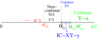
Figure 1: The phase diagram of Eq.2 when $\alpha=\beta^{+}$. The state at $\alpha=\beta=\pi/2$ is just an AFM state in $\tilde{\tilde{SU}}(2)$ basis. When $\alpha_{in}<\alpha<\pi/2$, there is a gap opening in the collinear Y-x phase generated by the order from quantum disorder (OFQD) mechanism. There is a second order quantum Lifshitz transition (QLT) at $\alpha=\alpha_{in}$ with the dynamic exponent $z=1$, from the Y-x phase to the coplanar IC-XY-y phase notation , then a second one to the C- non-coplanar $3\times 3$ SkX phase at $\alpha=\alpha_{33}$. The relevant numbers are $\alpha^{0}_{in}\sim 0.3611\pi,\alpha_{in}\sim 0.3526\pi,\alpha_{33}\sim 0.3402\pi,\alpha^{-}_{33}\sim 0.295\pi$ and the ordering wavevector in the IC-XY-y is $\pi-q^{0}_{y}$ with $q_{ic}\sim 0.18\pi<q^{0}_{y}<0.24\pi$. When $\alpha=\beta^{-}$. All the phases become their corresponding imaging phases related by the $[C_{4}\times C_{4}]_{D}$ transformation except the $3\times 3$ SkX phase is its own image. So the two corresponding imaging phases can coexist with any ratio along $\alpha=\beta$.

2. The order from quantum disorders: selection of the quantum ground state: It was shown the $2\times 1$ ( Y-x ) staterh ; notation is the exact quantum ground state along the anisotropic line $(\alpha=\pi/2,\alpha<\beta)$. Now we investigate the physics along the diagonal line $\alpha=\beta$ near the Abelian point $\alpha=\beta=\pi/2$. At the classical level, the $2\times 1$ Y-x state $S^{y}=(-1)^{x}$ ( Fig.2a) is degenerate with the $1\times 2$ X-y state $S^{x}=(-1)^{y}$. In fact, due to a spurious $U(1)$ symmetry, there is a family of states called $2\times 2$ vortex states in Fig.2c: $\mathbf{S}_{i}=((-1)^{i_{y}}\cos\phi,(-1)^{i_{x}}\sin\phi,0)$ which are degenerate at the classical level. The order from quantum disorder (OFQD) mechanism is needed to find the unique quantum ground state upto the $[C_{4}\times C_{4}]_{D}$ symmetry in this regime. After making suitable rotations to align the spin quantization axis along the Z axis, we introduce 4 HP bosons $a,b,c,d$ corresponding to the 4 sublattice structure $A,B,C,D$ shown in Fig.2c to perform a systematic $1/S$ spin wave expansion swgap ; sw1 ; japan for a generic $(\alpha,\beta)$: $H=E_{0}+2JS\Big{[}H_{2}+\Big{(}\frac{1}{\sqrt{S}}\Big{)}H_{3}+\Big{(}\frac{1}{\sqrt{S}}\Big{)}^{2}H_{4}+\cdots\Big{]}$ where $E_{0}=-2NJS^{2}(1-\cos 2\alpha\sin^{2}\phi-\cos 2\beta\cos^{2}\phi)$ is the classical ground state energy, $H_{n}$ denotes the $n$-th polynomial of the boson operators. $H_{2}$ can be diagonized by a unitary transformation, followed by a Bogoliubov transformation as:

$$H_{2}=E_{2}+2\sum_{n,k}\omega_{n}(k)\alpha_{n,k}^{\dagger}\alpha_{n,k}$$ (3)

where $n=1,2,3,4$ is the sum over the 4 branches ( due to the 4 sublattice $A,B,C,D$ in Fig.2c ) of spin wave spectrum in the Reduced BZ $-\pi/2<k_{x},k_{y}<\pi/2$ and $E_{2}(\phi)=\sum_{k,n}[\omega_{n}(k)-(1-\cos 2\alpha\sin^{2}\phi-\cos 2\beta\cos^{2}\phi)/2]$ is the $1/S$ quantum correction to the ground-state energy.

We first look at $E_{0}$ near the Abelian point $\alpha=\beta=\pi/2$. If $\alpha>\beta$, it picks the Y-x state rh with $\phi=\pi/2$. If $\alpha<\beta$, it picks the X-y state with $\phi=0$. Setting $\alpha=\beta$, $E_{0}=-2NJS^{2}(1-\cos 2\alpha)$ becomes $\phi$ independent, indicating the classical degenerate family of states characterized by the angle $\phi$ along the whole diagonal line $\alpha=\beta$. Fortunately, the quantum correction $E_{2}(\phi)=\sum_{k,n}[\omega_{n}(k,\phi)-\sin^{2}\alpha]$ does depend on $\phi$. As shown in Fig.3a, $E_{2}(\phi)$ reach its minimum at $\phi=0$ ( X-y state ) or $\phi=\pi/2$ ( Y-x state) which is related to each other by the $[C_{4}\times C_{4}]_{D}$ symmetry. Expanding $E_{2}(\phi)$ around one of its minima $\phi=0$:

$$E_{2}(\phi)=E_{2}^{0}+\frac{1}{2}B\phi^{2}+\kappa\phi^{4}+\cdots$$ (4)

where one can identify the coefficient $B(\alpha)$ plotted in the Fig.3b. The OFQD selection of the Y-x or X-y state at $\alpha=\beta$ shows that there is a direct first order transition from the Y-x state to the X-y state, so at $\alpha=\beta$, there is any mixture of the Y-x and X-y state in Fig.1.

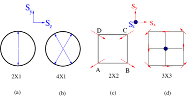
Figure 2: The Collinear, spiral, vortex and non-coplanar states in Fig.1. (a) The $2\times 1$ ( Y-x ) state $S^{y}=(-1)^{x}$ (b) The spin direction at the lattice sites $x=1,2,3,4$ of the $4\times 1$ spiral state. The inset shows the spin axis for the collinear and spiral states. (c) The classically degenerate family of ( 2 in , 2 out ) $2\times 2$ vortex state. (d) The $3\times 3$ non-coplanar skyrmion crystal ( SkX ) state with non-vanishing skyrmion density $\vec{S}_{i}\cdot\vec{S}_{j}\times\vec{S}_{k}\neq 0$ happens near $\alpha=\beta=\pi/3$ which is the most frustrated regime in the Wilson loop rh . The inset shows the spin axis for the $2\times 2$ vortex and $3\times 3$ SkX states.

Taking the Y-x state as the ground state, plugging $\phi=\pi/2$ into Eq.3, we find it supports the C_π magnons rh ; notation at $\mathbf{k}=(0,\pi)+\mathbf{q}$. They condense along the diagonal line $\arccos(1/\sqrt{6})\leq\alpha\leq\pi/2$ with the gapless relativistic dispersion:

$$\omega_{-0}(q)=\sqrt{v_{x}^{2}q_{x}^{2}+v_{y}^{2}q_{y}^{2}}$$ (5)

where $v_{x}=\cos(\alpha)/2,~{}v_{y}=\cos(\alpha)\sqrt{1-6\cos^{2}(\alpha)}/2$. Obviously, both velocities vanish at the Abelian point $\alpha=\beta=\pi/2$ dictated by the hidden $\tilde{\tilde{SU}}(2)$ symmetry. Moving away from the Abelian point, $v_{x}$ keeps increasing, but $v_{y}$ increases first, reaches a maximum, then decreases, vanishes at $\alpha^{0}_{ic}=arccos(1/\sqrt{6})\sim 0.36614\pi$, indicating a possible quantum Lifshitz transition (QLT). As to be shown below, the gapless magnon mode in Eq.5 is just a spurious Goldstone mode due to the spontaneous breaking of the spurious $U(1)$ symmetry.

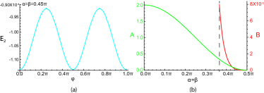
Figure 3: The order from the quantum disorder (OFQD) and the gap opening on the spurious gapless mode in the Y-x state in Fig.1. (a) The quantum correction $E_{2}(\phi)$ to the ground-state energy picks up Y-x at $\phi=0$ or X-y at $\phi=\pi/2$ as the ground state which is related to each other by the $[C_{4}\times C_{4}]_{D}$ symmetry. (b) The classical coefficient $A(\alpha)/J$ labeled by the left axis ( the green line on the left ) and the quantum one $B(\alpha)/J$ labeled by the right axis ( the red line on the right ). Both vanish at the Abelian point $\alpha=\beta=\pi/2$ as $\sim(\pi/2-\alpha)^{2}$ and are monotonically increasing function when moving away from the Abelian point. The Dashed line is located at $\alpha^{0}_{in}\sim 0.3661\pi$ where the Y-x state becomes unstable at the linear spin wave order. After incorporating the gap opening, the $\alpha^{0}_{in}$ is shifted to a smaller value $\alpha_{in}\sim 0.3526\pi$. The gap $\Delta_{B}$ in Eq.7 keeps increasing when moving away from the Abelian point $\alpha=\beta=\pi/2$.

3. Order from quantum disorder (OFQD): the gap opening and the spectrum: By using the spin coherent state path integral formulation aue ; sachdev ; swgap , we will evaluate the gap at the minimum $(0,\pi)$ of the $C_{\pi}$ magnons in the $\tilde{\tilde{SU}}(2)$ basis rh . A general uniform state at $\vec{q}=0$ in the $\tilde{\tilde{SU}}(2)$ basis can be taken as a Ferromagnetic (FM) state with the polar angle $(\theta,\phi)$. After transforming back to the original basis by using $\tilde{\tilde{S}}_{1}=R_{z}(\pi)S_{1},~{}\tilde{\tilde{S}}_{2}=R_{y}(\pi)S_{2},\tilde{\tilde{S}}_{3}=R_{x}(\pi)S_{3},\tilde{\tilde{S}}_{4}=S_{4}$, it leads to a $2\times 2$ state characterized by the two angles $\theta$ and $\phi$. Along the diagonal line, its classical energy becomes $H_{0}=J[-2\sin^{2}\alpha-2\cos^{2}\alpha\sin^{2}\theta]$ which is, as expected, $\phi$ in-dependent. Any deviation from the Abelian point picks up the XY plane with $\theta=\pi/2$. So it reduces to the $2\times 2$ vortex state shown in Fig.2c. Expanding around the minimum $H_{0}=J[-2\sin^{2}\alpha+2\cos^{2}\alpha(\theta-\frac{\pi}{2})^{2}+\cdots]$ gives the stiffness $A=2J\cos^{2}\alpha$ shown in Fig.3b. Using the spin coherent state analysis, we can write down the quantum spin action at $\vec{q}=0$:

$${\cal L}(\vec{q}=0)=iS\cos\theta\partial_{\tau}\phi+\frac{1}{2}S^{2}A(\theta-\pi/2)^{2}+\frac{1}{2}SB\phi^{2}$$ (6)

where we put back the spin $S$, the first term is the spin Berry phase term, $A\sim(\pi/2-\alpha)^{2}$ and $B\sim(\pi/2-\alpha)^{2}$ are from the classical analysis and the OFQD analysis Eqn.4 respectively. Eqn.6 leads to the gap

$$\Delta_{B}=\sqrt{SAB}\propto\sqrt{S}$$ (7)

which is beyond any $1/S$ expansion, so non-perturbative. In fact, there are also corrections from the cubic $H_{3}$ and quartic $H_{4}$ terms in the spin wave expansion listed above Eqn.3, but they only contribute to order of $1$ which is subleading to the $\sqrt{S}$ order in the $1/S$ expansion swgap ; sw1 ; japan . As shown in Fig.3b, both $A$ and $B$ are monotonically increasing along the diagonal line, so the gap also increase. Plugging their values at $\alpha=\alpha^{0}_{in}=\arccos(1/\sqrt{6})$, Taking $A/J=1/3,B/J\approx 8\times 10^{-3}$ and $S=1/2$, we find the maximum gap near the quantum Lifshitz transition $\Delta_{B}/J\sim 0.036$.

In the SM1 SM , we develop a new systematic non-perturbative scheme to evaluate not only the mass gap Eq.7, but also the whole spectrum:

$$\omega_{-}(q_{x},q_{y})=\sqrt{\Delta^{2}_{B}+v_{x}^{2}q_{x}^{2}+v_{y}^{2}q_{y}^{2}+u^{2}q_{y}^{4}+\cdots}$$ (8)

where $v^{2}_{y}=a(\alpha^{0}_{in}-\alpha)$ changes sign at $\alpha=\alpha^{0}_{in}$. From the gap vanishing condition loff ( See also Eq.10 ) at the IC- wave-vectors $q_{ic}=\pm(\Delta_{B}/u)^{1/2}$, one can see the QLT is shifted to $\alpha_{ic}=\alpha^{0}_{in}-2u\Delta_{B}/a$. Plugging in the values of $\Delta_{B}$ and $u$, we find $q_{ic}\sim 0.18\pi$. The shift is so small that $\alpha_{ic}\sim 0.3526\pi$ remains larger than $\alpha_{33}\sim 0.3402\pi$ ( to be defined in Sec.5 ) shown in Fig.1. So there must be an IC- phase intervening between the Y-x state and the $3\times 3$ state when $\alpha_{33}<\alpha<\alpha_{ic}$ in Fig.1.

4. The Quantum Lifshitz transition (QLT) from the Y-x phase to IC-XY-y phase: Here we construct an effective action in terms of the pseudo-Goldstone mode $\phi$ to describe the quantum Lifshitz transition. This is a symmetry based phenomenological approach which is independent of the $1/S$ expansion in the previous sections. Inside the Y-x phase along the diagonal line $\alpha=\beta$, after integrating out the massive conjugate variable $\theta-\pi/2$, we reach the following effective GL action in the continuum limit consistent with all the symmetries of the microscopic Hamiltonian Eq.2

$${\cal L}_{Y-x}[\phi] = \frac{1}{2A}(\partial_{\tau}\phi)^{2}+v^{2}_{x}(\partial_{x}\phi)^{2}+v^{2}_{y}(\partial_{y}\phi)^{2}+u^{2}(\partial^{2}_{y}\phi)^{2}$$ (9)

$$+ \frac{1}{2}B\phi^{2}+\kappa\phi^{4}+\cdots$$

In general, it is difficult to evaluate the values of the phenomenological parameters in Eq.9. However, in the large $S$ limit and away from the QLT point, they can be evaluated by the microscopic calculations in the previous sections. Indeed, by contrasting Eq.9 with Eq.6,7,8, one can see $A$ is from a classical contribution, $B$ and $\kappa$ are the effective potential Eq.4 generated from the OFQD mechanism. Notably, the coefficient $v^{2}_{y}=a(\alpha-\alpha^{0}_{in})$ tuned by the SOC changes sign at $\alpha=\alpha^{0}_{in}$. These matches between the microscopic calculations in a large $S$ limit and the symmetry based effective action ensures the non-perturbative OFQD calculation in Sec.3 is indeed correct.

It is physically more transparent to re-write Eq.9 in the momentum space:

$${\cal L}[\phi]_{Y-x,D} = \phi(-\omega_{n},-q_{x},-q_{y})[\omega^{2}_{n}/A+v^{2}_{x}q^{2}_{x}+u^{2}(q^{2}_{y}-q^{2}_{ic})^{2}$$ (10)

$$+ \Delta]\phi(\omega_{n},q_{x},q_{y})+\kappa\phi^{4}+\cdots$$

where $\Delta=\Delta^{2}_{B}-\frac{a^{2}}{4u^{2}}(\alpha-\alpha^{0}_{in})^{2}$ is the tuning parameter of the QLT.

The spin can be expressed in terms of the order parameter $\phi$ when using the shift $\phi\rightarrow\phi+\pi/2$ and setting $\phi$ small.

$$\mathbf{S}_{i}\sim(-(-1)^{i_{y}}\phi,(-1)^{i_{x}},0)$$ (11)

So we conclude that when $\Delta>0$, $\langle\phi\rangle=0$, it is inside the Y-x phase. When $\Delta<0$, then

$$\langle\phi\rangle=P_{0}\cos(q_{ic}y+\phi_{0})$$ (12)

where $P_{0},\phi_{0}$ need to be fixed by the 4th order $\kappa$ term. Substituting it into Eq.11 shows that the system is in the IC-XY-y phase notation . The smallness of $\langle\phi\rangle$ justifies the expansion in Eq.4. The transition from the Y-x to the IC- state is a quantum Lifshitz transition with the dynamic exponent $z=1$. All the quantum critical scalings will be evaluated in unlong by $1/N$ expansion and $4-\epsilon$ expansion with $\epsilon=1$.

5. The $3\times 3$ non-coplanar SkX phase: Near $\alpha=\beta=\pi/3$, it is natural to take a $3\times 3$ ansatz: $S_{(i_{x},i_{y})}=S_{(i_{x}+3m,i_{y}+3n)}$ with $m,n\in\mathbb{Z}$. We estimate its classical ground-state energy by minimizing $E_{3\times 3}(\{\phi_{i},\theta_{i}\}_{0\leq i\leq 9})$ over its 18 variables. Along the diagonal line ($\alpha=\beta$), as long as $\alpha$ is not too small, the minimization of $E_{3\times 3}$ always leads to the $3\times 3$ SkX state which respects the $[C_{4}\times C_{4}]_{D}$ symmetry ( Fig.2d ). The total spin in the $3\times 3$ unit cell is $S_{\rm unit}=\sum_{i}S_{i}=(0,0,4\times 10^{-3})$ which has exact vanishing $S_{x},S_{y}$ components, but still a small non-vanishing $S_{z}$ component.

Comparing the classical ground energy of the $3\times 3$ SkX with that of the Y-x state $E_{Y-x}=-2J\sin^{2}\alpha$ leads to a putative first order transition between the two states at $\alpha_{33}\approx 0.340188\pi$ which is smaller than $\alpha_{ic}\sim 0.3526\pi$ ( Fig.1 ). So a putative direct first order transition between the Y-x state and the $3\times 3$ SkX splits into two second order QLTs with $z=1$ with the IC-XY-y phase intervening between them in Fig.1. When approaching $\alpha=\beta$ from the anisotropic line $(\alpha=\pi/2,\beta)$ from the right unlong , we find $\alpha=\alpha_{33}$ lies on the constant contour line of the C-IC magnons $(0,k^{0}_{y})$ at $k^{0}_{y}\sim\pi-0.24\pi$. So $0.18\pi<q^{0}_{y}<0.24\pi$ in the IC-XY-y phase $\alpha_{33}<\alpha<\alpha_{in}$ (Fig.1).

6. Possible experimental implications: The heating issue has been well under control in the weak coupling limit in recent cold atom experiments expk40 ; expk40zeeman ; 2dsocbec ; clock ; clock1 ; clock2 ; SDRb ; ben ; gong . So various exotic magnetic superfluid phenomena can be observed in the current cold atom experiments. However, it gets worse as the coupling increases. The RFHM Eq.2 can only be reached in the strong coupling limit. So the rich magnetic Mott phenomena discovered in this manuscript can be observed only after the heating issue can be resolved in the strong coupling limit. Now, we turn its qualitative applications in the strongly correlated 4d or 5d materials with strong SOC.

Naively, due to its microscopic bosonic nature, the RFHM Eq.2 may not be useful to describe the magnetism in various materials with SOC. However, the RFHM can be expanded rh as Heisenberg-Kitaev (or Compass)- Dzyaloshinskii-Moriya (DM) dm1 form:

$$H_{R}=\sum_{\langle ij\rangle}J_{H}\vec{S}_{i}\cdot\vec{S}_{j}+\sum_{\langle ij\rangle a}J_{K}S^{a}_{i}S^{a}_{j}+\sum_{\langle ij\rangle a}J_{D}\hat{a}\cdot\vec{S}_{i}\times\vec{S}_{j}$$ (13)

where $\hat{a}=\hat{x},\hat{y}$ and $J_{H}=\cos 2\alpha,J_{K}=2\sin^{2}\alpha,J_{D}=\sin 2\alpha$. One can estimate their separate numerical values near the in-commensurate phase ( IC-XY-y ) $\alpha=\alpha^{0}_{in}=\arccos\frac{1}{\sqrt{6}}$ in Fig.1: the Heisenberg term $J_{H}\sim-2/3$ is AFM, the Kitaev term $J_{K}\sim 5/3$ is FM, the DM term $J_{D}\sim\sqrt{5}/3$. So the model becomes a dominant FM Kitaev term plus a small AFM Heisenberg term and a small DM term. This is indeed the case in the so called 5d Kitaev materials such as $A_{2}IrO_{3}$ with $A=Na_{2},Li_{2}$ or more recent 4d materials $\alpha-RuCl_{3}$. So far, only a Zig-Zag phase or an IC- phase were observed experimentally kitaevlattice ; kitaevlattice1 , no quantum spin liquids kit ; kit123 have been found.

7. Discussions: It is instructive to contrast the Quantum phenomena achieved here by the analytic perturbative and non-perturbative methods with those results achieved by classical Monte-Carlo simulations in the two earlier works classdm1 ; classdm2 . The authors in classdm1 ; classdm2 did classical Monte-Carlo simulations using the representation Eq.13 on a small finite size system. These two numerical papers did not have the concepts of the frustrations due to the Rashba SOC. Ref.classdm1 found the classical $2\times 1$, $3\times 3$ SkX and $4\times 1$ states in Fig.1. It also found a Ferromagnetic (FM) state near the orgigin $\alpha=\beta=0$. Ref.classdm2 found the classical $2\times 2$ vortex, $3\times 3$ SkX and $4\times 1$ states in Fig.1. Our work study the quantum effects on the RFHM Eq.2 analytically . In Sec.2, we found the $2\times 2$ vortex is classically degenerate with the Y-x and X-y state, but the ” order form quantum disorder” (OFQD) mechanism picks up either Y-x and X-y state as the quantum ground state. In Sec.3, we also evaluated the excitation spectrums corrected by the mechanism. This anlysis also leads to the instability of the Y-x ( or X-y ) state to the IC-SkX phase. In Sec.4, we constructed an effective action to describe the quantum Lifshitz transition (QLT) with the dynamic exponent $z=1$ in Fig.1 and also identify the spin-orbital structure of the IC-SkX phase. Of course, it would be impossible to detect the quantum IC-SkX phase by any classical Monte-Carlo simualations at any finite size system, let alone to study the QLT. Only by the controlled, non-perturabative analytical calculations, one can show there must be an in-commensurate phase intervening between the collinear Y-x phase and the non-coplanar $3\times 3$ SkX phase. Of course, the quantum model Eq.2 presents very serious sign problem to quantum Monte-Carlo simulation. So the classical classical Monte-Carlo simualations used in classdm1 ; classdm2 can not be extended to study the novel quantum and topological phenomena address in this work.

As alerted above, the second term in Eq.13 is a quantum compass model in a square lattice instead of the Kitaev model in a honeycomb lattice. In order to have quantitative impacts on the 3d or 4d Kitaev materials kitaevlattice ; kitaevlattice1 , it is important to extend the results achieved here in a square lattice to a honeycomb lattice with 3 SOC parameters $\alpha,\beta,\gamma$.

We thank Wei Ku for the hospitality during our visit at T D Lee institute. We acknowledge AFOSR FA9550-16-1-0412 for supports.

References

- (1) A. Auerbach, Interacting electrons and quantum magnetism, (Springer Science & Business Media, 1994).
- (2) S. Sachdev, Quantum Phase transitions, (2nd edition, Cambridge University Press, 2011).
- (3) L. Savary and L. Balents, Quantum Spin liquids, arXiv:1601.03742 (2016).
- (4) C. Broholm, R. J. Cava, S. A. Kivelson, D. G. Nocera, M. R. Norman, T. Senthil, Quantum spin liquids, Science 17 Jan 2020: Vol. 367, Issue 6475, eaay0668, DOI: 10.1126/science.aay0668
- (5) A. Kitaev, Anyons in an exactly solved model and beyond, Ann. Phys. 321, 2 (2006). In the context of the present paper, the difference between honeycomb and a square lattice is not essential.
- (6) Erhai Zhao and W. Vincent Liu, Orbital Order in Mott Insulators of Spinless -Band Fermions, Phys. Rev. Lett. 100, 160403 (2008).
- (7) Congjun Wu, Orbital Ordering and Frustration of -Band Mott Insulators, Phys. Rev. Lett. 100, 200406 (2008).
- (8) Haiyuan Zou, Bo Liu, Erhai Zhao, W. Vincent Liu, A continuum of compass spin models on the honeycomb lattice, New J. Phys. 18 053040 (2016).
- (9) Ji Chaloupka, George Jackeli, and Giniyat Khaliullin, Zigzag Magnetic Order in the Iridium Oxide Na2IrO3, Phys. Rev. Lett. 110, 097204 (2013).
- (10) Y. A. Bychkov and E.I. Rashba, Oscillatory effects and the magnetic susceptibility of carriers in inversion layers, J. Phys. C 17, 6039 (1984).
- (11) Jinwu Ye, Yong Baek Kim, A. J. Millis, B. I. Shraiman, P. Majumdar, and Z. Tesanovic, Berry phase theory of the Anomalous Hall Effect: Application to Colossal Magnetoresistance Manganites, Phys. Rev. Lett. 83, 3737 (1999)
- (12) Lev P. Gor’kov and Emmanuel I. Rashba, Superconducting 2D System with Lifted Spin Degeneracy: Mixed Singlet-Triplet State, Phys. Rev. Lett. 87, 037004 (2001).
- (13) T. Jungwirth, Qian Niu and A. H. MacDonald, Anomalous Hall Effect in Ferromagnetic Semiconductors, Phys. Rev. Lett. 88, 207208 (2004).
- (14) Jairo Sinova, Dimitrie Culcer, Q. Niu, N. A. Sinitsyn, T. Jungwirth, and A. H. MacDonald, Universal intrinsic spin Hall effect, Phys. Rev. Lett. 92, 126603 (2004).
- (15) Wang Yao and Qian Niu, Berry Phase Effect on the Exciton Transport and on the Exciton Bose-Einstein Condensate, Phys. Rev. Lett. 101, 106401 (2008).
- (16) Naoto Nagaosa, Jairo Sinova, Shigeki Onoda, A. H. MacDonald, and N. P. Ong, Anomalous Hall effect, Rev. Mod. Phys. 82, 1539 (2010).
- (17) Jairo Sinova, Sergio O. Valenzuela, J. Wunderlich, C.?H. Back, and T. Jungwirth, Spin Hall effects, Rev. Mod. Phys. 87, 1213 (2015).
- (18) Lianghui Huang, et.al, Experimental realization of a two-dimensional synthetic spin-orbit coupling in ultracold Fermi gases, Nature Physics 12, 540 (2016).
- (19) Zengming Meng, et.al, Experimental observation of topological band gap opening in ultracold Fermi gases with two-dimensional spin-orbit coupling, arXiv:1511.08492.
- (20) Zhan Wu, et.al, Realization of Two-Dimensional Spin-orbit Coupling for Bose-Einstein Condensates, Science 354, 83 (2016).
- (21) Zong-Yao Wang et.al, Realization of an ideal Weyl semimetal band in a quantum gas with 3D spin-orbit coupling, Science 372, 271 (2021).
- (22) Michael L. Wall, et.al, Synthetic Spin-Orbit Coupling in an Optical Lattice Clock, Phys. Rev. Lett. 116, 035301 (2016).
- (23) L. F. Livi, G. Cappellini, M. Diem, L. Franchi, C. Clivati, M. Frittelli, F. Levi, D. Calonico, J. Catani, M. Inguscio, L. Fallani, Synthetic dimensions and spin-orbit coupling with an optical clock transition, Phys. Rev. Lett. 117, 220401 (2016).
- (24) S. Kolkowitz, S.L. Bromley, T. Bothwell, M.L. Wall, G.E. Marti, A.P. Koller, X. Zhang, A.M. Rey, J. Ye, Spin-orbit coupled fermions in an optical lattice clock, arXiv:1608.03854.
- (25) Fangzhao Alex An, Eric J. Meier, Bryce Gadway, Direct observation of chiral currents and magnetic reflection in atomic flux lattices, arXiv:1609.09467.
- (26) Nathaniel Q. Burdick, Yijun Tang, and Benjamin L. Lev, Long-Lived Spin-Orbit-Coupled Degenerate Dipolar Fermi Gas, Phys. Rev. X 6, 031022 (2016).
- (27) Zi Cai, Xiangfa Zhou, and Congjun Wu, Magnetic phases of bosons with synthetic spin-orbit coupling in optical lattices, Phys. Rev. A 85, 061605 (2012).
- (28) J. Radić, A. Di Ciolo, K. Sun, and V. Galitski, Exotic Quantum Spin Models in Spin-Orbit-Coupled Mott Insulators, Phys. Rev. Lett. 109, 085303 (2012);
- (29) W. S. Cole, S. Zhang, A. Paramekanti, and N. Trivedi, Bose-Hubbard Models with Synthetic Spin-Orbit Coupling: Mott Insulators, Spin Textures, and Superfluidity, Phys. Rev. Lett. 109, 085302 (2012).
- (30) Fadi Sun, Jinwu Ye, Wu-Ming Liu, Quantum magnetism of spinor bosons in optical lattices with synthetic non-Abelian gauge fields, Phys. Rev. A 92, 043609 (2015).
- (31) Fadi Sun and Jinwu Ye, Two classes of organization principle: quantum/topological phase transitions meet complete/in-complete devil staircases and their experimental realizations, arXiv:1603.00451, in preparation.
- (32) Here we still use the same notation used in rh . In the Y- called Y-x state, the first letter indicates the spin polarization, the second letter indicates the orbital order. Along the anisotropic line , it supports three kinds of magnons C0, IC and Cπ with their minimum at and respectively. The IC-XY-y phase means IC- in the spin XY plane with the IC- momentum along the y axis.
- (33) Murthy, G., Arovas, D. & Auerbach, A. Superfluids and supersolids on frustrated two-dimensional lattices. Phys. Rev. B 55, 3104 (1997).
- (34) R. T. Scalettar, G. G. Batrouni, A. P. Kampf, and G. T. Zimanyi, Simultaneous diagonal and off-diagonal order in the Bose-Hubbard Hamiltonian, Phys. Rev. B 51, 8467 (1995).
- (35) Jun-ichi Igarashi, 1/S expansion for thermodynamic quantities in a two-dimensional Heisenberg antiferromagnet at zero temperature, Phys. Rev. B 46, 10763-10771 (1992); Jun-ichi Igarashi and Tatsuya Nagao, -expansion study of spin waves in a two-dimensional Heisenberg antiferromagnet, Phys. Rev. B 72, 014403 (2005).
- (36) See the supplementary material for the derivation of the complete excitation spectrum Eq.8 due to the OFQD phenomena.
- (37) Longhua Jiang and Jinwu Ye, Lattice structures of Larkin-Ovchinnikov-Fulde-Ferrell (LOFF) state, Phys. Rev. B 76, 184104 (2007).
- (38) Gong, M. et al. Dzyaloshinskii-Moriya Interaction and Spiral Order in Spin-orbit Coupled Optical Lattices. Sci. Rep. 5, 10050, 2015.
- (39) I. Dzyaloshinskii, J. Phys. Chem. Solids 4, 241 (1958); T. Moriya, Phys. Rev. 120, 91 (1960).
- (40) A. Biffin, et.al, Noncoplanar and Counterrotating Incommensurate Magnetic Order Stabilized by Kitaev Interactions in Li2IrO3, Phys. Rev. Lett. 113, 197201 (2014).
- (41) A. Biffin, et. al , Unconventional magnetic order on the hyperhoneycomb Kitaev lattice in Li2IrO3: Full solution via magnetic resonant x-ray diffraction, Phys. Rev. B 90, 205116 (2014).