Supervised Learning based Sparse Channel Estimation for RIS aided Communications

Abstract

An reconfigurable intelligent surface (RIS) can be used to establish line-of-sight (LoS) communication when the direct path is compromised, which is a common occurrence in a millimeter wave (mmWave) network. In this paper, we focus on the uplink channel estimation of a such network. We formulate this as a sparse signal recovery problem, by discretizing the angle of arrivals (AoAs) at the base station (BS). On-grid and off-grid AoAs are considered separately. In the on-grid case, we propose an algorithm to estimate the direct and RIS channels. Neural networks trained based on supervised learning is used to estimate the residual angles in the off-grid case, and the AoAs in both cases. Numerical results show the performance gains of the proposed algorithms in both cases.

Index Terms—  Intelligent reflecting surfaces, mmWave communications, channel estimation, sparse recovery, supervised learning.

1 Introduction

Reconfigurable intelligent surfaces (RISs) have resulted a new wave of research towards the reconfigurability of the wireless propagation environment, with software controlled scattering of the incoming waves. The phase shifts of the individual elements can be configured smartly to achieve favourable conditions, for a given application. The passive operation and lower cost of these devices attracts more and more applications [1, 2, 3].

The smart reconfigurability of an RIS depends on the availability of channel state information (CSI). An RIS consists of a large number of passive reconfigurable elements in general, which results in a large number of propagation paths in addition to the direct path. Hence, the channel estimation for RIS aided systems is challenging. Grouping of reconfigurable elements [4], and relying on angle of arrival (AoA) of the line-of-sight (LoS) base station (BS)-RIS channel and the angle of departure (AoD) of the LoS RIS-User [5] for passive beamforming has been used to overcome some of these challenges.

Channel estimation for RISs requires the design of activation patterns for the RIS elements. The impact of RIS activation pattern on the channel estimation performance is investigated in [6], where an optimal codebook is proposed based on a minimum variance unbiased estimator. The angular domain sparsity in millimetre wave (mmWave) channels can be exploited to reduce the dimensionality of the parameter space, which results in a reduced pilot overhead. A sparse representation of the concatenated BS-IRS-user (cascaded) channel is derived in [7], which convert channel estimation into a sparse signal recovery problem. The double-structured sparsity of the angular cascaded channels is leveraged in [8] to propose a double-structured orthogonal matching pursuit (DS-OMP) based cascaded channel estimation scheme.

Compared to optimization based approaches in traditional communication algorithms, neural networks (NNs) provides the ability to learn complex patterns from data itself. This is beneficial in situations where the development of an algorithm is difficult due to the complexity of the problem. Supervised learning is applied for training when a labelled data set is available, where the outputs corresponds to the inputs are tabulated. Some applications of NNs related to channel estimation can be found in [9, 10, 11, 12].

A major use case of RIS is to establish LoS through the reflected path when the user does not have LoS with the BS, but with the RIS. In this case, the joint channel from user to BS contains a specular component dominated by the reflected LoS link through RIS and, a scattering component from the direct Non-LoS (NLoS) link. A novel channel model for a similar scenario is proposed in [13], where a compact expression for the channel distribution is derived.

In our work we consider the uplink of a mmWave network, where an RIS is used to assist the communication. We focus on utilizing an RIS in a scenario where the user lacks LoS with the BS. Based on this model, we develop a compact representation for the RIS channel. An angular domain sparse channel model is considered by discretizing the AoAs. The channel estimation problem is formulated step by step for the case where AoAs lie exactly on the discrete grid (on-grid), and the case where AoAs can take any discrete value deviating from discrete grid (off-grid). A sparse estimation method is proposed for the on-grid case, based on OMP, and a NN based approach is used for comparison. In the off-grid case, a two-step procedure is used to perform channel estimation, where first, on-grid AoAs are estimated using a NN and then off-grid AoAs are calculated by predicting the residuals using another NN.

2 System Model

We consider the uplink channel estimation of a mmWave network consisting of a single antenna user and a BS with $M$ antennas. An RIS with $N$ reflecting elements is used to assist the communication, while the reflecting elements are arranged in $G$ groups to reduce the training overhead [1]. As illustrated in Fig. 1, the channel consists of a direct link which is non-line-of sight (NLoS), and a link through RIS which consist of line-of-sight (LoS) components. Let $\bm{H}_{r}\in\mathbb{C}^{M\times N}$ be the channel between RIS and BS, $\bm{h}_{v}\in\mathbb{C}^{N}$ be the channel between user and RIS, and $\bm{h}_{d}\in\mathbb{C}^{M}$ be the direct channel between user and BS. Let $\bm{\Theta}=\text{diag}(\bm{v})$ denote the reflection matrix of the RIS, where $\bm{v}=[e^{j\alpha_{1}},e^{j\alpha_{2}},...,e^{j\alpha_{N}}]^{T}$ with $\alpha_{n}$ being the phase shift of the $n$th reflecting element.

Fig. 1: Illustration of the system model.

Since, user-RIS and RIS-BS links are LoS, we can express them as follows, in terms of the array responses of the RIS and BS,

$$\bm{h}_{v}=c_{v}\bm{a}_{RIS}(\theta_{R}^{RIS}),$$ (1)

and

$$\bm{H}_{r}=c_{r}\bm{a}_{BS}(\theta_{R}^{BS})\left[\bm{a}_{RIS}(\theta_{T}^{RIS})\right]^{H},$$ (2)

where $\bm{a}_{RIS}()$, $\bm{a}_{BS}()$ are the array responses of BS and RIS, and $\theta_{R}^{RIS}$, $\theta_{R}^{BS}$ and $\theta_{T}^{RIS}$ are the AoA at RIS, AoA at the BS and AoD at the RIS respectively. Here, $c_{r}$ and $c_{v}$ are the complex path gains of the links. A planar geometry is assumed in the derivations. Now, the effective channel through RIS can be expressed as,

$$\begin{split}\bm{g}&=\bm{H}_{r}\bm{\Theta}\bm{h}_{v}\\ &=c_{r}\bm{a}_{BS}(\theta_{R}^{BS})\left[\bm{a}_{RIS}(\theta_{T}^{RIS})\right]^{H}c_{v}\bm{\Theta}\bm{a}_{RIS}(\theta_{R}^{RIS})\\ &=\bm{a}_{BS}(\theta_{R}^{BS})\left(\sum_{n=1}^{N}\gamma_{n}^{*}e^{j\alpha_{n}}\right)\\ &=\bm{a}_{BS}(\theta_{R}^{BS})\bm{\gamma}^{H}\bm{v},\end{split}$$ (3)

where $\bm{\gamma}=[\gamma_{1},\gamma_{2},...,\gamma_{N}]^{T}$ with $\gamma_{n}=c_{r}c_{v}\left[a_{RIS,n}(\theta_{T}^{RIS})\right]$ $a_{RIS,n}(\theta_{R}^{RIS})^{*}$.

3 Problem Formulation

3.1 On-Grid AoAs

We assume a mmWave scattering channel model for the direct channel. The time is divided into frames, and in each frame, the user transmits several pilot symbols for channel estimation. The pilot symbols are generated by changing the phase shifts of the RIS by going through the entries of a predefined codebook [6]. The effective channel $\bm{h}_{t,i}\in\mathbb{C}^{M}$ between the user and BS at the $i$th symbol of the $t$th frame is,

$$\begin{split}\bm{h}_{t,i}&=\bm{g}_{t,i}+\sum_{q=1}^{S}\beta_{t,q}\bm{a}_{R}(\theta_{t,q})\\ &=\bm{a}_{R}(\theta_{t,0})\bm{\gamma}_{t}^{H}\bm{v}_{t,i}+\sum_{q=1}^{S}\beta_{t,q}\bm{a}_{R}(\theta_{t,q}),\end{split}$$ (4)

where $\bm{a}_{R}(\theta_{t,q})\in\mathbb{C}^{M}$ is the steering vector at the BS with $\theta_{t,q}$ being the AoA at the BS for the $q$th path, and $\beta_{t,q}$ is the complex path gain. Here, $\bm{g}_{t,i}$ is channel through RIS, $\theta_{t,0}$ corresponds to the AoA for the RIS-BS path and $\bm{g}_{t,i}=\bm{\gamma}_{t}^{H}\bm{v}_{t,i}$, where $\bm{\gamma}_{t}$ is the complex path gain vector through RIS reflecting elements defined above.

Let us consider an angular domain channel representation, where the angle of arrival is assumed to be from a grid of $K$ AoAs. A dictionary $\bm{A}_{R}\in\mathbb{C}^{M\times(K+1)}$ is formed by the steering vectors of the grid points $\tilde{\theta}_{k},\text{ for }k=0,1,\cdots,K$,

$$\bm{A}_{R}=\begin{bmatrix}\bm{a}_{R}(\tilde{\theta}_{0})&\bm{a}_{R}(\tilde{\theta}_{1})&\cdots&\bm{a}_{R}(\tilde{\theta}_{K})\end{bmatrix},$$ (5)

where $\tilde{\theta}_{0}$ corresponds to the AoA for RIS-BS link. Now we can write the channel vector as follows,

$$\bm{h}_{t,i}=\bm{A}_{R}\left(\bm{z}^{\prime}\bm{\gamma}_{t}^{H}\bm{v}_{t,i}+\bar{\bm{z}}_{t}\right),$$ (6)

where $\bar{\bm{z}}_{t}\in\mathbb{C}^{K}$ is the sparse complex channel gain vector for the NLoS path, and $\bm{z}^{\prime}$ is an all zeros vector except the first entry. The received signal at the $i$th time slot of the $t$th frame is,

$$\bm{y}_{t,i}=\bm{A}_{R}\left(\bm{z}^{\prime}\bm{\gamma}_{t}^{H}\bm{v}_{t,i}+\bar{\bm{z}}_{t}\right)x_{i}+\bm{n}_{t,i},$$ (7)

where $\bm{n}_{t,i}=[n_{t,i,1},n_{t,i,2},\cdots,n_{t,i,M}]$ is the additive white Gaussian noise (AWGN) added at the BS antenna, with $n_{t,i,j}\sim\mathcal{CN}(0,N_{0})$. For simplicity assume $x_{i}=1$. We observe the received signals while changing the phase shifts at the RIS for $L$ time slots. Let us also assume the channel parameters are not changing during this period. However, the complex channel gain through RIS changes depending on the phase shift configuration. Let $\bm{Q}_{t}=\bm{z}^{\prime}\bm{\gamma}_{t}^{H}$, and we can see that $\bm{Q}\in\mathbb{C}^{K\times N}$ is a sparse matrix. Now we can write the received signal as,

$$\bm{y}_{t,i}=\bm{A}_{R}(\bm{Q}_{t}\bm{v}_{t,i}+\bar{\bm{z}}_{t})+\bm{n}_{t,i}.$$ (8)

We can see that $\bm{A}_{R}\bm{Q}_{t}$ and $\bm{A}_{R}\bar{\bm{z}}_{t}$ corresponds to $\bm{\Phi}_{t}$ and $\bm{h}_{d,t}$. For convenience we drop the frame index. Let $\bm{Y}=\begin{bmatrix}\bm{y}_{1}&\bm{y}_{2}&\cdots&\bm{y}_{L}\end{bmatrix}$, $\bm{V}=\begin{bmatrix}\bm{v}_{1}&\bm{v}_{2}&\cdots&\bm{v}_{L}\end{bmatrix}$ and $\bm{N}=\begin{bmatrix}\bm{n}_{1}&\bm{n}_{2}&\cdots&\bm{n}_{L}\end{bmatrix}$. Therefore, we can write the following matrix equation,

$$\bm{Y}=\bm{A}_{R}\left(\bm{Q}\bm{V}+\bar{\bm{z}}\bm{\mathbf{1}}^{T}\right)+\bm{N}$$ (9)

We can express this in a compact notation by defining $\tilde{\bm{Q}}=\begin{bmatrix}\bar{\bm{z}}&\bm{Q}\end{bmatrix}$ and $\tilde{\bm{V}}=\begin{bmatrix}\bar{\bm{\mathbf{1}}}&\bm{V}\end{bmatrix}$. Now the Equation (9) can be written as,

$$\bm{Y}=\bm{A}_{R}\tilde{\bm{Q}}\tilde{\bm{V}}+\bm{N}.$$ (10)

3.2 Off-Grid AoAs

Although we have assumed on-grid AoAs, this is not the case in general. Therefore, in this section we modify the problem by relaxing on-grid AoA constraints. We introduce the residual AoA vector $\bm{\delta}=\begin{bmatrix}\delta_{0}&\delta_{1}&\cdots&\delta_{K}\end{bmatrix}$ such that $\delta_{k}=\begin{cases}\theta_{q}-\tilde{\theta}_{k_{q}},&q=k_{q}\text{, for }q=0,1,\cdots,S\text{, and }k\neq 0\\ 0,&\text{otherwise},\end{cases}$
where $k_{q}$ is the index of the grid point closest to the AoA of the $q$th path, and $\theta_{q}$, $\tilde{\theta}_{k_{q}}$ being the true AoA of the $q$th path and AoA value of the $k_{q}$th grid point respectively. Now the Equation (10) can be modified to include the new BS array response dictionary that depends on $\bm{\delta}$ as $\bm{A}_{R}(\bm{\delta})$, which is obtained by correcting the grid points with residual values. We can express the received signal by the following matrix equation,

$$\bm{Y}=\bm{A}_{R}(\bm{\delta})\tilde{\bm{Q}}\tilde{\bm{V}}+\bm{N}.$$ (11)

4 Algorithm Development

4.1 Algorithm Development for On-Grid AoAs

In this section we develop an algorithm to find the sparse solution of (10). In order to solve this problem we can use the known information regarding the sparsity of $\bm{Q}$ and $\bar{\bm{z}}$. We know that RIS act as single scarring element in our model, also it has a fixed location which can be perfectly known. On the other hand, $\bar{\bm{z}}$ should be $S$-sparse corresponding to the remaining scattering paths.

Let us consider the expansion of the matrix product $\tilde{\bm{Q}}\tilde{\bm{V}}=\sum_{j=0}^{N}\tilde{\bm{q}}_{j}\tilde{\bm{v}}_{j}^{T}$, where $\tilde{\bm{q}}_{j}$ is the $j$th row of $\tilde{\bm{Q}}$ and $\tilde{\bm{v}}_{j}$ is the $j$th column of $\tilde{\bm{V}}$. Assume we have chosen $\tilde{\bm{V}}$ such that $\tilde{\bm{v}}_{j}^{T}\tilde{\bm{v}}_{0}^{*}=0\text{, for all }j\neq 0$ (which is satisfied by the codebook in [6]). Multiplying equation (10) by $\tilde{\bm{v}}_{0}^{*}$, we can eliminate all the other terms except $\tilde{\bm{q}}_{0}\text{ }(=\bar{\bm{z}})$,

$$\begin{split}\bm{Y}\tilde{\bm{v}}_{0}^{*}&=\bm{A}_{r}\tilde{\bm{q}}_{0}\tilde{\bm{v}}_{0}^{T}\tilde{\bm{v}}_{0}^{*}+\bm{N}\tilde{\bm{v}}_{0}^{*}\\ \bm{y}^{\prime}&=\bm{A}_{r}\bar{\bm{z}}+\bm{n}^{\prime},\end{split}$$ (12)

where $\bm{y}^{\prime}=\frac{\bm{Y}\tilde{\bm{v}}_{0}^{*}}{\tilde{\bm{v}}_{0}^{T}\tilde{\bm{v}}_{0}^{*}}$ and $\bm{n}^{\prime}=\frac{\bm{N}\tilde{\bm{v}}_{0}^{*}}{\tilde{\bm{v}}_{0}^{T}\tilde{\bm{v}}_{0}^{*}}$. This corresponds to a sparse signal recovery problem and there exist many classical algorithms such as OMP, [14] which can be used to estimate $\bar{\bm{z}}$.

After finding $\bar{\bm{z}}$, we can focus on the estimation of RIS channel by essentially removing the effect of the direct path from the received signal. We can define the signal due to RIS path as follows,

$$\bm{Y}_{\text{RIS}}=\bm{Y}-\bm{A}_{r}\bar{\bm{z}}\tilde{\bm{v}}_{0}^{T}.$$ (13)

Since the AoA of the RIS-BS path is known, we can find $\bm{\gamma}$ by minimizing,

$$\|\bm{Y}_{\text{RIS}}-\bm{a}_{R}(\tilde{\theta}_{0})\bm{\gamma}^{H}\bm{V}\|_{2}^{2}.$$ (14)

The channel estimation procedure is expressed in Algorithm 1.

input : Received signal $\bm{Y}$, AoA grid $\bm{A}_{r}$ and augmented $\tilde{\bm{v}}_{0}$ and RIS phase shifts $\tilde{\bm{V}}$.

output : Estimated $\bm{\Phi}$ and $\bm{h}_{d}$

1 Find $\bar{\bm{z}}$ by solving (12) with OMP

2 Calculate $\bm{Y}_{\text{RIS}}$ by equation (13)

3 Calculate $\bm{\gamma}$ by minimizing (14)

4 $\bm{\Phi}=\bm{a}_{R}(\tilde{\theta}_{0})\bm{\gamma}^{H}$

5 $\bm{h}_{d}=\bm{A}_{R}\tilde{\bm{z}}$

Algorithm 1 On-grid channel estimation algorithm

4.2 Supervised Learning based Channel Estimation

The NN architecture used to calculate the AoAs is shown in Fig. 2, where it consists of several NNs. First, the on-grid AoAs are predicted using the top NN in the diagram. Stacked received signals over $L$ symbols is the input to this NN, and the residual AoAs are obtained at the output. The input feature is a complex vector, and we convert it to a real vector by stacking real and imaginary parts, which is fed to the network. At the output layer of this network sigmoid activation is used, which corresponds to the probability of a certain AoA grid point being present.

In the off-grid case, a collection of neural networks corresponding to each discrete grid point is used to predict the residual error in the AoA. These NNs are shown in the bottom part of the diagram. Each network has similar input as the on-grid AoA prediction network, while tanh activation is used at the output layer. In this case, first the on-grid point is identified by the top network and the residual error is predicted using the corresponding bottom network. Finally, the AoAs are calculated by correcting the error.

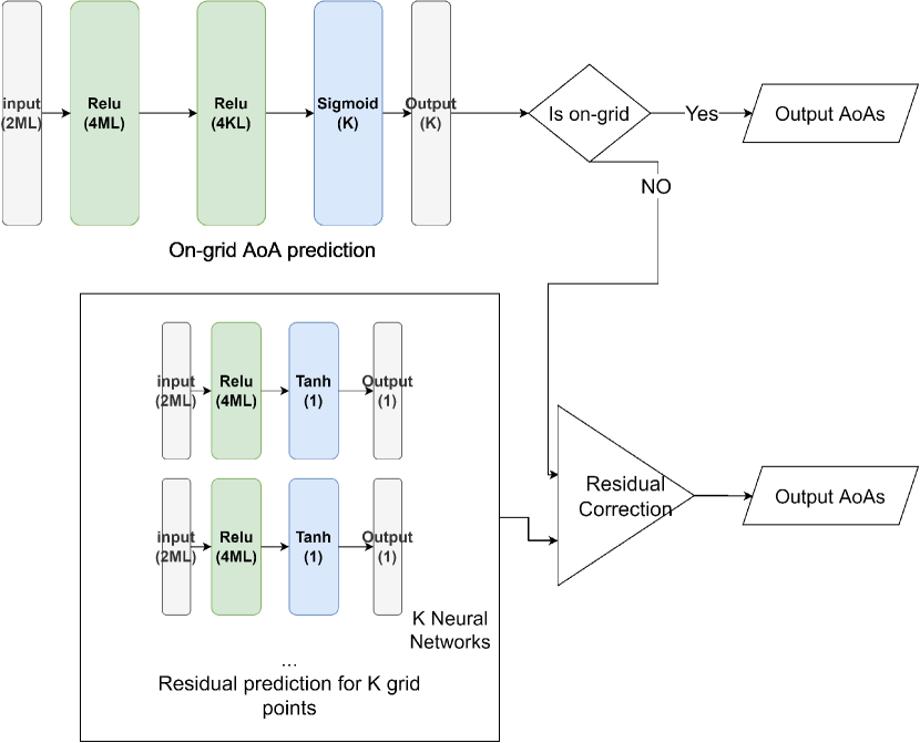
Fig. 2: NN architecture for residual AoA prediction.

5 Results

In this Section, we perform numerical simulations to evaluate the performance of the proposed algorithms. In all the simulations BS antenna is considered as a $16\times 1$ uniform linear array (ULA) oriented in the x-axis. The RIS is considered as a $16\times 16$ uniform planar array (UPA) oriented in the y-axis. The BS and RIS locations are fixed, and user locations are generated randomly. All the devices are assumed to be at the same elevation ($z=0$). The channel is generated based on a mmWave scattering model with random angles. The noise level has been set to -110 dBm and number of discrete AoA grid points ($K$) is set to $32$.

First, channel estimation with on-grid angles is simulated. Fig. 3 shows the plot of transmit power vs. normalized mean square error (NMSE). Results are generated using both Algorithm 1 and AoA prediction with the NN. Least squares (LS) estimation is also considered for comparison. Comparing the performance of direct channel estimation, we can see that Algorithm 1 outperforms LS at all power levels, while the performance gap also increases with increasing transmit power. The NN outperforms both LS and Algorithm 1, but the performance get saturated at high transmit power. RIS channel is estimated by following the rest of the steps of Algorithm 1 in both cases, and it outperforms LS estimation.

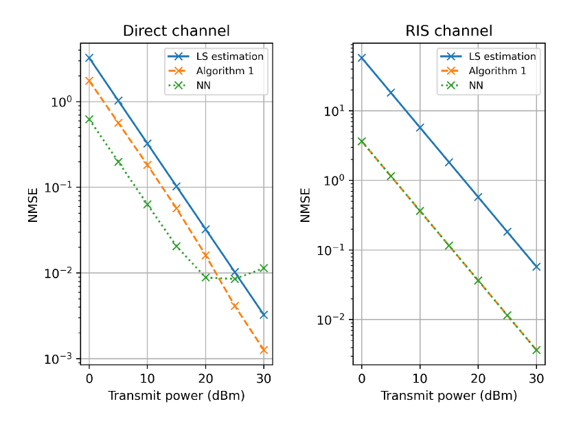
Fig. 3: Channel estimation with on-grid AoAs.

Next, off-grid AoAs are considered as shown in Fig. 4. Performance of Algorithm 1 is evaluated under both perfect and imperfect AoA values, where in the perfect case, residual errors of AoAs are assumed to be perfectly known. Although AoAs are off-grid, we see a similar performance to the on-grid case. The NN based solution outperforms both LS and algorithms. However, in the direct channel, a saturation of performance is seen at high transmit power as observed earlier in the on-grid case. A similar effect is seen for Algorithm 4 with imperfect AoAs. This is related to the increasing power leakage due to grid imperfections. As a result the NN struggles to predict the correct AoA point. RIS channel estimation shows a similar performance as the on-grid case.

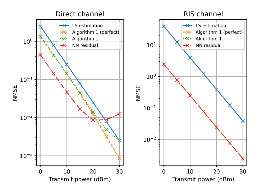
Fig. 4: Channel estimation with off-grid AoAs.

6 Conclusion

In this paper, we have considered the channel estimation of a mmWave network assisted by an RIS. We have formulated this as a sparse recovery problem by discretizing the AoAs. An algorithm was proposed to solve the on-grid case, along with NN based AoA prediction. In the off-grid case, another NN was used to predict the residual angles. Numerical simulations have shown that the proposed algorithm outperforms LS estimation. The NN network gives the best performance in both on-grid and off-grid cases, however, the performance gets saturated at high transmit power.

References

- [1] D. L. Dampahalage, K. B. S. Manosha, N. Rajatheva, and M. Latva-Aho, “Weighted-Sum-Rate Maximization for an Reconfigurable Intelligent Surface Aided Vehicular Network,” IEEE Open Journal of the Communications Society, vol. 2, pp. 687–703, 2021.
- [2] Z. Zhang and L. Dai, “Capacity Improvement in Wideband Reconfigurable Intelligent Surface-Aided Cell-Free Network,” in 2020 IEEE 21st International Workshop on Signal Processing Advances in Wireless Communications (SPAWC), 2020, pp. 1–5.
- [3] C. Pan, H. Ren, K. Wang, M. Elkashlan, A. Nallanathan, J.u Wang, and L. Hanzo, “Intelligent Reflecting Surface Aided MIMO Broadcasting for Simultaneous Wireless Information and Power Transfer,” IEEE Journal on Selected Areas in Communications, vol. 38, no. 8, pp. 1719–1734, 2020.
- [4] Y. Yang, B. Zheng, S. Zhang, and R. Zhang, “Intelligent Reflecting Surface Meets OFDM: Protocol Design and Rate Maximization,” IEEE Transactions on Communications, vol. 68, no. 7, pp. 4522–4535, 2020.
- [5] K. Ying, Z. Gao, S. Lyu, Y. Wu, H. Wang, and M.-S. Alouini, “GMD-Based Hybrid Beamforming for Large Reconfigurable Intelligent Surface Assisted Millimeter-Wave Massive MIMO,” IEEE Access, vol. 8, pp. 19530–19539, 2020.
- [6] T. L. Jensen and E. De Carvalho, “An Optimal Channel Estimation Scheme for Intelligent Reflecting Surfaces Based on a Minimum Variance Unbiased Estimator,” in ICASSP 2020 - 2020 IEEE International Conference on Acoustics, Speech and Signal Processing (ICASSP), 2020, pp. 5000–5004.
- [7] P. Wang, J. Fang, H. Duan, and H. Li, “Compressed Channel Estimation for Intelligent Reflecting Surface-Assisted Millimeter Wave Systems,” IEEE Signal Processing Letters, vol. 27, pp. 905–909, 2020.
- [8] X. Wei, D. Shen, and L. Dai, “Channel Estimation for RIS Assisted Wireless Communications - Part II: An Improved Solution Based on Double-Structured Sparsity,” IEEE Communications Letters, vol. 25, pp. 1403–1407, 2021.
- [9] Y. Liao, Y. Wang, and W. Li, “Channel Estimation Based on Echo State Networks in Wireless MIMO Systems,” in 2015 Fifth International Conference on Instrumentation and Measurement, Computer, Communication and Control (IMCCC), 2015, pp. 1541–1546.
- [10] Y. Ding and H. Kwon, “Doppler Spread Estimation for 5G NR with Supervised Learning,” in GLOBECOM 2020 - 2020 IEEE Global Communications Conference, 2020, pp. 1–7.
- [11] J. I. Arribas, J. Cid-Sueiro, T. Adali, H. Ni, B. Wang, and A.R. Figueiras-Vidal, “Estimates of constrained multi-class a posteriori probabilities in time series problems with neural networks,” in IJCNN’99. International Joint Conference on Neural Networks. Proceedings (Cat. No.99CH36339), 1999, vol. 3, pp. 1560–1561 vol.3.
- [12] A. Sarwar, S. M. Shah, and I. Zafar, “Channel Estimation in Space Time Block Coded MIMO-OFDM System using Genetically Evolved Artificial Neural Network,” in 2020 17th International Bhurban Conference on Applied Sciences and Technology (IBCAST), 2020, pp. 703–709.
- [13] J. Xu and Y. Lin, “A Novel Channel Model for Reconfigurable Intelligent Surface-assisted Wireless Networks,” in GLOBECOM 2020 - 2020 IEEE Global Communications Conference, 2020, pp. 01–06.
- [14] J. A. Tropp and A. C. Gilbert, “Signal Recovery From Random Measurements Via Orthogonal Matching Pursuit,” IEEE Transactions on Information Theory, vol. 53, no. 12, pp. 4655–4666, 2007.