Analysis of Genotype-Phenotype Association using Genomic Informational Field Theory (GIFT)

Abstract

We show how field- and information theory can be used to quantify the relationship between genotype and phenotype in cases where phenotype is a continuous variable. Given a sample population of phenotype measurements, from various known genotypes, we show how the ordering of phenotype data can lead to quantification of the effect of genotype. This method does not assume that the data has a Gaussian distribution, it is particularly effective at extracting weak and unusual dependencies of genotype on phenotype. However, in cases where data has a special form, (eg Gaussian), we observe that the effective phenotype field has a special form. We use asymptotic analysis to solve both the forward and reverse formulations of the problem. We show how $p$-values can be calculated so that the significance of correlation between phenotype and genotype can be quantified. This provides a significant generalisation of the traditional methods used in genome-wide association studies GWAS. We derive a field-strength which can be used to deduce how the correlations between genotype and phenotype, and their impact on the distribution of phenotypes.
Keywords: genotype, phenotype, information theory, field theory, GWAS.
Highlights:

• new method for quantifying relationship between genotype and continuous phenotype

• statistical significance can be calculated via explicit expressions for $p$-values

• method makes no assumption on shape of distribution data

• forward and inverse problems solved explicitly for the case of weak gene effect

1 Introduction

Explaining the causes of phenotypic variation has been an aim of natural science since its inception. In more recent times, determining the extent to which genetic variation, as opposed to environmental factors, cause variation has been a heated topic of discussion. With the massively increased availability of data in last few years, it is now possible to use statistical tools to quantify the effect of individual genes on phenotype.

The most commonly used tool in this field is Genome-Wide Association Studies (GWAS) [10, 14]. This method typically identifies correlations between a genetic variant and the presence of a particular condition or disease. These methods make use of only basic features of the distribution of phenotypes for each genotype, such as mean and variances of subpopulations, and the differences in means. The term ‘genetic variant’ means Single Nucleotide Polymorphisms (SNPs) - which is the alteration of a single nucleotide (A, C,G, or T) in the DNA. GWAS is then used to produce ‘Manhattan plots’ that show $p$-values which show the association between the point mutation and likelihood of having a particular disease. This corresponds to a discrete phenotype, as individuals either have or do not have any particular disease. This approach has led to the identification of groups of genes involved in various diseases [10, 14]

In this paper, we address the more complicated scenario of a continuous distribution of phenotype values, for example, height, weight, BMI. The aim of this paper is to provide a theoretical framework to understand the relationship between phenotype and genotype. To establish a basic theory, we consider a single phenotype, for example, height or weight and a single gene. We then assume that the genetic state of each individual is known, the information contained in the sequence of genetic states is analysed. In Section 2 we derive an algorithm to calculate statistics from the observations of phenotype and genotype. The algorithm considers a sample taken from the population, and ranks individuals from the sample according to their phenotype (eg putting them in height order), to form an ordered list. We then calculate statistical values to quantify the significance of various outputs in Section 3. The underlying mathematical basis of the algorithm is derived in Section 4, where we explain a generalisation of Shannon’s Information theory [16]. We postulate an effective genotype field whose effect is to account for any skewness in the phenotype distribution; we then make use of variational calculus to compute this field from the observed genotype-phenotype data sequence. We describe the resulting model as GIFT, that is, Genomic Informational Field Theory.

The model gives rise to two problems: the forward and inverse: the forward problem corresponds to the determination of location probabilities from theorised field strengths, whilst the inverse problem refers to obtaining field strengths from observed location probabilities. Since the inverse problem is simpler to solve, we consider that first, in Section 5. The forward problem is addressed in section 6 using asymptotic analysis to solve the case of a weak interaction between genotype and phenotype. In Section 3, we perform more detailed calculations on the range of possible arrangements of genotypes in the list so that we can assign $p$-values to any particular observed outcome. Results of numerical simulations which illustrate how the method works are presented in Section 7. Finally, conclusions are drawn and discussed in Section 8, whilst the appendices contains some of the lengthier mathematical derivations, in particular, the variational derivatives, A, a master-equation approach B which complements the calculation of $p$ values in Section 3. A final appendix (C) shows how the minor modifications required if one wanted to plot results against actual phenotype value rather than aganst a position in the ordered list.

2 Statistical algorithm

2.1 Experimental setup & observable data

We assume that a sample of individuals has been taken, and for each individual, there is genetic data available and a phenotype measurement has been made. We use $N$ to denote the size of the population sample, and enumerate individuals using $j$ where $1\leq j\leq N$. We denote the phenotype by $\Omega$, which we assume is a continuous variable, that is, $\Omega\in\mathbb{R}$, and we label this data by individual, $j$, thus $\Omega(j)$. We assume that the gene occurs in one of three states, as occurs in diploid organisms. For example, the case of two dominant alleles (AA) will be denoted ‘$+1$’, the heterozygous state (Aa) is denoted by ‘0’ and the homozygous state of two recessive alleles (aa) by ‘$-1$’. We use $N_{+},N_{0},N_{-}$ for the numbers in each genetic state, then we have $N=N_{+}+N_{0}+N_{-}$.

The method is based on the comparison of two arrangements of individuals. First, we consider the ordered state in which the individuals are arranged in increasing phenotype measurements, that is

$$\Omega(1)<\Omega(2)<\Omega(3)<\ldots<\Omega(N).$$ (2.1)

For example, if our sample are horses, and the phenotype is height, then we can envisage this as allocating horses to paddocks based on their height: the shortest horse to the first paddock $j=1$, the second shortest horse to paddock $j=2$, etc, and paddock $j=N$ to the tallest horse. This allocation is based purely on phenotype and there is no explicit influence of genotype on the arrangement.

Now we assume that the genetic state of each individual is known, that is, for each subject $1\leq j\leq N$, we know whether it is $+1,0,-1$. We denote this state by $\gamma_{j}$ where, for each $j$, $\gamma_{j}$ takes one of the values $q\in\{+1,0,-1\}$. We thus construct a sequence $\Gamma$ of genetic states given by

$$\Gamma=(\gamma_{1},\gamma_{2},\gamma_{3},\ldots\gamma_{N}),$$ (2.2)

where the order is important, since $\gamma_{j}$ corresponds to phenotype $\Omega(j)$. As an example, $\Gamma=(+1,+1,0,-1,0,+1,0,0,-1,-1,-1)$ represents a sample of $N=11$ individuals, $N_{+}=3$ of which have the +1 genetic state (AA), $N_{0}=4$ are of heterozygous (‘0’=Aa) and $N_{-}=4$ are recessive and homozymous (‘$-1$’=‘aa’). This list of information, $\Gamma$, (2.2) is the key quantity which we wish to analyse to determine the strength of genetic on phenotype.

Clearly if the first $N_{+}$ of these states are all $\gamma_{j}=+1$, and the next $N_{0}$ are all $\gamma_{j}=0$, and the remaining $N_{-}$ are all $\gamma_{j}=-1$, then the genotype has a strong influence on the phenotype. However, if the sequence $\Gamma$ appears random, then the genotype and phenotypes have no correlation and we can confidently claim that the gene has no influence on phenotype. Between these two extremes, there are the real-life cases where there is some correlation, between genotype and phenotype, without the magnitude of the effect being clear. We propose to use information theory to find the strength and form of the relationship.

The second allocation method we refer to as a completely random configuration or, rather, the average over all possible arrangements of individuals to positions in the list. In our example, horses are allocated to paddocks with no influence of phenotype or genotype, so there is a probability of a paddock being occupied by a horse of a particular genetic state, and this probability is the same for all paddocks.

We then compare the actual ordering of genotypes by phenotype (2.1)–(2.2) with the random configuration. From $\Gamma$, we construct the cumulative distribution of homozygous or heterozygous states as follows. We define $W_{+}(j)$ to be the number of ‘$+$’-states occurring in the first $j$ individuals, that is, in the sub-list $(\gamma_{1},\gamma_{2},\ldots\gamma_{j})$. Similarly, $W_{0}(j)$ is the number of 0-states in the first $j$ individuals, and $W_{-}(j)$ as the number of ‘$-$’ states in the first $j$ individuals. Using the Kronecker $\delta$ symbol, defined by $\delta_{i,j}=1$ if $i=j$ and $\delta_{i,j}=0$ otherwise, the cumulative distributions can be expressed as

$$W_{+}(j)= \sum_{i=1}^{j}\delta_{1,\gamma_{i}}=\mbox{number of $+1$'s in the first $j$ elements of the list $\Gamma$},$$

$$W_{0}(j)= \sum_{i=1}^{j}\delta_{0,\gamma_{i}}=\mbox{},\mbox{number of $0$'s in the first $j$ elements of the list $\Gamma$},$$

$$W_{-}(j)= \sum_{i=1}^{j}\delta_{-1,\gamma_{i}}=\mbox{}.\mbox{number of $-1$'s in the first $j$ elements of the list $\Gamma$},$$ (2.3)

For completeness, we extend these definitions to $j=0$ with $W_{q}(0)=0$ for $q=\{+1,0,-1\}$.

Note that $W_{+}(j)+W_{0}(j)+W_{-}(j)=j$, which enables us to eliminate any one of the cumulative distributions, and rewrite in terms of the other two, for example, $W_{0}(j)=j-W_{+}(j)-W_{-}(j)$. If we denote a general sign $0,\pm 1$ by $q$, then each of the $W_{q}(j)$ is an increasing function of $j$. Furthermore, we have

$$W_{+}(N)=N_{+},\qquad W_{0}(N)=N_{0},\qquad W_{-}(N)=N_{-},$$ (2.4)

since $N_{+},N_{0},N_{-}$ are the total number of $+$, $0$, $-$ states in the sample of $N=N_{+}+N_{0}+N_{-}$ individuals. In later analysis, we make use of the difference of these cumulative distribution functions $W_{q}(j)$, defined by

$$w_{q}(j)=W_{q}(j)-W_{q}(j-1).$$ (2.5)

Intuitively, this is an appealing quantity to consider, since it represents the probability of site $j$ being occupied by an individual of genetic state $q$; however, in practice, the quantities $w_{q}(j)$ are either zero or one, depending which genetic state actually occurs in the data. In cases where a gene has an effect on phenotype, we expect $W_{q}(j)$ to be slowly varying in $j$, and so $w_{q}(j)$ could be obtained by taking averages over a range of neighbouring $j$ values.

2.2 Comparison of actual configuration with random allocation

In the random configuration, we assume that there is no correlation between phenotype and we define the probabilities of $+1,0,-1$ states occuping any particular position in the list by $w_{+}^{(0)}$, $w_{0}^{(0)}$, $w_{-}^{(0)}$, which are defined by the probability density functions

$$w_{+}^{(0)}=\frac{N_{+}}{N},\qquad w_{0}^{(0)}=\frac{N_{0}}{N},\qquad w_{-}^{(0)}=\frac{N_{-}}{N}.$$ (2.6)

We use zero superscripts to denote the random configuration. Note that $w_{+}^{(0)}+w_{0}^{(0)}+w_{-}^{(0)}=1$ since each position in the list must be occupied. For this random state, the cumulative distributions for each genotype are given by summing (2.6)

$$W_{+}^{(0)}(j)=jw_{+}^{(0)},\quad W_{0}^{(0)}(j)=jw_{0}^{(0)},\quad W_{-}^{(0)}(j)=jw_{-}^{(0)},$$ (2.7)

and note that these hold for $0\leq j\leq N$.

We now consider the difference between the actual cumulative distribution (2.3) and the expected form for the random case (2.7),

$$\theta_{+}(j)= \;W_{+}(j)-W_{+}^{(0)}(j)=W_{+}(j)-\displaystyle\frac{jN_{+}}{N},$$

$$\theta_{-}(j)= \;W_{-}(j)-W_{-}^{(0)}(j)=W_{-}(j)-\displaystyle\frac{jN_{-}}{N}.$$ (2.8)

As noted earlier, we do not need to consider the quantity $\theta_{0}(j)=W_{0}(j)-W_{0}^{(0)}(j)$, as any corresponding results can be obtained by noting that, for all $j$, we have $\theta_{0}(j)=-\theta_{+}(j)-\theta_{-}(j)$.

The interpretation of the $\theta_{q}$-paths is that they describe the magnitude of the difference between the actual locations of individuals in the list and those expected from an average random allocation which would be given by $w_{\pm}^{(0)}$.

There are various properties of these $\theta_{\pm}(j)$ paths that are worth noting:

• $\theta_{+}(0)=0$,  $\theta_{-}(0)=0$,

• $\theta_{+}(N)=0$,  $\theta_{-}(N)=0$, this follows from $W_{q}(N)=N_{q}$ and $W_{q}^{(0)}(N)=N_{q}$ (for $q=\{+1,0,-1\}$);

• $\theta\pm(j)\approx 0$ ($\forall j$) if there is no genotype-phenotype influence or correlation, since in this case, the expected distribution for the ordered state is the random configuration, and so any deviation from $(\theta_{+}(j),\theta_{-}(j))=(0,0)$ will be due to random fluctuations.

Hence the magnitude of $\theta_{\pm}(j)$ determines the strength of the effect of the genotype on the phenotype. We view the sequence of points $(\theta_{+}(j),\theta_{-}(j))$ as a path in two-dimensional space, which starts at $(0,0)$ at $j=0$, ends at $(0,0)$ when $j=N$, and makes some excursion away from $(0,0)$ for intermediate points $0<j<N$.

To obtain the extremal $\theta_{+}$ values, let us consider the case where all $N_{+}$ occurrences of the $+$ states are in locations $1,2,\ldots,N_{+}$; The most extreme $\theta_{+}$ values is obtained by considering the case where all $N_{+}$ occurrences of the $+1$ states in locations $j=1,2,\ldots,N_{+}$, and the remaining items in the list are occupied by $0,-1$. This gives

$$W_{+}(N_{+})= N_{+}, \quad W_{0}(N_{+})= 0, \quad W_{-}(N_{+})= 0,$$

$$W_{+}^{(0)}(N_{+})= N_{+}w_{+}^{(0)}, \quad W_{0}^{(0)}(N_{+})= N_{+}w_{0}^{(0)}, \quad W_{-}^{(0)}(N_{+})= N_{+}w_{-}^{(0)},$$

$$\theta_{+}(N_{+})= N_{+}-N_{+}w_{+}^{(0)}, \quad\theta_{0}(N_{+})= -N_{+}w_{0}^{(0)}, \quad\theta_{-}(N_{+})= -N_{+}w_{-}^{(0)}.$$

Since $N=N_{+}+N_{0}+N_{-}$, we note that

$$\theta_{+max}=\theta_{+}(N_{+})=N_{+}(1-w_{+}^{(0)})=\frac{N_{+}}{N}(N-N_{+}),=\frac{N_{+}(N_{0}+N_{-})}{N},$$ (2.10)

Similar calculations for the $0,-1$ gene states give

$$\theta_{-max}=\frac{N_{-}(N-N_{-})}{N}=\frac{N_{-}(N_{0}+N_{+})}{N},\quad \theta_{0max}=\frac{N_{0}(N-N_{0})}{N}=\frac{N_{0}(N_{+}+N_{-})}{N}.$$ (2.11)

Table 1: Summary of variables/parameters in the model

Variable/Parameter		Description
$N$		Total number of individuals in sample
$N_{+},N_{0},N_{-}$		Number of individuals of each genotype
$W_{+}(j),W_{0}(j),W_{-}(j)$		Cumulative distribution of genotypes (4.3)
$w_{+}(j),w_{0}(j),w_{-}(j)$		Probability density of genotypes
$\theta_{+}(j),\theta_{-}(j)$		Difference between cdf of actual and random configurations
$C_{*}(w_{q})$		Constraints on the system, (4.2), (4.4)
$\alpha_{*}$		Lagrange multipliers – used to solve the constrained problem
$S[w_{q}]$		Informational Entropy (Shannon Information) given by (4.5)
$u_{q}(j)$		Genotype field ($1\leq j\leq N$, $q=\{+1,0,-1\}$)
$E[w_{q}])$		Genotype-phenotype interaction term (4.6)
$\mathcal{A}[w_{q},\alpha_{*}]$		Informational Action (4.7)

3 Statistical Significance of $\theta-$paths

We noted in Section 2, particularly in subsections 2.2 that large deviations in the $\theta$-path away from zero correspond to highly significant genotype-phenotype interactions, whilst $\theta-$paths which remain near $\theta=0$ for all $j$ are a sign of SNPs or genes that have less or no effect on phenotype. A more rigorous theoretical basis for these effects will be given at the end of Section 4.

In this section we quantify the effect of observed genotype on observed phenotype by showing how to calculate the $p$-values for a given $\theta$-path, that is, trajectory given by $\theta_{\pm}(j)$ for $1\leq j\leq N$. We do this by using the ideas of denisty of states from theoretical physics [8], where one considers the number different states for each energy level, and constructs a function which counts the number of states with energy below any particular certain energy. Here, we consider the number of possible paths that give rise to a deviation of $\theta(j)$ (or more) away from $\theta(j)=0$.

We start with a simple system in which there are only two genetic states, $+1$ and $-1$, and later generalise to the three-state system ($+1,0,-1$), in Section 3.2.

3.1 Two-state significance calculation

We assume that there are a given numbers, $N_{+}$ and $N_{-}$, of the $+1$ and $-1$ genetic states, and $N=N_{+}+N_{-}$ (so there are $N_{0}=0$ zero genotypes). We assume both $N_{+},N_{-}$ are large, so that factorials can be approximated using Stirling’s formula ($N!\approx N^{N}\mbox{e}^{-N}\sqrt{2\pi N}$) [12]; to simplify notation in later calculations, we write $w=w_{+}^{(0)}$, so that $N_{+}=Nw$ and $N_{-}=N(1-w)$. The total number of $\theta$-paths is given by the number of ways that $+1$ and $-1$ can be ordered in a list, that is

$$N_{tot}=\genfrac{(}{)}{0.0pt}{0}{N}{N_{+}}=\frac{N!}{N_{+}!\;N_{-}!}\sim\frac{\mbox{e}^{-N[w\log w+(1-w)\log(1-w)]}}{\sqrt{2\pi Nw(1-w)}}.$$ (3.1)

Figure 1: Illustration of an example trajectory for the case of two genetic states; the three-dimensonal trajectory $(j,\theta_{+},\theta_{-})$, can be viewed, for any fixed $j$ (with $1\leq j\leq N$), as a point in two-dimensional space $\boldsymbol{\theta}(j)=(\theta_{+}(j),\theta_{-}(j))$. However, the point is not free to arbirarily in the plane, it as to start and end at $(0,0)$, (at $j=0,N$) and in between, it is constrained to move on the line $\theta_{-}=-\theta_{+}$.

The cumulative distribution function $W_{+}(j)$ (2.3) is the total number of $+$ states in the first $j$ elements of the list, and $W_{+}^{(0)}(j)$ is the expected number of $+$ states if the listing was random (2.7), that is $W_{+}^{(0)}(j)=jw_{+}^{(0)}$. The $\theta$-path is defined by $\theta_{+}(j)=W_{+}(j)-W_{+}^{(0)}(j)=W_{+}(j)-jw_{+}^{(0)}$ (2.8). If there are $k$ ‘+1’ states and so $(j-k)$ ‘-1’ states in the first $j$ list positions ($1,2,\ldots,j$), then we have

$$\theta_{+}(j)=k-jw_{+}^{(0)},$$ (3.2)

and the number of ways that this can happen is

$$N_{+paths}(k,j)=\genfrac{(}{)}{0.0pt}{0}{\;j\;}{\;k\;}\;\genfrac{(}{)}{0.0pt}{0}{N-j\;}{N_{+}-k\;}=\frac{j!\;(N-j)!}{k!\;(j-k)!\;(N_{+}-k)!\;(N-j-N_{+}+k)!}.$$ (3.3)

This is the number of ways of allocating $k$ copies of the $+1$ state in the first $j$ locations multiplied by the number of ways of allocating $N_{+}-k$ copies of the $+1$ state in the last $N-j$ positions. Whilst, formally we have $\theta_{+}(j)$ and $\theta_{-}(j)$, it is sufficient for us to consider only one of them, since $\theta_{-}(j)=-\theta_{+}(j)$. In the two-dimensional space $(\theta_{+},\theta_{-})$, this can be viewed as motion in $j$ being constrained to the line $\theta_{+}(j)+\theta_{-}(j)=0$, as illustrated in Figure 1. We assume $\theta_{+}(j)>0$ and then, to calculate a $p$-value, we want to know what fraction of all possible paths ($N_{tot}$), have a $\theta_{+}(j)$ value which is larger than (3.2). Larger values of $|\theta_{q}(j)|$ correspond stronger dependencies of phenotype on genotype, which are less likely to occur by chance. We view such occurrences as being more ‘extreme’, and wish to include all values of $\theta$ above $\theta_{+}(j)$ when determining a probability of an event of $\theta_{+}(j)$ occurring. Thus we wish to evaluate

$$p(\widetilde{k},j)=\frac{1}{N_{tot}}\sum_{k=\widetilde{k}}^{\infty}N_{+paths}(k,j).$$ (3.4)

Figure 2: Illustration of the region of interest in $(x,y)$-space, namely that satisfying all the constraints. The thicker line shows the location of the maximum over $y$ for any fixed value of $x$. The constraints are $0<y<x<1$ and $y>x+w-1$, corresponding to $0<k<j<N$ (number of $+$ states,$k$, cannot exceed location, $j$, and both must be between zero and $N$) and $k>j+N_{+}-N$, which is equivalent to $N-j>N_{+}-k$, so that there must be more positions in the list ($j+1,\ldots,N$) remaining than $+$ states still to allocate ($N_{+}-k$).

In the following calculations, we assume

$$N\gg 1,\quad N_{+}=Nw,\quad j=Nx,\quad k=Ny,\quad\widetilde{k}=Nz,$$ (3.5)

so, for large lists, we expect $j,k$ to be relatively large too, hence

$$N_{+paths}(k,j)\sim \;\frac{j^{j}\,(1-j/N)^{N-j}\sqrt{j\,(N-j)}}{2\pi\,N\,k^{k}\,(j-k)^{j-k}\,(w-k/N)^{Nw-k}(1-w-j/N+k/N)^{N-Nw-j+k}\sqrt{R}},$$

$$R= \;k(j-k)(w-k/N)(1-w-j/N+k/N).$$ (3.6)

The relative position in the list is then given by $0<x<1$, and $0<y<x$. Since the terms inside the square roots need to be positive, we also have $w+x-1<y<w$. The domain of interest is illustrated in Figure 2.

To evaluate (3.4) we approximate by considering $x,y,w$ as continuous variables, and replacing the sum (3.4) by the integral

$$\widetilde{p}(z,x,w)= \;\frac{\mbox{e}^{Ng(w,x)}\sqrt{w(1-w)x(1-x)}}{\sqrt{2\pi N}}\int_{y=z}^{1}\frac{\mbox{e}^{-Nf(y,w,x)}}{\sqrt{y(x-y)(w-y)(1+y-w-x)}}\,N\,{\rm d}y$$

$$f(y,w,x)= \;y\log y+(x-y)\log(x-y)+(w-y)\log(w-y)$$

$$+(1+y-x-w)\log(1+y-w-x),$$

$$g(w,x)= \;w\log w+(1-w)\log(1-w)+x\log x+(1-x)\log(1-x).$$ (3.7)

The dominant part of this integral comes from minimum of $f(y,w,x)$ over $y$, which is given by $y=wx$ (from solving $f_{y}=0$ for $y$). Since

$$f_{y}(y,w,x)=\log\left(\frac{y(1+y-x-w)}{(x-y)(w-y)}\right),\quad\mbox{and}\quad\left.f_{yy}(y,w,x)\right|_{y=wx}=\frac{1}{xw(1-x)(1-w)},$$ (3.8)

we have

$$\widetilde{p}(z,x,w)= \;\frac{\sqrt{N}}{\sqrt{2\pi}\sqrt{w(1-w)x(1-x)}}\int_{y=z}^{1}\exp\left(-\frac{N(y-xw)^{2}}{2xw(1-x)(1-w)}\right)\,{\rm d}y$$

$$= \;\frac{1}{2}\mbox{erfc}\left(\frac{\sqrt{N}(z-xw)}{\sqrt{2xw(1-x)(1-w)}}\right).$$

Using (3.2) and (3.5), and noting that we should consider both tails of the distribution ($\theta>\theta_{+}(j)$ and $\theta<-\theta_{+}(j)$), we double this value of $p$, giving

$$p_{+}(j)=\mbox{erfc}\left(\frac{\left|\theta_{+}(j)\right|}{\sqrt{2Nxw(1-x)(1-w)}}\right)=\mbox{erfc}\left(\frac{N\sqrt{N}\;\left|\theta_{+}(j)\right|}{\sqrt{2j(N-j)N_{+}N_{-}}}\right).$$ (3.10)

(where $|z|=z$ if $z\geq 0$ and $|z|=-z$ if $z<0$).

This formula gives a $p$-value for each position in the list, $j$; however, it would be preferable to have a single $p$-value for each SNP, thus we now propose various formula for obtaining a single $p$-value from the whole list, (3.10). Firstly, we could simply take the minimum over all $j$-values

$$p_{\mbox{{\scriptsize SNP1}}}=\min_{1\leq j\leq N}\{p_{+}(j)\},$$ (3.11)

or we could consider the average (mean) $p$-value calculated over every position in the list

$$p_{\mbox{{\scriptsize SNP2}}}=\frac{1}{N}\sum_{j=1}^{N}p_{+}(j).$$ (3.12)

Since we commonly want to know the outliers, and so plot $L=-\log p_{\mbox{{\scriptsize SNP}}}$, one could also plot

$$L_{\mbox{{\scriptsize SNP3}}}=\frac{1}{N}\sum_{j=1}^{N}-\log p_{+}(j).$$ (3.13)

Our final two methods rely on taking various weighted averages of $|\theta_{q}(j)|$ or $\theta_{q}(j)$ over $j$. Since (3.10) can be written as

$$p_{+}(j)=\mbox{erfc}(Z),\quad\mbox{with}\;\;\;Z=\frac{|\theta_{+}(j)|N\sqrt{N}}{\sqrt{2j(N-j)N_{+}N_{-}}},$$ (3.14)

we consider

$$p_{\mbox{{\scriptsize SNP4}}}=\mbox{erfc}(Z),\quad Z=\frac{\sqrt{N}}{\sqrt{2N_{+}N_{-}}}\sum_{j=1}^{N}\frac{|\theta_{+}(j)|}{\sqrt{j(N-j)}},$$ (3.15)

and

$$p_{\mbox{{\scriptsize SNP5}}}=\mbox{erfc}(|Z|),\quad Z=\frac{\sqrt{N}}{\sqrt{2N_{+}N_{-}}}\sum_{j=1}^{N}\frac{\theta_{+}(j)}{\sqrt{j(N-j)}}.$$ (3.16)

The efficacy of these will be considered in Section 7.

3.2 Three-state significance calculation

We now consider the case of 3 genetic states, $+1,0,-1$ and aim to determine a formula similar to (3.10) for the $p$-value in this three-component case. In the 2-genetic-state system, if we assume only $+1$ and $-1$ genetic states occur, the distance of $\mathbf{\theta}=(\theta_{+},\theta_{-})$ from $(0,0)$ is given by $d=\sqrt{\theta_{+}^{2}+\theta_{-}^{2}}=\sqrt{2\theta_{+}^{2}}=\sqrt{2}\,|\theta_{+}|$, so using $|\mathbf{\theta}|=|\theta_{+}|=|\theta_{-}|$ is consistent with $|\mathbf{\theta}|=d$, the difference being only a factor of $\sqrt{2}$, and calculations of $p$-values based on the density of states is not changed by how we calculate $|\mathbf{\theta}|$. With two states, the two-dimensional motion on the $(\theta_{+},\theta_{-})$ plane is contrained to the line $\theta_{+}+\theta_{-}=0$, as illustrated in Figure 1.

Figure 3: Illustration of an example trajectory for the case of three genetic states. Here, the $\boldsymbol{\theta}$-path is can be viewed as a four-dimensional object ($j,\theta_{+}(j),\theta_{0}(j),\theta_{-}(j)$) with $1\leq j\leq N$; or as a three-dimensional trajectory in $\boldsymbol{\theta}=(\theta_{+}(j),\theta_{0}(j),\theta_{-}(j))$ space, which starts and ends at $\boldsymbol{\theta}=(0,0,0)$; however, this trajectory is constrained to lie on the plane $\theta_{+}+\theta_{0}+\theta_{-}=0$.

However, in a system with three genetic states, it is not immediately clear how best to interpret the distance of $\mathbf{\theta}$ from zero. Arbitrarily choosing $|\mathbf{\theta}|$ as $|\theta_{+}|+|\theta_{-}|$ or $\sqrt{\theta_{+}^{2}+\theta_{-}^{2}}$ ignores the role that $\theta_{0}=-\theta_{+}-\theta_{-}$ has in making the $\theta-$paths move away from zero. We consider the full 3D motion of $\mathbf{\theta}=(\theta_{+},\theta_{0},\theta_{-})$ as illustrated in Figure 3, which illustrates a trajectory (or $\theta-$path) which starts from $j=1$ (corresponding to $x=0$) and ends at $j=N$ (corresponding to $x=1$). At each point (labelled by $j$ or $x$) along the path, we have values for $\mathbf{\theta}=(\theta_{+},\theta_{-},\theta_{0})$. At any particular location $j$, we treat the three $\theta_{q}(j)$ variables in a consistent manner. We calculate the distance from the origin $(0,0,0)$ to $\mathbf{\theta}$, and then make use of the condition that the trajectory is constrained to lie on the plane $\theta_{+}+\theta_{0}+\theta_{-}=0$ afterwards, which yields the distance $d$ as

$$d^{2}=\theta_{+}^{2}+\theta_{-}^{2}+\theta_{0}^{2}=2\theta_{+}^{2}+2\theta_{-}^{2}+2\theta_{+}\theta_{-}=\mbox{$\frac{1}{2}$}\left[3(\theta_{+}+\theta_{-})^{2}+(\theta_{+}-\theta_{-})^{2}\right].$$ (3.17)

We consider the case where, in locations $1,2,\ldots,j$ in the ordered list, there are $k$ occurrences of the $+1$ genetic state, and $l$ occurrences of $-1$. Thus

$$W_{+}(j)=k,\quad W_{+}^{(0)}(j)=jw_{+}^{(0)},\quad \theta_{+}(j)=k-jw,\quad w=w_{+}^{(0)}$$

$$W_{-}(j)=l,\quad W_{-}^{(0)}(j)=jw_{-}^{(0)},\quad \theta_{-}(j)=l-jv,\quad v=w_{-}^{(0)}.$$ (3.18)

As in section 3.1 we assume

$$j=Nx,\quad k=Ny,\quad l=Nz,\quad N_{+}=Nw,\quad N_{-}=Nv,\quad N\gg 1,$$ (3.19)

so that there are many occurrences of each genotype, and we consider the main central part of the trajectory (that is, $j$ is not near $j=1$ or $j=N$), so there are many of each genetic state in the intervals $1\ldots j$ and $j\ldots N$. This assumption simplifies later calculations by allowing Stirling’s formula to be used [12].

We calculate the total number of paths which have $N_{+},N_{0},N_{-}$ occurrences the genetic states $+1,0,-1$ respectively, as

$$N_{\mbox{{\footnotesize{tot}}}}=\frac{N!}{N_{+}!\;N_{0}!\;N_{-}\!}\approx\frac{\mbox{e}^{-N[g(w)+g(v)-g(1-v-w)]}}{2\pi N},\qquad g(q)=q\log(q),$$ (3.20)

by Stirling’s formula [12], and the number of paths from $(j,\theta_{+},\theta_{-})=(0,0,0)$ to $(j,k-jw,l-jw)$ and on to (N,0,0), as

$$N_{\mbox{{\footnotesize{paths}}}}(j,k,l)= \frac{j!}{k!\;l!\;(j-k-l)!}.\frac{(N-j)!}{(N_{+}-k)!\;(N_{-}-l)!\;(N-N_{+}-N_{-}-j+k+l)!}.$$

The conditions of there being a positive number of each state in both the intervals $\{0,\ldots,j\}$ and $\{j,\ldots,N\}$ imply that

$$0<y<x<1,\qquad 0<z<x<1,\qquad x+v+w-1<y+z<x.$$ (3.22)

The last inequalities arise from the fact that there must be $j-k-l=N(x-y-z)>0$ occurrences of the zero state in the first $j$ elements, and that there must be $N-N_{+}-N_{-}-j+k+l=N(1-w-v-x+y+z)>0$ zero states in the last $N-j$ elements.

We define $\widehat{p}(j,k,l)$ as the fraction of all possible paths, that have $k$ occurrences of the +1 genetic states, and $l$ occurrences of the state $-1$ in the first $j$ items of the list. This is given by the path density $\widehat{p}(j,k,l)=N_{\mbox{\footnotesize{paths}}}(j,k,l)/N_{\mbox{\footnotesize{tot}}}$ which can be approximated by

$$\widehat{p}(j,k,l)= \;\frac{\mbox{e}^{NG(x,y,z)}}{2\pi N}\sqrt{\frac{x(1-x)vw(1-v-w)}{yz(w-y)(v-z)(x-y-z)(1+y+z-x-v-w)}},$$

$$G(x,y,z)= \;g(x)+g(1-x)+g(w)-g(y)-g(w-y)+g(v)-g(z)-g(v-z)$$

$$+g(1-v-w)-g(x-y-z)-g(1+y+z-w-v-x)$$ (3.23)

The function $G(x,y,z)$ has a single maximum, a property which can be demonstrated by solving the conditions $G_{y}=0=G_{z}$ for $y,z$, where

$$\frac{\partial G}{\partial y}=\log\left(\frac{(w-y)(x-y-z)}{y(1-v-w-x+y+z)}\right), \quad\frac{\partial G}{\partial z}=\log\left(\frac{(v-z)(x-y-z)}{z(1-v-w-x+y+z)}\right).$$ (3.24)

This gives $y=xw$, $z=xv$. Evaluating the second derivatives at the stationary point gives $H=G_{yy}G_{zz}-G_{yz}^{2}>0$, and since $G_{yy}<0$, the stationary point at $y=xw$, $z=xv$ is a maximum.

Figure 4: Illustration of the two-dimensional distribution of path densities: left - as a function of $(y,z)$ in which the distribution exhibits non-zero covariance (3.25); centre - as function of $(\phi,\psi)$ in which there is no correlation, but the variances differ (LABEL:Gpp); right - after the transformation to $(\varrho,\eta)$, given by (3.30) in which the distribution is cylindrically symmetric – being only a function of $\varrho$.

Since $\left.G(x,y,z)\right|_{y=xw,z=xv}=0$, we can approximate the dominant term in the number of paths formula (3.23) as

$$\widehat{p}(j,k,l)\sim \;\frac{1}{2\pi Nx(1-x)vw(1-w-v)}\exp\left(-\frac{N\widehat{G}(y,z)}{2vwx(1-x)(1-v-w)}\right),$$

$$\widehat{G}(y,z)= \;v(1-v)(y-wx)^{2}+w(1-w)(z-vx)^{2}+2vw(y-wx)(z-vx).$$ (3.25)

The transformation $y=wx+\phi+w\psi$, $z=vx-\phi+v\psi$, equivalent to

$$\phi= \;\frac{vy-wz}{v+w},\qquad\psi=\frac{y-xw+z-xv}{v+w},$$ (3.26)

‘diagonalises’ this system (3.25) to

$$\widehat{p}(j,k,l)\sim \;\frac{1}{2\pi Nx(1\!-\!x)vw(1\!-\!w\!-\!v)}\exp\left(-\frac{N(v\!+\!w)\,\left[\,(1\!-\!v\!-\!w)\phi^{2}+vw\psi^{2}\,\right]}{2vwx(1-x)(1-v-w)}\right).$$

Figure 4 shows how the transformation (3.26) removes the correlation present in the multi-dimensional distribution (3.25). Note that in the left panel, the major and minor axes of the elliptic contours do not align with $y,z$ axes, whereas in the centre panel they do. Whilst (LABEL:Gpp) is simply the the product of two Gaussians, since their standard deviations differ, we propose a further transformation to a new variable in all points with the same distance from the origin have the same probability, as illustrated in the right-most panel of figure 4, which has circular contours. We define $\varrho=\varrho(\phi,\psi)$ by

$$\varrho^{2}=(1-v-w)\phi^{2}+vw\psi^{2},$$ (3.28)

so that

$$\psi=\frac{\varrho\cos\eta}{\sqrt{vw}},\qquad\phi=\frac{\varrho\sin\eta}{\sqrt{1-v-w}},\qquad\tan\eta=\frac{\phi}{\psi}\sqrt{\frac{1-v-w}{vw}},$$ (3.29)

yields the path density as

$$\widehat{p}(j,k,l)\sim\frac{1}{2\pi Nx(1\!-\!x)vw(1\!-\!w\!-\!v)}\exp\left(-\frac{N(v\!+\!w)\,\varrho^{2}}{2vwx(1-x)(1-v-w)}\right).$$ (3.30)

To obtain a $p$-value for the number of paths with more extreme $\boldsymbol{\theta}$-variations, we have to integrate this quantity over the range of $k=Ny,l=Nz$, or equivalently $\varrho$ values for which $\widehat{p}$ is smaller.

To make this statement precise, we have to define what we mean by ‘more extreme’ values of $\theta_{\pm}$, that is, we consider the range of all possible $\theta_{+}(j),\theta_{-}(j)$ values, rescale these via $\theta_{+}(j)=N(y-xw)$ and $\theta_{-}(j)=N(z-xv)$, using (3.18) and (3.19), and then perform the transformations (3.26) and (3.28) to obtain the corresponding values $\phi,\psi$ and ultimately $\varrho$. In terms of $\varrho$ the resulting probability density function (3.30) is cylindrically symmetric, as illustrated in Figure 4. Given a specific set of realised values for $\theta_{+}(j),\theta_{-}(j)$, we perform these same transformations and which give us a ‘threshhold’ value, $\rho_{c}$, defined by

$$\varrho_{c}^{2}= \;\frac{v(1-v)\theta_{+}^{2}+w(1-w)\theta_{-}^{2}+2vw\theta_{+}\theta_{-}}{N^{2}(v+w)},$$

$$= \frac{N_{-}(N-N_{-})\theta_{+}^{2}+N_{+}(N-N_{+})\theta_{-}^{2}+2N_{-}N_{+}\theta_{+}\theta_{-}}{N^{3}(N_{+}+N_{-})}.$$ (3.31)

To sum the probability density function $\widehat{p}(j,k,l)$ over all $\theta$-paths which have lower probabilities of occurring, we integrate $\widehat{p}(j,k,l)$ over the range $\varrho_{c}<\varrho<\infty$. Hence we obtain

$$p= \sum_{k}\sum_{l}\widehat{p}=N^{2}\int\!\!\!\!\int_{D}\widehat{p}\,{\rm d}y{\rm d}z=N^{2}(v\!+\!w)\int\!\!\!\!\int_{D}\widehat{p}\,{\rm d}\phi{\rm d}\psi=\frac{N^{2}(v+w)}{\sqrt{vw(1-v-w)}}\int\!\!\!\!\int_{D}\widehat{p}\,\varrho\,{\rm d}\varrho{\rm d}\eta$$

$$= \frac{1}{2\sqrt{vw(1-v-w)}}\exp\left(-\frac{N(v+w)\varrho_{c}^{2}}{2vwx(1-x)(1-v-w))}\right).$$ (3.32)

Here, the domain of integration $D$ is given by all value of $(y,z)$ or equivalently $(\psi,\psi)$ which lead to a value of $\varrho$ that is larger than $\varrho_{c}$. Any such path has a lower probability of occurring than the path observed.

Inverting the trasnformations (3.26)–(3.29), we obtain

$$p(\theta_{+}(j),\theta_{-}(j))= \;\frac{N\sqrt{N}}{2\sqrt{N_{+}N_{0}N_{-}}}\exp\left(-\frac{N^{2}\left[N_{-}(N-N_{-})\theta_{+}^{2}+N_{+}(N-N_{+})\theta_{-}^{2}+2N_{-}N_{+}\theta_{+}\theta_{-}\right]}{2j(N-j)N_{+}N_{0}N_{-}}\right).$$ (3.33)

Note that this does not reduce to the two-state result (3.10) in the limit of small $N_{0}$. As with (3.10)–(3.11), equation (3.33) gives a $p$-value for each position in the list, to give a value for the whole SNP, one could quote $\min_{j}\{p(\theta_{+}(j),\theta_{-}(j))\}$ as in (3.11). Alternatively, either (3.12)-(3.13) could be used, or following (3.15)-(3.16), we take an average value of the argument inside the exponential in (3.33), and use

$$p_{\mbox{{\scriptsize SNP4}}}= \;\frac{N\sqrt{N}}{2\sqrt{N_{+}N_{0}N_{-}}}\exp\left(-\frac{N^{2}Z}{2N_{+}N_{0}N_{-}}\right),$$

$$Z= \;\frac{1}{N}\sum_{j=1}^{N}\frac{N_{-}(N-N_{-})\theta_{+}(j)^{2}+N_{+}(N-N_{+})\theta_{-}(j)^{2}+2N_{+}N_{-}\theta_{+}(j)\theta_{-}(j)}{j(N-j)}.$$ (3.34)

3.3 Summary

Typically, in an investigation of the effect of a particular genetic mutation or SNP, we would start with the ‘null hypothesis’, which is a statistical assumption that there is no effect of the genetic state on the ordering of phenotypes observed in the population data. Thus one would expect the local distributions of the genetic states $+1,0,-1$ to be the same across the whole ordered list of phenotypes, and there would be only random fluctuations from the mean. This means that the $\theta$-path $\theta_{\pm}(j)$ would be small for all $j$ ($1\leq j\leq N$). Mathematically, we can write this as $w_{q}(j)\approx w_{q}^{(0)}$ (2.5)–(2.6), which implies $\theta_{\pm}(j)\approx 0$ (2.8). If we were to observe a $\theta$-path which exhibits a ‘large’ deviation from zero, we need to determine whether that could have occurred by chance, or whether it is ‘large’ enough to be statistically significant, thus we would like to know the probability of it occurring under the null hypothesis. This is what the $p$-value tells us. One can choose whether to work at 5% or 1% threshold level; and if one is making multiple tests, a Bonferroni [2] or Benjamini-Hochberg [1] correction procedure can be applied.

If the calculated $p$-value is smaller than the threshold value for a particular SNP, then there is evidence against the null hypotheis, and it is then reasonable to claim that for the SNP under consideration, genotype has an influence on phenotype. In the next sections, we analyse the form of this dependence, and provide a quantitative description of it.

4 Mathematical model

The mathematical model which provides an effective field strength that quantifies the genotype-phenotype interaction is derived from a combination of Shannon’s information theory [16] and the Euler-Lagrange variational derivatives that are commonly used to derive the equations of motion in classical mechanics [7].

We now take a probabilistic approach to the $\theta$-paths (2.8) and allele distributions (2.3), defining probability density functions

$$w_{+}(j)=\;W_{+}(j)-W_{+}(j\!-\!1),\quad w_{0}(j)=\;W_{0}(j)-W_{0}(j\!-\!1),\quad w_{-}(j)=\;W_{-}(j)-W_{-}(j\!-\!1),$$ (4.1)

which we interpret as the probabilities of finding each of gene state $\{+1,0,-1\}$ at site $j$ in the ordered state. The probabilities $w_{q}(j)$ for $1\leq j\leq N$ and $q=\{+1,0,-1\}$ are the basis of the probabilistic model. Note that in any particular set of observations each $w_{q}(j)$ is either zero or one, and the cumulative distributions $W_{q}(j)$ increase by zero or one as $j\mapsto j+1$. In contrast, in the mathematical model we assume $W_{q}(\cdot)$ is a monotonically increasing function and we assume $w_{q}(j)$ vary slowly in $j$ so that they can be interpreted as a local (in $j$) probability of finding state $q$ at position $j$ in the list.

Since one of the genetic states $q=\{+1,0,-1\}$ must be present at each site $j$, they must sum to one at each $j$, thus we have

$$C_{j}:=w_{+}(j)+w_{0}(j)+w_{-}(j)-1=0,\quad(j=1,2,\ldots,N).$$ (4.2)

which is the first constraint on our system. Summing each of (4.1) over list positions, $j$, the cumulative distributions are given by

$$W_{+}(j)=\sum_{i=1}^{j}w_{+}(i),\qquad W_{0}(j)=\sum_{i=1}^{j}w_{0}(i),\qquad W_{-}(j)=\sum_{i=1}^{j}w_{-}(i),$$ (4.3)

The second constraint that we have to impose is that the total number of individuals with each genotype matches the data, that is

$$C_{+}(w_{+}):= \;\sum_{j=1}^{N}w_{+}(j)-N_{+}=0,\qquad C_{0}(w_{0}):=\sum_{j=1}^{N}w_{0}(j)-N_{0}=0,$$

$$C_{-}(w_{-}):= \sum_{j=1}^{N}w_{-}(j)-N_{-}=0.$$ (4.4)

We propose to analyse the information content of the genetic states of the ordered arrangement, hence we introduce the Shannon entropy

$$S[\mathbf{w}]= \;-\sum_{j=1}^{N}\left(w_{+}(j)\log w_{+}(j)+w_{0}(j)\log w_{0}(j)+w_{-}(j)\log w_{-}(j)\right).$$ (4.5)

Since each of the $w_{q}(j)$ variables is positive, the $\log$ terms are real and negative, thus $S[\mathbf{w}]$ is positive. The entropy $S[\mathbf{w}]$ can only be zero in the case where, for every $j$ two of the $w_{q}(j)$ ($q\in\{+1,0,-1\}$) are zero and the other one equal to one. Typically $S[\mathbf{w}]$ is strictly positive, and we will show later that the maximum entropy occurs for the random configuration (2.6).

In cases where the ordered state exhibits some correlation between phenotype and genotype we introduce ‘fields’ to describe and help understand this effect. To preserve the equal treatment of the three states $\{+1,0,-1\}$, we start with three fields, one for each genetic state, and each dependent on location, $\mathbf{u}=(u_{+}(j),u_{0}(j),u_{-}(j))$. We propose a simple linear interaction term relating the fields $\mathbf{u}$ to the location probabilities $\mathbf{w}$ of the form

$$E[\mathbf{w}]=-\sum_{j=1}^{N}\left(w_{+}(j)u_{+}(j)+w_{0}(j)u_{0}(j)+w_{-}(j)u_{-}(j)\right).$$ (4.6)

The sign means that the minimum energy state is obtained when larger values of $w_{q}(j)$ coincide with larger values of $u_{q}(j)$. We consider $E[\mathbf{w}]$ to be similar to the potential energy in Lagrangian mechanics [7]. If we were to maximse entropy, (4.5), then the genotypes would be randomly distributed across the ordered list of phenotypes; thus to account for some influence of the genetic state on the ordered phenotype list, we must include an extra factor (a genetic ‘force’, ‘field’, or ‘potential energy’, denoted by $u_{q}(j)$) which can be interpreted as favouring a drift of a genetic state to higher or lower values of $j$, that is, towards one or other ends of the phenotype list.

In Lagrangian mechanics, ($\mathcal{L}$) is defined to be the difference of kinetic energy ($\mathcal{T}$) and potential energy ($\mathcal{V}$), and the action is the time integral of the Lagrangian, that is, $\mathcal{A}=\int\mathcal{L}\,{\rm d}t=\int(\mathcal{T}-\mathcal{V})\,{\rm d}t$. The equations of motion are then obtained by taking variational derivative of the action with respect to path ($\mathbf{w}$). In our information theory approach, we define action as $\mathcal{A}_{1}[\mathbf{w}]=S[\mathbf{w}]-E[\mathbf{w}]$, and take the variational derivative with respect to the genetic state probabilities $\mathbf{w}$. However, we are not free to consider all possible variations, we have to make sure that the constraints (4.2)–(4.4) are satisfied, thus we use the method of Lagrange multipliers to include these contraints into the variational procedure.

Combining the constraints (4.2), (4.4) with Lagrange multipliers $\boldsymbol{\alpha}=(\alpha_{1},\alpha_{2},\ldots,\alpha_{N})$, $\boldsymbol{\beta}=(\beta_{+},\beta_{0},\beta_{-})$ and the difference, $S-E$, we define the informational action $\mathcal{A}$, by

$$\mathcal{A}[\mathbf{w},\boldsymbol{\alpha},\boldsymbol{\beta}]= \;S[\mathbf{w}]-E[\mathbf{w}]+\beta_{+}C_{+}(w_{+})+\beta_{0}C_{0}(w_{0})+\beta_{-}C_{-}(w_{-})+\sum_{j=1}^{N}\alpha_{j}C_{j}(\mathbf{w}).$$ (4.7)

The location probabilities $\mathbf{w}$ are then given by requiring the first variation of $\mathcal{A}(\mathbf{w},\boldsymbol{\alpha},\boldsymbol{\beta})$ with respect to $w_{q}(j)$ to be zero. The constraints are recovered and satisfied by requiring the first variation of $\mathcal{A}$ with respect to each element of $\boldsymbol{\alpha},\boldsymbol{\beta}$ to be zero. The details of these calculations are presented in A, which results in the relationship between probabilities $w_{q}(j)$ and fields $u_{q}(j)$ (for $q\in\{+1,0,-1\}$ and $1\leq j\leq N$) as

$$u_{+}(j)-u_{0}(j)= \;\log w_{+}(j)-\log w_{0}(j)-\beta_{+}+\beta_{0},$$

$$u_{-}(j)-u_{0}(j)= \;\log w_{-}(j)-\log w_{0}(j)-\beta_{-}+\beta_{0},$$ (4.8)

together with the constraints (4.4)

$$N_{+}=\sum_{j=1}^{N}w_{+}(j),\quad N_{-}=\sum_{j=1}^{N}w_{-}(j).$$ (4.9)

Rearranging (4.8), we have $w_{+}=w_{0}\mbox{e}^{u_{+}-u_{0}+\beta_{+}-\beta_{0}}$, $w_{-}=w_{0}\mbox{e}^{u_{-}-u_{0}+\beta_{-}-\beta_{0}}$, and adding these to $w_{0}$, we find

$$w_{+}(j)= \;\frac{\exp(\beta_{+}\!+\!u_{+}(j))}{D},\quad w_{0}(j)=\frac{\exp(\beta_{0}\!+\!u_{0}(j))}{D},\quad w_{-}(j)=\frac{\exp(\beta_{-}\!+\!u_{-}(j))}{D},$$

$$D= \;\exp(\beta_{+}\!+\!u_{+}(j))+\exp(\beta_{0}\!+\!u_{0}(j))+\exp(\beta_{-}\!+\!u_{-}(j)).$$ (4.10)

We observe that only the differences $u_{+}-u_{0}$ and $u_{-}-u_{0}$ are relevant, and so just two fields will suffice. In general, one can assume $u_{0}(j)=0$ for all $j$. Alternatively, in cases where only two genotypes ($\pm$) are present, we have

$$w_{+}(j)= \;\exp\left(\frac{\beta_{+}\!+\!u_{+}(j)}{2}\right)\mbox{sech}\left(\frac{u_{+}(j)-u_{-}(j)+\beta_{+}-\beta_{-}}{2}\right),$$

$$w_{-}(j)= \;\exp\left(\frac{\beta_{-}\!+\!u_{-}(j)}{2}\right)\mbox{sech}\left(\frac{u_{+}(j)-u_{-}(j)+\beta_{+}-\beta_{-}}{2}\right).$$ (4.11)

We will make use of these formulae later to determine the forms of the field strengths $u_{q}(j)$ and location probabilities $w_{q}(j)$ and their interdependencies. By analogy with ergodic systems in statistical physics, these expressions for the genotype location probabilities (4.10) can be viewed as Gibbs distributions, where $\beta_{q}+u_{q}(j)$ takes the place of chemical potential.

Mathematically, we describe the forward problem to be the determination of the observables, that is the path $\theta_{\pm}(j)$ and the cumulative distributions $W_{q}(j)$ from a given field $u_{\pm}(i)$. The inverse problem is defined to be the derivation of the field $u_{\pm}(i)$ from observed data for the path $\theta_{\pm}(j)$ and the distributions $W_{q}(j)$. Both formulations of the problem are complicated by the presence of Lagrange multipliers $\beta_{\pm}$. The inverse problem is simpler to solve, since (4.8) can be rearranged to give independent and explicit expressions for the fields $u_{\pm}(j)$. If one considers the formulae (4.8) as the forward problem for $w_{\pm}(j)$ the solution is complicated due to the coupling and the nonlinearity. In Section 5 we illustrate the solution of a couple of cases of the inverse problem, finding the fields $u_{\pm}$ from given distributions $W_{\pm}$. In Section 6, we consider the forward problem in the case where the field-strengths $u_{\pm}$ are weak, that is small amplitude, but are nonzero and dependent on position $j$.

If we consider the random configuration, in which there is no field imposed ($u_{q}(j)=0$ for all $j$ and all $q$), then maximising the entropy gives the uniform distributions $w_{q}(j)=w_{q}^{(0)}$. In this case, the expected values for the cumulative distributions (2.3) are (2.7). Thus, for a negative control gene or SNP (i.e. one that has no causative effect or correlation with phenotype), the expected value of the $\theta$-paths are zero, that is, $\mathbb{E}[\theta_{\pm}(j)]=0$ for all positions in the list $1\leq j\leq N$.

5 The inverse problem

Here we assume that the location probabilities $w_{q}(j)$, and hence the cumulative distribution $W_{q}(j)$ as well, are known functions, with $0<w_{q}(j)<1$ for $q\in\{+1,0,-1\}$. We aim to determine the corresponding field-strengths $u_{q}(j)$, using (4.8). For the theory proposed in Section 4, this inverse problem is more easily solved than the forward problem, whose analysis we delay to section 6.

In this section, we consider a sample population taken from specific distributions $p(\Omega)$, Thus we can consider our variables to be functions of phenotype value ($\Omega$) rather than position in the list ($j$); in place of (2.3), the cumulative distribution of individuals of each genostate is then defined by

$$\widetilde{W}_{+}(\Omega)= \mbox{number of $+1$-genostate individuals with phenotype $\leq\Omega$in the list $\Gamma$},$$

$$\widetilde{W}_{0}(\Omega)= \mbox{number of $0$-genostate individuals with phenotype $\leq\Omega$ in the list $\Gamma$},$$

$$\widetilde{W}_{-}(\Omega)= \mbox{number of $-1$-genostate individuals with phenotype $\leq\Omega$ in the list $\Gamma$},$$ (5.1)

and we have the corresponding versions of all the variables, given by $\widetilde{W}_{q}(\Omega(j))=W_{q}(j)$, $\widetilde{\theta}_{q}(\Omega(j))=\theta_{q}(j)$, $\widetilde{w}_{q}(\Omega(j))=w_{q}(j)$, $\widetilde{W}_{q}^{(0)}(\Omega(j))=W_{q}^{(0)}(j)$, $\widetilde{w}_{q}^{(0)}=w_{q}^{(0)}$, and $\widetilde{u}_{q}(\Omega(j))=u_{q}(j)$. See C for more details.

5.1 Gaussian (Normal) distributions

Phenotypes are often assumed to be normally distributed, that is, have a Gaussian distribution. We assume that the distributions of $\{+1,0,-1\}$ states are given by the probability denisty functions

$$p_{+}(\Omega)= \;N(\mu_{+},\sigma_{+}),\qquad p_{0}(\Omega)=N(\mu_{0},\sigma_{0}),\qquad p_{-}(\Omega)=N(\mu_{-},\sigma_{-}),$$

$$N(\mu,\sigma)= \;\frac{1}{\sqrt{2\pi}\sigma}\exp\left(-\frac{(\Omega-\mu)^{2}}{2\sigma^{2}}\right),$$ (5.2)

where $\mu_{q}$ are the means of the distributions, generally taken to be distinct, and $\sigma_{q}$ the corresponding standard deviations, which could be distinct or the same. Fisher [5, 11] typically assume them to have the same standard deviations.

Assuming the sample has $N_{+},N_{0},N_{-}$ individuals of each corresponding genetic type, the probabilities $w_{q}(\Omega)$ of each position in the list being occupied by an individual of genotype $q\in\{+1,0,-1\}$ are given by

$$\widetilde{w}_{+}(\Omega)= \;\frac{N_{+}p_{+}(\Omega)}{N_{+}p_{+}(\Omega)+N_{0}p_{0}(\Omega)+N_{-}p_{-}(\Omega)},\quad\widetilde{w}_{0}(\Omega)=\frac{N_{0}p_{0}(\Omega)}{N_{+}p_{+}(\Omega)+N_{0}p_{0}(\Omega)+N_{-}p_{-}(\Omega)},$$

$$\widetilde{w}_{-}(\Omega)= \;\frac{N_{-}p_{-}(\Omega)}{N_{+}p_{+}(\Omega)+N_{0}p_{0}(\Omega)+N_{-}p_{-}(\Omega)}.$$ (5.3)

If we assume that $\sigma_{+}=\sigma_{-}=\sigma_{0}=\sigma$, then these formulae can be simplifed, to

$$\widetilde{w}_{+}(\Omega)= \;\frac{N_{+}\exp((\mu_{0}\!-\!\mu_{+})(\mu_{0}\!+\!\mu_{+}\!-\!2\Omega)/2\sigma^{2})}{N_{0}+N_{+}\exp((\mu_{0}\!-\!\mu_{+})(\mu_{0}\!+\!\mu_{+}\!-\!2\Omega)/2\sigma^{2})+N_{-}\exp((\mu_{0}\!-\!\mu_{-})(\mu_{0}\!+\!\mu_{-}\!-\!2\Omega)/2\sigma^{2})},$$

$$\widetilde{w}_{-}(\Omega)= \;\frac{N_{-}\exp((\mu_{0}\!-\!\mu_{-})(\mu_{0}\!+\!\mu_{-}\!-\!2\Omega)/2\sigma^{2})}{N_{0}+N_{+}\exp((\mu_{0}\!-\!\mu_{+})(\mu_{0}\!+\!\mu_{+}\!-\!2\Omega)2/\sigma^{2})+N_{-}\exp((\mu_{0}\!-\!\mu_{-})(\mu_{0}\!+\!\mu_{-}\!-\!2\Omega)/2\sigma^{2})},$$

$$\widetilde{w}_{0}(\Omega)= \;\frac{N_{0}}{N_{0}+N_{+}\exp((\mu_{0}\!-\!\mu_{+})(\mu_{0}\!+\!\mu_{+}\!-\!2\Omega)/2\sigma^{2})+N_{-}\exp((\mu_{0}\!-\!\mu_{-})(\mu_{0}\!+\!\mu_{-}\!-\!2\Omega)/2\sigma^{2})}.$$

(5.4)

By comparing the above with (4.10), we see that the field strengths $\widetilde{u}_{\pm}(\Omega)$ are given by

$$\widetilde{u}_{+}(\Omega)= \;\log\left(\frac{N_{+}}{N_{0}}\right)+\frac{(\mu_{0}-\mu_{+})(\mu_{0}+\mu_{+}-2\Omega)}{2\sigma^{2}}-\beta_{+},$$

$$\widetilde{u}_{-}(\Omega)= \;\log\left(\frac{N_{-}}{N_{0}}\right)+\frac{(\mu_{0}-\mu_{-})(\mu_{0}+\mu_{-}-2\Omega)}{2\sigma^{2}}-\beta_{-},$$ (5.5)

where $\beta_{\pm}$ are constants (Lagrange multipliers). This calculation shows that if the phenotype distributions for the different genotypes are all normally distributed (Gaussians), with different means, $\mu_{q}$, but share a common standard deviation (as assumed by Fisher [5, 11]) then the genotype field is linear in phenotype ($\Omega$), with $\widetilde{u}_{\pm}=m\Omega+c$. The gradient of the line ($m$) depends on the difference in means ($\mu_{+}-\mu_{0}$ and $\mu_{-}-\mu_{0}$). Thus values of difference in means is influenced by the whole data set.

This analysis has been for the case of general phenotype measurements, $\Omega$; the result for the case where we consider $w_{\pm}$ and $u_{\pm}$ be functions of position in the list, $j$, (rather than absolute phentotype value, $\Omega$) can be obtained simply by defining $\Omega(j)=j$.

Whilst it is noteworthy that Gaussian distributions give rise to a linear field, there may be other phenotype distributions which also lead to linear fields, so the converse statement (that linear fields indicate normal distributions) is not necessariy true. In fact, below, we show that another phenotype distribution also leads to linear field (see Section 5.3).

5.2 More general Gaussian distribution

If do not make the assumption that all the distributions $p_{+}(\Omega)$, $p_{0}(\Omega)$, $p_{-}(\Omega)$ have the same variance, then we do not obtain such a simple field dependence on $\Omega$. Following the same procedure as in Section 5.1, denoting the standard deviations of the phenotype distributions by $\sigma_{+}$, $\sigma_{0}$, $\sigma_{-}$, we find

$$\widetilde{u}_{+}(\Omega)= \;\log\left(\frac{N_{+}\sigma_{0}}{\sigma_{+}N_{0}}\right)+\frac{(\sigma_{+}^{2}-\sigma_{0}^{2})\Omega^{2}}{2\sigma_{+}^{2}\sigma_{0}^{2}}+\frac{(\mu_{+}\sigma_{0}^{2}-\mu_{0}\sigma_{+}^{2})\Omega}{\sigma_{+}^{2}\sigma_{0}^{2}}+\frac{(\mu_{0}^{2}\sigma_{+}^{2}-\mu_{+}^{2}\sigma_{0}^{2})}{2\sigma_{+}^{2}\sigma_{0}^{2}}-\beta_{+},$$

$$\widetilde{u}_{-}(\Omega)= \;\log\left(\frac{N_{-}\sigma_{0}}{\sigma_{-}N_{0}}\right)+\frac{(\sigma_{-}^{2}-\sigma_{0}^{2})\Omega^{2}}{2\sigma_{-}^{2}\sigma_{0}^{2}}+\frac{(\mu_{-}\sigma_{0}^{2}-\mu_{0}\sigma_{-}^{2})\Omega}{\sigma_{-}^{2}\sigma_{0}^{2}}+\frac{(\mu_{0}^{2}\sigma_{-}^{2}-\mu_{-}^{2}\sigma_{0}^{2})}{2\sigma_{-}^{2}\sigma_{0}^{2}}-\beta_{-},$$ (5.6)

thus we see that the field-strength is now quadratic in phenotype value - still a relatively simple form, though not as simple as linear.

5.3 Gamma distribution

If we assume that the phenotypes for each genotype are distributed according to Gamma distributions, that is,

$$p_{q}(\Omega)=\Omega^{k-1}\mbox{e}^{-\lambda\Omega}\lambda^{k}/\Gamma(k),$$ (5.7)

with $q\in\{+1,0,-1\}$ denoting the genotypes, and parameters given by $k_{+},k_{0},k_{-},\lambda_{+},\lambda_{0},\lambda_{-}$. The relationships between the mean and standard deviation, and these parameters are given by

$$\mu=\frac{k}{\lambda},\quad\sigma=\frac{\sqrt{k}}{\lambda},\qquad k=\frac{\mu^{2}}{\sigma^{2}},\quad\lambda=\frac{\mu}{\sigma^{2}}.$$ (5.8)

The location probabilities $w_{+},w_{0},w_{-}$ are given by (5.3) which can be written as

$$\widetilde{w}_{+}(\Omega)=\frac{N_{+}\Omega^{k_{+}-1}\mbox{e}^{-\lambda_{+}\Omega}\lambda_{+}^{k_{+}}/\Gamma(k_{+})}{N_{+}\Omega^{k_{+}-1}\mbox{e}^{-\lambda_{+}\Omega}\lambda_{+}^{k_{+}}/\Gamma(k_{+})+N_{0}\Omega^{k_{0}-1}\mbox{e}^{-\lambda_{0}\Omega}\lambda_{0}^{k_{0}}/\Gamma(k_{0})+N_{-}\Omega^{k_{-}-1}\mbox{e}^{-\lambda_{-}\Omega}\lambda_{-}^{k_{-}}/\Gamma(k_{-})},$$ (5.9)

with similar formulae for $\widetilde{w}_{0}(\Omega),\widetilde{w}_{-}(\Omega)$.

There are two special cases where some simplification occurs: (i) where the three genotypes share the same $k$, but have different $\lambda$ values, and (ii) where they share the same $\lambda$ and have different $k$-values. In both cases, the means and the standard devations both differ. We consider each in turn.

If we assume that $k_{+}=k_{0}=k_{-}=k$ then the formula (5.9) simplies to

$$\widetilde{w}_{+}(\Omega)=\frac{N_{+}\mbox{e}^{(\lambda_{0}-\lambda_{+})\Omega}(\lambda_{+}/\lambda_{0})^{k}}{N_{0}+N_{+}\mbox{e}^{(\lambda_{0}-\lambda_{+})\Omega}(\lambda_{+}/\lambda_{0})^{k}+N_{-}\mbox{e}^{(\lambda_{0}-\lambda_{-})\Omega}(\lambda_{-}/\lambda_{0})^{k}},$$ (5.10)

with similar formulae for $\widetilde{w}_{0},\widetilde{w}_{-}$. Then comparing this expression with (4.10) gives

$$\widetilde{u}_{+}(\Omega)= \;\log\left(\frac{N_{+}}{N_{0}}\right)+(\lambda_{0}-\lambda_{+})\Omega+k\log\left(\frac{\lambda_{+}}{\lambda_{0}}\right)-\beta_{+},$$

$$\widetilde{u}_{-}(\Omega)= \;\log\left(\frac{N_{-}}{N_{0}}\right)+(\lambda_{0}-\lambda_{-})\Omega+k\log\left(\frac{\lambda_{-}}{\lambda_{0}}\right)-\beta_{-},$$ (5.11)

thus this case also corresponds to field strength ($\widetilde{u}_{\pm}(\Omega)$) which varies linearly with phenotype value, $\Omega$. Since these distributions have different values of $\lambda$, both mean and standard deviation differ between the various genotypes.

If we assume that the $k$’s are distinct, whilst $\lambda_{+}=\lambda_{0}=\lambda_{-}=\lambda$ then (5.9) simplies to

$$\widetilde{w}_{+}(\Omega)=\frac{(N_{+}/N_{0})\Omega^{k_{+}-k_{0}}\lambda^{k_{+}-k_{0}}\Gamma(k_{0})/\Gamma(k_{+})}{1+(N_{+}/N_{0})\Omega^{k_{+}-k_{0}}\lambda^{k_{+}-k_{0}}\Gamma(k_{0})/\Gamma(k_{+})+(N_{-}/N_{0})\Omega^{k_{-}-k_{0}}\lambda^{k_{-}-k_{0}}\Gamma(k_{0})/\Gamma(k_{-})},$$ (5.12)

with similar formulae for $\widetilde{w}_{0},\widetilde{w}_{-}$. Then comparing this expression with (4.10) gives

$$\widetilde{u}_{+}(\Omega)= \;\log\left(\frac{N_{+}}{N_{0}}\right)+(k_{+}-k_{0})\log(\Omega)+(k_{+}-k_{0})\log(\lambda)+\log\left(\frac{\Gamma(k_{0})}{\Gamma(k_{+})}\right)-\beta_{+},$$

$$\widetilde{u}_{-}(\Omega)= \;\log\left(\frac{N_{-}}{N_{0}}\right)+(k_{-}-k_{0})\log(\Omega)+(k_{-}-k_{0})\log(\lambda)+\log\left(\frac{\Gamma(k_{0})}{\Gamma(k_{-})}\right)-\beta_{-},$$ (5.13)

which corresponds to the field-strength ($\widetilde{u}_{\pm}$) being logarithmic in phenotype value ($\Omega$).

5.4 Form of $\theta-$path

From knowledge of the probabilities $w_{q}(j)$ or $\widetilde{w}_{q}(\Omega)$, it possible to give formulae for the expected form of the $\theta$-paths, $\theta_{q}(j)$ or $\widetilde{\theta}_{q}(\Omega)$. We return to the case of Gaussian distributions with the same standard deviation studied in Section 5.1; we assume that the means are close with respect to the standard deviation of the overall distribution ($\mu_{\pm}-\mu\ll\sigma$). This asymptotic relationship can be thought of either as the means of the three phenotype distributions being similar or the variance of all of them are large, so that the distributions strongly overlap. We write the means as

$$\mu_{+}=\overline{\mu}+h\sigma\widehat{\mu}_{+},\quad\mu_{0}=\overline{\mu}+h\sigma\widehat{\mu}_{0},\quad\mu_{-}=\overline{\mu}+h\sigma\widehat{\mu}_{-},\quad\mbox{with}\quad h\ll 1,$$ (5.14)

where the overall mean $\overline{\mu}$ is weighted by the number of each genotype in the sample

$$\overline{\mu}=\frac{N_{+}\mu_{+}+N_{0}\mu_{0}+N_{-}\mu_{-}}{N_{+}+N_{-}+N_{-}}.$$ (5.15)

This condition (5.15) implies that the perturbations $\mu_{+},\mu_{0},\mu_{-}$ satisfy

$$0=N_{+}\widehat{\mu}_{+}+N_{0}\widehat{\mu}_{0}+N_{-}\widehat{\mu}_{-}.$$ (5.16)

Expanding (5.3) we obtain

$$\widetilde{w}_{+}(\Omega)= \;w_{+}^{(0)}+hw_{+}^{(0)}\widehat{\mu}_{+}(\Omega-\overline{\mu})/\sigma,$$

$$\widetilde{w}_{-}(\Omega)= \;w_{-}^{(0)}+hw_{-}^{(0)}\widehat{\mu}_{-}(\Omega-\overline{\mu})/\sigma,$$

$$\widetilde{w}_{0}(\Omega)= \;w_{0}^{(0)}-h(w_{+}^{(0)}\widehat{\mu}_{+}+w_{-}^{(0)}\widehat{\mu}_{-})(\Omega-\overline{\mu})/\sigma,$$ (5.17)

which automatically satisfy the constraints

$$\widetilde{w}_{+}(\Omega)+\widetilde{w}_{0}(\Omega)+\widetilde{w}_{-}(\Omega)=1,\qquad\int p(\Omega)\widetilde{w}_{q}(\Omega)\,{\rm d}\Omega=N_{q},$$ (5.18)

for all $\Omega$ and any $q\in\{+1,0,-1\}$. These conditions are met both at leading order (where $\widetilde{w}_{q}(\Omega)=w_{q}^{(0)}$) and at $\mathcal{O}(h)$. The former constraing corresponds to $\sum_{q}w_{q}=1$ and the latter to $N_{q}=\sum_{j}w_{q}(j)=W_{q}(N)$. At $\mathcal{O}(h)$ we recover (5.16) and $\int p(\Omega)(\Omega-\overline{\mu}){\rm d}\Omega=0$, which is simply the definition of the mean of the distribution.

Since $\widetilde{\theta}_{q}(\Omega)=\widetilde{W}_{q}(\Omega)-\widetilde{W}_{q}^{(0)}(\Omega)$, by differentiating, and using (C8)–(C10) and (5.17), we obtain

$$\frac{{\rm d}\theta_{q}}{{\rm d}j}=\frac{{\rm d}\widetilde{\theta}_{q}}{{\rm d}\Omega}\frac{1}{Np(\Omega)}=\left(\frac{{\rm d}\widetilde{W}_{q}}{{\rm d}\Omega}-\frac{{\rm d}\widetilde{W}_{q}^{(0)}}{{\rm d}\Omega}\right)\frac{{\rm d}\Omega}{{\rm d}j}=w_{q}-w_{q}^{(0)}=hw_{q}^{(0)}\widehat{\mu}_{q}(\Omega-\overline{\mu})/\sigma,$$ (5.19)

Since $p(\Omega)$ is Gaussian, it satisfies the ordinary differential equation $p^{\prime}=-(\Omega-\overline{\mu})p/\sigma^{2}$, hence we rearrange (5.19) and solve

$$\frac{{\rm d}\widetilde{\theta}_{q}}{{\rm d}\Omega}=hw_{q}^{(0)}\widehat{\mu}_{q}Np(\Omega)\left(\frac{\Omega-\overline{\mu}}{\sigma}\right)=-hw_{q}^{(0)}\widehat{\mu}_{+}\sigma N\frac{{\rm d}p}{{\rm d}\Omega}$$ (5.20)

by $\widetilde{\theta}_{q}(\Omega)=h\sigma Nw_{q}^{(0)}\widehat{\mu}_{q}p(\Omega)$, which clearly has the properties $\widetilde{\theta}\rightarrow 0$ as $\Omega\rightarrow\pm\infty$, and ${\rm d}\widetilde{\theta}/{\rm d}\Omega=0$ at the mean of $p(\Omega)$. Also, we expect the general magnitude of $\widetilde{\theta}$ to be proportional to the the difference in means ($\widehat{\mu}_{q}$), and the number of genotype $N_{q}=Nw_{q}^{(0)}$ as in

$$\widetilde{\theta}_{+}(\Omega)=N_{+}(\mu_{+}-\overline{\mu})p(\Omega),\quad\widetilde{\theta}_{-}(\Omega)=N_{-}(\mu_{-}-\overline{\mu})p(\Omega),\quad\widetilde{\theta}_{0}(\Omega)=N_{0}(\mu_{0}-\overline{\mu})p(\Omega).$$ (5.21)

For other distributions, that is, $p$ not Gaussian with identical variances, there is no reason for $\widetilde{\theta}$ to follow the $p$, since $\widetilde{\theta}^{\prime}(\Omega)\propto(\Omega-\overline{\mu})p\neq p^{\prime}(\Omega)$. For example, if the distributions $p_{q}(\Omega)$ are Gaussian with identical means but different variances, the $\theta$-paths may be positive in some ranges of $\Omega$ and negative elsewhere (as illustrated in the next subsection).

5.5 Effect of different standard deviations

We now consider the case of the phenotype distributions of the various genotypes having the same mean but slightly different variances. Thus we have

$$p(\Omega)=\frac{1}{\sigma\sqrt{2\pi}}\exp\left(-\frac{(\Omega-\mu)^{2}}{2\sigma^{2}}\right),$$ (5.22)

with $\mu$ the same for all genotypes $q\in\{+1,0,-1\}$ and standard deviations given by $s_{q}=\overline{s}+h\widehat{s}_{q}$, where $h\ll 1$, and $\overline{s}$ is chosen by $\overline{s}=(1/N)\sum_{q}N_{q}s_{q}$ so that $\sum_{q}N_{q}\widehat{s}_{q}=0$. The phenotype distribution for the three genotypes and the location probabilities $\widetilde{w}_{q}=N_{q}p_{q}/\sum_{q^{\prime}}N_{q^{\prime}}p_{q^{\prime}}$ are given by

$$p_{q}(\Omega)=p(\Omega)\left[1+\frac{h\widehat{s}_{q}}{\overline{s}^{2}}\left((\Omega-\mu)^{2}-\overline{s}^{2}\right)\right],\qquad\widetilde{w}_{q}(\Omega)=w_{q}^{(0)}+w_{q}^{(0)}\frac{h\widehat{s}_{q}}{\overline{s}^{2}}\left[(\Omega-\mu)^{2}-\overline{s}^{2}\right].$$ (5.23)

Using (5.19), we have

$$\frac{{\rm d}\widetilde{\theta}_{q}}{{\rm d}\Omega}=w_{q}-w_{q}^{(0)}=Np(\Omega)w_{q}^{(0)}h\widehat{s}_{q}\overline{s}^{-2}[(\Omega-\mu)^{2}-\overline{s}^{2}],$$ (5.24)

which is solved by

$$\widetilde{\theta}_{q}(\Omega)=-\frac{Nw_{q}^{(0)}h\widehat{s}_{q}(\Omega-\mu)}{\overline{s}\sqrt{2\pi}}\exp\left(-\frac{(\Omega-\mu)^{2}}{2\overline{s}^{2}}\right).$$ (5.25)

This function changes sign at $\Omega=\mu$, whilst approaching zero in both the limits $\Omega\rightarrow\pm\infty$.

5.6 Summary

In Sections 4 and 5 we have generalised Shannon’s information theory to include phenotypic fields, $u_{q}(j)$ which account for and describes the effects that genotype has on the ordered phenotype list. For example, if the effect of the genotype is that the $+1$-genostate have values of $\Omega$ larger than the $0$-genostate, and the $-1$-genstate are smaller, then we see that the field $\widetilde{u}_{+}(\Omega)$ is an increasing function of $\Omega$ and $\widetilde{u}_{-}(\Omega)$ is a decreasing function. More specifically for general phenotypic distributions for each of the genotypes of the form $p_{+}(\Omega)$, $p_{0}(\Omega)$, $p_{-}(\Omega)$ we have the field strength being given by

$$\widetilde{u}_{+}(\Omega)=\log\left(\frac{N_{+}}{N_{0}}\right)+\log\left(\frac{p_{+}(\Omega)}{p_{0}(\Omega)}\right)-\beta_{+}, \quad\widetilde{u}_{-}(\Omega)=\log\left(\frac{N_{-}}{N_{0}}\right)+\log\left(\frac{p_{-}(\Omega)}{p_{0}(\Omega)}\right)-\beta_{-}.$$ (5.26)

We have considered various forms for the location probabilities $\widetilde{w}_{q}(\Omega)$, and in each case found explicit formulae for the field strengths, $\widetilde{u}_{\pm}(\Omega(j))$, highlighting some special cases where the fields are linear in the phenotypes, due to differences in the distributions of the phenotype for each genotype.

6 The forward problem

Having examined a few examples of the calculation deriving field strengths $u_{q}(j)$, from the location probabilities $w_{q}(j)$, we return to the mathematically more difficult problem of determining the location probabilities $w_{q}(j)$ or $\widetilde{w}_{q}(\Omega(j))$ from the field strengths $u_{\pm}(j)$ or $\widetilde{u}_{\pm}(\Omega(j))$. In general this is a nonlinear problem, due to the gobal constraints on the total number of each genotype in the distributions. Hence we focus on generating an approximate solution, in the case of a weak but nonzero dependence of phenotype on genotype, this corresponds to the field terms $u_{q}(j)$ being small.

The algebra is simplied by introducing constants $A=\mbox{e}^{\beta_{+}}$ and $B=\mbox{e}^{\beta_{-}}$, and an interaction ‘potential’ $v_{\pm}(j)$ given by $v_{\pm}(j)=\exp u_{\pm}(j)$ so that we have algebraic relationships between $v_{\pm}$ and $w_{\pm}$. In this notation, the zero genetic state $u_{0}(j)=0$ corresponds to $v_{0}(j)=\mbox{e}^{u}_{0}=1$. From (4.10) we have

$$w_{0}(j)= \;\frac{1}{1+\mbox{e}^{\beta_{+}+u_{+}(j)}+\mbox{e}^{\beta_{-}+u_{-}(j)}}=\frac{1}{1+Av_{+}(j)+Bv_{-}(j)},$$

$$w_{+}(j)= \;\frac{\mbox{e}^{\beta_{+}+u_{+}(j)}}{1+\mbox{e}^{\beta_{+}+u_{+}(j)}+\mbox{e}^{\beta_{-}+u_{-}(j)}}=\frac{Av_{+}(j)}{1+Av_{+}(j)+Bv_{-}(j)},$$

$$w_{-}(j)= \;\frac{\mbox{e}^{\beta_{-}+u_{-}(j)}}{1+\mbox{e}^{\beta_{+}+u_{+}(j)}+\mbox{e}^{\beta_{-}+u_{-}(j)}}=\frac{Bv_{-}(j)}{1+Av_{+}(j)+Bv_{-}(j)},$$ (6.1)

with $A,B$ determined by (4.9), namely

$$N_{+}= \;\sum_{j=1}^{N}w_{+}(j)=\sum_{j=1}^{N}\frac{Av_{+}(j)}{1+Av_{+}(j)+Bv_{-}(j)},$$

$$N_{-}= \;\sum_{j=1}^{N}w_{-}(j)=\sum_{j=1}^{N}\frac{Bv_{-}(j)}{1+Av_{+}(j)+Bv_{-}(j)}.$$ (6.2)

Whilst the $j$-dependence is given relatively straightforwardly by (6.1), the problem of determining $A,B$ from the nonlinear equations (6.2) is the main complicating factor.

6.1 Weak-field analysis

Since we are aiming to solve the system (6.2) with (6.1) in the weak field limit, we introduce a small parameter, $\epsilon\ll 1$ and assume $u_{\pm}\sim\epsilon$, so that $v_{\pm}(j)=1+u_{\pm}(j)+\mathcal{O}(\epsilon^{2})$. We expect the probabilities $w_{\pm}(j)$ to be close to $w_{\pm}^{(0)}$, which, from (4.10) with $u_{q}=0$, are given by

$$w_{+}^{(0)}=\frac{A}{1+A+B},\quad w_{-}^{(0)}=\frac{B}{1+A+B},\quad w_{0}^{(0)}=\frac{1}{1+A+B},$$ (6.3)

and are solved by

$$A=\frac{w_{+}^{(0)}}{1-w_{+}^{(0)}-w_{-}^{(0)}},\qquad B=\frac{w_{-}^{(0)}}{1-w_{+}^{(0)}-w_{-}^{(0)}}.$$ (6.4)

Note that $A,B$ are $\mathcal{O}(1)$ quantities.

Expanding (6.1) to $\mathcal{O}(\epsilon)$, we find

$$w_{+}(i)= \;\frac{A}{1\!+\!A\!+\!B}\left[1+\frac{(1\!+\!B)u_{+}(i)}{1\!+\!A\!+\!B}-\frac{Bu_{-}(i)}{1\!+\!A\!+\!B}\right]+\mathcal{O}(\epsilon^{2}),$$

$$w_{-}(i)= \;\frac{A}{1\!+\!A\!+\!B}\left[1+\frac{(1\!+\!A)u_{-}(i)}{1\!+\!A\!+\!B}-\frac{Au_{+}(i)}{1\!+\!A\!+\!B}\right]+\mathcal{O}(\epsilon^{2}).$$ (6.5)

with the constraints

$$N_{+}= \;\sum_{j=1}^{N}w_{+}(j)=\frac{NA}{1\!+\!A\!+\!B}+\frac{A}{1\!+\!A\!+\!B}\sum_{j=1}^{N}\left(\frac{(1\!+\!B)u_{+}(j)-Bu_{-}(j)}{1+A+B}\right)+O(\epsilon^{2}),$$

$$N_{-}= \;\sum_{j=1}^{N}w_{-}(j)=\frac{NB}{1\!+\!A\!+\!B}+\frac{B}{1\!+\!A\!+\!B}\sum_{j=1}^{N}\left(\frac{-Au_{+}(j)+(1\!+\!A)u_{-}(j)}{1+A+B}\right)+O(\epsilon^{2}).$$ (6.6)

We now aim to find solutions for $A,B$ in terms of a series write

$$A=A_{0}+\epsilon A_{1}+\ldots,\qquad B=B_{0}+\epsilon B_{1}+\ldots$$ (6.7)

with $A_{k},B_{k}=O(1)$.

After substiting these expansions into (6.6), at leading order, we find $A_{0},B_{0}$ are given by $A_{0}=N_{+}/N_{0}$ and $B_{0}=N_{-}/N_{0}$ as in (6.4). This solution describes the uniform distribution of the genotypes across the range of phenotypes as in the random case. To gain insight into the effect of the field, we consider the next order terms in this expansion.

At $\mathcal{O}(\epsilon)$ we find (6.6) are solved by

$$\epsilon A_{1}=-A_{0}\overline{u}_{+},\quad\epsilon B_{1}=-B_{0}\overline{u}_{-},\quad\overline{u}_{+}=\frac{1}{N}\sum_{i=1}^{N}u_{+}(i),\quad\overline{u}_{-}=\frac{1}{N}\sum_{i=1}^{N}u_{-}(i),$$ (6.8)

where $\overline{u}_{\pm}$ are the average strength of the field $u_{\pm}(j)$ over all locations $j$. The resulting probabilities are defined by

$$w_{+}(i) = \frac{A_{0}}{D}\left(1+u_{+}(i)-\overline{u}_{+}\right),\quad w_{-}(i)=\frac{B_{0}}{D}\left(1+u_{-}(i)-\overline{u}_{-}\right),$$

$$D = 1+A_{0}+B_{0}+A_{0}(u_{+}(j)-\overline{u}_{+})+B_{0}(u_{-}(i)-\overline{u}_{-})$$ (6.9)

which can be rewritten as

$$w_{+}(j)= \;w_{+}^{(0)}+w_{+}^{(0)}(1-w_{+}^{(0)})(u_{+}(j)-\overline{u}_{+})-w_{+}^{(0)}w_{-}^{(0)}(u_{-}(j)-\overline{u}_{-}),$$

$$w_{-}(j)= \;w_{-}^{(0)}+w_{-}^{(0)}(1-w_{-}^{(0)})(u_{-}(j)-\overline{u}_{-})-w_{-}^{(0)}w_{+}^{(0)}(u_{+}(j)-\overline{u}_{+}).$$ (6.10)

We note that both the fields $u_{\pm}(j)$ influence both the location probabilities $w_{\pm}(j)$; (hence, both also influence $w_{0}(j)$). The important factors are the differences between the local fields $u_{\pm}(j)$ and the mean values $\overline{u}_{\pm}$. These differences are further modulated by the relative numbers of $+1$ and $-1$ genetic states in the population $w_{+}^{(0)}=N_{+}/N$, $w_{-}^{(0)}=N_{-}/N$, with these coefficients dropping to zero if there are no states or if all entries have the same state. The local probabilities experience their largest values when there are similar numbers of the states present. This solves the problem of determining the location probabilities $w_{q}(j)$ and hence the expected cumulative distribution functions $W_{q}(j)$, from the field strengths $u_{q}(j)$.

However, it is possible to take these calculations further, and give predictions for the form of the $\theta_{\pm}(j)$ functions. Since the cumulative distributions are given by

$$W_{+}(j)=\sum_{i=1}^{j}w_{+}(i),\quad W_{0}(j)=\sum_{i=1}^{j}w_{0}(i),\quad W_{-}(j)=\sum_{i=1}^{j}w_{-}(i),$$ (6.11)

and the $\theta_{\pm}$-paths by (2.8), we have

$$\theta_{+}(j)= \;w_{+}^{(0)}(1-w_{+}^{(0)})\left(\sum_{i=1}^{j}u_{+}(i)-j\overline{u}_{+}\right)-w_{+}^{(0)}w_{-}^{(0)}\left(\sum_{i=1}^{j}u_{-}(i)-j\overline{u}_{-}\right),$$

$$\theta_{-}(j)= \;w_{-}^{(0)}(1-w_{-}^{(0)})\left(\sum_{i=1}^{j}u_{-}(i)-j\overline{u}_{-}\right)-w_{-}^{(0)}w_{+}^{(0)}\left(\sum_{i=1}^{j}u_{+}(i)-j\overline{u}_{+}\right).$$ (6.12)

Note that all four terms in large brackets are zero at $j=0$ and $j=N$, but can be positive or negative for intermediate values ($1\leq j<N$). The leading order solution (6.10) is the same as the random case giving $\theta_{\pm}$-paths which are the same as random case, that is, $\theta_{\pm}(j)\equiv 0$ for all $i$. The terms present in (6.12) are all of $\mathcal{O}(\epsilon)$ in magnitude.

7 Numerical results

We illustrate the method using two sources of data, first we illustrate the method using synthetic data, taking samples from known distributions so that expected values can be quoted as well as calculated. Secondly, we use sample data from arabidopsis thaliana.

7.1 Illustration using synthetic data

Here, we assume that the phenotype distributions of each genotype ($q\in\{+1,0,-1\}$) is given by a normal (Gaussian) distribution, with distinct means

$$\Omega\sim N(\mu_{q},\sigma_{q})=p_{q}(\Omega).$$ (7.1)

Whilst the standard deviations could be distinct, the illustrative calculations given in Figure 5 are for a case in which the standard deviations are all the same. In particular, the results are for the parameter values

$$\mu_{+}= 60, \mu_{0}= 55, \mu_{-}= 35, \sigma= 12,$$

$$N_{+}= 35, N_{0}= 40,\qquad N_{-}= 25.$$ (7.2)

The probability density distributions $p_{q}(\Omega)$ are illustrated in the top left panel of Figure 5. These values are chosen to test the method in several ways and illustrate a variety of outputs: whilst the +1 and 0 states have similar means, these differ substantially from the -1 state; the overall phenotype distribution if far from normal.

Figure 5: Top left, the upper part shows that phenotype distributions of $+1,0,-1$ genetic states, ‘bar codes’ at the bottom show the sample actually used. Dashed red curve corresponds to the $-1$ genetic state (bottom bar code); solid black curve corresponds to the $0$-state (middle bar code), dash-dotted blue curve corresponds to the $+1$ state (upper bar code), the dotted black line indictates the overall phenotype distribution, scaled down by a factor of three. Top centre: the cumulative distributions of each state ($\widetilde{W}_{q}(\Omega(j))$), both expected values (smooth curves) and actual curves from the sample. Top right panel: plots of $\theta_{q}(j)$ obtained from the difference ($\widetilde{W}_{q}-\widetilde{W}_{q}^{(0)}$); narrower lines show expected values. Lower left panel: location probabilities, $\widetilde{w}_{q}(j)$ from (5.3). Lower centre panel: the cumulative distribution assuming a random allocation of the samples. Lower right panel: field strengths $u_{\pm}(\Omega)$, expected (theoretical) values given by (4.8), and calculated values given by (7.5).

Using the sample data, illustrated by the ‘bar-codes’ in the lower part of panel 1 in Figure 5, we construct cumulative distributions $\widetilde{W}_{q}(\Omega)$, which are illustrated in the top centre panel; specifically

$$\widetilde{W}_{q}(\Omega)=\mbox{number of individuals with $<\Omega$ and with phenotype $q$}.$$ (7.3)

In addition, we construct the cumulative distribution of the whole sample, $P_{\Omega}(\Omega)=(N_{+}P_{+}(\Omega)+N_{0}P_{0}(\Omega)+N_{-}P_{-}(\Omega))/N$. We then consider the random allocation of genetic states, and construct the $\theta$-paths $\theta_{q}(\Omega)=W_{q}(\Omega)-W_{q}^{(0)}(\Omega)$, which is illustrated in the top right panel. The cumulative distributions for the averaged random configuration are shown in the lower centre panel. In the top right panel, we also plot the expected value of the $\theta$-paths, obtained by evaluating $\theta_{q}(\Omega)=N_{q}P_{q}(\Omega)-N_{q}P_{\Omega}(\Omega)$.

The predicted location probabilities $w_{q}(j)=\widetilde{w}_{q}(\Omega(j))$ given by (5.3) are plotted in the lower left panel. These can be derived from $\theta_{q}(j)=\widetilde{\theta}_{q}(\Omega(j))$ using $\widetilde{W}_{q}=\widetilde{W}_{q}^{(0)}+\theta_{q}$, equations (C8), and (C10)

$$w_{q}=\frac{{\rm d}W_{q}}{{\rm d}j}=w_{q}^{(0)}+\frac{1}{Np(\Omega)}\frac{{\rm d}\theta_{q}}{{\rm d}\Omega},$$ (7.4)

which can be used to produce the field strength by (4.8)

$$\widetilde{u}_{+}(\Omega)= \;\ln\left(\frac{Np(\Omega)w_{+}^{(0)}+{\rm d}\theta_{+}/{\rm d}\Omega}{Np(\Omega)w_{0}^{(0)}+{\rm d}\theta_{0}/{\rm d}\Omega}\right), \quad\widetilde{u}_{-}(\Omega)= \;\ln\left(\frac{Np(\Omega)w_{-}^{(0)}+{\rm d}\theta_{-}/{\rm d}\Omega}{Np(\Omega)w_{0}^{(0)}+{\rm d}\theta_{0}/{\rm d}\Omega}\right).$$ (7.5)

As can be seen in the lower right panel of figure 5, the numerical evaluation of a derivative leads to an increase in the noise. However, the solid narrow curves show relatively good fits to a straight line in the range of phenotype where there is a larger amount of data - namely - for smaller phenotype values for $u_{-}$ (the red curve) and larger phenotype values for $u_{+}$ (the blue curve). There are many approaches which could be used to smooth the $\theta$-data before taking the derivatives, for example, local averaging, or binning data. The blue dashed and red dash-dotted lines correspond to the theoretical values, these are linear due to the assumption of Gaussian distributions of phenotype values for the three genotypes, and these having the same standard deviation, that is $\sigma_{q}=\sigma$ for all of $q=+1,0,-1$ in (7.1). If more general distributions are used, the field strengths have more general shapes.

7.2 Analysis of data from arabidopsis

Here we consider a subset of SNPs from arabidopsis thaliana [4] and apply the method outlined in sections 2 and 3 to calculate the significance parameters (3.11)–(3.16).

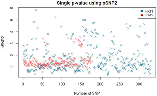
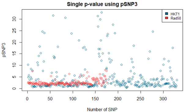
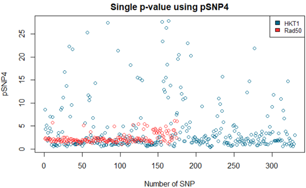
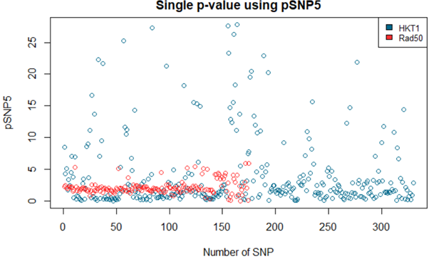
Figure 6: Plots of $-\log p$ values for a range of SNPs over a gene that is known to be significant ($\sim 330$ SNPS from HKT1, shown in blue online), and a negative control gene, ($\sim 170$ SNPs from Rad50, shown in red online). We illustrate 5 different methods for averaging the $p$ values from the list $1\leq j\leq N$ to obtain a single $p$-value for the whole SNP. Top left: $-\log p$-value for SNP using the minimum (3.11); top right: $-\log p$-value calculated using the mean $p$-value over the list (3.12); centre left: (3.13) the average of $-\log p$-values; centre right: using the mean of scaled $|\theta|$, (3.15); lower left: using the mean of scaled $\theta$ (3.16).

We illustrate the output from two case studies: firstly, we consider about 330 SNPs from the HKT1 gene, which is known to be a significant in the uptake of sodium, so we would expect a strong correlation between sodium levels and certain SNPs on the HKT1 gene. The second case is the RAD50 gene, which is involved with detection of damage in DNA, and subsequent repair. There is no reason to expect this to be correlated to ion uptake; so this provides a negative control, only $\sim$170 SNPs on this gene are considered. For both of these genes, only two genetic states are present in the sample, corresponding to $+1$ and $-1$; there are no zero-states.

In Figure 6 we plot the $p$-values for each SNP, with each panel illustrating a different measure (3.11)–(3.16). Results for both genes are shown in the same panel, HKT1 in blue and RAD50 in red. Panel 1 shows that using the minimum value of $p(j)$ (3.11) gives a reasonable separation between SNPs which do not influence phenotype and those that do, although about SNP 150-170 we see several RAD50 SNPs which are moderately significant. For some SNPS, the $-\ln p$ values in this case are quite extreme. Panel 2 has much smaller $p$-values across the whole range, and shows more RAD50 SNPs as significant, hence we conclude that taking the mean $p$-value across all positions in the list as in (3.12) is a poor indicator of significance.

The other three measures (3.13)–(3.16) all show very similar and very good results. Equation (3.13) corresponds to taking the average of the $lnp(j)$-values; in (3.16) we take a weighted average of $\theta_{q}(j)$ values and use that to compute a $p$-value; (3.16) is similar to (3.15), but uses a weighted average of $|\theta|$ values. In all these cases, the $-\ln(p)$-values range from zero to $\sim$30, and the significance of RAD50 SNPs all lie in the range $<10$, with a scatter of HKT1 SNPs being much more significant. These points are clustered around SNPs 25-30, 150-170, 240, 310.

8 Conclusions

We have outlined a Genomic Informational Field Theory (GIFT) which combines knowledge of the genotypes of a population sample with a ranked list of phenotype values to extract information on the strength of interaction between genotype and phenotype. This can be applied to any continuous phenotype measurements, and used across a range of SNPs to determine those which have greatest influence on a particular characteristic. Such analyses will be the topic of future work [3].

We have derived formulae for the calculation of $p$-values in both the biallelic case (3 genetic states labelled $+1,0,-1$) and the mono allelic case (only $+$ and $-$ states). Both derivations a continuum limit of the theory which requires a large value of $N$ – the number of individuals in the sample, and reasonably large number of each genetic state. These $p$-values, together with a choice of significance level (e.g. 5% or 1%) and false discovery rate correction factors, enable one to determine which mutations have a significant impact on phenotype (measured physical characteristic). The model makes no assumptions on the form of the data - it may or may not exhibit Gaussian distribution, it may or may not fit the Hardy-Weinburg assumption ($N_{0}^{2}=4N_{+}N_{-}$). However, in Section 5 we find a few special properties that hold in the case of phenotype distributions which are Gaussian, in particular, if the distributions for the various genotypes have the same variance, and similar means, then the field strength is approximately linear in phenotype value, and the shape $\theta-$path is simply a multiple of the rescaled Gaussian distribution. For more general distributions these properties are no longer hold, but the shape of the $\theta$ trajectory and the form of the field are still meaningful.

The mathematics underlying the model relies on a combination of Shannon’s Information theory [16] and variational calculus [7] to relate information content to a postulated field which describes the relationship between genotype and phenotype. We outline how to determine field-strength from data. Preliminary numericaly studies show this method highlights more genes as having an influence on phenotype than classic GWAS; this is due to the ability to distinguish between negative controls (SNPs which have no influence on phenotype) and SNPS which have a weak influence. In the cases where genotype influences phenotype, we have introduced a field $u_{\pm}(j)$ which quantifies the strength and form of interaction between genetic states $\pm 1,0$ and phenotype. Preliminary results, both theoretical and numerical, show that monotone fields are due to genotype causing a shft in the mean of the phenotype distribution between different genotypes, as illustrated in (5.5) and Figure 5, whilst more general fields can indicate the genotype causing a change in standard deviation of the phenotype distributions (5.6).

In future work, we propose to use these techniques to study the genome of arabidopsis [3], includeing SNPs which are genuinely bi-allelic - that is - where the zero state is present in the sample, along with with the +1 and -1 states, and use larger samples, so that the informational fields can be explored. We also propose to study in more detail the relationship between these methods and the work of Fisher, to explore the various sources of variance in phenotype values, and to analyse cases where a single field can be used to analyse the phenotype-genotype correlation [15].

Acknowledgements

We thank the referees for their helpful suggestions on ways to improve the manuscript. We are grateful to the UKRI-funded Physics of Life network for funding the work of PK.

Conflict of interest

The authors declare that they have no conflict of interest.

Appendix A Calculation of the Variational Derivative

The equation relating the field strength $u_{\pm}$ to the genotype distribution functions $w_{q}(j)$ in Section 4 comes from a variational derivative. We solve this is Euler-Lagrange problem with constraints using Lagrange multipliers. We wish to find stationary points of the action (4.7)

$$\mathcal{A}[\mathbf{w},\boldsymbol{\alpha},\boldsymbol{\beta}]= \;S[\mathbf{w}]-E[\mathbf{w}]+\sum_{j=1}^{N}\alpha_{j}C_{j}(\mathbf{w})+\sum_{r\in\{+1,0,-1\}}\beta_{r}C_{r}(\mathbf{w}),$$ (A1)

where the terms $C_{*}(\mathbf{w})$ represent constraints of the form $C_{*}(\mathbf{w})=0$ that must be satisfied, as detailed in equation (4.2), and $\mathbf{w}=(w_{+}(j),w_{0}(j),w_{-}(j))$, $\boldsymbol{\alpha}=(\alpha_{1},\alpha_{2},\ldots,\alpha_{N})$, $\boldsymbol{\beta}=(\beta_{+},\beta_{0},\beta_{-})$.

To derive the corresponding constrained Euler-Lagrange equations, we allow all the local genotype probabilities $\mathbf{w}$ to be perturbed from $\mathbf{w}=(w_{+}(j),w_{0}(j),w_{-}(j))$ to $\mathbf{w}+h\boldsymbol{\delta}$, where $h\ll 1$ is a small scalar quantity, and $\boldsymbol{\delta}=(\delta_{+}(j),\delta_{0}(j),\delta_{-}(j))$ are general $\mathcal{O}(1)$ perturbations, which satisfy certain contraints that will be derived later (A6).

We consider the first Fréchet derivative of $\mathcal{A}[\mathbf{w},\boldsymbol{\alpha}]$, which is the difference in the Action between the perturbed state and the original state in the limit of small $h$, that is

$$\mathcal{A}^{\prime}[\mathbf{w},\boldsymbol{\alpha},\boldsymbol{\beta}]\delta_{q}(j)= \;\lim_{h\rightarrow 0}h^{-1}\left(\mathcal{A}[\mathbf{w}+h\boldsymbol{\delta},\boldsymbol{\alpha},\boldsymbol{\beta}]-\mathcal{A}[\mathbf{w},\boldsymbol{\alpha},\boldsymbol{\beta}]\right),$$ (A2)

which implies

$$\mathcal{A}^{\prime}[\mathbf{w},\boldsymbol{\alpha},\boldsymbol{\beta}]\delta_{q}= \;\delta_{q}(j)\,\left(1+\log w_{q}(j))+u_{q}(j)+\beta_{q}+\alpha_{j}\genfrac{}{}{0.0pt}{1}{}{}\right).$$ (A3)

We are interested in ‘stationary’ or ‘critical’ points of the functional $\mathcal{A}$, which correspond to $\mathcal{A}^{\prime}[\mathbf{w},\boldsymbol{\alpha}]\delta_{q}(j)=0$ for all possible $\delta_{q}(j)$. Note that here $\delta_{q}(j)$ are not completely arbitrary, there are constraints which $\delta_{q}(j)$ have to satisfy.

If we perturb the terms involving $\alpha_{j}$ to $\alpha_{j}+h\widehat{\alpha}_{j}$ and take the difference between $h\neq 0$ and $h=0$, then we recover the conserved quantities in (4.2) and (4.4). In general, we have

$$\lim_{h\rightarrow 0}h^{-1}\left(\mathcal{A}[\mathbf{w},\boldsymbol{\alpha}+h\widehat{\boldsymbol{\alpha}},\boldsymbol{\beta}]-\mathcal{A}[\mathbf{w},\boldsymbol{\alpha},\boldsymbol{\beta}]\right)=\widehat{\alpha}_{j}C_{j}(\mathbf{w}),$$ (A4)

and so by considering each component of $\boldsymbol{\alpha}$ variable in turn, we obtain each contraint $C_{j}=0$ (4.2). The constraints (4.4) are recovered by considering perturbations of $\boldsymbol{\beta}=(\beta_{+},\beta_{0},\beta_{-})$ to $\boldsymbol{\beta}=(\beta_{+}+\widehat{\beta}_{+},\beta_{0}+\widehat{\beta}_{0},\beta_{-}+\widehat{\beta}_{-})$, that is,

$$\lim_{h\rightarrow 0}h^{-1}\left(\mathcal{A}[\mathbf{w},\boldsymbol{\alpha},\boldsymbol{\beta}+h\widehat{\boldsymbol{\beta}}]-\mathcal{A}[\mathbf{w},\boldsymbol{\alpha},\boldsymbol{\beta}]\right)=\widehat{\beta}_{q}C_{q}(w_{q}(j)).$$ (A5)

Setting this quantity to zero for arbitary $\widehat{\beta}_{q}$ means the constraints $C_{\pm}=0=C_{0}$ are satisfied.

The constraints (4.2) and (4.4) require that $\delta_{q}(j)$ satisfy

$$\delta_{+}(j)+\delta_{0}(j)+\delta_{-}(j)=0\,\;\;\forall j,\qquad\sum_{j=1}^{N}\delta_{+}(j)=0,\quad\sum_{j=1}^{N}\delta_{0}(j)=0,\quad\sum_{j=1}^{N}\delta_{-}(j)=0.$$ (A6)

To satisfy the last set of constraints, we replace $\delta_{0}(j)$ with $-\delta_{+}(j)-\delta_{-}(j)$, this also satisfies the second constraint, provided that the first and third constraints hold. Collecting terms in $\delta_{+}(j)$ and $\delta_{-}(j)$, equation (A3) implies

$$\mathcal{A}^{\prime}[\mathbf{w},\boldsymbol{\alpha},\boldsymbol{\beta}]\delta_{+}(j)= \;\delta_{+}(j)\,\left[\,\beta_{+}-\beta_{0}+u_{+}(j)-u_{0}(j)-\log w_{+}(j)+\log w_{0}(j)\genfrac{}{}{0.0pt}{1}{}{}\,\right],$$

$$\mathcal{A}^{\prime}[\mathbf{w},\boldsymbol{\alpha},\boldsymbol{\beta}]\delta_{-}(j)= \;\delta_{-}(j)\,\left[\,\beta_{-}-\beta_{0}+u_{-}(j)-u_{0}(j)-\log w_{-}(j)+\log w_{0}(j)\genfrac{}{}{0.0pt}{1}{}{}\,\right].$$ (A7)

Since we require $\mathcal{A}`[w_{q},\alpha_{*}]\delta_{q}=0$ for all $\delta_{\pm}(j)$, we obtain the pair of equations

$$u_{+}(j)-u_{0}(j)= \;\log w_{+}(j)-\log w_{0}(j)-\beta_{+}+\beta_{0},$$ (A8)

$$u_{-}(j)-u_{0}(j)= \;\log w_{-}(j)-\log w_{0}(j)-\beta_{-}+\beta_{0},$$ (A9)

which are quoted in the main text (4.8).

Appendix B Master equation approach

The master equation approach refers to a methodology for describing the evolution of a stochastic system using variables to express the probability that a system is in a particular state at time $t$ [9].

We introduce a function which describes the probability of the system being in a certain state. Specifically, we let $G_{\pm}(j,k)$ be the probability that in positions $1,2,\ldots,j$ of the ordered list, there have been $k$ occurrences of the genetic state $\pm$. We can write this formally as $G_{\pm}(j,k)=\mathbb{P}[W_{\pm}(j)=k]$.

By conditioning the probability $\mathbb{P}[W_{+}(j+1)=k+1]$ on the two possible states at $j$ (namely $k$ or $k+1$), that is

$$\mathbb{P}[W_{+}(j+1)=k+1]=\mathbb{P}[W_{+}(j)=k]w_{+}(j+1)+\mathbb{P}[W_{+}(j)=k+1](1-w_{+}(j+1)),$$ (B1)

we obtain a recurrence relation for $G_{\pm}$.

$$G_{+}(j+1,k+1)= \;G_{+}(j,k)w_{+}(j+1)+(1-w_{+}(j+1))G_{+}(j,k+1),$$

$$G_{-}(j+1,k+1)= \;G_{-}(j,k)w_{-}(j+1)+(1-w_{-}(j+1))G_{-}(j,k+1),$$ (B2)

We note that the equations (B2) are almost identical, only differing in the $\pm$ subscripts, so any analysis of the equations can be undertaken on a general case, and the results obtained will be applicable in both the $\pm$ cases, hence, below, we ignore the subscripts. Clearly $k\geq 0$ and $k\leq j$; thus this system has to be solved subject to the boundary conditions $G_{\pm}(j,-1)=0$ and $G_{\pm}(j,j+1)=0$, and the ‘initial’ condition $G(0,0)=1$; here we treat $j$ as a time-variable, with the region $0<j<N$ being the range of interest.

In the case of large $N$, a continuum limit argument can be used to determine the spread of the probability distributions $G(j,k)$, and show that this has the form of a Gaussian distribution. We define a small parameter $h\ll 1$, by $h=1/N$, and a continuum limit of the probability by

$$G(j,k)=h\,\widetilde{G}(\tau,y),\quad\mbox{ where }\;\;\;\tau=h(j-\mbox{$\frac{1}{2}$}),\quad y=h(k+\mbox{$\frac{1}{2}$}),$$ (B3)

The scaling $G=h\widetilde{G}$ is introduced so that the condition $\sum_{k}G(j,k)=1$ for all $j$ is transformed into $\int\widetilde{G}\,{\rm d}y=1$ for all $\tau$.

Following (B2), the governing equation for $\widetilde{G}(\tau,y)$ is

$$\widetilde{G}(\tau+\mbox{$\frac{1}{2}$}h,y+\mbox{$\frac{1}{2}$}h)=\widetilde{w}(\tau+\mbox{$\frac{1}{2}$}h)\widetilde{G}(\tau-\mbox{$\frac{1}{2}$}h,y-\mbox{$\frac{1}{2}$}h)+(1-\widetilde{w}(\tau+\mbox{$\frac{1}{2}$}h))\widetilde{G}(\tau-\mbox{$\frac{1}{2}$}h,y+\mbox{$\frac{1}{2}$}h),$$ (B4)

where $\widetilde{w}(\tau)=w(j+\mbox{$\frac{1}{2}$})$. Shifts of $j,n$ in the definition of continuum limit amount to a choice about which point to perform a Taylor series expanion, and simplify later analysis. The continuum version of the cumulative distribution is defined by $\widetilde{W}(y)=\frac{1}{N}W(j)$, so that $\widetilde{W}(0)=0$ and $\widetilde{W}(1)=w^{(0)}$. Since $w(j)=W(j)-W(j-1)$ we also have $\widetilde{w}(\tau)=\widetilde{W}(\tau)-\widetilde{W}(\tau-h)\approx h\widetilde{W}^{\prime}(\tau)$ and $\widetilde{W}=hW$ together with $\widetilde{W}^{\prime}(\tau)=\widetilde{w}(\tau)$. Taking Taylor series of (B4) in $G$, upto and including terms of $\mathcal{O}(h^{2})$, we find the PDE

$$\frac{\partial\widetilde{G}}{\partial\tau}+\widetilde{w}(\tau)\frac{\partial\widetilde{G}}{\partial y}+\mbox{$\frac{1}{2}$}h(1-\widetilde{w}(\tau))\frac{\partial^{2}\widetilde{G}}{\partial{y}\partial{\tau}}=0.$$ (B5)

We are interested in the solution on the domain $0<\tau<1$ and $0<y<\tau<1$ with $\widetilde{G}(\tau,0)=0=\widetilde{G}(\tau,\tau)=0$, and $G(0,y)=\delta(y)$ (this being the Dirac delta function).

The leading order terms of (B5) are $\widetilde{G}_{\tau}=-\widetilde{w}(\tau)\widetilde{G}_{y}$, which gives the leading order travelling wave solution $\widetilde{G}=\widetilde{G}(y-\widetilde{W}(\tau),\tau)$. At any particular value of $\tau$, the mean of the distribution $G$ is given by $W(j)=N\widetilde{W}(y)$. We define a new variable $z$ for this quantity, and seek a solution of the form

$$\widetilde{G}(\tau,y)=\frac{1}{\sqrt{h}}\check{G}(\tau,z),\quad z=\frac{y-\widetilde{W}(\tau)}{\sqrt{h}}.$$ (B6)

Again the scaling between $\widetilde{G}$ and $\check{G}$ ensures $\int\widetilde{G}\,{\rm d}y=1$ is mapped to $\int\widehat{G}\,{\rm d}z=1$ for all $\tau$. Returning to the second-order expansions of (B5), we obtain an equation of Fokker-Planck type

$$\frac{\partial\widehat{G}}{\partial\tau}=\mbox{$\frac{1}{2}$}\widetilde{w}(\tau)(1-\widetilde{w}(\tau))\frac{\partial^{2}\widehat{G}}{\partial{z}^{2}},$$ (B7)

which has the solution

$$\widehat{G}(\tau,z)=\frac{\mbox{e}^{-z^{2}/4s(\tau)}}{2\sqrt{\pi s(\tau)}},\quad\mbox{ where}\;\;\;\frac{{\rm d}s(\tau)}{{\rm d}\tau}=\mbox{$\frac{1}{2}$}\widetilde{w}(\tau)(1-\widetilde{w}(\tau)).$$ (B8)

Inverting the transformations using (B6) and (B3), we obtain

$$G_{+}(j,k)=\frac{1}{2\sqrt{\pi Ns_{+}(j)}}\exp\left(-\frac{(k-W_{+}(j))^{2}}{4Ns_{+}(j)}\right),\qquad s_{+}(j)=\frac{1}{2N}\sum_{i=1}^{j}w_{+}(i)[1-w_{+}(i)].$$ (B9)

This shows how far from the expected value we would expect to see stochastic fluctuations; similar formula hold for $G_{-},G_{0}$, with corresponding formulae for $s_{-},s_{0}$ in terms of $w_{-}(i),w_{0}(i)$. Since $\theta_{\pm}(j)=W_{\pm}(j)-jw_{\pm}^{(0)}=W_{\pm}(j)-jN_{\pm}/N$, the variance of $\theta_{\pm}(j)$ will be the same as the variance in $W_{\pm}(j)$.

The null hypothesis corresponds to the assumption that the gene has no effect on the phenotype, which is equivaelent to the case of random allocation discussed at the end of Section 4. Here we assume that $\widetilde{w}=w^{(0)}$, hence $W(j)=jw^{(0)}$, $s(j)=w^{(0)}(1-w^{(0)})j/2N$ and so

$$G_{+}(j,k)=\frac{1}{\sqrt{2\pi jw_{+}^{(0)}(1-w_{+}^{(0)})}}\,\exp\left(\frac{-(k-jw_{+}^{(0)})^{2}}{2jw_{+}^{(0)}(1-w_{+}^{(0)})}\right).$$ (B10)

The maximal variance would occur at $j=N/2$ since we require $G(0,k)=\delta_{k,0}$ and $G(N,k)=\delta_{k,N_{q}}$. The combination $k-jw^{(0)}$ corresponds to our $\theta$ variable.

Whilst this approach works well for the early stages in the list, $1\leq j\leq N/2$, for later locations (as $j\nearrow N$), the distibution should reduce in variance, and converge to the single point $G_{q}(N,k)=\delta_{k,N_{q}}$. This PDE approach is not able to describe this type of behaviour. One could work back from this ‘initial’ condition and aim to match the variances of the two continuum solutions: one from $\tau$ increasing from zero and the other with $\tau$ decreasing from 1. The difference between (B10) and the distributions calculated in Section 3 is accounted for by this effect.

Appendix C Phenotypic-dependent distributions

In Section 2, we considered just the location of an individual in an ordered list ($1\leq j\leq N$); in some contexts it may make more sense to think of the distributions $u_{q}(j)$, $W_{q}(j)$, and $\theta_{q}(j)$-paths as functions of phenotype value, $\Omega$, (where $\Omega$ is, for example, height). To model this alternative way of thinking, we define $\widetilde{W}_{q}(\Omega)$ by

$$\widetilde{W}_{q}(\Omega)= \;\mbox{number of individuals of genetic state $q$ with phenotype $<\Omega$},$$ (C1)

$$\widetilde{W}_{q}^{(0)}(\Omega)= q <\Omega$$ expected number of individuals of genetic state with phenotype

(the ‘random’ configuration, i.e. the average over all possible arrangements).

and generalise $\theta_{q}(j)$ to

$$\widetilde{\theta}_{q}(\Omega)=\widetilde{W}_{q}(\Omega)-\widetilde{W}_{q}^{(0)}(\Omega),\qquad q\in\{+1,0,-1\}.$$ (C2)

In general, since the cumulative distribution of $\Omega$, $P(\Omega)$, is unknown, there is no simple expression for $\widetilde{W}_{q}^{(0)}(\Omega)$ similar to (2.7). We define $p(\Omega)=P^{\prime}(\Omega)$ as the probability density function of phenotype.

To relate this phenotypic-dependent formulation with the original (list-based), we write $\Omega(j)$ as the phenotype of individual $j$, and make use of the relations

$$W_{q}(j)=\widetilde{W}_{q}(\Omega(j)),\quad W_{q}^{(0)}(j)=\widetilde{W}_{q}^{(0)}(\Omega(j)),\quad\theta_{q}(j)=\widetilde{\theta}_{q}(\Omega(j)).$$ (C3)

Similarly, the phenotype-dependent fields $\widetilde{u}_{q}(\Omega)$ can be obtained from $\widetilde{u}_{q}(\Omega(j))=u_{q}(j)$; and this field can be related to the local genotype probability density, $\widetilde{w}_{q}(\Omega)$ using an extension to the formula (4.8), namely

$$\widetilde{u}_{+}(\Omega)-\widetilde{u}_{0}(\Omega)= \;\log\widetilde{w}_{+}(\Omega)-\log\widetilde{w}_{0}(\Omega)-\beta_{+}+\beta_{0},$$

$$\widetilde{u}_{-}(\Omega)-\widetilde{u}_{0}(\Omega)= \;\log\widetilde{w}_{-}(\Omega)-\log\widetilde{w}_{0}(\Omega)-\beta_{+}+\beta_{0}.$$ (C4)

In general, the distributions of the phenotypes for the three genotypes could be different, that is, we have distinct probability density functions $p_{+}(\Omega),p_{0}(\Omega),p_{-}(\Omega)$ with corresponding cumulative distributions $P_{+}(\Omega),P_{0}(\Omega),P_{-}(\Omega)$.

If we make the assumption that the three distributions are almost equal, that is

$$P_{q}(\Omega)\approx P(\Omega)+\mathcal{O}(h)\quad\mbox{with}\quad h\ll 1,$$ (C5)

then we can construct the quantity $\widetilde{w}_{q}(\Omega)$ akin to $w_{q}(j)$ (2.5). The expected values of the order statistics $\Omega(j)$ are given by $\mathbb{E}[P(\Omega(j))]=(2j-1)/2N$; taking the difference of this with respect to $j$ gives

$$\mathbb{E}\left[P(\Omega(j))-P(\Omega(j-1)\right]\approx\mathbb{E}\left[P^{\prime}(\Omega)\left(\Omega(j)-\Omega(j-1)\right)\right]=p(\Omega)\Delta\Omega=\frac{1}{N},$$ (C6)

where $\Omega\in(\Omega(j-1),\Omega(j))$. Since the derivative of the cumulative distribution function $P(\Omega)$ is the density function $p(\Omega)$, and $N\gg 1$ we have

$$\Delta\Omega=\Omega(j)-\Omega(j-1)\approx\frac{1}{Np(\Omega)}.$$ (C7)

This describes the expected separation between individual’s phenotypes in the sample $\Gamma$ (2.2).

Combining (2.5), (C3), (C6) noting that, at leading order, the distribution of phenotype states is given by $P(\Omega)$, we obtain

$$w_{q}(j)= \;W_{q}(j)-W_{q}(j\!-\!1)=\widetilde{W}_{q}(\Omega(j))-\widetilde{W}_{q}(\Omega(j\!-\!1))$$

$$\approx \;\frac{{\rm d}\widetilde{W}_{q}}{{\rm d}\Omega}(\Omega(j)-\Omega(j\!-\!1))=\frac{1}{Np(\Omega)}\frac{{\rm d}\widetilde{W}_{q}}{{\rm d}\Omega}=(\Delta\Omega)\frac{{\rm d}\widetilde{W}_{q}}{{\rm d}\Omega}.$$ (C8)

In the case of the expectation of the random configuration, this calculation amounts to a consistency condition

$$w_{q}^{(0)}= \;W_{q}^{(0)}(j)-W_{q}^{(0)}(j-1)=\widetilde{W}_{q}^{(0)}(\Omega(j))-\widetilde{W}_{q}^{(0)}(\Omega(j-1))$$

$$\approx \;\frac{{\rm d}\widetilde{W}_{q}^{(0)}}{{\rm d}\Omega}(\Omega(j)-\Omega(j\!-\!1))\approx\frac{N_{q}}{Np(\Omega)}\frac{{\rm d}P}{{\rm d}\Omega}=\frac{N_{q}}{N}.$$ (C9)

Thus, it is natural to define

$$\widetilde{w}_{q}(\Omega)=\frac{{\rm d}\widetilde{W}_{q}}{{\rm d}\Omega}\Delta\Omega=\frac{{\rm d}\widetilde{W}_{q}}{{\rm d}\Omega}\frac{1}{Np(\Omega)},$$ (C10)

so that we have $\widetilde{w}_{q}=w_{q}^{0}$ in the random case. The interpretation of the paths $(\theta_{+},\theta_{-})$ and $(\widetilde{\theta}_{+},\widetilde{\theta}_{-})$ follow the development of a mathematical model which relates phenotype to genotype via a ‘field’, which is determined using the distributions $W_{q},w_{q},\widetilde{W}_{q},\widetilde{w}_{q}$.

References

• [1] Y Benjamini, Y Hochberg. Controlling the false discovery rate: a practical and powerful approach to multiple testing. J. Roy. Statist. Soc, Ser. B, 57 (1), 289–300. (1995).
• [2] CE Bonferroni, Teoria statistica delle classi e calcolo delle probabilita, Pubblicazioni del R Istituto Superiore di Scienze Economiche e Commerciali di Firenze, (1936).
• [3] S Bray, C Rauch, JAD Wattis, in preparation, (2022).
• [4] S Busoms, P Paajanen, S Marburger, S Bray, X-Y Huang, C Poschenrieder, L Yant, DE Salt. Fluctuating selection on migrant adaptive sodium transporter alleles in coastal Arabidpsis thaliana. Proc Natl Acad Sci, 115, E12443-E12452, (2018).
• [5] RA Fisher. The Correlation between relatives on the supposition of Medelian inheritance. Trans Roy Soc Ed 52, 399-433, (1918).
• [6] G Gibson. Hints of hidden heritability in GWAS. Nature Genetics, 42, 558–560, (2010).
• [7] H Goldstein, Classical Mechanics, Addison-Wesley, (1980).
• [8] C Kittel. Introduction to Solid State Physics, (8th Ed) Wiley, (2018).
• [9] PL Krapivsky, S Redner, E Ben-Naim. A Kinetic view of Statistical Physics. CUP, Cambridge, (2010).
• [10] TA Manolio. Genomewise Association Studies and Assessment of the Risk of Disease. New England J Medicine, 363, 166–177, (2010).
• [11] PAP Moran, CAB Smith. Commentary on RA Fisher’s paper on he correlation between relatives on the supposition of Medelian inheritance. CUP, London, (1966).
• [12] FWJ Olver, A B Olde Daalhuis, DW Lozier, BI Schneider, RF Boisvert, CW Clark, B. R. Miller, B. V. Saunders, H. S. Cohl, and M. A. McClain, eds. NIST Digital Library of Mathematical Functions, CUP, (2010). http://dlmf.nist.gov/, (Eq 5.11.1)
• [13] K Ozaki, Y Ohnishi, A Iida, A Sekine, R Yamada, T Tsunoda, H Sato, H Sato, M Hori, Y Nakamura & T Tanaka. Functional SNPs in the lymphotoxin-$\alpha$ gene that are associated with susceptibility to myocardial infarction. Nature Genetics, 32, 650–654, (2002).
• [14] TA Pearson. How to Interpret a Genome-wide Association Study. J Amer Medical Assoc, 299, 1335–1344, (2008).
• [15] C Rauch, S Blott, P Kyratzi, S Bray, JAD Wattis. GIFT: a new method for the genetic analysis of small gene effects for phenotype values measured with high precision and small population size. in preparation, (2022).
• [16] CE Shannon, A Mathematical Theory of Communication, Bell System Technical Journal, 27, 379–423, & 623–656, (July, & October, 1948).