ABSTRACT

Model selection (MS) and model averaging (MA) are two popular approaches when having many candidate models. Theoretically, the estimation risk of an oracle MA is not larger than that of an oracle MS because the former one is more flexible, but a foundational issue is: does MA offer a substantial improvement over MS? Recently, a seminal work: Peng and Yang, (2021), has answered this question under nested models with linear orthonormal series expansion. In the current paper, we further reply this question under linear nested regression models. Especially, a more general nested framework, heteroscedastic and autocorrelated random errors, and sparse coefficients are allowed in the current paper, which is more common in practice. In addition, we further compare MAs with different weight sets. Simulation studies support the theoretical findings in a variety of settings.

Some key words: Asymptotic efficiency, model averaging, model selection, risk comparison, weight set.

1 Introduction

In the past two decades, model selection (MS) has received growing attention in statistics and econometrics. When a list of candidate models is considered, MS attempts to select a single best model. A large number of MS criteria have been proposed in the literature, including Akaike information criterion (AIC; Akaike,, 1973), Mallows’ $C_{p}$ (Mallows,, 1973), Bayesian information criterion (BIC; Schwarz,, 1978), cross-validation (CV; Allen,, 1974; Stone,, 1974), and so on. Model averaging (MA) is an alternative to MS by taking a weighted average of the estimators/predictions from candidate models, and thus is a smoothed extension of MS, and can potentially reduce risk relative to MS (Yuan and Yang,, 2005; Magnus et al.,, 2010).

Asymptotic efficiency (or asymptotic optimality) is a key theoretical goal pursued in both MS and MA literature. It states that the risk (or loss) of MS (or MA) is equivalent to that of the infeasible oracle candidate model (or averaging estimator/prediction). For MS methods, AIC is asymptotic efficient but BIC is not in the nonparametric framework (Shibata,, 1983; Shao,, 1997); Li, (1987) established the asymptotic efficiency of $C_{p}$ and leave-one-out CV (LOO-CV) for the homoscedastic nonparametric regression; Andrews, (1991) extended the results of Li, (1987) to the case of heteroscedastic errors. See Ding et al., (2018) for a recent review on the properties of MS methods.

For asymptotic optimality of MA, Hansen, (2007) established the asymptotic optimality for Mallows Model Averaging (MMA) when the candidate models are nested and the weights are restricted to a discrete set. Wan et al., (2010) and Zhang, (2021) extended the result of Hansen, (2007) to a non-nested model setting with continuous weights. Hansen and Racine, (2012) established the asymptotic optimality of Jackknife Model Averaging (JMA) for heteroscedastic errors with the weight contained in a discrete set. Zhang et al., (2013) broadened Hansen and Racine, (2012)’s scope of analysis to dependent data and a continuous weight set. Liu and Okui, (2013) proposed a heteroscedasticity-robust model averaging with asymptotic optimality. Ando and Li, (2014, 2017) removed the conventional restriction that the sum of weights equals one in MA and established the asymptotic optimality of JMA for high-dimensional linear models and generalized linear models. Zhao et al., (2016) broadened Ando and Li, (2014)’s scope of analysis to dependent data. Zhang and Wang, (2019), Fang et al., (2019), and Feng et al., (2021) established asymptotic optimality for MA in nonparametric, missing data, and nonlinear models, respectively.

However, most existing literature mainly focuses on optimal properties (e.g., asymptotic efficiency) of MS or MA in their own terms. Although many successful empirical advancements in MA have been demonstrated (see, e.g., Moral-Benito,, 2015; Magnus and Luca,, 2016; Steel,, 2020), theoretical investigations comparing MS and MA are still lacking. Recently, Peng and Yang, (2021) made a seminal contribution to this question. They studied the foundational matter that compares the oracle/optimal MS with MA procedures in a nested model setting with series expansion and have some remarkable findings. However, a limit of Peng and Yang, (2021) is that their study was built with three restrictions: orthonormal design, homoscedastic and independent random errors, and non-sparse coefficients, which could make the study is not applicable in applications. The goal of the current paper is to broaden the scope of analysis of Peng and Yang, (2021) to a general model setting and to answer more important questions. Specifically, our main contributions are as follows.

(i)

Without the three restrictions aforementioned, we answer the questions: does MA offer a significant improvement over MS? If it can happen, when? Moreover, we partition the predictor variables into groups and the group size is allowed to be larger than 1, which leads to a more general nested model framework than that in Peng and Yang, (2021). We define a sequence of indices for grouped variables and find that its decaying order determines when MA is substantially better than MS. As a result, the analysis of Peng and Yang, (2021) becomes a special case of ours. In finite simulation studies, we compare the performance of MMA or JMA with several MS methods, including AIC, BIC, and LOO-CV. The simulation results support our theoretical findings.

(ii)

In MA literature, the MA weights could be chosen from three different weight sets, e.g., the unit simplex (Wan et al.,, 2010; Zhang et al.,, 2013), the unit hypercube (Ando and Li,, 2014, 2017), and the discrete weight set (Hansen,, 2007; Hansen and Racine,, 2012). We further broaden the scope of our work to compare MAs with the weights belonged to these three weight sets.

The rest of the paper is organized as follows. Section 2 provides model setting and four important questions to be answered. Section 3 presents the main results about the comparison of MS and MA. Section 4 considers the comparison of MAs with three different weight sets. Section 5 provides two examples to verify the theoretical results. Section 6 presents the results of finite sample simulations. Section 7 concludes. The proofs of theorems, corollaries, and a lemma are relegated to the Appendix. Supplementary materials contain some additional theoretical results and simulation studies.

2 Model Setting and Questions

Consider the model

$$y_{i}=\mu_{i}+\varepsilon_{i}=\sum_{j=1}^{p_{n}}x_{ij}\beta_{j}+\varepsilon_{i},\quad i=1,\ldots,n,$$ (2.1)

where $\varepsilon_{1},\ldots,\varepsilon_{n}$ are random errors, $x_{i1},\ldots,x_{ip_{n}}$ are nonstochastic predictor variables, and $p_{n}$ $(p_{n}<n)$ is the number of the predictors. In matrix notation, (2.1) can be written as $\bm{y}=\bm{\mu}+\bm{\varepsilon}$, where $\bm{y}=(y_{1},\ldots,y_{n})^{\top}$, $\bm{\mu}=(\mu_{1},\ldots,\mu_{n})^{\top}$, and $\bm{\varepsilon}=(\varepsilon_{1},\ldots,\varepsilon_{n})^{\top}$. We assume that $E(\bm{\varepsilon})=\bm{0}$ and $\text{Cov}(\bm{\varepsilon})=\bm{\Omega}$, where $\bm{\Omega}$ is a positive definite matrix. In the current paper, we use bold forms to denote vectors or matrices.

Following Hansen, (2007, 2014), Feng and Liu, (2020), and Zhang et al., (2020), we consider the nested models, where the $m$th model using the first $\nu_{m}$ predictor variables, such that $0=\nu_{0}<\nu_{1}<\nu_{2}<\cdots<\nu_{q_{n}-1}<\nu_{q_{n}}=p_{n}$, and $q_{n}$ is a positive integer. This nested framework essentially requires that the predictor variables are partitioned into $q_{n}$ groups and the grouped predictors are ordered, where the $m$th group of predictors is $\{x_{i,\nu_{m-1}+1},\ldots,x_{i,\nu_{m}}\}$ and its size is $\nu_{m}-\nu_{m-1}$ for $m=1,\ldots,q_{n}$.

Because some model screening procedures may be implemented prior to MS or MA, without loss of generality, we use the first $M_{n}$ ($2\leq M_{n}\leq q_{n}$) nested candidate models for MS and MA. Let $\mathbf{X}_{m}$ be the $n\times\nu_{m}$ design matrix of the $m$th candidate model. We assume $\mathbf{X}_{m}$ is full of rank for any $m\in\{1,\ldots,M_{n}\}$. Then, under the $m$th model, the estimator of $\bm{\mu}$ is

$$\widehat{\bm{\mu}}_{m}=\mathbf{X}_{m}(\mathbf{X}_{m}^{\top}\mathbf{X}_{m})^{-1}\mathbf{X}_{m}^{\top}\bm{y}\equiv\mathbf{P}_{m}\bm{y},$$

where $\mathbf{P}_{m}=\mathbf{X}_{m}(\mathbf{X}_{m}^{\top}\mathbf{X}_{m})^{-1}\mathbf{X}_{m}^{\top}$ is the hat matrix. A MS method selects an index (say $m^{\star}$) from the index set $\mathcal{H}_{n}=\{1,\ldots,M_{n}\}$ and estimate $\bm{\mu}$ by $\widehat{\bm{\mu}}_{m^{\star}}$ using the selected model. Let $\bm{w}=(w_{1},\ldots,w_{M_{n}})^{\top}$ be a weight vector belonging to the unit simplex of $\mathbb{R}^{M_{n}}$:

$$\mathcal{W}_{n}=\left\{\bm{w}\in[0,1]^{M_{n}}:\sum_{m=1}^{M_{n}}w_{m}=1\right\}.$$

Then, the MA estimator of $\bm{\mu}$ with weight vector $\bm{w}$ is

$$\widehat{\bm{\mu}}(\bm{w})=\sum_{m=1}^{M_{n}}w_{m}\widehat{\bm{\mu}}_{m}=\sum_{m=1}^{M_{n}}w_{m}\mathbf{P}_{m}\bm{y}\equiv\mathbf{P}(\bm{w})\bm{y},$$

where $\mathbf{P}(\bm{w})=\sum_{m=1}^{M_{n}}w_{m}\mathbf{P}_{m}$. The measurement of estimation accuracy is the squared prediction risk, which is defined as $R_{n}(m)=E\{L_{n}(m)\}$ and $R_{n}(\bm{w})=E\{L_{n}(\bm{w})\}$ for MS and MA, respectively, where

$$L_{n}(m)=\|\widehat{\bm{\mu}}_{m}-\bm{\mu}\|^{2}\quad\text{and}\quad L_{n}(\bm{w})=\|\widehat{\bm{\mu}}(\bm{w})-\bm{\mu}\|^{2}$$

are the squared prediction loss for MS and MA, respectively, and $\|\cdot\|^{2}$ is the squared Euclidean norm.

Let $m_{n}^{*}$ be the oracle optimal model index that minimizes $R_{n}(m)$ in $\mathcal{H}_{n}$ and let $\bm{w}_{n}^{*}$ be the oracle optimal weights that minimizes $R_{n}(\bm{w})$ in $\mathcal{W}_{n}$. We assume that $m_{n}^{*}$ and $\bm{w}_{n}^{*}$ are unique. Note that we can not apply $m_{n}^{*}$ and $\bm{w}_{n}^{*}$ in practice, since they are unknown. But using the asymptotically optimal MS and MA procedures mentioned in Section 1, we can select a model index $\widehat{m}_{n}$ and weights $\widehat{\bm{w}}_{n}$, respectively, in the sense that

$${R_{n}(\widehat{m}_{n})\over R_{n}(m_{n}^{*})}\xrightarrow{p}1\quad\text{and}\quad{R_{n}(\widehat{\bm{w}}_{n})\over R_{n}(\bm{w}_{n}^{*})}\xrightarrow{p}1,$$ (2.2)

where $\xrightarrow{p}$ denotes convergence in probability. All limiting processes are studied with respect to $n\to\infty$. Note that in (2.2), $\widehat{m}_{n}$ and $\widehat{\bm{w}}_{n}$ are directly plugged in the expressions $R_{n}(m)$ and $R_{n}(\bm{w})$. Zhang et al., (2020) provided a new type of asymptotical optimality as follows:

$${E\{L_{n}(\widehat{m}_{n})\}\over R_{n}(m_{n}^{*})}\xrightarrow{}1\quad\text{and}\quad{E\{L_{n}(\widehat{\bm{w}}_{n})\}\over R_{n}(\bm{w}_{n}^{*})}\xrightarrow{}1,$$ (2.3)

where the randomness of $\widehat{m}_{n}$ and $\widehat{\bm{w}}_{n}$ are taken into account.

Since MS is a special case of MA with weights concentrating on a single model, it is obvious that $R_{n}(m_{n}^{*})\geq R_{n}(\bm{w}_{n}^{*})$. The first task of this paper is essentially on improvability of the oracle regression model $m_{n}^{*}$ by the oracle MA. Let $\Delta_{n}=R_{n}(m_{n}^{*})-R_{n}(\bm{w}_{n}^{*})$ denote the potential risk reduction of the oracle MA compared to the oracle MS. We first the following two key questions:

• Can $R_{n}(\bm{w}_{n}^{*})$ bring in a smaller order than $R_{n}(m_{n}^{*})$, i.e. can $R_{n}(\bm{w}_{n}^{*})/R_{n}(m_{n}^{*})=o(1)$ happen?

• Is $\Delta_{n}$ a substantial reduction relative to $R_{n}(m_{n}^{*})$ or actually negligible? If both can happen, when is the MA substantially better than MS?

Remark 1.

Write $\bm{x}_{j}=(x_{1j},\ldots,x_{nj})^{\top}$, $j=1,\ldots,p_{n}$. The vectors $\bm{x}_{1},\ldots,\bm{x}_{p_{n}}$ are said to be orthonormal if

$${1\over n}\sum_{i=1}^{n}x_{ij}^{2}=1\quad\text{and}\quad\sum_{i=1}^{n}x_{ij}x_{ik}=0,\quad 1\leq j\neq k\leq p_{n}.$$ (2.4)

Note that (2.4) is satisfied for a nonparametric regression with orthonormal series expansion. Peng and Yang, (2021) has answered Questions Q1 and Q2 under the assumption that the predictors are orthonormal (i.e., (2.4) holds), and the error $\varepsilon_{i}$’s are homoscedastic and independent, which can be restrictive for some applications. In the current paper, we answer the same questions in a more general model setting without the above assumptions. Moreover, Peng and Yang, (2021) used the typical nested framework $\nu_{m}=m$, which is also relaxed in the current paper.

In addition to the weight set $\mathcal{W}_{n}$, there are other two popular weight sets in MA literature: the unit hypercube

$$\mathcal{Q}_{n}=\left\{\bm{w}\in[0,1]^{M_{n}}:0\leq w_{m}\leq 1\right\}$$

and the discrete weight set

$$\mathcal{W}_{n}(N)=\left\{\bm{w}:w_{m}\in\left\{0,{1\over N},{2\over N},\ldots,1\right\},\sum_{m=1}^{M}w_{m}=1\right\}$$

for a fixed positive integer $N$. The weight set $\mathcal{Q}_{n}$ removes the restriction of weights from adding up to 1 in $\mathcal{W}_{n}$. Among MA literature, Ando and Li, (2014) used this weight set to study the optimal MA for the first time in a high-dimensional linear regression setting. Recently, this weight set was further carried to other regression models, e.g., high-dimensional generalized linear model (Ando and Li,, 2017), high-dimensional quantile regression (Wang et al.,, 2021), and high-dimensional survival analysis (Yan et al.,, 2021; He et al.,, 2020). In MA literature, the discrete set $\mathcal{W}_{n}(N)$ is often only considered to establish some asymptotic theories of MA for technical convenience; see, e.g., Hansen, (2007), Hansen and Racine, (2012), and Fang and Liu, (2020). In practice, different weight sets can produce different results, hence the the comparisons of MA with the weight sets are very important. In literature, they are compared by numerical examples; see, for example, Ando and Li, (2014) and Wang et al., (2021). The next task of the current paper is on the theoretical comparison of MA with the weights belonging to different weight sets.

Let $\widetilde{\bm{w}}_{n}^{*}$ and $\bm{w}_{n,N}^{*}$ be the oracle optimal weights that minimizes $R_{n}(\bm{w})$ in $\mathcal{Q}_{n}$ and $\mathcal{W}_{n}(N)$, respectively. We assume that $\widetilde{\bm{w}}_{n}^{*}$ and $\bm{w}_{n,N}^{*}$ are unique. Obviously, $R_{n}(\widetilde{\bm{w}}_{n}^{*})\leq R_{n}(\bm{w}_{n}^{*})\leq R_{n}(\bm{w}_{n,N}^{*})$ since $\mathcal{W}_{n}(N)\subset\mathcal{W}_{n}\subset\mathcal{Q}_{n}$. It implies that the weight relaxation could possibly bring in a smaller optimal risk of MA and the restriction of the weight set $\mathcal{W}_{n}$ to $\mathcal{W}_{n}(N)$ could lead to a larger optimal risk of MA. However, it is unclear that whether the risk reduction of optimal MA by relaxing the weight set $\mathcal{W}_{n}$ to $\mathcal{Q}_{n}$ is substantial and whether the risk increment of optimal MA by restricting the weight set $\mathcal{W}_{n}$ to $\mathcal{W}_{n}(N)$ is substantial. Since $\mathcal{W}_{n}$ is widely used, we use $R_{n}(\bm{w}_{n}^{*})$ as a benchmark for the comparisons. Therefore, we consider the other two key issues as follows:

• Is $R_{n}(\bm{w}_{n}^{*})-R_{n}(\widetilde{\bm{w}}_{n}^{*})$ a substantial reduction relative to $R_{n}(\bm{w}_{n}^{*})$ or actually negligible? If both can happen, when is $\widetilde{\bm{w}}_{n}^{*}$ substantially better than $\bm{w}_{n}^{*}$?

• Is the risk increment $R_{n}(\bm{w}_{n,N}^{*})-R_{n}(\bm{w}_{n}^{*})$ substantial relative to $R_{n}(\bm{w}_{n}^{*})$ or actually negligible? If both can happen, when is $\bm{w}_{n}^{*}$ substantially better than $\bm{w}_{n,N}^{*}$?

The answers to Questions Q1 and Q2 broaden the scope of Peng and Yang, (2021)’s work on advantage of MA over MS. The answers to Questions Q3 and Q4 provide a previously unavailable insight on relative strengths of MA with these three weight sets.

Throughout this paper, we will use the following symbols. For two nonstochastic positive sequences $a_{n}$ and $b_{n}$, $a_{n}\succeq b_{n}$ means $b_{n}=O(a_{n})$, and $a_{n}\asymp b_{n}$ means both $a_{n}\succeq b_{n}$ and $b_{n}\succeq a_{n}$. Also, $a_{n}\sim b_{n}$ means that $a_{n}/b_{n}\to 1$. For two stochastic sequences $a_{n}$ and $b_{n}$, $a_{n}\asymp_{p}b_{n}$ means that $a_{n}=O(b_{n})\{1+o_{p}(1)\}$ and $b_{n}=O(a_{n})\{1+o_{p}(1)\}$; $a_{n}\sim_{p}b_{n}$ means that $a_{n}/b_{n}\to_{p}1$. Let $\lfloor a\rfloor$ be the greatest integer less than or equal to $a$. Let $\lambda_{\min}(\bm{\Omega})$ and $\lambda_{\max}(\bm{\Omega})$ be the minimum and maximum eigenvalues of $\bm{\Omega}$, respectively.

3 Comparisons of MS and MA Procedures

In this section, the goal is to answer Questions Q1 and Q2. We first introduce some important notations and assumptions. Then, we theoretically investigate the comparison of the oracle optimal model $m_{n}^{*}$ and the oracle MA in Subsection 3.2. Last, we extend the obtained results to compare two specific asymptotically optimal MS and MA procedures in Subsection 3.3.

3.1 Grouped Variable Importance

In this subsection, we introduce a notation to measure the importance of each grouped predictors, whose decaying order determines when MA is substantially better than MS that will be shown in Subsection 3.2. Let $\mathbf{X}_{m}^{c}$ be the $n\times(p_{n}-\nu_{m})$ design matrix that consists of the predictors excluded from the $m$th model. Let $\bm{\beta}_{m}=(\beta_{1},\ldots,\beta_{\nu_{m}})^{\top}$ and $\bm{\beta}_{m}^{c}=(\beta_{\nu_{m}+1},\ldots,\beta_{p_{n}})^{\top}$. Then, $\bm{\mu}=\mathbf{X}_{m}\bm{\beta}_{m}+\mathbf{X}_{m}^{c}\bm{\beta}_{m}^{c}$. For convenience, we further assume $\mathbf{X}_{m}$ is full of rank for any $m\in\{M_{n}+1,\ldots,q_{n}\}$. For the $m$th model ($m=1,\ldots,q_{n}$), define

$$\theta_{n,m}={\bm{\beta}_{m-1}^{c\top}\mathbf{X}_{m-1}^{c\top}(\mathbf{I}_{n}-\mathbf{P}_{m-1})\mathbf{X}_{m-1}^{c}\bm{\beta}_{m-1}^{c}-\bm{\beta}_{m}^{c\top}\mathbf{X}_{m}^{c\top}(\mathbf{I}_{n}-\mathbf{P}_{m})\mathbf{X}_{m}^{c}\bm{\beta}_{m}^{c}\over n\mathrm{tr}\{(\mathbf{P}_{m}-\mathbf{P}_{m-1})\bm{\Omega}\}},$$ (3.1)

where $\mathbf{P}_{0}=\bm{0}$. Since the two terms in the numerator of (3.1) measure the importance of the remaining predictors after excluding from the $(m-1)$th model and the $m$th model, respectively, $\theta_{n,m}$ can be regarded as the importance of the $m$th group of variable in some sense. Therefore, we term $\theta_{n,m}$ as the grouped variable importance (GVI).

Next, we impose additional assumptions for the model (2.1) to obtain simple forms of GVI as follows.
Case 1 (Orthonormal design) If the orthonormal design assumption (2.4) is satisfied, it is easy to show that $\bm{\beta}_{m}^{c\top}\mathbf{X}_{m}^{c\top}(\mathbf{I}_{n}-\mathbf{P}_{m})\mathbf{X}_{m}^{c}\bm{\beta}_{m}^{c}=n\|\bm{\beta}_{m}^{c}\|^{2}$. Then, $\theta_{n,m}$ reduces to

$$\theta_{n,m}={\sum_{j=\nu_{m-1}+1}^{\nu_{m}}\beta_{j}^{2}\over\mathrm{tr}\{(\mathbf{P}_{m}-\mathbf{P}_{m-1})\bm{\Omega}\}}.$$

Case 2 (Homoscedastic and uncorrelated errors) If the error terms are homoscedastic and uncorrelated with variance $\sigma^{2}>0$, it is easy to see that $\mathrm{tr}\{(\mathbf{P}_{m}-\mathbf{P}_{m-1})\bm{\Omega}\}=\sigma^{2}(\nu_{m}-\nu_{m-1})$. Then, $\theta_{n,m}$ reduces to

$$\theta_{n,m}={\bm{\beta}_{m-1}^{c\top}\mathbf{X}_{m-1}^{c\top}(\mathbf{I}_{n}-\mathbf{P}_{m-1})\mathbf{X}_{m-1}^{c}\bm{\beta}_{m-1}^{c}-\bm{\beta}_{m}^{c\top}\mathbf{X}_{m}^{c\top}(\mathbf{I}_{n}-\mathbf{P}_{m})\mathbf{X}_{m}^{c}\bm{\beta}_{m}^{c}\over n\sigma^{2}(\nu_{m}-\nu_{m-1})}.$$

Case 3 (Orthonormal design and homoscedastic and uncorrelated errors) If the orthonormal design assumption (2.4) is satisfied and the error terms are homoscedastic and uncorrelated with variance $\sigma^{2}>0$, then $\theta_{n,m}$ has a simple form

$$\theta_{n,m}={\sum_{j=\nu_{m-1}+1}^{\nu_{m}}\beta_{j}^{2}\over\sigma^{2}(\nu_{m}-\nu_{m-1})}.$$

Case 4 (Model setting of Peng and Yang, (2021)) In the model setting of Peng and Yang, (2021), i.e., under the assumptions of the orthonormal design (2.4), the homoscedastic and uncorrelated errors with variance $\sigma^{2}>0$, and the typical nested framework $\nu_{m}=m$, $\theta_{n,m}$ reduces to

$$\theta_{n,m}=\beta_{m}^{2}/\sigma^{2}.$$

From these cases (especially, Cases 1, 3, and 4), the numerator of $\theta_{n,m}$ is determined by the coefficients of the variables in the $m$th group, which further means that $\theta_{n,m}$ is a measure of the grouped variable importance. In the following remark, we provide another explanation for $\theta_{n,m}$.

Remark 2 (Another explanation for $\theta_{n,m}$).

By some simple calculations, we can get a more simple form for $\theta_{n,m}$ as follows

$$\theta_{n,m}={n^{-1}\bm{\mu}^{\top}(\mathbf{P}_{m}-\mathbf{P}_{m-1})\bm{\mu}\over\mathrm{tr}\{(\mathbf{P}_{m}-\mathbf{P}_{m-1})\bm{\Omega}\}}.$$ (3.2)

In the first formula of Appendix A.1, we show that the risk of $\widehat{\bm{\mu}}_{m}$ is

$$R_{n}(m) =E\|\widehat{\bm{\mu}}_{m}-\bm{\mu}\|^{2}$$

$$=\mathrm{tr}\left\{(E\widehat{\bm{\mu}}_{m}-\bm{\mu})(E\widehat{\bm{\mu}}_{m}-\bm{\mu})^{\top}\right\}+\mathrm{tr}\left\{\mathrm{var}(\widehat{\bm{\mu}}_{m})\right\}$$

$$=\bm{\mu}^{\top}(\mathbf{I}_{n}-\mathbf{P}_{m})\bm{\mu}+\mathrm{tr}(\mathbf{P}_{m}\bm{\Omega}),$$

where $\bm{\mu}^{\top}(\mathbf{I}_{n}-\mathbf{P}_{m})\bm{\mu}$ is the trace of the squared bias term of $\widehat{\bm{\mu}}_{m}$ and $\mathrm{tr}(\mathbf{P}_{m}\bm{\Omega})$ is the trace of the variance term of $\widehat{\bm{\mu}}_{m}$, which are non-increasing and increasing in $m$, respectively, because of the nested framework of candidate models. Therefore, by (3.2), the numerator and denominator of $\theta_{n,m}$ are the decrement of the squared bias scared by $n$ and the increment of the variance of risks, respectively, when adding the $m$th group of predictors to the $(m-1)$th model. When $\bm{\Omega}=\sigma^{2}\mathbf{I}_{n}$ and the size of groups is fixed (say $\nu^{\ast}$), the increment of the variance of risks is fixed to be $\nu^{\ast}\sigma^{2}$.

We now impose the following two assumptions for the model (2.1), which are commonly used in the MA literature.

Assumption 1.

$\|\bm{\mu}\|^{2}/n=O(1)$.

Assumption 2.

There are constants $0<c_{1}\leq c_{2}<\infty$ such that $c_{1}<\lambda_{\min}(\bm{\Omega})\leq\lambda_{\max}(\bm{\Omega})<c_{2}$.

Assumption 1 requires the average of $\mu_{i}^{2}$ is bounded. Assumption 2 excludes the degeneracy and divergence of the error terms. Similar assumptions can be found in Wan et al., (2010), Zhang et al., (2013), and Liu et al., (2016). Since $\mathbf{P}_{m}\mathbf{P}_{l}=\mathbf{P}_{\min(m,l)}$ in the nested model setting, it can be easily verified that $\mathbf{P}_{m}-\mathbf{P}_{m-1}$ is a symmetric idempotent matrix, which, together with Assumption 1 yields that $0\leq n^{-1}\bm{\mu}^{\top}(\mathbf{P}_{m}-\mathbf{P}_{m-1})\bm{\mu}\leq\|\bm{\mu}\|^{2}/n<\infty$. Using Assumption 2, we have

$$0<c_{1}(\nu_{m}-\nu_{m-1})<\mathrm{tr}\{(\mathbf{P}_{m}-\mathbf{P}_{m-1})\bm{\Omega}\}<c_{2}(\nu_{m}-\nu_{m-1}).$$

By (3.2) and the truth that $\mathbf{P}_{m}-\mathbf{P}_{m-1}$ is a symmetric idempotent matrix, we know that

$$0\leq\theta_{n,m}<\infty\text{~{}for any $n$ and $m=1,\ldots,q_{n}$}.$$

We further impose an assumption on $\theta_{n,m}$ as follows.

Assumption 3.

For each sufficiently large $n$, $\{\theta_{n,m}:m=1,\ldots,q_{n}\}$ is a non-increasing sequence.

Assumption 3 is an extension of Assumption 1 of Peng and Yang, (2021). The non-increasing ordering of $\{\theta_{n,m}\}_{m=1}^{q_{n}}$ can give us a convenience to characterize the unknown optimal model index $m_{n}^{*}$ and weights $\bm{w}_{n}^{*}$, $\widetilde{\bm{w}}_{n}^{*}$, and $\bm{w}_{n,N}^{*}$, and essentially requires that the predictors are groupwise ordered from the most important to the least important, i.e, the ordering of grouped variables is “correct”. However, different from Peng and Yang, (2021) where the sequence $\{\theta_{n,m}:m=1,\ldots,q_{n}\}$ required to be positive, the current paper allows some components in the sequence to be equal to zeros, i.e., we allow some totally unimportant variables. For the aforementioned Cases 3-4, it means we allow some kind of sparsity of coefficients, which is an important property especially for high-dimensional problems. Under Assumption 3, let $d_{n}=\max\{m\in\{1,\ldots,q_{n}\}:\theta_{n,m}>0\}$ be the number of important groups of predictors. If $d_{n}<q_{n}$, the $m$th group of predictors is not important for $m=d_{n}+1,\ldots,q_{n}$. Next, we make the following assumptions.

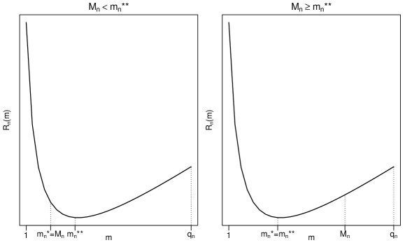
Figure 1: Two typical situations of the squared prediction risk $R_{n}(m)$ and the relationship between $M_{n}$ and $m_{n}^{**}$ under Assumption 6. In left panel: $M_{n}<m_{n}^{**}$. In right penal: $M_{n}\geq m_{n}^{**}$.

Assumption 4.

There exists a constant $V\geq 1$ which does not depend on $m$ and $n$, such that $\max_{1\leq m\leq d_{n}}(\nu_{m}-\nu_{m-1})\leq V$ holds uniformly in large enough $n$.

Assumption 5.

For any fixed $m\in\{1,\ldots,d_{n}\}$, there exist constants $\bar{\theta}_{m}>0$ and $K_{m}>0$ such that $\theta_{n,m}\geq\bar{\theta}_{m}$ for any $n\geq K_{m}$.

Assumption 6.

For each sufficiently large $n$, $R_{n}(m)$ is first decreasing and then increasing when $m$ varies from 1 to $d_{n}$.

Assumption 4 means that when the predictors are partitioned into groups described in Section 2, the sizes of all important groups do not grow to infinity as $n$ increases. Hansen, (2014) and Zhang et al., 2016a also made assumptions on group sizes for the comparison of the risks of estimators by the full model and the MMA. Assumption 5 basically eliminates the case that $\theta_{n,m}$ goes to zero as $n$ increases for any fixed $m\in\{1,\ldots,d_{n}\}$. Thus, it excludes the local-to-zero asymptotic framework with fixed dimensions considered by Hjort and Claeskens, (2003) and Liu, (2015). Note that in the model setting of Peng and Yang, (2021), Assumptions 4–5 are obviously satisfied. Assumption 6 essentially prevents $d_{n}$ from being too small. For example, when $d_{n}\equiv d_{0}$ is fixed as $n\to\infty$ and Assumptions 2 and 5 hold, by (A.1) in the Appendix,

$$R_{n}(m)-R_{n}(m-1) =n\mathrm{tr}\{(\mathbf{P}_{m}-\mathbf{P}_{m-1})\bm{\Omega}\}\biggl{(}{1\over n}-\theta_{n,m}\biggr{)}$$

$$\leq n\mathrm{tr}\{(\mathbf{P}_{m}-\mathbf{P}_{m-1})\bm{\Omega}\}\biggl{(}{1\over n}-\bar{\theta}_{m}\biggr{)}<0$$

for $m=2,\ldots,d_{0}$ and each sufficiently large $n$, which implies that $R_{n}(m)$ is decreasing on $\{1,\ldots,d_{0}\}$ for each sufficiently large $n$ and thus Assumption 6 is not satisfied. Under Assumptions 3 and 5, Assumption 6 is satisfied when $\theta_{n,d_{n}}<{1}/{n}$ for each sufficiently large $n$, which is derived as follows. For a sufficiently large $n$, from Assumptions 3 and 5 and $\theta_{n,d_{n}}<{1}/{n}$, there exists a $m_{n}^{\prime}\in\{2,\ldots,d_{n}-1\}$ such that $\theta_{n,m_{n}^{\prime}}>1/n\geq\theta_{n,m_{n}^{\prime}+1}$. Therefore, when $m=2,\ldots,m_{n}^{\prime}$,

$$R_{n}(m)-R_{n}(m-1)\leq n\mathrm{tr}\{(\mathbf{P}_{m}-\mathbf{P}_{m-1})\bm{\Omega}\}\biggl{(}{1\over n}-\theta_{n,m_{n}^{\prime}}\biggr{)}<0;$$

when $m=m_{n}^{\prime}+1,\ldots,d_{n}$,

$$R_{n}(m)-R_{n}(m-1)\geq n\mathrm{tr}\{(\mathbf{P}_{m}-\mathbf{P}_{m-1})\bm{\Omega}\}\biggl{(}{1\over n}-\theta_{n,m_{n}^{\prime}+1}\biggr{)}\geq 0;$$

and $R_{n}(d_{n})-R_{n}(d_{n}-1)>0$, which together imply that $R_{n}(m)$ is decreasing in $m\in\{1,\ldots,m_{n}^{\prime}\}$ and increasing in $m\in\{m_{n}^{\prime},\ldots,d_{n}\}$. Assumption 6 also implies that $R_{n}(m)$ is first decreasing and then increasing when $m$ increases from $1$ to $q_{n}$ for each sufficiently large $n$. In the derivation of (A.2) in Peng and Yang, (2021), they also used this assumption.

Let $m_{n}^{**}=\arg\min_{m\in\{1,\ldots,q_{n}\}}R_{n}(m)$ be the global optimal model index. We assume that $m_{n}^{**}$ is unique. Note that $m_{n}^{**}$ may not equal to $m_{n}^{*}$ since the number of candidate models $M_{n}$ may be too small to include the $m_{n}^{**}$th model. In fact, under Assumption 6,

$$m_{n}^{*}=\min\{M_{n},m_{n}^{**}\}=\begin{cases}M_{n},&\mathrm{if}~{}M_{n}<m_{n}^{**}\\ m_{n}^{**},&\mathrm{if}~{}M_{n}\geq m_{n}^{**}\end{cases};$$

see Figure 1 which shows two typical situations for $m_{n}^{\ast}$. Peng and Yang, (2021) compared MS and MA under the assumption that $M_{n}$ is large enough to include $m_{n}^{**}$, i.e., $M_{n}\geq m_{n}^{**}$. However, there is a lack of considering on the comparison of MS and MA when $M_{n}<m_{n}^{**}$. In this paper, we also relax this assumption and investigate the impact of $M_{n}$ on the comparison of MS and MA.

In Subsections 3.2–3.3, we shall show that the number of candidate models $M_{n}$ and the decaying order of $\{\theta_{n,m}\}_{m=1}^{d_{n}}$ determine when MA is substantially better than MS.

3.2 A Comparison of Oracle Optimal MS and MA

In this subsection, we answer Questions Q1 and Q2, that is we compare the risks of optimal MS and MA estimators. We begin with the following theorem on the order relationship of $R_{n}(m_{n}^{*})$ and $R_{n}(\bm{w}_{n}^{*})$, which provides an answer to Question Q1.

Theorem 1 (Answer to Question Q1).

Suppose that Assumptions 1-3 and 6 hold. Then, for any sufficiently large $n$,

$$R_{n}(\bm{w}_{n}^{*})\geq{1\over 2}R_{n}(m_{n}^{*}).$$ (3.3)

Moreover, the risks using $m_{n}^{*}$ and $\bm{w}_{n}^{*}$ have the same order, i.e.,

$$R_{n}(m_{n}^{*})\asymp R_{n}(\bm{w}_{n}^{*}).$$ (3.4)

Note that Theorem 1 needs not any restriction on the number of candidate models $M_{n}$, while Peng and Yang, (2021) restricted $M_{n}\geq m_{n}^{**}$. Inequality (3.3) leads to $\Delta_{n}\leq{1\over 2}R_{n}(m_{n}^{*})$ for sufficiently large $n$, which implies that the potential risk reduction of MA compared to MS does not exceed half of optimal risk of MS. Equation (3.4) indicates that while MA has a smaller optimal risk than MS, MA actually cannot reduce the increasing rate (or improve the decreasing rate) of risk by the optimal MS. Thus, even if the oracle model based on MS can be improved by MA, the potential advantage of MA in risk reduction is limited in terms of the increasing/deceasing rate.

We now turn our attention to Question Q2. We first present the following theorem on some elementary properties of the global optimal model index $m_{n}^{**}$, $R_{n}(m_{n}^{*})$, and $R_{n}(\bm{w}_{n}^{*})$, which are important for the subsequent analysis.

Theorem 2.

Suppose that Assumptions 1–6 are satisfied. Then,

• $m_{n}^{**}\to\infty$ as $n\to\infty$;

• $R_{n}(m_{n}^{*})\to\infty$ and $R_{n}(\bm{w}_{n}^{*})\to\infty$ as $n\to\infty$.

Theorem 2(i) indicates that the index of the global optimal model diverges to infinity as $n\to\infty$ under some mild assumptions. For applications, this result tells us that a diverging dimension should be utilized to achieve a promising MS performance. Theorem 2(ii) means that the smallest risks of MS and MA grow to infinity as the sample size $n$ increases. Note that Theorem 2(ii) does not require the restriction $M_{n}\geq m_{n}^{**}$, but this restriction is used in Peng and Yang, (2021).

To investigate the impact of the number of candidate models $M_{n}$ on the comparison of MS and MA, we consider the following two conditions for $M_{n}$.

Condition M1

(Too Small $M_{n}$). $\lim_{n\to\infty}M_{n}/m_{n}^{**}=0$.

Condition M2

(Large Enough $M_{n}$). There exists a constant $\underline{c}>0$ such that $M_{n}/m_{n}^{**}\geq\underline{c}$ when $n$ is large enough.

By Theorem 2(i), under Assumptions 1-6, Condition M1 holds when $M_{n}$ is fixed or diverges to infinity more slowly than $m_{n}^{**}$ as $n\to\infty$. Condition M2 holds when $M_{n}\geq m_{n}^{**}$ considered by Peng and Yang, (2021) or $M_{n}<m_{n}^{**}$ but $M_{n}$ has the same order with $m_{n}^{**}$. Next, we successively explore the degree of improvement $\Delta_{n}/R_{n}(m_{n}^{*})$ by the following theorems under Conditions M1 and M2.

Theorem 3 (Answer to Question Q2 under Condition M1).

Suppose that Assumptions 1-6 hold. Under Condition M1,

$$\Delta_{n}=o\{R_{n}(m_{n}^{*})\}.$$

Theorem 3 implies that when the number of candidate models $M_{n}$ is fixed or diverges to infinity more slowly than $m_{n}^{**}$ as $n\to\infty$, MA has no essential advantage over MS, which again indicates that in applications, an enough large number of candidate models should be utilized. Note that Theorem 3 does not require any assumption of the decaying order of $\{\theta_{n,m}\}_{m=1}^{d_{n}}$.

Furthermore, when Condition M2 holds, we explore the degree of improvement $\Delta_{n}/R_{n}(m_{n}^{*})$ by the following theorem under sensible conditions on $\theta_{n,m}$, which provides an answer to Question Q2 under Condition M2. The answer depends on the decaying order of $\{\theta_{n,m}\}_{m=1}^{d_{n}}$.

Condition A1

(Slowly Decaying $\{\theta_{n,m}\}_{m=1}^{d_{n}}$). There exist constants $k>1$, $0<\delta\leq\eta<1$ with $k\eta<1$, and $K>0$ such that for every integer sequence $\{l_{n}\}$ satisfying $\lim_{n\to\infty}l_{n}=\infty$,

$$\delta\leq\theta_{n,\lfloor kl_{n}\rfloor}/\theta_{n,l_{n}}\leq\eta$$

for any $n\geq K$.

Condition A2

(Fast Decaying $\{\theta_{n,m}\}_{m=1}^{d_{n}}$). For every constant $k>1$ and every integer sequence $\{l_{n}\}$ satisfying $\lim_{n\to\infty}l_{n}=\infty$,

$$\lim_{n\to\infty}\theta_{n,\lfloor kl_{n}\rfloor}/\theta_{n,l_{n}}=0.$$

In the model setting of Peng and Yang, (2021), since $\theta_{n,m}=\beta_{m}^{2}/\sigma^{2}$, Conditions A1–A2 are equivalent to the conditions 1–2 of Peng and Yang, (2021), respectively.

Theorem 4 (Answer to Question Q2 under Condition M2).

Suppose that Assumptions 1-6 and Condition M2 holds. Under Condition A1, we have

$$\Delta_{n}\asymp R_{n}(m_{n}^{*}).$$

Under Condition A2, we have

$$\Delta_{n}=o\{R_{n}(m_{n}^{*})\}.$$

From Theorems 1 and 4, under Condition A1,

$${1\over 2}\leq\liminf_{n\to\infty}{R_{n}(\bm{w}_{n}^{*})\over R_{n}(m_{n}^{*})}\leq\limsup_{n\to\infty}{R_{n}(\bm{w}_{n}^{*})\over R_{n}(m_{n}^{*})}\leq 1-c^{*}$$

for some $c^{*}\in(0,1/2]$; and under Condition A2, $R_{n}(\bm{w}_{n}^{*})\sim R_{n}(m_{n}^{*})$. Therefore, when the number of candidate models $M_{n}$ is large enough, there is a phase transition for the advantage of MA over MS. When $\theta_{n,m}$ decays slowly in $m$, the oracle MA can reduce the optimal risk of MS by a substantial fraction; when $\theta_{n,m}$ decays fast in $m$, MA has no real advantage over MS.

To gain a better understanding of Conditions A1–A2, we make the following more simple conditions (i.e., Assumption 7 and Conditions B1–B2), which imply Conditions A1–A2 by Lemma 1 below.

Assumption 7.

There exists a sequence $\theta_{m}^{*}>0$ for $m=1,\ldots,d_{n}$ such that

$$\sup_{1\leq m\leq d_{n}}\left|{\theta_{n,m}\over\theta_{m}^{*}}-1\right|\to 0\mathrm{~{}as~{}}n\to\infty.$$

Condition B1

(Slowly Decaying $\theta_{m}^{*}$). There exist constants $k>1$ and $0<\delta^{*}\leq\eta^{*}<1$ with $k\eta^{*}<1$ such that $\delta^{*}\leq\theta_{\lfloor km\rfloor}^{*}/\theta_{m}^{*}\leq\eta^{*}$ when $m$ is large enough.

Condition B2

(Fast Decaying $\theta_{m}^{*}$). For every constant $k>1$, $\lim_{m\to\infty}\theta_{\lfloor km\rfloor}^{*}/\theta_{m}^{*}=0$.

Lemma 1.

Suppose that Assumption 7 holds. Then, Conditions B1–B2 imply Conditions A1–A2, respectively.

Assumption 7 implies that $\lim_{n\to\infty}\theta_{n,m}=\theta_{m}^{*}$ for any fixed $m$. Thus, Assumption 7 can lead to Assumption 5 by taking $\bar{\theta}_{m}=\theta_{m}^{*}/2$. Condition B1 is satisfied for $\theta_{m}^{*}\sim m^{-2\alpha}$ or slightly more generally for $\theta_{m}^{*}\sim m^{-2\alpha}(\log m)^{\beta}$ with constants $\alpha>1/2$ and $\beta\in\mathbb{R}$. Condition B2 is satisfied for the exponential-decay case, that is, $\theta_{m}^{*}\sim\exp(-cm)$ for some $c>0$. These two types of decaying rates are commonly used in the literature. For example, in the research of infinite-order autoregressive (AR) models, Ing and Wei, (2005), Ing, (2007), and Liao et al., (2021) considered the exponential-decay and algebraic-decay cases for the AR coefficients, which are described in our context as follows:

• Exponential-decay case: $C_{1}m^{-\tau_{1}}e^{-cm}\leq\theta_{m}^{*}\leq C_{2}m^{\tau_{1}}e^{-cm}$, where $C_{1}$, $C_{2}$, $\tau_{1}$, and $c$ are some constant with $C_{2}\geq C_{1}>0$, $\tau_{1}\geq 0$, and $c>0$.

• Algebraic-decay case: $(C_{3}-C_{4}m^{-\tau_{2}})m^{-\bar{\alpha}}\leq\theta_{m}^{*}\leq(C_{3}+C_{4}m^{-\tau_{2}})m^{-\bar{\alpha}}$, where $C_{3}$, $C_{4}$, $\tau_{2}$, and $\bar{\alpha}>1$ are some positive constants.

It can be easily verified that the exponential-decay case (i) and the algebraic-decay case (ii) satisfy Condition B2 and Condition B1, respectively.

3.3 A Comparison of Two Specific MS and MA Procedures

Up to now, the theoretical results of Theorems 1 and 3–4 mainly focus on the comparison of oracle optimal MS and MA, not directly on the comparison of two specific MS and MA procedures. Fortunately, by using (2.2) and (2.3), we can do the latter comparison by connecting the feasible risks (when using a selected model index or weights from some methods) and infeasible risks (when using the oracle model index or weights). In literature, the proof of asymptotic efficiency (or optimality) of MS and MA requires the smallest risks of MS and MA (i.e., $R_{n}(m_{n}^{*})$ and $R_{n}(\bm{w}_{n}^{*})$ in our notations) to grow to infinity as the sample size increases, respectively. Both have been verified in Theorem 2(ii) under Assumptions 1–6.

Let $\widehat{m}_{n}$ and $\widehat{\bm{w}}_{n}$ be the selected model index and chosen weights based on asymptotically optimal MS and MA methods, respectively. Then, we have the following two consequences.

Corollary 1.

Suppose that Assumptions 1-6 hold, and $\widehat{m}_{n}$ and $\widehat{\bm{w}}_{n}$ are asymptotically optimal in the sense of (2.2), i.e., $R_{n}(\widehat{m}_{n})/R_{n}(m_{n}^{*})\to_{p}1$ and $R_{n}(\widehat{\bm{w}}_{n})/R_{n}(\bm{w}_{n}^{*})\to_{p}1$. Then,

• the risks using $\widehat{m}_{n}$ and $\widehat{\bm{w}}_{n}$ have the same order, i.e., $R_{n}(\widehat{m}_{n})\asymp_{p}R_{n}(\widehat{\bm{w}}_{n})$;

• under Conditions M2 and A1, the MA using $\widehat{\bm{w}}_{n}$ essentially improves over the MS using $\widehat{m}_{n}$, i.e., $R_{n}(\widehat{m}_{n})-R_{n}(\widehat{\bm{w}}_{n})\asymp_{p}R_{n}(\widehat{m}_{n})$;

• under Condition M1 or Conditions M2 and A2, $\widehat{m}_{n}$ and $\widehat{\bm{w}}_{n}$ are asymptotically equivalent in risk, i.e., $R_{n}(\widehat{m}_{n})\sim_{p}R_{n}(\widehat{\bm{w}}_{n})$.

Corollary 2.

Suppose that Assumptions 1-6 hold, and $\widehat{m}_{n}$ and $\widehat{\bm{w}}_{n}$ are asymptotically optimal in the sense of (2.3), i.e., $E\{L_{n}(\widehat{m}_{n})\}/R_{n}(m_{n}^{*})\to 1$ and $E\{L_{n}(\widehat{\bm{w}}_{n})\}/R_{n}(\bm{w}_{n}^{*})\to 1$. Then, the results of Corollary 1 hold when $R_{n}(\widehat{m}_{n})$, $R_{n}(\widehat{\bm{w}}_{n})$, $\asymp_{p}$, and $\sim_{p}$ are replaced by $E\{L_{n}(\widehat{m}_{n})\}$, $E\{L_{n}(\widehat{\bm{w}}_{n})\}$, $\asymp$, and $\sim$, respectively.

Since the proofs of Corollaries 1 and 2 are similar, we only give the proof of Corollary 1 in Appendix A.6.

4 Comparisons of MAs with Different Weight Sets

In this section, we shall compare the optimal risks of MAs when the weights belong to three weight sets: $\mathcal{W}_{n}$, $\mathcal{Q}_{n}$, and $\mathcal{W}_{n}(N)$, which provide answers to Questions Q3–Q4.

4.1 A Comparison of MAs with Weight Sets $\mathcal{W}_{n}$ and $\mathcal{Q}_{n}$

In this subsection, we focus on the comparison of the risks of MA estimators when the weights comes from $\mathcal{W}_{n}$ and $\mathcal{Q}_{n}$, respectively. We first present the following theorem, which provides an answer to Question Q3.

Theorem 5 (Answer to Question Q3).

Suppose that Assumptions 1-6 hold. Then,

$$R_{n}(\bm{w}_{n}^{*})-R_{n}(\widetilde{\bm{w}}_{n}^{*})=o\{R_{n}(\bm{w}_{n}^{*})\},$$ (4.1)

i.e., $\bm{w}_{n}^{*}$ and $\widetilde{\bm{w}}_{n}^{*}$ are asymptotically equivalent in risk.

Equation (4.1) indicates that while the weight relaxation could lead to a smaller optimal risk of MA, asymptotically it does not provide any substantial benefit. Note that Theorem 5 does not require any assumptions of the number of candidate models $M_{n}$ and the decaying order of $\{\theta_{n,m}\}_{m=1}^{d_{n}}$.

Furthermore, we compare two specific asymptotically optimal MS and MA procedures, where MA weights are chosen from the weight set $\mathcal{Q}_{n}$. Let $\widehat{\bm{w}}_{n}^{Q}$ be chosen weights based on a specific MA method satisfying the asymptotic optimality (2.2) or (2.3) when the total weight is not constrained (i.e., the total weight constraint $\sum_{m=1}^{M_{n}}w_{m}=1$ is not used). For example, the asymptotic optimality (2.2) of JMA without the total weight constraint has been established by Ando and Li, (2014) and Zhao et al., (2016) for independent data and dependent data, respectively. Using Theorem 5, it is easy to conclude the following corollary on a comparison of MA without the total weight constraint and MS.

Corollary 3.

Suppose that Assumptions 1-6 hold.

• Assume that $\widehat{m}_{n}$ and $\widehat{\bm{w}}_{n}^{Q}$ satisfy $R_{n}(\widehat{m}_{n})/R_{n}(m_{n}^{*})\to_{p}1$ and $R_{n}(\widehat{\bm{w}}_{n}^{Q})/R_{n}(\bm{w}_{n}^{*})\to_{p}1$, then the results of Corollary 1 hold when $\widehat{\bm{w}}_{n}$ is replaced by $\widehat{\bm{w}}_{n}^{Q}$.

• Assume that $\widehat{m}_{n}$ and $\widehat{\bm{w}}_{n}^{Q}$ satisfy $E\{L_{n}(\widehat{m}_{n})\}/R_{n}(m_{n}^{*})\to 1$ and $E\{L_{n}(\widehat{\bm{w}}_{n}^{Q})\}/R_{n}(\bm{w}_{n}^{*})\to 1$, then the results of Corollary 2 hold when $\widehat{\bm{w}}_{n}$ is replaced by $\widehat{\bm{w}}_{n}^{Q}$.

4.2 A Comparison of MAs with Weight Sets $\mathcal{W}_{n}$ and $\mathcal{W}_{n}(N)$

In this subsection, we focus on the comparison of the optimal risks of MA estimators with the weights belonging to the weight sets $\mathcal{W}_{n}$ and $\mathcal{W}_{n}(N)$, respectively. We present the following theorem on an upper bound of $R_{n}(\bm{w}_{n,N}^{*})-R_{n}(\bm{w}_{n}^{*})$ and an answer to Question Q4.

Theorem 6 (Answer to Question Q4).

Suppose that Assumptions 1-6 hold. Then, for any sufficiently large $n$,

$$R_{n}(\bm{w}_{n,N}^{*})-R_{n}(\bm{w}_{n}^{*})\leq{1\over 2N}R_{n}(m_{n}^{*}).$$ (4.2)

Furthermore, under Conditions M2 and A1, we have

$$R_{n}(\bm{w}_{n,N}^{*})-R_{n}(\bm{w}_{n}^{*})\asymp R_{n}(\bm{w}_{n}^{*});$$

and under Condition M1 or Conditions M2 and A2, we have

$$R_{n}(\bm{w}_{n,N}^{*})-R_{n}(\bm{w}_{n}^{*})=o\{R_{n}(\bm{w}_{n}^{*})\},$$

i.e.,

$$R_{n}(\bm{w}_{n,N}^{*})\sim R_{n}(\bm{w}_{n}^{*}).$$

Observe that $R_{n}(\bm{w}_{n,1}^{*})=R_{n}(m_{n}^{*})$. Therefore, Theorems 1 and 3–4 are special cases of Theorem 6 with $N=1$. The upper bound in (4.2) implies that for a fixed and sufficiently large sample size, $R_{n}(\bm{w}_{n,N}^{*})$ can be made arbitrarily close to $R_{n}(\bm{w}_{n}^{*})$ as $N$ is large enough, which is expected since $\mathcal{W}_{n}(N)$ approaches $\mathcal{W}_{n}$ as close as possible by making $N$ sufficiently large. From Theorem 6, when $M_{n}$ is large enough and $\theta_{n,m}$ decays slowly in $m$, restricting the weight set $\mathcal{W}_{n}$ to $\mathcal{W}_{n}(N)$ can enlarge the optimal risk of MA by a substantial multiple; when $M_{n}$ is too small or $M_{n}$ is large enough and $\theta_{n,m}$ decays fast in $m$, MA restricted to the discrete weight set has no real disadvantage over MA with $\mathcal{W}_{n}$. In the Supplementary Material, we further present a comparison of MAs with nested discrete weight sets.

5 Two Examples

In this section, we provide two examples to verify the theoretical results of Theorems 3–4 and 6, whose detailed derivations are given in Appendix A.10. Given $a,b>0$, the incomplete beta function is defined by $B(x;a,b)=\int_{0}^{x}t^{a-1}(1-t)^{b-1}\,dt$ for $0\leq x\leq 1$.

In these two examples, we consider the model setting of Peng and Yang, (2021), that is model (2.1) with orthonormal design assumption (2.4), homoscedastic and uncorrelated error terms and $\nu_{m}=m$ for $m=1,\ldots,p_{n}$.

Example 5.1 (Slowly Decaying $\theta_{n,m}$). The true coefficients are set to $\beta_{m}=m^{-\alpha}$ with $\alpha>1/2$. Then, $\theta_{n,m}=m^{-2\alpha}/\sigma^{2}$ and Condition A1 is satisfied. By some simple calculations, we can get $m_{n}^{**}\sim({n\over\sigma^{2}})^{{1\over 2\alpha}}$. We consider the following two situations on the number of candidate models $M_{n}$.

(i) When $\lim_{n\to\infty}M_{n}/m_{n}^{**}=0$, we have

$${1\over n}R_{n}(\bm{w}_{n,N}^{*})\sim{1\over n}R_{n}(\bm{w}_{n}^{*})\sim\begin{cases}\sum_{m=M+1}^{\infty}m^{-2\alpha},&\text{if}~{}M_{n}\equiv M~{}\text{is fixed as}~{}n\to\infty,\\ {M_{n}^{-2\alpha+1}\over 2\alpha-1},&\text{if}~{}\lim_{n\to\infty}M_{n}=\infty~{}\text{but}~{}M_{n}=o(m_{n}^{**}).\end{cases}$$

This verifies that $R_{n}(\bm{w}_{n,N}^{*})\sim R_{n}(\bm{w}_{n}^{*})$ under Condition M1, which accords with Theorem 3 and the third conclusion of Theorem 6.

(ii) When $M_{n}/m_{n}^{**}\geq\underline{c}$ for some $\underline{c}>0$, we have

$${1\over n}R_{n}(\bm{w}_{n,N}^{*})\asymp{1\over n}R_{n}(\bm{w}_{n}^{*})\asymp n^{-{2\alpha-1\over 2\alpha}}.$$

By a simple calculation, we know that $R_{n}(\bm{w}_{n,N}^{*})-R_{n}(\bm{w}_{n}^{*})$ is lower bounded by ${\varpi\sigma^{2}\over 2^{2\alpha+1}\varpi^{-2\alpha}+2}\left({n\over\sigma^{2}}\right)^{{1\over 2\alpha}}$, where $\varpi=\min\{\underline{c},(2N-1)^{-{1\over 2\alpha}}\}$. Moreover, if $\lim_{n\to\infty}M_{n}/m_{n}^{**}=\kappa$, $\kappa\in(0,\infty]$ and $M_{n}=o(p_{n})$, we have

$$\lim_{n\to\infty}{R_{n}(\bm{w}_{n}^{*})\over R_{n}(\bm{w}_{n,N}^{*})}={1\over\psi_{N}^{*}+{\kappa^{-2\alpha+1}\over 2\alpha}}\left[{2\alpha-1\over 4\alpha^{2}}\left\{{\pi\over\sin({\pi\over 2\alpha})}-B\left({1\over 1+\kappa^{2\alpha}};1-{1\over 2\alpha},{1\over 2\alpha}\right)\right\}+{\kappa^{-2\alpha+1}\over 2\alpha}\right],$$

where $\psi_{N}^{*}$ is defined in Appendix A.10. Furthermore, we can show that

$$\lim_{n\to\infty}{R_{n}(\bm{w}_{n}^{*})\over R_{n}(\bm{w}_{n,N}^{*})}<1,$$

which verifies that $R_{n}(\bm{w}_{n,N}^{*})-R_{n}(\bm{w}_{n}^{*})\asymp R_{n}(\bm{w}_{n}^{*})$, which accords with the first conclusion of Theorem 4 and the second conclusion of Theorem 6. Figure 2(a) plots $\lim_{n\to\infty}{R_{n}(\bm{w}_{n}^{*})\over R_{n}(\bm{w}_{n,N}^{*})}$ againsts $N\in\{1,\ldots,10\}$ for $\kappa=0.5,1,2$ and Figure 2(b) plots $\lim_{n\to\infty}{R_{n}(\bm{w}_{n}^{*})\over R_{n}(\bm{w}_{n,N}^{*})}$ againsts $\kappa\in(0,8)$ for $N=1,2,4$, where $\alpha=0.8$, which further verifies that $\lim_{n\to\infty}{R_{n}(\bm{w}_{n}^{*})\over R_{n}(\bm{w}_{n,N}^{*})}<1$.

Example 5.2 (Fast Decaying $\theta_{n,m}$). The true coefficients are set to $\beta_{m}=\exp(-cm)$ with $c>0$. Then, $\theta_{n,m}=\exp(-2cm)/\sigma^{2}$ and Condition A2 is satisfied. The global optimal model should include the first $m_{n}^{**}\sim{1\over 2c}\log\left({n\over\sigma^{2}}\right)$ terms. We consider the following three situations on the number of candidate models $M_{n}$.

(i) When $\limsup_{n\to\infty}M_{n}/m_{n}^{**}<1$, we have

$${1\over n}R_{n}(\bm{w}_{n,N}^{*})\sim{1\over n}R_{n}(\bm{w}_{n}^{*})\sim{\exp(-2cM_{n})\over\exp(2c)-1},$$

which verifies that $R_{n}(\bm{w}_{n,N}^{*})\sim R_{n}(\bm{w}_{n}^{*})$ under Condition M1 and accords with Theorem 3 and the third conclusion of Theorem 6.

(ii) When $M_{n}<m_{n}^{**}$ for any sufficiently large $n$ but $\lim_{n\to\infty}M_{n}/m_{n}^{**}=1$, we have

$${1\over n}R_{n}(\bm{w}_{n,N}^{*})\sim{1\over n}R_{n}(\bm{w}_{n}^{*})\sim{1\over 2c}{\sigma^{2}\over n}\log\left({n\over\sigma^{2}}\right)+{\exp(-2cM_{n})-\exp(-2cp_{n})\over\exp(2c)-1},$$

which verifies that $R_{n}(\bm{w}_{n,N}^{*})\sim R_{n}(\bm{w}_{n}^{*})$ under Conditions M2 and A2, and accords with the second conclusion of Theorem 4 and the third conclusion of Theorem 6.

(iii) When $M_{n}\geq m_{n}^{**}$ for any sufficiently large $n$, we have

$${1\over n}R_{n}(\bm{w}_{n,N}^{*})\sim{1\over n}R_{n}(\bm{w}_{n}^{*})\sim{1\over 2c}{\sigma^{2}\over n}\log\left({n\over\sigma^{2}}\right).$$

which also verifies that $R_{n}(\bm{w}_{n,N}^{*})\sim R_{n}(\bm{w}_{n}^{*})$ under Conditions M2 and A2, and accords with the second conclusion of Theorem 4 and the third conclusion of Theorem 6.

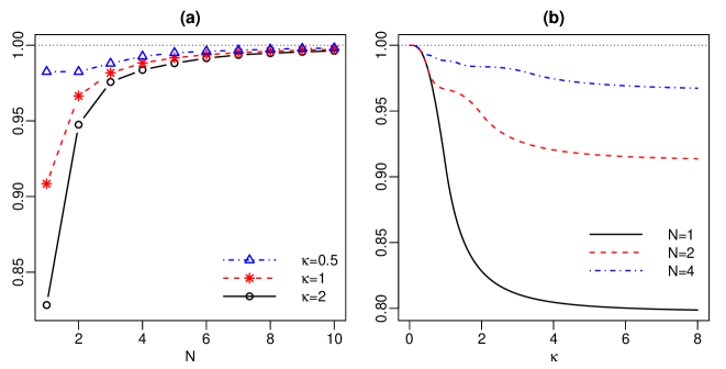
Figure 2: Numerical illustration for Example 5.1 with $\alpha=0.8$. Left: plots of $\lim_{n\to\infty}{R_{n}(\bm{w}_{n}^{*})\over R_{n}(\bm{w}_{n,N}^{*})}$ against $N\in\{1,\ldots,10\}$ for $\kappa=0.5,1,2$, respectively. Right: plots of $\lim_{n\to\infty}{R_{n}(\bm{w}_{n,dN}^{*})\over R_{n}(\bm{w}_{n,d}^{*})}$ againsts $\kappa\in(0,8)$ for $N=1,2,4$, respectively.

6 Simulation Studies

In this section, we conduct several simulation studies to verify the theoretical results presented in Corollaries 1 and 3, where the specific MS and MA methods are compared. Here we choose AIC, BIC, and LOO-CV as MS methods, and MMA and JMA for MA methods. Specifically, we use the following three examples:

• Example 1: General nested framework (i.e., $\nu_{m}\neq m$), homoscedastic and uncorrelated errors, and (approximately) orthonormal design;

• Example 2: Typical nested framework (i.e., $\nu_{m}=m$), heteroscedastic and autocorrelated errors, and (approximately) orthonormal design;

• Example 3: Typical nested framework (i.e., $\nu_{m}=m$), homoscedastic and uncorrelated errors, and non-orthonormal design.

To evaluate the estimators, we compute the risks of the competing methods by computing averages across 1000 replications. Supplementary materials contain more simulation studies.

Example 1 (General nested framework) We use the same set-up as that of Peng and Yang, (2021) except the coefficients $\beta_{m}$’s. Specifically, suppose the data come from the model (2.1), where $p_{n}=\lfloor 5n^{2/3}\rfloor$, $x_{i1}=1$, the remaining $x_{ij}$ are independent and identically distributed (iid) from $N(0,1)$, and the random errors $\varepsilon_{i}$ are iid from $N(0,\sigma^{2})$ and are independent of $x_{ij}$’s. The population $R^{2}$ is denoted by $R^{2}=\mathrm{var}(\mu_{i})/\mathrm{var}(y_{i})$, which is controlled in $0.25$, $0.5$ or $0.75$ via the parameter $\sigma^{2}$. We consider a more general nested model setting than that of Peng and Yang, (2021) by setting

$$\nu_{m}=\begin{cases}5\lfloor m/2\rfloor+2,&m~{}\text{is odd}\\ 5\lfloor m/2\rfloor,&m~{}\text{is even}\end{cases},\quad m=1,\ldots,q_{n}-1$$

and $\nu_{q_{n}}=p_{n}$. Thus, the size of the $m$th group of predictors is 2 when $m$ is odd and 3 when $m$ is even, $m=1,\ldots,q_{n}-1$. We consider two cases with different coefficient decaying orders:

• Case 1. $\beta_{j}=m^{-\alpha_{1}}$ when $x_{ij}$ is in the $m$th group and $\alpha_{1}$ is set to be 1, 1.5 or 2.

• Case 2. $\beta_{j}=\exp(-\alpha_{2}m)$ when $x_{ij}$ is in the $m$th group and $\alpha_{2}$ is set to be 1, 1.5 or 2.

For Case 1, we know that $\theta_{n,m}$ converges to $\theta_{m}^{*}=m^{-2\alpha_{1}}/\sigma^{2}$ in probability and then Condition B1 is satisfied (in our theories, we take the predictors as fixed, but in simulation, they are random. When verifying our conditions, we do not consider this randomness), and for Case 2, $\theta_{n,m}$ converges to $\theta_{m}^{*}=\exp(-2\alpha_{2}m)/\sigma^{2}$ in probability and then Condition B2 is satisfied. The sample size $n$ varies at 50, 500, 1000, 2000, 3000, and 4000. The number of candidate models is determined by $M_{n}=\mathrm{INT}(3n^{1/3})$, where the function $\mathrm{INT}(a)$ returns the nearest integer from $a$. In each simulation setting of the combination of $n$, $R^{2}$, and $\alpha_{1}$ (or $\alpha_{2}$), we normalize the risks of the MS methods by dividing by the risk of MMA.

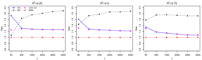
(a)

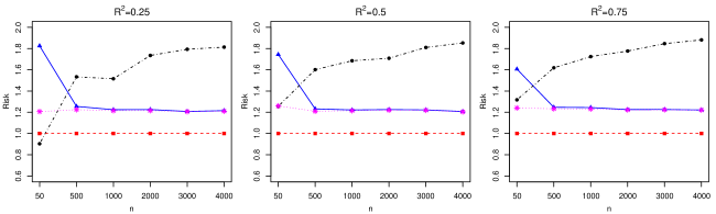
(b)

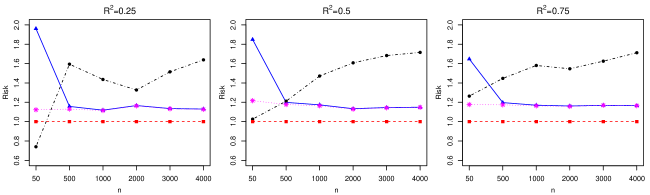
(c)

Figure 3: Simulation results for Example 1 with the case of slowly decaying $\theta_{m}^{*}$. Normalized risk functions for AIC, BIC, LOO-CV, and MMA when $\theta_{m}^{*}=m^{-2\alpha_{1}}/\sigma^{2}$ with $\alpha_{1}=1$ in row (a), $\alpha_{1}=1.5$ in row (b), and $\alpha_{1}=2$ in row (c).

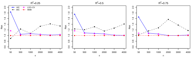
(a)

(b)

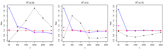
(c)

Figure 4: Simulation results for Example 1 with the case of fast decaying $\theta_{m}^{*}$. Normalized risk functions for AIC, BIC, LOO-CV, and MMA when $\theta_{m}^{*}=\exp(-2\alpha_{2}m)/\sigma^{2}$ with $\alpha_{2}=1$ in row (a), $\alpha_{2}=1.5$ in row (b), and $\alpha_{2}=2$ in row (c).

Simulation results are summarized in Figures 3–4. In each figure, the simulation results with three different coefficient decaying orders are displayed in rows (a), (b), and (c), respectively. Note that Figure 3 are under Case 1 (slowly decaying coefficients) and Figure 4 are under Case 2 (fast decaying coefficients). Since both AIC and LOO-CV are asymptotically optimal for Example 1, as expected, their performances are very close for large sample size. In the slowly decaying $\theta_{m}^{*}$ case, the performance gap between AIC (or LOO-CV) and MMA does not vanish when $n$ increases, while in the fast decaying $\theta_{m}^{*}$ case, it becomes very small when $n$ is large, which are consistent with the results of Corollary 1.

Following Peng and Yang, (2021), we also include BIC in our simulation, although often, BIC is not asymptotically optimal. In Case 1, the advantage of AIC over BIC becomes increasingly larger as $n$ increases from 50 to 4000, while in Case 2 with fast decaying $\theta_{m}^{*}$, BIC is competitive with AIC in some scenarios. This phenomenon was also observed by Peng and Yang, (2021).

Example 2 (Heteroscedastic and autocorrelated errors) The setting of this example is the same as that of Example 1 except that the typical nested framework with $\nu_{m}=m$ and heteroscedastic and autocorrelated errors are considered. We utilize the same error process of Zhang et al., (2013) that is both heteroscedastic and autocorrelated. Specifically, the error process is given by $\varepsilon_{i}=\varepsilon_{i1}+\varepsilon_{i2}$, $\varepsilon_{i1}$’s are independent observations from the $N(0,x_{i2}^{2})$ distribution, and $\varepsilon_{i2}$ follows an AR(1) process with an autocorrelation coefficient $\rho_{1}=0.5$, where $\varepsilon_{i2}=\rho_{1}\varepsilon_{i-1,2}+e_{i}$, $\varepsilon_{12}\sim N(0,1)$, and $e_{i}$’s are iid from $N(0,1-\rho_{1}^{2})$ and are independent of $\varepsilon_{i2}$’s. Then, the covariance matrix of $\bm{\varepsilon}$ given $x_{ij}$’s is $\bm{\Omega}=\bm{\Omega}_{1}+\bm{\Omega}_{2}$, where $\bm{\Omega}_{1}=\mathrm{diag}\{x_{12}^{2},\ldots,x_{n2}^{2}\}$ and $\bm{\Omega}_{2}=(\rho_{1}^{|k-l|})_{k,l=1,\ldots,n}$. By a simple calculation, we have

$$\mathrm{tr}(\mathbf{P}_{m}\bm{\Omega}_{1})\xrightarrow{p}\begin{cases}1,&\nu_{m}=1\\ \nu_{m}+2,&\nu_{m}\geq 2\end{cases},\quad\mathrm{tr}(\mathbf{P}_{m}\bm{\Omega}_{2})\xrightarrow{p}{2\rho_{1}\over 1-\rho_{1}}+\nu_{m}.$$

Therefore, for any fixed $m$, $\theta_{n,m}\to\theta_{m}^{*}=\beta_{m}^{2}/\zeta_{m}$ in probability, where

$$\zeta_{m}=\begin{cases}{2\over 1-\rho_{1}},&m=1,\\ 4,&m=2,\\ 2,&m\geq 3.\end{cases}$$

We consider two cases with different decaying orders of $\theta_{m}^{*}$:

• Case 1 (With $\theta_{m}^{*}$ satisfying Condition B1). Here, $\beta_{m}=c\sqrt{\zeta_{m}}m^{-\alpha_{1}}$ and $\alpha_{1}$ is set to be 1, 1.5 or 2.

• Case 2 (With $\theta_{m}^{*}$ satisfying Condition B2). Here, $\beta_{m}=c\sqrt{\zeta_{m}}\exp(-\alpha_{2}m)$ and $\alpha_{2}$ is set to be 1, 1.5 or 2.

As Hansen and Racine, (2012), the parameter $c$ was selected to control the approximate population $\widetilde{R}^{2}=c^{2}/(1+c^{2})$ to vary on $0.25$, $0.5$, and $0.75$. The sample size is varied among $n=500$, 1000, 2000, 3000, 4000, and 5000. To verify the results in Corollary 3, we include JMA without the restriction $\sum_{m=1}^{M_{n}}w_{m}=1$, denoted by JMA2 as a competing method. In each simulation setting of combination of $n$, $\widetilde{R}^{2}$, and $\alpha_{1}$ (or $\alpha_{2}$), we normalize the risks of the MS methods and JMA2 by dividing by the risk of JMA.

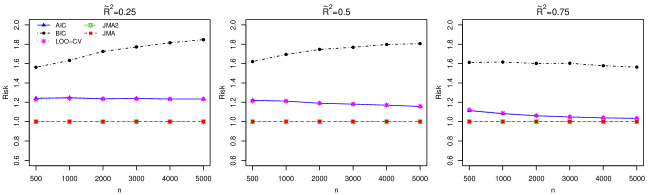
(a)

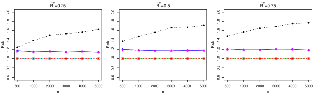
(b)

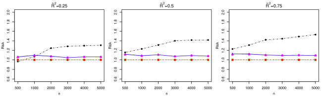
(c)

Figure 5: Simulation results for Example 2 with the case of slowly decaying $\theta_{m}^{*}$. Normalized risk functions for AIC, BIC, LOO-CV, JMA2, and JMA when $\theta_{m}^{*}=c^{2}m^{-2\alpha_{1}}$ with $\alpha_{1}=1$ in row (a), $\alpha_{1}=1.5$ in row (b), and $\alpha_{1}=2$ in row (c).

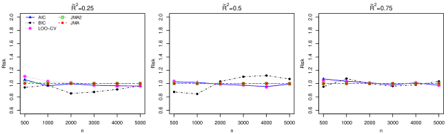
(a)

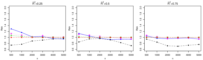
(b)

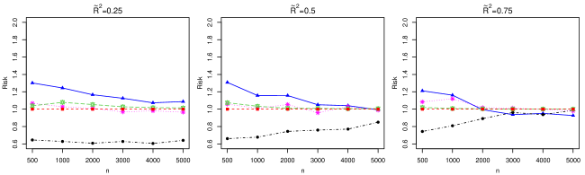
(c)

Figure 6: Simulation results for Example 2 with the case of fast decaying $\theta_{m}^{*}$. Normalized risk functions for AIC, BIC, LOO-CV, JMA2, and JMA when $\theta_{m}^{*}=c^{2}\exp(-2\alpha_{2}m)$ with $\alpha_{2}=1$ in row (a), $\alpha_{2}=1.5$ in row (b), and $\alpha_{2}=2$ in row (c).

Simulation results are shown in Figures 5–6. In each figure, the simulation results with three different decaying orders of $\theta_{m}^{*}$ are displayed in rows (a), (b), and (c), respectively. From these results, we see that in the slowly decaying $\theta_{m}^{*}$ case (Figure 5), the performance gap between LOO-CV and JMA does not vanish when sample size increases, while in the fast decaying $\theta_{m}^{*}$ case (Figure 6), it becomes very small when the sample size is large, which are consistent with the results of Corollary 1. Note that from Figure 6, the performances of AIC and JMA are not consistently close since AIC may not be asymptotically optimal in Example 2 because of heteroscedastisity. Another observation is that the performances of JMA2 and JMA are very close when $n$ is sufficiently large, which verify the results in Corollary 3. Moreover, we can observe the same phenomena as that in Example 1 for a comparison of AIC and BIC.

Example 3 (Non-orthonormal design) The setting of this example is the same as that of Example 1 except that the typical nested framework with $\nu_{m}=m$ and predictors are non-orthonormal. Specifically, the predictors $(x_{i1},\ldots,x_{ip_{n}})^{\top}$, $i=1,\ldots,n$, are iid normal random vectors with zero mean and covariance matrix between $k$th and $l$th elements being $\rho_{2}^{|k-l|}$, and the random errors $\varepsilon_{i}$ are iid from $N(0,\sigma^{2})$ and are independent of $x_{ij}$’s. Here, $\rho_{2}$ is set to be $0.5$. It is easy to prove that for any fixed $m$,

$${1\over n}\bm{\mu}^{\top}\mathbf{P}_{m}\bm{\mu}\xrightarrow{p}\lim_{n\to\infty}\bm{\beta}_{p_{n}}^{\top}\bm{\Sigma}_{m\times p_{n}}^{\top}\bm{\Sigma}_{m\times m}^{-1}\bm{\Sigma}_{m\times p_{n}}\bm{\beta}_{p_{n}},$$

where $\bm{\Sigma}_{d_{1}\times d_{2}}$ is a $d_{1}\times d_{2}$ matrix with $(k,l)$th element being $\rho_{2}^{|k-l|}$ and $\bm{\beta}_{p_{n}}=(\beta_{1},\ldots,\beta_{p_{n}})^{\top}$. It follows that $\theta_{n,m}=\bm{\mu}^{\top}(\mathbf{P}_{m}-\mathbf{P}_{m-1})\bm{\mu}/(n\sigma^{2})\to\theta_{m}^{*}=\xi_{m}/\sigma^{2}$ in probability, where $\xi_{1}=\lim_{n\to\infty}(\bm{\Sigma}_{1\times p_{n}}\bm{\beta}_{p_{n}})^{2}$ and

$$\xi_{m}=\lim_{n\to\infty}\bm{\beta}_{p_{n}}^{\top}\left\{\bm{\Sigma}_{m\times p_{n}}^{\top}\bm{\Sigma}_{m\times m}^{-1}\bm{\Sigma}_{m\times p_{n}}-\bm{\Sigma}_{(m-1)\times p_{n}}^{\top}\bm{\Sigma}_{(m-1)\times(m-1)}^{-1}\bm{\Sigma}_{(m-1)\times p_{n}}\right\}\bm{\beta}_{p_{n}}$$

for $m=2,\ldots,p_{n}$. By some calculations, we can obtain simple forms of $\xi_{m}$ as follows

$$\xi_{1}=\lim_{n\to\infty}\left(\sum_{j=1}^{p_{n}}\beta_{j}\rho_{2}^{j-1}\right)^{2},\quad\xi_{m}=\lim_{n\to\infty}(1-\rho_{2}^{2})\left(\sum_{j=m}^{p_{n}}\beta_{j}\rho_{2}^{j-m}\right)^{2},~{}m\geq 2.$$ (6.1)

We consider two cases with different decaying orders of $\theta_{m}^{*}$:

• Case 1 (With $\theta_{m}^{*}$ satisfying Condition B1). Here, $\xi_{m}=m^{-2\alpha_{1}}$ and $\alpha_{1}$ is set to be 1, 1.5 or 2.

• Case 2 (With $\theta_{m}^{*}$ satisfying Condition B2). Here, $\xi_{m}=\exp(-2\alpha_{2}m)$ and $\alpha_{2}$ is set to be 1, 1.5 or 2.

We can set different coefficient $\beta_{j}$ via (6.1) such that Case 1 and Case 2 hold respectively. Without loss of generality, we assume $\beta_{j}\geq 0$ for all $j$. Then from (6.1), we have

$$\beta_{1}=\sqrt{\xi_{1}}-\rho_{2}\sqrt{{\xi_{2}\over 1-\rho_{2}^{2}}}\quad\text{and}\quad\beta_{j}={\sqrt{\xi_{j}}-\rho_{2}\sqrt{\xi_{j+1}}\over\sqrt{1-\rho_{2}^{2}}},\quad j\geq 2.$$

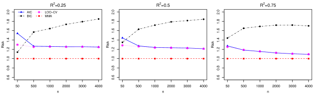
(a)

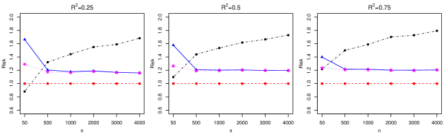
(b)

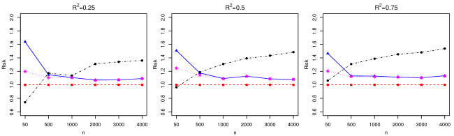
(c)

Figure 7: Simulation results for Example 3 with the case of slowly decaying $\theta_{m}^{*}$. Normalized risk functions for AIC, BIC, LOO-CV, and MMA when $\theta_{m}^{*}=m^{-2\alpha_{1}}/\sigma^{2}$ with $\alpha_{1}=1$ in row (a), $\alpha_{1}=1.5$ in row (b), and $\alpha_{1}=2$ in row (c).

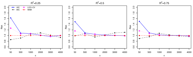
(a)

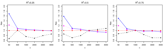
(b)

(c)

Figure 8: Simulation results for Example 3 with the case of fast decaying $\theta_{m}^{*}$. Normalized risk functions for AIC, BIC, LOO-CV, and MMA when $\theta_{m}^{*}=\exp(-2\alpha_{2}m)/\sigma^{2}$ with $\alpha_{2}=1$ in row (a), $\alpha_{2}=1.5$ in row (b), and $\alpha_{2}=2$ in row (c).

The sample size $n$ varies at 50, 500, 1000, 2000, 3000, and 4000. In each simulation setting of the combination of $n$, $R^{2}$, and $\alpha_{1}$ (or $\alpha_{2}$), we normalize the risks of the MS methods by dividing by the risk of MMA. Figures 7–8 display the simulation results for Case 1 and Case 2, respectively. In each figure, the simulation results with three different decaying orders of $\theta_{m}^{*}$ are displayed in rows (a), (b), and (c), respectively. From these results, we can see the same observations as that in Example 1, which also verify the previous theoretical findings.

In above examples, we use the decaying orders of GVI to determine the performance of MAs and MSs and set large enough $M_{n}$, i.e., (Condition M2 is satisfied). In Section of the Supplementary Material, we further design Example 4 to verify Corollary 1 when $M_{n}$ is too small (Condition M1 is satisfied).

7 Conclusion

This paper extends the work of Peng and Yang, (2021) on comparison of MS and MA to a general model setting, where we allow the predictors are non-orthonormal, the error terms are heteroscedastic and autocorrelated, and some predictors are totally unimportant. We obtain the results that the number of candidate models $M_{n}$ and the decaying order of $\{\theta_{n,m}\}_{m=1}^{d_{n}}$ determine when MA is better than MS. Specifically, when $M_{n}$ is large enough and $\theta_{n,m}$ decays slowly in $m$, the benefit of MA over MS is real; when $M_{n}$ is too small or $M_{n}$ is large enough and $\theta_{n,m}$ decays fast in $m$, the risks of MA and MS are asymptotically equivalent. Furthermore, the obtained results are extended to compare MAs with the weights belonged to three different weight sets.

Along with the paper, there are a few open questions. First, an interesting issue is how to order the predictors and prepare nested candidate models such that the risk gain of MA is optimal. Although various procedures are proposed to order the predictors in the implementation of MA such as forward selection approach (Claeskens et al.,, 2006), the marginal correlation (Ando and Li,, 2014, 2017; Zhang et al., 2016b, ), and solution path algorithm of penalized regression (Zhang et al.,, 2020; Feng and Liu,, 2020), there is still a lack of theoretical study on an optimal way of ordering the predictors. Second, it is interesting to develop a data-driven way to choose the number of the candidate models. Another appealing direction is to compare MS and MA in the non-nested model setting. However, in this case, it is difficult to characterize the unknown optimal model $m_{n}^{*}$ and weights $\bm{w}_{n}^{*}$. A deeper and detailed investigation of these issues warrants further studies.

Appendix

A.1 Proof of Theorem 1

The risk of the $m$th candidate model is

$$R_{n}(m) =E\|\widehat{\bm{\mu}}_{m}-\bm{\mu}\|^{2}$$

$$=\mathrm{tr}\left[E\left\{(\widehat{\bm{\mu}}_{m}-\bm{\mu})(\widehat{\bm{\mu}}_{m}-\bm{\mu})^{\top}\right\}\right]$$

$$=\mathrm{tr}\left\{(E\widehat{\bm{\mu}}_{m}-\bm{\mu})(E\widehat{\bm{\mu}}_{m}-\bm{\mu})^{\top}\right\}+\mathrm{tr}\left\{\mathrm{var}(\widehat{\bm{\mu}}_{m})\right\}$$

$$=\bm{\mu}^{\top}(\mathbf{I}_{n}-\mathbf{P}_{m})\bm{\mu}+\mathrm{tr}(\mathbf{P}_{m}\bm{\Omega}).$$

Observe that

$$R_{n}(m)-R_{n}(m-1)=\mathrm{tr}\{(\mathbf{P}_{m}-\mathbf{P}_{m-1})\bm{\Omega}\}-\bm{\mu}^{\top}(\mathbf{P}_{m}-\mathbf{P}_{m-1})\bm{\mu}=n\mathrm{tr}\{(\mathbf{P}_{m}-\mathbf{P}_{m-1})\bm{\Omega}\}\biggl{(}{1\over n}-\theta_{n,m}\biggr{)},$$ (A.1)

where $\theta_{n,m}$ is defined in (3.2). Note that $\mathrm{tr}\{(\mathbf{P}_{m}-\mathbf{P}_{m-1})\bm{\Omega}\}>0$ and $\{\theta_{n,m}\}_{m=1}^{q_{n}}$ is non-increasing from Assumption 3. Then, under Assumption 6, it is easy to see that the global optimal model $m_{n}^{**}$ that minimizes $R_{n}(m)$ on $\{1,\ldots,d_{n}\}$ satisfies

$$\theta_{n,m_{n}^{**}}>{1\over n}\geq\theta_{n,m_{n}^{**}+1}.$$ (A.2)

Hence, the risk of the optimal model $m_{n}^{*}$ is

$$R_{n}(m_{n}^{*})=\bm{\mu}^{\top}(\mathbf{I}_{n}-\mathbf{P}_{m_{n}^{*}})\bm{\mu}+\mathrm{tr}(\mathbf{P}_{m_{n}^{*}}\bm{\Omega}),$$ (A.3)

where when $M_{n}<m_{n}^{**}$, $m_{n}^{*}=M_{n}$ and $\theta_{n,m_{n}^{*}}>1/n$; when $M_{n}\geq m_{n}^{**}$, $m_{n}^{*}=m_{n}^{**}$ and

$$\theta_{n,m_{n}^{*}}>{1\over n}\geq\theta_{n,m_{n}^{*}+1}.$$ (A.4)

The risk of the MA estimator with weights $\bm{w}$ is

$$\begin{split}R_{n}(\bm{w})&=E\|\widehat{\bm{\mu}}(\bm{w})-\bm{\mu}\|^{2}=E\|\mathbf{P}(\bm{w})\bm{y}-\bm{\mu}\|^{2}\\ &=\bm{\mu}^{\top}\{\mathbf{P}(\bm{w})-\mathbf{I}_{n}\}^{2}\bm{\mu}+\mathrm{tr}\{\mathbf{P}^{2}(\bm{w})\bm{\Omega}\}.\end{split}$$

Rewrite $\mathbf{P}(\bm{w})=\sum_{m=1}^{M_{n}}\gamma_{m}(\mathbf{P}_{m}-\mathbf{P}_{m-1})$, where $\gamma_{m}=\sum_{j=m}^{M_{n}}w_{j}$ and $\mathbf{P}_{0}=\bm{0}$. Since $\mathbf{P}_{m}\mathbf{P}_{l}=\mathbf{P}_{\min(m,l)}$ for the nested candidate models, it is easy to verify that $\{\mathbf{P}_{m}-\mathbf{P}_{m-1}\}_{m=1}^{M_{n}}$ are mutually orthonormal projection matrices, i.e.,

$$(\mathbf{P}_{m_{1}}-\mathbf{P}_{m_{1}-1})(\mathbf{P}_{m_{2}}-\mathbf{P}_{m_{2}-1})=\begin{cases}\mathbf{P}_{m_{1}}-\mathbf{P}_{m_{1}-1},&\mathrm{if}~{}m_{1}=m_{2},\\ \mathbf{0},&\mathrm{if}~{}m_{1}\neq m_{2}.\end{cases}$$

Using the above fact, $R_{m}(\bm{w})$ is further expanded as

$$R_{n}(\bm{w})= \sum_{m=1}^{M_{n}}\biggl{(}\gamma_{m}^{2}\Bigl{[}\bm{\mu}^{\top}(\mathbf{P}_{m}-\mathbf{P}_{m-1})\bm{\mu}+\mathrm{tr}\{(\mathbf{P}_{m}-\mathbf{P}_{m-1})\bm{\Omega}\}\Bigr{]}$$ (A.5)

$$-2\gamma_{m}\bm{\mu}^{\top}(\mathbf{P}_{m}-\mathbf{P}_{m-1})\bm{\mu}+\bm{\mu}^{\top}(\mathbf{P}_{m}-\mathbf{P}_{m-1})\bm{\mu}\biggr{)}+\bm{\mu}^{\top}(\mathbf{I}_{n}-\mathbf{P}_{M_{n}})\bm{\mu}.$$

It is straightforward to show that the infeasible optimal weight $\bm{w}_{n}^{*}=(w_{n,1}^{*},\ldots,w_{n,M_{n}}^{*})^{\top}$ can be obtained by setting $w_{n,m}^{*}=\gamma_{n,m}^{*}-\gamma_{n,m+1}^{*}$ for $m=1,\ldots,M_{n}-1$ and $w_{n,M_{n}}^{*}=\gamma_{n,M_{n}}^{*}$, where $\gamma_{n,1}^{*}=1$ and

$$\gamma_{n,m}^{*}={\bm{\mu}^{\top}(\mathbf{P}_{m}-\mathbf{P}_{m-1})\bm{\mu}\over\bm{\mu}^{\top}(\mathbf{P}_{m}-\mathbf{P}_{m-1})\bm{\mu}+\mathrm{tr}\{(\mathbf{P}_{m}-\mathbf{P}_{m-1})\bm{\Omega}\}}={\theta_{n,m}\over\theta_{n,m}+1/n},\quad m=2,\ldots,M_{n}.$$ (A.6)

Hence, the risk of the optimal MA estimator is

$$R_{n}(\bm{w}_{n}^{*})=\mathrm{tr}(\mathbf{P}_{1}\bm{\Omega})+\sum_{m=2}^{M_{n}}{\mathrm{tr}\{(\mathbf{P}_{m}-\mathbf{P}_{m-1})\bm{\Omega}\}\bm{\mu}^{\top}(\mathbf{P}_{m}-\mathbf{P}_{m-1})\bm{\mu}\over\bm{\mu}^{\top}(\mathbf{P}_{m}-\mathbf{P}_{m-1})\bm{\mu}+\mathrm{tr}\{(\mathbf{P}_{m}-\mathbf{P}_{m-1})\bm{\Omega}\}}+\bm{\mu}^{\top}(\mathbf{I}_{n}-\mathbf{P}_{M_{n}})\bm{\mu}.$$ (A.7)

Combining (A.3) and (A.7), the potential advantage of MA over MS is

$$\Delta_{n} =R_{n}(m_{n}^{*})-R_{n}(\bm{w}_{n}^{*})$$ (A.8)

$$=\sum_{m=2}^{m_{n}^{*}}\biggl{[}\mathrm{tr}\{(\mathbf{P}_{m}-\mathbf{P}_{m-1})\bm{\Omega}\}-{\mathrm{tr}\{(\mathbf{P}_{m}-\mathbf{P}_{m-1})\bm{\Omega}\}\bm{\mu}^{\top}(\mathbf{P}_{m}-\mathbf{P}_{m-1})\bm{\mu}\over\bm{\mu}^{\top}(\mathbf{P}_{m}-\mathbf{P}_{m-1})\bm{\mu}+\mathrm{tr}\{(\mathbf{P}_{m}-\mathbf{P}_{m-1})\bm{\Omega}\}}\biggr{]}$$

$$\quad+\sum_{m=m_{n}^{*}+1}^{M_{n}}{\{\bm{\mu}^{\top}(\mathbf{P}_{m}-\mathbf{P}_{m-1})\bm{\mu}\}^{2}\over\bm{\mu}^{\top}(\mathbf{P}_{m}-\mathbf{P}_{m-1})\bm{\mu}+\mathrm{tr}\{(\mathbf{P}_{m}-\mathbf{P}_{m-1})\bm{\Omega}\}},$$

which implies that, as is expected, the optimal risk of MA is not larger than that of MS, i.e., $R_{n}(\bm{w}_{n}^{*})\leq R_{n}(m_{n}^{*})$. We consider two scenarios that $M_{n}<m_{n}^{**}$ and $M_{n}\geq m_{n}^{**}$.

When $M_{n}<m_{n}^{**}$, $m_{n}^{*}=M_{n}$ and it follows from Assumption 3 and $\theta_{n,m_{n}^{*}}>1/n$ that $\{\gamma_{n,m}^{*}\}_{m=1}^{M_{n}}$ is non-increasing and $\gamma_{n,m_{n}^{*}}^{*}>1/2$. Then, for a sufficiently large $n$,

$$R_{n}(\bm{w}_{n}^{*}) \geq\sum_{m=1}^{m_{n}^{*}}{\mathrm{tr}\{(\mathbf{P}_{m}-\mathbf{P}_{m-1})\bm{\Omega}\}\bm{\mu}^{\top}(\mathbf{P}_{m}-\mathbf{P}_{m-1})\bm{\mu}\over\bm{\mu}^{\top}(\mathbf{P}_{m}-\mathbf{P}_{m-1})\bm{\mu}+\mathrm{tr}\{(\mathbf{P}_{m}-\mathbf{P}_{m-1})\bm{\Omega}\}}+\bm{\mu}^{\top}(\mathbf{I}_{n}-\mathbf{P}_{m_{n}^{*}})\bm{\mu}$$

$$=\sum_{m=1}^{m_{n}^{*}}\gamma_{n,m}^{*}\mathrm{tr}\{(\mathbf{P}_{m}-\mathbf{P}_{m-1})\bm{\Omega}\}+\bm{\mu}^{\top}(\mathbf{I}_{n}-\mathbf{P}_{m_{n}^{*}})\bm{\mu}$$

$$\geq\gamma_{n,m_{n}^{*}}^{*}\sum_{m=1}^{m_{n}^{*}}\mathrm{tr}\{(\mathbf{P}_{m}-\mathbf{P}_{m-1})\bm{\Omega}\}+\bm{\mu}^{\top}(\mathbf{I}_{n}-\mathbf{P}_{m_{n}^{*}})\bm{\mu}$$

$$\geq{1\over 2}\mathrm{tr}(\mathbf{P}_{m_{n}^{*}}\bm{\Omega})+\bm{\mu}^{\top}(\mathbf{I}_{n}-\mathbf{P}_{m_{n}^{*}})\bm{\mu}\geq{1\over 2}R_{n}(m_{n}^{*}).$$

When $M_{n}\geq m_{n}^{**}$, it follows from Assumption 3 and (A.4) that $\gamma_{n,m_{n}^{*}}^{*}>1/2\geq\gamma_{n,m_{n}^{*}+1}^{*}$. Then, for a sufficiently large $n$,

$$R_{n}(\bm{w}_{n}^{*}) \geq\sum_{m=1}^{M_{n}}{\mathrm{tr}\{(\mathbf{P}_{m}-\mathbf{P}_{m-1})\bm{\Omega}\}\bm{\mu}^{\top}(\mathbf{P}_{m}-\mathbf{P}_{m-1})\bm{\mu}\over\bm{\mu}^{\top}(\mathbf{P}_{m}-\mathbf{P}_{m-1})\bm{\mu}+\mathrm{tr}\{(\mathbf{P}_{m}-\mathbf{P}_{m-1})\bm{\Omega}\}}+\bm{\mu}^{\top}(\mathbf{I}_{n}-\mathbf{P}_{M_{n}})\bm{\mu}$$

$$=\sum_{m=1}^{m_{n}^{*}}\gamma_{n,m}^{*}\mathrm{tr}\{(\mathbf{P}_{m}-\mathbf{P}_{m-1})\bm{\Omega}\}+\sum_{m=m_{n}^{*}+1}^{M_{n}}(1-\gamma_{n,m}^{*})\bm{\mu}^{\top}(\mathbf{P}_{m}-\mathbf{P}_{m-1})\bm{\mu}+\bm{\mu}^{\top}(\mathbf{I}_{n}-\mathbf{P}_{M_{n}})\bm{\mu}$$

$$\geq\gamma_{n,m_{n}^{*}}^{*}\sum_{m=1}^{m_{n}^{*}}\mathrm{tr}\{(\mathbf{P}_{m}-\mathbf{P}_{m-1})\bm{\Omega}\}+(1-\gamma_{n,m_{n}^{*}+1}^{*})\sum_{m=m_{n}^{*}+1}^{M_{n}}\bm{\mu}^{\top}(\mathbf{P}_{m}-\mathbf{P}_{m-1})\bm{\mu}+\bm{\mu}^{\top}(\mathbf{I}_{n}-\mathbf{P}_{M_{n}})\bm{\mu}$$

$$\geq{1\over 2}\mathrm{tr}(\mathbf{P}_{m_{n}^{*}}\bm{\Omega})+{1\over 2}\bm{\mu}^{\top}(\mathbf{P}_{M_{n}}-\mathbf{P}_{m_{n}^{*}})\bm{\mu}+\bm{\mu}^{\top}(\mathbf{I}_{n}-\mathbf{P}_{M_{n}})\bm{\mu}$$

$$\geq{1\over 2}R_{n}(m_{n}^{*}).$$

Therefore, we have $R_{n}(m_{n}^{*})\geq R_{n}(\bm{w}_{n}^{*})\geq R_{n}(m_{n}^{*})/2$ for any sufficiently large $n$, which yields that $R_{n}(m_{n}^{*})$ and $R_{n}(\bm{w}_{n}^{*})$ have the same order. This completes the proof of Theorem 1.

A.2 Proof of Theorem 2

We first prove (i). Let $C>0$ be a given sufficiently large constant. From Assumption 5, there exists a constant $K_{C}^{*}=\max\{K_{m},\lfloor 2/\bar{\theta}_{\lfloor C\rfloor+1}\rfloor+1\}>0$ such that $\theta_{n,\lfloor C\rfloor+1}-1/n\geq\bar{\theta}_{\lfloor C\rfloor+1}/2>0$ for any $n\geq K_{C}^{*}$. Since $m_{n}^{**}$ satisfies $1/n\geq\theta_{n,m_{n}^{**}+1}$ from (A.2), we have

$$\theta_{n,\lfloor C\rfloor+1}-\theta_{n,m_{n}^{**}+1}\geq\theta_{n,\lfloor C\rfloor+1}-{1\over n}>0,$$

which, along with Assumption 3, leads to $m_{n}^{**}+1\geq\lfloor C\rfloor+2$. This implies that for any constant $C>0$, there exists a constant $K_{C}^{*}>0$ such that $m_{n}^{**}\geq\lfloor C\rfloor+1>C$ for any $n\geq K_{C}^{*}$, i.e., $\lim_{n\to\infty}m_{n}^{**}=\infty$. This completes the proof of Theorem 2(i).

Next, we prove (ii). When $M_{n}\geq m_{n}^{**}$, $m_{n}^{*}=m_{n}^{**}$ and thus

$$R_{n}(m_{n}^{*})\geq\mathrm{tr}(\mathbf{P}_{m_{n}^{*}}\bm{\Omega})=\mathrm{tr}(\mathbf{P}_{m_{n}^{**}}\bm{\Omega})\geq c_{1}\nu_{m_{n}^{**}}\geq c_{1}m_{n}^{**}\to\infty.$$

When $M_{n}<m_{n}^{**}$, $m_{n}^{*}=M_{n}$ and thus by (A.2) and Assumptions 2–3,

$$R_{n}(m_{n}^{*}) =R_{n}(M_{n})=\bm{\mu}^{\top}(\mathbf{I}_{n}-\mathbf{P}_{M_{n}})\bm{\mu}+\mathrm{tr}(\mathbf{P}_{M_{n}}\bm{\Omega})$$ (A.9)

$$\geq\bm{\mu}^{\top}(\mathbf{P}_{m_{n}^{**}}-\mathbf{P}_{M_{n}})\bm{\mu}+\mathrm{tr}(\mathbf{P}_{M_{n}}\bm{\Omega})$$

$$=\sum_{m=M_{n}+1}^{m_{n}^{**}}\mathrm{tr}\{(\mathbf{P}_{m}-\mathbf{P}_{m-1})\bm{\Omega}\}n\theta_{n,m}+\mathrm{tr}(\mathbf{P}_{M_{n}}\bm{\Omega})$$

$$\geq n\theta_{n,m_{n}^{**}}\sum_{m=M_{n}+1}^{m_{n}^{**}}\mathrm{tr}\{(\mathbf{P}_{m}-\mathbf{P}_{m-1})\bm{\Omega}\}+\mathrm{tr}(\mathbf{P}_{M_{n}}\bm{\Omega})$$

$$\geq\mathrm{tr}\{(\mathbf{P}_{m_{n}^{**}}-\mathbf{P}_{M_{n}})\bm{\Omega}\}+\mathrm{tr}(\mathbf{P}_{M_{n}}\bm{\Omega})$$

$$=\mathrm{tr}(\mathbf{P}_{m_{n}^{**}}\bm{\Omega})\geq c_{1}\nu_{m_{n}^{**}}\geq c_{1}m_{n}^{**}\to\infty.$$

Therefore, $R_{n}(m_{n}^{*})\to\infty$ as $n\to\infty$ for any $M_{n}$. Combining it with Theorem 1, we have $R_{n}(\bm{w}_{n}^{*})\geq{1\over 2}R_{n}(m_{n}^{*})\to\infty$ as $n\to\infty$. This completes the proof of Theorem 2(ii).

A.3 Proof of Theorem 3

Under Condition M1, $\lim_{n\to\infty}M_{n}/m_{n}^{**}=0$, which implies that $M_{n}<m_{n}^{**}$ when $n$ is large enough and thus $m_{n}^{*}=M_{n}$. By (A.8), for a sufficiently large $n$,

$$\Delta_{n} =\sum_{m=2}^{M_{n}}{[\mathrm{tr}\{(\mathbf{P}_{m}-\mathbf{P}_{m-1})\bm{\Omega}\}]^{2}\over\bm{\mu}^{\top}(\mathbf{P}_{m}-\mathbf{P}_{m-1})\bm{\mu}+\mathrm{tr}\{(\mathbf{P}_{m}-\mathbf{P}_{m-1})\bm{\Omega}\}}$$ (A.10)

$$\leq\sum_{m=2}^{M_{n}}\mathrm{tr}\{(\mathbf{P}_{m}-\mathbf{P}_{m-1})\bm{\Omega}\}$$

$$=\mathrm{tr}\{(\mathbf{P}_{M_{n}}-\mathbf{P}_{1})\bm{\Omega}\}$$

$$\leq c_{2}(\nu_{M_{n}}-\nu_{1})\leq c_{2}V(M_{n}-1),$$

where the last two inequalities are due to Assumptions 2 and 4, respectively. Combining (A.9), (A.10), $\lim_{n\to\infty}M_{n}/m_{n}^{**}=0$, and Theorem 2, we have

$$\limsup_{n\to\infty}{\Delta_{n}\over R_{n}(m_{n}^{*})}\leq{c_{2}V\over c_{1}}\lim_{n\to\infty}{M_{n}-1\over m_{n}^{**}}=0,$$

which yields that $\Delta_{n}=o\{R_{n}(m_{n}^{*})\}$. This completes the proof of Theorem 3.

A.4 Proof of Theorem 4

When Condition M2 holds, we consider two scenarios: $M_{n}\geq m_{n}^{**}$ and $\underline{c}\leq M_{n}/m_{n}^{**}<1$ for any sufficiently large $n$, to prove this theorem.

(i) $M_{n}\geq m_{n}^{**}$ for any sufficiently large $n$. In this case, $m_{n}^{*}=m_{n}^{**}$ satisfies (A.4). When Condition A1 holds, we first examine the order of the optimal risk of MS. Let $s_{n}^{*}=\max\{s:\lfloor k^{s}(m_{n}^{*}+1)\rfloor\leq d_{n},s=0,1,\ldots\}$. The first term in (A.3) is upper bounded by

$$\bm{\mu}^{\top}(\mathbf{I}_{n}-\mathbf{P}_{m_{n}^{*}})\bm{\mu}$$

$$\quad=\sum_{m=m_{n}^{*}+1}^{q_{n}}\bm{\mu}^{\top}(\mathbf{P}_{m}-\mathbf{P}_{m-1})\bm{\mu}=\sum_{m=m_{n}^{*}+1}^{d_{n}}\bm{\mu}^{\top}(\mathbf{P}_{m}-\mathbf{P}_{m-1})\bm{\mu}$$

$$\quad=\sum_{s=0}^{s_{n}^{*}-1}\sum_{m=\lfloor k^{s}(m_{n}^{*}+1)\rfloor}^{\lfloor k^{s+1}(m_{n}^{*}+1)\rfloor-1}\bm{\mu}^{\top}(\mathbf{P}_{m}-\mathbf{P}_{m-1})\bm{\mu}+\sum_{m=\lfloor k^{s_{n}^{*}}(m_{n}^{*}+1)\rfloor}^{d_{n}}\bm{\mu}^{\top}(\mathbf{P}_{m}-\mathbf{P}_{m-1})\bm{\mu}$$

$$\quad=\sum_{s=0}^{s_{n}^{*}-1}\sum_{m=\lfloor k^{s}(m_{n}^{*}+1)\rfloor}^{\lfloor k^{s+1}(m_{n}^{*}+1)\rfloor-1}n\mathrm{tr}\{(\mathbf{P}_{m}-\mathbf{P}_{m-1})\bm{\Omega}\}\theta_{n,m}+\sum_{m=\lfloor k^{s_{n}^{*}}(m_{n}^{*}+1)\rfloor}^{d_{n}}n\mathrm{tr}\{(\mathbf{P}_{m}-\mathbf{P}_{m-1})\bm{\Omega}\}\theta_{n,m}$$

$$\quad\leq\sum_{s=0}^{s_{n}^{*}-1}\theta_{n,\lfloor k^{s}(m_{n}^{*}+1)\rfloor}\sum_{m=\lfloor k^{s}(m_{n}^{*}+1)\rfloor}^{\lfloor k^{s+1}(m_{n}^{*}+1)\rfloor-1}n\mathrm{tr}\{(\mathbf{P}_{m}-\mathbf{P}_{m-1})\bm{\Omega}\}$$

$$\qquad+\theta_{n,\lfloor k^{s_{n}^{*}}(m_{n}^{*}+1)\rfloor}\sum_{m=\lfloor k^{s_{n}^{*}}(m_{n}^{*}+1)\rfloor}^{d_{n}}n\mathrm{tr}\{(\mathbf{P}_{m}-\mathbf{P}_{m-1})\bm{\Omega}\}$$

$$\quad\leq n\theta_{n,m_{n}^{*}+1}\sum_{s=0}^{s_{n}^{*}-1}\eta^{s}\mathrm{tr}\{(\mathbf{P}_{\lfloor k^{s+1}(m_{n}^{*}+1)\rfloor-1}-\mathbf{P}_{\lfloor k^{s}(m_{n}^{*}+1)\rfloor-1})\bm{\Omega}\}$$

$$\qquad+n\theta_{n,m_{n}^{*}+1}\eta^{s_{n}^{*}}\mathrm{tr}\{(\mathbf{P}_{d_{n}}-\mathbf{P}_{\lfloor k^{s_{n}^{*}}(m_{n}^{*}+1)\rfloor-1})\bm{\Omega}\}$$

$$\quad\leq c_{2}\sum_{s=0}^{s_{n}^{*}-1}\eta^{s}(\nu_{\lfloor k^{s+1}(m_{n}^{*}+1)\rfloor}-\nu_{\lfloor k^{s}(m_{n}^{*}+1)\rfloor})+c_{2}\eta^{s_{n}^{*}}(\nu_{d_{n}}-\nu_{\lfloor k^{s_{n}^{*}}(m_{n}^{*}+1)\rfloor-1})$$

$$\quad\leq c_{2}V\sum_{s=0}^{s_{n}^{*}}\eta^{s}(\lfloor k^{s+1}(m_{n}^{*}+1)\rfloor-\lfloor k^{s}(m_{n}^{*}+1)\rfloor)$$

$$\quad\sim c_{2}V(k-1)(m_{n}^{*}+1)\sum_{s=0}^{s_{n}^{*}}(k\eta)^{s}\asymp m_{n}^{*}\asymp\mathrm{tr}(\mathbf{P}_{m_{n}^{*}}\bm{\Omega}),$$

where the first equality follows from the fact that $\bm{\mu}^{\top}(\mathbf{I}_{n}-\mathbf{P}_{q_{n}})\bm{\mu}=0$, the first inequality follows from Assumption 3, the second inequality follows from $\theta_{n,\lfloor k^{s}(m_{n}^{*}+1)\rfloor}/\theta_{n,m_{n}^{*}+1}\leq\eta^{s}$ for a sufficiently large $n$, which can be obtained by Condition A1 and Theorem 2, and the last two inequalities follow from (A.4) and Assumption 4 respectively. Thus, the order of the optimal risk of MS satisfies $R_{n}(m_{n}^{*})\asymp\mathrm{tr}(\mathbf{P}_{m_{n}^{*}}\bm{\Omega})$.

Next, we prove that the potential advantage $\Delta_{n}$ of MA over MS has the same order as $R_{n}(m_{n}^{*})$ under Condition A1. Define $t_{n}=\min\{t\in\mathbb{N}:\lfloor kt\rfloor\geq m_{n}^{*}+1\}$. Then it follows from Theorem 2 and Peng and Yang, (2021) that $\lim_{n\to\infty}t_{n}=\infty$, $\lfloor kt_{n}\rfloor\sim m_{n}^{*}$, and $t_{n}\sim m_{n}^{*}/k$. The first term in (A.8) can be lower bounded by

$$\sum_{m=2}^{m_{n}^{*}}\biggl{[}\mathrm{tr}\{(\mathbf{P}_{m}-\mathbf{P}_{m-1})\bm{\Omega}\}-{\mathrm{tr}\{(\mathbf{P}_{m}-\mathbf{P}_{m-1})\bm{\Omega}\}\bm{\mu}^{\top}(\mathbf{P}_{m}-\mathbf{P}_{m-1})\bm{\mu}\over\bm{\mu}^{\top}(\mathbf{P}_{m}-\mathbf{P}_{m-1})\bm{\mu}+\mathrm{tr}\{(\mathbf{P}_{m}-\mathbf{P}_{m-1})\bm{\Omega}\}}\biggr{]}$$

$$\quad\geq\mathrm{tr}\{(\mathbf{P}_{m_{n}^{*}}-\mathbf{P}_{1})\bm{\Omega}\}-\sum_{m=2}^{\lfloor kt_{n}\rfloor}{\mathrm{tr}\{(\mathbf{P}_{m}-\mathbf{P}_{m-1})\bm{\Omega}\}\bm{\mu}^{\top}(\mathbf{P}_{m}-\mathbf{P}_{m-1})\bm{\mu}\over\bm{\mu}^{\top}(\mathbf{P}_{m}-\mathbf{P}_{m-1})\bm{\mu}+\mathrm{tr}\{(\mathbf{P}_{m}-\mathbf{P}_{m-1})\bm{\Omega}\}}$$

$$\quad\geq\mathrm{tr}\{(\mathbf{P}_{m_{n}^{*}}-\mathbf{P}_{1})\bm{\Omega}\}-\sum_{m=2}^{t_{n}}\mathrm{tr}\{(\mathbf{P}_{m}-\mathbf{P}_{m-1})\bm{\Omega}\}-\sum_{m=t_{n}+1}^{\lfloor kt_{n}\rfloor}{\mathrm{tr}\{(\mathbf{P}_{m}-\mathbf{P}_{m-1})\bm{\Omega}\}\over 1+1/(n\theta_{n,m})}$$

$$\quad\geq\mathrm{tr}\{(\mathbf{P}_{m_{n}^{*}}-\mathbf{P}_{t_{n}})\bm{\Omega}\}-{1\over 1+1/(n\theta_{n,t_{n}})}\mathrm{tr}\{(\mathbf{P}_{\lfloor kt_{n}\rfloor}-\mathbf{P}_{t_{n}})\bm{\Omega}\},$$

$$\quad\geq\mathrm{tr}\{(\mathbf{P}_{m_{n}^{*}}-\mathbf{P}_{t_{n}})\bm{\Omega}\}-{1\over 1+\delta}\mathrm{tr}\{(\mathbf{P}_{\lfloor kt_{n}\rfloor}-\mathbf{P}_{t_{n}})\bm{\Omega}\}$$

$$\quad={1\over 1+\delta}\mathrm{tr}\big{[}\{(1+\delta)\mathbf{P}_{m_{n}^{*}}-\mathbf{P}_{\lfloor kt_{n}\rfloor}-\delta\mathbf{P}_{t_{n}}\}\bm{\Omega}\bigr{]}$$ (A.11)

where the third inequality follows from Assumption 3 and the last inequality follows from the following fact

$${1\over 1+1/(n\theta_{n,t_{n}})}\leq{1\over 1+\delta/(n\theta_{n,\lfloor kt_{n}\rfloor})}\leq{1\over 1+\delta/(n\theta_{n,m_{n}^{*}+1})}\leq{1\over 1+\delta},$$

which can be derived by (A.4) and Condition A1. Since $\nu_{m_{n}^{*}}\sim\nu_{\lfloor kt_{n}\rfloor}$, it is easy to show that $(1+\delta)\mathbf{P}_{m_{n}^{*}}-\mathbf{P}_{\lfloor kt_{n}\rfloor}-\delta\mathbf{P}_{t_{n}}$ is positive semi-definite for sufficiently large $n$. By Assumption 2 and the fact that $\mathrm{tr}(\mathbf{A}\mathbf{B})\geq\lambda_{\min}(\mathbf{A})\mathrm{tr}(\mathbf{B})$ for symmetric matrix $\mathbf{A}$ and positive semi-definite matrix $\mathbf{B}$ (Bernstein,, 2005, Proposition 8.4.13), we have

$${1\over 1+\delta}\mathrm{tr}\big{[}\{(1+\delta)\mathbf{P}_{m_{n}^{*}}-\mathbf{P}_{\lfloor kt_{n}\rfloor}-\delta\mathbf{P}_{t_{n}}\}\bm{\Omega}\bigr{]}$$

$$\quad\geq{c_{1}\over 1+\delta}\{(1+\delta)\nu_{m_{n}^{*}}-\nu_{\lfloor kt_{n}\rfloor}-\delta\nu_{t_{n}}\}$$

$$\quad\geq{c_{1}\over 1+\delta}(\nu_{m_{n}^{*}}-\nu_{\lfloor kt_{n}\rfloor})+{c_{1}\delta\over 1+\delta}(m_{n}^{*}-t_{n})$$

$$\quad\sim{(k-1)c_{1}\delta\over k(1+\delta)}m_{n}^{*}\asymp\mathrm{tr}(\mathbf{P}_{m_{n}^{*}}\bm{\Omega}),$$ (A.12)

where the last line is due to $\nu_{m_{n}^{*}}\sim\nu_{\lfloor kt_{n}\rfloor}$ and $t_{n}\sim m_{n}^{*}/k$. From (A.8), we see

$$R_{n}(m_{n}^{*})\geq\Delta_{n}\geq\sum_{m=2}^{m_{n}^{*}}\biggl{[}\mathrm{tr}\{(\mathbf{P}_{m}-\mathbf{P}_{m-1})\bm{\Omega}\}-{\mathrm{tr}\{(\mathbf{P}_{m}-\mathbf{P}_{m-1})\bm{\Omega}\}\bm{\mu}^{\top}(\mathbf{P}_{m}-\mathbf{P}_{m-1})\bm{\mu}\over\bm{\mu}^{\top}(\mathbf{P}_{m}-\mathbf{P}_{m-1})\bm{\mu}+\mathrm{tr}\{(\mathbf{P}_{m}-\mathbf{P}_{m-1})\bm{\Omega}\}}\biggr{]},$$

which, along with (A.4) and (A.4), implies $\Delta_{n}\asymp R_{n}(m_{n}^{*})$. This completes the proof of the result under Condition A1.

When Condition A2 holds, we next examine $\Delta_{n}=o\{R_{n}(m_{n}^{*})\}$. Let $2/m_{n}^{*}<k^{\prime}<1$. The first term in (A.8) is upper bounded by

$$\sum_{m=2}^{m_{n}^{*}}\biggl{[}\mathrm{tr}\{(\mathbf{P}_{m}-\mathbf{P}_{m-1})\bm{\Omega}\}-{\mathrm{tr}\{(\mathbf{P}_{m}-\mathbf{P}_{m-1})\bm{\Omega}\}\bm{\mu}^{\top}(\mathbf{P}_{m}-\mathbf{P}_{m-1})\bm{\mu}\over\bm{\mu}^{\top}(\mathbf{P}_{m}-\mathbf{P}_{m-1})\bm{\mu}+\mathrm{tr}\{(\mathbf{P}_{m}-\mathbf{P}_{m-1})\bm{\Omega}\}}\biggr{]}$$

$$\quad\leq\mathrm{tr}\{(\mathbf{P}_{m_{n}^{*}}-\mathbf{P}_{1})\bm{\Omega}\}-\sum_{m=2}^{\lfloor k^{\prime}m_{n}^{*}\rfloor}{\mathrm{tr}\{(\mathbf{P}_{m}-\mathbf{P}_{m-1})\bm{\Omega}\}\over 1+1/(n\theta_{n,m})}$$

$$\quad\leq\mathrm{tr}\{(\mathbf{P}_{m_{n}^{*}}-\mathbf{P}_{1})\bm{\Omega}\}-{1\over 1+1/(n\theta_{n,\lfloor k^{\prime}m_{n}^{*}\rfloor})}\sum_{m=2}^{\lfloor k^{\prime}m_{n}^{*}\rfloor}\mathrm{tr}\{(\mathbf{P}_{m}-\mathbf{P}_{m-1})\bm{\Omega}\}$$

$$\quad=\mathrm{tr}\{(\mathbf{P}_{m_{n}^{*}}-\mathbf{P}_{1})\bm{\Omega}\}-{1\over 1+1/(n\theta_{n,\lfloor k^{\prime}m_{n}^{*}\rfloor})}\mathrm{tr}\{(\mathbf{P}_{\lfloor k^{\prime}m_{n}^{*}\rfloor}-\mathbf{P}_{1})\bm{\Omega}\}$$

$$\quad=\mathrm{tr}\biggl{\{}\biggl{(}\mathbf{P}_{m_{n}^{*}}-\mathbf{P}_{1}-{\mathbf{P}_{\lfloor k^{\prime}m_{n}^{*}\rfloor}-\mathbf{P}_{1}\over 1+1/(n\theta_{n,\lfloor k^{\prime}m_{n}^{*}\rfloor})}\biggr{)}\bm{\Omega}\biggr{\}}.$$ (A.13)

Observe that

$$\mathbf{P}_{m_{n}^{*}}-\mathbf{P}_{1}-{\mathbf{P}_{\lfloor k^{\prime}m_{n}^{*}\rfloor}-\mathbf{P}_{1}\over 1+1/(n\theta_{n,\lfloor k^{\prime}m_{n}^{*}\rfloor})}={\mathbf{P}_{m_{n}^{*}}-\mathbf{P}_{\lfloor k^{\prime}m_{n}^{*}\rfloor}+(\mathbf{P}_{m_{n}^{*}}-\mathbf{P}_{1})/(n\theta_{n,\lfloor k^{\prime}m_{n}^{*}\rfloor})\over 1+1/(n\theta_{n,\lfloor k^{\prime}m_{n}^{*}\rfloor})}$$

is a positive semi-definite matrix. By the fact that $\mathrm{tr}(\mathbf{A}\mathbf{B})\leq\lambda_{\max}(\mathbf{A})\mathrm{tr}(\mathbf{B})$ for symmetric matrix $\mathbf{A}$ and positive semi-definite matrix $\mathbf{B}$ (Bernstein,, 2005, Proposition 8.4.13), we have

$$\mathrm{tr}\biggl{\{}\biggl{(}\mathbf{P}_{m_{n}^{*}}-\mathbf{P}_{1}-{\mathbf{P}_{\lfloor k^{\prime}m_{n}^{*}\rfloor}-\mathbf{P}_{1}\over 1+1/(n\theta_{n,\lfloor k^{\prime}m_{n}^{*}\rfloor})}\biggr{)}\bm{\Omega}\biggr{\}}$$

$$\quad\leq{c_{2}\over 1+1/(n\theta_{n,\lfloor k^{\prime}m_{n}^{*}\rfloor})}\mathrm{tr}\biggl{(}\mathbf{P}_{m_{n}^{*}}-\mathbf{P}_{\lfloor k^{\prime}m_{n}^{*}\rfloor}+{\mathbf{P}_{m_{n}^{*}}-\mathbf{P}_{1}\over n\theta_{n,\lfloor k^{\prime}m_{n}^{*}\rfloor}}\biggr{)}$$

$$\quad={c_{2}\over 1+1/(n\theta_{n,\lfloor k^{\prime}m_{n}^{*}\rfloor})}\biggl{(}\nu_{m_{n}^{*}}-\nu_{\lfloor k^{\prime}m_{n}^{*}\rfloor}+{\nu_{m_{n}^{*}}-\nu_{1}\over n\theta_{n,\lfloor k^{\prime}m_{n}^{*}\rfloor}}\biggr{)}$$

$$\quad\leq{c_{2}V\over 1+1/(n\theta_{n,\lfloor k^{\prime}m_{n}^{*}\rfloor})}\biggl{(}m_{n}^{*}-\lfloor k^{\prime}m_{n}^{*}\rfloor+{m_{n}^{*}-1\over n\theta_{n,\lfloor k^{\prime}m_{n}^{*}\rfloor}}\biggr{)}$$

$$\quad\leq c_{2}V\biggl{\{}m_{n}^{*}-\lfloor k^{\prime}m_{n}^{*}\rfloor+{\theta_{n,m_{n}^{*}}\over\theta_{n,\lfloor k^{\prime}m_{n}^{*}\rfloor}}(m_{n}^{*}-1)\biggr{\}},$$ (A.14)

where the second inequality follows from Assumption 4. Since $\lim_{n\to\infty}\theta_{n,m_{n}^{*}}/\theta_{n,\lfloor k^{\prime}m_{n}^{*}\rfloor}=0$ for any $k^{\prime}<1$ under Condition A2 and Theorem 2, we have

$$\biggl{\{}m_{n}^{*}-\lfloor k^{\prime}m_{n}^{*}\rfloor+{\theta_{n,m_{n}^{*}}\over\theta_{n,\lfloor k^{\prime}m_{n}^{*}\rfloor}}(m_{n}^{*}-1)\biggr{\}}\Big{/}m_{n}^{*}=1-{\lfloor k^{\prime}m_{n}^{*}\rfloor\over m_{n}^{*}}+{\theta_{n,m_{n}^{*}}\over\theta_{n,\lfloor k^{\prime}m_{n}^{*}\rfloor}}\left(1-{1\over m_{n}^{*}}\right)\to 1-k^{\prime},$$

which, along with (A.4) and (A.4), yields that

$$\sum_{m=2}^{m_{n}^{*}}\biggl{[}\mathrm{tr}\{(\mathbf{P}_{m}-\mathbf{P}_{m-1})\bm{\Omega}\}-{\mathrm{tr}\{(\mathbf{P}_{m}-\mathbf{P}_{m-1})\bm{\Omega}\}\bm{\mu}^{\top}(\mathbf{P}_{m}-\mathbf{P}_{m-1})\bm{\mu}\over\bm{\mu}^{\top}(\mathbf{P}_{m}-\mathbf{P}_{m-1})\bm{\mu}+\mathrm{tr}\{(\mathbf{P}_{m}-\mathbf{P}_{m-1})\bm{\Omega}\}}\biggr{]}=O\{(1-k^{\prime})m_{n}^{*}\}.$$

Due to the arbitrariness of $k^{\prime}$ and the fact $\mathrm{tr}(\mathbf{P}_{m_{n}^{*}}\bm{\Omega})\asymp m_{n}^{*}$, letting $k^{\prime}\to 1$, we can obtain the first term of (A.8):

$$\sum_{m=2}^{m_{n}^{*}}\biggl{[}\mathrm{tr}\{(\mathbf{P}_{m}-\mathbf{P}_{m-1})\bm{\Omega}\}-{\mathrm{tr}\{(\mathbf{P}_{m}-\mathbf{P}_{m-1})\bm{\Omega}\}\bm{\mu}^{\top}(\mathbf{P}_{m}-\mathbf{P}_{m-1})\bm{\mu}\over\bm{\mu}^{\top}(\mathbf{P}_{m}-\mathbf{P}_{m-1})\bm{\mu}+\mathrm{tr}\{(\mathbf{P}_{m}-\mathbf{P}_{m-1})\bm{\Omega}\}}\biggr{]}=o\{\mathrm{tr}(\mathbf{P}_{m_{n}^{*}}\bm{\Omega})\}.$$ (A.15)

Next, we consider the order of the second term of (A.8). Choose $k>1$. We have

$$\begin{split}&\sum_{m=m_{n}^{*}+1}^{M_{n}}{\{\bm{\mu}^{\top}(\mathbf{P}_{m}-\mathbf{P}_{m-1})\bm{\mu}\}^{2}\over\bm{\mu}^{\top}(\mathbf{P}_{m}-\mathbf{P}_{m-1})\bm{\mu}+\mathrm{tr}\{(\mathbf{P}_{m}-\mathbf{P}_{m-1})\bm{\Omega}\}}\\ &\quad=\sum_{m=m_{n}^{*}+1}^{\lfloor k(m_{n}^{*}+1)\rfloor}{n\theta_{n,m}\over 1+1/(n\theta_{n,m})}\mathrm{tr}\{(\mathbf{P}_{m}-\mathbf{P}_{m-1})\bm{\Omega}\}+\sum_{m=\lfloor k(m_{n}^{*}+1)\rfloor+1}^{\min\{M_{n},d_{n}\}}{\bm{\mu}^{\top}(\mathbf{P}_{m}-\mathbf{P}_{m-1})\bm{\mu}\over 1+1/(n\theta_{n,m})}.\end{split}$$ (A.16)

The first term of (A.16) is upper bounded by

$$\sum_{m=m_{n}^{*}+1}^{\lfloor k(m_{n}^{*}+1)\rfloor}{n\theta_{n,m}\over 1+1/(n\theta_{n,m})}\mathrm{tr}\{(\mathbf{P}_{m}-\mathbf{P}_{m-1})\bm{\Omega}\}$$

$$\quad\leq{n\theta_{n,m_{n}*+1}\over 1+1/(n\theta_{n,m_{n}^{*}+1})}\sum_{m=m_{n}^{*}+1}^{\lfloor k(m_{n}^{*}+1)\rfloor}\mathrm{tr}\{(\mathbf{P}_{m}-\mathbf{P}_{m-1})\bm{\Omega}\}$$

$$\quad\leq{1\over 2}\mathrm{tr}\{(\mathbf{P}_{\lfloor k(m_{n}^{*}+1)\rfloor}-\mathbf{P}_{m_{n}^{*}})\bm{\Omega}\}$$

$$\quad\leq{c_{2}\over 2}(\nu_{\lfloor k(m_{n}^{*}+1)\rfloor}-\nu_{m_{n}^{*}})$$

$$\quad\leq{c_{2}\over 2}V(\lfloor k(m_{n}^{*}+1)\rfloor-m_{n}^{*}),$$

where the first two inequalities follow from Assumption 3 and (A.4), respectively, and the last inequality follows from Assumption 4. Using Theorem 2, as $n\to\infty$,

$${\lfloor k(m_{n}^{*}+1)\rfloor-m_{n}^{*}\over m_{n}^{*}}={\lfloor k(m_{n}^{*}+1)\rfloor\over m_{n}^{*}}-1\to k-1.$$

Therefore,

$$\sum_{m=m_{n}^{*}+1}^{\lfloor k(m_{n}^{*}+1)\rfloor}{n\theta_{n,m}\over 1+1/(n\theta_{n,m})}\mathrm{tr}\{(\mathbf{P}_{m}-\mathbf{P}_{m-1})\bm{\Omega}\}=O\{(k-1)m_{n}^{*}\}=O\{(k-1)\mathrm{tr}(\mathbf{P}_{m_{n}^{*}}\bm{\Omega})\}.$$ (A.17)

The second term of (A.16) can be upper bounded by

$$\sum_{m=\lfloor k(m_{n}^{*}+1)\rfloor+1}^{\min\{M_{n},d_{n}\}}{\bm{\mu}^{\top}(\mathbf{P}_{m}-\mathbf{P}_{m-1})\bm{\mu}\over 1+1/(n\theta_{n,m})}$$

$$\quad\leq{1\over 1+1/(n\theta_{n,\lfloor k(m_{n}^{*}+1)\rfloor})}\sum_{m=\lfloor k(m_{n}^{*}+1)\rfloor+1}^{\min\{M_{n},d_{n}\}}\bm{\mu}^{\top}(\mathbf{P}_{m}-\mathbf{P}_{m-1})\bm{\mu}$$

$$\quad\leq{1\over 1+\theta_{n,m_{n}^{*}+1}/\theta_{n,\lfloor k(m_{n}^{*}+1)\rfloor}}\bm{\mu}^{\top}(\mathbf{P}_{\min\{M_{n},d_{n}\}}-\mathbf{P}_{\lfloor k(m_{n}^{*}+1)\rfloor})\bm{\mu}$$

$$\quad\leq{1\over 1+\theta_{n,m_{n}^{*}+1}/\theta_{n,\lfloor k(m_{n}^{*}+1)\rfloor}}\bm{\mu}^{\top}(\mathbf{I}_{n}-\mathbf{P}_{m_{n}^{*}})\bm{\mu}$$

$$\quad=o\{\bm{\mu}^{\top}(\mathbf{I}_{n}-\mathbf{P}_{m_{n}^{*}})\bm{\mu}\},$$ (A.18)

where the first two inequalities follow from Assumption 3 and (A.4), respectively, the last inequality follows from the following fact

$$\bm{\mu}^{\top}(\mathbf{I}_{n}-\mathbf{P}_{m_{n}^{*}})\bm{\mu}= \bm{\mu}^{\top}(\mathbf{I}_{n}-\mathbf{P}_{\min\{M_{n},d_{n}\}})\bm{\mu}+\bm{\mu}^{\top}(\mathbf{P}_{\min\{M_{n},d_{n}\}}-\mathbf{P}_{\lfloor k(m_{n}^{*}+1)\rfloor})\bm{\mu}$$

$$+\bm{\mu}^{\top}(\mathbf{P}_{\lfloor k(m_{n}^{*}+1)\rfloor}-\mathbf{P}_{m_{n}^{*}})\bm{\mu}$$

$$\geq \bm{\mu}^{\top}(\mathbf{P}_{\min\{M_{n},d_{n}\}}-\mathbf{P}_{\lfloor k(m_{n}^{*}+1)\rfloor})\bm{\mu},$$

and the last equality follows from the fact that $\lim_{n\to\infty}\theta_{n,\lfloor k(m_{n}^{*}+1)\rfloor}/\theta_{n,m_{n}^{*}+1}=0$ for any $k>1$ under Condition A2. Combining (A.16), (A.17), and (A.18), we have

$$\sum_{m=m_{n}^{*}+1}^{M_{n}}{\{\bm{\mu}^{\top}(\mathbf{P}_{m}-\mathbf{P}_{m-1})\bm{\mu}\}^{2}\over\bm{\mu}^{\top}(\mathbf{P}_{m}-\mathbf{P}_{m-1})\bm{\mu}+\mathrm{tr}\{(\mathbf{P}_{m}-\mathbf{P}_{m-1})\bm{\Omega}\}}=O\{(k-1)\mathrm{tr}(\mathbf{P}_{m_{n}^{*}}\bm{\Omega})\}+o\{\bm{\mu}^{\top}(\mathbf{I}_{n}-\mathbf{P}_{m_{n}^{*}})\bm{\mu}\}.$$

Duo to the arbitrariness of $k$, letting $k\to 1$, we have

$$\sum_{m=m_{n}^{*}+1}^{M_{n}}{\{\bm{\mu}^{\top}(\mathbf{P}_{m}-\mathbf{P}_{m-1})\bm{\mu}\}^{2}\over\bm{\mu}^{\top}(\mathbf{P}_{m}-\mathbf{P}_{m-1})\bm{\mu}+\mathrm{tr}\{(\mathbf{P}_{m}-\mathbf{P}_{m-1})\bm{\Omega}\}}=o\{R_{n}(m_{n}^{*})\},$$

which, along with (A.8) and (A.15), leads to $\Delta_{n}=o\{R_{n}(m_{n}^{*})\}$. This completes the proof of the result under Condition A2.

(ii) $\underline{c}\leq M_{n}/m_{n}^{**}<1$ for any sufficiently large $n$. In this case, $m_{n}^{*}=M_{n}\asymp m_{n}^{**}$. When Condition A1 holds, there exists a finite positive integer $\tau_{1}$ such that $k^{-\tau_{1}}\leq\underline{c}$. Therefore,

$$\theta_{n,m_{n}^{*}+1}=\theta_{n,M_{n}+1}\leq\theta_{n,\lfloor\underline{c}m_{n}^{**}\rfloor+1}\leq\theta_{n,\lfloor k^{-\tau_{1}}(m_{n}^{**}+1)\rfloor}\leq\delta^{-\tau_{1}}\theta_{n,m_{n}^{**}+1}\leq\delta^{-\tau_{1}}{1\over n},$$ (A.19)

where the last inequality is due to (A.2). Then, using the same arguments in (i) and (A.19), it is easy to prove the result under Condition A1. When Condition A2 holds, we can also obtain (A.15), which, along with the fact that the second term of (A.8) equals 0, yields the result under Condition A2. This completes the proof of Theorem 4 under (ii).

A.5 Proof of Lemma 1

From Assumption 7, we know that for any small $0<\epsilon<1$, there exists a constant $K_{\epsilon}>0$ which does not depend on $m$, such that $0<1-\epsilon\leq\theta_{n,m}/\theta_{m}^{*}\leq 1+\epsilon$ holds uniformly in $m=1,\ldots,d_{n}$ and $n\geq K_{\epsilon}$.

(i) When Condition B1 holds, there exist constants $k>1$ and $0<\delta^{*}\leq\eta^{*}<1$ with $k\eta^{*}<1$ such that for a sufficiently large $n$,

$${1-\epsilon\over 1+\epsilon}\delta^{*}\leq{\theta_{n,\lfloor kl_{n}\rfloor}\over\theta_{n,l_{n}}}={\theta_{n,\lfloor kl_{n}\rfloor}\over\theta_{\lfloor kl_{n}\rfloor}^{*}}\times{\theta_{\lfloor kl_{n}\rfloor}^{*}\over\theta_{l_{n}}^{*}}\times{\theta_{l_{n}}^{*}\over\theta_{n,l_{n}}}\leq{1+\epsilon\over 1-\epsilon}\eta^{*}.$$

Let $\delta={1-\epsilon\over 1+\epsilon}\delta^{*}$ and $\eta={1+\epsilon\over 1-\epsilon}\eta^{*}$. Since $\lim_{\epsilon\to 0}{1+\epsilon\over 1-\epsilon}=1$, we can choose a small enough $\epsilon>0$ such that $0<\delta\leq\eta<1$ and $k\eta<1$. Therefore, Condition B1 implies Condition A1.

(ii) When Condition B2 holds, for every constant $k>1$ and every integer sequence $\{l_{n}\}$ satisfied $\lim_{n\to\infty}l_{n}=\infty$,

$$\lim_{n\to\infty}{\theta_{n,\lfloor kl_{n}\rfloor}\over\theta_{n,l_{n}}}=\lim_{n\to\infty}\biggl{\{}{\theta_{n,\lfloor kl_{n}\rfloor}\over\theta_{\lfloor kl_{n}\rfloor}^{*}}\times{\theta_{\lfloor kl_{n}\rfloor}^{*}\over\theta_{l_{n}}^{*}}\times{\theta_{l_{n}}^{*}\over\theta_{n,l_{n}}}\biggr{\}}\leq{1+\epsilon\over 1-\epsilon}\lim_{n\to\infty}{\theta_{\lfloor kl_{n}\rfloor}^{*}\over\theta_{l_{n}}^{*}}=0.$$

Therefore, Condition B2 implies Condition A2.

A.6 Proof of Corollary 1

From Theorem 1, ${1\over 2}\leq R_{n}(\bm{w}_{n}^{*})/R_{n}(m_{n}^{*})\leq 1$ for any sufficiently large $n$. Since $R_{n}(\widehat{m})/R_{n}(m_{n}^{*})=1+o_{p}(1)$ and $R_{n}(\widehat{\bm{w}})/R_{n}(\bm{w}_{n}^{*})=1+o_{p}(1)$, then when $n$ is large enough,

$${1\over 2}\{1+o_{p}(1)\}\leq{R_{n}(\widehat{\bm{w}})\over R_{n}(\widehat{m})}={R_{n}(\widehat{\bm{w}})\over R_{n}(\bm{w}_{n}^{*})}{R_{n}(\bm{w}_{n}^{*})\over R_{n}(m_{n}^{*})}{R_{n}(m_{n}^{*})\over R_{n}(\widehat{m})}\leq 1+o_{p}(1),$$

which yields that $R_{n}(\widehat{\bm{w}})\asymp_{p}R_{n}(\widehat{m})$. Observe that

$${R_{n}(\widehat{m})-R_{n}(\widehat{\bm{w}})\over R_{n}(\widehat{m})}=1-{R_{n}(\widehat{\bm{w}})\over R_{n}(\bm{w}_{n}^{*})}{R_{n}(m_{n}^{*})\over R_{n}(\widehat{m})}+{R_{n}(\widehat{\bm{w}})\over R_{n}(\bm{w}_{n}^{*})}{\Delta_{n}\over R_{n}(m_{n}^{*})}{R_{n}(m_{n}^{*})\over R_{n}(\widehat{m})}.$$ (A.20)

Under Conditions M2 and A1, from Theorem 4, $\Delta_{n}/R_{n}(m_{n}^{*})\geq c^{*}$ for some $c^{*}\in(0,1/2]$ and any sufficiently large $n$. Therefore, when $n$ is large enough,

$$1\geq\left|{R_{n}(\widehat{m})-R_{n}(\widehat{\bm{w}})\over R_{n}(\widehat{m})}\right| \geq{R_{n}(\widehat{\bm{w}})\over R_{n}(\bm{w}_{n}^{*})}{\Delta_{n}\over R_{n}(m_{n}^{*})}{R_{n}(m_{n}^{*})\over R_{n}(\widehat{m})}-\left|1-{R_{n}(\widehat{\bm{w}})\over R_{n}(\bm{w}_{n}^{*})}{R_{n}(m_{n}^{*})\over R_{n}(\widehat{m})}\right|$$

$$\geq c^{*}\{1+o_{p}(1)\}-o_{p}(1)=c^{*}\{1+o_{p}(1)\},$$

which leads to $R_{n}(\widehat{m})-R_{n}(\widehat{\bm{w}})\asymp_{p}R_{n}(\widehat{m})$. Under Condition M1 or Conditions M2 and A2, $\lim_{n\to\infty}\Delta_{n}/R_{n}(m_{n}^{*})=0$ from Theorems 3 and 4. Therefore, by (A.20), we have

$${R_{n}(\widehat{m})-R_{n}(\widehat{\bm{w}})\over R_{n}(\widehat{m})}\xrightarrow{p}0,$$

which implies that $R_{n}(\widehat{m})-R_{n}(\widehat{\bm{w}})=o_{p}\{R_{n}(\widehat{m})\}$ or $R_{n}(\widehat{m})\sim_{p}R_{n}(\widehat{\bm{w}})$. This completes the proof of Corollary 1.

A.7 Proof of Theorem 5

From (A.5) and Assumption 3, it is easy to see that the risk of the optimal MA estimator without the total weight constraint is

$$R_{n}(\widetilde{\bm{w}}_{n}^{*})=\sum_{m=1}^{M_{n}}{\mathrm{tr}\{(\mathbf{P}_{m}-\mathbf{P}_{m-1})\bm{\Omega}\}\bm{\mu}^{\top}(\mathbf{P}_{m}-\mathbf{P}_{m-1})\bm{\mu}\over\bm{\mu}^{\top}(\mathbf{P}_{m}-\mathbf{P}_{m-1})\bm{\mu}+\mathrm{tr}\{(\mathbf{P}_{m}-\mathbf{P}_{m-1})\bm{\Omega}\}}+\bm{\mu}^{\top}(\mathbf{I}_{n}-\mathbf{P}_{M_{n}})\bm{\mu},$$

which, along with (A.7) and Assumption 2, yields that

$$R_{n}(\bm{w}_{n}^{*})-R_{n}(\widetilde{\bm{w}}_{n}^{*})={\{\mathrm{tr}(\mathbf{P}_{1}\bm{\Omega})\}^{2}\over\bm{\mu}^{\top}\mathbf{P}_{1}\bm{\mu}+\mathrm{tr}(\mathbf{P}_{1}\bm{\Omega})}\leq\mathrm{tr}(\mathbf{P}_{1}\bm{\Omega})<c_{2}\nu_{1}.$$

Furthermore, if Assumptions 4–6 hold, we have $R_{n}(\bm{w}_{n}^{*})\to\infty$ from Theorem 2(ii). Therefore, $R_{n}(\bm{w}_{n}^{*})-R_{n}(\widetilde{\bm{w}}_{n}^{*})=o\{R_{n}(\bm{w}_{n}^{*})\}$, which completes the proof of Theorem 5.

A.8 Two Lemmas and Their Proofs

Before giving the proof of Theorems 6, we need some lemmas. Let $\lceil a\rceil$ denote the least integer greater than or equal to $a$. We first present the following lemma on an expression of $R_{n}(\bm{w}_{n,N}^{*})$.

Lemma A.1.

Suppose that Assumptions 3 and 6 hold. For any sufficiently large $n$, the optimal risk of MA restricted to $\mathcal{W}_{n}(N)$ is

$$R_{n}(\bm{w}_{n,N}^{*})= \mathrm{tr}(\mathbf{P}_{1}\mathbf{\Omega})+\bm{\mu}^{\top}(\mathbf{I}_{n}-\mathbf{P}_{M_{n}})\bm{\mu}$$

$$+\sum_{i=i_{n,N}+1}^{N}\sum_{m=m_{n}({2i+1\over 2N})+1}^{m_{n}({2i-1\over 2N})}\Biggl{[}\left({i\over N}\right)^{2}\mathrm{tr}\{(\mathbf{P}_{m}-\mathbf{P}_{m-1})\bm{\Omega}\}+\left(1-{i\over N}\right)^{2}\bm{\mu}^{\top}(\mathbf{P}_{m}-\mathbf{P}_{m-1})\bm{\mu}\Bigg{]}$$

$$+\sum_{m=m_{n}({2i_{n,N}+1\over 2N})+1}^{M_{n}}\Biggl{[}\left({i_{n,N}\over N}\right)^{2}\mathrm{tr}\{(\mathbf{P}_{m}-\mathbf{P}_{m-1})\bm{\Omega}\}+\left(1-{i_{n,N}\over N}\right)^{2}\bm{\mu}^{\top}(\mathbf{P}_{m}-\mathbf{P}_{m-1})\bm{\mu}\Bigg{]},$$

where $i_{n,N}=\left\lceil N\gamma_{n,M_{n}}^{*}-{1\over 2}\right\rceil$ and $m_{n}(z)$ for $z\in(\gamma_{n,q_{n}}^{*},1)$ is an integer in $\{1,\ldots,q_{n}\}$ satisfying

$$\theta_{n,m_{n}(z)}>{z\over(1-z)n}\geq\theta_{n,m_{n}(z)+1},$$ (A.21)

and $m_{n}(z_{0})=1$ for any $z_{0}\geq 1$.

Proof.

Since $\bm{w}\in\mathcal{W}_{n}(N)$, we have $\gamma_{m}=\sum_{j=m}^{M_{n}}w_{j}\in\{0,1/N,2/N,\ldots,1\}$. Observe that

$$f_{m}(\gamma_{m})\equiv \gamma_{m}^{2}\Bigl{[}\bm{\mu}^{\top}(\mathbf{P}_{m}-\mathbf{P}_{m-1})\bm{\mu}+\mathrm{tr}\{(\mathbf{P}_{m}-\mathbf{P}_{m-1})\bm{\Omega}\}\Bigr{]}-2\gamma_{m}\bm{\mu}^{\top}(\mathbf{P}_{m}-\mathbf{P}_{m-1})\bm{\mu}+\bm{\mu}^{\top}(\mathbf{P}_{m}-\mathbf{P}_{m-1})\bm{\mu}$$

$$= \Bigl{[}\bm{\mu}^{\top}(\mathbf{P}_{m}-\mathbf{P}_{m-1})\bm{\mu}+\mathrm{tr}\{(\mathbf{P}_{m}-\mathbf{P}_{m-1})\bm{\Omega}\}\Bigr{]}(\gamma_{m}-\gamma_{n,m}^{*})^{2}+\gamma_{n,m}^{*}\mathrm{tr}\{(\mathbf{P}_{m}-\mathbf{P}_{m-1})\bm{\Omega}\},$$

where $\gamma_{n,m}^{*}$ is defined in (A.6). Since $\{\gamma_{n,m}^{*}\}_{m=1}^{M_{n}}$ is non-increasing, it is easy to see that

$$\min_{\gamma_{m}\in\{0,1/N,2/N,\ldots,1\}}f_{m}(\gamma_{m})=f_{m}\left({i\over N}\right),\quad\text{when~{}}{2i-1\over 2N}<\gamma_{n,m}^{*}\leq{2i+1\over 2N},\quad i=0,\ldots,N.$$

Therefore, from (A.5), we have

$$R_{n}(\bm{w}_{n,N}^{*}) =\mathrm{tr}(\mathbf{P}_{1}\bm{\Omega})+\sum_{m=2}^{M_{n}}\min_{\gamma_{m}\in\{0,1/N,2/N,\ldots,1\}}f_{m}(\gamma_{m})+\bm{\mu}^{\top}(\mathbf{I}_{n}-\mathbf{P}_{M_{n}})\bm{\mu}$$ (A.22)

$$=\mathrm{tr}(\mathbf{P}_{1}\bm{\Omega})+\sum_{m=2}^{M_{n}}\sum_{i=0}^{N}f_{m}\left({i\over N}\right)\mathbf{1}\biggl{\{}{2i-1\over 2N}<\gamma_{n,m}^{*}\leq{2i+1\over 2N}\biggr{\}}+\bm{\mu}^{\top}(\mathbf{I}_{n}-\mathbf{P}_{M_{n}})\bm{\mu}$$

$$=\mathrm{tr}(\mathbf{P}_{1}\bm{\Omega})+\sum_{m=2}^{M_{n}}\sum_{i=0}^{N}\left[\left({i\over N}\right)^{2}\mathrm{tr}\{(\mathbf{P}_{m}-\mathbf{P}_{m-1})\bm{\Omega}\}+\left(1-{i\over N}\right)^{2}\bm{\mu}^{\top}(\mathbf{P}_{m}-\mathbf{P}_{m-1})\bm{\mu}\right]$$

$$\quad\times\mathbf{1}\biggl{\{}{2i-1\over 2N}<\gamma_{n,m}^{*}\leq{2i+1\over 2N}\biggr{\}}+\bm{\mu}^{\top}(\mathbf{I}_{n}-\mathbf{P}_{M_{n}})\bm{\mu},$$

where $\mathbf{1}\{\cdot\}$ denotes the usual indicator function. By the definition of $m_{n}(z)$ in (A.21), we have ${2i-1\over 2N}<\gamma_{n,m}^{*}\leq{2i+1\over 2N}$ if and only if $m_{n}({2i+1\over 2N})+1\leq m\leq m_{n}({2i-1\over 2N})$ for $i=i_{n,N}+1,\ldots,N$ and ${2i_{n,N}-1\over 2N}<\gamma_{n,m}^{*}\leq{2i_{n,N}+1\over 2N}$ if and only if $m_{n}({2i_{n,N}+1\over 2N})+1\leq m\leq M_{n}$, where

$$i_{n,N}=\min\left\{i=0,1,\ldots,N:\gamma_{n,M_{n}}^{*}\leq{2i+1\over 2N}\right\}=\left\lceil N\gamma_{n,M_{n}}^{*}-{1\over 2}\right\rceil.$$

Combining the above fact with (A.22), it is easy to obtain the expression of $R_{n}(\bm{w}_{n,N}^{*})$ in Lemma A.1. Moreover, we can obtain another expression of $R_{n}(\bm{w}_{n,N}^{*})$ as follows:

$$R_{n}(\bm{w}_{n,N}^{*}) =R_{n}(\bm{w}_{n}^{*})+\sum_{m=2}^{M_{n}}\biggl{(}\Bigl{[}\bm{\mu}^{\top}(\mathbf{P}_{m}-\mathbf{P}_{m-1})\bm{\mu}+\mathrm{tr}\{(\mathbf{P}_{m}-\mathbf{P}_{m-1})\bm{\Omega}\}\Bigr{]}$$ (A.23)

$$\quad\times\sum_{i=0}^{N}\biggl{(}{i\over N}-\gamma_{n,m}^{*}\biggr{)}^{2}\mathbf{1}\biggl{\{}{2i-1\over 2N}<\gamma_{n,m}^{*}\leq{2i+1\over 2N}\biggr{\}}\biggr{)}.$$

This completes the proof of Lemma A.1. ∎

Note that $m_{n}(1/2)=m_{n}^{**}$. Next, we present some elementary properties of $m_{n}(z)$ in the following lemma.

Lemma A.2.

Suppose that Assumptions 3 and 5 hold. Then, $m_{n}(z)$ for $z\in(\gamma_{n,q_{n}}^{*},1)$ defined in Lemma A.1 satisfies the following properties.

• $m_{n}(z)$ is a non-increasing function in $z$; $\lim_{n\to\infty}m_{n}(z)=\infty$ for any fixed $z\in(\gamma_{n,q_{n}}^{*},1)$.

• If there exist constants $k>1$, $\eta<1$, and $K>1$ such that $\theta_{n,\lfloor kl_{n}\rfloor}/\theta_{n,l_{n}}\leq\eta$ for any $n\geq K$ and any integer sequence $\{l_{n}\}$ satisfied $\lim_{n\to\infty}l_{n}=\infty$, then $m_{n}(z_{1})\asymp m_{n}(z_{2})$ for any $\gamma_{n,q_{n}}^{*}<z_{1}\neq z_{2}<1$.

Proof.

The results of (i) are easily shown by Assumption 1 and the similar arguments in the proof of Lemma 2. Next, we shall prove (ii). Without loss of generality, we assume $z_{1}<z_{2}$, which follows that $m_{n}(z_{1})\geq m_{n}(z_{2})$. Observe there exists an integer $s>0$ such that ${z_{1}\over 1-z_{1}}\geq{z_{2}\over 1-z_{2}}\eta^{s}$. Then, by the defination of $m_{n}(\xi)$, we have

$$\theta_{n,m_{n}(z_{1})}>{z_{1}\over(1-z_{1})n}\geq{z_{2}\over(1-z_{2})n}\eta^{s}\geq\eta^{s}\theta_{n,m_{n}(z_{2})+1}\geq\theta_{n,\lfloor k^{s}(m_{n}(z_{2})+1)\rfloor}.$$ (A.24)

Thus, $m_{n}(z_{1})<\lfloor k^{s}(m_{n}(z_{2})+1)\rfloor$, which, along with $m_{n}(z_{1})\geq m_{n}(z_{2})$, yields that $m_{n}(z_{1})\asymp m_{n}(z_{2})$. This completes the proof of Lemma A.2. ∎

A.9 Proof of Theorem 6

Observe that

$$\bm{\mu}^{\top}(\mathbf{P}_{m}-\mathbf{P}_{m-1})\bm{\mu}+\mathrm{tr}\{(\mathbf{P}_{m}-\mathbf{P}_{m-1})\bm{\Omega}\}={\bm{\mu}^{\top}(\mathbf{P}_{m}-\mathbf{P}_{m-1})\bm{\mu}\over\gamma_{n,m}^{*}}={\mathrm{tr}\{(\mathbf{P}_{m}-\mathbf{P}_{m-1})\bm{\Omega}\}\over 1-\gamma_{n,m}^{*}},$$ (A.25)

which, along with (A.23), yields that

$$R_{n}(\bm{w}_{n,N}^{*})-R_{n}(\bm{w}_{n}^{*})$$

$$\quad=\sum_{m=2}^{m_{n}^{*}}\mathrm{tr}\{(\mathbf{P}_{m}-\mathbf{P}_{m-1})\bm{\Omega}\}\sum_{i=0}^{N}{\left({i\over N}-\gamma_{n,m}^{*}\right)^{2}\over 1-\gamma_{n,m}^{*}}\mathbf{1}\biggl{\{}{2i-1\over 2N}<\gamma_{n,m}^{*}\leq{2i+1\over 2N}\biggr{\}}$$

$$\qquad+\sum_{m=m_{n}^{*}+1}^{M_{n}}\bm{\mu}^{\top}(\mathbf{P}_{m}-\mathbf{P}_{m-1})\bm{\mu}\sum_{i=0}^{N}{\left({i\over N}-\gamma_{n,m}^{*}\right)^{2}\over\gamma_{n,m}^{*}}\mathbf{1}\biggl{\{}{2i-1\over 2N}<\gamma_{n,m}^{*}\leq{2i+1\over 2N}\biggr{\}}$$

$$\quad\leq{1\over 2N}\sum_{m=2}^{m_{n}^{*}}\mathrm{tr}\{(\mathbf{P}_{m}-\mathbf{P}_{m-1})\bm{\Omega}\}+{1\over 2N}\sum_{m=m_{n}^{*}+1}^{M_{n}}\bm{\mu}^{\top}(\mathbf{P}_{m}-\mathbf{P}_{m-1})\bm{\mu}$$

$$\quad={1\over 2N}\Bigl{[}\mathrm{tr}\{(\mathbf{P}_{m_{n}^{*}}-\mathbf{P}_{1})\bm{\Omega}\}+\bm{\mu}^{\top}(\mathbf{P}_{M_{n}}-\mathbf{P}_{m_{n}^{*}})\bm{\mu}\Bigr{]}$$

$$\quad\leq{1\over 2N}R_{n}(m_{n}^{*}),$$

where the first inequality is derived by the fact that when ${2i-1\over 2N}<\gamma_{n,m}^{*}\leq{2i+1\over 2N}$ for $i=0,\ldots,N$,

$${\left({i\over N}-\gamma_{n,m}^{*}\right)^{2}\over 1-\gamma_{n,m}^{*}}\leq{1\over 2N}\quad\text{and}\quad{\left({i\over N}-\gamma_{n,m}^{*}\right)^{2}\over\gamma_{n,m}^{*}}\leq{1\over 2N},$$

which can be easily verified. Therefore, $R_{n}(\bm{w}_{n,N}^{*})-R_{n}(\bm{w}_{n}^{*})\leq{1\over 2N}R_{n}(m_{n}^{*})$.

When Conditions M2 and A1 hold, our task is to examine $R_{n}(\bm{w}_{n,N}^{*})-R_{n}(\bm{w}_{n}^{*})$ has the same order as $R_{n}(\bm{w}_{n}^{*})$. We consider two scenarios: $M_{n}\geq m_{n}({2N-1\over 2N})$ and $M_{n}<m_{n}({2N-1\over 2N})$ but $M_{n}/m_{n}^{**}\geq\underline{c}$ for any sufficiently large $n$.

First, consider $M_{n}\geq m_{n}({2N-1\over 2N})$. Define $t_{n}^{N}=\min\{t\in\mathbb{N}:\lfloor kt\rfloor\geq m_{n}({2N-1\over 2N})+1\}$. Then it follows from Theorem 2 and Peng and Yang, (2021) that $\lim_{n\to\infty}t_{n}^{N}=\infty$ and $\lfloor kt_{n}^{N}\rfloor\sim m_{n}({2N-1\over 2N})$, respectively. Using the same arguments as that in (A.4) and (A.4), we have

$$\sum_{m=2}^{m_{n}^{*}}\mathrm{tr}\{(\mathbf{P}_{m}-\mathbf{P}_{m-1})\bm{\Omega}\}(1-\gamma_{n,m}^{*})\mathbf{1}\bigl{\{}\gamma_{n,m}^{*}>1-1/(2N)\bigr{\}}$$

$$\quad=\sum_{m=2}^{m_{n}({2N-1\over 2N})}\mathrm{tr}\{(\mathbf{P}_{m}-\mathbf{P}_{m-1})\bm{\Omega}\}-\sum_{m=2}^{m_{n}({2N-1\over 2N})}{\mathrm{tr}\{(\mathbf{P}_{m}-\mathbf{P}_{m-1})\bm{\Omega}\}\over 1+1/(n\theta_{n,m})}$$

$$\quad\geq\mathrm{tr}\{(\mathbf{P}_{m_{n}({2N-1\over 2N})}-\mathbf{P}_{t_{n}^{N}})\bm{\Omega}\}-{1\over 1+1/(n\theta_{n,t_{n}^{N}})}\mathrm{tr}\{(\mathbf{P}_{\lfloor kt_{n}^{N}\rfloor}-\mathbf{P}_{t_{n}^{N}})\bm{\Omega}\}$$

$$\quad\geq{1\over 1+{\delta\over 2N-1}}\mathrm{tr}\left[\left\{\left(1+{\delta\over 2N-1}\right)\mathbf{P}_{m_{n}({2N-1\over 2N})}-\mathbf{P}_{\lfloor kt_{n}^{N}\rfloor}-{\delta\over 2N-1}\mathbf{P}_{t_{n}}\right\}\bm{\Omega}\right]$$

$$\quad\geq{c_{1}\over 1+{\delta\over 2N-1}}\left\{\left(1+{\delta\over 2N-1}\right)\nu_{m_{n}({2N-1\over 2N})}-\nu_{\lfloor kt_{n}^{N}\rfloor}-{\delta\over 2N-1}\nu_{t_{n}^{N}}\right\}$$

$$\quad\geq{c_{1}\over 1+{\delta\over 2N-1}}(\nu_{m_{n}({2N-1\over 2N})}-\nu_{\lfloor kt_{n}^{N}\rfloor})+{c_{1}\delta\over 2N-1+\delta}\left\{m_{n}\left({2N-1\over 2N}\right)-t_{n}^{N}\right\}$$

$$\quad\sim{c_{1}(k-1)\delta\over k(2N-1+\delta)}m_{n}\biggl{(}{2N-1\over 2N}\biggr{)}\asymp m_{n}^{*},$$ (A.26)

where the second inequality is derived by the fact

$${1\over 1+1/(n\theta_{n,t_{n}^{N}})}\leq{1\over 1+\delta/(n\theta_{n,\lfloor kt_{n}^{N}\rfloor})}\leq{1\over 1+\delta/(n\theta_{n,m_{n}({2N-1\over 2N})+1})}\leq{1\over 1+\delta/(2N-1)},$$

and the last line is due to $\nu_{m_{n}({2N-1\over 2N})}\sim\nu_{\lfloor kt_{n}^{N}\rfloor}$, $t_{n}^{N}\sim m_{n}({2N-1\over 2N})/k$, and Lemma A.2(ii). Since

$${1\over 2N}R_{n}(m_{n}^{*})\geq R_{n}(\bm{w}_{n,N}^{*})-R_{n}(\bm{w}_{n}^{*})\geq\sum_{m=2}^{m_{n}^{*}}\mathrm{tr}\{(\mathbf{P}_{m}-\mathbf{P}_{m-1})\bm{\Omega}\}(1-\gamma_{n,m}^{*})\mathbf{1}\bigl{\{}\gamma_{n,m}^{*}>1-1/(2N)\bigr{\}},$$

using (A.9) and $\mathrm{tr}(\mathbf{P}_{m_{n}^{*}}\bm{\Omega})\asymp R_{n}(m_{n}^{*})\asymp R_{n}(\bm{w}_{n}^{*})$, we have $R_{n}(\bm{w}_{n,N}^{*})-R_{n}(\bm{w}_{n}^{*})\asymp R_{n}(\bm{w}_{n}^{*})$.

Next, consider $M_{n}<m_{n}({2N-1\over 2N})$ but $M_{n}/m_{n}^{**}\geq\underline{c}$. Using (A.19) and the similar arguments in (A.9), we can also prove $R_{n}(\bm{w}_{n,N}^{*})-R_{n}(\bm{w}_{n}^{*})\asymp R_{n}(\bm{w}_{n}^{*})$. This completes the proof of Theorem 6 under Conditions M2 and A1.

When Condition M1 or Conditions M2 and A2 hold, $R_{n}(\bm{w}_{n,N}^{*})-R_{n}(\bm{w}_{n}^{*})=o\{R_{n}(\bm{w}_{n}^{*})\}$ is directly followed by Theorems 3–4 and the fact $R_{n}(m_{n}^{*})\geq R_{n}(\bm{w}_{n,N}^{*})\geq R_{n}(\bm{w}_{n}^{*})$.

A.10 Proof of the Results in Examples 6.1–6.2

Using the expression of $R_{n}(\bm{w}_{n,N}^{*})$ in Lemma A.1, we have that for any sufficiently large $n$,

$${1\over n}R_{n}(\bm{w}_{n,N}^{*})= {\sigma^{2}\over n}+\sum_{i=i_{n,N}+1}^{N}\sum_{m=m_{n}({2i+1\over 2N})+1}^{m_{n}({2i-1\over 2N})}\left\{{\sigma^{2}\over n}\left({i\over N}\right)^{2}+\left(1-{i\over N}\right)^{2}\beta_{m}^{2}\right\}$$

$$+\sum_{m=m_{n}({2i_{n,N}+1\over 2N})+1}^{M_{n}}\left\{{\sigma^{2}\over n}\left({i_{n,N}\over N}\right)^{2}+\left(1-{i_{n,N}\over N}\right)^{2}\beta_{m}^{2}\right\}+\sum_{m=M_{n}+1}^{p_{n}}\beta_{m}^{2}.$$

Proof of the results in Example 6.1: When $\beta_{m}=m^{-\alpha}$ for $\alpha>1/2$, we have $m_{n}({2i+1\over 2N})\sim({2N\over 2i+1}-1)^{{1\over 2\alpha}}({n\over\sigma^{2}})^{{1\over 2\alpha}}$ for $i=i_{n,N},\ldots,N-1$ and $m_{n}^{**}\sim({n\over\sigma^{2}})^{{1\over 2\alpha}}$. When $M_{n}\equiv M$ is fixed as $n\to\infty$, $i_{n,N}=N$ for any sufficiently large $n$. Therefore,

$${1\over n}R_{n}(\bm{w}_{n,N}^{*})={M\sigma^{2}\over n}+\sum_{m=M+1}^{p_{n}}m^{-2\alpha}\sim\sum_{m=M+1}^{\infty}m^{-2\alpha}.$$

When $M_{n}\to\infty$ as $n\to\infty$, the optimal risk of MA restricted to $\mathcal{W}_{n}(N)$ satisfies

$${1\over n}R_{n}(\bm{w}_{n,N}^{*}) \sim{\sigma^{2}\over n}+\sum_{i=i_{n,N}+1}^{N}\int_{m_{n}({2i+1\over 2N})}^{m_{n}({2i-1\over 2N})}\left\{{\sigma^{2}\over n}\left({i\over N}\right)^{2}+\left(1-{i\over N}\right)^{2}x^{-2\alpha}\right\}\,dx$$ (A.27)

$$\quad+\int_{m_{n}({2i_{n,N}+1\over 2N})}^{M_{n}}\left\{{\sigma^{2}\over n}\left({i_{n,N}\over N}\right)^{2}+\left(1-{i_{n,N}\over N}\right)^{2}x^{-2\alpha}\right\}\,dx+\int_{M_{n}}^{p_{n}}x^{-2\alpha}\,dx$$

$$\equiv{\sigma^{2}\over n}+\Pi_{n1}+\Pi_{n2}+{1\over 2\alpha-1}(M_{n}^{-2\alpha+1}-p_{n}^{-2\alpha+1}).$$

Since $m_{n}^{**}\sim({n\over\sigma^{2}})^{{1\over 2\alpha}}$, it is easy to see that $i_{n,N}\sim i_{n,N}^{*}\equiv\Big{\lceil}{N\over 1+({M_{n}\over m_{n}^{**}})^{2\alpha}}-{1\over 2}\Big{\rceil}$. We first simplify $\Pi_{n1}$ as follows:

$$\Pi_{n1} ={\sigma^{2}\over n}\sum_{i=i_{n,N}+1}^{N}\left({i\over N}\right)^{2}\left\{m_{n}\left({2i-1\over 2N}\right)-m_{n}\left({2i+1\over 2N}\right)\right\}$$ (A.28)

$$\quad-{1\over 2\alpha-1}\sum_{i=i_{n,N}+1}^{N}\left(1-{i\over N}\right)^{2}\left\{m_{n}\left({2i-1\over 2N}\right)^{1-2\alpha}-m_{n}\left({2i+1\over 2N}\right)^{1-2\alpha}\right\}$$

$$={\sigma^{2}\over n}{2\over N}\sum_{i=i_{n,N}}^{N-1}\left({2i+1\over 2N}\right)m_{n}\left({2i+1\over 2N}\right)+{1\over 2\alpha-1}{2\over N}\sum_{i=i_{n,N}}^{N-1}\left(1-{2i+1\over 2N}\right)m_{n}\left({2i+1\over 2N}\right)^{1-2\alpha}$$

$$\quad-{\sigma^{2}\over n}+{\sigma^{2}\over n}\left({i_{n,N}\over N}\right)^{2}m_{n}\left({2i_{n,N}+1\over 2N}\right)-{1\over 2\alpha-1}\left(1-{i_{n,N}\over 2N}\right)^{2}m_{n}\left({2i_{n,N}+1\over 2N}\right)^{1-2\alpha}$$

$$\sim{2\alpha\over 2\alpha-1}\left({n\over\sigma^{2}}\right)^{{1\over 2\alpha}-1}{2\over N}\sum_{i=i_{n,N}^{*}}^{N-1}\left({2i+1\over 2N}\right)^{1-{1\over 2\alpha}}\left(1-{2i+1\over 2N}\right)^{{1\over 2\alpha}}-{\sigma^{2}\over n}$$

$$\quad+{\sigma^{2}\over n}\left({i_{n,N}\over N}\right)^{2}m_{n}\left({2i_{n,N}+1\over 2N}\right)-{1\over 2\alpha-1}\left(1-{i_{n,N}\over 2N}\right)^{2}m_{n}\left({2i_{n,N}+1\over 2N}\right)^{1-2\alpha}.$$

Next, we simplify $\Pi_{n2}$ as follows:

$$\Pi_{n2} ={\sigma^{2}\over n}\left({i_{n,N}\over N}\right)^{2}\left\{M_{n}-m_{n}\left({2i_{n,N}+1\over 2N}\right)\right\}$$ (A.29)

$$\quad-{1\over 2\alpha-1}\left(1-{i_{n,N}\over N}\right)^{2}\left\{M_{n}^{1-2\alpha}-m_{n}\left({2i_{n,N}+1\over 2N}\right)^{1-2\alpha}\right\}$$

$$\sim\left({n\over\sigma^{2}}\right)^{{1\over 2\alpha}-1}\left({i_{n,N}^{*}\over N}\right)^{2}{M_{n}\over m_{n}^{**}}-{1\over 2\alpha-1}\left({n\over\sigma^{2}}\right)^{{1\over 2\alpha}-1}\left(1-{i_{n,N}^{*}\over N}\right)^{2}\left({M_{n}\over m_{n}^{**}}\right)^{1-2\alpha}$$

$$\quad-{\sigma^{2}\over n}\left({i_{n,N}\over N}\right)^{2}m_{n}\left({2i_{n,N}+1\over 2N}\right)+{1\over 2\alpha-1}\left(1-{i_{n,N}\over 2N}\right)^{2}m_{n}\left({2i_{n,N}+1\over 2N}\right)^{1-2\alpha}.$$

Combining (A.27), (A.28), and (A.29), we have that when $M_{n}\to\infty$ as $n\to\infty$,

$${1\over n}R_{n}(\bm{w}_{n,N}^{*})\sim{2\alpha\over 2\alpha-1}\left({n\over\sigma^{2}}\right)^{{1\over 2\alpha}-1}\psi_{n,N}+{1\over 2\alpha-1}(M_{n}^{-2\alpha+1}-p_{n}^{-2\alpha+1}),$$ (A.30)

where

$$\psi_{n,N}={2\over N}\sum_{i=i_{n,N}^{*}}^{N-1}\left({2i+1\over 2N}\right)^{1-{1\over 2\alpha}}\left(1-{2i+1\over 2N}\right)^{{1\over 2\alpha}}+{2\alpha-1\over 2\alpha}\left({i_{n,N}^{*}\over N}\right)^{2}{M_{n}\over m_{n}^{**}}-{1\over 2\alpha}\left(1-{i_{n,N}^{*}\over N}\right)^{2}\left({M_{n}\over m_{n}^{**}}\right)^{1-2\alpha}.$$

When $M_{n}\to\infty$ as $n\to\infty$, it is shown in Peng and Yang, (2021) that the optimal risk of MA with the weight set $\mathcal{W}_{n}$ satisfies

$${1\over n}R_{n}(\bm{w}_{n}^{*})\sim{1\over 2\alpha}\left({n\over\sigma^{2}}\right)^{{1\over 2\alpha}-1}\left\{{\pi\over\sin({\pi\over 2\alpha})}-B\left({1\over 1+\left({M_{n}\over m_{n}^{**}}\right)^{2\alpha}};1-{1\over 2\alpha},{1\over 2\alpha}\right)\right\}+{1\over 2\alpha-1}(M_{n}^{-2\alpha+1}-p_{n}^{-2\alpha+1}).$$ (A.31)

When $M_{n}\equiv M$ is fixed as $n\to\infty$,

$${1\over n}R_{n}(\bm{w}_{n}^{*})={\sigma^{2}\over n}+\sum_{m=2}^{M}{1\over{n\over\sigma^{2}}+m^{2\alpha}}+\sum_{m=M+1}^{p_{n}}m^{-2\alpha}\sim\sum_{m=M+1}^{\infty}m^{-2\alpha}.$$

Therefore, we consider different conditions on $M_{n}$ as follows.

(i) When $M_{n}\equiv M$ is fixed as $n\to\infty$,

$${1\over n}R_{n}(\bm{w}_{n,N}^{*})\sim{1\over n}R_{n}(\bm{w}_{n}^{*})\sim\sum_{m=M+1}^{\infty}m^{-2\alpha}.$$

(ii) When $M_{n}\to\infty$ but $M_{n}/m_{n}^{**}\to 0$ as $n\to\infty$, $i_{n,N}^{*}=N$ for any sufficiently large $n$ and thus $\psi_{n,N}=o(1)$, which, along with the fact that $B(1;1-{1\over 2\alpha},{1\over 2\alpha})={\pi\over\sin({\pi\over 2\alpha})}$, yields that

$${1\over n}R_{n}(\bm{w}_{n,N}^{*})\sim{1\over n}R_{n}(\bm{w}_{n}^{*})\sim{1\over 2\alpha-1}(M_{n}^{-2\alpha+1}-p_{n}^{-2\alpha+1})\sim{M_{n}^{-2\alpha+1}\over 2\alpha-1}.$$

(iii) When $M_{n}/m_{n}^{**}\geq\underline{c}$ for some $\underline{c}>0$, let us find the lower bound of $R_{n}(\bm{w}_{n,N}^{*})-R_{n}(\bm{w}_{n}^{*})$. If $M_{n}\geq m_{n}({2N-1\over 2N})$, note

$$\sum_{m=2}^{m_{n}^{*}}\mathrm{tr}\{(\mathbf{P}_{m}-\mathbf{P}_{m-1})\bm{\Omega}\}(1-\gamma_{n,m}^{*})\mathbf{1}\bigl{\{}\gamma_{n,m}^{*}>1-1/(2N)\bigr{\}}$$

$$\quad=\sum_{m=2}^{m_{n}({2N-1\over 2N})}\sigma^{2}\left(1-{\beta_{m}^{2}\over\beta_{m}^{2}+\sigma^{2}/n}\right)\geq\sum_{m=\lfloor m_{n}({2N-1\over 2N})/2\rfloor}^{m_{n}({2N-1\over 2N})}{\sigma^{4}/n\over m^{-2\alpha}+\sigma^{2}/n}$$

$$\quad\geq\left\lfloor{1\over 2}m_{n}\left({2N-1\over 2N}\right)\right\rfloor{\sigma^{4}/n\over\lfloor m_{n}({2N-1\over 2N})/2\rfloor^{-2\alpha}+\sigma^{2}/n}\sim{(2N-1)^{-{1\over 2\alpha}}\sigma^{2}\over 2^{2\alpha+1}(2N-1)+2}\left({n\over\sigma^{2}}\right)^{{1\over 2\alpha}}.$$

If $m_{n}({2N-1\over 2N})>M_{n}\geq\underline{c}m_{n}^{**}$, we also have

$$\sum_{m=2}^{m_{n}^{*}}\mathrm{tr}\{(\mathbf{P}_{m}-\mathbf{P}_{m-1})\bm{\Omega}\}(1-\gamma_{n,m}^{*})\mathbf{1}\bigl{\{}\gamma_{n,m}^{*}>1-1/(2N)\bigr{\}}$$

$$\quad\geq\left\lfloor\underline{c}m_{n}^{**}/2\right\rfloor{\sigma^{4}/n\over\lfloor\underline{c}m_{n}^{**}/2\rfloor^{-2\alpha}+\sigma^{2}/n}\sim{\underline{c}\sigma^{2}\over 2^{2\alpha+1}\underline{c}^{-2\alpha}+2}\left({n\over\sigma^{2}}\right)^{{1\over 2\alpha}}.$$

As a result, $R_{n}(\bm{w}_{n,N}^{*})-R_{n}(\bm{w}_{n}^{*})$ can be lower bounded by ${\varpi\sigma^{2}\over 2^{2\alpha+1}\varpi^{-2\alpha}+2}\left({n\over\sigma^{2}}\right)^{{1\over 2\alpha}}$, where $\varpi=\min\{\underline{c},(2N-1)^{-{1\over 2\alpha}}\}$. Moreover, if $\lim_{n\to\infty}M_{n}/m_{n}^{**}=\kappa\in(0,\infty]$ and $M_{n}=o(p_{n})$ are satisfied, it follows from (A.30) and (A.31) that

$$\lim_{n\to\infty}{R_{n}(\bm{w}_{n}^{*})\over R_{n}(\bm{w}_{n,N}^{*})}={1\over\psi_{N}^{*}+{\kappa^{-2\alpha+1}\over 2\alpha}}\left[{2\alpha-1\over 4\alpha^{2}}\left\{{\pi\over\sin({\pi\over 2\alpha})}-B\left({1\over 1+\kappa^{2\alpha}};1-{1\over 2\alpha},{1\over 2\alpha}\right)\right\}+{\kappa^{-2\alpha+1}\over 2\alpha}\right],$$

where

$$\psi_{N}^{*}={2\over N}\sum_{i=i_{N}^{*}}^{N-1}\left({2i+1\over 2N}\right)^{1-{1\over 2\alpha}}\left(1-{2i+1\over 2N}\right)^{{1\over 2\alpha}}+{2\alpha-1\over 2\alpha}\left({i_{N}^{*}\over N}\right)^{2}\kappa-{1\over 2\alpha}\left(1-{i_{N}^{*}\over N}\right)^{2}\kappa^{1-2\alpha}$$

and $i_{N}^{*}=\left\lceil{N\over 1+\kappa^{2\alpha}}-{1\over 2}\right\rceil$. It is easy to see that $\{\psi_{N}^{*}\}_{N=1}^{\infty}$ is a strictly decreasing sequence with $\psi_{1}^{*}=1-{\kappa^{-2\alpha+1}\over 2\alpha}$. Moreover, we can prove that

$$\lim_{N\to\infty}\psi_{N}^{*} =2\int_{{1\over 1+\kappa^{2\alpha}}}^{1}t^{1-{1\over 2\alpha}}(1-t)^{{1\over 2\alpha}}\,dt+{2\alpha-1\over 2\alpha}{\kappa\over(1+\kappa^{2\alpha})^{2}}-{1\over 2\alpha}{\kappa^{1+2\alpha}\over(1+\kappa^{2\alpha})^{2}}$$

$$={2\alpha-1\over 4\alpha^{2}}\int_{{1\over 1+\kappa^{2\alpha}}}^{1}t^{-{1\over 2\alpha}}(1-t)^{{1\over 2\alpha}-1}\,dt$$

$$={2\alpha-1\over 4\alpha^{2}}\left\{{\pi\over\sin({\pi\over 2\alpha})}-B\left({1\over 1+\kappa^{2\alpha}};1-{1\over 2\alpha},{1\over 2\alpha}\right)\right\},$$

where the last equality follows from the fact that $B(1;1-{1\over 2\alpha},{1\over 2\alpha})={\pi\over\sin({\pi\over 2\alpha})}$. Therefore, for any fixed $N\geq 1$,

$$\lim_{n\to\infty}{R_{n}(\bm{w}_{n}^{*})\over R_{n}(\bm{w}_{n,N}^{*})}<1.$$

Proof of the results in Example 6.2: When $\beta_{m}=\exp(-cm)$ for $c>0$, we have $m_{n}({2i+1\over 2N})\sim{1\over 2c}\log\left({n\over\sigma^{2}}\right)$ for $i=i_{n,N},\ldots,N-1$ and $m_{n}^{**}\sim{1\over 2c}\log\left({n\over\sigma^{2}}\right)$. The optimal risk of MA satisfies

$${1\over n}R_{n}(\bm{w}_{n}^{*}) ={\sigma^{2}\over n}+\sum_{m=2}^{M_{n}}{1\over{n\over\sigma^{2}}+\exp(2cm)}+\sum_{m=M_{n}+1}^{p_{n}}\exp(-2cm)$$ (A.32)

$$\sim\sum_{m=1}^{M_{n}}{1\over{n\over\sigma^{2}}+\exp(2cm)}+{\exp(-2cM_{n})-\exp(-2cp_{n})\over\exp(2c)-1}.$$

We consider different conditions on $M_{n}$ as follows.

(i) When $\limsup_{n\to\infty}M_{n}/m_{n}^{**}<1$, $M_{n}<m_{n}^{**}$ for any sufficiently large $n$. Thus,

$${1\over n}R_{n}(m_{n}^{*})={M_{n}\sigma^{2}\over n}+\sum_{m=M_{n}+1}^{p_{n}}\exp(-2cm)={M_{n}\sigma^{2}\over n}+{\exp(-2cM_{n})-\exp(-2cp_{n})\over\exp(2c)-1}.$$ (A.33)

By $2cm_{n}^{**}\sim\log\left({n\over\sigma^{2}}\right)$ and $\lim_{n\to\infty}\log(M_{n})/m^{**}=0$, we observe that

$$\limsup_{n\to\infty}\log\left\{{M_{n}\sigma^{2}/n\over\exp(-2cM_{n})}\right\}\Big{/}(2cm_{n}^{**})=\limsup_{n\to\infty}{\log M_{n}-\log({n\over\sigma^{2}})+2cM_{n}\over 2cm_{n}^{**}}\leq-1+\limsup_{n\to\infty}{M_{n}\over m_{n}^{**}}<0,$$

which implies that ${M_{n}\sigma^{2}/n\over\exp(-2cM_{n})}\to 0$ as $n\to\infty$. Moreover, as $n\to\infty$,

$${\exp(-2cp_{n})\over\exp(-2cM_{n})}=\exp\{-2c(p_{n}-M_{n})\}\leq\exp\{-2c(m_{n}^{**}-M_{n})\}\to 0.$$

Therefore, we have ${1\over n}R_{n}(m_{n}^{*})\sim{\exp(-2cM_{n})\over\exp(2c)-1}$. Since $\sum_{m=1}^{M_{n}}\{{n\over\sigma^{2}}+\exp(2cm)\}^{-1}\leq{\sigma^{2}\over n}M_{n}$, from (A.32), we have ${1\over n}R_{n}(\bm{w}_{n}^{*})\sim{\exp(-2cM_{n})\over\exp(2c)-1}$. Therefore,

$${1\over n}R_{n}(m_{n}^{*})\sim{1\over n}R_{n}(\bm{w}_{n}^{*})\sim{\exp(-2cM_{n})\over\exp(2c)-1}.$$

(ii) When $M_{n}\geq m_{n}^{**}$ for any sufficiently large $n$, note that as $n\to\infty$,

$${\exp(-2cm_{n}^{**})\over m_{n}^{**}\sigma^{2}/n}\leq{\exp(-2cm_{n}^{**})\over m_{n}^{**}\exp\{-2c(m_{n}^{**}+1)\}}={\exp(2c)\over m_{n}^{**}}\to 0,$$ (A.34)

where the inequality is due to $\sigma^{2}/n\geq\exp\{-2c(m_{n}^{**}+1)\}$ derived from (A.2). Therefore, we have

$${1\over n}R_{n}(m_{n}^{*})={m_{n}^{**}\sigma^{2}\over n}+{\exp(-2cm_{n}^{**})-\exp(-2cp_{n})\over\exp(2c)-1}\sim{m_{n}^{**}\sigma^{2}\over n}.$$

Next, we investigate $R_{n}(\bm{w}_{n}^{*})$. From (A.32),

$${1\over n}R_{n}(\bm{w}_{n}^{*}) \sim\sum_{m=1}^{M_{n}}{1\over{n\over\sigma^{2}}+\exp(2cm)}+\sum_{m=M_{n}+1}^{p_{n}}\exp(-2cm)$$ (A.35)

$$=\sum_{m=1}^{m_{n}^{**}}{1\over{n\over\sigma^{2}}+\exp(2cm)}+\sum_{m=m_{n}^{**}+1}^{M_{n}}{1\over{n\over\sigma^{2}}+\exp(2cm)}+\sum_{m=M_{n}+1}^{p_{n}}\exp(-2cm).$$

For the first term of (A.35), it is easy to obtain

$$\sum_{m=1}^{m_{n}^{**}}{1\over{n\over\sigma^{2}}+\exp(2cm)} \sim\int_{0}^{m_{n}^{**}}{1\over{n\over\sigma^{2}}+\exp(2cx)}\,dx$$ (A.36)

$$={m_{n}^{**}\sigma^{2}\over n}-{1\over 2c}{\sigma^{2}\over n}\log\left\{{1+{\sigma^{2}\over n}\exp(2cm_{n}^{**})\over 1+{\sigma^{2}\over n}}\right\}\sim{m_{n}^{**}\sigma^{2}\over n},$$

where the last “$\sim$” is due to ${\sigma^{2}\over n}\exp(2cm_{n}^{**})<1$ derived from (A.2). For the last two terms of (A.35), using (A.34), we have

$$\sum_{m=m_{n}^{**}+1}^{M_{n}}{1\over{n\over\sigma^{2}}+\exp(2cm)}+\sum_{m=M_{n}+1}^{p_{n}}\exp(-2cm)$$

$$\quad\leq\sum_{m=m_{n}^{**}+1}^{p_{n}}\exp(-2cm)={\exp(-2cm_{n}^{**})-\exp(-2cp_{n})\over\exp(2c)-1}=o\left({m_{n}^{**}\sigma^{2}\over n}\right),$$

which, along with (A.35) and (A.36), yields that ${1\over n}R_{n}(\bm{w}_{n}^{*})\sim{m_{n}^{**}\sigma^{2}\over n}$. Therefore,

$${1\over n}R_{n}(m_{n}^{*})\sim{1\over n}R_{n}(\bm{w}_{n}^{*})\sim{m_{n}^{**}\sigma^{2}\over n}\sim{1\over 2c}{\sigma^{2}\over n}\log\left({n\over\sigma^{2}}\right).$$

(iii) When $M_{n}<m_{n}^{**}$ for any sufficiently large $n$ but $\lim_{n\to\infty}M_{n}/m_{n}^{**}=1$, by using the same arguments in (A.36), we can show that $\sum_{m=1}^{M_{n}}\{{n\over\sigma^{2}}+\exp(2cm)\}^{-1}\sim{M_{n}\sigma^{2}\over n}$, which, along with (A.32) and (A.33), yields that

$${1\over n}R_{n}(m_{n}^{*})\sim{1\over n}R_{n}(\bm{w}_{n}^{*})\sim{1\over 2c}{\sigma^{2}\over n}\log\left({n\over\sigma^{2}}\right)+{\exp(-2cM_{n})-\exp(-2cp_{n})\over\exp(2c)-1}.$$

Combining the results of (i)–(iii) and the fact $R_{n}(m_{n}^{*})\geq R_{n}(\bm{w}_{n,N}^{*})\geq R_{n}(\bm{w}_{n}^{*})$, we obtain the results of Example 6.2.

References

- Akaike, (1973) Akaike, H. (1973). Information theory and an extension of the maximum likelihood principle. In 2nd International Symposium on Information Theory, pages 268–281. Publishing House of the Hungarian Academy of Sciences.
- Allen, (1974) Allen, D. M. (1974). The relationship between variable selection and data agumentation and a method for prediction. Technometrics, 16(1):125–127.
- Ando and Li, (2014) Ando, T. and Li, K.-C. (2014). A model-averaging approach for high-dimensional regression. Journal of the American Statistical Association, 109(505):254–265.
- Ando and Li, (2017) Ando, T. and Li, K.-C. (2017). A weight-relaxed model averaging approach for high-dimensional generalized linear models. The Annals of Statistics, 45(6):2654–2679.
- Andrews, (1991) Andrews, D. W. (1991). Asymptotic optimality of generalized , cross-validation, and generalized cross-validation in regression with heteroskedastic errors. Journal of Econometrics, 47(2-3):359–377.
- Bernstein, (2005) Bernstein, D. S. (2005). Matrix Mathematics: Theory, Facts, and Formulas with Application to Linear Systems Theory. Princeton University Press, Princeton.
- Claeskens et al., (2006) Claeskens, G., Croux, C., and Van Kerckhoven, J. (2006). Variable selection for logistic regression using a prediction-focused information criterion. Biometrics, 62(4):972–979.
- Ding et al., (2018) Ding, J., Tarokh, V., and Yang, Y. (2018). Model selection techniques: An overview. IEEE Signal Processing Magazine, 35(6):16–34.
- Fang et al., (2019) Fang, F., Lan, W., Tong, J., and Shao, J. (2019). Model averaging for prediction with fragmentary data. Journal of Business & Economic Statistics, 37(3):517–527.
- Fang and Liu, (2020) Fang, F. and Liu, M. (2020). Limit of the optimal weight in least squares model averaging with non-nested models. Economics Letters, 196:109586.
- Feng and Liu, (2020) Feng, Y. and Liu, Q. (2020). Nested model averaging on solution path for high-dimensional linear regression. Stat, 9(1):e317.
- Feng et al., (2021) Feng, Y., Liu, Q., Yao, Q., and Zhao, G. (2021). Model averaging for nonlinear regression models. Journal of Business & Economic Statistics, in press.
- Hansen, (2007) Hansen, B. E. (2007). Least squares model averaging. Econometrica, 75(4):1175–1189.
- Hansen, (2014) Hansen, B. E. (2014). Model averaging, asymptotic risk, and regressor groups. Quantitative Economics, 5(3):495–530.
- Hansen and Racine, (2012) Hansen, B. E. and Racine, J. S. (2012). Jackknife model averaging. Journal of Econometrics, 167(1):38–46.
- He et al., (2020) He, B., Liu, Y., Wu, Y., Yin, G., and Zhao, X. (2020). Functional martingale residual process for high-dimensional Cox regression with model averaging. Journal of Machine Learning Research, 21(207):1–37.
- Hjort and Claeskens, (2003) Hjort, N. L. and Claeskens, G. (2003). Frequentist model average estimators. Journal of the American Statistical Association, 98(464):879–899.
- Ing, (2007) Ing, C.-K. (2007). Accumulated prediction errors, information criteria and optimal forecasting for autoregressive time series. The Annals of Statistics, 35(3):1238–1277.
- Ing and Wei, (2005) Ing, C.-K. and Wei, C.-Z. (2005). Order selection for same-realization predictions in autoregressive processes. The Annals of Statistics, 33(5):2423–2474.
- Li, (1987) Li, K.-C. (1987). Asymptotic optimality for , cross-validation and generalized cross-validation: Discrete index set. The Annals of Statistics, 15(3):958–975.
- Liao et al., (2021) Liao, J., Zou, G., Gao, Y., and Zhang, X. (2021). Model averaging prediction for time series models with a diverging number of parameters. Journal of Econometrics, 223(1):190–221.
- Liu, (2015) Liu, C.-A. (2015). Distribution theory of the least squares averaging estimator. Journal of Econometrics, 186(1):142–159.
- Liu and Okui, (2013) Liu, Q. and Okui, R. (2013). Heteroscedasticity-robust model averaging. The Econometrics Journal, 16(3):463–472.
- Liu et al., (2016) Liu, Q., Okui, R., and Yoshimura, A. (2016). Generalized least squares model averaging. Econometric Reviews, 35(8-10):1692–1752.
- Magnus and Luca, (2016) Magnus, J. R. and Luca, G. D. (2016). Weighted-average least squares (WALS): A survey. Journal of Economic Surveys, 30(1):117–148.
- Magnus et al., (2010) Magnus, J. R., Powell, O., and Prüfer, P. (2010). A comparison of two model averaging techniques with an application to growth empirics. Journal of Econometrics, 154(2):139–153.
- Mallows, (1973) Mallows, C. (1973). Some comments on . Technometrics, 15(4):661–675.
- Moral-Benito, (2015) Moral-Benito, E. (2015). Model averaging in economics: An overview. Journal of Economic Surveys, 29(1):46–75.
- Peng and Yang, (2021) Peng, J. and Yang, Y. (2021). On improvability of model selection by model averaging. Journal of Econometrics, in press.
- Schwarz, (1978) Schwarz, G. (1978). Estimating the dimension of a model. The Annals of Statistics, 6(2):461–464.
- Shao, (1997) Shao, J. (1997). An asymptotic theory for linear model selection. Statistica Sinica, 7(2):221–242.
- Shibata, (1983) Shibata, R. (1983). Asymptotic mean efficiency of a selection of regression variables. Annals of the Institute of Statistical Mathematics, 35(3):415–423.
- Steel, (2020) Steel, M. (2020). Model averaging and its use in economics. Journal of Economic Literature, 58(3):644–719.
- Stone, (1974) Stone, M. (1974). Cross-validation choice and assessment of statistical procedures. Journal of the Royal Statistical Society: Series B, 36(2):111–147.
- Wan et al., (2010) Wan, A. T., Zhang, X., and Zou, G. (2010). Least squares model averaging by Mallows criterion. Journal of Econometrics, 156(2):277–283.
- Wang et al., (2021) Wang, M., Zhang, X., Wan, A. T., You, K., and Zou, G. (2021). Jackknife model averaging for high-dimensional quantile regression. Biometrics, in press.
- Yan et al., (2021) Yan, X., Wang, H., Wang, W., Xie, J., Ren, Y., and Wang, X. (2021). Optimal model averaging forecasting in high-dimensional survival analysis. International Journal of Forecasting, 37(3):1147–1155.
- Yuan and Yang, (2005) Yuan, Z. and Yang, Y. (2005). Combining linear regression models: When and how? Journal of the American Statistical Association, 100(472):1202–1214.
- Zhang, (2021) Zhang, X. (2021). A new study on asymptotic optimality of least squares model averaging. Econometric Theory, 37(2):388–407.
- (40) Zhang, X., Ullah, A., and Zhao, S. (2016a). On the dominance of Mallows model averaging estimator over ordinary least squares estimator. Economics Letters, 142:69–73.
- Zhang et al., (2013) Zhang, X., Wan, A. T., and Zou, G. (2013). Model averaging by jackknife criterion in models with dependent data. Journal of Econometrics, 174(2):82–94.
- Zhang and Wang, (2019) Zhang, X. and Wang, W. (2019). Optimal model averaging estimation for partially linear models. Statistica Sinica, 29(2):693–718.
- (43) Zhang, X., Yu, D., Zou, G., and Liang, H. (2016b). Optimal model averaging estimation for generalized linear models and generalized linear mixed-effects models. Journal of the American Statistical Association, 111(516):1775–1790.
- Zhang et al., (2020) Zhang, X., Zou, G., Liang, H., and Carroll, R. J. (2020). Parsimonious model averaging with a diverging number of parameters. Journal of the American Statistical Association, 115(530):972–984.
- Zhao et al., (2016) Zhao, S., Zhou, J., and Li, H. (2016). Model averaging with high-dimensional dependent data. Economics Letters, 148:68–71.