Hadronic effects in Møller scattering at NNLO

Abstract

Two-loop electroweak corrections to polarized Møller scattering are studied in two different schemes at low energies. We find the finite $Q^{2}$ corrections to be well under control. The hadronic and perturbative QCD corrections to the $\gamma Z$ two-point function are incorporated through the weak mixing angle at low energies, which introduce an error of $0.08\times 10^{-3}$ in the weak charge of the electron $Q^{e}_{W}$. Furthermore, by studying the scheme dependence, we obtain an estimate of the current perturbative electroweak uncertainty, $\delta Q^{e}_{W}\approx 0.23\times 10^{-3}$, which is five times smaller than the precision estimated for the MOLLER experiment ($\delta Q_{W}^{e}=1.1\times 10^{-3}$). Future work is possible to reduce the theory error further.

1 Introduction

Parity-violating electron scattering is a powerful tool to test the Standard Model (SM) and probe for physics beyond the SM. Polarized Møller scattering, viz. the scattering of a polarized electron beam on electrons in a fixed target, offers the opportunity for high-precision measurements of the left-right asymmetry,

$$A_{\rm LR}=\frac{d\sigma_{\rm L}-d\sigma_{\rm R}}{d\sigma_{\rm L}+d\sigma_{\rm R}},$$ (1)

where the subscript L (R) refers to the left- (right)-handed polarization of the incident electron beam. The MOLLER experiment Benesch:2014bas currently under development at Jefferson Lab aims to determine $A_{\rm LR}$ with a relative precision of 2.4%, which is an improvement by a factor of about five compared to the SLAC E158 result Anthony:2005pm .

This level of precision necessitates the inclusion of radiative corrections in the analysis. The theoretical prediction for $A_{\rm LR}$ can be written as Derman:1979zc

$$A_{\rm LR}=\frac{G_{\mu}Q^{2}}{\sqrt{2}\pi\alpha}\,\frac{1-y}{1+y^{4}+(1-y)^{4}}(1-4\sin^{2}\theta_{W}+\Delta Q_{W}^{e}),$$ (2)

where $G_{\mu}$ is the Fermi constant, $y=Q^{2}/s$, and $s$ and $Q^{2}$ are the (squares of the) center-of-mass energy and the momentum transfer between the two electrons, respectively. The quantity $\Delta Q_{W}^{e}$ denotes the radiative corrections to the so-called weak charge of the electron $Q_{W}^{e}$, i.e., the expression in parentheses in Eq. (2).

The next-to-leading order (NLO) corrections were found to be sizeable, reducing the tree-level prediction for $A_{\rm LR}$ by approximately 40% Czarnecki:1995fw . This implies that higher-order corrections need to be considered to match the anticipated precision of the MOLLER experiment. Recently, the electroweak next-to-next-to-leading order (NNLO) from diagrams with closed fermion loops were obtained Du:2021zkj , and they were found to have a moderate impact of 1.3% relative to the LO asymmetry.

At the one-loop level DePorcel:1995nh ; Czarnecki:1995fw , the numerically dominant contribution stems from the $\gamma Z$ mixing self-energy, which contains logarithmically enhanced terms $\propto\ln(m_{f}^{2}/m_{Z}^{2})$, where $f$ is any electrically charged fermion in the SM. An additional complication arises from the fact that the light quark contribution to the $\gamma Z$ self-energy is not well-defined, since $Q^{2}<\Lambda^{2}_{\rm QCD}$ and thus non-perturbative hadronization effects become important.

It is well known that these large logarithms (and therefore also the leading hadronic uncertainty) can be absorbed by expressing the one-loop result in terms of the $\overline{\text{MS}}$ weak mixing angle at the scale zero, $\hat{s}^{2}(0)$, rather than at the weak scale Czarnecki:1998xc ; Erler:2004in ; Erler:2017knj . This approach also offers the opportunity to resum higher-order QCD corrections by using renormalization-group (RG) techniques for the computation of the running of $\hat{s}^{2}(Q^{2})$ in the perturbative $Q^{2}$-regime Erler:2004in ; Erler:2017knj . It is desirable to apply this strategy also at higher orders by recasting the recent electroweak NNLO result in terms of $\hat{s}^{2}(0)$. To accomplish this, one must expand the shift from RG running, $\Delta\hat{s}^{2}\equiv\hat{s}^{2}(0)-\hat{s}^{2}(m_{Z})$, in fixed orders of perturbation theory and adjust the explicit one- and two-loop contributions to $\Delta\hat{s}^{2}$ in the NNLO result of Ref. Du:2021zkj .

In this way, one arrives at the most accurate description of Møller scattering in the limit $Q^{2}\to 0$. It should be noted, however, that there can be corrections for realistic $Q^{2}\neq 0$. For diagrams with only massive $W$ and $Z$ bosons, the $Q^{2}$ dependence is suppressed by powers of $Q^{2}/m_{W,Z}^{2}$ and thus completely negligible. However, this hierarchy of scales does not apply to the $\gamma\gamma$ and $\gamma Z$ self-energies and thus the $Q^{2}$ dependence cannot be ignored here. Ref. Czarnecki:1995fw observed that at NLO there are large cancellations among the residual $Q^{2}\neq 0$ loop corrections, and the remainder was estimated to be numerically small. Since it is not clear whether similar cancellations occur at NNLO, a more detailed investigation is needed.

This paper addresses both of the issues mentioned above: (a) the use of the low-scale $\overline{\text{MS}}$ weak mixing angle $\hat{s}^{2}(0)$ within the electroweak NNLO correction to Møller scattering, and (b) the investigation of non-zero $Q^{2}$ effects. Section 2 describes the two-loop expansion of the RG running of $\hat{s}^{2}$. In particular, the extraction of the fixed-order shift $\Delta\hat{s}^{2}$ from the RG study of Ref. Erler:2017knj will be discussed in detail. In Section 3, we show how this replacement works for the one-loop result of Ref. Czarnecki:1995fw . Section 4 provides a detailed discussion of the NNLO contributions from $\Delta\hat{s}^{2}$, as well as the QCD corrections to the $\rho$ parameter, which are not captured by the running of the weak mixing angle. Numerical results are presented for two different renormalization schemes, where higher orders are parametrized in terms of powers of the fine structure constant $\alpha$ and the Fermi constant $G_{\mu}$, respectively. The impact of hadronic uncertainties is discussed by using the framework of threshold quark masses introduced in Refs. Erler:2004in ; Erler:2017knj .

Section 5 is devoted to the analysis of residual $Q^{2}\neq 0$ contributions in the self-energies. For this purpose a full calculation of the two-loop $\gamma\gamma$ and $\gamma Z$ self-energies has been performed. Similar to the previous section, threshold quark mass are being used to parametrize hadronic effects. Numerical results are presented for different values of the kinematic variables. Our conclusions are presented in Section 6.

2 NNLO corrections from the low-scale weak mixing angle

The running of the weak mixing angle in the $\overline{\text{MS}}$ scheme from the $Z$ scale to very low energies was computed in Ref. Erler:2004in . Since the RG equations (RGEs) of the vector couplings of the $Z$ boson and the electromagnetic coupling $\hat{\alpha}$ have a similar form, the authors could express the running of the weak mixing angle in terms of the running of $\hat{\alpha}$. To be specific, the low energy scheme (i.e of the weak mixing angle $\hat{s}(0)$) was defined to resum the logarithms related to $\gamma Z$ mixing. To do so, it was noted that such logs arise from the vector coupling of the $Z$ boson. Hence, an analogous procedure as for the running and decoupling of $\alpha$ to the vector coupling was followed, allowing to properly resum such logarithms. This does not correspond to an effective field theory approach (as in the Fermi theory) below the electroweak scale, but rather we use a convenient prescription to absorb the logarithms in the parameter $\hat{s}(0)$. The solution of the RGE for regions between particle thresholds can be written as

$$\hat{s}^{2}(\mu) =\hat{s}^{2}(\mu_{0})\frac{\hat{\alpha}(\mu)}{\hat{\alpha}(\mu_{0})}+\lambda_{1}\left[1-\frac{\hat{\alpha}(\mu)}{\hat{\alpha}(\mu_{0})}\right]$$

$$+\frac{\hat{\alpha}(\mu)}{\pi}\left[\frac{\lambda_{2}}{3}\ln\frac{\mu^{2}}{\mu_{0}^{2}}+\frac{3\lambda_{3}}{4}\ln\frac{\hat{\alpha}(\mu)}{\hat{\alpha}(\mu_{0})}+\tilde{\sigma}(\mu_{0})-\tilde{\sigma}(\mu)\right],$$ (3)

where the coefficients $\lambda_{i}$ are constants Erler:2004in that depend on the number of particles in the theory Erler:2004in . The term $\tilde{\sigma}$ appears first at order $\hat{\alpha}^{3}_{s}$, and arises from OZI violating (QCD annihilation) diagrams. In a similar way the matching conditions of $\hat{s}^{2}$ can also be written in terms of $\hat{\alpha}$,

$$\hat{s}^{2}(m_{i})^{-}=\frac{\hat{\alpha}(m_{i})^{-}}{\hat{\alpha}(m_{i})^{+}}\hat{s}^{2}(m_{i})^{+}+\frac{Q_{i}T_{i}}{2Q_{i}^{2}}\left[1-\frac{\hat{\alpha}(m_{i})^{-}}{\hat{\alpha}(m_{i})^{+}}\right],$$ (4)

where $Q_{i}$ is the electric charge of the corresponding particle, $T_{i}$ its weak isospin, and $m_{i}$ its mass. If the RGE for $\hat{\alpha}$ is solved including QCD contributions, one can obtain the running of the weak mixing angle from Eq. (3) and the matching conditions. This resummation from $\mu=m_{Z}$ to $\mu=0$ is the main result of Refs. Erler:2004in ; Erler:2017knj . On the other hand, in Ref. Du:2021zkj NNLO diagrams with closed fermion loops were computed, but without the inclusion of QCD corrections. The goal is now to merge the resummed QCD corrections from Ref. Erler:2017knj and the fixed-order calculation of Ref. Du:2021zkj .

To do this, we need to keep track of terms of $\mathcal{O}\left(\alpha^{2}\right)$ included in Ref. Erler:2017knj . This means we have to expand the solution to the running of the weak mixing angle up to order $\mathcal{O}(\alpha^{2})$ with QCD effects turned off and compare with the $\mathcal{O}(\alpha^{2})$ result for the asymmetry computed in Ref. Du:2021zkj . First we obtain the expanded solution to the RGE of $\hat{\alpha}$,

$$\hat{\alpha}(\mu)=\hat{\alpha}(\mu_{0})-\frac{\hat{\alpha}^{2}(\mu_{0})}{\pi}\beta_{0}\ln\frac{\mu^{2}}{\mu^{2}_{0}}+\frac{\hat{\alpha}^{3}(\mu_{0})}{\pi^{2}}\left[\beta^{2}_{0}\ln^{2}\frac{\mu^{2}}{\mu^{2}_{0}}-\beta_{1}\ln\frac{\mu^{2}}{\mu^{2}_{0}}\right],$$ (5)

with matching condition,

$$\frac{1}{\hat{\alpha}^{+}(m_{f})}=\frac{1}{\hat{\alpha}^{-}(m_{f})}-\frac{15}{16}\,N^{c}_{f}Q_{f}^{4}\ \frac{\hat{\alpha}(m_{f})}{\pi^{2}}\ ,$$ (6)

where $N^{c}_{f}$ is the color factor, and where for a single fermion with charge $Q_{f}$ one has

$$\beta_{0}=-\frac{Q_{f}^{2}}{3}\ ,\hskip 60.0pt\beta_{1}=-\frac{Q_{f}^{4}}{4}\ .$$ (7)

This solution can be substituted into Eq. (3) and one obtains the analogous expanded RGE solution for the weak mixing angle truncated at ${\cal O}(\hat{\alpha}^{2})$,

$$\hat{s}^{2}(\mu) =\hat{s}^{2}(\mu_{0})+\frac{\hat{\alpha}(\mu_{0})}{\pi}\left(\beta_{0}\lambda_{1}+\frac{\lambda_{2}}{3}-\beta_{0}\hat{s}^{2}(\mu_{0})\right)\ln\frac{\mu^{2}}{\mu^{2}_{0}}$$ (8)

$$+\frac{\hat{\alpha}^{2}(\mu_{0})}{\pi^{2}}\left[\left(\beta_{1}\lambda_{1}-\frac{3}{4}\beta_{0}\lambda_{3}-\beta_{1}\hat{s}^{2}(\mu_{0})\right)\ln\frac{\mu^{2}}{\mu^{2}_{0}}-\left(\beta_{0}\lambda_{1}+\frac{\lambda_{2}}{3}-\beta_{0}\hat{s}^{2}(\mu_{0})\right)\beta_{0}\ln^{2}\frac{\mu^{2}}{\mu^{2}_{0}}\right].$$

If one wants to compute the weak mixing angle at $\mu=0$ in terms of $\hat{s}^{2}(m_{Z})$, this equation should be used between particle thresholds. For example, for $m_{W}<\mu<m_{Z}$ the QED $\beta$ function and the $\lambda_{i}$ constants include the $W$ boson. At $\mu=m_{W}$ the matching conditions for $\hat{\alpha}$ and $\hat{s}$ are used. Then Eq. (8) is used again for $m_{b}<\mu<m_{W}$ but without $W$ boson loop contributions. This procedure is repeated until $\mu=m_{e}$ is reached.

With the expanded expressions for $\hat{s}^{2}(m_{Z})$ in terms of $\hat{s}^{2}(0)$ up to ${\cal O}(\alpha^{2})$ at hand, one can rewrite the semi-analytical result for $A_{\rm LR}$ from Ref. Du:2021zkj also in terms of $\hat{s}(0)$. The idea is to replace all occurrences of $\hat{s}(m_{Z})$ by $\hat{s}(0)-[\hat{s}(0)-\hat{s}(m_{Z})]$, where $[\hat{s}(m_{z})-\hat{s}(0)]$ is the shift computed in this section, expanded to the required order in perturbation theory, and $\hat{s}(0)$ is the new input parameter, for which one can substitute the value obtained in Ref. Erler:2017knj . This value includes both perturbative QCD (pQCD) corrections and non-perturbative contributions that enter into the RGE of the weak mixing angle, and we now briefly summarize how it was computed.

In the perturbative regime ($\mu>2$ GeV), solving the RGE of $\hat{s}$ is straightforward. Moreover, since there is no explicit $\hat{\alpha}_{s}$ dependence, we can also use Eq. (3) for hadronic scales, and in this way the hadronic contribution to the weak angle is obtained from the hadronic contribution to $\hat{\alpha}$. For the latter, one has to rely on experimental data and dispersion relations Davier:2019can ; Keshavarzi:2019abf ; Jegerlehner:2019lxt . However, different weights $\lambda_{i}$ enter Eq. (3), because they depend on the number of active particles in the effective theory. Thus, not only the total contribution of the three quarks to $\hat{\alpha}$ is needed, but also an estimate of the effective mass scales individually for the three light quarks. This flavor separation was addressed in Ref. Erler:2004in by considering two limits, namely when the strange quark is much more massive than the up and down quarks, and when $\mathrm{SU}(3)$ flavor symmetry is restored. This issue introduced the largest source of uncertainty in the calculation. Later, in Ref. Erler:2017knj the method was refined by identifying (wherever possible) which channels of the $e^{+}e^{-}\rightarrow$ hadrons cross section can be associated with the strange quark current. To reduce the remaining ambiguity, lattice results RBCUKQCD:2016clu of the strange quark contribution to the anomalous magnetic moment of the muon were adapted to the case at hand and included. The combination of flavor, data and pQCD errors gave a total uncertainty of $\pm 2\times 10^{-5}$ in the running of $\hat{s}$ from $\mu=m_{Z}$ to $\mu=0$, which translates into an error of $\pm 8\times 10^{-5}$ in the weak charge of the electron.

3 Revisiting the one-loop result (NLO) for the asymmetry

For illustration we first revisit the one-loop result Czarnecki:1995fw for $A_{LR}$,

$$A^{\rm 1-loop}_{\rm LR} =\frac{\rho G_{\mu}Q^{2}}{\sqrt{2}\pi\alpha}\,\frac{1-y}{1+y^{4}+(1-y)^{4}}\bigg{[}1-4\kappa(0){\hat{s}^{2}_{Z}}$$

$$+\frac{\alpha}{4\pi\hat{s}^{2}_{Z}}-\frac{3\alpha}{32\pi\hat{s}^{2}_{Z}\hat{c}^{2}_{Z}}(1-4{\hat{s}}^{2}_{Z})\left(1+(1-4\hat{s}^{2}_{Z})^{2}\right)$$

$$-\frac{\alpha}{4\pi}(1-4{\hat{s}}^{2}_{Z})\left\{\frac{22}{3}\ln\frac{ym^{2}_{Z}}{Q^{2}}+\frac{85}{9}+f(y)\right\}+F_{2}(y,Q^{2})\bigg{]},$$ (9)

where $\hat{s}^{2}_{Z}=\hat{s}^{2}(m_{Z})$ and $\hat{c}^{2}_{Z}=1-\hat{s}^{2}_{Z}$. The $\rho$ parameter takes into account that the Fermi constant $G_{\mu}$ is obtained from a charged current process while polarized electron scattering is a neutral current process. $\kappa(0)$ includes corrections from $\gamma Z$ vacuum polarization and anapole diagrams. The terms in the second line are from the $WW$ and $ZZ$ box contributions, respectively. The last line arises from the $\gamma Z$ box and from photonic corrections, where the finite $Q^{2}$ effects are included in the quantity $F_{2}(y,Q^{2})$. Notice that Eq. (9) is written in terms of the fine structure constant $\alpha$ throughout, while the original reference Czarnecki:1995fw employed $\hat{\alpha}(m_{Z})$ in the $WW$ and $ZZ$ box diagrams. We do this because the explicit two-loop calculation uses $\alpha$ in the Thomson limit as the expansion parameter. The analytical expression for $\kappa(0)$ reads,

$$\kappa(0)\hat{s}^{2}_{Z}=\hat{s}^{2}_{Z}-\frac{\alpha}{\pi}\left[\frac{1}{6}\sum_{f}\left(T_{3f}Q_{f}-2\hat{s}^{2}_{Z}Q^{2}_{f}\right)\ln\frac{m^{2}_{f}}{m^{2}_{Z}}-\left(\frac{7}{4}\hat{c}_{Z}^{2}+\frac{1}{24}\right)\ln\frac{m^{2}_{W}}{m^{2}_{Z}}+\frac{7}{18}-\frac{\hat{s}^{2}_{Z}}{6}\right],$$ (10)

while the expanded one-loop solution Erler:2004in to the RGE of the weak mixing angle is

$$\hat{s}^{2}_{Z}-\hat{s}^{2}_{0}=\frac{\alpha}{\pi}\left[\frac{1}{6}\sum_{f}\left(T_{3f}Q_{f}-2\hat{s}^{2}_{Z}Q^{2}_{f}\right)\ln\frac{m^{2}_{f}}{m^{2}_{Z}}-\left(\frac{7}{4}\hat{c}^{2}_{Z}+\frac{1}{24}\right)\ln\frac{m^{2}_{W}}{m^{2}_{Z}}+\frac{1}{6}-\frac{\hat{s}^{2}_{Z}}{6}\right],$$ (11)

where $\hat{s}^{2}_{0}=\hat{s}^{2}(0)$. Hence one can see that if we insert the value $\hat{s}^{2}_{Z}=\hat{s}^{2}_{0}+[\hat{s}^{2}_{Z}-\hat{s}^{2}_{0}]$ from Eq. (11) into the tree level contribution (namely $1-4\hat{s}_{Z}^{2}$) of the asymmetry (9) then there is a complete cancellation between the logarithms in $\kappa(0)$ and $\hat{s}^{2}(m_{Z})-\hat{s}^{2}(0)$ at order $\mathcal{O}(\alpha)$. Effectively one can just replace

$$\kappa(0)\hat{s}^{2}_{Z}=\hat{s}^{2}_{0}-\frac{2\alpha}{9\pi}+\mathcal{O}(\alpha^{2}),$$ (12)

which corresponds to the fact that the RGE solution absorbs all logarithms originating from $\gamma Z$ two-point diagrams. Since the replacement $\hat{s}_{Z}\rightarrow\hat{s}_{0}$ induces changes of order $\mathcal{O}(\alpha)$, such replacement applied to the terms of order $\mathcal{O}(\alpha)$ will induce effects of $\mathcal{O}(\alpha^{2})$. Before studying these effects in more detail, we note that given the small number of diagrams at one-loop and the simplicity of the result, it is not difficult to infer which scale should be used in certain subsets of the diagrams in order to absorb the leading higher-order contributions. For example, for the $\gamma Z$ mixing bubble diagrams the weak mixing angle at $\mu=0$ should be used, while for the $WW$ or $ZZ$ box diagrams the choice $\mu=m_{Z}$ provides a better approximation. On the other hand, for $\gamma Z$ box diagrams this issue is more complicated since the loop integration encompasses all scales from 0 to $m_{Z}$. If one wants to extend this kind of scale setting to two-loop order, one needs to identify gauge invariant subsets. This is a challenging task which we leave for future work.

We conclude this section by studying the numerical impact of changing $\hat{s}_{Z}$ to $\hat{s}_{0}$ in the $\mathcal{O}(\alpha)$ result. It is important to note that the largest relative change will come from diagrams that are multiplied by a term of the form $1-4\hat{s}^{2}$, because the numerical value of $\hat{s}_{Z}$ is accidentally close to $1/4$. The $WW$ box contribution is not of this form, and there is a modest change when the replacement $\hat{s}_{Z}\rightarrow\hat{s}_{0}$ is applied ($\Delta Q_{W}^{e}\approx 0.08\times 10^{-3}$). The $ZZ$ box contribution to the weak charge is small to begin with, and even though the replacement produces a large relative change, it results in only a small change of $\approx 0.04\times 10^{-3}$ in $Q_{W}^{e}$. The largest numerical impact of the replacement is due to $\gamma Z$ box diagrams. This was first discussed in Ref. Czarnecki:1995fw , and due to the ambiguity in scale setting mentioned in the previous paragraph, the authors assigned half of the difference between using $\hat{s}_{0}$ and $\hat{s}_{Z}$ in the $\gamma Z$ box as a perturbative uncertainty, amounting to about $10^{-3}$ in $Q_{W}^{e}$.

4 Two-loop results (NNLO)

In this section, numerical results are presented in two renormalization schemes, which differ in the way the electroweak coupling is renormalized,

$$\alpha\text{ scheme}: \Delta Q_{W}^{e} =\alpha\,\Delta Q_{W(1)}^{e,\alpha}+\alpha^{2}\,\Delta Q_{W(2)}^{e,\alpha},$$ (13)

$$G_{\mu}\text{ scheme}: \Delta Q_{W}^{e} =G_{\mu}\,\Delta Q_{W(1)}^{e,G}+G_{\mu}^{2}\,\Delta Q_{W(2)}^{e,G}.$$ (14)

In Eq. (13) the electromagnetic coupling is renormalized in the Thomson limit, which introduces a dependence of the final result on the shift $\Delta\alpha$ that accounts for the effective running of the fine structure constant between the scale $\mu=0$ and $\mu=m_{Z}$. The weak coupling in this scheme is defined as $g=e/\hat{s}$.

The translation to the $G_{\mu}$ scheme is accomplished by using the relation

$$\frac{G_{\mu}}{\sqrt{2}}=\frac{\pi\alpha}{2\hat{s}_{Z}^{2}\hat{c}_{Z}^{2}m_{Z}^{2}}(1+\Delta r),$$ (15)

where $\Delta r$ accounts for radiative corrections. The electroweak two-loop corrections to $\Delta r$ have been taken from Refs. Freitas:2000gg ; Freitas:2002ja (see also Ref. Awramik:2003ee ).

In the following, we use the notation $\Delta Q_{W(L,n_{f})}^{e,X}$ with $X=\alpha,G_{\mu}$ to further distinguish the $L$-loop corrections by the number $n_{f}$ of closed fermion loops,

$$\Delta Q_{W(1)}^{e,X} =\Delta Q_{W(1,1)}^{e,X}+\Delta Q_{W(1,0)}^{e,X}\,, \Delta Q_{W(2)}^{e,X} =\Delta Q_{W(2,2)}^{e,X}+\Delta Q_{W(2,1)}^{e,X}\,.$$ (16)

The two-loop corrections without closed fermion loops, $\Delta Q_{W(2,0)}^{e,X}$, are not known at this time, but they have been estimated to be of ${\cal O}(10^{-4})$ Du:2021zkj .

The NNLO result of Ref. Du:2021zkj is given in terms of $\hat{s}(m_{Z})$. There the $\overline{\text{MS}}$ counterterm $\delta\hat{s}^{2}_{Z}$ at $\mu=m_{Z}$ is calculated in the full six-flavor SM. To rewrite our expressions in terms of $\hat{s}^{2}_{0}$ we define $\delta\hat{s}^{2}_{0}\equiv\delta\hat{s}^{2}_{Z}-\Delta\hat{s}^{2}$ where $\Delta\hat{s}^{2}=\hat{s}^{2}_{0}-\hat{s}^{2}_{Z}$.

For our numerical results we use the values,

$$m_{Z} =91.1876\text{ GeV}, m_{H} =125.1\text{ GeV},$$

$$m_{\tau} =1.777\text{ GeV}, m_{t} =173.0\text{ GeV}, m_{b} =3.99\text{ GeV},$$

$$m_{\mu} =105.7\text{ MeV}, m_{c} =1.185\text{ GeV}, m_{s} =342\text{ MeV},$$

$$m_{e} =0.511\text{ MeV}, m_{u,d} =246\text{ MeV},$$

$$\alpha^{-1} =137.036, \Delta\alpha =0.02761_{\text{had}}+0.0314976_{\text{lep}},$$

$$\hat{s}^{2}(m_{Z}) =0.2314, \hat{s}^{2}(0) =0.23861,$$

$$G_{\mu} =1.1663787\times 10^{-5}\text{ GeV}^{-2}.$$ (17)

The values and uncertainties for $\hat{s}(0)$, the light quark masses $m_{q}$, $q\neq t$, and the hadronic contribution to $\Delta\alpha$, are taken from the RG analysis of Ref. Erler:2017knj . The leptonic contribution to $\Delta\alpha$ has been computed perturbatively to 4-loop accuracy in Ref. Sturm:2013uka . Furthermore, considering the MOLLER experiment with an electron beam energy of $E_{\rm beam}=11$ GeV, the center-of-mass energy is given by $s=2m_{e}E_{\rm beam}=0.011$ GeV². With these inputs, we obtain the numerical results in Table 1.

The result in the $\hat{s}(m_{Z})$–$\alpha$ scheme corresponds to column 2 in Table 1. The numbers shown there are identical to the ones reported in Ref. Du:2021zkj where the weak-scale mixing angle $\hat{s}(m_{Z})$ was used without the inclusion of pQCD. As for the non-perturbative (hadronic) effects, some of these are included in the threshold masses, but others are missing as we explain in what follows.

The parametrization Erler:2017knj to incorporate the non-perturbative light quark contributions to $\Delta\hat{\alpha}$ includes — in addition to the light quark threshold masses — a second parameter $K_{q}$, in terms of which the contribution of a light quark has the form

$$\Delta\hat{\alpha}\sim\frac{\alpha}{\pi}Q_{q}^{2}K_{q}\ln\frac{\mu^{2}}{m^{2}_{q}}\ .$$ (18)

At first sight, the parameter $K_{q}$ may seem redundant, as it is the combination (18) as a whole that is constrained by $e^{+}e^{-}\rightarrow\,\mathrm{hadrons}$ data. However, there is a monotony constraint on the $K_{q}$ since $K_{1}>K_{2}$ for two quarks with masses $m_{1}<m_{2}$ (for asymptotically large quark masses $K_{q}\to 1$), and in addition $K_{c}$ and $K_{b}$ can be computed in pQCD. This additional information reduces the uncertainty but introduces a large correlation between $m_{q}$ and $K_{q}$. The second column in Table 1 does not contain the $K_{q}$ effects since $K_{q}=1$ was assumed.

	$\hat{s}(m_{Z})$–$\alpha$ scheme∗ Du:2021zkj	$\hat{s}(0)$–$\alpha$ scheme	$\hat{s}(0)$–$G_{\mu}$ scheme
	$(X{=}\alpha)$	$(X{=}\alpha)$	$(X{=}G_{\mu})$
$1-4\hat{s}^{2}$	$\phantom{+}74.40$	$\phantom{+}45.56$	$\phantom{+}45.56$
$X\,\Delta Q_{W(1,1)}^{e,X}$	$-29.04$	$+\phantom{0}0.39$	$+\phantom{0}0.43$
$X\,\Delta Q_{W(1,0)}^{e,X}$	$+\phantom{0}3.06$	$+\phantom{0}0.77$	$+\phantom{0}0.84$
$X^{2}\,\Delta Q_{W(2,2)}^{e,X}$	$-\phantom{0}0.18$	$+\phantom{0}0.07$	$+\phantom{0}0.05$
$X^{2}\,\Delta Q_{W(2,1)}^{e,X}$	$+\phantom{0}1.18$	$-\phantom{0}1.15$	$-\phantom{0}1.30$
$X\,\Delta Q_{W,\Delta\rho}^{e,X}$	—	$-\phantom{0}0.05$	$-\phantom{0}0.06$
Sum	$\phantom{+}49.42$	$\phantom{+}45.60$	$\phantom{+}45.52$
	∗no QCD corrections

Table 1: Corrections (in units of $10^{-3}$) at different orders contributing to the electron’s weak charge in polarized Møller scattering in three different input schemes for the SM input parameters in Eq. (17) and the kinematic parameters $s=0.011$ GeV² and $y=0.4$. In our notation, $\Delta Q_{W(L,n_{f})}$ is the contribution at $L$-loop order from diagrams with $n_{f}$ closed fermion loops.

The third and fourth columns contain the results when using the low-scale mixing angle $\hat{s}(0)$ as input in the two renormalization schemes defined in Eqs. (13) and (14). We now discuss the table row by row.

• $1-4\hat{s}^{2}$: This is the tree level contribution. We can see a large difference between column two and the low energy schemes (columns three and four). This is because the weak mixing angle at zero absorbs all large logarithms $\sim\ln(m_{f}^{2}/m_{Z}^{2})$. The error associated to this contribution comes from the error in the weak mixing angle at zero momentum Erler:2017knj , and translates to an error of $\pm 0.08\times 10^{-3}$ in the weak charge.

• $X\,\Delta Q_{W(1,1)}^{e,X}$: By comparing column two of Table 1, with the low energy schemes, one can immediately see that the size of the NLO corrections is reduced by more than an order of magnitude in the low energy schemes, which is mostly due to the absence of large logarithms $\sim\ln(m_{f}^{2}/m_{Z}^{2})$, i.e., these logarithms are already absorbed in the tree-level result. The error induced in the weak charge by the error on the input parameter $\hat{s}^{2}(0)$ is negligible for these type of diagrams.

• $X\,\Delta Q_{W(1,0)}^{e,X}$: The difference relative to column two comes mainly from the $\gamma Z$ box. There is also a reduction due to the fact that $\hat{s}^{2}(0)$ contains the W-boson contribution to the $\gamma Z$ bubble. The error induced in the weak charge by the error on the input parameter $\hat{s}^{2}(0)$ is negligible for these type of diagrams.

• $\Delta Q^{e,X}_{W(2,2)}$: A reduction also emerges for the contributions with two closed fermion loops. Part of this is due to the resummation of the fermionic logarithms in $\hat{s}(0)$. In the $\hat{s}(0)$–$\alpha$ scheme, the logarithmic dependence on the fermion masses is not completely cancelled since the weak mixing angle counterterm also appears in subloop renormalization contributions, without any connection to the t-/u-channel $\gamma Z$ self-energy. It turns out that these additional appearances of the weak mixing angle counterterm are cancelled in the $\hat{s}(0)$–$G_{\mu}$ scheme, so that $\Delta Q^{e,X}_{W(2,2)}$ does not have any dependence on the light fermion masses in this scheme, i.e., all the logarithms drop out. This is a consequence of the similarity of the charged-current Fermi interaction and the neutral-current parity-violating contribution to Møller scattering, which are both weak four-fermion processes. Hence, we have the picture that in the $\hat{s}^{2}(0)$–$G_{\mu}$ scheme the dependence on the light quark masses is completely removed, while in the $\hat{s}^{2}(0)$–$\alpha$ scheme a small dependence on the quark masses remains. To estimate the remaining hadronic uncertainty (that is not already taken into account in $\hat{s}^{2}(0)$) we vary these masses within the ranges given in Ref. Erler:2017knj , translating into a negligible error in the weak charge in the $\hat{s}^{2}(0)$–$\alpha$ scheme.

• $\Delta Q^{e,X}_{W(2,1)}$: For the contributions with only one closed fermion loop, we did not find any significant reductions in the corrections or the dependence on the fermion masses (cancellation of logarithms). While this may seem surprising at first glance, one must keep in mind that the $\Delta Q^{e,X}_{W(2,1)}$ corrections have a much more complicated structure than the contributions with two closed fermion loops. For instance, they contain two-loop vertex and box diagrams, exemplified in Figure 1, that depend on the fermion masses in a non-trivial way. These diagrams have been computed numerically in Ref. Du:2021zkj using a dispersion relation for the fermionic subloops. The integration region spans all values of $|k^{2}|$ from 0 to $\infty$, where $k$ is the momentum flowing through the fermion subloops, while $\hat{s}(0)$ only absorbs the fermion mass dependence at $k^{2}=0$. Therefore one should not expect any significant cancellations in the $\hat{s}(0)$ schemes. Indeed, the threshold masses obtained in Refs. Erler:2004in ; Erler:2017knj were constructed to quantify the total hadronic contribution to the running of the weak mixing angle between $m_{c}$ and zero. On the other hand, within the hadronic region this parametrization may lose its justification. To account for this additional theoretical uncertainty, we take a conservative approach and assign a factor of two error in the masses, $m_{q}{}^{+1.0m_{q}}_{-0.5m_{q}}$, translating into an hadronic error in $\Delta Q^{e,X}_{W(2,1)}$ of less than $\pm 0.06\times 10^{-3}$. A more refined possibility is to use the vacuum polarization functions obtained from $e^{+}e^{-}$ data using dispersive techniques or lattice results Ce:2022eix , as described for example in Ref. Proceedings:2019vxr . In this approach it is possible, with certain theory assumptions about flavor separation, to obtain $\Pi_{\gamma\gamma}(s)$ and $\Pi_{\gamma Z}(s)$ in the hadronic region. These can then be inserted in the two-loop diagrams and numerically integrated. There are recent developments in the calculation of such integrals in the context of $\mu e$ scattering in both the timelike Fael:2019nsf and the spacelike regions Fael:2018dmz . One should then understand our uncertainty as a conservative estimate of the size of the hadronic effects for these type of diagrams.

  

  

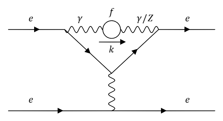
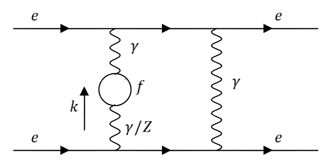
  Figure 1: Two-loop diagrams contributing to Møller scattering with a non-trivial dependence on light fermion masses.

• QCD corrections: The bulk of the higher-order QCD corrections are captured by the RG running of $\hat{s}(\mu)$, which sums up powers of large fermionic logarithms to all orders. The evaluation of $\hat{s}(0)$ in Ref. Erler:2017knj includes RG effects up to ${\cal O}(\hat{\alpha}_{\mathrm{s}}^{4})$. A separate source of QCD corrections enters through the $\rho$ parameter, which describes $m_{t}^{2}$–enhanced contributions due to custodial symmetry breaking. It contributes

  $$\Delta Q^{e}_{W}=(1-4\sin^{2}\theta_{W})\Delta\rho+\cdots\ ,$$ (19)

  where the dots indicate the remaining radiative corrections. The leading contribution is given by

  $$\Delta\rho_{(\alpha)}=\frac{3\alpha m_{t}^{2}}{16\pi\hat{s}^{2}m_{W}^{2}}~{}~{}~{}(\alpha\text{ scheme}), \Delta\rho_{(G_{\mu})}=\frac{3G_{\mu}m_{t}^{2}}{8\sqrt{2}\pi^{2}}~{}~{}~{}(G_{\mu}\text{ scheme}),$$ (20)

  and is included in the NLO correction $\Delta Q^{e,X}_{W(1,1)}$. QCD corrections from higher orders are given by Djouadi:1987gn ; Djouadi:1987di ; Kniehl:1989yc ; Avdeev:1994db ; Chetyrkin:1995ix ; Chetyrkin:2006bj ,

  $$\Delta\rho_{(X\hat{\alpha}_{\mathrm{s}}^{n})} =\Delta\rho_{(X)}\biggl{[}-\frac{4}{3}\Bigl{(}\frac{1}{2}+\frac{\pi^{2}}{6}\Bigr{)}\frac{\hat{\alpha}_{\mathrm{s}}}{\pi}-14.594\Bigl{(}\frac{\hat{\alpha}_{\mathrm{s}}}{\pi}\Bigr{)}^{2}-93.15\Bigl{(}\frac{\hat{\alpha}_{\mathrm{s}}}{\pi}\Bigr{)}^{3}+{\cal O}(\hat{\alpha}_{\mathrm{s}}^{4})\biggr{]},$$ (21)

  where $X=\alpha,G_{\mu}$. We denote these higher-order effects as

  $$X\,\Delta Q_{W,\Delta\rho}^{e,X}\equiv(1-4\hat{s}^{2})\Delta\rho_{(X\hat{\alpha}_{\mathrm{s}}^{n})}\ .$$ (22)

  With $\hat{\alpha}_{\mathrm{s}}(m_{Z})=0.1182$ one obtains the corrections listed in Table 1. The propagation of an error $\delta\hat{\alpha}_{\mathrm{s}}(m_{Z})=0.0016$ in these terms translates to $10^{-6}$ for the weak charge, which is negligible.

• Missing contributions $\Delta Q^{e,X}_{W(2,0)}$: The uncertainty in the weak charge from the missing purely bosonic NNLO corrections was estimated in Ref. Du:2021zkj to about $\pm 1.3\times 10^{-4}$.

• Higher order electroweak contributions: As can be seen from the last row of the table, the total prediction for the electron weak charge differs significantly between the $\hat{s}(m_{Z})$ scheme and the two $\hat{s}(0)$ schemes ($49.4\times 10^{-3}$ vs. $45.6\times 10^{-3}$). This difference can be attributed mainly to QCD corrections, which are missing in the former but included in the latter. The difference between the $\hat{s}(0)$–$\alpha$ and $\hat{s}(0)$–$G_{\mu}$ schemes could be regarded as an estimate of the theory error from missing higher orders (NNNLO and beyond). Its magnitude of slightly less than $10^{-4}$ is comparable to the theory error estimate for the $\Delta Q^{e,X}_{W(2,0)}$ contribution. Another way to estimate the higher-order electroweak uncertainty is to take the difference between the $\hat{s}(m_{Z})$ scheme and any of the $\hat{s}(0)$ schemes. But in order to do this one has to include the same QCD contributions in both schemes. Therefore, we first re-computed column two of Table 1 including the non-perturbative effects contained in $K_{q}$. This would include all non-perturbative effects, but would miss the resummation of the logarithms and the dependence on pQCD so that it can be compared with a re-computed column three ($\hat{s}(0)$ scheme) with pQCD turned off. The difference between these re-computed weak charges in the two schemes ($\hat{s}^{2}(0)$–$\alpha$ and $\hat{s}^{2}(m_{Z})$–$\alpha$) should then be due to electroweak effects. We found that this difference is $4.5\times 10^{-4}$, which is much smaller than the difference between columns two and three in Table 1, demonstrating that the latter is mainly due to the missing QCD effects in column two. The remaining difference may be attributed to the scheme choice. Bearing in mind that this difference is obtained in a similar way to how Ref. Czarnecki:1995fw estimated the error from the $\gamma Z$ box, we may take the interval spanned by the results in the two schemes as a conservative estimate of the higher-order perturbative error on the weak charge. Adding back the pQCD contributions, this implies that we have the error interval $[45.60,45.60+0.45]\times 10^{-3}$ or $(45.83\pm 0.23)\times 10^{-3}$, where the lower bound corresponds to the $\hat{s}^{2}(0)$–$\alpha$ result. An alternative error estimation is obtained by studying the shifts induced by the change of the weak mixing angle from $\hat{s}(m_{Z})$ to $\hat{s}(0)$ in the $\Delta Q_{W(2,1)}$ terms, leaving everything else fixed, which results in a shift of similar size ($2\times 10^{-4}$) for the weak charge.

In summary, we find for the weak charge of the electron,

$$Q^{e}_{W} =(45.83\pm 0.08_{\,\hat{s}(0)}\pm 0.06_{\Delta Q^{e,X}_{W(2,1)}(\mathrm{\,had})}\pm 0.13_{\Delta Q^{e,X}_{W(2,0)}(\mathrm{\,missing})}\pm 0.23_{\mathrm{\,scheme}})\times 10^{-3}$$

$$=\left(45.83\pm 0.28_{\mathrm{\,theory}}\right)\times 10^{-3},$$ (23)

where in the last line we added all errors in quadrature. Comparing with the experimental precision expected at MOLLER, $\delta Q_{W}^{e}=1.1\times 10^{-3}$, we see that the theoretical error is under control. In this result, the correlations between the light quark masses are properly included in the error of $\hat{s}^{2}_{0}$ computed in Ref. Erler:2017knj . For the calculation of the box and vertex diagrams, the errors on $m_{u,d}$ and $m_{s}$ are assumed to be fully anticorrelated, which is a simplifying but conservative assumption. We emphasize that the numerical difference between our result and Ref. Du:2021zkj is due to the inclusion of QCD effects, both perturbative and non-perturbative contributions parametrized by the $K_{q}$ in Ref. Erler:2017knj . To understand the impact of the scheme choice, the QCD corrections must be treated on equal footing in both schemes. This comparison has been carried out in this paper, and the difference between both schemes is taken to define the scheme error in Eq. (23). Furthermore, it is important to remark that taking half the difference between the $\hat{s}^{2}(0)$ and $\hat{s}^{2}(m_{Z})$ schemes likely overestimates the perturbative error since we expect the exact (all orders) result to be closer to the low-scale schemes. On top of that, we believe that the estimation of the electroweak perturbative error can be better understood and further reduced through a more careful resummation of dominant diagrams. Such an analysis requires the study of gauge invariant diagram subsets which is a complicated task and left for future work.

5 Finite momentum transfer effects

In the calculation of Ref. Du:2021zkj , the momentum transfer through the t- and u-channel propagators was approximated to be zero, $Q^{2}\to 0$. At the one-loop level, it was found that the shift in the transverse self-energies, $\Pi_{\rm T}^{\gamma\gamma}(-Q^{2})-\Pi_{\rm T}^{\gamma\gamma}(0)$ and $\Pi_{\rm T}^{\gamma Z}(-Q^{2})-\Pi_{\rm T}^{\gamma Z}(0)$, is very small for the kinematic parameters of the E158 and MOLLER experiments Czarnecki:1995fw . However, it is worth verifying that this also holds at two loops. This is clearly the case for diagrams where all particles in the loop have large masses, $m_{i}^{2}\gg Q^{2}$, since any momentum-dependent term scales like $Q^{2}/m_{i}^{2}$ in these contributions. But for diagrams with light fermions ($e,\mu,u,d,s$) in the loop it is less obvious that $Q^{2}\to 0$ is a good approximation.

To investigate this question, we have computed the relevant $\gamma\gamma$ and $\gamma Z$ one- and two-loop self-energies for $Q^{2}\neq 0$. The one-loop self-energies allow us to reproduce and verify the results of Ref. Czarnecki:1995fw , while the two-loop self-energies will be used to study the quality of the $Q^{2}\to 0$ approximation used in Ref. Du:2021zkj . At two-loop order, or NNLO, one also needs to include one-particle reducible diagrams with a one-loop self-energy and a one-loop vertex correction, as well as the interference of two one-loop amplitudes. We restrict ourselves to NNLO contributions with at least one closed fermion loop, since this is the order of corrections considered in Ref. Du:2021zkj . Moreover, the self-energy diagrams without fermions do not contain any particles with masses comparable to or below $Q^{2}$.

The package FeynArts 3 Hahn:2000kx has been used for generating the amplitudes for the one- and two-loop self-energies. The Lorentz and Dirac algebra has been performend with an in-house code, implemented in Mathematica. This code also performs a reduction to a set of master integrals, based on the technique of Ref. Weiglein:1993hd . The master integrals can be evaluated numerically with TVID 2 Bauberger:2019heh , which uses the one-dimensional integral representations developed in Ref. Bauberger:1994by ; Bauberger:1994hx .

As in the previous section, the hadronic self-energy contributions are described by computing quark loops and using the threshold quark masses from Ref. Erler:2017knj that have been derived from a renormalization-group analysis. As shown in Eq. (9), the impact of the $Q^{2}$-dependence of the self-energies on the asymmetry $A_{\rm LR}$ can be written as Czarnecki:1995fw

$$A_{\rm LR}=\frac{G_{\mu}Q^{2}}{\sqrt{2}\pi\alpha}\,\frac{1-y}{1+y^{4}+(1-y)^{4}}[1-4\sin^{2}\theta_{W}+F_{2}(Q^{2},y)+...],$$ (24)

where $y=Q^{2}/s$ and the dots denote all other higher-order corrections. By construction, $F_{2}(0,y)=0$.

$y$	$F_{2}^{(1,1)}\;[10^{-5}]$	$F_{2}^{(2,2)}\;[10^{-5}]$	$F_{2}^{(2,1)}\;[10^{-5}]$
0.25 (0.75)	5.01	$-$0.54	$-$0.00
0.30 (0.70)	4.11	$-$0.25	$-$0.18
0.35 (0.65)	3.39	$-$0.02	$-$0.29
0.40 (0.60)	2.86	$-$0.15	$-$0.36
0.45 (0.55)	2.55	$-$0.25	$-$0.40
0.50	2.44	$-$0.29	$-$0.41

Table 2: Numerical results for $F_{2}(Q^{2},y)$, which captures the $Q^{2}$-dependence of the photon and photon–Z self-energies. $F_{2}^{(L,n_{f})}$ denotes corrections with $L$ loops and $n_{f}$ closed fermion loops. Results are shown as a function of $y=Q^{2}/s$, for $s=0.011$ GeV² and SM input parameters in Eq. (17).

With the input parameters in Eq. (17), as well as $s=0.011$ GeV², the numerical results listed in Table 2 are obtained. The 1-loop contribution for $y=0.5$ agrees well with the analysis of Ref. Czarnecki:1995fw , which found $F_{2}(y=0.5)\approx 2\times 10^{-5}$. For all experimentally relevant values of $y$, the NLO contributions to $F_{2}$ stay well below $10^{-4}$ and thus are irrelevant for practical purposes. The NNLO contributions can be divided into terms with two and one closed fermion loop. Both of these, as well as the sum of the NNLO effects, are about one order of magnitude smaller than the NLO contributions. This confirms that the $Q^{2}\to 0$ approximation used in Ref. Du:2021zkj is accurate and robust at NLO and NNLO.

6 Conclusions

The left-right polarization asymmetry in Møller scattering is a sensitive probe of parity violation in the SM and from new physics. Recently, the SM electroweak two-loop corrections from contributions with closed fermion loops to this observable were computed in Ref. Du:2021zkj . For phenomenlogical applications, this result needs to be combined with resummed QCD and hadronic effects, which can be incorporated through the renormalization group analysis of the $\overline{\text{MS}}$ weak mixing angle $\hat{s}(\mu)$ at low scales $\mu\approx 0$ Erler:2004in ; Erler:2017knj . Two new schemes are introduced, labeled $\hat{s}(0)$–$\alpha$ and $\hat{s}(0)$–$G_{\mu}$, respectively. Both use the low-energy $\overline{\text{MS}}$ weak mixing angle as input, but the former scheme uses $\alpha$ for the power counting of the electroweak perturbative expansion, whereas the latter uses $G_{\mu}$.

In addition to the perturbative and non-perturbative QCD effects from the running of $\hat{s}(\mu)$, we also include perturbative QCD corrections to the $\rho$ parameter. Finally, we carry out a careful analysis of the dependence of the scattering rate on the momentum transfer squared $Q^{2}$, which we find to be numerically negligible. The SM prediction for the left-right asymmetry, including higher-order effects, can be expressed in terms of the weak charge $Q_{W}^{e}$ of the electron. In the $\hat{s}(0)$–$\alpha$ scheme we obtain $Q_{W}^{e}=(45.83\pm 0.28)\times 10^{-3}$, where the dominant error of $\pm 0.23\times 10^{-3}$ stems from the purely electroweak difference between the $\hat{s}(m_{Z})$-$\alpha$ and $\hat{s}(0)$-$\alpha$ schemes. The result is consistent with the one-loop calculation of Ref. Czarnecki:1995fw and implies a reduction of the uncertainty by almost an order of magnitude. Additional relevant sources of uncertainty stem from the currently unknown bosonic two-loop corrections (estimated as $\delta Q^{e}_{W}=\pm 0.13\times 10^{-3}$ Du:2021zkj ) and from the running of $\hat{s}(\mu)$ including non-perturbative effects (estimated to amount to $\delta Q^{e}_{W}=\pm 0.08\times 10^{-3}$ Erler:2017knj ). When compared to the expected precision $\delta Q_{W}^{e}=1.1\times 10^{-3}$ of the planned MOLLER experiment Benesch:2014bas , the overall uncertainty of the SM prediction turns out to be insignificant. Furthermore, this theoretical error is rather conservative, since the low-energy scale of the process suggests that the $\hat{s}(0)$ scheme is the more adequate one to use in the tree-level expression, so that considering half the scheme difference may overestimate the uncertainty. Future work on enhanced three-loop effects and the purely bosonic two-loop corrections can be expected to reduce the theory error further.

References

- (1) MOLLER collaboration, The MOLLER Experiment: An Ultra-Precise Measurement of the Weak Mixing Angle Using Møller Scattering, 1411.4088.
- (2) SLAC E158 collaboration, Precision measurement of the weak mixing angle in Moller scattering, Phys. Rev. Lett. 95 (2005) 081601 [hep-ex/0504049].
- (3) E. Derman and W.J. Marciano, Parity Violating Asymmetries in Polarized Electron Scattering, Annals Phys. 121 (1979) 147.
- (4) A. Czarnecki and W.J. Marciano, Electroweak radiative corrections to polarized Moller scattering asymmetries, Phys. Rev. D53 (1996) 1066 [hep-ph/9507420].
- (5) Y. Du, A. Freitas, H.H. Patel and M.J. Ramsey-Musolf, Parity-Violating Møller Scattering at Next-to-Next-to-Leading Order: Closed Fermion Loops, Phys. Rev. Lett. 126 (2021) 131801 [1912.08220].
- (6) W.J. Marciano, Spin and precision electroweak physics, in Spin structure in high-energy processes: Proceedings, 21st SLAC Summer Institute on Particle Physics, 26 Jul - 6 Aug 1993, Stanford, CA, L. DePorcel and C. Dunwoodie, eds., 1995, http://www.slac.stanford.edu/spires/find/books/www?cl=QCD161:S76:1993.
- (7) A. Czarnecki and W.J. Marciano, Parity violating asymmetries at future lepton colliders, Int. J. Mod. Phys. A13 (1998) 2235 [hep-ph/9801394].
- (8) J. Erler and M.J. Ramsey-Musolf, The Weak mixing angle at low energies, Phys. Rev. D72 (2005) 073003 [hep-ph/0409169].
- (9) J. Erler and R. Ferro-Hernández, Weak Mixing Angle in the Thomson Limit, JHEP 03 (2018) 196 [1712.09146].
- (10) M. Davier, A. Hoecker, B. Malaescu and Z. Zhang, A new evaluation of the hadronic vacuum polarisation contributions to the muon anomalous magnetic moment and to , Eur. Phys. J. C 80 (2020) 241 [1908.00921].
- (11) A. Keshavarzi, D. Nomura and T. Teubner, of charged leptons, , and the hyperfine splitting of muonium, Phys. Rev. D 101 (2020) 014029 [1911.00367].
- (12) F. Jegerlehner, (s) for precision physics at the FCC-ee/ILC, in Theory for the FCC-ee: Report on the 11th FCC-ee Workshop Theory and Experiments, A. Blondel, J. Gluza, S. Jadach, P. Janot and T. Riemann, eds., vol. 3/2020 of CERN Yellow Reports: Monographs, pp. 9–37, 2020, DOI.
- (13) RBC/UKQCD collaboration, Lattice calculation of the leading strange quark-connected contribution to the muon , JHEP 04 (2016) 063 [1602.01767].
- (14) A. Freitas, W. Hollik, W. Walter and G. Weiglein, Complete fermionic two loop results for the M(W) - M(Z) interdependence, Phys. Lett. B495 (2000) 338 [hep-ph/0007091].
- (15) A. Freitas, W. Hollik, W. Walter and G. Weiglein, Electroweak two loop corrections to the mass correlation in the standard model, Nucl. Phys. B632 (2002) 189 [hep-ph/0202131].
- (16) M. Awramik and M. Czakon, Complete two loop electroweak contributions to the muon lifetime in the standard model, Phys. Lett. B568 (2003) 48 [hep-ph/0305248].
- (17) C. Sturm, Leptonic contributions to the effective electromagnetic coupling at four-loop order in QED, Nucl. Phys. B874 (2013) 698 [1305.0581].
- (18) M. Cè, A. Gérardin, G. von Hippel, H.B. Meyer, K. Miura, K. Ottnad et al., The hadronic running of the electromagnetic coupling and the electroweak mixing angle from lattice QCD, 2203.08676.
- (19) A. Blondel, J. Gluza, S. Jadach, P. Janot and T. Riemann, eds., Theory for the FCC-ee: Report on the 11th FCC-ee Workshop Theory and Experiments, vol. 3/2020 of CERN Yellow Reports: Monographs, (Geneva), CERN, 5, 2019. 10.23731/CYRM-2020-003.
- (20) M. Fael and M. Passera, Muon-Electron Scattering at Next-To-Next-To-Leading Order: The Hadronic Corrections, Phys. Rev. Lett. 122 (2019) 192001 [1901.03106].
- (21) M. Fael, Hadronic corrections to - scattering at NNLO with space-like data, JHEP 02 (2019) 027 [1808.08233].
- (22) A. Djouadi and C. Verzegnassi, Virtual Very Heavy Top Effects in LEP / SLC Precision Measurements, Phys. Lett. B 195 (1987) 265.
- (23) A. Djouadi, O(alpha alpha-s) Vacuum Polarization Functions of the Standard Model Gauge Bosons, Nuovo Cim. A 100 (1988) 357.
- (24) B.A. Kniehl, Two Loop Corrections to the Vacuum Polarizations in Perturbative QCD, Nucl. Phys. B 347 (1990) 86.
- (25) L. Avdeev, J. Fleischer, S. Mikhailov and O. Tarasov, correction to the electroweak parameter, Phys. Lett. B 336 (1994) 560 [hep-ph/9406363].
- (26) K.G. Chetyrkin, J.H. Kuhn and M. Steinhauser, Corrections of order to the parameter, Phys. Lett. B 351 (1995) 331 [hep-ph/9502291].
- (27) K.G. Chetyrkin, M. Faisst, J.H. Kuhn, P. Maierhofer and C. Sturm, Four-Loop QCD Corrections to the Rho Parameter, Phys. Rev. Lett. 97 (2006) 102003 [hep-ph/0605201].
- (28) T. Hahn, Generating Feynman diagrams and amplitudes with FeynArts 3, Comput. Phys. Commun. 140 (2001) 418 [hep-ph/0012260].
- (29) G. Weiglein, R. Scharf and M. Bohm, Reduction of general two loop selfenergies to standard scalar integrals, Nucl. Phys. B416 (1994) 606 [hep-ph/9310358].
- (30) S. Bauberger, A. Freitas and D. Wiegand, TVID 2: Evaluation of planar-type three-loop self-energy integrals with arbitrary masses, JHEP 01 (2020) 024 [1908.09887].
- (31) S. Bauberger, F.A. Berends, M. Bohm and M. Buza, Analytical and numerical methods for massive two loop selfenergy diagrams, Nucl. Phys. B434 (1995) 383 [hep-ph/9409388].
- (32) S. Bauberger and M. Bohm, Simple one-dimensional integral representations for two loop selfenergies: The Master diagram, Nucl. Phys. B 445 (1995) 25 [hep-ph/9501201].