Looking for the exotic $X_{0}(2866)$ and its $J^{P}=1^{+}$ partner in the $\bar{B}^{0}\to D^{(*)+}K^{-}K^{(*)0}$ reactions

Abstract

We propose two reactions, $\bar{B}^{0}\to K^{0}D^{+}K^{-}$ and $\bar{B}^{0}\to K^{*0}D^{*+}K^{-}$, already measured at Belle, to look into the $J^{P}=0^{+}$, $X_{0}(2866)$ state and a $1^{+}$ partner of molecular $D^{*}\bar{K}^{*}$ nature, by looking at the $D^{+}K^{-}$ and $D^{*+}K^{-}$ invariant mass distributions, respectively. Very clear peaks over the background are predicted and the branching ratios for the production of these states are evaluated to facilitate the task of determining the needed statistics for their observation. The fact that the $K^{*0}K^{-}$ mass distribution from accumulation of events of different reactions is already available, indicates that one is not far away from having the needed statistics to see peaks in the $D^{(*)+}K^{-}$ mass distributions, so far not yet analyzed.

I Introduction

In the paper belle the Belle collaboration reported on the $\bar{B}^{0}\to D^{(*)+}K^{-}K^{(*)0}$ decays, giving a list of eight reactions for which the branching ratios were provided. In some of the reactions: a) $\bar{B}^{0}\to D^{+}K^{-}K^{*0}$, b) $\bar{B}^{0}\to D^{*+}K^{-}K^{*0}$, c) $\bar{B}^{0}\to D^{+}K^{-}K^{0}$, d) $\bar{B}^{0}\to D^{*+}K^{-}K^{0}$, one finds pairs, $D^{+}K^{-}$ in $a)$ and $c)$, $D^{*+}K^{-}$ in $b)$ and $d)$, which contain open charm and strangeness with $c$ and $s$ quarks. Should these pairs result from the decay of a physical state, it would be genuinely exotic since it cannot come from a $q\bar{q}$ conventional meson. The chosen pairs could correspond to states with isospin $I=0$, while the other four cases of belle would correspond to $D^{(*)+}\bar{K}$ states with isospin $I=1$. The limited statistics prevented to get $D^{(*)+}K^{-}$ mass distributions, while the accumulation of $K^{-}K^{*0}$ events from four reactions allowed to get a $K^{-}K^{*0}$ mass distribution that evidenced the $B\to D^{(*)+}a_{1}(1260)$ decay with $a_{1}(1260)\to K^{-}K^{*0}$. Yet, the abundant literature on tetraquark states from the very beginning of the quark model rm1 ; rm2 ; rm3 ; rm4 ; rm5 ; rm8 ; rm9 ; rm7 ; rm6 ; rm11 ; rm10 up to now (see Refs. hxchen ; ahmed ; pilloni ; rosner ; xliu ; nora for reviews on more recent works), would have made advisable to look at the $D^{(*)+}\bar{K}$ mass distributions in search of possible peaks corresponding to exotic states.

In between, the answer to this question was provided by the LHCb collaboration lhcb1 ; lhcb2 with the finding of the $X_{0}(2866)$ and $X_{1}(2900)$ states in the $B^{+}\to D^{+}D^{-}K^{+}$ decay by looking at the $D^{-}K^{+}$ invariant mass distribution. In the charge conjugate reaction $B^{-}\to D^{+}D^{-}K^{-}$ one would find the peaks in the $D^{+}K^{-}$ invariant mass distribution. Interestingly, the existence of a $I=0,J^{P}=0^{+}$ molecular state of $D^{*}\bar{K}^{*}$ nature, decaying to $D\bar{K}$, had been predicted in tania , with a mass of $2848\textrm{ MeV}$ and a width between $23-59\textrm{ MeV}$, very close to the data of the $X_{0}(2866)$ with mass $2866\pm 7\textrm{ MeV}$ and width $57.2\pm 12.9\textrm{ MeV}$. An update of that work to the light of the LHCb results is presented in raquelx .

The findings of Refs. lhcb1 ; lhcb2 prompted many works offering an explanation for the $X_{0}(2866)$ as a tetraquark state d5 ; d6 ; d7 ; d8 or a molecular $D^{*}\bar{K}^{*}$ state d14 ; d15 ; d16 ; d17 ; d18 ; d19 . The sum rules studies d9 ; d10 ; d11 ; d12 ; d13 have also contributed its share to the discussion, some of them proposing a molecular structure d11 ; d12 ; d13 . Other studies suggest a structure coming from a triangle singularity d21 or cusps and analytical properties of triangle diagrams d22 ; d23 . A triangle mechanism is also suggested in qifang , and in d20 a detailed quark model calculation is shown to disfavor the compact tetraquark picture.

In Ref. tania , apart from the $J^{P}=0^{+}$ state, two other states with $J^{P}=1^{+},2^{+}$ also in $I=0$ were found. In the update of raquelx , where the free parameters of the model were adjusted to experiment lhcb1 for the $X_{0}(2866)$, the masses, widths and couplings to the $D^{*}\bar{K}^{*}$ channel were evaluated, which are shown in Table 1.

Table 1: Properties of the $D^{*}\bar{K}^{*}$ states from Ref. raquelx accounting for $D\bar{K}$ and $D^{*}\bar{K}$ decays.

$I[J^{P}]$	$M~{}[\mathrm{MeV}]$	$\Gamma~{}[\mathrm{MeV}]$	Coupled channels	$g_{R,D^{*}\bar{K}^{*}}$ $[\mathrm{MeV}]$	state
$0[2^{+}]$	$2775$	$38$	$D^{*}\bar{K}^{*}$	$16536$	?
$0[1^{+}]$	$2861$	$20$	$D^{*}\bar{K}^{*}$	$12056$	?
$0[0^{+}]$	$2866$	$57$	$D^{*}\bar{K}^{*}$	$11276$	$X_{0}(2866)$

For reasons of parity and angular momentum conservations, the $0^{+}$ state only decays to $D\bar{K}$ while the $1^{+}$ state decays to $D^{*}\bar{K}$.

The purpose of the present work is to investigate whether by looking at the $\bar{B}^{0}\to D^{(*)+}K^{-}K^{(*)0}$ reactions one can observe clear peaks in the $D^{(*)+}K^{-}$ spectrum. The reaction is similar to the $B^{-}\to D^{+}D^{-}K^{-}$ one studied in lhcb1 ; lhcb2 . The $K^{(*)0}$ in the Belle reactions would play the role of the $D^{-}$ in the LHCb one. The study is stimulated by the success found in newpaper , fairly reproducing the $D\bar{K}$ peak versus the background of lhcb1 in the study of the $B^{-}\to D^{+}D^{-}K^{-}$ reaction. This success was used in newpaper to suggest the $\bar{B}^{0}\to D^{*+}D^{*0}K^{-}$ decay in order to investigate the $1^{+}$ state of Table 1 by looking at the $D^{*+}K^{-}$ mass distribution. It was found that the $1^{+}$ state generated a peak in the distribution with a strength about $7$ times bigger than the background at the peak of the $1^{+}$ contribution. Based on these findings we propose here to study the $\bar{B}^{0}\to D^{*+}K^{-}K^{*0}$ and $\bar{B}^{0}\to D^{+}K^{-}K^{0}$ reactions. The reason to choose these two reactions between the eight reactions of Belle belle is that, both in the signal for the exotic states as in the background, the amplitudes can proceed in $s$-wave, assumed dominant as usual, and one can correlate the background and the signal for the production of the $0^{+}$ and $1^{+}$ states.

II FORMALISM and results

II.1 Production of the $1^{+}$ state in $\bar{B}^{0}\to D^{*+}K^{*-}K^{*0}\to D^{*+}K^{-}K^{*0}$

The $D^{*}\bar{K}^{*}$ $1^{+}$ state can only decay in $D^{*}\bar{K}$. Thus, we choose the $\bar{B}^{0}\to D^{*+}K^{-}K^{*0}$ reaction and look at $D^{*+}K^{-}$ mass distribution. The signal, however, will come from the $\bar{B}^{0}\to D^{*+}K^{*-}K^{*0}$ reaction, after the final state interaction of $D^{*+}K^{*-}$ to give the $1^{+}$ state ($R_{1}$) and posterior decay into $D^{*+}K^{-}$. The primary step proceeds via external emission as depicted in Fig. 1.

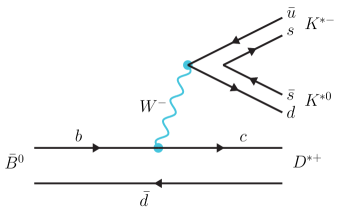
Figure 1: Diagrammatic decay of $\bar{B}^{0}\to D^{*+}K^{*-}K^{*0}$ at the quark level.

The $\bar{u}d$ component after the $W^{-}$ vertex is hadronized with an $s\bar{s}$ component to give rise to $K^{*-}K^{*0}$ and the $c\bar{d}$ gives the $D^{*+}$. One has three vectors and one can write the $s$-wave component of the transition matrix matching the angular momentum of the $\bar{B}^{0}$ as:

$$\tilde{t}={\cal{C}}\,{\bm{\epsilon}^{(1)}}\cdot({\bm{\epsilon}^{(2)}}\times{\bm{\epsilon}^{(3)}})={\cal{C}}\,\epsilon_{ijk}\epsilon^{(1)}_{i}\epsilon^{(2)}_{j}\epsilon^{(3)}_{k}$$ (1)

where the indices $1,2,3$ apply to the $K^{*0}$, $D^{*0}$ and $K^{*-}$, respectively. We observe how the spins of the particles $2$ and $3$ combine to $J=1$. The next step is to consider the $D^{*+}K^{*-}$ interaction. With our phase convention $(D^{*+},-D^{*0})$, $(\bar{D}^{*0},D^{*-})$, $(K^{*+},K^{*0})$, $(\bar{K}^{*0},-K^{*-})$, the $I=0$ $D^{*}\bar{K}^{*}$ state is written as

$$|D^{*}\bar{K}^{*};I=0\rangle=-\frac{1}{\sqrt{2}}(D^{*+}K^{*-}+D^{*0}\bar{K}^{*0})\,.$$ (2)

The final state interaction of $D^{*+}K^{*-}$ to produce the $R_{1}$ state is taken into account as shown diagrammatically in Fig. 2.

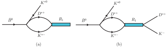
Figure 2: (a) Rescattering of $D^{*+}K^{*-}$ to give the resonance $R_{1}$; (b) Further decay of $R_{1}$ into $D^{*+}K^{-}$.

We also need the vertex $R_{1}D^{*}\bar{K}^{*}$ which incorporates the spin projection generator $D^{i}$

$$\tilde{g}_{i}=g_{i}V^{(i)}$$ (3)

with $V^{(i)}$ given by liangmolina

$$V^{(0)} = \frac{1}{3}\epsilon^{(2)}_{l}\epsilon^{(3)}_{l}\delta_{ij}$$

$$V^{(1)} = \frac{1}{2}\big{(}\epsilon^{(2)}_{i}\epsilon^{(3)}_{j}-\epsilon^{(2)}_{j}\epsilon^{(3)}_{i}\big{)}$$

$$V^{(2)} = \frac{1}{2}\big{(}\epsilon^{(2)}_{i}\epsilon^{(3)}_{j}+\epsilon^{(2)}_{j}\epsilon^{(3)}_{i}\big{)}-\frac{1}{3}\epsilon^{(2)}_{l}\epsilon^{(3)}_{l}\delta_{ij}$$ (4)

Considering the $\tilde{t}$ matrix of Eq. (1) and Eq. (3) for $V^{(1)}$, $V^{(1)}=\frac{1}{2}\big{(}\epsilon^{(2)}_{i^{\prime}}\epsilon^{(3)}_{j^{\prime}}-\epsilon^{(2)}_{j^{\prime}}\epsilon^{(3)}_{i^{\prime}}\big{)}$, and that in the loop function we sum over the spin polarization $\sum_{pol}\epsilon^{(r)}_{i}\epsilon^{(r)}_{j}=\delta_{ij}~{}(r=2,3)$, we obtain

$$t={\cal{C}}\,\epsilon^{(1)}\epsilon_{ii^{\prime}j^{\prime}}G_{D^{*}\bar{K}^{*}}(M_{\rm inv}(D^{*}\bar{K}^{*}))\frac{-1}{\sqrt{2}}g_{R,D^{*}\bar{K}^{*}}$$

where $g_{R_{1},D^{*}\bar{K}^{*}}$ is the coupling of the resonance $R_{1}$ to the $(I=0)$ $D^{*}\bar{K}^{*}$ state and $G_{D^{*}\bar{K}^{*}}$ is the loop function of the $D^{*},\bar{K}^{*}$ integrating the propagators of the two particles. We use dimensional regularization for this loop with $\alpha=-1.474$ for a chosen $\mu=1500\textrm{ MeV}$ as was needed in raquelx to obtain the right mass of the $X_{0}(2866)$ state.

The sum over the final vector polarization in $\sum|t|^{2}$ is implemented by summing $\sum|t|^{2}$ over the indices $i^{\prime},j^{\prime}$ for the implicit $VV$ components of $R_{1}$ and over the index $i$ to sum over the $K^{*0}$ polarization. We find

$$\sum_{pol}|t|^{2} = 3\,{\cal{C}}^{2}\,|g_{R_{1},D^{*}\bar{K}^{*}}|^{2}\,|G_{D^{*}\bar{K}^{*}}(M_{\rm inv}(D^{*}\bar{K}^{*}))|^{2}$$

The next step is to consider the decay of $R_{1}$ into $D^{*+}K^{-}$, as depicted in Fig. 2 (b). This leads to a $t^{\prime}$ matrix containing the coupling of $R_{1}$ to $D^{*+}K^{-}$. This is accomplished by an effective coupling $g_{R_{1},D^{*}\bar{K}}$ to the $D^{*}\bar{K}^{*},I=0$ state, such that the coupling to $D^{*+}K^{-}$ is $\frac{-1}{\sqrt{2}}g_{R_{1},D^{*}\bar{K}}$. To get the $g_{R_{1},D^{*}\bar{K}}$ coupling we use the $R_{1}$ decay width via

$$\Gamma_{R_{1}}=\frac{1}{8\pi}\frac{1}{M^{2}_{R_{1}}}|g_{R_{1},D^{*}\bar{K}}|^{2}q_{\bar{K}}\,;\qquad q_{\bar{K}}=\frac{\lambda^{1/2}(M^{2}_{R_{1}},m^{2}_{D^{*}},m^{2}_{\bar{K}})}{2M_{R_{1}}}\ ,$$ (5)

taking the value of $\Gamma_{R_{1}}$ from Table 1. Hence

$$\sum_{pol}|t^{\prime}|^{2} = \frac{6}{4}{\cal{C}}^{2}|g_{R_{1},D^{*}\bar{K}^{*}}|^{2}|G_{D^{*}\bar{K}^{*}}(M_{\rm inv})|^{2}$$ (6)

$$\times |g_{R_{1},D^{*}\bar{K}}|^{2}|\frac{1}{M^{2}_{\rm inv}(R_{1})-M^{2}_{R_{1}}+iM_{R_{1}}\Gamma_{R_{1}}}|^{2}$$

The invariant mass distribution is then given by

$$\frac{d\Gamma}{dM_{\rm inv}(D^{*+}K^{-})}=\frac{1}{(2\pi)^{3}}\frac{1}{4M^{2}_{\bar{B}^{0}}}p_{\bar{K}^{*0}}\tilde{p}_{K^{-}}\sum|t^{\prime}|^{2}$$ (7)

where

$$p_{\bar{K}^{*0}}=\frac{\lambda^{1/2}(M^{2}_{\bar{B}^{0}},m^{2}_{\bar{K}^{*0}},M^{2}_{\rm inv}(D^{*+}K^{-})}{2M_{\bar{B}^{0}}}\,,\quad\tilde{p}_{K^{-}}=\frac{\lambda^{1/2}(M^{2}_{\rm inv}(D^{*+}K^{-}),m^{2}_{D^{*}},m^{2}_{\bar{K}})}{2M_{\rm inv}(D^{*+}K^{-})}$$ (8)

We would like to compare this mass distribution with the one of the background for the same reaction, $\bar{B}^{0}\to K^{*0}D^{*+}K^{-}$. The process proceeds with the same topology as in Fig. 1, changing $K^{*-}$ by $K^{-}$. As shown in vectorpseudo the difference between pseudoscalar and vector production can be taken into account by means of Racah coefficients of the same order of magnitude, so approximately we can put for the $\bar{B}^{0}\to K^{*0}D^{*+}K^{-}$ background

$$t={\cal{C}}\,{\bm{\epsilon}(K^{*})}\,{\bm{\epsilon}(D^{*})}$$

with the same constant ${\cal{C}}$ as in Eq. (1), such that now the background distribution is given by

$$\frac{d\Gamma_{\rm bac}}{dM_{\rm inv}(D^{*+}K^{-})}=\frac{1}{(2\pi)^{3}}\frac{1}{4M^{2}_{\bar{B}^{0}}}p_{K^{*0}}\tilde{p}_{\bar{K}}\,3\,{\cal{C}}^{2}$$ (9)

The assumption of taking the same constant ${\cal{C}}$ is supported by the results of newpaper , reproducing fairly well the signal versus the background of the LHCb experiment lhcb1 .

The results can be seen in Fig. 3. We can see a peak clearly sticking out of the background, as was also found in newpaper with a different reaction. It is clear that even if there were uncertainties of a factor of two or three, the signal should be clearly seen.

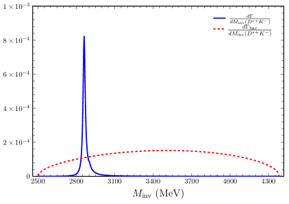
Figure 3: $\frac{d\Gamma}{dM_{\rm inv}}$ for $R_{1}$ production and $\frac{d\Gamma_{\rm bac}}{dM_{\rm inv}}$ for background in the $\bar{B}^{0}\to K^{*0}D^{*+}K^{-}$ reaction in global arbitrary units. $M_{\rm inv}$ is the $D^{*+}K^{-}$ invariant mass.

II.2 Production of the $0^{+}$ state in $\bar{B}^{0}\to K^{0}D^{*+}K^{*-}\to K^{0}D^{+}K^{-}$

Proceeding like in the former subsection, we would now compare the signal for the $0^{+}$ state from the $\bar{B}^{0}\to K^{0}D^{*+}K^{*-}$ with $D^{*+}K^{*-}$ interaction leading to the $0^{+}$ state ($R_{0}$) and its decay into $D^{+}K^{-}$, and the background from the $\bar{B}^{0}\to K^{0}D^{+}K^{-}$ reaction. We can proceed as before and for the $\bar{B}^{0}\to K^{0}D^{*+}K^{*-}$ we assume a transition matrix

$$t={\cal{C^{\prime}}}\,{\bm{\epsilon}(D^{*})}\,{\bm{\epsilon}(K^{*})}$$

and similarly for the $\bar{B}^{0}\to K^{0}D^{+}K^{-}$

$$t={\cal{C^{\prime}}}$$

with the same ${\cal{C^{\prime}}}$ as we have done before. We shall come back to this assumption. Following the same steps as before we obtain:

$$\frac{d\Gamma^{\prime}}{dM_{\rm inv}(D^{+}K^{-})}=\frac{1}{(2\pi)^{3}}\frac{1}{4M^{2}_{\bar{B}^{0}}}p_{K^{0}}\tilde{p}_{K^{-}}\sum|t^{\prime}|^{2}$$ (10)

where

$$\sum|t^{\prime}|^{2} = \frac{3}{4}{\cal{C^{\prime}}}^{2}|G_{D^{*}\bar{K}^{*}}(M_{\rm inv}(D^{+}K^{-}))|^{2}\,|g_{R_{0},D^{*}\bar{K}^{*}}|^{2}$$ (11)

$$\times |\frac{1}{M^{2}_{\rm inv}(D^{+}K^{-})-M^{2}_{R_{0}}+iM_{R_{0}}\Gamma_{R_{0}}}|^{2}\,|g_{R_{0},D\bar{K}}|^{2}$$

with

$$p_{K^{0}}=\frac{\lambda^{1/2}(M^{2}_{\bar{B}^{0}},m^{2}_{K^{0}},M^{2}_{\rm inv}(D^{+}K^{-})}{2M_{\bar{B}^{0}}}\,,\quad\tilde{p}_{K^{-}}=\frac{\lambda^{1/2}(M^{2}_{\rm inv}(D^{+}K^{-}),m^{2}_{D^{+}},m^{2}_{K^{-}})}{2M_{\rm inv}(D^{+}K^{-})}$$ (12)

with $g_{R_{0},D^{*}\bar{K}^{*}}$ given in Table 1, and the effective $|g_{R_{0},D\bar{K}}|^{2}$ coupling obtained from

$$\Gamma_{R_{0}}=\frac{1}{8\pi}\frac{1}{M^{2}_{R_{0}}}|g_{R_{0},D\bar{K}}|^{2}q_{\bar{K}}\,;\qquad q_{\bar{K}}=\frac{\lambda^{1/2}(M^{2}_{R_{0}},m^{2}_{D^{+}},m^{2}_{\bar{K}})}{2M_{R_{0}}}$$ (13)

For the background we find

$$\frac{d\Gamma^{\prime}_{\rm bac}}{dM_{\rm inv}(D^{+}K^{-})}=\frac{1}{(2\pi)^{3}}\frac{1}{4M^{2}_{\bar{B}^{0}}}p_{K^{0}}\tilde{p}_{K^{-}}\,{\cal{C^{\prime}}}^{2}$$ (14)

The results for these two distributions are shown in Fig. 4. We also see a signal that sticks out of the background clearly, as was shown in newpaper for the $B^{-}\to D^{+}D^{-}K^{-}$ reaction in the production of the $X_{0}(2866)$.

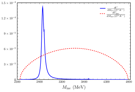
Figure 4: $\frac{d\Gamma^{\prime}}{dM_{\rm inv}}$ for $R_{0}$ production and $\frac{d\Gamma^{\prime}_{\rm bac}}{dM_{\rm inv}}$ for background in the $\bar{B}^{0}\to K^{+}D^{+}K^{-}$ reaction in global arbitrary units. $M_{\rm inv}$ is the $D^{+}K^{-}$ invariant mass.

As this point we would like to make some discussion. The $\bar{B}^{0}\to K^{0}D^{*+}K^{*-}$ can proceed with the topology of Fig. 1 changing $K^{*0}$ by $K^{0}$ where the $K^{0}$ and $K^{*-}$ are produced by hadronization of the $\bar{u}d$ component. Yet, the production of $K^{0}K^{-}$ from the same vertex is suppressed, as discussed in notwops . Indeed, the vertex $WPP$ is given by $W_{\mu}\langle[P,\partial_{\mu}P]\rangle$ in chiral theory chiral1 ; chiral2 , the $s$-wave going as the difference in the energies of the two pseudoscalars for the $WPP$ vertex, which vanishes in the $W$ rest frame if the particles have the same mass. The argument does not hold if one produces a vector and a pseudoscalar, as it was the case for the signal of the $0^{+}$ state. The argument given above is corroborated by the branching ratio of the $\bar{B}^{0}\to D^{+}K^{-}K^{0}$, which is about one order of magnitude smaller than the one of $\bar{B}^{0}\to D^{*+}K^{-}K^{*0}$ (see table 2 of Ref. belle ). Certainly we could now have contributions from higher partial waves, but the argumentation given above, with the support of the small $\bar{B}^{0}\to D^{+}K^{-}K^{0}$ branching ratio, would tell us that we can expect in practice a peak showing even stronger with respect to the background than what is shown in Fig. 4.

In the LHCb case lhcb1 a different reaction was used, the $B^{+}\to D^{+}D^{-}K^{+}$, or analogously $B^{-}\to D^{-}D^{+}K^{-}$. Even if the reaction seems the same except for small changes as the $\bar{B}^{0}\to K^{0}D^{+}K^{-}$, replacing the $D^{-}$ by $K^{0}$, the reactions are topologically different since the LHCb one, as well as the associated $B^{-}\to D^{-}D^{*+}K^{*-}$ reaction, proceed via internal emission and the argument discussed above is peculiar of the $W^{\mu}\langle[P,\partial_{\mu}P]\rangle$ vertex of external emission. In the LHCb reaction the formalism used here for the signal and background gave rise to a distribution in fair agreement with experiment. There is no analog reaction to the $B^{-}\to D^{-}D^{+}K^{-}$ that proceeds with internal emission of the type $B\to DK\bar{K}$. The reaction that we have chosen to observe the $0^{+}$, $X_{0}(2866)$ state, $\bar{B}^{0}\to K^{0}D^{+}K^{-}$, stands as a good one, where the signal over background is expected to be even bigger than shown in Fig. 4.

III Conclusions

We have chosen two reactions, already performed by the Belle collaboration belle , to observe the $0^{+},1^{+}$ states obtained from the $D^{*}\bar{K}^{*}$ interaction, where the $0^{+}$ state is associated to the $X_{0}(2866)$ state. From the eight reactions of the type $\bar{B}\to D^{(*)}K^{-}K^{*0}$ of Ref. belle we have selected two, the $\bar{B}^{0}\to K^{*0}D^{*+}K^{-}$ and $\bar{B}^{0}\to K^{0}D^{+}K^{-}$, in order to observe the $1^{+}$ and $0^{+}$ states respectively. In the first case the signal of the $1^{+}$ state stems from the original $\bar{B}^{0}\to K^{*0}D^{*+}K^{*-}$ reaction, followed by $D^{*+}K^{*-}$ interaction to give the $R_{1}$ resonance, which decays posteriorly to $D^{*+}K^{-}$. In the second case, the signal for the $0^{+}$ state comes from the $\bar{B}^{0}\to K^{0}D^{*+}K^{*-}$ with posterior $D^{*+}K^{-}$ interaction to produce the $0^{+}$ state, which decays lately into $D^{+}K^{-}$. We could relate the mass distributions of the signal and the background, finding very clear peaks for the $1^{+}$ and $0^{+}$ states. However, we have argued that in the case of the $0^{+}$ state we expect the signal to be even more pronounced with respect to background than what is calculated here because of the suppressed $\bar{B}^{0}\to D^{+}K^{-}K^{0}$ decay versus $\bar{B}^{0}\to D^{*+}K^{-}K^{*0}$ decay at the tree level.

These reactions, already measured at Belle belle , would need somewhat more statistics to show the $D^{(*)+}K^{-}$ peaks clearly. To facilitate the task of determining the needed statistics, we have performed the integrated widths and we find

$$\Gamma(\bar{B}^{0}\to K^{*0}1^{+};1^{+}\to D^{*+}K^{-})/\Gamma(\bar{B}^{0}\to K^{*0}D^{*+}K^{-})=1.25\times 10^{-1}\,,$$

$$\Gamma(\bar{B}^{0}\to K^{0}0^{+};0^{+}\to D^{+}K^{-})/\Gamma(\bar{B}^{0}\to K^{0}D^{+}K^{-})=1.24\times 10^{-1}\,.$$

Together with the branching ratios of the backgrounds of $12.9\times 10^{-4}$, $1.6\times 10^{-4}$ respectively for the former two reactions belle , the branching ratios for the exotic states produced stand well within the experimental range presently accessible in $B$ decays pdg . Thus, we can only encourage the performance of the experiment that should corroborate the existence of the $X_{0}(2866)$ related to the existence of the associated $1^{+}$ state. Since actually the $K\bar{K}^{*0}$ invariant mass distribution was already shown in Ref. belle from accumulation of events in different reactions, this means that one is not far from having enough statistics to see the unmeasured $D^{(*)+}K^{-}$ peaks from the individual reactions. The other associated state $2^{+}$ is not easy to see with this kind of reactions and will have to wait its turn with different ones.

References

- (1) A. Drutskoy, et al. (Belle Collaboration), Phys. Lett. B 542, 171 (2002)
- (2) M. Gell-Mann, Phys. Lett. 8, 214 (1964)
- (3) G. Zweig, An SU(3) model for strong interaction symmetry and its breaking, Version 1, CERN-TH-401, 1964
- (4) R. L. Jaffe, Phys. Rev. D 15, 267 (1977)
- (5) R. L. Jaffe, Phys. Rev. D 15, 281 (1977)
- (6) H. M. Chan, H. Hogaasen, Phys. Lett. B 72, 121 (1977)
- (7) H. Hogaasen, P. Sorba, Nucl. Phys. B 145, 119 (1978)
- (8) D. Strottman, Phys. Rev. D 20, 748 (1979)
- (9) K. T. Chao, Nucl. Phys. B 169, 281 (1980)
- (10) K. T. Chao, Nucl. Phys. B 183, 435 (1981)
- (11) C. Gignoux, B. Silvestre-Brac, J. M. Richard, Phys. Lett. B 193, 323 (1987)
- (12) H. J. Lipkin, Phys. Lett. B 195, 484 (1987)
- (13) H. X. Chen, W. Chen, X. Liu, and S. L. Zhu, Phys. Rep. 639, 1 (2016)
- (14) A. Ali, J. S. Lange, S. Stone, Prog. Part. Nucl. Phys. 97, 123 (2017)
- (15) A. Esposito, A. Pilloni, A. D. Polosa, Phys. Rep. 668, 1 (2017)
- (16) M. Karliner, J. L. Rosner, T. Skwarnicki, Annu. Rev. Nucl. Part. Sci. 68, 17 (2018)
- (17) Y. R. Liu, H. X. Chen, W. Chen, X. Liu, S. L. Zhu, Prog. Part. Nucl. Phys. 107, 237 (2019)
- (18) N. Brambilla, S. Eidelman, C. Hanhart, A. Nefediev, C. P. Shen, C. E. Thomas, A. Vairo, C. Z. Yuan, Phys. Rep. 873, 1 (2020)
- (19) R. Aaij et al. (LHCb Collaboration), Phys. Rev. Lett. 125, 242001 (2020)
- (20) R. Aaij et al. (LHCb Collaboration), Phys. Rev. D 102, 112003 (2020)
- (21) R. Molina, T. Branz, and E. Oset, Phys. Rev. D 82, 014010 (2010)
- (22) R. Molina, and E. Oset, Phys. Lett. B 811, 135870 (2020)
- (23) X. G. He, W. Wang, R. L. Zhu, Eur. Phys. J. C 80, 1026 (2020)
- (24) M. Karliner and J. L. Rosner, Phys. Rev. D 102, 094016 (2020)
- (25) G. J. Wang, L. Meng, L. Y. Xiao, M. Oka, and S. L. Zhu, Eur. Phys. J. C 81, 188 (2021)
- (26) G. Yang, J. L. Ping, and J. Segovia, Phys. Rev. D 103, 074011 (2021)
- (27) M. Z. Liu, J. J. Xie, and L. S. Geng, Phys. Rev. D 102, 091502 (2020)
- (28) Y. Huang, J. X. Lu, J. J. Xie, and L. S. Geng, Eur. Phys. J. C 80, 973 (2020)
- (29) M. W. Hu, X. Y. Lao, P. Ling and Q. Wang, Chin. Phys. C 45, 021003 (2021)
- (30) C. J. Xiao, D. Y. Chen, Y. B. Dong, and G. W. Meng, Phys. Rev. D 103, 034004 (2021)
- (31) S. Y. Kong, J. T. Zhu, D. Song, and J. He, Phys. Rev. D 104, 094012 (2021)
- (32) B. Wang, S. L. Zhu, arXiv:2107.09275 [hep-ph]
- (33) J. R. Zhang, Phys. Rev. D 103, 054019 (2021)
- (34) Z. G. Wang, Int. J. Mod. Phys. A 35, 2050187 (2020)
- (35) H. X. Chen, W. Chen, R. R. Dong, and N. Su, Chin. Phys. Lett. 37, 101201 (2020)
- (36) H. X. Chen, arXiv:2103.08586 [hep-ph]
- (37) R. Albuquerque, S. Narison, D. Rabetiarivony, G. Randriamanatrika, Nucl. Phys. A 1007, 122113 (2021)
- (38) X. H. Liu, M. J. Yan, H. W. Ke, G. Li, and J. J. Xie, Eur. Phys. J. C 80, 1178 (2020)
- (39) T. J. Burns, E. S. Swanson, Phys. Lett. B 813, 136057 (2021)
- (40) T. J. Burns and E. S. Swanson, Phys. Rev. D 103, 014004 (2021)
- (41) Y. K. Chen, J. J. Han, Q. F. Lü, J. P. Wang, F. S. Yu, Eur. Phys. J. C 81, 71 (2021)
- (42) Q. F. Lü,, D. Y. Chen, and Y. B. Dong, Phys. Rev. D 102, 074021 (2020)
- (43) L. R. Dai, R. Molina, E. Oset, arXiv:2202.00508 [hep-ph]
- (44) W. H. Liang, R. Molina, and E. Oset, Eur. Phys. J. A 44, 479 (2010)
- (45) W. H. Liang, E. Oset, Eur. Phys. J. C 78, 528 (2018)
- (46) Z. F. Sun, M. Bayar, P. Fernandez-Soler, and E. Oset, Phys. Rev. D 93, 054028 (2016)
- (47) J. Gasser, H. Leutwyler, Annals Phys. 158, 142 (1984)
- (48) S. Scherer, Adv. Nucl. Phys. 27, 277 (2003)
- (49) P. A. Zyla et al. (Particle Data Group), Prog. Theor. Exp. Phys. 2020, 083C01 (2020)