A Fair Empirical Risk Minimization with Generalized Entropy

Abstract

This paper studies a parametric family of algorithmic fairness metrics, called generalized entropy, which originally has been used in public welfare and recently introduced to machine learning community. As a meaningful metric to evaluate algorithmic fairness, it requires that generalized entropy specify fairness requirements of a classification problem and the fairness requirements should be realized with small deviation by an algorithm. We investigate the role of generalized entropy as a design parameter for fair classification algorithm through a fair empirical risk minimization with a constraint specified in terms of generalized entropy. We theoretically and experimentally study learnability of the problem.

1 Introduction

As the use of machine learning algorithms grows in diverse areas such as criminal justice, lending and hiring, the issue of algorithmic fairness gets big attention. In response, a variety of work on algorithmic fairness has been proposed [9, 10, 13, 4, 19, 30, 17, 5, 18, 8]. Regarding algorithmic algorithmic fairness, the most important questions would be ”What is algorithmic fairness?” and ”How do we quantify the degree of algorithmic fairness for a given algorithm?” This paper is more concerned with the second question than the first one.

Several works [27, 14, 6] propose fairness measures to answer the second question. Their approaches are axiomatic ones in that they consider a set of axioms required as a reasonable measure for fairness and then find a function satisfying the set of axioms as a fairness metric. Cardinal social welfare (justice) in economics is applied for the proposal of new algorithmic fairness metrics in the works of [14, 6]. The work of [27] propose to use generalized entropy (which are commonly used for evaluation of income inequality) as an algorithmic fairness because of several prominent properties of it; for example, i) high generalized entropy implies high inequality and the value of 0 of generalized inequality means the perfect fairness, ii) generalized entropy can simultaneously represent individual fairness and group fairness and reveals the trade-off between individual (un)fairness and group (un)fairness.

In this paper, we investigate whether the generalized entropy can play well the role of specifying fairness requirement for a classification algorithm. For this objective, first, we examine the role of generalized entropy as group-level and individual-level fairness concepts and second, we analyze the deviation of the empirical fairness degree measured by generalized entropy on some sample data set from the true fairness degree of it on the original space where the sample data set has been drawn. The second task requires us to extend generalized entropy defined on a finite set so that it can work on even an uncountable space while keeping desirable properties of the original one after an extension. Ultimately we are interested in finding an optimal empirical classifier satisfying the fairness requirement specified by the generalized entropy with small deviation. Ultimately we are interested in finding an optimal empirical classifier satisfying the fairness requirement specified by the generalized entropy.

The most related works are the papers of [27, 15, 1, 6]. The starting point of our work is the paper of [27] that proposes to use generalized entropy as an algorithmic fairness metric. The major difference of the paper and ours is the role of generalized entropy. Speicher et al. are interested in how to measure fairness of a given algorithm and examine generalized entropy as a metric to quantifying fairness degree. However, they do not consider an algorithm design seeking fairness requirement specified in terms of generalized entropy. Unlike the paper, our paper focuses on the design and analysis of a fair algorithm where the requirement is given by generalized entropy. In this paper, the role of generalized entropy is not limited to a fairness metric but extends to a design parameter in pursuit of a fair algorithm.

Our algorithm-designing philosophy is similar to that of [15, 1] in that all are to seek a randomized algorithm based on Hedge algorithm and analyze the performance of them with the help of minmax game theory. However, the objectives of the papers are very different from ours. The objective of Agarwal et al.’s work [1] is to provide the unified reduction approach for fair classification where the fairness concepts are represented by a linear function of number of false positive and false negative labels, including demographic parity and equalized opportunity (or odds) fairness. Our work is not related with such reduction approach. The objective of Kearns et al.’s work [15] is how to prevent fairness gerrymandering, the situation where a classifier satisfies some fairness constraint on small number of pre-defined groups but it severely violates the fairness constrain on subgroups which are generated on a more granular level. Our work does not focus on preventing fairness gerrymandering.

Our paper and [6] study PAC learnable fair learning algorithms. The fairness measure in [6] is based on malfare, disadvantage or loss caused by wrong prediction, and our fairness measure is based on generalized entropy.

We briefly summarize our contributions:

• We formulate and theoretically analyze a (randomized) empirical risk minimization with a fairness constraint given by generalized entropy. We show the PAC learnability of the empirical risk minimization (ERM) problem by proving that the true fairness degree does not deviate much from an empirical one with high probability if the sample size is big enough. We believe that our work provides the validity of generalized entropy as an algorithmic fairness metric.

• Our theoretical analysis gives some guidelines how to choose parameters that convert classification results to the fairness metric. We believe that these are useful in practice to ensure small deviation from true fairness degree and finding an optimal empirical risk minimizer.

• We propose new group-level fairness concepts, named equal prediction, equal error and equal benefits, which are closely related with the between-group term, the value of generalized entropy when each individual of a same subgroup is assigned to an identical value. We also identify that equal prediction is equivalent to equalized odds under the equal base rates.

The structure of this paper is as follows. Problem formulation and the definition of generalized entropy are described in Section 2. Section 3 examines generalized entropy in terms of group-level fairness and individual-level fairness concepts. Several group-level fairness concepts including equal prediction are proposed. In Section 4, we prove that the empirical fairness degree does not deviate much from the true one with high probability. We study on the optimal empirical risk minimizer and analyze its performance in Section 5. Experimental results using a real data set are reported in Section 6. The paper concludes with a summary in Section 7.

2 Problem Formulation

In this paper, vectors are denoted in boldface font and scalars (real-valued numbers) in normal font; $\bm{b}$ is a vector while $b$ is a real value.

2.1 Definition of Generalized Entropy Index

Generalized entropy index is originally developed to measure income inequality over finite population in [26]. Consider a population of $n$ individuals. Each individual, denoted by $\bm{x}_{i}$, has feature vector $\bm{x}_{i}$ and benefit value $b_{i}$. For a given income vector $\bm{b}=(b_{1},\cdots,b_{n})$ with $b_{i}\geq 0$ for all $i$, Shorrocks has considered an inequality measure, $I(\bm{b};n)$, that satisfies the following axioms.

• Axiom 1: $I(\bm{b};n)$ is continuous and symmetric in $\bm{b}$, i.e., $I(\bm{b};n)=I(\bm{b}^{\prime};n)$ where $\bm{b}^{\prime}$ is a permutation of $\bm{b}$.

• Axiom 2 : $I(\bm{b};n)\geq 0$ and $I(\bm{b};n)=0$ if and only if $b_{i}=c$ for some constant $c$ and for all $i$.

• Axiom 3: $\frac{\partial^{2}I(\bm{b};n)}{\partial b_{i}\partial b_{j}}$ is continuous for all $i,j$.

• Axiom 4 (Additive decomposability): For $n\geq 2$ and any partition $\bm{b}^{1},\bm{b}^{2},...\bm{b}^{G}$ of $\bm{b}$ with $\bm{b}^{g}=(b_{1}^{g},...,b_{n_{g}}^{g})$, there exists a set of $w_{g}^{G}(\bm{\mu},\bm{n})$ such that

  $$I(\bm{b}^{1},...,\bm{b}^{G};n)=\sum_{g}w_{g}^{G}(\bm{\mu},\bm{n})I(\bm{b}^{g};n_{g})+V$$

  where $\bm{\mu}=(\mu_{1},...,\mu_{G})$ with $\mu_{g}=\frac{1}{n_{g}}\sum_{i=1}^{n_{g}}b_{i}^{g}$, $~{}\bm{n}=(n_{1},\cdots,n_{G})$ with $n_{g}$ the cardinality of $\bm{b}^{g}$, and $V=I(\mu_{1}\mathbf{1}_{n_{1}},\cdots,\mu_{G}\mathbf{1}_{G};n)$ with $\mathbf{1}_{m}=(1,1,\ldots,1)\in\mathbb{R}^{m}$. $I(\bm{b}^{1},...,\bm{b}^{G};n)=\sum_{g}w_{g}^{G}(\bm{\mu},\bm{n})I(\bm{b}^{g};n_{g})+V$.)

• Axiom 5: $I(\bm{b},\bm{b},...,\bm{b};kn)=I(\bm{b};n)$ for any positive integer $k$.

• Axiom 6 (Pigou-Dalton principle of transfers): if a transfer $\delta>0$ is made from an individual $j$ to another $i$ with $b_{j}>b_{i}$ such that $b_{j}-\delta>b_{i}+\delta$, then the inequality index decreases after the transfer.

• Axiom 7: $I(r\bm{b};n)=I(\bm{b};n)$ for any $r>0$.

Definition 2.1.

For any $\alpha\in[0,\infty)$ and a given vector $\bm{b}=(b_{1},\ldots,b_{n})$ with $b_{i}\geq 0$ for all $i$, the generalized entropy index of $\bm{b}$, denoted by $I_{\alpha}(\bm{b};n)$, is defined as

$$\left\{\begin{array}[]{lll}\frac{1}{n}\sum_{i=1}^{n}\ln\frac{\mu}{b_{i}}&\mbox{for}&\alpha=0,\\ &&\\ \frac{1}{n}\sum_{i=1}^{n}\frac{b_{i}}{\mu}\ln\frac{b_{i}}{\mu}&\mbox{for}&\alpha=1,\\ &&\\ \frac{1}{n\alpha(\alpha-1)}\sum_{i=1}^{n}\Big{[}\Big{(}\frac{b_{i}}{\mu}\Big{)}^{\alpha}-1\Big{]}&\mbox{for}&\alpha\neq 0,1,\end{array}\right.$$

where $\mu=\frac{1}{n}\sum_{i=1}^{n}b_{i}$.

When $\alpha=1$, the generalized entropy index is called Theil index [28, 26]. The more positive $\alpha$, the more sensitive $I_{\alpha}(\bm{b};n)$ to the inequalities of high income distribution.

2.2 Applying Generalized Entropy Index to Measuring Algorithmic Fairness

Consider a supervised machine learning problem. Each individual is represented by $(\bm{x},y)\in\mathcal{X}\times\mathcal{Y}$ where $\bm{x}$ is a feature vector and $y\in\mathcal{Y}$ is a (ground truth) label of $\bm{x}$. We assume that $\mathcal{Y}=\{0,1\}$ and there is an unknown distribution $P$ over $\mathcal{X}\times\mathcal{Y}$. Furthermore, the label value 1 corresponds to the desirable case for an individual and the value 0 to the undesirable one. For a credit lending example, acceptance of a loan application corresponds to 1 and rejection of it to 0. The marginal distribution of $P$ over $\mathcal{X}$ is denoted by $P_{x}$. A sample data set (or training data) with size $n$, $S=\{(\bm{x}_{i},y_{i})\}_{i=1}^{n}$, consists of elements $(\bm{x}_{i},y_{i})$ independently and identically distributed (i.i.d) according to the unknown distribution $P$ over $\mathcal{X}\times\mathcal{Y}$. A hypothesis, called also a learning algorithm, is a function $h:\mathcal{X}\rightarrow\mathcal{Y}$ that outputs a predicted label $h(\bm{x})$, either correct or incorrect, for $\bm{x}\in\mathcal{X}$. The empirical risk (or error) of hypothesis $h$ is the error that $h$ incurs on the sample data $X=\{\bm{x}_{i}\}_{i=1}^{n}$:

$$R_{S}(h)=\frac{1}{n}\sum_{i=1}^{n}\mathds{1}\{h(\bm{x}_{i})\neq y_{i}\}$$

where $\mathds{1}\{C\}$ is an indicator function that returns 1 if condition $C$ is satisfied and returns 0 otherwise. The true error of a hypothesis $h$ is the error that $h$ generates over the whole domain $\mathcal{X}$;

$$R_{\mathcal{X}}(h)=\mathsf{P}_{(\bm{x},y)\sim P}[h(\bm{x})\neq y]=P(\{(\bm{x},y)|h(\bm{x})\neq y\}).$$

We assume that $\mathcal{X}$ and a class of hypothesis $\mathcal{H}$ are given. The objective of learning is to find a hypothesis $h\in\mathcal{H}$ for a given hypothesis class $\mathcal{H}$ that predicts well the label of a new instance $\bm{x}$ (i.e., yields small $R_{\mathcal{X}}(h)$) with the help of a sample data set, which is usually done by empirical risk minimization (ERM): find $h^{*}$

$$h^{*}=\arg\min_{h^{\prime}\in\mathcal{H}}R_{S}(h^{\prime})$$

and we expect $R_{\mathcal{X}}(h^{*})$ is small too. It is very well-known that the true error of $h$ is close to the empirical error with high probability if the sample data size is large enough and VC dimension is finite: The standard VC dimension bound is provided in Theorem 2.2 [21].

Theorem 2.2.

(Standard VC Dimension Bound) For any distribution $P$ over $\mathcal{X}\times\mathcal{Y}$, let $S=\{(\bm{x}_{i},y_{i})\}_{i=1}^{n}$ be a sample data set identically and independently drawn according to $P$. For any $0<\delta<\frac{1}{2}$ and any $h\in\mathcal{H}$, with probability at least $1-\delta$, it holds that

$$R_{\mathcal{X}}(h)~{}\leq~{}R_{S}(h)+\sqrt{\frac{8d_{\mathcal{H}}\ln\big{(}\frac{2en}{d_{\mathcal{H}}}\big{)}+8\ln\frac{4}{\delta}}{n}}$$

where $d_{\mathcal{H}}$ is the VC dimension of $\mathcal{H}$.

Speicher et al. proposes to use $I_{\alpha}(\bm{b};n)$ for some $\alpha>0,~{}\alpha\neq 0,1$ as a metric to measure the fairness degree of $h$ by converting prediction results of $h$ into benefit values $b_{i}$ in the following way,

$$b_{i}=h(\bm{x}_{i})-y_{i}+1.$$ (2)

The last term, adding one, makes $b_{i}$ is non-negative so that $I_{\alpha}(\bm{b};n)$ can be defined for finite $n$ and $\alpha>0,\alpha\neq 0,~{}1$. The philosophy of (2) can be understood by an example of a bank’s lending system where the label of 1 corresponds to the acceptance of a loan application and the label 0 the rejection of it. Each loan applicant is either creditworthy and can pay back the loan, denoted by the label 1, or she is not creditworthy and will default, denoted by the label 0. For an applicant with true label $y_{i}=1$, she would think the decision is unfair if $h(\bm{x}_{i})=0$. For another applicant with her true label $y_{j}=0$, she would get more benefit than she deserves if $h(\bm{x}_{j})=1$; others would think the decision is unfair. Later this conversion from the predicted and true labels to the benefit is more generalized in [14].

Similarly as in (2), for $h\in\mathcal{H}$, we define $b_{h}(\bm{x})$ as

$$b_{h}(\bm{x})=a(h(\bm{x})-y)+c$$ (3)

with $c>a>0$ and $c-a\geq 1$. By the definition of $b_{h}(\bm{x})$ in (3), the benefit of an individual is $c$ for correct prediction, $c+a$ for false positive prediction, and $c-a$ for false negative prediction. We will drop the subscript $h$ if $h$ is clear in context. We give an example of computation of $I_{\alpha}$ for a given hypothesis $h$ and sample data set $S=\{\bm{x}_{i},y_{i}\}$. When $\alpha=1$, the generalized entropy for $h$ and $S$ is computed as follows; $I_{1}(\bm{b}_{h};n)=\frac{1}{n}\Big{(}(n-n_{FP}-n_{FN})\frac{c}{\mu}\ln\frac{c}{\mu}+n_{FP}\frac{c+a}{\mu}\ln\frac{c+a}{\mu}+n_{FN}\frac{c-a}{\mu}\ln\frac{c-a}{\mu}\Big{)}$ where $n_{FP}$ and $n_{FN}$ are numbers of data samples with false positive labels and false negative labels, respectively and the sample mean $\mu$ is $\mu=\frac{1}{n}\Big{(}(n-n_{FP}-n_{FN})c+n_{FP}(c+a)+n_{FN}(c-a)\Big{)}.$

Now, for a given hypothesis $h\in\mathcal{H}$ and $\alpha\in[0,\infty)$, we can measure its empirical algorithmic unfairness from the sample data set $\{\bm{x}_{i},y_{i}\}_{i=1}^{n}$ by $I_{\alpha}(\bm{b}_{h};n)$ as in Definition 2.1 where $\bm{b}_{h}=(b_{h}(\bm{x}_{1}),\cdots,b_{h}(\bm{x}_{n}))$. We consider an ERM with a fairness constraint that is specified by generalized entropy for some $\alpha\in[0,\infty)$, which we call a fair empirical risk minimization (FERM) with generalized entropy;

FERM-GE: $$\min_{h\in\mathcal{H}}R_{S}(h)$$

$$~{}\mbox{subject to }I_{\alpha}(\bm{b}_{h};n)\leq\gamma.$$

Let $h^{*}$ be the optimal solution of FERM-GE (2.2). We investigate the true error $R_{\mathcal{X}}$ and the fairness degree of $h^{*}$ over $\mathcal{X}$ (where $\bm{x}_{i}$ belongs to) do not deviate much from the empirical ones over a sample data set if the training set is sufficiently large. Ultimately, we are interested in learning a classifier with a small error and small degree of fairness.

For this, we extend the original definition of generalized entropy defined on a finite population $\{\bm{x}_{i}\}_{i=1}^{n}$ to its extension that is defined on $\mathcal{X}$, an arbitrary space, and check whether the properties, especially including additive decomposability property, still hold for the extended definition. Before we extend the generalized entropy and formulate an FERM, we address the advantages of generalized entropy as a metric for algorithmic fairness.

3 Advantages of Generalized Entropy as a Fairness Metric

Partitioning of a population into several subgroups can be described by using features; for example, using the gender feature, we can partition the whole population into two groups, a group of females and a group of males, if gender has only two components, male and female. We assume that the whole population is partitioned to $G$ subgroups. One of the most prominent properties of generalized entropy is additive decomposability of Axiom 4,

$$I(\bm{b}^{1},...,\bm{b}^{G};n)=\sum_{g=1}^{G}w_{g}^{G}(\bm{\mu},\bm{n})I(\bm{b}^{g};n_{g})+V$$ (5)

where

$$w_{g}^{G}(\bm{\mu},\bm{n}) = \frac{n_{g}}{n}\Big{(}\frac{\mu_{g}}{\mu}\Big{)}^{\alpha},$$

and

$$V = I(\mu_{1}\mathbf{1}_{n_{1}},\cdots,\mu_{G}\mathbf{1}_{n_{G}};n)$$

$$= \left\{\begin{array}[]{ll }\sum_{g=1}^{G}\frac{n_{g}}{n}\ln\frac{\mu}{\mu_{g}}&\mbox{for }\alpha=0,\\ \sum_{g=1}^{G}\frac{n_{g}\mu_{g}}{n\mu}\ln\frac{\mu_{g}}{\mu}&\mbox{for }\alpha=1,\\ \frac{1}{\alpha(\alpha-1)}\sum_{g=1}^{G}\frac{n_{g}}{n}\Big{[}\Big{(}\frac{\mu_{g}}{\mu}\Big{)}^{\alpha}-1\Big{]}&\mbox{otherwise.}\end{array}\right.$$

The first term in (5), $\sum_{g}w_{g}^{G}(\bm{\mu},\bm{n})I(\bm{b}^{g};n_{g})$, called by within-group term, is the weighted sum of inequality in subgroup $\bm{b}^{g}$ and the second term $V$, called by between-group term, is the inequality of the population with size $n$ where each subgroup consists of $n_{g}$ members who have equal income $\mu_{g}$, which implies that in each subgroup, perfect equality is achieved, that is every member in the same subgroup have equal income. In general, many group fairness definitions implicitly assume that the individuals in a same subgroup are treated equally (for example, in equal opportunity of [13], any individual of a subgroup $g$ is implicitly assumed to have the same false negative rate). From such perspective, between-group term can be regarded as a kind of group fairness definition. (The computation of additive decomposability including $I(\bm{b}^{1},...,\bm{b}^{G};n)$ and between-group term $V$ can be found in Appendix B.

Let us consider $\sum_{g=1}^{G}w_{g}^{G}(\bm{\mu},\bm{n})$. Obviously, it holds that $\sum_{g=1}^{G}w_{g}^{G}(\bm{\mu},\bm{n})=1$ only when $\alpha=1$ or $0$ [28]. Considering that $w_{g}^{G}(\bm{\mu},\bm{n})=\frac{n_{g}}{n}$ for $\alpha=0$ and $w_{g}^{G}(\bm{\mu},\bm{n})=\frac{n_{g}\mu_{g}}{n\mu}$ for $\alpha=1$, we know that the weight for $\alpha=0$ is the ratio between the subgroup size and the total population while the weight for $\alpha=1$ is the ratio between the subgroup’s benefit and the total benefit.

There have been two approaches in the study of fairness in machine learning, group-level fairness and individual-level fairness. Through the lens of additive decomposability, we examine the role of generalized entropy as group-level and individual-level fairness concepts in the following subsections. We summarize several advantages of generalized entropy as an algorithmic fairness.

• As revealed in the equation (5) of additive decomposability, generalized entropy simultaneously represents individual-level fairness and group-level fairness and explains how individual-level fairness and group-level fairness are related.

• Generalized entropy is easy to compute; it only needs the ground-truth labels and a classifier’s predicted labels. In general, individual-level fairness is not easy to compute [9, 16, 17]. One nice property of between-group term is that it is a scalar-valued statistics summarizing the differences between a classifier’s prediction over subgroups. Note that many existing definitions of group-level fairness does not have such a scalar valued statistics over subgroups. When generalized entropy is used as a fairness metric, the auditing becomes drastically easy, just check the value of generalized entropy, since unfairness is expressed as one single scalar value.

• It is well known that group-level fairness such as equal opportunity, equalized odd, or demographic parity, does not guarantee individual-level fairness. In generalized entropy, individual-level fairness is achieved only when $I_{\alpha}=0$. Non-zero value of generalized entropy ensures that individual fairness is not achieved. More specifically, the additive decomposability, Axiom 4, $I(\bm{b}^{1},..\bm{b}^{G};n)=\sum_{g}w_{g}^{G}I(\bm{b}^{g};n_{g})+V$ explicitly shows that even though $V$ is zero (i.e., group-level fairness is achieved), it may hold that generalized entropy is positive, i.e., $I(\bm{b}^{1},..\bm{b}^{G};n)>0$, if there exists a subgroup such that $I(\bm{b}^{g};n_{g})>0$ (unfairness exists in a subgroup) since $w_{g}^{G}>0$.

3.1 Generalized Entropy vs. Group-level Fairness

Many group-level fairness definitions partition the whole population into several subgroups and compare some statistical measures over the subgroups. Typical examples are demographic parity, equal opportunity, and equalized odds [10, 13]. Such group-level fairness definitions implicitly assume that the individuals in a same subgroup are treated equally. From this perspective, between-group term, $V$, in (5) can be regarded as a metric quantifying the degree of a new group-level fairness definition, “equal prediction”. We define “equal prediction” and study its properties and relationship with generalized entropy.

Let $X=\{\bm{x}_{i}~{}|~{}1\leq i\leq n\}$ and $\{X^{i}\}_{i=1}^{G}$ be a partition of $X$ where $X^{g}$ has exactly $n_{g}$ elements. Then $\bm{b}^{g}=\{b(\bm{x}_{i})~{}|~{}\bm{x}_{i}\in X^{g}\}$. For a given subgroup $X^{g}$, we define the false positive fraction, $\phi^{FP}_{g}$, and false negative fraction, $\phi^{FN}_{g}$, as follows

$$\phi^{FP}_{g}=\mathsf{P}[h(\bm{x}_{i})=1,~{}y_{i}=0~{}|~{}\bm{x}_{i}\in X^{g}], \phi^{FN}_{g}=\mathsf{P}[h(\bm{x}_{i})=0,~{}y_{i}=1~{}|~{}\bm{x}_{i}\in X^{g}].$$

Definition 3.1.

(Equal prediction) We say that a hypothesis $h$ satisfies equal prediction if $\phi^{FP}_{g_{1}}=\phi^{FP}_{g_{2}}$ and $\phi^{FN}_{g_{1}}=\phi^{FN}_{g_{2}}$ for any $g_{1},g_{2}$ with $1\leq g_{1},g_{2}\leq G$.

The condition that $\phi^{FP}_{g}=c_{1}$ and $\phi^{FN}_{g}=c_{2}$ for some constants $c_{1}$, $c_{2}$, and any $g$, implies that the prediction capability of hypothesis $h$ is the same over subgroups. Under equal prediction, the between-group term becomes 0 as in Proposition 3.2. The converse of Proposition 3.2 does not hold, in general.

Proposition 3.2.

For a given partition $\{X^{g}\}_{g=1}^{G}$ of $X$, if $h$ satisfies equal prediction, then the between-group term $V$ is 0.

Proof.

If a hypothesis $h$ satisfies equal prediction, then obviously $\mu_{g}=\mu$ for all $1\leq g\leq G$. From (5), it is clear that $V=0$ if $\mu_{g}=\mu$ for all $1\leq g\leq G$. ∎

Related to equal prediction, we propose two group-level fairness definitions, equal error and equal benefit.

Definition 3.3.

(Equal error and equal benefit) We say that a hypothesis $h$ satisfies equal error if $\phi^{FP}_{g_{1}}+\phi^{FN}_{g_{1}}=\phi^{FP}_{g_{2}}+\phi^{FN}_{g_{2}}$ for any $g_{1},g_{2}$ with $1\leq g_{1},g_{2}\leq G$. We say that a hypothesis $h$ satisfies equal benefit if $\phi^{FP}_{g_{1}}-\phi^{FN}_{g_{1}}=\phi^{FP}_{g_{2}}-\phi^{FN}_{g_{2}}$ for any $g_{1},g_{2}$ with $1\leq g_{1},g_{2}\leq G$.

Note that $\phi^{FP}_{g_{1}}+\phi^{FN}_{g_{1}}$ is an error probability (or a risk) of hypothesis $h$ over the subgroup $X^{g_{1}}$. Hence equal equal requires that hypothesis $h$ have equal error probability (or risk) over the subgroups. If hypothesis $h$ satisfies equal prediction, then it obviously satisfies equal error and equal benefit. When hypothesis $h$ satisfies equal benefit, then $\mu_{g_{1}}=\mu_{g_{2}}$ for any $g_{1},g_{2}$.

The between-group fairness, $V$, is closely related with the fairness definition of equalized odds among many definitions of group-level fairness definitions. Recall the fairness definition of equalized odds, false positive rate, $r^{FP}_{g}$, and false negative rate, $r^{FN}_{g}$, for a given subgroup $X^{g}$ in [13];

$$r^{FP}_{g}=\mathsf{P}[h(\bm{x}_{i})=1~{}|~{}\bm{x}_{i}\in X^{g},~{}y_{i}=0], r^{FN}_{g}=\mathsf{P}[h(\bm{x}_{i})=0~{}|~{}\bm{x}_{i}\in X^{g},~{}y_{i}=1].$$

A classifier $h$ satisfies equalized odds if $r^{FP}_{g_{1}}=r^{FP}_{g_{2}}$ and $r^{FN}_{g_{1}}=r^{FN}_{g_{2}}$ for any $1\leq g_{1},g_{2}\leq G$.

Note that obviously $\phi^{FP}_{g}\neq r^{FP}_{g}$ and $\phi^{FN}_{g}\neq r^{FN}_{g}$ for a given subgroup $X^{g}$. Hence, in general, classifier $h$ satisfying equalized odds does not satisfy equal prediction and vice versa. However, under some specific condition, satisfying equalized odds is equivalent to satisfying equal prediction, as in Theorem 3.4.

Theorem 3.4.

Let $r_{g}^{POS}=\mathsf{P}[y_{i}=1~{}|~{}\bm{x}_{i}\in X^{g}]$. If $r^{POS}_{g_{1}}=r^{POS}_{g_{2}}$ for any $1\leq g_{1},g_{2}\leq G$, then equalized odds is equivalent to equal prediction.

Proof.

Since $\mathsf{P}[AB]=\mathsf{P}[A|B]\cdot\mathsf{P}[B]$ for any $A$ and $B$, we have

$$\phi^{FP}_{g} = \mathsf{P}[h(\bm{x}_{i})=1,y_{i}=0~{}|~{}\bm{x}_{i}\in X^{g}]$$ (7)

$$= \mathsf{P}[h(\bm{x}_{i})=1~{}|~{}y_{i}=0,\bm{x}_{i}\in X^{g}]\cdot\mathsf{P}[y_{i}=0~{}|~{}\bm{x}_{i}\in X^{g}]$$

$$= r^{FP}_{g}\cdot(1-r^{POS}_{g})$$

for any $1\leq g\leq G$. By (7) and the assumption of $r_{g_{1}}^{POS}=r^{POS}_{g_{2}}$ for any $g_{1},g_{2}$, we can easily know that $\phi^{FP}_{g_{1}}=\phi^{FP}_{g_{2}}$ is equivalent to $r^{FP}_{g_{1}}=r^{FP}_{g_{2}}$ for any $g_{1},g_{2}$. Similarly, it holds that $\phi^{FN}_{g_{1}}=\phi^{FN}_{g_{2}}$ is equivalent to $r^{FN}_{g_{1}}=r^{FN}_{g_{2}}$ for any $g_{1},g_{2}$. ∎

We remark that under the condition of equal $r^{POS}_{g}$ for any $g$, called by equal base rates, a classifier simultaneously satisfies the notions of fairness in calibration and in equalized odds, in [18]. The following corollary is a direct result of Theorem 3.4

Corollary 3.5.

If $r^{POS}_{g_{1}}=r^{POS}_{g_{2}}$ for any $1\leq g_{1},g_{2}\leq G$ and a hypothesis $h$ satisfies equalized odds, then $V=0$.

3.2 Generalized Entropy vs. Individual-level Fairness

In the previous subsection, we provide the perspective that the between-group term is a new group-level fairness definition. Consider a special case where each subgroup consists of exactly one single element (or individual). In this special case, each $\bm{b}^{g}$ comprises of a single $b_{i}$ for some $i$. Hence $I(\bm{b}^{g};n_{g})=I(b_{i};1)=0$, which results in $\sum_{g}w_{g}^{G}(\bm{\mu},\bm{n})I(\bm{b}^{g};n_{g})=0$, that is, within-group term becomes $0$. Therefore, we have $I(\bm{b}^{1},...,\bm{b}^{G};n)=V$, which implies that generalized entropy is an extreme case of group-level fairness, $V$. Kearns et al. propose in [17] the notion of “average” individual fairness that seeks equal averaged error rates over individuals, when there are sufficiently many classification tasks so that each individual takes an averaged error rate over multiple classification tasks. The average individual fairness of [17] can be also regarded as an extreme case of subgroup-level fairness if we regard each individual as a subgroup. In [15, 16], they also propose a notion of rich subgroup fairness to bridge the gap between group-level fairness and individual-level fairness by considering very large number of subgroups through the combination of setting feature values rather than a small number of subgroups. In the context of this rich subgroup fairness, the finest level is the special case that each individual is a subgroup with size one. The view point that individual-level fairness is a special extreme case of group-level fairness is a natural perspective.

Note that if $b_{i}\neq b_{j}$ for some $i\neq j$, then $I_{\alpha}(\bm{b};n)\neq 0$ by Axiom 2. Also $I_{\alpha}(\bm{b};n)=0$ only when all $b_{i}$s are equal. Non-zero value of generalized entropy ensures the existence of (at least two) individuals whose classification result (predicted value - ground truth value) is different from the other one’s.

4 From Empirical Fairness to True Fairness

4.1 Extension of Generalized Entropy

The parametric family of generalized entropy in Definition 2.1 is originally defined over a finite population under the premise that $n$ individuals are separately identified and each has the same weight $\frac{1}{n}$. Hence Definition 2.1 is easily applied to the sample data set $S=\{\bm{x}_{i},y_{i}\}_{i=1}^{n}$ with finite size but not adequate for some space $\mathcal{X}$, like $\mathbb{R}^{m}$, that has uncountably many elements. We extend the generalized entropy $I_{\alpha}$ so that the extended one can work even for a space with uncountably many elements. Let ⁺ be the set of non-negative real numbers.

Definition 4.1.

(Extension of Generalized Entropy) Let $b:\mathcal{X}\rightarrow^{+}$ and $P_{x}$ be a probability distribution on $\mathcal{X}$. For a constant $\alpha\in[0,\infty)$, generalized entropy of $b(\mathcal{X})$ with respect to the probability distribution $P_{x}$ on $\mathcal{X}$ is defined by

$$I_{\alpha}(b,\mathcal{X},P_{x})={\displaystyle\int_{\mathcal{X}}f_{\alpha}\Big{(}\frac{b(\bm{x})}{\mathsf{E}[b(\bm{x})]}\Big{)}dP_{x}}$$ (8)

where $dP_{x}$ is the probability density function of $P_{x}$,

$$f_{\alpha}(x)=\left\{\begin{array}[]{ll}-\ln x&\mbox{if }\alpha=0,\\ x\ln x&\mbox{if }\alpha=1,\\ \frac{1}{\alpha(\alpha-1)}(x^{\alpha}-1)&\mbox{otherwise},\end{array}\right.$$ (12)

and $\mathsf{E}[b(\bm{x})]=\int_{\mathcal{X}}b(\bm{x})dP_{x}$.

It is important to check if the above extension of generalized entropy satisfies Axioms 1-7 that define the original one. Especially Axioms 2, 4, and 6 are important because Axiom 2 states about the degree of individual-level fairness, Axiom 4 is the property exhibiting the relationship between individual-level fairness and group-level fairness, and Axiom 6 is one of the fundamental requirement defining equity measure. It is easy to see that axioms 1, 5, and 7 hold even for the extension. Axioms 3, 4, and 6 should be modified to reflect the change.

• Axiom 3^′: $\frac{\partial^{2}I}{\partial^{2}b}$ is continuous.

• Axiom 4^′ (Additive decomposability): For any partition $\{\mathcal{X}^{g}\}_{g=1}^{G}$ of $\mathcal{X}$ where $\mathcal{X}^{g}$ has the probability distribution $P_{x}^{g}$ such that $P_{x}^{g}(A)=\frac{P_{x}(A)}{P_{x}(\mathcal{X}^{g})}$ for any $A\subseteq\mathcal{X}^{g}$, it holds that

  $$I_{\alpha}(b,\mathcal{X},P_{x}) = \sum_{g=1}^{G}w_{\alpha,g}^{G}~{}I_{\alpha}(b|_{\mathcal{X}^{g}},\mathcal{X}^{g}g,P_{x}^{g})+I_{\alpha}(\upsilon,\mathcal{X},P_{x})$$

  $$= \sum_{g=1}^{G}m_{g}\Big{(}\frac{\mu_{g}}{\mu}\Big{)}^{\alpha}~{}I_{\alpha}(b|_{\mathcal{X}^{g}},\mathcal{X}^{g},P_{x}^{g})+\sum_{g=1}^{G}m_{g}f_{\alpha}\Big{(}\frac{\mu_{g}}{\mu}\Big{)}$$

  where $b|_{\mathcal{X}^{g}}$ is the restricted function of $b(\bm{x})$ on $\mathcal{X}^{g}$, $w_{\alpha,g}^{G}=m_{g}\big{(}\frac{\mu_{g}}{\mu}\big{)}^{\alpha}$, $m_{g}=P_{x}(\mathcal{X}^{g}),~{}\mu=\mathsf{E}[b(\bm{x})],~{}\mu_{g}=\int_{\mathcal{X}^{g}}b(\bm{x})dP_{x}^{g}$, and $\upsilon(\bm{x})=\sum_{g=1}^{G}\mu_{g}\mathds{1}\{\bm{x}\in\mathcal{X}^{g}\}$.

• Axiom 6^′ (Pigou-Dalton transfer principle): Consider $M_{i},M_{j}\subset\mathcal{X}$ such that $M_{i}\cap M_{j}=\emptyset$ and $b(\bm{x}_{i})>b(\bm{x}_{j})$ for any $\bm{x}_{i}\in M_{i}$ and $\bm{x}_{j}\in M_{j}$. Define $\tilde{b}(\bm{x})$ as below

  $$\tilde{b}(\bm{x})=\left\{\begin{array}[]{ll}b(\bm{x})-\delta&\mbox{if }\bm{x}\in M_{i},\\ b(\bm{x})+\delta&\mbox{if }\bm{x}\in M_{j},\\ b(\bm{x})&\mbox{otherwise}.\end{array}\right.$$

  It holds that $I_{\alpha}(b,\mathcal{X},P_{x})>I_{\alpha}(\tilde{b},\mathcal{X},P_{x})$, if $\mathsf{E}[b(\bm{x})]=\mathsf{E}[\tilde{b}(\bm{x})]$ and $b(\bm{x}_{i})-\delta>b(\bm{x}_{j})+\delta$ for any $\bm{x}_{i}\in M_{i},~{}\bm{x}_{j}\in M_{j}$.

We can prove that Axioms 2, 4^′, and 6^′ with a mild condition (refer to Appendix C for the proof of Theorem 4.2.)

Theorem 4.2.

The extension of generalized entropy, $I_{\alpha}(b,\mathcal{X},P_{x})$, satisfies Axiom 2, 4^′, and 6^′ for all $\alpha\in[0,\infty)$, if $b(\bm{x})$ is bounded on $\mathcal{X}$; the extension of generalized entropy satisfies all (modified) Axioms 1-7.

Recall that the benefit function of a given hypothesis $h$ is $b_{h}(\bm{x})=a(h(\bm{x})-y)+c$, with $c>a>0$, and $c-a\geq 1$. It is obvious that $b_{h}(\bm{x})$ is bounded over $\mathcal{X}$. Hence we can consider $I_{\alpha}(b_{h},\mathcal{X},P_{x})$ with properties of Axiom 2, additive decomposability, and Pigou-Dalton transfer principle for any $\alpha\in[0,\infty)$. As we observed in Section 3, $\sum_{g=1}^{G}w_{\alpha,g}^{G}$ is 1 only when $\alpha\in\{0,1\}$ for the extension of generalized entropy.

4.2 Difference between True Fairness and Empirical Fairness

Now we are ready to define algorithmic fairness using generalized entropy. Recall that for any distribution $P$ defined on $\mathcal{X}\times\mathcal{Y}$, $P_{x}$ denotes the marginal distribution of $P$ over $\mathcal{X}$. To emphasize a hypothesis $h$ and a probability distribution $P$ on $\mathcal{X}\times\mathcal{Y}$, we will use $I_{\alpha}(h,P)$ instead of $I_{\alpha}(b_{h},\mathcal{X},P_{x})$ from now on, even though the generalized entropy definition needs $P_{x}$ not $P$. For the sample data set $S$, we still use $I_{\alpha}(\bm{b}_{h};n)$. Hence for a given $h$, $I_{\alpha}(\bm{b}_{h};n)$ denotes the empirical fairness of $h$ over $S$ and $I_{\alpha}(h,\mathcal{X})$ the true fairness of $h$ over the whole domain $\mathcal{X}$.

Definition 4.3.

For a hypothesis $h:\mathcal{X}\rightarrow\mathcal{Y}$, it is said that $h$ satisfies $(\alpha,\gamma)$-generalized entropy fairness if $I_{\alpha}(h,P)<\gamma$.

Similar to the generalization error of a hypothesis, we can also prove that the true fairness is close enough to the empirical fairness with high probability if the sample data size is large enough, Theorem 4.4 (whose proof can be found in Appendix D).

Theorem 4.4.

(Generalization Fairness) For any distribution $P$ over $\mathcal{X}\times\mathcal{Y}$, let $S=\{(\bm{x}_{i},y_{i})\}_{i=1}^{n}$ be a sample data set identically and independently drawn according to $P$. Let $r=\frac{c}{a}$. For any $0<\delta<1$ , with probability at least $1-\delta$, for every $h\in\mathcal{H}$ and $\alpha\in[0,\infty)$,

$$\Big{|}I_{\alpha}(h,P)-I_{\alpha}(\bm{b}_{h};n)\Big{|} \leq \psi_{\alpha}(a,r)\sqrt{\frac{1}{2n}\ln\frac{4}{\delta}}$$

where

$$\psi_{0}(a,r) = \frac{2}{r-1}+\ln\Big{(}1+\frac{2}{r-1}\Big{)},$$

$$\psi_{1}(a,r) = \frac{4}{r-1}+\frac{4r\ln(ar+a)}{(r-1)^{2}},$$

$$\psi_{\alpha}(a,r) = \left\{\begin{array}[]{lll}\frac{2}{(1-\alpha)(r-1)}\Big{[}\Big{(}\frac{r+1}{r-1}\Big{)}^{\alpha}+1\Big{]}&\mbox{if}&0<\alpha<1,\\ \frac{4r}{(\alpha-1)(r-1)^{2}}\Big{(}\frac{r+1}{r-1}\Big{)}^{\alpha-1}&\mbox{if}&\alpha>1.\end{array}\right.$$

For fixed $\alpha$, note that $\psi_{\alpha}(a,r)\sqrt{\frac{1}{2n}\ln\frac{4}{\delta}}$ gets close to 0 as $n$ goes $\infty$. Theorem 4.4 tells us that large $\alpha$ may have the big difference between true fairness degree and empirical one, which implies that small $\alpha$ is preferred in practice. It can be easily shown that $\psi_{\alpha}(a,r)$ is decreasing with $r$ for fixed $a$. From this fact, we learn that large $r$ is preferred for small deviation of empirical fairness from true one. However, if $r$ is too big, then it yields a very small value of $I_{\alpha}$, which may cause difficulty in discerning the existence of unfairness.

Using the fact that $\psi_{\alpha}(a,r)$ is decreasing with $r$ and $r\geq 1+\frac{1}{a}$ when $a$ is fixed, we have the following corollary.

Corollary 4.5.

Under the same conditions of Theorem 4.4, it holds that

$$\Big{|}I_{\alpha}(h,P)-I_{\alpha}(\bm{b}_{h};n)\Big{|} \leq \psi_{\alpha}(a,r)\sqrt{\frac{1}{2n}\ln\frac{4}{\delta}}$$

where

$$\psi_{0}(a,r) \leq 2a+\ln(1+2a),$$

$$\psi_{1}(a,r) = 4a+4a\ln(1+2a),$$

$$\psi_{\alpha}(a,r) = \left\{\begin{array}[]{lll}\frac{2a}{(1-\alpha)}\Big{(}(1+2a)^{\alpha}+1\Big{)}&\mbox{if}&0<\alpha<1,\\ \frac{4a(a+1)}{(\alpha-1)}(1+2a)^{\alpha-1}&\mbox{if}&\alpha>1.\end{array}\right.$$

In Theorem 4.4, the deviation bound of the empirical fairness from the true fairness degree is independent of classifier’s accuracy. In most cases, we are not interested in inaccurate hypotheses but in accurate ones. Since $I(\bm{b}_{h};n)=0$ if $h$ has no error, we conjecture that the deviation of empirical fairness of an accurate classifier is smaller than that of an inaccurate one. Theorem 4.6 tells that our conjecture is true; When the empirical error itself is small (and is close enough to the true error), we can significantly improve the bound between empirical and true fairness degrees. Recall that $R_{S}(h)$ is the empirical error for a hypothesis $h$.

Theorem 4.6.

For any distribution $P$ over $\mathcal{X}\times\mathcal{Y}$, let $S=\{(\bm{x}_{i},y_{i})\}_{i=1}^{n}$ be a sample data set identically and independently drawn according to $P$. For any $0<\delta<1$ and $h\in\mathcal{H}$ , with probability at least $1-\delta$, for every $h\in\mathcal{H}$, it holds that for $\alpha\in[0,\infty)$,

$$\Big{|}I_{\alpha}(h,P)-I_{\alpha}(\bm{b}_{h};n)\Big{|} \leq \tilde{\psi}_{\alpha}(r,\varepsilon_{2})\sqrt{\frac{8d_{\mathcal{H}}\ln\big{(}\frac{2en}{d_{\mathcal{H}}}\big{)}+8\ln\frac{8}{\delta}}{n}}$$

where $\varepsilon_{2}=\sqrt{\frac{8d_{\mathcal{H}}\ln\big{(}\frac{2en}{d_{\mathcal{H}}}\big{)}+8\ln\frac{8}{\delta}}{n}}$ and

$$\tilde{\psi}_{0}(r,\varepsilon_{2}) = \frac{1}{r-R_{S}(h)-\varepsilon_{2}}+\ln\Big{(}1+\frac{1}{r-1}\Big{)},$$

$$\tilde{\psi}_{1}(r,\varepsilon_{2}) = \frac{1}{r-R_{S}(h)-\varepsilon_{2}}\Big{[}1+\frac{r\big{(}1+2\ln(ar+a)\big{)}}{r-R_{S}(h)}\Big{]},$$

$$\tilde{\psi}_{\alpha}(r,\varepsilon_{2}) = \left\{\begin{array}[]{lll}\frac{1}{1-\alpha}\Big{(}\frac{r}{r-R_{S}(h)}\Big{)}^{\alpha}\Big{(}\frac{1}{r}+\frac{C_{\tilde{\psi}}}{r-R_{S}(h)-\varepsilon_{2}}\Big{)}&\mbox{if}&0<\alpha<1,\\ &&\\ \frac{1}{(\alpha-1)}\Big{(}\frac{r}{r-R_{S}(h)}\Big{)}^{\alpha}\Big{[}\frac{1}{r}\Big{(}1+\frac{1}{r}\Big{)}^{\alpha}+\frac{\big{(}1+\frac{\varepsilon_{2}}{r-R_{S}(h)-\varepsilon_{2}}\big{)}^{\alpha}C_{\tilde{\psi}}}{r-R_{S}(h)}\Big{]}&\mbox{if}&\alpha>1.\end{array}\right.$$

and $C_{\tilde{\psi}}=1+\big{(}(1+\frac{1}{r})^{\alpha}-1\big{)}R_{S}(h)+\varepsilon_{2}\big{(}(1+\frac{1}{r})^{\alpha}+1\big{)}$.

5 A Learning Algorithm Achieving Fair Empirical Risk Minimization

This section studies how to find an optimal (randomized) hypothesis satisfying $(\alpha,\gamma)$-fairness for given $\alpha$ and $\gamma$. By randomizing hypotheses, we can achieve better accuracy-fairness tradeoffs than using only the pure hypotheses. A randomized hypothesis $D$ is a probability distribution on $\mathcal{H}$, that is $D=\sum_{h\in\mathcal{H}}D_{h}h$ with $\sum_{h\in\mathcal{H}}D_{h}=1$. The sample error of $D$ is given by

$$R_{S}(D)=\sum_{h\in\mathcal{H}}D_{h}R_{S}(h)$$

and for some $\alpha\in[0,\infty)$, the corresponding generalized entropy is

$$I_{\alpha}(D;n)=\sum_{h\in\mathcal{H}}D_{h}I_{\alpha}(\bm{b}_{h};n).$$

Let $\Delta\mathcal{H}$ be the set of all probability distributions over $\mathcal{H}$. We consider the following (randomized) fair empirical risk minimization problem:

$$\min\limits_{D\in\Delta\mathcal{H}}~{}R_{S}(D)$$ (17)

$$~{}~{}\mbox{subject to }I_{\alpha}(D;n)\leq\gamma.$$

The above problem (17) is a convex optimization: the objective function is linear in $D_{h}$, $\sum_{h\in\mathcal{H}}D_{h}R_{S}(h)$ and the linear constraint is also linear in $D_{h}$, $\sum_{h\in\mathcal{H}}D_{h}I_{\alpha}(\bm{b}_{h};n)\leq\gamma$, and we we want to find $\{D_{h}\}_{h\in\mathcal{H}}$ with $\sum_{h}D_{h}=1$.

Consider the Lagrangian $L(D,\lambda)$ of (17), which is

$$L(D,\lambda)=R_{S}(D)+\lambda\Big{(}I_{\alpha}(D;n)-\gamma\Big{)}.$$

Since (17) is a convex problem, the duality gap is zero:

$$L^{*}=\underset{\lambda\in\mathbb{R}^{+}}{\max}~{}\underset{D\in\Delta{\mathcal{H}}}{\min}L(D,\lambda)=\underset{D\in\Delta{\mathcal{H}}}{\min}~{}\underset{\lambda\in\mathbb{R}^{+}}{\max}L(D,\lambda).$$ (18)

Note that $\lambda\in[0,\infty)$ in (18). To ensure the convergence to an equilibrium, we bound the range of $\lambda$ so that $\lambda\in\Lambda=[0,\lambda_{\max}]$. Since $\Lambda$ is compact and convex, the following still holds:

$$L^{*}_{\Lambda}=\underset{\lambda\in\Lambda}{\max}~{}\underset{D\in\Delta{\mathcal{H}}}{\min}L(D,\lambda)=\underset{D\in\Delta{\mathcal{H}}}{\min}~{}\underset{\lambda\in\Lambda}{\max}L(D,\lambda).$$ (19)

The optimal solution $(D^{*}_{\Lambda},\lambda^{*}_{\Lambda})$ of (19), usually called the saddle point of $L^{*}_{\Lambda}$, can be found as the equilibrium of a repeated zero sum game of two players, the learner seeking $D$ that minimizes $L(D,\lambda)$ and Nature seeking $\lambda$ that maximizes $L(D,\lambda)$ (see Chapter 5 of [3]). In the game, the set of pure strategies of Nature is $\{0,\lambda_{\max}\}$ and the set of pure strategies of the learner is $\mathcal{H}$. In finding $L^{*}$ (or $L^{*}_{\lambda}$) in (18) (in 19), it is sufficient to only one of the players play mixed strategies (hence the other players use pure strategies, instead of mixed ones) [11, 22].

Freund and Schapire has proposed a provable method to find an approximate solution of (19) that includes Hedge algorithm in [11, 12]. Using Hedge algorithm, we will find an approximate equilibrium $(\bar{D},\bar{\lambda})$ of $L^{*}_{\Lambda}$: for given $\nu>0$, it holds that

$$L^{*}_{\Lambda}-\nu \leq \underset{D}{\min}~{}L(D,\bar{\lambda}),$$ (20)

$$\underset{\lambda\in\Lambda}{\max}~{}L(\bar{D},\lambda) \leq L^{*}_{\Lambda}+\nu.$$ (21)

Algorithm 1 Hedge algorithm for empirical generalized entropy $(\alpha,\gamma)$-fairness

  Input: A sample data set with size $n$, $\lambda_{\max}$, $\nu$, and an oracle finding $\arg\min_{h\in\mathcal{H}}L(h,\lambda)$.

  Initialize $w_{0}^{(0)}=w_{1}^{(0)}=1$.

  Set $\lambda_{0}~{}=~{}0,~{}~{}\lambda_{1}~{}=~{}\lambda_{\max},~{}~{}T~{}=~{}\frac{4A_{\alpha}^{2}\ln 2}{\nu^{2}},~{}~{}\kappa~{}=~{}\frac{\nu}{2A_{\alpha}}.$

  for $t=1$ to $T$ do

     1. Nature chooses $\hat{\lambda}^{(t)}$:

$$\hat{\lambda}^{(t)}=\left\{\begin{array}[]{ll}\lambda_{0}&\mbox{with prob. }\frac{w_{0}^{(t-1)}}{w_{0}^{(t-1)}+w_{1}^{(t-1)}},\\ \lambda_{1}&\mbox{with prob.}\frac{w_{1}^{(t-1)}}{w_{0}^{(t-1)}+w_{1}^{(t-1)}}.\\ \end{array}\right.$$

where $\lambda_{0}=0$ and $\lambda_{1}=\lambda_{\max}$.

     2. The learner chooses a hypothesis

$$\hat{h}^{(t)}=\arg\underset{h\in\mathcal{H}}{\min}~{}L(h,\hat{\lambda}^{(t)})$$

     3. Nature updates the weight vector: for $j\in\{0,1\}$,

$$w_{j}^{(t)}=w_{j}^{(t-1)}\cdot(1+\kappa)^{l(\hat{h}^{(t)},\lambda_{j})}$$

where $l(h,\lambda)=\frac{L(h,\lambda)+B}{A_{\alpha}}$.

  end for

  Output: $\bar{D}=\frac{1}{T}\sum_{t=1}^{T}\hat{h}^{(t)}$ and $\bar{\lambda}=\frac{1}{T}\sum_{t=1}^{T}\hat{\lambda}^{(t)}$

One basic assumption of Hedge algorithm is the existence of an oracle yielding the best response of the learner: in our case, such an oracle corresponds to the process of finding $\arg\min_{h\in\mathcal{H}}L(h,\lambda)$ for $\lambda\in[0,\lambda_{\max}]$, the item 2 in the for loop of Algorithm 1. Another assumption of it is that the amount of gain of a strategy, which corresponds to $L(h,\lambda)$ for a hypothesis $h$, is always between 0 and 1. In our case, $L(h,\lambda)\notin[0,1]$ for a pure hypothesis $h\in\mathcal{H}$: since $L(h,\lambda)=R_{S}(h)+\lambda\big{(}I_{\alpha}(\bm{b}_{h};n)-\gamma\big{)}$, we have

$$\lambda(I_{\alpha}^{\min}-\gamma)\leq L(h,\lambda)\leq 1+\lambda(I_{\alpha}^{\max}-\gamma)$$

where $I_{\alpha}^{\min}=\min_{\bm{b}}I_{\alpha}(\bm{b};n)$ and $I_{\alpha}^{\max}=\max_{\bm{b}}I_{\alpha}(\bm{b};n)$. Since $I_{\alpha}(\bm{b};n)\geq 0$, we have $I_{\alpha}^{\min}=0$. It can be easily checked that $I_{\alpha}^{\max}\leq I_{\alpha}^{UP}(r)$ where

$$I_{\alpha}^{UP}(r):=\left\{\begin{array}[]{ll}\ln\Big{(}\frac{r+1}{r-1}\Big{)}&\mbox{for }\alpha=0,\\ \Big{(}\frac{r+1}{r-1}\Big{)}\ln\Big{(}\frac{r+1}{r-1}\Big{)}&\mbox{for }\alpha=1,\\ \frac{1}{|\alpha(\alpha-1)|}\Big{[}\Big{(}\frac{r+1}{r-1}\Big{)}^{\alpha}-1\Big{]}&\mbox{for }\alpha\neq 0,1.\end{array}\right.$$

Let $A_{\alpha}=1+\lambda_{\max}(\gamma+I_{\alpha}^{UP}(r))$ and $B=\gamma\lambda_{\max}$. If we define $l(h,\lambda)=\frac{L(h,\lambda)+B}{A_{\alpha}}$, then $l(h,\lambda)\in[0,1]$. We will use $l(h,\lambda)$ instead of $L(h,\lambda)$ in updating the weight vector, $(w^{(t)}_{0},~{}w^{(t)}_{1})$, in Hedge algorithm. Note that $\arg\min_{h\in\mathcal{H}}L(h,\lambda)=\arg\min_{h\in\mathcal{H}}l(h,\lambda)$ and $\arg\max_{\lambda\in\Lambda}L(D,\lambda)=\arg\max_{\lambda\in\Lambda}l(D,\lambda)$ since adding and multiplying a positive constant has no effect on optimization. Algorithm 1 is the algorithm finding an approximate solution of (19).

Theorem 5.1.

After $T=\frac{4A_{\alpha}^{2}\ln 2}{\nu^{2}}$ iterations, the output of the algorithm, $(\bar{D},~{}\bar{\lambda})$, satisfies (20) and (21).

Theorem 5.2.

Suppose that $\gamma>\underset{h\in\mathcal{H}}{\inf}I_{\alpha}(\bm{b}_{h};n)$. For any given $\nu$, the randomized hypothesis $\bar{D}$ satisfies

$$R_{S}(\bar{D}) \leq L^{*}+2\nu,$$

$$I_{\alpha}(\bar{D};n) \leq \gamma+\frac{1+2\nu}{\lambda_{\max}}$$

after $T=\frac{4A_{\alpha}^{2}\ln 2}{\nu^{2}}$ iterations.

6 Experiments

This section shows the behaviors and performance of Algorithm 1 on real data sets, “Adult income data set” [20] and “COMPAS” recidivism data set [2] (more experiments on other data sets can be found in Appendix A.) The task of Adult income data set is to predict if a person’s income is no less than $\$50$k per year. For COMPAS data set, we use data samples whose race is either Caucasian or African-American. The task of COMPAS data set is to predict if an individual is rearrested within two years after the first arrest. In our setting, the case of recidivism within two years corresponds to label “0”, since the label “0” indicates an undesirable decision to an individual and no body wants re-arrest. Each data set is split into training examples (70%) and test examples (30%). We use $\lambda_{max}=20,\nu=0.005$. Regarding to $b_{i}=a(h(x_{i})-y_{i})+c$, we fix the value of $a$ as 5, and change the values of $c\in\{8,9,10\}$ to investigate the effect of $r=\frac{c}{a}$ on the performance. All figures are obtained after $10^{4}$ times running $\bar{D}$, the output of Algorithm 1, on the test data set.

Algorithm 1 assumes the existence of an oracle $W(\lambda)$. For the implementation of such an oracle, we use thresholding [25], a simple technique to directly find the best decision threshold for a given objective from the training data and use this threshold to predict the class label for the test data. Logistic regression has been used as a base classifier for thresholding.

6.1 Trade-off between Fairness and Accuracy

Figure 2 shows how the averaged values of test error of $\bar{D}$ behave as fairness constraint $\gamma$ (representing the $x$ axis) changes for each $\alpha=0,1,2$. Each graph is the averaged value of test error of the randomized hypothesis $\bar{D}$ and the shaded regions over the graphs represent 95% confidence intervals. The dotted lines represent the test error of the empirical risk minimizer, $h_{0}=\arg\min_{h\in\mathcal{H}}L(h,0)$. Recall that the fairness constraint is $I_{\alpha}\leq\gamma$ and that high $\gamma$ implies loose fairness constraint. In Figure 2, all the graphs of test error exhibit decreasing behavior as $\gamma$ increases. Based on this observation, in general, test error gets low (i.e., accuracy is enhanced) as fairness constraint gets loose.

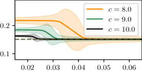
(a) $\alpha=0$

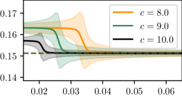
(b) $\alpha=1$

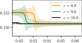
(c) $\alpha=2$

Figure 1: Adult income: Averaged test error when $a=5$ ($x$ axis is $\gamma$)

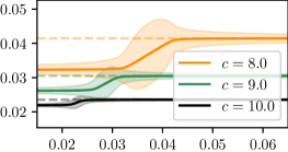
(a) $\alpha=0$

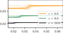
(b) $\alpha=1$

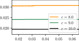
(c) $\alpha=2$

Figure 2: Adult income: Averaged test $I_{\alpha}$ when $a=5$ ($x$ axis is $\gamma$)

Figure 2 illustrate how $I_{\alpha}$ of $\bar{D}$ varies as $\gamma$ changes for each $\alpha=0,1,2$. Each graph is the average value of $I_{\alpha}$ and the shaded regions over the graphs represent 95% confidence intervals. The dotted lines represent $I_{\alpha}$ of the (empirical) risk minimizer. Every graph in Figure 2 shows that $I_{\alpha}$ increases as $\gamma$ increases: unfairness increases as the fairness constraint gets loose. For each fixed $\alpha$, as the value of $c$ increases, i.e., $r=\frac{c}{a}$ increases, we observe that the fairness degree $I_{\alpha}$ decreases since the quantity $\frac{c-a}{c}$ which is the relative difference among benefits, $(c-a,c,c+a)$, gets diminishing.

From Figures 2 and 2, we assure that fairness is achieved at the cost of accuracy. Trade-off between accuracy and fairness is more sensitive to low $\alpha$ than to high $\alpha$.

Regarding to the choice of $a$ and $c$, small $\frac{c}{a}$ may not be a good choice for stringent $\gamma$ when $\alpha=0$, since the test error for $\frac{c}{a}=\frac{8}{5}$ is relatively high compared with other values of it as in Figure 1(a). But small $\frac{c}{a}$ seems not to have such a problem when $\alpha=2$ as in Figure 1(c).

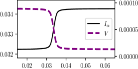
(a) Adult income

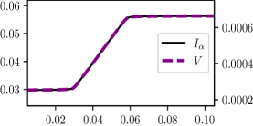
(b) COMPAS

Figure 3: $I_{\alpha}$ and $V$ ($x$ axis is $\gamma$, left $y$ axis $I_{\alpha}$, and right $y$ axis $V$)

6.2 Generalized Entropy, Between-group Term, and Equalized Odds

This subsection investigates how the between-group term $V_{\alpha}$ and equalized odds change as $\gamma$ increases. We partition the whole population into two groups, majority group ($g=0$) and minority group ($g=1$); for Adult income data set, $g=0$ corresponds to male and $g=1$ to female, and for COMPAS data set, $g=0$ corresponds to Caucasian and $g=1$ to African-American. The values of $a=5$, $c=8$, and $\alpha=1$ are used.

Figure 3 shows how between-group term $V$ changes with $\gamma$. Figure 3(a) and Figure 3(b) show the opposite behaviors of $V$ as $\gamma$ increases: in Figure 3(a), between group $V$ decreases while in Figure 3(b), $V$ increases, as $\gamma$ increases. This observation shows that regulation of $I_{\alpha}$ does not have much impact on the between-group term $V$. Note that $V$ is very small compared to $I_{\alpha}$, which is observed in experiments of the other data sets. We have found that $V$ gets large as the number of groups, $G$, gets large.

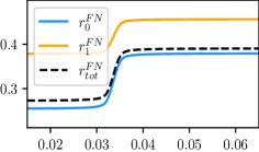
(a) Adult income

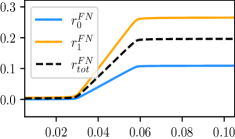
(b) COMPAS

Figure 4: $r^{FN}_{g}$ for $g\in\{0,1\}$ when $\alpha=1$ ($x$ axis is $\gamma$.)

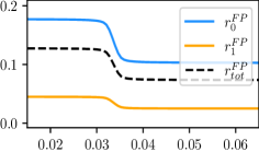
(a) Adult income

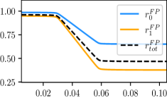
(b) COMPAS

Figure 5: $r^{FP}_{g}$ for $g\in\{0,1\}$ when $\alpha=1$ ($x$ axis is $\gamma$.)

Recall that equal opportunity is the case $r^{FN}_{0}=r^{FN}_{1}$ and equalized odds the case that $r^{FN}_{0}=r^{FN}_{1}$ and $r^{FP}_{0}=r^{FP}_{1}$. Figure 5 exhibits $r^{FN}_{g}$ and Figure 5 $r^{FP}_{g}$ for $g\in\{0,1\}$. We define $r^{FN}_{tot}$ and $r^{FP}_{tot}$ as $r^{FN}_{tot}=\mathsf{P}[h(x)=1~{}|~{}y=0]$ and $r^{FP}_{tot}=\mathsf{P}[h(x)=0~{}|~{}y=1]$. In Figure 5, the minority group of $g=1$ has higher false negative rate than the majority group of $g=0$. Also in Figure 5, the group of $g=1$ has low false positive rate than the group with $g=1$. These phenomena are observed in all of the data sets we used. Since we set $h(x)=1$ is a favorable decision to an individual both two figures show that more favorable decisions are made for group $g=0$ than for group $g=1$.

To examine how the group-level fairness definition of generalized odds (or equal opportunity) is related to $I_{\alpha}$ we consider the quantities of $|r^{FN}_{0}-r^{FN}_{1}|$ and $|r^{FP}_{0}-r^{FP}_{1}|$ in Figures 5 and 5. Note that $|r^{FN}_{0}-r^{FN}_{1}|$ is the gap between the graph of $r^{FN}_{0}$ and the graph of $r^{FN}_{1}$. In order to showing $|r^{FN}_{0}-r^{FN}_{1}|$ and $|r^{FP}_{0}-r^{FP}_{1}|$, we plot $r^{FN}_{g}-r^{FN}_{tot}$ and $r^{FP}_{g}-r^{FP}_{tot}$ in Figures 7 and 7. As $\gamma$ increases (i.e., fairness constraint gets loose), the behavior of $|r^{FN}_{0}-r^{FN}_{1}|$ of Adult income data set is opposite to that of COMPAS data set; the quantity of $|r^{FN}_{0}-r^{FN}_{1}|$ decreases in Figure 6(a) but it increases in Figure 6(b). For the quantity $|r^{FP}_{0}-r^{FP}_{1}|$, we also observe similar behaviors as in false negaive rate case. Based on these observations, controlling fairness degree by generalized entropy has no specific impact on equalized odds (or equal opportunity). The experimental results of Figures 5-7 do not violate our analysis of FERM-GE since FERM-GE controls only $I_{\alpha}$.

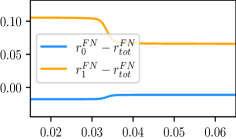
(a) Adult income

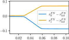
(b) COMPAS

Figure 6: $r^{FN}_{g}-r^{FN}_{tot}$ for $g\in\{0,1\}$ when $\alpha=1$ ($x$ axis is $\gamma$.)

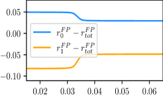
(a) Adult income

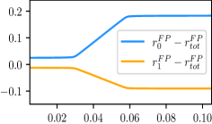
(b) COMPAS

Figure 7: $r^{FP}_{g}-r^{FP}_{tot}$ for $g\in\{0,1\}$ when $\alpha=1$ ($x$ axis is $\gamma$.)

6.3 Convergence of Empirical Errors and Generalized Entropy for Adult Income Data Set

One important performance issue is the convergence behavior of the empirical errors and values of empirical generalized entropy. We plotted the trajectories of empirical errors and empirical generalized entropy values for the adult income data set.

To investigate the convergence behaviors of time averaged empirical error and empirical $I_{\alpha}$, we plot the graphs of time averaged empirical error with time $t$ in Figure 11 and Figure 11 for given $t$, time averaged error is $\frac{1}{t}\sum_{\tau=1}^{t}\hat{h}^{(\tau)}$ where $\hat{h}^{\tau}=\arg\min_{h\in\mathcal{H}}L(h,\hat{\lambda}^{(t)})$ in Algorithm 1. All figures have time $t$ as $x$ axis and use $a=5$, and $c\in\{8,9,10\}$. Figure 11 is a closer look of Figure 11 for $1\leq t\leq 5500$. One important performance issue is the convergence behavior of the empirical errors and values of empirical generalized entropy. We plotted the trajectories of empirical errors and empirical generalized entropy values for the data sets we used. Figures 11 and 11 provides convergence behaviors of empirical error. Figures 11 and 11 provides convergence behaviors of empirical $I_{\alpha}$ of Adult income data set as $\gamma$ changes. Appedix A.2 provides figures showing how test error and test $I_{\alpha}$ changes with $\gamma$ as well as convergence behavior of empirical error and empirical $I_{\alpha}$. Appendix A.3 and Appendix A.4 provide all related figures on Law school data set and Dutch census data set, respectively.

(a) $\alpha=0$

(b) $\alpha=1$

(c) $\alpha=2$

Figure 8: Adult income: Empirical $I_{\alpha}$ trace when $a=5$ for adult income data set ($x$ axis is $\gamma$)

(a) $\alpha=0$

(b) $\alpha=1$

(c) $\alpha=2$

Figure 9: Adult income: Close look of Figure 11 for $1\leq t\leq 5500$ ($x$ axis is $\gamma$)

(a) $\alpha=0$

(b) $\alpha=1$

(c) $\alpha=2$

Figure 10: Adult income: Empirical error trace when $a=5$ ($x$ axis is $\gamma$)

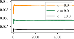
(a) $\alpha=0$

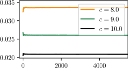
(b) $\alpha=1$

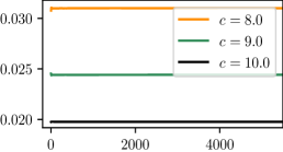
(c) $\alpha=2$

Figure 11: Adult income: Close look of Figure 11 for $1\leq t\leq 5500$ ($x$ axis is $\gamma$)

7 Summary

We theoretically and experimentally analyze a (randomized) empirical risk minimization with a fairness constraint given by generalized entropy and prove that the randomized FERM-GE is PAC learnable by proving that the true fairness degree does not deviate much from an empirical one with high probability if sample size is big enough. Regarding to the choice of $\alpha,~{}a$ and $c$, based on our analysis, a low value of $\alpha$ and a high value of $r=\frac{c}{a}(>1)$ are preferred. But if $r$ takes a too high value, it may cause a difficulty in discovering the existence of unfairness. Our experiments do not clearly show how fairness constraints affect on between-group term $V$ even though there exists a clear trade-off between $I_{\alpha}$ and accuracy. We believe it is an interesting future work to identify when $V$ has similar behaviors as $I_{\alpha}$ when $\gamma$ changes.

Appendix

Appendix A Experimental Setup and Supplementary Experiments

A.1 Data and Implementation

The data sets we used are

• Adult income data set [20] : The task is to predict if a person’s income is no less than $\$50$K per year. The population is partitioned to male, corresponding to $g=0$, and female, corresponding to $g=1$. The label value 1 indicates that the income of an individual is greater than or equal to $\$50$K per year.

• COMPAS recidivism data set [2]: Our experiments have used data samples whose race attribute is either Caucasian or African American. The task is to predict if an individual is rearrested within two years after the first arrest. The population is partitioned to Caucasian, corresponding to $g=0$, and African American attributes, corresponding to $g=1$. The label value 1 indicates no re-arrest within two years and the label value 0 indicates re-arrest within two years.

• Law school data set [29]: The task is to predict if a student passes the bar exam. The population is partitioned to male, corresponding to $g=0$, and female, corresponding to $g=1$. The label value 1 indicates that a student passes the bar exam.

• Dutch census data set [7]: The task is to predict if an individual has a prestigious occupation. The population is partitioned to male, corresponding to $g=0$, and female, corresponding to $g=1$. The label value 1 indicates that an individual has a prestigious job.

Algorithm 1 assumes the existence of an oracle $W(\lambda)$. For the implementation of an oracle, finding $\hat{h}^{(t)}=\min\arg_{h\in\mathcal{H}}L(h,\lambda)$ for $\lambda\in\{0,\lambda_{\max}\}$, in item 2 of Algorithm 1, we use thresholding [25], a simple technique to directly find the best decision threshold for a given objective from the training data and use this predict the class label for test data. a smaller probability than this threshold then it is classified as 0, otherwise as 1. Logistic regression has been used as a base classifier for thresholding. We describe below the thresholding technique used for the implementation of oracle finding $\hat{h}^{(t)}=\min\arg_{h\in\mathcal{H}}L(h,\lambda)$ for $\lambda\in\{0,\lambda_{\max}\}$, in item 2 of Algorithm 1. First, we train logistic regression with the training data set of adult. During the training, $0.5$ is the typical threshold value of logistic regression for decision: the label of an instance is predicted as 1 if its predicted probability for the positive class is higher than or equal to $\frac{1}{2}$, otherwise, its label is decided as 0. Second, we divide the interval $[0,~{}1]$ into 201 points with step size $\frac{5}{1000}$. Each point of 201 points is used a threshold and plays the role of a hypothesis. Third, for each threshold, we predict the labels of instances by comparing the threshold value and the probability of the positive class: for a give instance, if its probability of the positive class is higher or equal to the threshold value, then the label of the instance is 1, otherwise, the label is 0. Finally, to find the oracle for a given $\lambda$, we examine the value of $L(h,\lambda)$ for every $h\in\mathcal{H}$ and take $\hat{h}=\arg\min_{h\in\mathcal{H}}L(h,\lambda)$.

We use $\lambda_{max}=20,\nu=0.005$. Regarding to the value of $b_{i}=a(h(x_{i})-y_{i})+c$, we fix the value of $a$ as 5, and change the values of $c\in\{8,9,10\}$ to investigate the effect of $r=\frac{c}{a}$ on the performance for all data sets except Dutch census data set. For Dutch data set, we use $\{9,9.5,10\}$ for $c$ values.

Computational Resources All experiments were run on a server with about 250GB RAM. The server is not equipped with GPU acceleration. About 10 minutes is the run-time of an experiment to generate all related graphs for a fixed $\alpha$ and the set of $c$ values.

A.2 Supplementary Experiments on COMPAS data set

This subsection provides the plots illustrating the change of test error and test $I_{\alpha}$ obtained by the hypothesis $\bar{D}$ of Algorithm 1 in Figures 13 and 13. The behaviors of them are similar to those of adult income data set. The convergence behaviors of empirical error and $I_{\alpha}$ are shown in Figures 15-15.

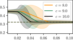
(a) $\alpha=0$

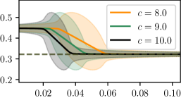
(b) $\alpha=1$

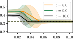
(c) $\alpha=2$

Figure 12: COMPAS: Averaged test error when $a=5$ ($x$ axis is $\gamma$)

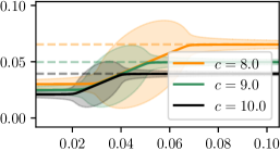
(a) $\alpha=0$

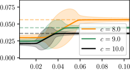
(b) $\alpha=1$

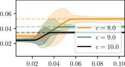
(c) $\alpha=2$

Figure 13: COMPAS: Averaged test $I_{\alpha}$ when $a=5$ ($x$ axis is $\gamma$)

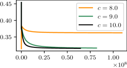
(a) $\alpha=0$

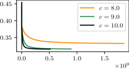
(b) $\alpha=1$

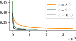
(c) $\alpha=2$

Figure 14: COMPAS: Empirical error trace when $a=5$ ($x$ axis is $\gamma$)

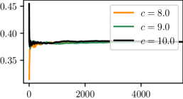
(a) $\alpha=0$

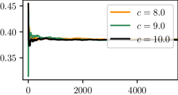
(b) $\alpha=1$

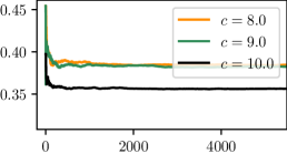
(c) $\alpha=2$

Figure 15: COMPAS: Close look of Figure 15 for $1\leq t\leq 5500$ ($x$ axis is $\gamma$)

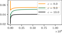
(a) $\alpha=0$

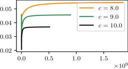
(b) $\alpha=1$

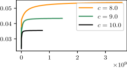
(c) $\alpha=2$

Figure 16: COMPAS: Empirical $I_{\alpha}$ trace when $a=5$ ($x$ axis is $\gamma$)

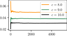
(a) $\alpha=0$

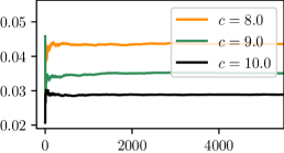
(b) $\alpha=1$

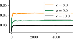
(c) $\alpha=2$

Figure 17: COMPAS: Close look of Figure 17 for $1\leq t\leq 5500$ ($x$ axis is $\gamma$)

A.3 Experiments on The Dutch Census Data set

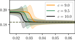
(a) $\alpha=0$

(b) $\alpha=1$

(c) $\alpha=2$

Figure 18: Dutch census: Averaged test error when $a=5$ ($x$ axis is $\gamma$)

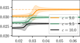
(a) $\alpha=0$

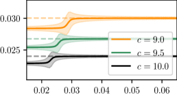
(b) $\alpha=1$

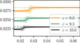
(c) $\alpha=2$

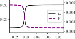
Figure 19: Dutch census: Averaged test $I_{\alpha}$ when $a=5$($x$ axis is $\gamma$)

Figure 20: Dutch Census: $I_{\alpha}$ and $V$ when $\alpha=1$

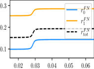
(a) $r^{FN}_{g}$

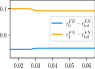
(b) $r^{FN}_{g}-|r^{FN}_{tot}$

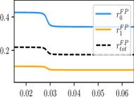
(c) $r^{FP}_{g}$

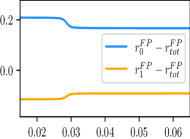
(d) $r^{FP}_{g}-r^{FP}_{tot}$

Figure 21: Dutch Census: $r^{FN}_{g}$ and $r^{FP}_{g}$ when $\alpha=1$

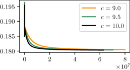
(a) $\alpha=0$

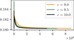
(b) $\alpha=1$

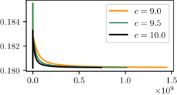
(c) $\alpha=2$

Figure 22: Dutch census: Empirical error trace when $a=5$ ($x$ axis is $\gamma$)

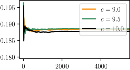
(a) $\alpha=0$

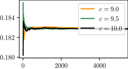
(b) $\alpha=1$

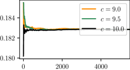
(c) $\alpha=2$

Figure 23: Dutch census: Close look of Figure 23 for $1\leq t\leq 5500$ ($x$ axis is $\gamma$)

(a) $\alpha=0$

(b) $\alpha=1$

(c) $\alpha=2$

Figure 24: Dutch census: Empirical $I_{\alpha}$ trace when $a=5$ ($x$ axis is $\gamma$)

(a) $\alpha=0$

(b) $\alpha=1$

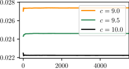
(c) $\alpha=2$

Figure 25: Dutch census: Close look of Figure 25 for $1\leq t\leq 5500$ ($x$ axis is $\gamma$)

A.4 Experiments on Law School Admissions Data Set

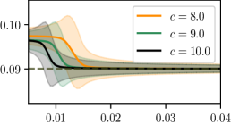
(a) $\alpha=0$

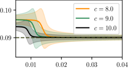
(b) $\alpha=1$

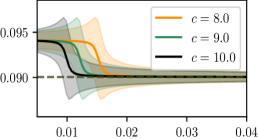
(c) $\alpha=2$

Figure 26: Law school: Averaged test error when $a=5$ ($x$ axis is $\gamma$)

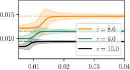
(a) $\alpha=0$

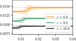
(b) $\alpha=1$

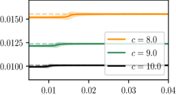
(c) $\alpha=2$

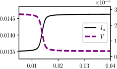
Figure 27: Law school: Averaged test $I_{\alpha}$ when $a=5$ ($x$ axis is $\gamma$)

Figure 28: Law school: $I_{\alpha}$ and $V$ when $\alpha=1$

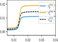
(a) $r^{FN}_{g}$

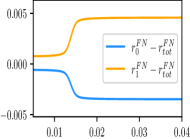
(b) $r^{FN}_{g}-r^{FN}_{tot}$

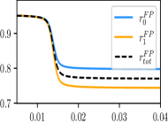
(c) $r^{FP}_{g}$

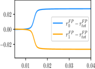
(d) $r^{FP}_{g}-r^{FP}_{tot}$

Figure 29: Law school: $r^{FN}_{g}$ and $r^{FP}_{g}$ when $\alpha=1$

(a) $\alpha=0$

(b) $\alpha=1$

(c) $\alpha=2$

Figure 30: Law school: Empirical $I_{\alpha}$ trace when $a=5$ ($x$ axis is $\gamma$)

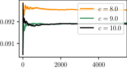
(a) $\alpha=0$

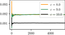
(b) $\alpha=1$

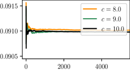
(c) $\alpha=2$

Figure 31: Law school: Close look of Figure 31 for $1\leq t\leq 5500$ ($x$ axis is $\gamma$)

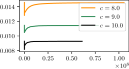
(a) $\alpha=0$

(b) $\alpha=1$

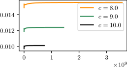
(c) $\alpha=2$

Figure 32: Law school: Empirical $I_{\alpha}$ trace when $a=5$ ($x$ axis is $\gamma$)

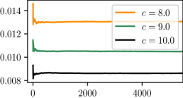
(a) $\alpha=0$

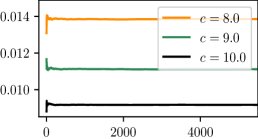
(b) $\alpha=1$

(c) $\alpha=2$

Figure 33: Law school: Close look of Figure 33 for $1\leq t\leq 5500$ ($x$ axis is $\gamma$)

Appendix B A Computation Example of Additive Decomposability

We explain with an example how to compute generalized entropy $I_{\alpha}(\bm{b};n)$ and check additive decomposability, (5),

$$I(\bm{b}^{1},...,\bm{b}^{G};n)=\sum_{g}w_{g}^{G}(\bm{\mu},\bm{n})I(\bm{b}^{g};n_{g})+V$$

We set $\alpha=1$ in this example and use $I$ instead of $I_{\alpha}$. Consider 10 individuals $\{\bm{x}_{1},\bm{x}_{2},...,\bm{x}_{10}\}$. There are two groups $X^{1}$ and $X^{2}$ such that $X^{1}=\{\bm{x}_{1},...\bm{x}_{5}\}$ and $X^{2}=\{\bm{x}_{6},..,\bm{x}_{10}\}$. The true label is denoted by $y_{i}$ and predicted label by $h(\bm{x}_{i})$. The benefit value $b_{i}$ is defined by $b_{i}=h(\bm{x}_{i})-y_{i}+3$ for a given classifier $h$. Then $\bm{b}=(\bm{b}^{1},\bm{b}^{2})=(b_{\bm{x}_{1}},...,b_{\bm{x}_{10}})$. For groups $X^{1}$ and $X^{2}$, we have $\bm{b}^{1}=(b_{1},...,b_{5})$ and $\bm{b}^{2}=(b_{6},...,b_{10})$. For this special case of groups $X^{1}$ and $X^{2}$, the Axiom 4 (the additivie decomposability) is written by

$$I(b_{1},...,b_{10};10)=w_{1}I(b_{1},...,b_{5};5)+w_{2}I(b_{6},...,b_{10};5)+V$$

if we use a simple notation $w_{i}$ instead of $w^{G}_{i}(\bm{\mu},\bm{n})$.

Note that $I(b_{1},...,b_{5};5)$ is the generalized entropy for group $X^{1}$ whose members have benefits $b_{1},b_{2},...,b_{5}$. Similarly $I(b_{6},...,b_{10})$ is the generalized entropy for group $X^{2}$ with the benefits, $b_{6},b_{7},...,b_{10}$. Consider a classifier $h_{1}$ whose prediction $h_{1}(x_{i})$ is given in Table 1. We will use superscript $h_{1}$ to make clear which classifier is used, if necessary.

Table 1: Classifier $h_{1}$

Group	$X^{1}$					$X^{2}$
Individuals $\bm{x}_{i}$	$\bm{x}_{1}$	$\bm{x}_{2}$	$\bm{x}_{3}$	$\bm{x}_{4}$	$\bm{x}_{5}$	$\bm{x}_{6}$	$\bm{x}_{7}$	$\bm{x}_{8}$	$\bm{x}_{9}$	$\bm{x}_{10}$
$y_{i}$: true label	1	1	1	1	0	1	0	1	1	1
$h_{1}(x_{i})$: predicted label	1	0	1	0	1	1	1	1	1	0
C, FP, FN	C	FN	C	FN	FP	C	FP	C	C	FN
$b_{i}$	3	2	3	2	4	3	4	3	3	2

Let $n_{C}$ be the number of correct labels, $n_{FP}$ the number of false positive labels, and $n_{FN}$ the number of false negative labels. Then the average of the value $b_{i}$’s and generalized entropy $I^{h_{1}}(\bm{b}_{h_{1}};10)$ for the whole population are

$$\mu^{h_{1}} = \frac{1}{10}\sum_{i=1}^{10}b_{i}=\frac{1}{10}\Big{(}n_{C}*3+n_{FP}*4+n_{FN}*2\Big{)}=\frac{29}{10},$$

$$I^{h_{1}}(\bm{b}_{h_{1}};10) = \frac{1}{10}\Big{(}n_{C}*\frac{3}{\mu^{h_{1}}}\ln\frac{3}{\mu^{h_{1}}}+n_{FP}*\frac{4}{\mu^{h_{1}}}\ln\frac{4}{\mu^{h_{1}}}+n_{FN}*\frac{2}{\mu^{h_{1}}}\ln\frac{2}{\mu^{h_{1}}}\Big{)}$$

$$= 0.0848.$$

Let’s compute the generalized entropy of group $X^{1}$ that has five individuals $x_{1},..,x_{5}$. Consider the average of $b_{i}$ for the individuals of $X^{1}$, i.e.,

$$\mu^{h_{1}}(X^{1})=\frac{1}{5}\sum_{i=1}^{5}b_{i}=\frac{2*3+1*4+2*2}{5}=\frac{14}{5}.$$

The generalized entropy for $X^{1}$ is

$$I^{h_{1}}(b_{x_{1}},..,b_{x_{5}};5)$$

$$= \frac{1}{5}\Big{(}2*\frac{3}{\mu^{h_{1}}(X^{1})}\ln\frac{3}{\mu^{h_{1}}(X^{1})}+1*\frac{4}{\mu^{h_{1}}(X^{1})}\ln\frac{4}{\mu^{h_{1}}(X^{1})}+2*\frac{2}{\mu^{h_{1}}(X^{1})}\ln\frac{2}{\mu^{h_{1}}(X^{1})}\Big{)}$$

$$= 0.0990.$$

Similarly, for group $X^{2}=\{x_{6},...,x_{10}\}$, we have $\mu^{h_{1}}(X^{2})=3$ and $I^{h_{1}}(b_{x_{6}},...,b_{x_{10}};5)=0.0680$ Now we can find $w^{h_{1}}_{1}=\frac{n_{1}}{n}\frac{\mu^{h_{1}}(X^{1})}{\mu}=\frac{5}{10}\frac{\frac{14}{5}}{\frac{29}{10}}=\frac{14}{29}$ and $w^{h_{1}}_{2}=\frac{5}{10}\frac{3}{\frac{29}{10}}=\frac{15}{29}$.

Now consider $V$. To compute $V$, we consider two groups, $\{j_{1},j_{2},...,j_{5}\}$ and $\{j_{6},j_{7},...,j_{10}\}$, and the benefit of the individuals which is such that $b_{j_{1}}=b_{j_{2}}=..=b_{j_{5}}=\mu(b_{j_{1}},..,b_{j_{5}})=\frac{14}{5}$ and $b_{j_{6}}=b_{j_{7}}=..=b_{j_{10}}=\mu(b_{j_{6}},...,b_{j_{10}})=3$. Note that every member in $\{j_{1},..,j_{5}\}$ have the identical benefit $\frac{14}{5}$ and every member member in $\{j_{6},..,j_{10}\}$ have identical benefit $3$. Definitely the average value of the benefit for the individuals $j_{1},...j_{10}$ is $\mu^{h_{1}}$. Hence

$$V^{h_{1}} = I(b_{j_{1}},..,b_{j_{10}};10)$$

$$= \frac{1}{10}\Big{(}5*\frac{\mu(b_{j_{1}},..,b_{j_{5}})}{\mu^{h_{1}}}\ln\frac{\mu(b_{j_{1}},..,b_{j_{5}})}{\mu^{h_{1}}}+5*\frac{\mu(b_{j_{6}},...,b_{j_{10}})}{\mu^{h_{1}}}\ln\frac{\mu(b_{j_{6}},...,b_{j_{10}})}{\mu^{h_{1}}}\Big{)}$$

$$= \frac{1}{10}\Big{(}5*\frac{14/5}{29/10}\ln\frac{14/5}{29/10}+5*\frac{3}{29/10}\ln\frac{3}{29/10}\Big{)}$$

$$= 0.0018.$$

Indeed we can check that $I(b_{x_{1}},...,b_{x_{10}};10)=w_{1}I^{h_{1}}(X^{1};5)+w_{2}I^{h_{1}}(X^{2};5)+V^{h_{1}}$ with the values of $w_{1}^{h_{1}}I^{h_{1}}(X^{1};5)=0.0478$, $w_{2}^{h_{1}}I^{h_{1}}(X^{2};5)=0.0352$, and $V^{h_{1}}=0.0018$.

Appendix C Proof of Theorem 4.2

Obviously Axioms 1, 3^′, and 7 hold.

Theorem C.1 ( Jensen’s Inequality, [24]).

Let $Q$ be a probability distribution on $\mathcal{X}$ and dQ the probability density function of $Q$. If $b$ is a real function with $\int_{\mathcal{X}}|b(\bm{x})|dQ$, $a_{1}<b(\bm{x})<a_{2}$ for all $\bm{x}\in\mathcal{X}$, and $\phi$ is convex on $(a_{1},a_{2})$, then

$$\phi\Big{(}\int_{\mathcal{X}}b(\bm{x})dQ\Big{)}\leq\int_{\mathcal{X}}\phi\big{(}b(\bm{x})\big{)}dQ.$$

C.1 Proof for Axiom $\bm{2^{\prime}}$

Note that $f_{\alpha}(x)$ is convex over for all $\alpha\in[0,\infty)$. We will show that $I_{1}(b,\mathcal{X},P_{x})\geq 0$ for $\alpha=1$: recall that $b(\bm{x})=a(h(\bm{x})-y)+c$.

$$I_{1}(b,\mathcal{X},P_{x}) = \int_{\mathcal{X}}\frac{b(\bm{x})}{\mu}\ln\Big{(}\frac{b(\bm{x})}{\mu}\Big{)}dP_{x}$$

$$= \frac{1}{\mu}\int_{\mathcal{X}}b(\bm{x})\ln b(\bm{x})dP_{x}-\frac{1}{\mu}\int_{\mathcal{X}}\Big{(}b(\bm{x})\ln\mu\Big{)}dP_{x}$$

$$= \frac{1}{\mu}\Big{(}\int_{\mathcal{X}}b(\bm{x})\ln b(\bm{x})dP_{x}-\mu\ln\mu\Big{)}$$

$$\geq \frac{1}{\mu}\Big{[}f_{1}\Big{(}\int_{\mathcal{X}}b(\bm{x})\ln b(\bm{x})dP_{x}\Big{)}-\mu\ln\mu\Big{]}$$

$$\geq 0.$$

The first inequality holds by Jensen’s inequality since $b(\bm{x})$ is bounded and $f_{1}(x)$ is convex. In a similar way, we can show that $I_{\alpha}(b,\mathcal{X},P_{x})\geq 0$ for $\alpha\neq 1$.

C.2 Proof for Axiom 4^′ (Additive decomposability)

Recall that $\upsilon(\bm{x})=\sum_{g=1}^{G}\mu_{g}\mathds{1}\{\bm{x}\in\mathcal{X}^{g}\}$ and $m_{g}=P_{x}(\mathcal{X}^{g})$. For any $A\subset\mathcal{X}^{g}$, we have $P_{x}^{g}(A)=\frac{P_{x}(A)}{P_{x}(\mathcal{X}^{g})}=\frac{P_{x}(A)}{m_{g}}$. Hence $P_{x}^{g}=\frac{P_{x}}{m_{g}}$ and $dP_{x}=m_{g}dP_{x}^{g}$ for all $g$.

Lemma C.2.

$$\mathsf{E}[\upsilon(\bm{x})]=\mu=\sum_{g=1}^{G}m_{g}\mu_{g}.$$

Proof.

Since $\mathcal{X}$ is a disjoint union of $\mathcal{X}^{g}$ for $1\leq g\leq G$, we have

$$\mu=\int_{\mathcal{X}}b(\bm{x})dP_{x}=\int_{\dot{\bigcup}\mathcal{X}^{g}}b(\bm{x})dP_{x}=\sum_{g=1}^{G}\int_{\mathcal{X}^{g}}b(\bm{x})dP_{x}$$ (24)

where $\dot{\bigcup}$ means a disjoint union. Then

$$\sum_{g=1}^{G}\int_{\mathcal{X}^{g}}b(\bm{x})dP_{x}=\sum_{g=1}^{G}m_{g}\int_{\mathcal{X}^{g}}{b}(\bm{x})dP_{x}^{g}=\sum_{g=1}^{G}m_{g}\mu_{g}.$$ (25)

Combining (24) and (25), we have $\mu=\sum_{g=1}^{G}m_{g}\mu_{g}$. Consider $\mathsf{E}[\upsilon(\bm{x})]$;

$$\mathsf{E}[\upsilon(\bm{x})]=\mathsf{E}\big{[}\sum_{g=1}^{G}\mu_{g}\mathds{1}\{\bm{x}\in\mathcal{X}^{g}\}\big{]}=\sum_{g=1}^{G}\mu_{g}\mathsf{E}\big{[}\mathds{1}\{\bm{x}\in\mathcal{X}^{g}\}\big{]}=\sum_{g=1}^{G}m_{g}\mu_{g}=\mu.$$

∎

Lemma C.3.

For $\alpha\in[0,\infty)$, it holds that

$$I_{\alpha}(b,\mathcal{X},P_{x}) = \sum_{g=1}^{G}m_{g}f_{\alpha}\Big{(}\frac{\mu_{g}}{\mu}\Big{)}.$$

Proof.

Since $\mathcal{X}=\dot{\bigcup}\mathcal{X}^{g}$, for each $\bm{x}\in\mathcal{X}$, there is a unique $g$ such that $\bm{x}\in\mathcal{X}^{g}$. Therefore

$$\upsilon(\bm{x})=\sum_{i=1}^{G}\mu_{i}\mathds{1}\{\bm{x}\in\mathcal{X}^{i}\}=\mu_{g}\qquad\mbox{for }\bm{x}\in\mathcal{X}^{g}.$$ (26)

Consider $I_{\alpha}(\upsilon,\mathcal{X},P_{x})$;

$$I_{\alpha}(\upsilon,\mathcal{X},P_{x}) = \int_{\mathcal{X}}f_{\alpha}\Big{(}\frac{\upsilon(\bm{x})}{\mathsf{E}[\upsilon(\bm{x})]}\Big{)}dP_{x}$$

$$= \int_{\mathcal{X}}f_{\alpha}\Big{(}\frac{\upsilon(\bm{x})}{\mu}\Big{)}dP_{x}\qquad(\mbox{by Lemma \ref{lemma:Eupsilon(x)}})$$

$$= \sum_{g=1}^{G}\int_{\mathcal{X}^{g}}f_{\alpha}\Big{(}\frac{\mu_{g}}{\mu}\Big{)}dP_{x}\qquad(\mbox{by }(\ref{eqn:upsilon(x)}))$$

$$= \sum_{g=1}^{G}m_{g}f_{\alpha}\Big{(}\frac{\mu_{g}}{\mu}\Big{)}.$$

∎

1. $\alpha=1$
   Using $\mathcal{X}=\dot{\bigcup}\mathcal{X}^{g}$, we have

   $$I_{\alpha}(b,\mathcal{X},P_{x}) = \int_{\dot{\bigcup}\mathcal{X}^{g}}\frac{b(\bm{x})}{\mu}\ln\frac{b(\bm{x})}{\mu}dP_{x}$$ (27)

   $$= \sum_{g=1}^{G}\int_{\mathcal{X}^{g}}\frac{b(\bm{x})}{\mu}\ln\frac{b(\bm{x})}{\mu}dP_{x}$$

   $$= \sum_{g=1}^{G}m_{g}\int_{\mathcal{X}^{g}}\frac{{b}(\bm{x})}{\mu}\ln\frac{{b}(\bm{x})}{\mu}dP_{x}^{g}.$$

   Since $\frac{{b}(\bm{x})}{\mu}\ln\frac{{b}(\bm{x})}{\mu}=\frac{\mu_{g}}{\mu}\frac{{b}(\bm{x})}{\mu_{g}}\Big{(}\ln\frac{{b}(\bm{x})}{\mu_{g}}+\ln\frac{\mu_{g}}{\mu}\Big{)}$, we have

   $$\int_{\mathcal{X}^{g}}\frac{{b}(\bm{x})}{\mu}\ln\frac{{b}(\bm{x})}{\mu}dP_{x}^{g} = \frac{\mu_{g}}{\mu}\Big{(}\int_{\mathcal{X}^{g}}\frac{{b}(\bm{x})}{\mu_{g}}\ln\frac{{b}(\bm{x})}{\mu_{g}}dP_{x}^{g}+\ln\frac{\mu_{g}}{\mu}\int_{\mathcal{X}^{g}}\frac{{b}(\bm{x})}{\mu_{g}}dP_{x}^{g}\Big{)}$$ (28)

   $$= \frac{\mu_{g}}{\mu}\Big{(}I_{\alpha}(b|_{\mathcal{X}^{g}},\mathcal{X}_{g},P_{x}^{g})+\ln\frac{\mu_{g}}{\mu}\Big{)}\quad\big{(}\because\mu_{g}=\int_{\mathcal{X}_{g}}{b}(\bm{x})dP_{x}^{g}\big{)}\qquad~{}~{}~{}$$

   By (28), equation (27) becomes

   $$I_{\alpha}(b,\mathcal{X},P_{x}) = \sum_{g=1}^{G}m_{g}\frac{\mu_{g}}{\mu}\Big{(}I_{\alpha}(b|_{\mathcal{X}^{g}},\mathcal{X}_{g},P_{x}^{g})+\ln\frac{\mu_{g}}{\mu}\Big{)}$$

   $$= \sum_{g=1}^{G}m_{g}\frac{\mu_{g}}{\mu}I_{\alpha}(b|_{\mathcal{X}^{g}},\mathcal{X}_{g},P_{x}^{g})+\sum_{g=1}^{G}m_{g}\frac{\mu_{g}}{\mu}\ln\frac{\mu_{g}}{\mu}$$

   By Lemma C.3, we have

   $$I_{1}(\upsilon,\mathcal{X},P_{x})~{}=~{}\sum_{g=1}^{G}m_{g}f_{1}\Big{(}\frac{\mu_{g}}{\mu}\Big{)}~{}=~{}\sum_{g=1}^{G}m_{g}\frac{\mu_{g}}{\mu}\ln\frac{\mu_{g}}{\mu}.$$

   Hence we have proved that the extended generalized entropy has the additive decomposable property when $\alpha=1$.

2. $\alpha=0$
   This case can be shown similarly as in the case $\alpha=1$. So we omit the detail of it.

3. $\alpha\neq 0,1$ (and $0<\alpha<\infty$)
   

   $$I_{\alpha}(b,\mathcal{X},P_{x}) = \frac{1}{\alpha(\alpha-1)}\int_{\mathcal{X}}\Big{[}\Big{(}\frac{b(\bm{x})}{\mu}\Big{)}^{\alpha}-1\Big{]}dP_{x}$$ (29)

   $$= \frac{1}{\alpha(\alpha-1)}\sum_{g=1}^{G}\int_{\mathcal{X}^{g}}\Big{[}\Big{(}\frac{b(\bm{x})}{\mu}\Big{)}^{\alpha}-1\Big{]}dP_{x}$$

   $$= \frac{1}{\alpha(\alpha-1)}\sum_{g=1}^{G}m_{g}\int_{\mathcal{X}^{g}}\Big{[}\Big{(}\frac{b(\bm{x})}{\mu}\Big{)}^{\alpha}-1\Big{]}dP_{x}^{g}$$

   Since $\Big{(}\frac{b(\bm{x})}{\mu}\Big{)}^{\alpha}-1=\Big{(}\frac{\mu_{g}}{\mu}\Big{)}^{\alpha}\Big{[}\Big{(}\frac{b(\bm{x})}{\mu_{g}}\Big{)}^{\alpha}-1\Big{]}+\Big{(}\frac{\mu_{g}}{\mu}\Big{)}^{\alpha}-1,$ we have

   $$\int_{\mathcal{X}^{g}}\Big{[}\Big{(}\frac{b(\bm{x})}{\mu_{g}}\Big{)}^{\alpha}-1\Big{]}dP_{x}^{g} = \int_{\mathcal{X}^{g}}\Big{(}\frac{\mu_{g}}{\mu}\Big{)}^{\alpha}\Big{[}\Big{(}\frac{b(\bm{x})}{\mu}\Big{)}^{\alpha}-1\Big{]}dP_{x}^{g}+\int_{\mathcal{X}^{g}}\Big{[}\Big{(}\frac{\mu_{g}}{\mu}\Big{)}^{\alpha}-1\Big{]}dP_{x}^{g}$$

   $$= \Big{(}\frac{\mu_{g}}{\mu}\Big{)}^{\alpha}\alpha(\alpha-1)I_{\alpha}(b|_{\mathcal{X}^{g}},\mathcal{X}^{g},P_{x}^{g})+\Big{(}\frac{\mu_{g}}{\mu}\Big{)}^{\alpha}-1$$

   $$\qquad(\mbox{because }\mu_{g}=\int_{\mathcal{X}^{g}}b(\bm{x})dP_{x}^{g}).$$

   By (29), we have

   $$I_{\alpha}(b,\mathcal{X},P_{x}) = \sum_{g=1}^{G}m_{g}\Big{(}\frac{\mu_{g}}{\mu}\Big{)}^{\alpha}I_{\alpha}(b|_{\mathcal{X}^{g}},\mathcal{X}^{g},P_{x}^{g})~{}+~{}\frac{1}{\alpha(\alpha-1)}\sum_{g=1}^{G}m_{g}\Big{[}\Big{(}\frac{\mu_{g}}{\mu}\Big{)}^{\alpha}-1\Big{]}$$

   $$= \sum_{g=1}^{G}m_{g}\Big{(}\frac{\mu_{g}}{\mu}\Big{)}^{\alpha}I_{\alpha}(b|_{\mathcal{X}^{g}},\mathcal{X}^{g},P_{x}^{g})~{}+\sum_{g=1}^{G}m_{g}f_{\alpha}\Big{(}\frac{\mu_{g}}{\mu}\Big{)}$$

   $$= \sum_{g=1}^{G}m_{g}\Big{(}\frac{\mu_{g}}{\mu}\Big{)}^{\alpha}I_{\alpha}(b|_{\mathcal{X}^{g}},\mathcal{X}^{g},P_{x}^{g})~{}+I_{\alpha}(b,\mathcal{X},P_{x})\qquad(\mbox{By Lemma \ref{lemma:V_in_gen_entropy}}).$$

C.3 Proof for Axiom $\bm{6^{\prime}}$

It can be easily checked that $P_{x}(M_{i})=P_{x}(M_{j})$ from the assumption that $\mathsf{E}[b(\bm{x})]=\mathsf{E}[\tilde{b}(\bm{x})]=\mu$. We need a simple property of a real-valued differentiable convex function, which is stated in the Lemma below.

Lemma C.4.

[3] Suppose that $f:\mathbb{R}\rightarrow\mathbb{R}$ is a differentiable real-valued function. Then $f$ is convex if and only if

$$f(\bm{x}_{2})\geq f(\bm{x}_{1})+f^{\prime}(\bm{x}_{1})^{T}(\bm{x}_{2}-\bm{x}_{1})$$

Note that $f_{\alpha}(x)$ in (12) is a real-valued convex function defined on $\mathbb{R}$ for all $\alpha\in[0,\infty)$. Therefore Lemma C.4 holds and moreover $f^{\prime}_{\alpha}(x_{2})>f^{\prime}_{\alpha}(x_{1})$ if $x_{2}>x_{1}$.

We will show that $I_{\alpha}(b,\mathcal{X},P_{x})-I_{\alpha}(\tilde{b},\mathcal{X},P_{x})\geq 0$.

$$I_{\alpha}(b,\mathcal{X},P_{x})-I_{\alpha}(\tilde{b},\mathcal{X},P_{x})$$

$$= \int_{\mathcal{X}}f_{\alpha}\Big{(}\frac{b(\bm{x})}{\mu}\Big{)}dP_{x}-\int_{\mathcal{X}}f_{\alpha}\Big{(}\frac{\tilde{b}(\bm{x})}{\mu}\Big{)}dP_{x}$$

$$= \int_{M_{i}\cup M_{j}}f_{\alpha}\Big{(}\frac{b(\bm{x})}{\mu}\Big{)}dP_{x}-\int_{M_{i}\cup M_{j}}f_{\alpha}\Big{(}\frac{\tilde{b}(\bm{x})}{\mu}\Big{)}dP_{x}$$

$$= \int_{M_{i}}f_{\alpha}\Big{(}\frac{b(\bm{x})}{\mu}\Big{)}dP_{x}+\int_{M_{j}}f_{\alpha}\Big{(}\frac{b(\bm{x})}{\mu}\Big{)}dP_{x}-\Big{[}\int_{M_{i}}f_{\alpha}\Big{(}\frac{\tilde{b}(\bm{x})}{\mu}\Big{)}dP_{x}+\int_{M_{j}}f_{\alpha}\Big{(}\frac{\tilde{b}(\bm{x})}{\mu}\Big{)}dP_{x}\Big{]}$$

$$= \int_{M_{i}}f_{\alpha}\Big{(}\frac{b(\bm{x})}{\mu}\Big{)}dP_{x}+\int_{M_{j}}f_{\alpha}\Big{(}\frac{b(\bm{x})}{\mu}\Big{)}dP_{x}-\Big{[}\int_{M_{i}}f_{\alpha}\Big{(}\frac{b(\bm{x})-\delta}{\mu}\Big{)}dP_{x}+\int_{M_{j}}f_{\alpha}\Big{(}\frac{b(\bm{x})+\delta}{\mu}\Big{)}dP_{x}\Big{]}$$

$$= \int_{M_{i}}\Big{[}f_{\alpha}\Big{(}\frac{b(\bm{x})}{\mu}\Big{)}-f_{\alpha}\Big{(}\frac{b(\bm{x})-\delta}{\mu}\Big{)}\Big{]}dP_{x}-\int_{M_{j}}\Big{[}f_{\alpha}\Big{(}\frac{b(\bm{x})+\delta}{\mu}\Big{)}-f_{\alpha}\Big{(}\frac{b(\bm{x})}{\mu}\Big{)}\Big{]}dP_{x}$$

$$> \int_{M_{i}}f^{\prime}_{\alpha}\Big{(}\frac{b(\bm{x})-\delta}{\mu}\Big{)}\delta dP_{x}-\int_{M_{j}}f^{\prime}_{\alpha}\Big{(}\frac{b(\bm{x})}{\mu}\Big{)}\delta dP_{x}\qquad(\mbox{by }Lemma\ref{lemma:convex})$$

$$= \delta P_{x}(M_{i})\Big{[}f^{\prime}_{\alpha}\Big{(}\frac{b(\bm{x})-\delta}{\mu}\Big{)}-f^{\prime}_{\alpha}\Big{(}\frac{b(\bm{x})}{\mu}\Big{)}\Big{]}$$

$$\geq 0\qquad(\mbox{because $P_{x}(M_{i})=P_{x}(M_{j})$ and the convexity of $f_{\alpha}$}).$$

Appendix D Proof of Theorem 4.4

Theorem D.1 (Mean Value Theorem).

Let $f$ be a continuous real-valued function on $[a,b]$. If $f$ is differentiable in $(a,b)$, then there exists some $x\in(a,b)$ such that

$$f(b)-f(a)=(b-a)f^{\prime}(x).$$

Theorem D.2 (McDiarmid’s Inequality).

Let $X_{1},X_{2},\ldots,X_{n}$ be i.i.d random variables defined on $\mathcal{X}$. Consider a function $\phi:\mathcal{X}^{n}\rightarrow$. If for all $1\leq i\leq n$ and all $\bm{x}_{1},\ldots,\bm{x}_{i-1},\bm{x}_{i+1},\ldots,\bm{x}_{n}\in\mathcal{X}$, the function satisfies

$$\sup_{\bm{x}\in V}\phi(\bm{x}_{1},\ldots,\bm{x}_{i-1},\bm{x},\bm{x}_{i+1},\ldots,\bm{x}_{n})-\inf_{\bm{x}\in V}\phi(\bm{x}_{1},\ldots,\bm{x}_{i-1},\bm{x},\bm{x}_{i+1},\ldots,\bm{x}_{n})\leq q_{i}.$$ (30)

with $q_{i}>0$, then

$$\mathsf{P}\Big{[}\Big{|}\phi(X_{1},\ldots,X_{n})-\mathsf{E}[\phi(X_{1},\ldots,X_{n})]\Big{|}\geq\varepsilon\Big{]}\leq 2\exp\Big{(}\frac{-2\varepsilon^{2}}{\sum_{i=1}^{n}q_{i}^{2}}\Big{)}.$$

Lemma D.3.

The function $f(x)=x\ln x$ is non-negative, increasing and convex for $x\geq\frac{1}{e}$.

Proof.

Obviously $f(x)\geq 0$ for $x\geq 1$. The first derivative is $f^{\prime}(x)=\ln x+1>0$ for $x\geq 1$; $f(x)$ is increasing over $x\geq\frac{1}{e}$. The second derivative is $f^{\prime\prime}(x)=\frac{1}{x}>0$ for $x>0$: $f(x)$ is convex over $x\geq\frac{1}{e}$. ∎

For the purpose of distinguishing $b_{i}$ and $b(\bm{x})$ and simple notation, we use $\beta$ for $b(\bm{x})$ instead of $b(\bm{x})$: for example, $\mathsf{E}[\beta]$ stands for $\mathsf{E}[b(\bm{x})]$ and $\mathsf{E}[\beta\ln(\beta)]$ for $\mathsf{E}[b(\bm{x})\ln b(\bm{x})]$. Moreover, we let $\omega=\mathsf{E}[b(\bm{x})]=\mathsf{E}[\beta]$.

D.1 When $\alpha=0$

Recall that $\mu=\frac{1}{n}\sum_{i=1}^{n}b_{i}$ where $b_{i}=a(h(\bm{x}_{i})-y_{i})+c$ with $c>a>0$ and $c-a\geq 1$. Consider $\Big{|}I_{0}(h,P)-I_{0}(\bm{b};n)\Big{|}$:

$$\Big{|}I_{0}(h,P)-I_{0}(\bm{b};n)\Big{|} = \Big{|}\int_{\mathcal{X}}\ln\Big{(}\frac{\mathsf{E}[b(\bm{x})]}{b(\bm{x})}\Big{)}dP_{x}-\frac{1}{n}\sum_{i=1}^{n}\ln\frac{\mu}{b_{i}}\Big{|}$$ (31)

$$= \Big{|}\ln\mathsf{E}[\beta]-\mathsf{E}[\ln\beta]-(\ln\mu-\frac{1}{n}\sum_{i=1}^{n}\ln b_{i}\Big{)}\Big{|}$$

$$= \Big{|}\ln\mathsf{E}[\beta]-\ln\mu-\Big{(}\mathsf{E}[\ln\beta]-\frac{1}{n}\sum_{i=1}^{n}\ln b_{i}\Big{)}\Big{|}$$

$$\leq \Big{|}\ln\mathsf{E}[\beta]-\ln\mu\Big{|}+\Big{|}\mathsf{E}[\ln\beta]-\frac{1}{n}\sum_{i=1}^{n}\ln b_{i}\Big{|}$$

Let $M=\max(\mu,\mathsf{E}[\beta])$ and $m=\min(\mu,\mathsf{E}[\beta])$. Then

$$\Big{|}\ln\mathsf{E}[\beta]-\ln\mu\Big{|} = \ln\Big{(}1+\frac{M-m}{m}\Big{)}$$ (32)

$$\leq \frac{M-m}{m}~{}~{}\Big{(}=\frac{|\mathsf{E}[\beta]-\mu|}{m}\Big{)}\qquad(\mbox{since }\ln(1+x)<x)$$

$$\leq \frac{|\mathsf{E}[\beta]-\mu|}{c-a}\qquad(\mbox{since }\mu\geq c-a,~{}\mathsf{E}[\beta]\geq c-a).$$ (33)

Then, (31) becomes

$$\Big{|}I_{0}(h,P)-I_{0}(\bm{b};n)\Big{|}\leq\frac{|\mathsf{E}[\beta]-\mu|}{c-a}+\Big{|}\mathsf{E}[\ln\beta]-\frac{1}{n}\sum_{i=1}^{n}\ln b_{i}\Big{|}.$$ (34)

Lemma D.4.

With probability at least $1-\frac{\delta}{2}$, we have

$$\Big{|}\mathsf{E}[\beta]-\mu\Big{|} < a\sqrt{\frac{2}{n}\ln\frac{4}{\delta}}.$$ (35)

Proof.

For $|\mathsf{E}[\beta]-\mu|$, we will apply McDiarmid’s Inequality to the function $\phi(\bm{x}_{1},\ldots,\bm{x}_{n})=\frac{1}{n}\sum_{i=1}^{n}b(\bm{x}_{i})$. Note that $\phi(\bm{x}_{1},\ldots,\bm{x}_{n})$ satisfies (30) with $q_{i}=\frac{2a}{n}$ since $b(\bm{x}):\mathcal{X}\rightarrow$ takes one of $\{c-a,c,c+a\}$ for all $i$. By McDiarmid’s Inequality, we have

$$\mathsf{P}\Big{[}~{}\Big{|}\frac{1}{n}\sum_{i=1}^{n}b_{i}-\mathsf{E}[\beta]\Big{|}>\varepsilon\Big{]} \leq 2\exp\Big{(}\frac{-2n\varepsilon^{2}}{4a^{2}}\Big{)}.$$

If we take $2\exp\Big{(}\frac{-2n\varepsilon^{2}}{4a^{2}}\Big{)}=\frac{\delta}{2}$, then with probability at least $1-\frac{\delta}{2}$, (35) holds. ∎

Lemma D.5.

With probability at least $1-\frac{\delta}{2}$, we have

$$\Big{|}\mathsf{E}[\ln\beta)]-\frac{1}{n}\sum_{i=1}^{n}\ln b_{i}\Big{|} \leq \ln\Big{(}\frac{c+a}{c-a}\Big{)}\sqrt{\frac{1}{2n}\ln\frac{4}{\delta}}.$$ (36)

Proof.

For $\big{|}\mathsf{E}[\ln\beta]-\frac{1}{n}\sum_{i=1}^{n}\ln b_{i}\big{|}$, we set $\phi(\bm{x}_{1},\ldots,\bm{x}_{n})=\frac{1}{n}\sum_{i=1}^{n}\ln b(\bm{x}_{i})$. Then, $\phi(\bm{x}_{1},\ldots,\bm{x}_{n})$ satisfies (30) with $q_{i}=\frac{\ln\big{(}\frac{c+a}{c-a}\big{)}}{n}$ since $b(\bm{x}):\mathcal{X}\rightarrow$ takes one of $\{c-a,c,c+a\}$ for all $i$. Moreover $\mathsf{E}[\phi(\bm{x}_{1},\ldots,\bm{x}_{n})]=\mathsf{E}\Big{[}\frac{1}{n}\sum_{i=1}^{n}\ln b(\bm{x}_{i})\Big{]}=\mathsf{E}[\ln b(\bm{x})]=\mathsf{E}[\ln\beta].$ By McDiarmid’s Inequality, we have

$$\mathsf{P}\Big{[}~{}~{}\Big{|}\frac{1}{n}\sum_{i=1}^{n}\ln b_{i}-\mathsf{E}[\ln\beta]~{}\Big{|}>\varepsilon~{}~{}\Big{]} \leq 2\exp\Big{(}\frac{-2n\varepsilon^{2}}{\ln^{2}\big{(}\frac{c+a}{c-a}\big{)}}\Big{)}$$

If we take $2\exp\Big{(}\frac{-2n\varepsilon^{2}}{\ln^{2}\big{(}\frac{c+a}{c-a}\big{)}}\Big{)}=\frac{\delta}{2}$, then with probability at least $1-\frac{\delta}{2}$, we can check that (36) holds. ∎

By (35), (36), and union bounds, (34) becomes

$$\Big{|}I_{0}(h,P)-I_{0}(\bm{b};n)\Big{|} \leq \Big{(}\frac{2a}{c-a}+\ln\Big{(}\frac{c+a}{c-a}\Big{)}\Big{)}\sqrt{\frac{1}{2n}\ln\frac{4}{\delta}}$$

$$\leq \Big{[}\frac{2}{r-1}+\ln\Big{(}\frac{r+1}{r-1}\Big{)}\Big{]}\sqrt{\frac{1}{2n}\ln\frac{4}{\delta}}.$$

with probability at least $1-\delta$.

D.2 When $\alpha=1$

Recall $\omega=\mathsf{E}[b(\bm{x})]=\int_{\mathcal{X}}b(\bm{x})dP_{x}$. Then, we have

$$I_{1}(h,P) = \int_{\mathcal{X}}\frac{b(\bm{x})}{\mathsf{E}[b(\bm{x})]}\ln\Big{(}\frac{b(\bm{x})}{\mathsf{E}[b(\bm{x})]}\Big{)}dP_{x}$$ (37)

$$= \frac{1}{\omega}\int_{\mathcal{X}}b(\bm{x})\ln\Big{(}\frac{b(\bm{x})}{\omega}\Big{)}dP_{x}$$

$$= \frac{1}{\omega}\mathsf{E}[b(\bm{x})\ln b(\bm{x})]-\ln\omega$$

Recall that $I_{1}(\bm{b};n)=\frac{1}{n}\sum_{i=1}^{n}\frac{b_{i}}{\mu}\ln\frac{b_{i}}{\mu}$;

$$I_{1}(\bm{b};n)~{}=~{}\frac{1}{n\mu}\Big{(}\sum_{i=1}^{n}b_{i}\ln b_{i}-\sum_{i=1}^{n}b_{i}\ln\mu\Big{)}~{}=~{}\Big{(}\frac{1}{n\mu}\sum_{i=1}^{n}b_{i}\ln b_{i}\Big{)}-\ln\mu.$$ (38)

Then,

$$|I_{1}(h,P)-I_{1}(\bm{b};n)| = \Big{|}\frac{\mathsf{E}[\beta\ln\beta]}{\omega}-\frac{1}{n\mu}\sum_{i=1}^{n}b_{i}\ln b_{i}-\Big{(}\ln\omega-\ln\mu\Big{)}\Big{|}$$

$$\leq \Big{|}\frac{\mathsf{E}[\beta\ln\beta]}{\omega}-\frac{1}{n\mu}\sum_{i=1}^{n}b_{i}\ln b_{i}\Big{|}~{}+~{}\Big{|}\ln\omega-\ln\mu\Big{|}$$

$$\leq \Big{|}\frac{\mathsf{E}[\beta\ln\beta]}{\mathsf{E}[\beta]}-\frac{1}{n\mu}\sum_{i=1}^{n}b_{i}\ln b_{i}\Big{|}~{}+~{}\frac{|\mathsf{E}[\beta]-\mu|}{c-a}$$

$$~{}~{}(\mbox{by }(\ref{eqn:diff_lnEb}),~{}\omega=\mathsf{E}[\beta].)$$

Consider $\Big{|}\frac{\mathsf{E}[\beta\ln\beta]}{\mathsf{E}[\beta]}-\frac{1}{n\mu}\sum_{i=1}^{n}b_{i}\ln b_{i}\Big{|}$:

$$\Big{|}\frac{\mathsf{E}[\beta\ln\beta]}{\mathsf{E}[\beta]}-\frac{1}{n\mu}\sum_{i=1}^{n}b_{i}\ln b_{i}\Big{|} = \Big{|}\frac{1}{\mu\mathsf{E}[\beta]}\Big{(}\mu\mathsf{E}[\beta\ln\beta]-\frac{\mathsf{E}[\beta]}{n}\sum_{i=1}^{n}b_{i}\ln b_{i}\Big{)}\Big{|}$$

$$= \Big{|}\frac{1}{\mu\mathsf{E}[\beta]}\Big{(}\mu\mathsf{E}[\beta\ln\beta]-E[\beta]\mathsf{E}[\beta\ln\beta]+E[\beta]\mathsf{E}[\beta\ln\beta]-\frac{\mathsf{E}[\beta]}{n}\sum_{i=1}^{n}b_{i}\ln b_{i}\Big{)}\Big{|}$$

$$= \Big{|}\mu-\mathsf{E}[\beta]\Big{|}\Big{|}\frac{\mathsf{E}[\beta\ln\beta]}{\mu\mathsf{E}[\beta]}\Big{|}+\frac{1}{\mu}\Big{|}\mathsf{E}[\beta\ln\beta]-\frac{1}{n}\sum_{i=1}^{n}b_{i}\ln b_{i}\Big{|}.$$

Then, (D.2) becomes

$$|I_{1}(h,P)-I_{1}(\bm{b};n)|$$ (40)

$$\leq \Big{|}\mu-\mathsf{E}[\beta]\Big{|}\cdot\Big{|}\frac{\mathsf{E}[\beta\ln\beta]}{\mu\mathsf{E}[\beta]}\Big{|}+\frac{1}{\mu}\Big{|}\mathsf{E}[\beta\ln\beta]-\frac{1}{n}\sum_{i=1}^{n}b_{i}\ln b_{i}\Big{|}+\frac{|\mathsf{E}[\beta]-\mu|}{c-a}$$

$$= \Big{|}\mu-\mathsf{E}[\beta]\Big{|}\cdot\Big{(}\Big{|}\frac{\mathsf{E}[\beta\ln\beta]}{\mu\mathsf{E}[\beta]}\Big{|}+\frac{1}{c-a}\Big{)}+\frac{1}{\mu}\Big{|}\mathsf{E}[\beta\ln\beta]-\frac{1}{n}\sum_{i=1}^{n}b_{i}\ln b_{i}\Big{|}.$$

Regarding to $\big{|}\mathsf{E}[\beta]-\mu\big{|}$, by (35), we know that $\big{|}\mathsf{E}[\beta]-\mu\big{|}\leq a\sqrt{\frac{2}{n}\ln\frac{4}{\delta}}$ holds with probability at least $1-\frac{\delta}{2}$.

Consider $\Big{|}\frac{\mathsf{E}[\beta\ln\beta]}{\mu\mathsf{E}[\beta]}\Big{|}$. Recall that $b(\bm{x})=a(h(\bm{x})-y)+c$ with $c>a>0$ and $c-a\geq 1$; $b(\bm{x})\geq 1$ for any $\bm{x}$. Note that $f_{1}(x)=x\ln x$ is a non-negative increasing function for $x\geq\frac{1}{e}$. Hence, since $c-a\geq 1$, it holds that $0\leq(c-a)\ln(c-a)\leq b(\bm{x})\ln b(\bm{x})\leq(c+a)\ln(c+a)$ for all $\bm{x}\in\mathcal{X}$. From this observation, we have $(c-a)\ln(c-a)\leq\mathsf{E}[\beta\ln\beta]\leq(c+a)\ln(c+a)$. Moreover $\min(\mu,\mathsf{E}[\beta])\geq c-a$, since $b(\bm{x})\geq c-a$. Therefore, it holds that

$$\Big{|}\frac{\mathsf{E}[\beta\ln\beta]}{\mu\mathsf{E}[\beta]}\Big{|}\leq\frac{(c+a)\ln(c+a)}{(c-a)^{2}}$$ (41)

Consider $\Big{|}\mathsf{E}[\beta\ln\beta]-\frac{1}{n}\sum_{i=1}^{n}b_{i}\ln b_{i}\Big{|}$. Let $\phi(\bm{x}_{1},\ldots,\bm{x}_{n})=\frac{1}{n}\sum_{i=1}^{n}b(\bm{x}_{i})\ln b(\bm{x}_{i})$. Then $\phi(\bm{x}_{1},\ldots,\bm{x}_{n})$ satisfies (30) with $q_{i}=\frac{\Delta_{1}}{n}$ for all $i$, where

$$\Delta_{1}=(c+a)\ln(c+a)-(c-a)\ln(c-a).$$

By McDiarmid’s Inequality

$$\mathsf{P}\Big{[}~{}\Big{|}\frac{1}{n}\sum_{i=1}^{n}b_{i}\ln b_{i}-\mathsf{E}[\beta\ln\beta]~{}\Big{|}>\varepsilon\Big{]} \leq 2\exp\Big{(}\frac{-2n\varepsilon^{2}}{\Delta_{1}^{2}}\Big{)}.$$

If we take $2\exp\Big{(}\frac{-2n\varepsilon^{2}}{\Delta_{1}^{2}}\Big{)}=\frac{\delta}{2}$, then with probability at least $1-\frac{\delta}{2}$, we have

$$\Big{|}\frac{1}{n}\sum_{i=1}^{n}b_{i}\ln b_{i}-\mathsf{E}[\beta\ln\beta]~{}\Big{|} \leq \Delta_{1}\sqrt{\frac{1}{2n}\ln\frac{4}{\delta}}.$$ (42)

By (41), (42) and union bounds, with probability at least $1-\delta$, (40) becomes

$$|I_{1}(h,P)-I_{1}(\bm{b};n)| \leq \Big{(}\frac{(c+a)\ln(c+a)}{(c-a)^{2}}+\frac{1}{c-a}\Big{)}a\sqrt{\frac{2}{n}\ln\frac{4}{\delta}}+\frac{\Delta_{1}}{c-a}\sqrt{\frac{1}{2n}\ln\frac{4}{\delta}}$$

$$= \Big{[}\Big{(}\frac{c+a}{c-a}\Big{)}^{2}\ln(c+a)+\frac{2a}{c-a}-\ln(c-a)\Big{]}\sqrt{\frac{1}{2n}\ln\frac{4}{\delta}}.$$

We compute $\Big{(}\frac{c+a}{c-a}\Big{)}^{2}\ln(c+a)+\frac{2a}{c-a}-\ln(c-a)$. Let $r=\frac{c}{a}$. Then we have

$$\Big{(}\frac{c+a}{c-a}\Big{)}^{2}\ln(c+a)+\frac{2a}{c-a}-\ln(c-a)$$

$$= \Big{[}\Big{(}\frac{r+1}{r-1}\Big{)}^{2}\ln\big{(}a(r+1)\big{)}+\frac{2}{r-1}-\ln\big{(}a(r-1)\big{)}\Big{]}$$

$$= \Big{[}\Big{(}1+\frac{2}{r-1}\Big{)}^{2}\ln(a(r+1))+\frac{2}{r-1}-\ln(a(r-1))\Big{]}$$

$$= \frac{2}{r-1}+\ln\Big{(}1+\frac{2}{r-1}\Big{)}+\frac{4r\ln\big{(}ar+a)\big{)}}{(r-1)^{2}}$$

$$\leq \frac{4}{r-1}+\frac{4r\ln(ar+a)}{(r-1)^{2}}\qquad(\because\ln(1+x)<x).$$

Therefore, it holds that

$$|I_{1}(h,P)-I_{1}(\bm{b};n)|\leq\Big{(}\frac{4}{r-1}+\frac{4r\ln(ar+a)}{(r-1)^{2}}\Big{)}\sqrt{\frac{1}{2n}\ln\frac{4}{\delta}}$$

D.3 When $\alpha\neq 0,1$

Recall that we assume $\alpha\in[0,\infty)$. Hence $\alpha\neq 0,~{}1$ means that $\alpha\in[0,1)\cup(1,\infty)$. When $\alpha\neq 0,~{}1$, we have

$$\Big{|}I_{\alpha}(h,P)-I_{\alpha}(\bm{b};n)\Big{|} = \Big{|}\int_{\mathcal{X}}\frac{1}{\alpha(\alpha-1)}\Big{[}\Big{(}\frac{b(\bm{x})}{\mathsf{E}[b(\bm{x})]}\Big{)}^{\alpha}-1\Big{]}dP_{x}-\frac{1}{n\alpha(\alpha-1)}\sum_{i=1}^{n}\Big{(}\frac{b_{i}}{\mu}\Big{)}^{\alpha}\Big{|}$$ (43)

$$= \Big{|}\frac{1}{\alpha(\alpha-1)}\Big{(}\frac{\mathsf{E}[\beta^{\alpha}]}{(\mathsf{E}[\beta])^{\alpha}}-\frac{1}{n\mu^{\alpha}}\sum_{i=1}^{n}(b_{i})^{\alpha}\Big{)}\Big{|}$$

$$= \Big{|}\frac{1}{\alpha(\alpha-1)}\frac{1}{(\mu\mathsf{E}[\beta])^{\alpha}}\Big{(}\mu^{\alpha}\mathsf{E}[\beta^{\alpha}]-\mathsf{E}^{\alpha}[\beta]\mathsf{E}[\beta^{\alpha}]+\mathsf{E}^{\alpha}[\beta]\mathsf{E}[\beta^{\alpha}]-\mathsf{E}^{\alpha}[\beta]\frac{1}{n}\sum_{i}b_{i}^{\alpha}\Big{)}\Big{|}$$

$$\leq \frac{1}{|\alpha(\alpha-1)|}\Big{(}~{}\Big{|}\frac{\mathsf{E}[\beta^{\alpha}]}{(\mu\mathsf{E}[\beta])^{\alpha}}\Big{|}\cdot\Big{|}\mu^{\alpha}-\mathsf{E}^{\alpha}[\beta]\Big{|}+\frac{1}{|\mu^{\alpha}|}\Big{|}\mathsf{E}[\beta^{\alpha}]-\frac{1}{n}\sum_{i}b_{i}^{\alpha}\Big{|}\Big{)}.$$

Recall that $M=\max(\mu,\mathsf{E}[\beta])$ and $m=\min(\mu,\mathsf{E}[\beta])$. By Mean Value Theorem, there exists $z_{0}\in(m,M)$ at which

$$\Big{|}{\mu^{\alpha}-\mathsf{E}^{\alpha}[\beta]}\Big{|}=\Big{|}M^{\alpha}-m^{\alpha}\Big{|}=\Big{|}\alpha(M-m)z_{0}^{\alpha-1}\Big{|}=\alpha|\mathsf{E}[\beta]-\mu|\cdot|z_{0}^{\alpha-1}|$$ (44)

By (35), with probability at least $1-\frac{\delta}{2}$, (44) reduces

$$\Big{|}\mu^{\alpha}-\mathsf{E}^{\alpha}[\beta]\Big{|}~{}\leq~{}\alpha|z_{0}^{\alpha-1}|\cdot 2a\sqrt{\frac{1}{2n}\ln\frac{4}{\delta}}\qquad(\mbox{by }(\ref{eqn:diff_b}))$$ (45)

Since $c-a\geq 1$ and $1\leq(c-a)\leq b(\bm{x})\leq c+a$, we have $m\in[c-a,c+a]$ and $M\in[c-a,c+a]$. Note that $z_{0}\in(m,M)$, hence $z_{0}\in[c-a,c+a]$. Recall that for $0<\alpha<1$, $f(x)=x^{\alpha-1}$ is decreasing with $x\geq 0$ and that for $\alpha>1$, it is increasing with $x\geq 0$. Hence, (45) becomes

$$\Big{|}\mu^{\alpha}-\mathsf{E}^{\alpha}[\beta]\Big{|} \leq 2a\alpha|z_{0}^{\alpha-1}|\sqrt{\frac{1}{2n}\ln\frac{4}{\delta}}$$ (48)

$$\leq \left\{\begin{array}[]{lll}2a\alpha{m^{\alpha-1}}\sqrt{\frac{1}{2n}\ln\frac{4}{\delta}}&\mbox{for}&0<\alpha<1,\\ 2a\alpha M^{\alpha-1}\sqrt{\frac{1}{2n}\ln\frac{4}{\delta}}&\mbox{for}&\alpha>1.\end{array}\right.$$

By (48) and $\Big{|}\frac{\mathsf{E}[\beta^{\alpha}]}{(\mu\mathsf{E}[\beta])^{\alpha}}\Big{|}\leq\frac{(c+a)^{\alpha}}{m^{\alpha}M^{\alpha}}$

$$\Big{|}\frac{\mathsf{E}[\beta^{\alpha}]}{(\mu\mathsf{E}[\beta])^{\alpha}}\Big{|}\cdot\Big{|}\mu^{\alpha}-\mathsf{E}^{\alpha}[\beta]\Big{|} \leq \left\{\begin{array}[]{lll}\frac{(c+a)^{\alpha}}{mM^{\alpha}}2a\alpha\sqrt{\frac{1}{2n}\ln\frac{4}{\delta}}&\mbox{for}&0<\alpha<1,\\ &&\\ \frac{(c+a)^{\alpha}}{m^{\alpha}M}2a\alpha\sqrt{\frac{1}{2n}\ln\frac{4}{\delta}}&\mbox{for}&\alpha>1.\end{array}\right.$$ (52)

$$\leq \frac{2a\alpha(c+a)^{\alpha}}{(c-a)^{\alpha+1}}\sqrt{\frac{1}{2n}\ln\frac{4}{\delta}}$$ (53)

Consider $\Big{|}\mathsf{E}[\beta^{\alpha}]-\frac{1}{n}\sum_{i}b_{i}^{\alpha}\Big{|}$. We will apply McDiarmid’s inequality to it. Let $\phi(\bm{x}_{1},\ldots,\bm{x}_{n})=\frac{1}{n}\sum_{i=1}^{n}b(\bm{x}_{i})^{\alpha}$. Then $\phi(\bm{x}_{1},\ldots,\bm{x}_{n})$ satisfy (30) with $q_{i}=\frac{\Delta_{\alpha}}{n}$ for all $i$. where $\Delta_{\alpha}=(c+a)^{\alpha}-(c-a)^{\alpha}$. Using McDiarmid’s Inequality, with probability at least $1-\frac{\delta}{2}$, we have

$$\Big{|}\mathsf{E}[\beta^{\alpha}]-\frac{1}{n}\sum_{i}b_{i}^{\alpha}\Big{|}\leq\Delta_{\alpha}\sqrt{\frac{1}{2n}\ln\frac{4}{\delta}}.$$ (54)

Using (54), we have $\frac{1}{\mu^{\alpha}}\Big{|}\mathsf{E}[\beta^{\alpha}-\frac{1}{n}\sum_{i}b_{i}^{\alpha}\Big{|}$ as follows;

$$\frac{1}{\mu^{\alpha}}\cdot\Big{|}\mathsf{E}[\beta^{\alpha}-\frac{1}{n}\sum_{i}b_{i}^{\alpha}\Big{|} \leq \frac{\Delta_{\alpha}}{\mu^{\alpha}}\cdot\sqrt{\frac{1}{2n}\ln\frac{4}{\delta}}$$ (55)

$$\leq \frac{(c+a)^{\alpha}-(c-a)^{\alpha}}{(c-a)^{\alpha}}\cdot\sqrt{\frac{1}{2n}\ln\frac{4}{\delta}}$$

$$= \Big{[}\Big{(}\frac{c+a}{c-a}\Big{)}^{\alpha}-1\Big{]}\cdot\sqrt{\frac{1}{2n}\ln\frac{4}{\delta}}.$$

By (53), (55) and union bounds, with probability at least $1-\frac{\delta}{2}$, (43) becomes

$$\Big{|}I_{\alpha}(h,P)-I_{\alpha}(\bm{b};n)\Big{|} \leq \frac{1}{|\alpha(\alpha-1)|}\Big{[}2a\alpha\frac{(c+a)^{\alpha}}{(c-a)^{\alpha+1}}+\Big{(}\frac{c+a}{c-a}\Big{)}^{\alpha}-1\Big{]}\sqrt{\frac{1}{2n}\ln\frac{4}{\delta}}.$$

Note that by Mean Value Theorem, there exists $z_{0}\in(1,\frac{c+a}{c-a})$ such that

$$\Big{(}\frac{c+a}{c-a}\Big{)}^{\alpha}-1 = \alpha\Big{(}\frac{c+a}{c-a}-1\Big{)}z_{0}^{\alpha-1}.$$

Similarly as we do in (55), we have

$$\Big{(}\frac{c+a}{c-a}\Big{)}^{\alpha}-1 = \alpha\Big{(}\frac{c+a}{c-a}-1\Big{)}z_{0}^{\alpha-1}$$

$$\leq \left\{\begin{array}[]{lll}\frac{2a\alpha}{c-a}&\mbox{if}&0<\alpha<1,\\ \frac{2a\alpha}{c-a}\Big{(}\frac{c+a}{c-a}\Big{)}^{\alpha-1}&\mbox{if}&\alpha>1.\end{array}\right.$$

Hence

$$\Big{|}I_{\alpha}(h,P)-I_{\alpha}(\bm{b};n)\Big{|} \leq \left\{\begin{array}[]{lll}\frac{2a}{|\alpha-1|(c-a)}\Big{[}\Big{(}\frac{c+a}{c-a}\Big{)}^{\alpha}+1\Big{]}\sqrt{\frac{1}{2n}\ln\frac{4}{\delta}}&\mbox{if}&0<\alpha<1,\\ \frac{2a}{|\alpha-1|(c-a)}\Big{(}\frac{c+a}{c-a}\Big{)}^{\alpha-1}\Big{[}\frac{c+a}{c-a}+1\Big{]}\sqrt{\frac{1}{2n}\ln\frac{4}{\delta}}&\mbox{if}&\alpha>1.\end{array}\right.$$

By letting $r=\frac{c}{a}$, we have

$$\Big{|}I_{\alpha}(h,P)-I_{\alpha}(\bm{b};n)\Big{|} \leq \psi_{\alpha}(a,r)\sqrt{\frac{1}{2n}\ln\frac{4}{\delta}}$$

where

$$\psi_{\alpha}(a,r) = \left\{\begin{array}[]{lll}\frac{2}{|\alpha-1|(r-1)}\Big{[}\Big{(}1+\frac{2}{r-1}\Big{)}^{\alpha}+1\Big{]}&\mbox{if}&0<\alpha<1,\\ \frac{4r}{|\alpha-1|(r-1)^{2}}\Big{(}1+\frac{2}{r-1}\Big{)}^{\alpha-1}&\mbox{if}&\alpha>1.\end{array}\right.$$

Appendix E Proof of Theorem 4.6

Lemma E.1.

(See Problem 23 on page 101 of [23]) Suppose that $f(x)$ is a convex function over $(a_{0},b_{0})$ and $a_{0}<s<t<u<b_{0}$. Then, it holds that

$$\frac{f(t)-f(s)}{t-s}\leq\frac{f(u)-f(s)}{u-s}\leq\frac{f(u)-f(t)}{u-t}.$$

We denote by $n_{FP}$ the number of false positive labels and by $n_{FN}$ the number of false negative labels and let

$$q_{FP}=\frac{n_{FP}}{n}, q_{FN}=\frac{n_{FN}}{n}.$$

The empirical average $\mu$ becomes as below;

$$\mu~{}=~{}\frac{1}{n}\sum_{i=1}^{n}b_{i}~{}=~{}c+a\frac{n_{FP}-n_{FN}}{n}~{}=~{}c+a(q_{FP}-q_{FN}).$$

Let

$$m_{C} = \mathsf{P}_{\bm{x}\sim P_{x}}\big{[}~{}\bm{x}:~{}h(\bm{x})=y~{}\big{]},$$

$$m_{FP} = \mathsf{P}_{\bm{x}\sim P_{x}}\big{[}~{}\bm{x}:~{}h(\bm{x})=1,~{}y=0~{}\big{]},$$

$$m_{FN} = \mathsf{P}_{\bm{x}\sim P_{x}}\big{[}~{}\bm{x}:~{}h(\bm{x})=0,~{}y=1~{}\big{]}$$

that is, $m_{C}$ is the probability (measure) of the set of individuals $\bm{x}$ with correct labels, $m_{FP}$ is the probability (measure) of the set of $\bm{x}$ with false positive labels and $m_{FN}$ the the probability (measure) of the set of $\bm{x}$ with false negative labels. Using these quantities, we express $\mathsf{E}[b(\bm{x})]$ as below;

$$\mathsf{E}[b(\bm{x})] = c+a(m_{FP}-m_{FN}).$$

Let $\varepsilon_{2}=\sqrt{\frac{8d_{\mathcal{H}}\ln\big{(}\frac{2en}{d_{\mathcal{H}}}\big{)}+8\ln\frac{8}{\delta}}{n}}$ and

$$S_{p}=q_{FP}+q_{FN}, S_{m}=q_{FP}-q_{FN},$$

$$T_{p}=m_{FP}+m_{FN}, T_{m}=m_{FP}-m_{FN}.$$

Lemma E.2.

With probability at least $1-\delta$, the following two inequalities “ simultaneously” hold

$$|T_{m}-S_{m}|\leq\varepsilon_{2},\qquad|T_{p}-S_{p}|\leq\varepsilon_{2}.$$ (59)

Proof.

From the definitions of $S_{p},~{}S_{m},~{}T_{p}$, and $T_{m}$, the followings are hold;

$$q_{FP}=\frac{S_{p}+S_{m}}{2}, q_{FN}=\frac{S_{p}-S_{m}}{2},$$ (60)

$$m_{FP}=\frac{T_{p}+T_{m}}{2}, m_{FN}=\frac{T_{p}-T_{m}}{2},.$$ (61)

Let $\varepsilon_{1}=\sqrt{\frac{2}{n}\ln\frac{4}{\delta}}$ and $\varepsilon_{2}=\sqrt{\frac{8d_{\mathcal{H}}\ln\big{(}\frac{2en}{d_{\mathcal{H}}}+8\ln\frac{8}{\delta}\big{)}}{n}}$. From Lemma (D.4), with probability at least $1-\frac{\delta}{2}$, it holds that $\Big{|}\mathsf{E}[b(\bm{x})]-\mu\Big{|}~{}\leq~{}a\varepsilon_{1}$. By Theorem 2.2, with probability at least $1-\frac{\delta}{2}$, we have $|R_{\mathcal{X}}(h)-R_{S}(h)|\leq\varepsilon_{2}.$ By using the union bound for the above two inequalities and the fact that $\varepsilon_{1}<\varepsilon_{2}$, the two inequalities “ simultaneously” hold

$$\Big{|}\mathsf{E}[b(\bm{x})]-\mu\Big{|} \leq a\varepsilon_{2},$$ (62)

$$|R_{\mathcal{X}}(h)-R_{S}(h)| \leq \varepsilon_{2}.$$ (63)

Lemma E.2 follows from the observations;

$$m_{FP}-m_{FN}-(q_{FP}-q_{FN}) = T_{m}-S_{m},$$

$$m_{FP}+m_{FN}-(q_{FP}+q_{FN}) = T_{P}-S_{p}.$$

and

$$|\mathsf{E}[b(\bm{x})]-\mu| = a|m_{FP}-m_{FN}-(q_{FP}-q_{FN})|~{}=~{}a|T_{m}-S_{m}|,$$ (64)

$$|R_{\mathcal{X}}(h)-R_{S}(h)| = |m_{FP}+m_{FN}-(q_{FP}+q_{FN})|~{}=~{}|T_{p}-S_{p}|.$$ (65)

We have proved Lemma E.2 ∎

E.1 When $\alpha=0$

Consider $I_{0}(h,P)-I_{0}(\bm{b};n)$. From (31), we have

$$\Big{|}I_{0}(h,P)-I_{0}(\bm{b};n)\Big{|}\leq\Big{|}\ln\mathsf{E}[\beta]-\ln\mu\Big{|}+\Big{|}\mathsf{E}[\ln\beta]-\frac{1}{n}\sum_{i}\ln b_{i}\Big{|}$$

We find each upper bound, which is expressed in terms of $|T_{m}-S_{m}|$ and $|T_{p}-S_{p}|$, of $\Big{|}\ln\mathsf{E}[\beta]-\ln\mu\Big{|}$ and $\Big{|}\mathsf{E}[\ln\beta]-\frac{1}{n}\sum_{i}\ln b_{i}\Big{|}$.

• Upper bound of $\Big{|}\ln\mathsf{E}[\beta]-\ln\mu\Big{|}$:
  Let $\varepsilon_{0}=|\mathsf{E}[\beta]-\mu|$. By (32), it holds that

  $$|\ln\mathsf{E}[\beta]-\ln\mu|~{}<~{}\frac{|\mathsf{E}[\beta]-\mu|}{m}~{}=~{}\frac{\varepsilon_{0}}{m}$$ (66)

  where $m=\min(\mathsf{E}[\beta],\mu)$ and $M=\max(\mathsf{E}[\beta],\mu)$. If $m=\mu$, then $m=\mu=c+a(q_{FP}-q_{FN})>c-aR_{S}(h)$. If $m=\mathsf{E}[\beta]$, then $m=\mu-\varepsilon_{0}$; summarizing, it holds that

  $$m=\min(\mathsf{E}[\beta],\mu) \geq \left\{\begin{array}[]{ll}c-aR_{S}(h)&\mbox{if }\mu<\mathsf{E}[\beta]\\ c-aR_{S}(h)-\varepsilon_{0}&\mbox{otherwise}.\end{array}\right.$$ (69)

  In either case, we have $m>c-aR_{S}(h)-\varepsilon_{0}$. By (62), (66) becomes

  $$|\ln\mathsf{E}[\beta]-\ln\mu|~{}<~{}\frac{\varepsilon_{0}}{c-aR_{S}(h)-\varepsilon_{0}}~{}=~{}\frac{a|T_{m}-S_{m}|}{c-aR_{S}(h)-a|T_{m}-S_{m}|}.$$ (70)

• Upper bound of $\Big{|}\mathsf{E}[\ln\beta]-\frac{1}{n}\sum_{i}\ln b_{i}\Big{|}$:
  Using (60) and (61), we can write $\Big{|}\frac{1}{n}\sum_{i}\ln b_{i}-\mathsf{E}[\ln\beta]\Big{|}$ as follows;

  $$\Big{|}\frac{1}{n}\sum_{i}\ln b_{i}-\mathsf{E}[\ln\beta]\Big{|}$$

  $$= \Big{|}\Big{(}m_{FP}+m_{FN}-(q_{FP}+q_{FN})\Big{)}\ln c+(q_{FP}-m_{FP})\ln(c+a)+(q_{FN}-m_{FN})\ln(c-a)\Big{|}$$

  $$= \Big{|}(T_{p}-S_{p})\ln c+\Big{(}\frac{S_{p}+S_{m}}{2}-\frac{T_{p}+T_{m}}{2}\Big{)}\ln(c+a)+\Big{(}\frac{S_{p}-S_{m}}{2}-\frac{T_{p}-T_{m}}{2}\Big{)}\ln(c-a)\Big{|}$$

  $$\leq \Big{|}\frac{\ln(c+a)+\ln(c-a)-2\ln c}{2}\cdot(S_{p}-T_{p})+\frac{\ln(c+a)-\ln(c-a)}{2}\cdot(S_{m}-T_{m})\Big{|}$$

  $$\leq \Big{|}\frac{\ln(c+a)+\ln(c-a)-2\ln c}{2}\Big{|}\cdot|S_{p}-T_{p}|+\Big{|}\frac{\ln(c+a)-\ln(c-a)}{2}\Big{|}\cdot|S_{m}-T_{m}|.$$

  Since $\ln(c+a)+\ln(c-a)-2\ln c=\ln(\frac{c^{2}-a^{2}}{c^{2}})<0$, we have $\Big{|}\frac{\ln(c+a)+\ln(c-a)-2\ln c}{2}\Big{|}=\frac{2\ln c-\ln(c+a)-\ln(c-a)}{2}.$

  Therefore, if we let $c_{p}=\frac{2\ln c-\ln(c+a)-\ln(c-a)}{2}$ and $c_{m}=\frac{\ln(c+a)-\ln(c-a)}{2}$, it holds that

  $$\Big{|}\mathsf{E}[\ln\beta]-\frac{1}{n}\sum_{i}\ln b_{i}\Big{|} \leq c_{p}|S_{p}-T_{p}|+c_{m}|S_{m}-T_{m}|.$$ (71)

Combining (70), (71), and Lemma E.2, with probability at least $1-\delta$, we have

$$|I_{0}(h,P)-I_{0}(\bm{b};n)|$$

$$\leq \frac{a|T_{m}-S_{m}|}{c-aR_{S}(h)-a|T_{m}-S_{m}|}+c_{p}|S_{p}-T_{p}|+c_{m}|S_{m}-T_{m}|$$

$$\leq \varepsilon_{2}\Big{[}\frac{a}{c-aR_{S}(h)-a\varepsilon_{2}}+\ln\Big{(}\frac{c}{c-a}\Big{)}\Big{]}\qquad(\mbox{by Lemma \ref{lemma:together})}$$

$$= \varepsilon_{2}\Big{[}\frac{1}{r-R_{S}(h)-\varepsilon_{2}}+\ln\Big{(}1+\frac{1}{r-1}\Big{)}\Big{]}\qquad(\because r=\frac{c}{a}).$$

Note that there is no need to take union bound when combining (70) and (71), because the two inequalities in Lemma E.2 simultaneously hold.

E.2 When $\alpha=1$

Recall that $\omega=\mathsf{E}[b(\bm{x})]$. From (37) and (38), $I_{1}(h,P)-I_{1}(\bm{b};n)$ is written as

$$I_{1}(h,P)-I_{1}(\bm{b};n) = \ln\mu-\ln\omega+c\ln c\Big{(}\frac{1}{\omega}-\frac{1}{\mu}+F_{1}\Big{)}+(c+a)\ln(c+a)F_{2}+(c-a)\ln(c-a)F_{3}.$$

where

$$F_{1} = \frac{q_{FP}+q_{FN}}{\mu}-\frac{m_{FP}+m_{FN}}{\omega},$$

$$F_{2} = \frac{m_{FP}}{\omega}-\frac{q_{FP}}{\mu},$$

$$F_{3} = \frac{m_{FN}}{\omega}-\frac{q_{FN}}{\mu}.$$

After rewriting $F_{1},~{}F_{2},$ and $F_{3}$ as follows,

$$F_{1} = -\Big{(}\frac{1}{\omega}-\frac{1}{\mu}\Big{)}(q_{FP}+q_{FN})+\frac{1}{\omega}\Big{[}q_{FP}+q_{FN}-(m_{FP}+m_{FN})\Big{]}$$

$$F_{2} = \Big{(}\frac{1}{\omega}-\frac{1}{\mu}\Big{)}q_{FP}+\frac{m_{FP}-q_{FP}}{\omega},$$

$$F_{3} = \Big{(}\frac{1}{\omega}-\frac{1}{\mu}\Big{)}q_{FN}+\frac{m_{FN}-q_{FN}}{\omega},$$

we have

$$I_{1}(h,P)-I_{1}(\bm{b};n) = \ln\mu-\ln\omega+\Big{(}\frac{1}{\omega}-\frac{1}{\mu}\Big{)}H_{1}+\frac{1}{\omega}H_{2}$$

where

$$H_{1} = c\ln c\big{(}1-(q_{FP}+q_{FN})\big{)}+(c+a)\ln(c+a)q_{FP}+(c-a)\ln(c-a)q_{FN},$$

$$H_{2} = c\ln c(q_{FP}+q_{FN}-(m_{FP}+m_{FN}))$$

$$\quad+(c+a)\ln(c+a)(m_{FP}-q_{FP})+(c-a)\ln(c-a)(m_{FN}-q_{FN}).$$

Therefore, we have

$$|I_{1}(h,P)-I_{1}(\bm{b};n)| \leq |\ln\mu-\ln\omega|+\Big{|}\frac{1}{\omega}-\frac{1}{\mu}\Big{|}\cdot\Big{|}H_{1}\Big{|}+\frac{1}{\omega}\cdot\Big{|}H_{2}\Big{|}.$$

We find each upper bound of $|\ln\mu-\ln\omega|,~{}\Big{|}\frac{1}{\omega}-\frac{1}{\mu}\Big{|},~{}|H_{1}|$ and $|H_{2}|$.

• An upper bound of $|\ln\mu-\ln\omega|$
  By (70), we have

  $$|\ln\mu-\ln\omega| \leq \frac{a|T_{m}-S_{m}|}{c-aR_{S}(h)-a|T_{m}-S-M|}.$$

• An upper bound of $\Big{|}\frac{1}{\mu}-\frac{1}{\omega}\Big{|}$
  By Lemma E.2, with probability at least $1-\delta$, it holds that

  $$\Big{|}\frac{1}{\mu}-\frac{1}{\omega}\Big{|} = \frac{|\mu-\omega|}{\mu\omega}~{}\leq~{}\frac{a|T_{m}-S_{m}|}{mM}.$$ (72)

  where $m=\min(\mu,\mathsf{E}[\beta])$ and $M=\max(\mu,\mathsf{E}[\beta])$. By (69), $m>c-aR_{S}(h)-|\mathsf{E}[\beta]-\mu|=c-aR_{S}(h)-a|T_{m}-S_{m}|$. Note that $M\geq\mu\geq c-aR_{S}(h)$. Therefore (72) becomes

  $$\Big{|}\frac{1}{\mu}-\frac{1}{\omega}\Big{|} \leq \frac{a|T_{m}-S_{m}|}{(c-aR_{S}(h))(c-aR_{S}(h)-a|T_{m}-S_{m}|)}.$$ (73)

• An upper bound of $H_{1}$
  

  Let $\gamma_{p}=\frac{(c+a)\ln(c+a)+(c-a)\ln(c-a)}{2}$ and $\gamma_{m}=\frac{(c+a)\ln(c+a)-(c-a)\ln(c-a)}{2}$. Using (60) and (61), we compute an upper bound of $|H_{1}|$ as below;

  $$|H_{1}| = |(1-S_{p})c\ln c+\gamma_{p}S_{p}+\gamma_{m}S_{m}|$$ (74)

  $$= |c\ln c+(\gamma_{p}-c\ln c)S_{p}+\gamma_{m}S_{m}|$$

  $$= |c\ln c+(\gamma_{p}-c\ln c)S_{p}+\gamma_{m}S_{m}|$$

  $$\leq c\ln c+|\gamma_{p}-c\ln c|\cdot|S_{p}|+|\gamma_{m}|\cdot|S_{m}|.$$

  We will show that $\gamma_{p}-c\ln c\geq 0$. For $\gamma_{p}-c\ln c\geq 0$, it is enough to show that

  $$\frac{(c+a)\ln(c+a)-c\ln c}{a}~{}\geq~{}\frac{c\ln c-(c-a)\ln(c-a)}{a}.$$ (75)

  By Lemma D.3, $f(x)=x\ln x$ is a convex function over $x\geq\frac{1}{e}$. It can be checked that (75) holds by applying Lemma E.1 for $f(x)=x\ln x$. It obviously holds that $\gamma_{m}\geq 0$. Hence (74) becomes

  $$|H_{1}| \leq c\ln c+(\gamma_{p}-c\ln c)|S_{p}|+\gamma_{m}|S_{m}|$$ (76)

  $$\leq c\ln c+(\gamma_{p}-c\ln c)R_{S}(h)+\gamma_{m}R_{S}(h)\qquad(\because S_{p}=R_{S}(h),|S_{m}|<S_{p})$$

  $$\leq c\ln c+(\gamma_{p}+\gamma_{m}-c\ln c)R_{S}(h).$$

• An upper bound of $\frac{1}{\omega}$:
  Recall that $\omega=\mathsf{E}[b(\bm{x})]$ and $m=\min[\mu,\mathsf{E}[b(\bm{x})]]$.

  $$\frac{1}{\omega}<\frac{1}{m}<\frac{1}{c-aR_{S}(h)-a|T_{m}-S_{m}|}.$$

• An upper bound of $|H_{2}|$
  Using (60) and (61), we rewrite $H_{2}$ as below

  $$H_{2} = c\ln c(S_{p}-T_{p})+\gamma_{p}(T_{p}-S_{p})+\gamma_{m}(T_{m}-S_{m}).$$

  Recall that $\gamma_{p}=\frac{(c+a)\ln(c+a)+(c-a)\ln(c-a)}{2}$ and $\gamma_{m}=\frac{(c+a)\ln(c+a)-(c-a)\ln(c-a)}{2}$. Similarly as we have done in finding an upper bound of $|H_{1}|$, with probability at least $1-\delta$, we have

  $$|H_{2}| = \Big{|}c\ln c(S_{p}-T_{p})+\gamma_{p}(T_{p}-S_{p})+\gamma_{m}(T_{m}-S_{m})\Big{|}$$ (77)

  $$= \Big{|}(\gamma_{p}-c\ln c)(T_{p}-S_{p})+\gamma_{m}(S_{m}-T_{m})\Big{|}$$

  $$\leq (\gamma_{p}-c\ln c)|T_{p}-S_{p}|+\gamma_{m}|S_{m}-T_{m}|\qquad(\because\gamma_{p}-c\ln c\geq 0,~{}\gamma_{m}\geq 0).$$

By (70), (73), (76), (• ‣ E.2),and (77), an upper bound of $|I_{1}(h,P)-I_{1}(\bm{b};n)|$ is

$$|I_{1}(h,P)-I_{1}(\bm{b};n)| \leq S_{1}+S_{2}+S_{3}$$

where

$$S_{1} = \frac{a|T_{m}-S_{m}|}{c-aR_{S}(h)-a|T_{m}-S_{m}|},$$

$$S_{2} = \frac{a|T_{m}-S_{m}|\big{(}c\ln c+(\gamma_{p}+\gamma_{m}-c\ln c)R_{S}(h)\Big{)}}{(c-aR_{S}(h))(c-aR_{S}(h)-a|T_{m}-S_{m}|},$$

$$S_{3} = \frac{(\gamma_{p}-c\ln c)|T_{p}-S_{p}|+\gamma_{m}|T_{m}-S_{m}|}{c-aR_{S}(h)-a|T_{m}-S_{m}|}.$$

Applying Lemma E.2 to $S_{1}+S_{2}+S_{3}$, we have

$$S_{1}+S_{2}+S_{3} \leq \frac{a\varepsilon_{2}}{c-aR_{S}(h)-a\varepsilon_{2}}\Big{[}1+\frac{c\ln c+\big{(}\gamma_{p}+\gamma_{m}-c\ln c)R_{S}(h)}{c-aR_{S}(h)}+\frac{\gamma_{p}+\gamma_{m}-c\ln c}{a}\Big{]}$$

$$\leq \frac{a\varepsilon_{2}}{c-aR_{S}(h)-a\varepsilon_{2}}\Big{[}1+\frac{c\ln c}{c-aR_{S}(h)}+\Big{(}\frac{R_{S}(h)}{c-aR_{S}(h)}+\frac{1}{a}\Big{)}(\gamma_{p}+\gamma_{m}-c\ln c)\Big{]}$$

$$= \frac{\varepsilon_{2}}{r-R_{S}(h)-\varepsilon_{2}}\Big{[}1+\frac{r\ln(ar)}{r-R_{S}(h)}+\Big{(}\frac{R_{S}(h)}{r-R_{s}(h)}+1\Big{)}\Big{(}r\ln\big{(}1+\frac{1}{r}\big{)}+\ln\big{(}a(r+1)\big{)}\Big{)}\Big{]}$$

$$\qquad(\mbox{since $r=\frac{c}{a}$ and $\gamma_{p}+\gamma_{m}-c\ln c=c\ln\Big{(}\frac{c+a}{c}\Big{)}+a\ln(c+a)$}).$$

Note that

$$1+\frac{r\ln(ar)}{r-R_{S}(h)}+\Big{(}\frac{R_{S}(h)}{r-R_{s}(h)}+1\Big{)}\Big{(}r\ln\big{(}1+\frac{1}{r}\big{)}+\ln\big{(}a(r+1)\big{)}\Big{)}$$ (78)

$$= 1+\frac{r\big{(}2\ln a+\ln r+\ln(r+1)+r\ln\big{(}1+\frac{1}{r}\big{)}\Big{)}}{r-R_{S}(h)}$$

$$= 1+\frac{r\big{(}1+2\ln a+2\ln(r+1)\big{)}}{r-R_{S}(h)}\qquad(\mbox{since $\ln(1+x)\leq x$}).$$

Using (78), we have

$$S_{1}+S_{2}+S_{3} \leq \frac{\varepsilon_{2}}{r-R_{S}(h)-\varepsilon_{2}}\Big{[}1+\frac{r}{r-R_{S}(h)}\big{(}1+2\ln a+2\ln(r+1)\big{)}\Big{]}.$$

Recalling $\varepsilon_{2}=\sqrt{\frac{8d_{\mathcal{H}}\ln\big{(}\frac{2en}{d_{\mathcal{H}}}+8\ln\frac{8}{\delta}\big{)}}{n}}$, we have proved the case of $\alpha=1$ of Theorem 4.6.

E.3 When $0<\alpha<1$

After simple algebra, we have

$$I_{\alpha}(h,P)-I_{\alpha}(\bm{b};n) = \frac{1}{\alpha(\alpha-1)}\Big{(}\frac{J_{n}}{J^{\alpha}}-\frac{K_{n}}{K^{\alpha}}\Big{)}.$$

where $\theta=\frac{a}{c}=\frac{1}{r}$ and

$$J=1+\theta(m_{FP}-m_{FN}), J_{n}=1-(m_{FP}+m_{FN})+(1+\theta)^{\alpha}m_{FP}+(1-\theta)^{\alpha}m_{FN},$$

$$K=1+\theta(q_{FP}-q_{FN}), K_{n}=1-(q_{FP}+q_{FN})+(1+\theta)^{\alpha}q_{FP}+(1-\theta)^{\alpha}q_{FN}.$$

Note that all of $J,~{}J_{n},K$, and $K_{n}$ are positive since $\theta=\frac{a}{c}$ with $c>a>0$ and $c-a\geq 1$, $0\leq m_{FP}+m_{FN}\leq 1$, and $0\leq q_{FP}+q_{FN}\leq 1$. Moreover,

$$\frac{J_{n}}{J^{\alpha}}-\frac{K_{n}}{K^{\alpha}} = T_{1}+T_{2}+T_{3}+T_{4}$$

where

$$T_{1} = \frac{1}{J^{\alpha}}-\frac{1}{K^{\alpha}},$$

$$T_{2} = \frac{q_{FP}+q_{FN}}{K^{\alpha}}-\frac{m_{FP}+m_{FN}}{J^{\alpha}},$$

$$T_{3} = (1+\theta)^{\alpha}\Big{[}\frac{m_{FP}}{J^{\alpha}}-\frac{q_{FP}}{K^{\alpha}}\Big{]},$$

$$T_{4} = (1-\theta)^{\alpha}\Big{[}\frac{m_{FN}}{J^{\alpha}}-\frac{q_{FN}}{K^{\alpha}}\Big{]}.$$

After rewriting $T_{2}$, $T_{3}$, and $T_{4}$ as follows,

$$T_{2} = \frac{q_{FP}+q_{FN}-(m_{FP}+m_{FN})}{K^{\alpha}}-\Big{(}\frac{1}{J^{\alpha}}-\frac{1}{K^{\alpha}}\Big{)}(m_{FP}+m_{FN}),$$

$$T_{3} = (1+\theta)^{\alpha}\Big{(}\frac{1}{J^{\alpha}}-\frac{1}{K^{\alpha}}\Big{)}m_{FP}+(1+\theta)^{\alpha}\frac{m_{FP}-q_{FP}}{K^{\alpha}}$$

$$T_{4} = (1-\theta)^{\alpha}\Big{(}\frac{1}{J^{\alpha}}-\frac{1}{K^{\alpha}}\Big{)}m_{FN}+(1-\theta)^{\alpha}\frac{m_{FN}-q_{FN}}{K^{\alpha}},$$

we have

$$\frac{J_{n}}{J^{\alpha}}-\frac{K_{n}}{K^{\alpha}} = \Big{(}\frac{1}{J^{\alpha}}-\frac{1}{K^{\alpha}}\Big{)}(Z_{1}+Z_{2})+\frac{1}{K^{\alpha}}(Z_{3}+Z_{4})$$

where

$$Z_{1} = 1-(m_{FP}+m_{FN})$$

$$Z_{2} = (1+\theta)^{\alpha}m_{FP}+(1-\theta)^{\alpha}m_{FN},$$

$$Z_{3} = q_{FP}+q_{FN}-(m_{FP}+m_{FN}),$$

$$Z_{4} = (1+\theta)^{\alpha}(m_{FP}-q_{FP})+(1-\theta)^{\alpha}(m_{FN}-q_{FN}).$$

Therefore, it holds that

$$|I_{\alpha}(h,P)-I_{\alpha}(\bm{b};n)| \leq \Big{|}\frac{1}{J^{\alpha}}-\frac{1}{K^{\alpha}}\Big{|}\cdot\frac{|Z_{1}|+|Z_{2}|}{|\alpha(\alpha-1)|}~{}+~{}\frac{1}{|K^{\alpha}|}\cdot\Big{|}\frac{Z_{3}+Z_{4}}{\alpha(\alpha-1)}\Big{|}.$$

We will find each upper bound of $\Big{|}\frac{1}{J^{\alpha}}-\frac{1}{K^{\alpha}}\Big{|},~{}|Z_{1}|,~{}|Z_{2}|,~{}\frac{1}{|K^{\alpha}|}$, and $\big{|}\frac{Z_{3}+Z_{4}}{\alpha(1-\alpha)}\big{|}$. Recall that $K=1+\theta(q_{FP}-q_{FN})$. Obviously $1-\theta R_{S}(h)\leq K\leq 1+\theta R_{S}(h)$. Hence

$$\frac{1}{|K^{\alpha}|}\leq\frac{1}{(1-\theta R_{S}(h))^{\alpha}}.$$ (79)

• An upper bound of $\big{|}\frac{1}{J^{\alpha}}-\frac{1}{K^{\alpha}}\big{|}$
  We compute $\big{|}\frac{1}{J^{\alpha}}-\frac{1}{K^{\alpha}}\big{|}$;

  $$\Big{|}\frac{1}{J^{\alpha}}-\frac{1}{K^{\alpha}}\Big{|}=\frac{|K^{\alpha}-J^{\alpha}|}{J^{\alpha}K^{\alpha}}.$$

  By Mean Value Theorem, there exists $x_{0}\in(m_{0},M_{0})$ such that $K^{\alpha}-J^{\alpha}=(K-J)\cdot\alpha x_{0}^{\alpha-1}$ where $m_{0}=\min(K,J)$, and $M_{0}=\max(K,J)$. Since $0<\alpha<1$, the function $f(x)=x^{\alpha-1}$ is a decreasing function of $x$. Hence $x_{0}^{\alpha-1}<m_{0}^{\alpha-1}$. Recall that $J=1+\theta(m_{FP}-m_{FN})$ and $K=1+\theta(q_{FP}-q_{FN})$. Therefore $|K-J|=\theta|m_{FP}-m_{FN}-(q_{FP}-q_{FN})|=\theta|T_{m}-S_{m}|$. Summarizing these, we have

  $$\Big{|}\frac{1}{J^{\alpha}}-\frac{1}{K^{\alpha}}\Big{|} = \frac{|K-J|\cdot\alpha x_{0}^{\alpha-1}}{J^{\alpha}K^{\alpha}}$$

  $$\leq \frac{\theta|T_{m}-S_{m}|\cdot\alpha m_{0}^{\alpha-1}}{m_{0}^{\alpha}M_{0}^{\alpha}}$$

  $$= \frac{\alpha\theta|T_{m}-S_{m}|}{m_{0}M_{0}^{\alpha}}.$$

  Consider the case that $J\geq K$. Note that $K=1+\theta(q_{FP}-q_{FN})>1-\theta R_{S}(h)$ and $J=K+|K-J|=K+\theta|T_{m}-S_{m}|>1+\theta(|T_{m}-S_{m}|-R_{S}(h))$. Hence $m_{0}M_{0}^{\alpha}=KJ^{\alpha}>(1-\theta R_{S}(h))(1-\theta R_{S}(h)+\theta|T_{m}-S_{m}|)^{\alpha}$.

  Consider the case that $J<K$. In this case, we have $J=K-|K-J|=K-\theta|T_{m}-S_{m}|>1-\theta R_{S}(h)-\theta|T_{m}-S_{m}|$ and $m_{0}M_{0}^{\alpha}=JK^{\alpha}>(1-\theta R_{S}(h)-\theta|T_{m}-S_{m}|)(1-\theta R_{S}(h))^{\alpha}$.

  In either case, we have $m_{0}M_{0}^{\alpha}>(1-\theta R_{S}(h)-\theta|T_{m}-S_{m}|)(1-\theta R_{S}(h))^{\alpha}$. Therefore, $\Big{|}\frac{1}{J^{\alpha}}-\frac{1}{K^{\alpha}}\Big{|}$ becomes;

  $$\Big{|}\frac{1}{J^{\alpha}}-\frac{1}{K^{\alpha}}\Big{|}<\frac{\alpha\theta|T_{m}-S_{m}|}{(1-\theta R_{S}(h)-\theta|T_{m}-S_{m}|)(1-\theta R_{s}(h))^{\alpha}}.$$ (80)

• An upper bound of $|Z_{1}|$
  Recall that $|Z_{1}|=|1-(m_{FP}+m_{FN})|$.

  $$|Z_{1}| = |1-(m_{FP}+m_{FN})|$$ (81)

  $$\leq |1-(q_{FP}+q_{FN})|+|q_{FP}+q_{FN}-(m_{FP}+m_{FN})|$$

  $$= 1-R_{S}(h)+|T_{p}-S_{p}|$$

• An upper bound of $|Z_{2}|$
  Recall that $Z_{2}=(1+\theta)^{\alpha}m_{FP}+(1-\theta)^{\alpha}m_{FN}$. Using (61), we rewrite $Z_{2}$ as follows,

  $$Z_{2}=\frac{(1+\theta)^{\alpha}+(1-\theta)^{\alpha}}{2}T_{p}+\frac{(1+\theta)^{\alpha}-(1-\theta)^{\alpha}}{2}T_{m}.$$

  Hence

  $$|Z_{2}| \leq \Big{|}\frac{(1+\theta)^{\alpha}+(1-\theta)^{\alpha}}{2}|\cdot|T_{p}|+\Big{|}\frac{(1+\theta)^{\alpha}-(1-\theta)^{\alpha}}{2}\Big{|}\cdot|T_{m}|$$ (82)

  $$\leq \frac{(1+\theta)^{\alpha}+(1-\theta)^{\alpha}}{2}\cdot R_{\mathcal{X}}(h)+\frac{(1+\theta)^{\alpha}-(1-\theta)^{\alpha}}{2}\cdot R_{\mathcal{X}}(h)$$

  $$= (1+\theta)^{\alpha}R_{\mathcal{X}}(h).\qquad(\because,~{}T_{P}=R_{\mathcal{X}}(h),~{}|T_{m}|\leq R_{\mathcal{X}}(h)).$$

• An upper bound of $\Big{|}\frac{Z_{3}+Z_{4}}{\alpha(\alpha-1)}\Big{|}$
  Recall that

  $$Z_{3} = q_{FP}+q_{FN}-(m_{FP}+m_{FN}),$$

  $$Z_{4} = (1+\theta)^{\alpha}(m_{FP}-q_{FP})+(1-\theta)^{\alpha}(m_{FN}-q_{FN}).$$

  Using (61) and (60), we rewrite $Z_{3}$ and $Z_{4}$ as below;

  $$Z_{3} = S_{p}-T_{p},$$

  $$Z_{4} = \frac{(1+\theta)^{\alpha}+(1-\theta)^{\alpha}}{2}(T_{p}-S_{p})+\frac{(1+\theta)^{\alpha}-(1-\theta)^{\alpha}}{2}(T_{m}-S_{m})$$

  We find an upper bound of $\Big{|}\frac{Z_{3}+Z_{4}}{\alpha(\alpha-1)}\Big{|}$;

  $$\Big{|}\frac{Z_{3}+Z_{4}}{\alpha(\alpha-1)}\Big{|} = \Big{|}\frac{(1+\theta)^{\alpha}+(1-\theta)^{\alpha}-2}{2\alpha(\alpha-1)}(T_{p}-S_{p})+\frac{(1+\theta)^{\alpha}-(1-\theta)^{\alpha}}{2\alpha(\alpha-1)}(T_{m}-S_{m})\Big{|}$$

  Note that $f(x)=\frac{x^{\alpha}}{\alpha(\alpha-1)}$ is a convex function for $\alpha\neq 0,~{}1$. If we apply Lemma E.1 for $f(x)=\frac{x^{\alpha}}{\alpha(\alpha-1)}$ with the values of $s=1-\theta,~{}t=1$, and $u=1+\theta$, it holds that

  $$\frac{1-(1-\theta)^{\alpha}}{\alpha(\alpha-1)\theta} \leq \frac{(1+\theta)^{\alpha}-(1-\theta)^{\alpha}}{\alpha(\alpha-1)\theta}~{}\leq~{}\frac{(1+\theta)^{\alpha}-1}{\alpha(\alpha-1)\theta}.$$ (83)

  By (83) and $\theta=\frac{1}{r}>0$, it holds that

  $$\frac{(1+\theta)^{\alpha}+(1-\theta)^{\alpha}-2}{\alpha(\alpha-1)}\geq 0.$$

  Using the above property, we have

  $$\Big{|}\frac{Z_{3}+Z_{4}}{\alpha(\alpha-1)}\Big{|} \leq \Big{|}\frac{(1+\theta)^{\alpha}+(1-\theta)^{\alpha}-2}{2\alpha(\alpha-1)}\Big{|}\cdot|T_{p}-S_{p}|+\Big{|}\frac{(1+\theta)^{\alpha}-(1-\theta)^{\alpha}}{2\alpha(\alpha-1)}\Big{|}\cdot|T_{m}-S_{m}|\Big{|}$$ (84)

  $$\leq \frac{2-(1+\theta)^{\alpha}-(1-\theta)^{\alpha}}{2\alpha(1-\alpha)}\cdot|T_{p}-S_{p}|+\frac{(1+\theta)^{\alpha}-(1-\theta)^{\alpha}}{2\alpha(1-\alpha)}\cdot|T_{m}-S_{m}|.$$

  The second inequality holds since $0<\alpha<1$ (hence $\alpha-1<0$).

By (79), (80),(81), (82), (84), and applying Lemma E.2, with probability at least $1-\delta$, we have

$$|I_{\alpha}(h,P)-I_{\alpha}(\bm{b}:n)|$$

$$\leq \frac{\alpha\theta\varepsilon_{2}}{(1-\theta R_{S}(h)-\theta\varepsilon_{2})(1-\theta R_{S}(h))^{\alpha}}\cdot\frac{1-R_{S}(h)+\varepsilon_{2}+(1+\theta)^{\alpha}R_{\mathcal{X}}(h)}{\alpha(1-\alpha)}$$

$$~{}~{}+\frac{1}{(1-\theta R_{S}(h))^{\alpha}}\Big{[}\frac{2-(1+\theta)^{\alpha}-(1-\theta)^{\alpha}}{2\alpha(1-\alpha)}\varepsilon_{2}+\frac{(1+\theta)^{\alpha}-(1-\theta)^{\alpha}}{2\alpha(1-\alpha)}\varepsilon_{2}\Big{]}$$

$$\leq \frac{\varepsilon_{2}}{\alpha(1-\alpha)(1-\theta R_{S}(h))^{\alpha}}\Big{[}\frac{\alpha\theta\Big{(}1+\big{(}(1+\theta)^{\alpha}-1\big{)}R_{S}(h)+\varepsilon_{2}\big{(}(1+\theta)^{\alpha}+1\big{)}\Big{)}}{1-\theta R_{S}(h)-\theta\varepsilon_{2}}+1-(1-\theta)^{\alpha}\Big{]}$$

$$= \frac{\varepsilon_{2}}{\alpha(1-\alpha)}\Big{(}\frac{r}{r-R_{S}(h)}\Big{)}^{\alpha}\Big{[}1-\Big{(}1-\frac{1}{r}\Big{)}^{\alpha}+\frac{\alpha C_{\tilde{\psi}}}{r-R_{S}(h)-\varepsilon_{2}}\Big{]}$$

where

$$C_{\tilde{\psi}}=1+\big{(}(1+\frac{1}{r})^{\alpha}-1\big{)}R_{S}(h)+\varepsilon_{2}\big{(}(1+\frac{1}{r})^{\alpha}+1\big{)}.$$

The second inequality holds since $R_{\mathcal{X}}(h)\leq R_{S}(h)+\varepsilon_{2}$ by Theorem 2.2 and the first equality is obtained by $\theta=\frac{1}{r}$.

By Mean Value Theorem and $f(x)=x^{\alpha-1}$ is decreasing for $0<\alpha<1$ and $x>0$, we have $z_{0}\in(1-\frac{1}{r},1)$ such that

$$1-\Big{(}1-\frac{1}{r}\Big{)}^{\alpha}~{}=~{}\frac{\alpha z_{0}^{\alpha}}{r}\leq\frac{\alpha}{r}.$$

Using the above inequality, we have found an upper bound of $|I_{\alpha}(h,P)-I_{\alpha}(\bm{b}:n)|$;

$$|I_{\alpha}(h,P)-I_{\alpha}(\bm{b}:n)| \leq \frac{\varepsilon_{2}}{1-\alpha}\Big{(}\frac{r}{r-R_{S}(h)}\Big{)}^{\alpha}\Big{(}\frac{1}{r}+\frac{C_{\tilde{\psi}}}{r-R_{S}(h)-\varepsilon_{2}}\Big{)}$$

$$= \frac{1}{1-\alpha}\Big{(}\frac{r}{r-R_{S}(h)}\Big{)}^{\alpha}\Big{(}\frac{1}{r}+\frac{C_{\tilde{\psi}}}{r-R_{S}(h)-\varepsilon_{2}}\Big{)}\sqrt{\frac{8d_{\mathcal{H}}\ln\big{(}\frac{2en}{d_{\mathcal{H}}}+8\ln\frac{8}{\delta}\big{)}}{n}}.$$

E.4 When $\alpha\geq 1$

The analysis is almost same as in the case of $0<\alpha<1$ but needs some modification because the value of $\alpha$ is bigger than one. The upper bounds of $\Big{|}\frac{1}{K^{\alpha}}-\frac{1}{J^{\alpha}}\Big{|}$ and $\Big{|}\frac{Z_{3}+Z_{4}}{\alpha(\alpha-1)}\Big{|}$ have different values when $\alpha>1$. For the case $\alpha\geq 1$, we can show that (82) and (84) are replaced by the following inequalities, respectively,

$$\Big{|}\frac{1}{K^{\alpha}}-\frac{1}{J^{\alpha}}\Big{|} \leq \frac{\alpha\theta|T_{m}-S_{m}|}{(1-\theta R_{S}(h))\cdot(1-\theta R_{S}(h)-\theta|T_{m}-S_{m}|)^{\alpha}}$$ (85)

and

$$\Big{|}\frac{Z_{3}+Z_{4}}{\alpha(\alpha-1)}\Big{|} \leq \frac{(1+\theta)^{\alpha}+(1-\theta)^{\alpha}-2}{2\alpha(\alpha-1)}\cdot|T_{p}-S_{p}|+\frac{(1+\theta)^{\alpha}-(1-\theta)^{\alpha}}{2\alpha(\alpha-1)}\cdot|T_{m}-S_{m}|.$$ (86)

By (79), (85), (81), (82), and (86), we have

$$|I_{\alpha}(h,P)-I_{\alpha}(\bm{b}:n)|$$

$$\leq \frac{\alpha\theta\varepsilon_{2}}{(1-\theta R_{S}(h))(1-\theta R_{S}(h)-\theta\varepsilon_{2})^{\alpha}}\cdot\frac{1-R_{S}(h)+\varepsilon_{2}+(1+\theta)^{\alpha}R_{\mathcal{X}}(h)}{\alpha(\alpha-1)}$$

$$\quad+~{}\frac{1}{(1-\theta R_{S}(h))^{\alpha}}\frac{\big{(}(1+\theta)^{\alpha}+(1-\theta)^{\alpha}-2\big{)}\varepsilon_{2}}{2\alpha(\alpha-1)}$$

$$\leq \frac{\alpha\theta\varepsilon_{2}}{(1-\theta R_{S}(h))(1-\theta R_{S}(h)-\theta\varepsilon_{2})^{\alpha}}\cdot\frac{1-R_{S}(h)+\varepsilon_{2}+(1+\theta)^{\alpha}(R_{S}(h)+\varepsilon_{2})}{\alpha(\alpha-1)}$$

$$\quad+~{}\frac{1}{(1-\theta R_{S}(h))^{\alpha}}\frac{\big{(}(1+\theta)^{\alpha}+(1-\theta)^{\alpha}-2\big{)}\varepsilon_{2}}{2\alpha(\alpha-1)}$$

$$\leq \varepsilon_{2}\cdot\frac{(1+\theta)^{\alpha}-1+\frac{\alpha\theta}{1-\theta R_{S}(h)}\big{[}\frac{1-\theta R_{S}(h)}{1-\theta(R_{S}(h)+\varepsilon_{2})}\big{]}^{\alpha}\big{[}1+\big{(}(1+\theta)^{\alpha}-1\big{)}R_{S}(h)+\varepsilon_{2}\big{(}(1+\theta)^{\alpha}+1\big{)}\big{]}}{\alpha(\alpha-1)(1-\theta R_{S}(h))^{\alpha}}$$

We rewrite $|I_{\alpha}(h,P)-I_{\alpha}(\bm{b}:n)|$ in terms of $r=\frac{1}{\theta}$ instead of $\theta$. Recalling that $C_{\tilde{\psi}}=1+\big{(}(1+\frac{1}{r})^{\alpha}-1\big{)}R_{S}(h)+\varepsilon_{2}\big{(}(1+\frac{1}{r})^{\alpha}+1\big{)}$, we have

$$|I_{\alpha}(h,P)-I_{\alpha}(\bm{b}:n)|$$

$$\leq \frac{\varepsilon_{2}}{\alpha(\alpha-1)(1-\frac{R_{S}(h)}{r})^{\alpha}}\Big{[}\Big{(}1+\frac{1}{r}\Big{)}^{\alpha}-1+\frac{\alpha\big{(}1+\frac{\varepsilon_{2}}{r-R_{S}(h)-\varepsilon_{2}}\big{)}^{\alpha}C_{\tilde{\psi}}}{r-R_{S}(h)}\Big{]}.$$

By Mean Value Theorem and the fact that $f(x)=x^{\alpha-1}$ is increasing with $x>0$ for $\alpha>1$, we have

$$\Big{(}1+\frac{1}{r}\Big{)}^{\alpha}-1 \leq \frac{\alpha}{r}\Big{(}1+\frac{1}{r}\Big{)}^{\alpha-1}.$$

Hence

$$|I_{\alpha}(h,P)-I_{\alpha}(\bm{b}:n)| \leq \frac{\varepsilon_{2}}{\alpha(\alpha-1)}\Big{(}\frac{r}{r-R_{S}(h)}\Big{)}^{\alpha}\Big{[}\frac{\alpha}{r}\Big{(}1+\frac{1}{r}\Big{)}^{\alpha}+\frac{\alpha\big{(}1+\frac{\varepsilon_{2}}{r-R_{S}(h)-\varepsilon_{2}}\big{)}^{\alpha}C_{\tilde{\psi}}}{r-R_{S}(h)}\Big{]}$$

$$= \frac{\varepsilon_{2}}{(\alpha-1)}\Big{(}\frac{r}{r-R_{S}(h)}\Big{)}^{\alpha}\Big{[}\frac{1}{r}\Big{(}1+\frac{1}{r}\Big{)}^{\alpha}+\frac{\big{(}1+\frac{\varepsilon_{2}}{r-R_{S}(h)-\varepsilon_{2}}\big{)}^{\alpha}C_{\tilde{\psi}}}{r-R_{S}(h)}\Big{]}.$$

Recalling the definition of $\varepsilon_{2}$, we have proved the case of $\alpha>1$ of Theorem 4.6.

Appendix F Proof of Theorem 5.1

We provided the proof for the completeness of the paper and for the objective that it indeed holds even for some modifications we made to fit for our special case, even though the proof can be basically found in [11, 12].

We need the following Theorem and its corollary in [11, 12].

Theorem F.1.

For any $j\in\{0,1\}$,

$$\max_{\lambda\in\Lambda}\frac{1}{T}\sum_{t=1}^{T}l(\hat{h}^{(t)},\lambda)$$

$$\leq \kappa+\frac{\ln 2}{\kappa T}+\frac{1}{T}\sum_{t=1}^{T}l\Big{(}\hat{h}^{(t)},\sum_{j=0}^{1}\frac{w_{j}^{(t)}\lambda_{j}}{W^{(t)}}\Big{)}.$$

Corollary F.2.

If we choose $\kappa=\sqrt{\frac{\ln 2}{T}}$, then

$$\max_{\lambda\in\Lambda}\frac{1}{T}\sum_{t=1}^{T}l(\hat{h}^{(t)},\lambda)~{}\leq~{}2\sqrt{\frac{\ln 2}{T}}+\frac{1}{T}\sum_{t=1}^{T}l(\hat{h}^{(t)},\hat{\lambda}^{(t)}).$$

Since $\Delta\mathcal{H}$ is a convex hull of $\mathcal{H}$, $\min_{D\in\Delta H}$ occurs at a pure hypothesis $h\in\mathcal{H}$. Hence we consider $\min_{h\in\mathcal{H}}$ instead of $\min_{D\in\Delta\mathcal{H}}$. Note that $\arg\min_{h\in\mathcal{H}}L(h,\lambda)=\arg\min_{h\in\mathcal{H}}l(h,\lambda)$ and $\arg\max_{\lambda\in\Lambda}L(D,\lambda)=\arg\max_{\lambda\in\Lambda}l(D,\lambda)$ since adding and multiplying a positive constant has no effect on optimization.

Then the following holds:

$$\max_{\lambda}\min_{h\in\mathcal{H}}~{}l(h,\lambda) \geq \min_{h\in\mathcal{H}}~{}l(h,\bar{\lambda})$$ (87)

$$= \min_{h\in\mathcal{H}}~{}l(h,\frac{1}{T}\sum_{t=1}^{T}\hat{\lambda}^{(t)})$$

$$= \min_{h\in\mathcal{H}}~{}\frac{R_{S}(h)+\big{[}\frac{1}{T}\sum_{t=1}^{T}\hat{\lambda}^{(t)}\Big{]}\cdot(I_{\alpha}(\bm{b}_{h};n)-\gamma)+B}{A_{\alpha}}\qquad$$

$$\geq \frac{1}{T}\sum_{t=1}^{T}\min_{h\in\mathcal{H}}\frac{R_{S}(h)+\hat{\lambda}^{(t)}\cdot(I_{\alpha}(\bm{b}_{h};n)-\gamma)+B}{A_{\alpha}}$$

$$= \frac{1}{T}\sum_{t=1}^{T}\min_{h\in\mathcal{H}}~{}l(h,\hat{\lambda}^{(t)})$$

$$= \frac{1}{T}\sum_{t=1}^{T}~{}l(\hat{h}^{(t)},\hat{\lambda}^{(t)})$$

$$\geq \max_{\lambda}~{}\frac{1}{T}\sum_{t=1}^{T}~{}l(\hat{h}^{(t)},\lambda)-2\sqrt{\frac{\ln 2}{T}}\qquad(\mbox{by Corollary \ref{cor:no-regret}})$$

$$= \max_{\lambda}~{}l\Big{(}\frac{1}{T}\sum_{t=1}^{T}\hat{h}^{(t)},\lambda\Big{)}-2\sqrt{\frac{\ln 2}{T}}$$ (90)

$$\geq \min_{h}\max_{\lambda}~{}l(h,\lambda)-2\sqrt{\frac{\ln 2}{T}}.$$ (91)

We elaborate how the second inequality, (F), holds below. Let

$$\hat{h}(\hat{\lambda}^{(t)}) = \min_{h\in\mathcal{H}}R_{S}(h)+\hat{\lambda}^{(t)}(I_{\alpha}(\bm{b}_{h};n)-\gamma),$$

$$\tilde{h} = \min_{h\in\mathcal{H}}R_{S}(h)+\Big{[}\frac{1}{T}\sum_{t=1}^{T}\hat{\lambda}^{(t)}\Big{]}\cdot(I_{\alpha}(\bm{b}_{h};n)-\gamma).$$

Note that by the definition of $\tilde{h}$, it holds that

$$\min_{h\in\mathcal{H}}~{}R_{S}(h)+\Big{[}\frac{1}{T}\sum_{t=1}^{T}\hat{\lambda}^{(t)}\Big{]}\cdot(I_{\alpha}(\bm{b}_{h};n)-\gamma) = R_{S}(\tilde{h})+\Big{[}\frac{1}{T}\sum_{t=1}^{T}\hat{\lambda}^{(t)}\Big{]}\cdot(I_{\alpha}(\bm{b}_{\tilde{h}};n)-\gamma)$$

$$= \frac{1}{T}\sum_{t=1}^{T}\Big{[}R_{S}(\tilde{h})+\hat{\lambda}^{(t)}(I_{\alpha}(\bm{b}_{\tilde{h}};n)-\gamma)\Big{]}.$$

By the definition of $\hat{h}(\hat{\lambda}^{(t)})$,

$$R_{S}(\tilde{h})+\hat{\lambda}^{(t)}(I_{\alpha}(\bm{b}_{\tilde{h}};n)-\gamma) \geq R_{S}\big{(}\hat{h}(\hat{\lambda}^{(t)})\big{)}+\hat{\lambda}^{(t)}\big{(}I_{\alpha}(\bm{b}_{\hat{h}(\hat{\lambda}^{(t)})};n)-\gamma\big{)}$$

$$\Leftrightarrow~{}~{}\frac{1}{T}\sum_{t=1}^{T}R_{S}(\tilde{h})+\hat{\lambda}^{(t)}(I_{\alpha}(\bm{b}_{\tilde{h}};n)-\gamma) \geq \frac{1}{T}\sum_{t=1}^{T}R_{S}(\hat{h}(\hat{\lambda}^{(t)}))+\hat{\lambda}^{(t)}\big{(}I_{\alpha}(\bm{b}_{\hat{h}(\hat{\lambda}^{(t)})};n)-\gamma\big{)}$$

$$\Leftrightarrow~{}~{}R_{S}(\tilde{h})+\frac{1}{T}\sum_{t=1}^{T}\hat{\lambda}^{(t)}(I_{\alpha}(\bm{b}_{\tilde{h}};n)-\gamma) \geq \frac{1}{T}\sum_{t=1}^{T}R_{S}(\hat{h}(\hat{\lambda}^{(t)}))+\hat{\lambda}^{(t)}\big{(}I_{\alpha}(\bm{b}_{\hat{h}(\hat{\lambda}^{(t)})};n)-\gamma\big{)}$$

$$\Leftrightarrow~{}~{}\min_{h\in\mathcal{H}}~{}R_{S}(h)+\big{[}\frac{1}{T}\sum_{t=1}^{T}\hat{\lambda}^{(t)}\Big{]}\cdot(I_{\alpha}(\bm{b}_{h};n)-\gamma) \geq \frac{1}{T}\sum_{t=1}^{T}\min_{h\in\mathcal{H}}R_{S}(h)+\hat{\lambda}^{(t)}\cdot(I_{\alpha}(\bm{b}_{h};n)-\gamma)$$

$$\qquad\qquad(\mbox{by the definition of $\tilde{h}$ and $\hat{h}(\hat{\lambda}^{(t)})$})$$

which shows that the second inequality, (F), holds.

By (87) and (90), it hold that

$$\max_{\lambda}~{}L(\bar{h},\lambda) \leq L_{\lambda}^{*}+2A_{\alpha}\sqrt{\frac{\ln 2}{T}}.$$

By (F) and (91), it holds that

$$\min_{h}~{}l(\bar{h},\bar{\lambda}) \geq L_{\lambda}^{*}-2A_{\alpha}\sqrt{\frac{\ln 2}{T}}.$$

If we set $\nu=2A_{\alpha}\sqrt{\frac{\ln 2}{T}}$, then we get the value of T, which is $T=\frac{4A_{\alpha}^{2}\ln 2}{\nu^{2}}$. Hence after $T$ iterations, the outcome of Algorithm 1 satisfies (21) and (21).

Appendix G Proof of Theorem 5.2

From the assumption $\underset{D\in\mathcal{H}}{\inf}I_{\alpha}(\bm{b}_{h};n)\leq\gamma$, we can find an optimal $D^{*}_{\Lambda}\in\Delta\mathcal{H}$ such that

$$D^{*}_{\Lambda} \in \arg\min_{D\in\Delta\mathcal{H}}R_{S}(D)$$

$$\quad\mbox{subject to }I_{\alpha}(D;n)\leq\gamma.$$

Since $I_{\alpha}(D^{*}_{\Lambda};n)-\gamma\leq 0,$ we have for any $\lambda\in[0,\lambda_{\max}]$,

$$L(D^{*}_{\Lambda},\lambda) = R_{S}(D^{*}_{\Lambda})+\lambda\big{(}I_{\alpha}(D^{*}_{\Lambda};n)-\gamma\big{)}$$ (92)

$$\leq R_{S}(D^{*}_{\Lambda}).$$

Case i) $I_{\alpha}(\bar{D};n)-\gamma\leq 0$:
In this case, it is enough to check $R_{S}(\bar{D})\leq L^{*}+2\nu$. From the assumption $I_{\alpha}(\bar{D};n)-\gamma\leq 0$, we have that

$$L(\bar{D},\lambda)~{}=~{}R_{S}(\bar{D})+\lambda(I_{\alpha}(\bar{D};n)-\gamma)~{}\leq~{}R_{S}(\bar{D})$$

and know that $\max_{\lambda\in\Lambda}L(\bar{D},\lambda)=R_{S}(\bar{D})$ when $\lambda=0$. Therefore

$$R_{S}(\bar{D}) = \max_{\lambda}L(\bar{D},\lambda)$$

$$\leq L^{*}+\nu\qquad\qquad\qquad\qquad\qquad~{}~{}(\mbox{by Theorem \ref{thm:approx-eq}})$$

$$\leq \min_{D}L(D,\bar{\lambda})+2\nu\qquad\qquad\qquad(\mbox{by Theorem \ref{thm:approx-eq}})$$

$$\leq L(D^{*}_{\Lambda},\bar{\lambda})+2\nu$$

$$\leq \max_{\lambda\in\Lambda}L(D^{*}_{\Lambda},\lambda)+2\nu$$

$$= L(D^{*}_{\Lambda},\lambda^{*}_{\Lambda})+2\nu~{}~{}=~{}~{}L^{*}+2\nu.$$

Case ii) $I_{\alpha}(\bar{D};n)-\gamma>0$:
Since $(\bar{D},\bar{\lambda})$ satisfies (20) and (21) by Theorem 5.1, we have

$$\max_{\lambda\in\Lambda}L(\bar{D},\lambda)-\nu~{}~{}\leq~{}~{}L^{*}~{}~{}\leq~{}~{}\min_{D\in\Delta\mathcal{H}}L({D},\bar{\lambda})+\nu.$$ (93)

By (93), we have

$$\max_{\lambda\in\Lambda}L(\bar{D},\lambda) \leq \min_{D\in\Delta\mathcal{H}}L({D},\bar{\lambda})+2\nu$$ (94)

$$\leq L(D^{*}_{\Lambda},\bar{\lambda})+2\nu$$

$$\leq \max_{\lambda\in\Lambda}L(D^{*}_{\Lambda},\lambda)+2\nu$$

$$= L^{*}+2\nu.$$

By the assumption $I_{\alpha}(\bar{D};n)>\gamma$, we have

$$\max_{\lambda\in\Lambda}L(\bar{D},\lambda) = R_{S}(\bar{D})+\lambda_{\max}(I_{\alpha}(\bar{D};n)-\gamma)$$ (95)

$$\geq R_{S}(\bar{D}).$$ (96)

By (94) and (96), we have

$$R_{S}(\bar{D})~{}~{}\leq~{}~{}\max_{\lambda\in\Lambda}L(\bar{D};n)~{}~{}\leq~{}~{}L^{*}+2\nu.$$

Moreover,

$$\lambda_{\max}(I_{\alpha}(\bar{D};n)-\gamma) \leq \max_{\lambda\in\Lambda}L(\bar{D},\lambda)\qquad\qquad\big{(}\mbox{by }(\ref{eqn:kk})\big{)}$$

$$\leq L^{*}+2\nu\qquad\qquad\qquad\big{(}\mbox{by }~{}(\ref{eqn:bb})\big{)}$$

$$\leq R_{S}(D^{*}_{\Lambda})+2\nu\qquad~{}~{}~{}~{}~{}~{}\big{(}\mbox{by (\ref{eqn:aa}) and }L^{*}=L(D^{*}_{\Lambda},\lambda^{*}_{\Lambda})\big{)}$$

$$\leq 1+2\nu.\qquad\qquad\qquad~{}~{}\big{(}\mbox{since }R_{S}(D^{*}_{\Lambda})\leq 1\big{)}$$

Hence, $I_{\alpha}(\bar{D};n)<\gamma+\frac{2\nu}{\lambda_{\max}}$.

References

- [1] A. Agarwal, A. Beygelzimer, M. Dudík, J. Langford, and H. Wallach. A reductions approach to fair classification. In Proc. of the 35th International Conference on Machine Learning, 2018.
- [2] J. Angwin, J. Larson, S. Mattu, and L. Kircher. Machine bias. ProPublica, 2016.
- [3] S. Boyd and L. Vandenberghe. Convex optimization. Cambridge, 2004.
- [4] A. Chouldechova. Fair prediction with disparate impact: A study of bias in recidivism prediction instruments. Big Data, Special Issue on Social and Technical Trade-Offs, 5(2), 2017.
- [5] S. Corbett-Davies, E. Pierson, A. Feller, S. Goel, and A. Huq. Algorithmic decision making and the cost of fairness. In Proc. of the 23rd ACM SIGKDD International Conference on Knowledge Discovery and Data Mining, page 797–806, 2017.
- [6] C. Cousins. An axiomatic theory of provably-fair welare-centric machine learning. In Proc. of the 35th Conference on Neural Information Processing Systems, 2021.
- [7] P. Van der Laan. The 2001 census in the netherlands. In Proc. of the Census of Population, 2017.
- [8] M. Donini, L. Oneto, S. Ben-David, J. Shawe-Taylor, and M. Pontil. Empirical risk minimization under fairness constraints. In Proc. of the 32nd Neural Information Processing Systems, pages 2796–2806, 2018.
- [9] C. Dwork, M. Hardt, T. Pitaasi, O. Reingold, and R. Zemel. Fairness through awareness. In Proc. of the 3rd Innovations in Theoretical Computer Science Conference, pages 214–226, 2012.
- [10] M. Feldman, S. A. Fiedler, J. Moeller, C. Scheidegger, and S. Venkatasubramanian. Certifying and removing dispate impact. In Proc. of the 21th ACM SIGKDD of International Conference on Knowledge Discovery and Data Mining, pages 259–268, 2015.
- [11] Y. Freund and R. E. Schapire. Game theory, on-line prediction and boosting. In Proc. of the 9th Annual Conference on Computational Learning Theory, pages 325–332, 1996.
- [12] Y. Freund and R. E. Schapire. A decision-theoretic generalization of on-line learning and application to boosting. Journal of Computer and System Sciences, 55(1):119–139, 1997.
- [13] M. Hardt, E. Price, and N. Srebor. Equality of opportunity in supervised learning. In Proc. of the 30th Conference on Neural Information Processing Systems, 2016.
- [14] H. Heidari, C. Ferrari, K. P. Gummandi, and A. Krause. Fairness behind a veil of ignorance: a welfare analysis for automated decision making. In Proc. of the 32nd Conference on Neural Information Processing Systems, pages 1273–1283, 2018.
- [15] M. Kearns, S. Neel, A. Roth, and Z. S. Wu. Preventing fairness gerrymandering: auditing and learning for subgroup fairness. In Proc. of the 35th International Conference on Machine Learning, 2018.
- [16] M. Kearns, S. Neel, A. Roth, and Z. S. Wu. An empirical study of rich subgroup fairness for machine learning. In Proc. of the Conference on Fairness, Accountability, and Transparency, 2019.
- [17] M. Kearns, A. Roth, and S. Sharifi-Malvajerdi. Average individual fairness: Algorithms, generalization and experiments. In Proc. of the 33rd Conference on Neural Information Processing Systems, 2019.
- [18] J. Kleinberg, S. Mullainathan, and M. Raghavan. Inherent trade-offs in the fair determination of risk scores. In Proc. of the 8th Innovations in Theoretical Computer Science Conference, 2017.
- [19] M. Kusner, J. Loftus, C. Russel, and R. Silva. Counterfacutal fairness. In Proc. of the 31st Conference on Neural Information Processing Systems, 2017.
- [20] M. Lichman. UCI machine learning repository. http://archive.ics.uci.edu/ml, 2013.
- [21] M. Mohr, A. Rostamizadeh, and A. Talwalkar. Foundations of Machine Learning. The MIT Press, 2nd edition, 2018.
- [22] R. Motwani and P. Raghavan. Randomized algorithms. Cambridge University Press, 1995.
- [23] W. Rudin. Principles of mathmatical analysis. McGraw-Hill, 3rd edition, 1976.
- [24] W. Rudin. Real and complex analysis. McGraw-Hill, 3rd edition, 1987.
- [25] V. S. Sheng and C. X. Ling. Thresholding for making classifiers cost-sensitive. In Proc. of the 21st National Conference on American Association for Artificial Intelligence (AAAI), pages 476–481, 2006.
- [26] A. F. Shorrocks. The class of additively decomposable inequality measures. Econometrica: Journal of the Econometric Society, 48(3):613–625, 1980.
- [27] T. Speicher, H. Heidari, N. Grgic-Hlaca, K. P. Gummandi, A. Singla, A. Weller, and M. B. Zafar. A unified approach to quantifying algorithmic unfairness: measuring individual & group fairness via inequality indices. In Proc. of the 24th ACM SIGKDD of International Conference on Knowledge Discovery & Data Mining, pages 2239–2248, 2018.
- [28] H. Theil. Economics and information theory. North Holland, 1967.
- [29] L. Wightman. LSAC national longitudinal bar passage study. LSAC research report series, 1998.
- [30] M. B. Zafar, I. Valer, M. G. Rodriguez, and K. Gummadi. Fairness beyond disparate treatment & disparate impact: learning classification without disparate mistreatment. In Proc. of International World Wide Web Conference Commitee (IW3C2), pages 1171–1180, 2017.