A general framework for adaptive two-index fusion attribute weighted naive Bayes

Abstract

Naive Bayes(NB) is one of the essential algorithms in data mining. However, it is rarely used in reality because of the attribute independent assumption. Researchers have proposed many improved NB methods to alleviate this assumption. Among these methods, due to high efficiency and easy implementation, the filter attribute weighted NB methods receive great attentions. However, there still exists several challenges, such as the poor representation ability for single index and the fusion problem of two indexes. To overcome above challenges, we propose a general framework for Adaptive Two-index Fusion attribute weighted NB(ATFNB). Two types of data description category are used to represent the correlation between classes and attributes, intercorrelation between attributes and attributes, respectively. ATFNB can select any one index from each category. Then, we introduce a switching factor $\beta$ to fuse two indexes, which can adaptively adjust the optimal ratio of the two index on various datasets. And a quick algorithm is proposed to infer the optimal interval of switching factor $\beta$. Finally, the weight of each attribute is calculated using the optimal value $\beta$ and is integrated into NB classifier to improve the accuracy. The experimental results on 50 benchmark datasets and a Flavia dataset show that ATFNB outperforms the basic NB and state-of-the-art filter weighted NB models. In addition, the ATFNB framework can improve the existing two-index NB model by introducing the adaptive switching factor $\beta$. Auxiliary experimental results demonstrate the improved model significantly increases the accuracy compared to the original model without the adaptive switching factor $\beta$.

1 Introduction

The Naive Bayes (NB) is a classical classification algorithm. Due to its simplicity and efficiency, it is widely used in many fields such as data mining and pattern recognition.

Assume that a dataset $D=\{x_{1},x_{2},…,x_{m}\}$ contains $m$ training instances, an instance $x_{i}$ can be represented by an $n$-dimensional attribute value vector $<x_{i1},x_{i2},…,x_{in}>$. NB uses Equation 1 to predict the class label of the instance $x_{i}$.

$$c(x_{i})=\mathop{argmax}_{c\in C}P(c)\prod_{j=1}^{n}P(x_{ij}|c)$$ (1)

where $C$ is the set of all possible class labels $c$, $n$ is the number of attributes, and $x_{ij}$ represents the value of the $j$-$th$ attribute of the $i$-$th$ instance. $P(c)$ is the prior probability of class $c$, and $P(x_{ij}|c)$ is the conditional probability of the attribute value $x_{ij}$ given the class $c$, which can be calculated by Equation 2 and 3, respectively.

$$P(c)=\frac{\sum_{i=1}^{m}{\delta(c_{i},c)+1}}{m+\vartheta(C)}$$ (2)

$$P(x_{ij}|c)=\frac{\sum_{i=1}^{m}{\delta(c_{i},c)\delta(x_{ij},A_{j})+1}}{\sum_{i=1}^{m}{\delta(c_{i},c)}+\vartheta(A_{j})}$$ (3)

where $A_{j}$ represents all the values of the $j$-$th$ attribute in training instances. $\vartheta$(·) is a custom function to calculate the number of unique data in $C$ or $A_{j}$. $c_{i}$ denotes the correct class label for the $i$-$th$ instance. $\delta$(·) is a binary function, which takes the value 1 if $c_{i}$ and c are identical and 0 otherwise [1].

Duo to the attribute independence assumption, NB is a simple, stable, easy to implement, and better classification algorithm for various applications. However, the real data is complicated and diverse, which is difficult to satisfy this assumption. Thus, researchers proposed many methods to reduce the influence of attribute independence assumption. These methods can be divided into six categories: structure extension is that directed arcs are modelled to represent the dependence relationship between attributes [2, 3, 4, 5, 6]. Fine tuning is to adjust the probability value to find a good estimation of the desired probability term [7, 8]. The purpose of instance selection is to construct NB model on a subset of training set instead of the whole training set [9, 10]. Instance weighting is that instances are assigned different weights by different strategies [11, 12, 13]. Attribute selection is the process of removing redundant attributes [14, 15, 16, 17, 18, 19]. Distinguished from attribute selection, attribute weighting assigns weight to each attribute in order to relax the independence assumption and make NB model more flexible.[20, 21, 22, 23, 24, 25, 26, 27].

In this paper, we focus our attention on attribute weighting, which is further divided into wrapper methods and filter methods. The wrapper methods optimize the weighted matrix by using gradient descent to improve classification performance. Wu et al. proposed a weighted NB algorithm based on differential evolution, which gradually adjusts the weights of attributes through evolutionary algorithms to improve the prediction results[28]. Zhang et al. proposed two attribute value weighting models based on conditional log-likelihood and mean square error [1]. However, these methods are often less efficient due to the time-consuming optimization process. Another category obtain the weights by analyzing the correlation of attributes[20, 21, 24, 26, 27]. Since correlation can be easily and efficiently obtained by various measurement indexes, the computational efficiency of filter methods obviously increase. Related filter methods will be detailed introduced in Section 2. Although filter methods have some advantages such as flexible and computational efficient, there are still two problems. Most of methods utilize a single index, which expresses the data characteristic, to determine the attribute weight. However, a single index can not comprehensively discovery information of dataset. In order to fully dig up the information of dataset, two-index fusion method was proposed, which can achieve better performance [34]. However, the ratio of two indexes become the second problem. The method assumes that the contributions of two indexes are equivalent and ignores the difference in contribution between two indexes.

To overcome the above problems, we propose a general framework for Adaptive Two-index Fusion attribute weighted Naive Bayes (ATFNB). ATFNB can select any index from two categories of data description, respectively. The first category describes the correlation between attributes and classes, and the second category describes the intercorrelation between attributes and attributes. Once two indexes are selected, ATFNB fuses two indexes by introducing a switching factor $\beta$. Due to the diversity of datasets, the switching factor $\beta$ can be adaptively to get the optimal ratio between two indexes. What is more, a quick algorithm is proposed to obtain the optimal value of switching factor $\beta$. To verify the effectiveness of ATFNB, we conduct extensive experiments on 50 UCI dataset and a Flavia dataset. Experimental results show that ATFNB has a better performance compared to NB and state-of-the-art filter NB models

The rest of the paper consists of the following parts. Section 2 comprehensively reviews the filter attribute weighted methods. Section 3 proposes a general framework for adaptive two-index fusion attribute weighted naive Bayes. Section 4 presents the experimental datasets, setting and results. Section 5 further discusses the experimental results. Finally, Section 6 summarizes the research and gives the future work.

2 Related work

Given a dataset $D$ with $n$ attributes and $K$ classes. The naive Bayes weight matrix is shown in Table 1.

Table 1: The naive Bayes weight matrix

	$A_{1}$	$A_{2}$	……	$A_{n-2}$	$A_{n-1}$	$A_{n}$
$c_{1}$	$w_{1}$	$w_{2}$	……	$w_{n-2}$	$w_{n-1}$	$w_{n}$
$c_{2}$	$w_{1}$	$w_{2}$	……	$w_{n-2}$	$w_{n-1}$	$w_{n}$
$...$	$...$	$...$	……	$...$	$...$	$...$
$c_{K-1}$	$w_{1}$	$w_{2}$	……	$w_{n-2}$	$w_{n-1}$	$w_{n}$
$c_{K}$	$w_{1}$	$w_{2}$	……	$w_{n-2}$	$w_{n-1}$	$w_{n}$

The naive Bayes incorporates the attribute weight into the formula as follows:

$$\hat{c}(x_{i})=\mathop{argmax}_{c\in C}P(c)\prod_{j=1}^{n}P(x_{ij}|c)^{w_{j}}$$ (4)

where $w_{j}$ is the weight of the $j$-$th$ attribute $A_{j}$. The most critical issue of filter weighted NB methods is how to determine the weight $w_{j}$ of each attribute, which has attracted more great attention. Many weighted NB methods are proposed based on various measurements of attribute weighted. Here, we introduce several state-of-the-art filter weighted NB methods.

Ferreira et al. firstly proposed a weighted Naive Bayes to alleviate the independence assumption, which assigned weights to different attributes [29]. Based on this idea, Zhang et al. presented an attribute weighted model based on gain ratio (WNB)[30]. Attribute with higher gain ratio deserved higher weight in WNB. Therefore, the weight of each attribute can be defined by Equation 5.

$$w_{j}=\frac{GainRatio(D,A_{j})}{\frac{1}{n}\sum_{j=1}^{n}GainRatio(D,A_{j})}$$ (5)

where $GainRatio(D,A_{j})$ is the gain ratio of attribute $A_{j}$ [31] .

Then, Lee et al. proposed a novel model that used the Kullback-Leibler metric to calculate the weight of each attribute [32]. This model was certain information between each attribute and the corresponding class label $c$, which was obtained by Kullback-Leibler [33] measuring the difference between the prior distribution and the posterior distribution of the target attributes. The weight value of the $j$-$th$ attribute is shown in Equation 6.

$$w_{j}=\frac{1}{Z}\frac{\sum_{j|i}P(x_{ij})KL(c|x_{ij})}{-\sum_{j|i}P(x_{ij})log(P(x_{ij}))}$$ (6)

where $P(x_{ij})$ means the probability of the value $x_{ij}$, and $Z=\frac{\sum_{i}^{n}w_{i}}{n}$ is a normalization constant. $KL(c|x_{ij})$ is the average mutual information between the class label $c$ and the attribute value of $x_{ij}$.

Next, Jiang team proposed a series of filter attribute weight methods, which included Deep Feature Weighting (DFW) [26] and Correlation-based Feature Weighting (CFW) [34]. DFW assumed that more independent features should be assigned higher weight. The correlation-based feature selection was used to evaluate the degree of dependence between attributes[35]. According to this selection, the best subset was selected from the attribute space. The weight value assigned to the selected attribute was 2, and the weight value assigned to other attributes was 1, as shown in Equation 7.

$$w_{j}=\left\{\begin{array}[]{cc}2,&if\ A_{j}\ is\ selected.\\ 1,&otherwise.\end{array}\right.$$ (7)

Compared with the above methods with a single index, CFW was the first two-index weighted NB method, which used the attribute-class correlation and the average attribute-attribute intercorrelation to constitute the weight of each attribute. The mutual information was measured the attribute-class correlation and the attribute-attribute intercorrelation, defined as Equation 8 and 9, respectively.

$$I(A_{j};C)=\sum_{a_{j}}\sum_{c}P(a_{j},c)log\frac{P(a_{j},c)}{P(a_{j})P(c)}$$ (8)

$$I(A_{i};A_{j})=\sum_{a_{i}}\sum_{a_{j}}P(a_{i},a_{j})log\frac{P(a_{i},a_{j})}{P(a_{i})P(a_{j})}$$ (9)

where $a_{i}$ and $a_{j}$ represent the values of attributes $A_{i}$ and $A_{j}$ respectively. $I(A_{j};C)$ is the correlation between the attribute $A_{j}$ and class C. $I(A_{i};A_{j})$ is the redundancy between two different attributes $A_{i}$ and $A_{j}$. Finally, the weight of the attribute $w_{j}$ is defined as Equation 10.

$$w_{j}=\frac{1}{1+e^{-({NI(A_{j};C)-\frac{1}{n-1}\sum_{{j=1}\cap{j\neq i}}^{n}NI(A_{i};A_{j})})}}$$ (10)

where $NI(A_{j};C)$ and $NI(A_{i};A_{j})$ are the normalized values, which respectively represent the maximum correlation and the maximum redundancy.

3 ATFNB

3.1 The general framework of ATFNB

The filter weighted NB methods assign a specific weight for each attribute to alleviate the independence assumption. However, there are still some challenges, such as the poor representation ability for single index and the fusion problem of two indexes. Therefore, we propose a general framework for adaptive two-index fusion attribute weighted NB. The framework of ATFNB is shown in Figure 1. Given a dataset, two indexes are selected from class-attribute category and attribute-attribute category, respectively. Then, the switching factor $\beta$ is utilized to fuse the two indexes, and adaptively generate the optimal ratio value. Next, the weight of each attribute is calculated via the optimal switching factor $\beta$. Finally, the attribute weights are incorporated into the NB classifier to predict the class labels.

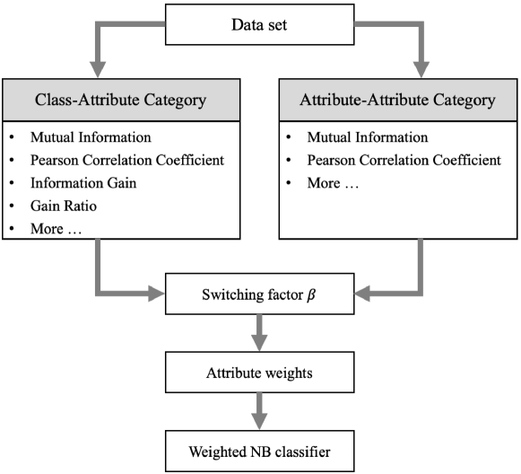
Figure 1: A general framework for adaptive two-index fusion attribute weighted NB

3.2 Index Selection

As shown in Figure 1, the ATFNB framework contains two widely used types of the attribute correlation: class-attribute and attribute-attribute. The class-attribute category is to measure the correlation between attributes and classes. The stronger the correlation between attribute and class, the more significant the attribute’s contribution to the classification. Thus, the index value is positively correlated with the weight. Common indexes in this category contain mutual information, Pearson correlation coefficient, information gain, and gain ratio, etc. The attribute-attribute category is to measure the redundancy between attributes. In order to satisfy the independence assumption of Naive Bayes as much as possible, attributes with high redundancy are assigned small weights. Thus, the weight is inversely correlated to the index value. Common measures of redundancy between attributes include mutual information and Pearson correlation coefficient, etc.

By selecting different indexes, the ATFNB framework can become any weighted NB model, including the existing weighted NB models. If only the gain ratio is selected from class-attribute category, ATFNB will degenerate into the single-index WNB model. If the class-attribute and attribute-attribute category both choose the mutual information, ATFNB will become the two-index CFW model. Thus, the index selection is a critical step in the ATFNB framework. Any two indexes are selected from the two categories can generate various models, which may achieve different results. In Section 5.3, the classification performances of different index selections are detailed discussed.

3.3 A quick algorithm for the switching factor $\beta$

Since the significantly discriminative attribute should be highly correlated with the class and has low redundancy with other attributes, its weights should be positively associated with the difference between class-attribute correlation and attribute-attribute intercorrelation[34]. The mathematics formula of the weight $w_{j}$ can be defined by Equation 11.

$$w_{j}=\underbrace{class\_attribute}_{CA_{j}}-\underbrace{attribute\_attribute}_{AA_{j}}$$ (11)

where $CA_{j}$ and $AA_{j}$ represents the values of the selected class-attribute index and attribute-attribute index, respectively. The existing two-index methods, CFW, consider that the contributions of two indexes are equivalent[34]. However, various indexes contain different characteristic, and the equivalent contribution of two indexes is unreasonable. Thus, we introduce a switching factor $\beta$ to adaptively control the ratio of two indexes. After incorporating the switching factor $\beta$, Equation 11 can be rewritten as Equation 12.

$$w_{j}=\beta\times{CA_{j}}-(1-\beta)\times{AA_{j}}$$ (12)

where the switching factor $\beta\in[0,1]$ .

Conventionally, the step-length searching strategy can be applied to search the optimal interval of $\beta$. But the accuracy and computational efficiency are effected by the step size. When the step size gets smaller, the optimal interval of $\beta$ is more accurate but get very slower. Thus, we propose a quickly algorithm to calculate the optimal interval of switching factor $\beta$. Firstly, the basic weighted NB model (Equation 4) is logarithmically transformed, and the detailed transformation process is shown as follow.

$$T(x_{i},c) =log(P(c))+\sum_{j=1}^{n}log{(P(x_{ij}|c))}^{w_{j}}$$ (13)

$$=log(P(c))+\begin{bmatrix}w_{1},...,w_{j}\end{bmatrix}\begin{bmatrix}log(P(x_{i1}|c))\\ ...\\ log(P(x_{ij}|c))\end{bmatrix}$$

$$=\beta\underbrace{\begin{bmatrix}(CA_{1}+AA_{1}),...,(CA_{j}+AA_{j})\end{bmatrix}\begin{bmatrix}log(P(x_{i1}|c))\\ ...\\ log(P(x_{ij}|c))\end{bmatrix}}_{K_{c}}$$

$$+\underbrace{log(P(c))-\begin{bmatrix}P_{1},...,P_{j}\end{bmatrix}\begin{bmatrix}log(P(x_{i1}|c))\\ ...\\ log(P(x_{ij}|c))\end{bmatrix}}_{M_{c}}$$

$$=\beta_{i}\times K_{c}+M_{c}$$

where $T(x_{i},c)$ is the probability value that the instance $x_{i}$ belonging to class c. $\beta_{i}$ is the interval when instance $x_{i}$ is correctly classified.

Based on Equation 13, a probability set $S_{i}$ can be constructed to store the probability values of instances $x_{i}$ belonging to different classes. The probability set of $x_{i}$ is $S_{i}=\{T(x_{i},c_{1}),T(x_{i},c_{2}),…,T(x_{i},c_{K})\}$. If the correct label of $x_{i}$ is $c_{k}$, $T(x_{i},c_{k})$ should be greater than the other probability values in $S_{i}$. This can be defined as follow.

$$T(x_{i},c_{k})\textgreater\{S_{i}-T(x_{i},c_{k})\}$$ (14)

When the instance $x_{i}$ is correctly classified, the interval of $\beta_{i}$ can be obtained. For $m$ instances, a set $G=\{\beta_{1},\beta_{2},…,\beta_{m}\}$ contains the $m$ interval corresponding to each instance. To calculate the optimal interval $\beta^{*}$ from G, that any value in the interval can obtain the same classification accuracy on the training set. The upper and lower bounds of all intervals in $G$ are sorted in ascending order $Q=\{value_{1},value_{2},…,value_{q}\}$. Any two adjacent values in Q are regarded as the lower and upper bounds of a subinterval. Thus, Q can generate $q-1$ subintervals. The subintervals in $R=\{\gamma_{1},\gamma_{2},...,\gamma_{q-1}\}$ satisfying Equation 15 are taken as $\beta^{*}$.

$$max\{\sum_{i=1}^{m}\tau(\gamma_{1},\beta_{i}),\sum_{i=1}^{m}\tau(\gamma_{2},\beta_{i}),...,\sum_{i=1}^{m}\tau(\gamma_{q-1},\beta_{i})\}$$ (15)

where $\tau$(·) is a binary function, which takes the value 1 if $\gamma_{q-1}$ is a subset of $\beta_{i}$ and 0 otherwise, as shown in Equation 16.

$$\tau=\left\{\begin{array}[]{cc}1,&if\gamma_{q-1}\subseteq\beta_{i}.\\ 0,&otherwise.\end{array}\right.$$ (16)

According to the above derivation processes, the Quick algorithm for the Switching Factor(QSF) is described in Algorithm 1.

Algorithm 1${\colon}$QSF

Input$\colon$class-attribute($CA_{j}$), attribute-attribute($AA_{j}$), Dataset D

For each instance $x_{i}$ in D$\colon$

For each class c in C$\colon$

Calculate $K_{c}$ and $M_{c}$ in Equation 13.

According $K_{c}$ and $M_{c}$, get $T(x_{i},c)$.

End

$S_{i}=\{T(x_{i},c_{1}),T(x_{i},c_{2}),…,T(x_{i},c_{K})\}$

If instance $x_{i}$ label is $c_{k}$$\colon$

You can find value that satisfies Equation 14, it is recorded as $\beta_{i}$,

otherwise $\beta_{i}$=$\emptyset$.

End

$G=\{\beta_{1},\beta_{2},…,\beta_{m}\}$

End

For each $\gamma_{q-1}$

Find the subinterval $\beta^{*}$ that conforms to Equation 15.

End

Output$\colon$$\beta^{*}$

Any value in $\beta^{*}$ can achieve consistent classification accuracy in dataset $D$, so we choose any value from optimal interval $\beta^{*}$. Once obtaining the value of switching factor, the weight $w_{i}$ can be calculated by Equation 12.

3.4 The Implementation of ATFNB

The general framework of ATFNB is briefly described in Algorithm 2. According to Algorithm 2, we can see that how to select two indexes $AA_{j}$ and $CA_{j}$, and how to learn the switching factor $\beta$ are two crucial problems. To select $AA_{j}$ and $CA_{j}$, several indexes are listed in Subsection 3.2. To learn the value of the switching factor $\beta$, we single out a QSF algorithm in Subsection 3.3. Once the value of the switching factor $\beta$ is obtained, we can use Equation 12 to calculate the weights of each attributes. Finally, these weights are applied to construct an attribute weighted NB classifier.
Algorithm 2${\colon}$ATFNB Framework Input$\colon$ Training set D, Test set X     (1) For each attribute $A_{j}$ in D         calculating (attribute-attribute) index $AA_{j}$         calculating (class-attribute) index $CA_{j}$.     (2) According to QSF, the value of the switching factor $\beta$ is solved.     (3) According to Equation 12, weight matrix is obtained.     (4) According to Equation 4, the class label of each instance in X is predicted. Output$\colon$Class label of instances in X

4 Experiments and Results

4.1 Experimental data

To verify the effectiveness of ATFNB, a collection of 50 benchmark datasets and 15 groups of leaf dataset are conducted.

The 50 benchmark classification datasets are chosen from the University of California at Irvin (UCI) repository[36],which represent various fields and data characteristics listed in Table LABEL:T2. We use the mean of the corresponding attribute to replace the missing data values in each dataset, then apply chi-square-based algorithm to discretize the numerical attribute values [37]. The amount of discretization of each attribute is consistent with the number of types of class labels.

Table 2: Descriptions of 50 UCI datasets used in the experiments

Dataset	Instance number	Attribute number	Class number
abalone	4177	8	3
acute	120	6	2
aggregation	788	2	7
balance-scale	625	4	3
bank	4521	16	2
banknote	1372	4	2
blood	748	4	2
breast-cancer	286	9	2
breast-tissue	106	9	6
bupa	345	6	2
car	1728	6	4
chart_Input	600	60	6
climate-simulation	540	18	2
congressional-voting	435	16	2
connectionist	208	60	2
dermatology	366	34	6
diabetes	768	8	2
ecoli	336	7	8
energy-y1	768	8	3
fertility	100	9	2
glass	214	9	6
haberman-survival	306	3	2
iris	150	4	3
jain	373	2	2
knowledge	172	5	4
libras	360	90	15
low-res-spect	531	100	9
lymphography	148	18	4
magic	19020	10	2
mammographic	961	5	2
promoters	106	57	2
splice	3190	60	3
nursery	12960	8	5
page-blocks	5473	10	5
pima	768	8	2
planning	182	12	2
post-operative	90	8	3
robotnavigation	5456	24	4
seeds	210	7	3
sonar	208	60	2
soybean	683	35	18
spect	265	22	2
synthetic-control	600	60	6
tic-tac-toe	958	9	2
titanic	2201	3	2
twonorm	7400	20	2
wall-following	5456	24	4
waveform	5000	21	3
wilt	4839	5	2
wine	178	13	3

The Flavia dataset contains 32 types of leaf and each leaf has 55-77 pieces. Four texture and ten shape features of each leaf are extracted based on the grayscale and binary images[38]. We construct 15 groups to comparative experiments, and each group randomly selects 15 kinds of leaves from the whole Flavia dataset. The detailed characteristics of 15 groups are listed in Table 3. Then the same pro-processing pipeline as the UCI dataset are applied to discretize continuous attributes.

Table 3: Descriptions of 15 groups from Flavia dataset used in the experiments

Group	Instance number	Attribute number	Class number
$G\_1$	869	14	15
$G\_2$	888	14	15
$G\_3$	865	14	15
$G\_4$	887	14	15
$G\_5$	884	14	15
$G\_6$	919	14	15
$G\_7$	892	14	15
$G\_8$	881	14	15
$G\_9$	864	14	15
$G\_10$	879	14	15
$G\_11$	895	14	15
$G\_12$	888	14	15
$G\_13$	927	14	15
$G\_14$	924	14	15
$G\_15$	904	14	15

4.2 Experimental Setting

ATFNB is a general framework of attribute weighted naive Bayes, which can adaptively fuse any two indexes. According to Figure 1, we select two simple and popular indexes from two categories: information gain from class-attribute category and Pearson correlation coefficient from attribute-attribute category. Notably, ATFNB refers to a specific NB model fused the above two indexes in the following experiments, and no longer represents a general framework.

For the class-attribute category, information gain describes the information content provided by the attribute for the classification. The formula of information gain is shown in Equation 17.

$$Gain(D;A_{j})=Ent(D)-\sum_{v=1}^{V}\frac{|D^{v}|}{|D|}Ent(D^{v})$$ (17)

where $Ent(D)$ is the information entropy. The discrete attribute $A_{j}$ has V values $\{a^{1},a^{2},…,a^{V}\}$. $D^{v}$ indicates that the $v$-$th$ branch node contains all the instances in dataset $D$, whose value is $a^{V}$ on the attribute $A_{j}$.

For the attribute-attribute category, Pearson correlation coefficient is used to calculate the correlation between attributes $A_{i}$ and $A_{j}$, and the formula can be written as Equation 18.

$$\rho(A_{i};A_{j})=|\frac{cov(A_{i},A_{j})}{\sigma_{A_{i}}\sigma_{A_{j}}}|$$ (18)

where $cov(A_{i},A_{j})$ represents the covariance between attributes $A_{i}$ and $A_{j}$, $\sigma_{A_{i}}$ and $\sigma_{A_{j}}$ represent the standard deviation of $A_{i}$ and $A_{j}$, respectively.

Once obtaining above two indexes, the weight of each attribute $A_{j}$ can be calculated as Equation 19.

$$w_{j}=\beta\times NGain(D;A_{j})-(1-\beta)\times avg\_PCC(A_{j})$$ (19)

where $NGain(D;A_{j})$ is expressed as the normalized value of attribute information gain, and $avg\_PCC(A_{j})$ represents the average degree of redundancy between the $i$-$th$ attribute and other attributes. The formula of $avg\_PCC(A_{j})$ is shown in Equation 20.

$$avg\_PCC(A_{j})=\frac{1}{n-1}\sum_{{j=1}\cap{j\neq i}}^{n}N\rho(A_{i};A_{j})$$ (20)

where $N\rho(A_{i};A_{j})$ is expressed as the normalized value between attributes $A_{i}$ and $A_{j}$.

To validate the classification performance, we compare ATFNB to standard NB and two existing state-of-the-art filter weighted methods. In addition, the original CFW is a specific model of our framework under the switching factor $\beta$=0.5. When the switching factor $\beta$ of CFW can be adaptively obtained from the dataset, the original CFW evolves into CFW-$\beta$. Now, we introduce these comparisons and their abbreviations as follows:

• NB: the standard naive Bayes model [39].

• WNB: NB with gain ratio attribute weighting [30].

• CFW: NB with MI class-specific and attribute-specific attribute weighting [34].

• CFW-$\beta$: CFW with the adaptive switching factor $\beta$.

4.3 The effectiveness of the switching factor $\beta$

The switching factor $\beta$ can be adaptively adjusted to obtain the optimal ratio for different datasets. In order to verify the effectiveness and efficiency of the switching factor $\beta$, we compare QSF algorithm with Step-Length Searching(SLS) algorithm. SLS algorithm generates $\beta$ with 0.01 as the step size. The optimal interval of switching factor $\beta$ by QSF and SLS algorithm in four datasets are shown in Figure 2.

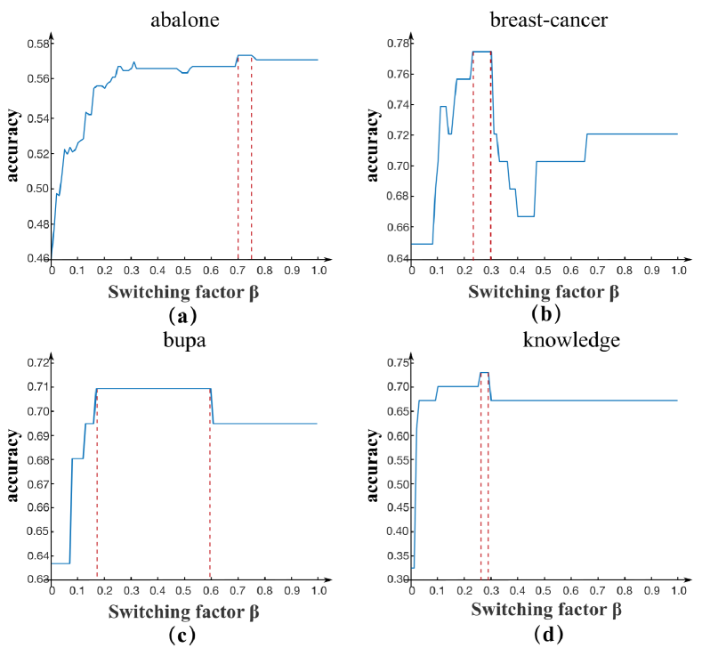
Figure 2: The optimal switching factor $\beta$ of QSF and SLS algorithms in four datasets.The blue solid line represents the accuracy of each step size by SLS, and the red dotted lines represent the optimal interval obtained by QSF

From Figure 2, either SLS or QSF algorithms, the optimal interval of $\beta$ in each dataset are biased. On abalone, the lower bound of the interval of $\beta$ is greater than 0.5. On breast-cancer and knowledge, the upper bound of the interval of $\beta$ is less than 0.5. Only the interval of $\beta$ in bupa contains 0.5. Thus, it can be concluded that the switching factor $\beta$ value set as 0.5 is unreasonable for all datasets. In addition, it can be clearly seen that the interval size of switching factor $\beta$ is inconsistent. On bupa, the interval size of $\beta$ is largest. On the contrary, the size is the smallest on knowledge.

Table 4: The optimal interval of switching factor $\beta$ and run-time by SLS and QSF

Dataset	The interval of switching factor $\beta$		Time(s)
	SLS	QSF	SLS	QSF	Speed
bupa	[0.17, 0.59]	[0.1687, 0.5937]	7.4908	0.0119	$\times$629
abalone	[0.70, 0.75]	[0.6988, 0.7521]	16.826	0.1068	$\times$157
breast-cancer	[0.23, 0.31]	[0.2257, 0.3129]	6.8023	0.0389	$\times$174
knowledge	[0.27, 0.29]	[0.2688, 0.2954]	6.1298	0.0229	$\times$267

The optimal interval of switching factor $\beta$ and run-time calculated by SLS and QSF are shown in Table 4. From Table 4, we can see that two optimal intervals obtained by SLS and QSF algorithms have a high coincidence degree. If we reduce the step size of SLS, the coincidence degree between two algorithms will further improve. Yet, SLS will become very inefficient. For QSF algorithm, the run-time is obviously faster than SLS, and speeds up 150 times at least. Therefore, QSF is not only more accurate than SLS, but also more efficient.

4.4 Experimental results on UCI Dataset

Table LABEL:T5 shows the detailed classification accuracy results of five algorithms. All classification accuracy is obtained by averaging the results of 30 independent runs. Five algorithms are performed on the same training set and testing set. We conduct a group of experiments on 50 UCI dataset to compare ATFNB with NB, WNB, CFW and CFW-$\beta$ in terms of classification accuracy.

indicates that ATFNB is significantly better than its competitors (NB, WNB, CFW) through two-tailed t-test at the $p$=0.05 significance level [40]. At the bottom of the table, G represents the number of data sets with the highest classification accuracy among the four algorithms (ATFNB, WNB, CFW, NB). W represents the classification accuracy is higher than ATFNB for the number of datasets, L means the opposite of W.

Table 5: Classification accuracy comparisons for ATFNB versus NB, WNB, CFW, CFW-$\beta$ on UCI dataset

Dataset	NB	WNB	CFW	ATFNB	CFW-$\beta$
abalone	0.5886	0.5871 *	0.5890 *	0.5908	0.5926
acute	0.9958	0.9521 *	0.9948	0.9635	0.9813
aggregation	0.9890	0.9882	0.9761 *	0.9875	0.9824
balance-scale	0.8592 *	0.8728	0.8312 *	0.8984	0.8581
bank	0.8765	0.8831	0.8901	0.8822	0.9076
banknote	0.8636	0.8468	0.8491	0.8498	0.8338
blood	0.7597 *	0.7733	0.7720 *	0.7847	0.7990
breast-cancer	0.7214 *	0.7059 *	0.7331	0.7472	0.7422
breast-tissue	0.5727	0.5955	0.5818 *	0.6091	0.6158
bupa	0.6232	0.5942 *	0.6174 *	0.6333	0.6299
car	0.8523	0.6965 *	0.7671 *	0.8014	0.8101
chart_Input	0.9533	0.9367	0.9558	0.9455	0.9488
climate-simulation	0.9137	0.9178	0.9174	0.9181	0.9209
congressional-voting	0.6149 *	0.6345 *	0.6253 *	0.6506	0.6614
connectionist	0.7238 *	0.7429 *	0.7214 *	0.7667	0.7560
dermatology	0.9797	0.9644	0.9757	0.9649	0.9665
diabetes	0.7377	0.6584 *	0.7403	0.7422	0.7611
Ecoli	0.8135	0.7706 *	0.7588 *	0.8245	0.7981
energy-y1	0.8874	0.8225 *	0.8701	0.8463	0.8813
fertility	0.8400 *	0.8500	0.8350 *	0.8650	0.8669
glass	0.7023	0.6837 *	0.6930	0.7193	0.7233
haberman-survival	0.7532 *	0.7468 *	0.7403 *	0.7710	0.7791
Iris	0.9133	0.9100 *	0.9167	0.9367	0.9099
Jain	0.9464	0.9368	0.9379	0.9397	0.9399
knowledge	0.7371*	0.7743 *	0.7629 *	0.8057	0.7989
libras	0.5903	0.5917	0.5847	0.5965	0.6122
low-res-spect	0.8037 *	0.8018 *	0.8131*	0.8318	0.8411
lymphography	0.8122 *	0.7889 *	0.8233	0.8334	0.8399
magic	0.7300	0.6885 *	0.7411	0.7674	0.7782
mammographic	0.8290 *	0.8394	0.8446	0.8549	0.8679
promoters	0.9091 *	0.9045 *	0.9242 *	0.9545	0.9302
splice	0.9475	0.9376 *	0.9580	0.9414	0.9677
nursery	0.9043	0.8089 *	0.8812	0.8961	0.9002
page-blocks	0.9300 *	0.9404	0.9545 *	0.9684	0.9690
pima	0.7338 *	0.6688 *	0.7330 *	0.7599	0.7613
planning	0.6000 *	0.7189	0.6919 *	0.7378	0.7500
post-operative	0.7222 *	0.8519 *	0.7593 *	0.9074	0.8489
robotnavigation	0.8760 *	0.9159	0.9095	0.9179	0.9199
seeds	0.8747	0.8622	0.8762	0.8655	0.8881
sonar	0.7625	0.7429 *	0.7571 *	0.7734	0.7662
soybean	0.9036	0.8730	0.9117	0.8781	0.9049
spect	0.6566 *	0.6604 *	0.6792 *	0.7151	0.7288
synthetic-control	0.9677	0.9458	0.9698	0.9567	0.9675
tic-tac-toe	0.7141	0.6589 *	0.7109	0.7005	0.7201
titanic	0.7782	0.6680 *	0.7751	0.7822	0.7991
twonorm	0.9384	0.9364	0.9388	0.9489	0.9346
wall-following	0.8032	0.7964	0.8137	0.7976	0.8199
waveform	0.8080 *	0.7960 *	0.8172 *	0.8355	0.8317
wilt	0.9472	0.9374 *	0.9475	0.9523	0.9538
wine	0.9694	0.9625	0.9750	0.9697	0.9622
Average	0.8146	0.8028	0.8169	0.8317	0.8345
G/W/L	9/15/35	0/2/48	8/12/38	33 / /

Compared with WNB, CFW, NB, the accuracy of ATFNB on 33 datasets is the highest, which far exceeds WNB (0 datasets), CFW (8 datasets), NB (9 datasets). The average accuracy of ATFNB is 83.17%, which is significantly higher than those of algorithms, and the improvement of average accuracy is approximately 3%, 2%, and 2%, respectively.

In addition, the average accuracy of CFW-$\beta$ increases by 1.76% compared with CFW. This means that the adaptive switching factor can improve the existing two-index NB model. Compared with ATFNB, the average accuracy of CFW-$\beta$ is higher than ATFNB. The reason is that mutual information (class-attribute) and mutual information (attribute-attribute) are included in CFW-$\beta$, which has a more powerful representation than information gain and Pearson correlation coefficient in ATFNB. In Subsection 5.3, models generated by different combinations of indexes are discussed in detail.

Base on the accuracy result, we use a two-tailed t-test at the $p=0.05$ to compare each pair of algorithms beside CFW-$\beta$. Table 6 summarizes the comparison results on UCI Dataset. From Table 6, ATFNB has significant advantages over other weighting algorithms. ATFNB is better than WNB(28 wins and zero loss), CFW(22 wins and 4 loss), and NB(19 wins and 5 loss).

Table 6: Summary two-tailed t-test results of classification accuracy with regard to ATFNB on UCI dataset

Algorithm	ATFNB	WNB	CFW	NB
ATFNB	—	2(0)	12(4)	15(5)
WNB	48(28)	—	35(16)	34(19)
CFW	38(22)	15(5)	—	20(8)
NB	35(19)	16(9)	30(11)	—

For each i(j), $i$ represents the number of datasets with higher classification accuracy obtained by the column algorithm than the row algorithm, and $j$ represents the number of datasets in which the column algorithm has a significant advantage over the row algorithm.

Based on the classification accuracy of Table LABEL:T5, we utilize the Wilcoxon signed-rank test to compare four algorithms. Wilcoxon signed-rank test is a non-parametric statistical test, which ranks the performance differences of the two algorithms for each dataset, considering both the sign of the difference and the order of the difference. Tables 7 shows the ranks calculated by the Wilcoxon test. In Table 7, the numbers above the diagonal line indicate the sum of ranks for the datasets of the algorithm in the row that is better than the algorithm in the corresponding column (The sum of the ranks for the positive difference, represented by R+). Each number below the diagonal is the sum of ranks for the datasets in which the algorithm in the column is worse than the algorithm in the corresponding row (The sum of the ranks for the negative difference, represented by R-). According to the critical value table of the Wilcoxon test, for Table 7, when $\alpha$=0.05 and n=50, if the smaller of R+ and R- is equal to or less than 434, we consider that two classifiers are significantly different, so we reject the null hypothesis.

Table 7: Ranks of the Wilcoxon test with regard to ATFNB on UCI dataset

Algorithm	ATFNB	WNB	CFW	NB
ATFNB	—	1268	1007.5	961.5
WNB	7	—	308.5	391.5
CFW	267.5	966.5	—	771
NB	313.5	883.5	504	—

Table 8: Summary of the Wilcoxon test with regard to ATFNB on UCI dataset

Algorithm	ATFNB	WNB	CFW	NB
ATFNB	—	$\circ$	$\circ$	$\circ$
WNB	$\bullet$	—	$\circ$	$\circ$
CFW	$\bullet$	$\bullet$	—
NB	$\bullet$	$\bullet$		—

$\bullet$  indicates that the algorithm in the column is improved compared to the algorithm in the corresponding row.
$\circ$  indicates that the algorithm in the row is better than the algorithm in the corresponding column.

According to the results of the Wilcoxon signed rank-sum test, on the UCI dataset, ATFNB is significantly better than WNB ($R^{+}=1268,R^{-}=7$), CFW ($R^{+}=1007.5,R^{-}=267.5$) and Standard NB ($R^{+}=961.5,R^{-}=313.5$).

4.5 Experimental results on Flavia Dataset

In order to further verify the effectiveness of ATFNB, we conduct 15 groups of experiments on Flavia dataset. We randomly divide the data in each group of experiments 30 times and use a two-tailed t-test for the results of 30 experiments. The detailed results are shown in Table 9.

Table 9: Classification accuracy comparisons for ATFNB, NB, WNB, CFW, CFW-$\beta$ on Flavia dataset.

Group	NB	WNB	CFW	ATFNB	CFW-$\beta$
G_1	0.8253 *	0.8506 *	0.8552 *	0.8805	0.9011
G_2	0.8337	0.8629	0.8742	0.8444	0.8668
G_3	0.7874 *	0.8484	0.8312	0.8786	0.8771
G_4	0.8562 *	0.8854 *	0.8899	0.8987	0.9022
G_5	0.8016 *	0.8129	0.8050 *	0.8174	0.8177
G_6	0.8822	0.8729 *	0.8903	0.8843	0.8801
G_7	0.9134 *	0.9137 *	0.9322	0.9233	0.9400
G_8	0.9011	0.8812 *	0.8927	0.8904	0.9022
G_9	0.9122	0.9100	0.9033 *	0.9422	0.8891
G_10	0.8135 *	0.8213 *	0.8200 *	0.8422	0.8399
G_11	0.8572	0.8734	0.8534	0.8799	0.8912
G_12	0.8356	0.8132 *	0.8224	0.8233	0.8335
G_13	0.7724 *	0.7787 *	0.7732 *	0.7987	0.7887
G_14	0.8342 *	0.8344	0.8322 *	0.8458	0.8422
G_15	0.9169 *	0.9224 *	0.9243 *	0.9321	0.9095
Average	0.8495	0.8588	0.8600	0.8721	0.8720
G/W/L	2/2/13	0/1/14	3/4/11	10 / /

Comparing ATFNB with other existing classifiers (WNB, CFW, NB), the average accuracy of ATFNB is 87.21%, which is significantly higher than those of algorithms, and the improvement of average accuracy is approximately 3%, 1.5%, 1%, respectively. In 15 groups of experiments, ATFNB achieved the highest classification accuracy among 10 groups of data, which is far better than NB, WNB, and CFW.

The average accuracy of CFW-$\beta$ is slightly lower than ATFNB, but the average accuracy of CFW-$\beta$ is higher than CFW. On Flavia, the choice of indexes has little effect on the average accuracy, but adding a switching factor $\beta$ to the model can effectively improve the performance of model.

We Summarize the results of the two-tailed test in Table 9, as shown in Table 10. In Table 10, ATFNB is better than WNB(9 wins and zero loss), CFW(7 wins and 1 loss), and NB(9 wins and zero loss).

Table 10: Summary two-tailed t-test results of classification accuracy with regard to ATFNB on Flavia dataset

Algorithm	ATFNB	WNB	CFW	NB
ATFNB	—	1(0)	4(1)	2(0)
WNB	14(9)	—	8(3)	4(1)
CFW	11(7)	7(4)	—	5(1)
NB	13(9)	11(6)	10(5)	—

On the basis of Table 9, we use the Wilcoxon signed-rank test to compare four algorithms. According to the critical value table of the Wilcoxon test, for Table 11, when $\alpha$=0.05 and n=15, if the smaller of R+ and R- is equal to or less than 25, we consider that two classifiers are significantly different, so we reject the null hypothesis.

Table 11: Ranks of the Wilcoxon test with regard to ATFNB on Flavia dataset

Algorithm	ATFNB	WNB	CFW	NB
ATFNB	—	110	96	110.5
WNB	10	—	52	89
CFW	24	68	—	87
NB	9.5	31	33	—

Table 12: Summary of the Wilcoxon test with regard to ATFNB on Flavia dataset

Algorithm	ATFNB	WNB	CFW	NB
ATFNB	—	$\circ$	$\circ$	$\circ$
WNB	$\bullet$	—
CFW	$\bullet$		—
NB	$\bullet$			—

In the Flavia dataset, the ATFNB algorithm is compared with WNB ($R^{+}=110,R^{-}=10$), CFW ($R^{+}=96,R^{-}=24$) and standard NB ($R^{+}=110.5,R^{-}=9.5$) has obvious advantages.

5 Discussion

5.1 The influence of instance and attribute number

To further analyze the relationship between the performance of ATFNB and the characteristic of dataset, we observe their performance from two perspectives of instances number and attributes number. In terms of the number of instances, we divide the dataset into two categories: less than 500 instances and greater than or equal to 500 instances. Similar, according to the number of attributes, we divide attributes into two categories: the number of attributes is less than 15, and the number of attributes is greater than or equal to 15. Then, we combine above two criteria and result in four divisions. Finally, we calculate the percentage of the dataset with the highest classification accuracy of ATFNB and competitors (NB, WNB, CFW) in eight divisions. The detailed results are shown in Table 13.

Table 13: ATFNB and competitors obtain the percentage of the dataset with the highest classification accuracy in each division

Data Characteristics		Number	ATFNB (%)	Competitors (%)
Instance number	<500	23	78.26	21.74
	$\geq$500	27	56.25	43.75
Attribute number	<15	31	67.74	32.26
	$\geq$15	19	63.16	36.84
Instance&Attribute	<500&<15	15	73.33	26.67
	<500&$\geq$15	8	87.50	12.50
	$\geq$500&<15	16	62.50	37.50
	$\geq$500&$\geq$15	11	45.45	54.55

From Table 13, we can clearly find in which circumstance ATFNB performs better than the competitors. Here, we summarize the highlights as follow:
(1) On the datasets with the number of instances less than 500, the percentage of the dataset with the highest classification accuracy of ATFNB (78.26%) is higher than the number of instances is greater than or equal to 500 (56.25%).
(2) For datasets with attributes less than 15, the percentage of datasets with the highest classification accuracy of ATFNB (67.74%) is also higher than that with attributes greater than or equal to 15 (63.16%).
(3) When the number of instances is less than 500, and the number of attributes is greater than 15, the percentage of the dataset with the highest classification accuracy of ATFNB (87.5%) is significantly higher than that of the other three types of datasets (73.33%, 62.50%, 45.45%).

The performance of ATFNB has obvious advantages on the datasets whose instance number is smaller than 500, especially attribute number is greater than or equal to 15, such as the dataset “congressional-voting”. By contrast, ATFNB does not perform well on datasets with large instances and attributes. In a word, ATFNB can be perfectly suitable for small data classification, and is not limited by dimensions.

5.2 The distribution of the switching factor $\beta$

In Section 4.3, we have validated the effectiveness of the switching factor $\beta$ in ATFNB. Here, the distributions of the switching factor $\beta$ in various datasets are further analyzed. We firstly list the interval of the switching factor $\beta$ on 50 UCI datasets as shown in Table 14. From Table 14, we can summarize that the lower bound of the optimal interval in 11 datasets is greater than 0.5, the upper bound of the optimal interval in 23 datasets is less than 0.5, and the optimal interval of the rest 16 datasets contains 0.5. In ATFNB, the information gain and Pearson correlation coefficient provide different contributions on the 50 UCI datasets. In addition, these results further demonstrates that the switching factor $\beta$ set as a fixed value is unreasonable.

Table 14: The interval of switching factor $\beta$ on 50 UCI Datasets

Dataset	Interval ($\beta$)	Mark	Dataset	Interval ($\beta$)	Mark
abalone	[0.7122, 0.8311]	$\bigcirc$	libras	[0.5377, 0.8832]	$\bigcirc$
acute	[0.4418, 0.9433]	$\bigtriangleup$	low-res-spect	[0.6552, 0.7211]	$\bigcirc$
aggregation	[0.5529, 0.8832]	$\bigtriangleup$	lymphography	[0.3344, 0.4834]	$\square$
balance-scale	[0.3233, 0.4537]	$\square$	magic	[0.6733, 0.8122]	$\bigcirc$
bank	[0.4198, 0.7691]	$\bigtriangleup$	mammographic	[0.1229, 0.3879]	$\square$
banknote	[0.3144, 0.3914]	$\square$	promoters	[0.4876, 0.8867]	$\bigtriangleup$
blood	[0.2243, 0.5532]	$\bigtriangleup$	splice	[0.0512, 0.1321]	$\square$
breast-cancer	[0.2311, 0.3521]	$\square$	nursery	[0.5211, 0.5908]	$\bigcirc$
breast-tissue	[0.3566, 0.4513]	$\square$	page-blocks	[0.6322, 0.7109]	$\bigcirc$
bupa	[0.1533, 0.6588]	$\bigtriangleup$	pima	[0.1566, 0.3118]	$\square$
car	[0.3211, 0.3987]	$\square$	planning	[0.1829, 0.4721]	$\square$
chart_Input	[0.4592, 0.8311]	$\bigtriangleup$	post-operative	[0.0187, 0.2100]	$\square$
climate-simulation	[0.2301, 0.3255]	$\square$	robotnavigation	[0.7122, 0.7830]	$\bigcirc$
congressional-voting	[0.2199, 0.3472]	$\square$	seeds	[0.4288, 0.8543]	$\bigtriangleup$
connectionist	[0.0912, 0.1388]	$\square$	sonar	[0.0521, 0.1487]	$\square$
dermatology	[0.3365, 0.8987]	$\bigtriangleup$	soybean	[0.2759, 0.3108]	$\square$
diabetes	[0.2355, 0.5243]	$\bigtriangleup$	spect	[0.1802, 0.2499]	$\square$
Ecoli	[0.7360, 0.9211]	$\bigcirc$	synthetic-control	[0.2480, 0.4033]	$\square$
energy-y1	[0.3211, 0.9219]	$\bigtriangleup$	tic-tac-toe	[0.1213, 0.1870]	$\square$
fertility	[0.0511, 0.4390]	$\square$	titanic	[0.4697, 0.6122]	$\bigtriangleup$
glass	[0.1229, 0.1833]	$\square$	twonorm	[0.5833, 0.6291]	$\bigcirc$
haberman-survival	[0.2166, 0.6345]	$\bigtriangleup$	wall-following	[0.4128, 0.4736]	$\square$
iris	[0.3522, 0.8799]	$\bigtriangleup$	waveform	[0.7398, 0.7933]	$\bigcirc$
jain	[0.3409, 0.8577]	$\bigtriangleup$	wilt	[0.6103, 0.6899]	$\bigcirc$
knowledge	[0.3012, 0.4522]	$\square$	wine	[0.3881, 0.9220]	$\bigtriangleup$

$\bigcirc$  indicates that the lower bound value of $\beta$ interval is greater than 0.5.
$\square$  indicates that the upper bound value of $\beta$ interval is less than 0.5.
$\bigtriangleup$  indicates 0.5 is in the interval.

Table 15: The relationship between the switching factor $\beta$ in the ATFNB and the characteristics of the dataset

Data Characteristics		Number	$\bigcirc$ (%)	$\bigtriangleup$ (%)	$\square$ (%)
Instance number	<500	23	8.70	39.13	52.17
	$\geq$500	27	33.33	25.93	40.74
Attribute number	<15	31	19.35	38.71	41.94
	$\geq$15	19	26.32	21.05	52.63
Instance&Attribute	<500&<15	15	6.66	46.67	46.67
	<500&$\geq$15	8	12.50	25.00	62.50
	$\geq$500&<15	16	31.25	31.25	37.50
	$\geq$500&$\geq$15	11	36.36	18.18	45.46

To further investigate the relationship between the distribution of switching factor $\beta$ and the characteristics of dataset, we apply the same division criteria as Section 5.1 on 50 UCI datasets and summarize detailed results in Table 15. From Table 15, we can observe the preference between the data characteristic and the distribution of the switching factor $\beta$, and summarize the highlights as follows:
(1) If the number of instance is less than 500, the upper bound value of $\beta$ in 52.17% of the datasets is less than 0.5. The number of datasets is more than 500, and the upper bound value of $\beta$ in 40.74% of the datasets is less than 0.5.
(2) From the perspective of the number of attributes, regardless of the number of attributes, the upper bound value of $\beta$ is less than 0.5 in most datasets.
(3) Considering the number of instance and attributes simultaneously, the upper bound value of $\beta$ in 62.50% of the datasets with instances less than 500 and attributes greater than 15 is less than 0.5. On the dataset with instances greater than 500 and attribute number greater than 15, the upper bound value of $\beta$ in 45.46% of the datasets is less than 0.5.

Based on the results in Table 15, the upper bound value of $\beta$ is less than 0.5 in most datasets. We can conclude that ATFNB pays attention to Pearson correlation coefficient between attributes, especially in small instances and high-dimensional datasets.

5.3 The impact of different index combinations

The ATFNB framework contains two categories, and each category provides several popular indexes to represent the characteristic of datasets. Now, in order to analyze the impact of different index combinations, we select two any indexes from two categories respectively. Excluding the gain ratio from class-attribute category, six weighted NB models can be constructed as shown in Figure 3. Notably, ATFNB-IP and ATFNB-MM are equal to ATFNB and CFW-$\beta$ respectively.

Figure 3: The index selection of each combination

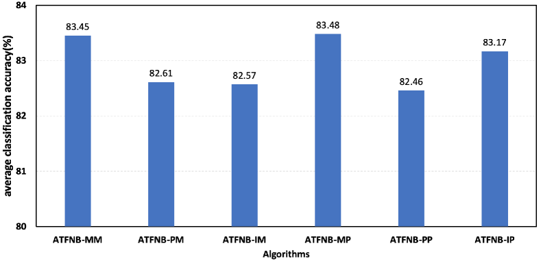
Figure 4: Average accuracy of six combinations

Then, we compare six combinations on the 50 UCI datasets, and the average accuracy of six combinations are shown in Figure 4. From Figure 4, it can be seen that ATFNB-PP receives the lowest, but average accuracy of ATFNB-PP outperforms the basic NB and NB(0.8146), WNB(0.8028) and CFW(0.8169). This further demonstrates the effectiveness of ATFNB framework with adaptive switching factor. In addition, compare with three indexed from class-attribute category, the average accuracy of ATFNB-M*(denotates ATFNB-MP and ATFNB-MM) is better than ATFNB-P* and ATFNB-I*. This means mutual information from class-attribute category is more signification than Pearson correlation coefficient and Information gain.

6 Conclusions and future work

In this paper, we propose a general framework for adaptive Two-index Fusion attribute weighted NB(ATFNB) to overcome the problems of the existing weighted methods, such as the poor representation ability with single index and the fusion problem of two indexes. ATFNB can select any one index from attribute-attribute category and class-attribute category, respectively. Then, switching factor $\beta$ is introduced to fuse two indexes and inferred by a quick algorithm. Finally, the weight of each attribute is calculated using the optimal value $\beta$ and integrated into NB classifier to improve the accuracy. The experimental results on 50 benchmark datasets and a Flavia dataset show that ATFNB outperforms the basic NB and state-of-the-art filter weighted NB models. In addition, we incorporate the switching factor $\beta$ into CFW. The results demonstrate the improved model CFW-$\beta$ significantly increase accuracy compared to CFW without the adaptive switching factor $\beta$.

In the future work, there are two direction to further improve NB model. Firstly, ATFNB maybe consider more than two indexes from different data description categories. Secondly, we hope design more new indexes to represent the correlation between class-attribute or attribute-attribute.

References

- [1] H. Zhang, L. Jiang, L. Yu, Class-specific attribute value weighting for naive bayes, Information Sciences 508 (2020) 260–274. doi:10.1016/j.ins.2019.08.071.
- [2] M. Koivisto, K. Sood, Exact bayesian structure discovery in bayesian networks, The Journal of Machine Learning Research 5 (2004) 549–573.
- [3] N. Friedman, D. Koller, Being bayesian about network structure. a bayesian approach to structure discovery in bayesian networks, Machine learning 50 (2003) 95–125. doi:10.1023/A:1020249912095.
- [4] N. Friedman, D. Geiger, M. Goldszmidt, Bayesian network classifiers, Machine learning 29 (1997) 131–163. doi:10.1023/A:1007465528199.
- [5] L. Jiang, H. Zhang, Z. Cai, A novel bayes model: Hidden naive bayes, IEEE Transactions on knowledge and data engineering 21 (2008) 1361–1371. doi:10.1109/TKDE.2008.234.
- [6] L. Jiang, S. Wang, C. Li, L. Zhang, Structure extended multinomial naive bayes, Information Sciences 329 (2016) 346–356. doi:10.1016/j.ins.2015.09.037.
- [7] D. M. Diab, K. M. El Hindi, Using differential evolution for fine tuning naïve bayesian classifiers and its application for text classification, Applied Soft Computing 54 (2017) 183–199. doi:10.1016/j.asoc.2016.12.043.
- [8] K. El Hindi, Fine tuning the naïve bayesian learning algorithm, AI Communications 27 (2014) 133–141. doi:10.3233/AIC-130588.
- [9] D. Ryu, J.-I. Jang, J. Baik, A hybrid instance selection using nearest-neighbor for cross-project defect prediction, Journal of Computer Science and Technology 30 (2015) 969–980. doi:10.1007/s11390-015-1575-5.
- [10] Z. Xie, W. Hsu, Z. Liu, M. L. Lee, Snnb: A selective neighborhood based naive bayes for lazy learning, in: Pacific-Asia Conference on Knowledge Discovery and Data Mining, Springer, 2002, pp. 104–114.
- [11] H. Zhang, L. Jiang, L. Yu, Attribute and instance weighted naive bayes, Pattern Recognition 111 (2021) 107674. doi:10.1016/j.patcog.2020.107674.
- [12] C. Elkan, et al., Boosting and naive bayesian learning, in: Proceedings of the international conference on knowledge discovery and data mining, 1997.
- [13] L. Jiang, Z. Cai, D. Wang, Improving naive bayes for classification, International Journal of Computers and Applications 32 (2010) 328–332.
- [14] J. Chen, H. Huang, S. Tian, Y. Qu, Feature selection for text classification with naïve bayes, Expert Systems with Applications 36 (2009) 5432–5435. doi:10.1016/j.eswa.2008.06.054.
- [15] D. K. Choubey, S. Paul, S. Kumar, S. Kumar, Classification of pima indian diabetes dataset using naive bayes with genetic algorithm as an attribute selection, in: Communication and computing systems: proceedings of the international conference on communication and computing system (ICCCS 2016), 2017, pp. 451–455.
- [16] M. A. Hall, G. Holmes, Benchmarking attribute selection techniques for discrete class data mining, IEEE Transactions on Knowledge and Data engineering 15 (2003) 1437–1447. doi:10.1109/TKDE.2003.1245283.
- [17] L. Jiang, Z. Cai, H. Zhang, D. Wang, Not so greedy: randomly selected naive bayes, Expert Systems with Applications 39 (2012) 11022–11028. doi:10.1016/j.eswa.2012.03.022.
- [18] C. Lee, G. G. Lee, Information gain and divergence-based feature selection for machine learning-based text categorization, Information processing & management 42 (2006) 155–165. doi:10.1016/j.ipm.2004.08.006.
- [19] X. Deng, Y. Li, J. Weng, J. Zhang, Feature selection for text classification: A review., Multimedia Tools & Applications 78 (2019) 3797–3816.
- [20] C.-H. Lee, An information-theoretic filter approach for value weighted classification learning in naive bayes, Data & Knowledge Engineering 113 (2018) 116–128. doi:10.1016/j.datak.2017.11.002.
- [21] L. Yu, L. Jiang, D. Wang, L. Zhang, Toward naive bayes with attribute value weighting, Neural Computing and Applications 31 (2019) 5699–5713. doi:10.1007/s00521-018-3393-5.
- [22] L. Jiang, L. Zhang, L. Yu, D. Wang, Class-specific attribute weighted naive bayes, Pattern recognition 88 (2019) 321–330. doi:10.1016/j.patcog.2018.11.032.
- [23] J. Wu, S. Pan, X. Zhu, Z. Cai, P. Zhang, C. Zhang, Self-adaptive attribute weighting for naive bayes classification, Expert Systems with Applications 42 (2015) 1487–1502. doi:10.1016/j.eswa.2014.09.019.
- [24] M. Hall, A decision tree-based attribute weighting filter for naive bayes, in: International conference on innovative techniques and applications of artificial intelligence, Springer, 2006, pp. 59–70.
- [25] S. Taheri, J. Yearwood, M. Mammadov, S. Seifollahi, Attribute weighted naive bayes classifier using a local optimization, Neural Computing and Applications 24 (2014) 995–1002. doi:10.1007/s00521-012-1329-z.
- [26] L. Jiang, C. Li, S. Wang, L. Zhang, Deep feature weighting for naive bayes and its application to text classification, Engineering Applications of Artificial Intelligence 52 (2016) 26–39. doi:10.1016/j.engappai.2016.02.002.
- [27] L. Zhang, L. Jiang, C. Li, G. Kong, Two feature weighting approaches for naive bayes text classifiers, Knowledge-Based Systems 100 (2016) 137–144. doi:10.1016/j.knosys.2016.02.017.
- [28] J. Wu, Z. Cai, Attribute weighting via differential evolution algorithm for attribute weighted naive bayes (wnb), Journal of Computational Information Systems 7 (2011) 1672–1679.
- [29] J. Ferreira, D. Denison, D. Hand, Weighted naive bayes modelling for data mining (2001).
- [30] H. Zhang, S. Sheng, Learning weighted naive bayes with accurate ranking, in: Fourth IEEE International Conference on Data Mining (ICDM’04), IEEE, 2004, pp. 567–570.
- [31] J. Quinlan, C4. 5: Program for machine learning morgan kaufmann, San Mateo, CA, USA (1993).
- [32] C.-H. Lee, F. Gutierrez, D. Dou, Calculating feature weights in naive bayes with kullback-leibler measure, in: 2011 IEEE 11th International Conference on data mining, IEEE, 2011, pp. 1146–1151.
- [33] S. Kullback, R. A. Leibler, On information and sufficiency, The annals of mathematical statistics 22 (1951) 79–86.
- [34] L. Jiang, L. Zhang, C. Li, J. Wu, A correlation-based feature weighting filter for naive bayes, IEEE transactions on knowledge and data engineering 31 (2018) 201–213.
- [35] M. A. Hall, Correlation-based feature selection of discrete and numeric class machine learning (2000).
- [36] A. Asuncion, D. Newman, Uci machine learning repository (2007).
- [37] R. Kerber, Chimerge: Discretization of numeric attributes, in: Proceedings of the tenth national conference on Artificial intelligence, 1992, pp. 123–128.
- [38] S. Sachar, A. Kumar, Survey of feature extraction and classification techniques to identify plant through leaves, Expert Systems with Applications 167 (2021) 114181. doi:10.1016/j.eswa.2020.114181.
- [39] P. Langley, W. Iba, K. Thompson, et al., An analysis of bayesian classifiers, in: Aaai, Vol. 90, Citeseer, 1992, pp. 223–228.
- [40] C. Nadeau, Y. Bengio, Inference for the generalization error, Machine learning 52 (2003) 239–281. doi:10.1023/A:1024068626366.