XAutoML: A Visual Analytics Tool for Understanding and Validating Automated Machine Learning
Abstract.
In the last 10 years, various automated machine learning (AutoML) systems have been proposed to build end-to-end machine learning (ML) pipelines with minimal human interaction. Even though such automatically synthesized ML pipelines are able to achieve competitive performance, recent studies have shown that users do not trust models constructed by AutoML due to missing transparency of AutoML systems and missing explanations for the constructed ML pipelines. In a requirements analysis study with 36 domain experts, data scientists, and AutoML researchers from different professions with vastly different expertise in ML, we collect detailed informational needs for AutoML. We propose XAutoML, an interactive visual analytics tool for explaining arbitrary AutoML optimization procedures and ML pipelines constructed by AutoML. XAutoML combines interactive visualizations with established techniques from explainable artificial intelligence (XAI) to make the complete AutoML procedure transparent and explainable. By integrating XAutoML with JupyterLab, experienced users can extend the visual analytics with ad-hoc visualizations based on information extracted from XAutoML. We validate our approach in a user study with the same diverse user group from the requirements analysis. All participants were able to extract useful information from XAutoML, leading to a significantly increased understanding of ML pipelines produced by AutoML and the AutoML optimization itself.
1. Introduction
ML has become a vital part in many aspects of daily life. Yet, building well-performing ML applications is a challenging and time-consuming task that requires highly specialised data scientists and domain experts. The limited availability of data scientists slows down the further dissemination of ML. \AcAutoML aims at improving the current approach of building ML applications in two aspects: (1) MLexperts can benefit from automating tedious tasks, including hyperparameter optimization (HPO), leading to higher efficiency and greater focus on more challenging tasks; and (2) domain experts can be enabled to build ML pipelines on their own without having to rely on an ML expert. In the beginning, AutoML was only used for a few aspects of the data science endeavour, e.g., tuning the hyperparameters of a classification algorithm. More recently, huge improvements have been made that enable users to automate the complete process from data encoding, preprocessing, and feature engineering to model building. Lately, researchers have proposed many new approaches for AutoML, which have reached astonishing performances, e.g., (Feurer et al., 2015; Olson and Moore, 2016; Falkner et al., 2018; Akiba et al., 2019). With the ever-increasing degree of automation, understanding and validating the behaviour of AutoML systems becomes inherently more difficult. Although multiple commercial solutions have been released in the past years, e.g., (Clouder, 2018; H2O.ai, 2019; Das et al., 2020), AutoML is still primarily an active research topic and only has a niche existence in the larger ML universe (Google LLC, 2022).
Currently, AutoML is only seen as a tool to aid human users during their ML endeavour in an interactive fashion (Wang et al., 2019b). However, current implementations are not designed with human interaction in mind. From a user’s perspective, AutoML systems are a black-box that creates another black-box, namely the ML pipeline, promising to solve their prediction problem. They behave in a take-it-or-leave-it manner without providing users sufficient information about the optimization procedure or the resulting ML pipelines. Without sufficient information, users cannot make an informed and accountable decision about whether an ML pipeline created via AutoML should be used at all. During their optimization procedure, a multitude of ML pipeline candidates are generated that are all able to solve the given task. However, AutoML systems tend to create extremely diverse candidates with no significant performance differences (Zöller and Huber, 2021). Validating and selecting a model from the abundance of provided solutions is a time-consuming task, even for seasoned ML practitioners. For domain experts, also called subject-matter experts, with specialized knowledge of a particular area but no expertise in ML, this task is practically impossible. Furthermore, modern AutoML systems build long and arbitrarily complex ML pipelines by selecting from dozens of ML primitives—each tunable by multiple hyperparameters—, making it inherently impossible for humans to grasp the complete, high-dimensional search space. In combination with the black-box nature of many AutoML systems, it is nearly impossible to understand what is going on during the optimization procedure. This lack of transparency and explainability severely limits the trust in AutoML (Li et al., 2017; Drozdal et al., 2020; Wang et al., 2021a; Crisan and Fiore-Gartland, 2021). Furthermore, this makes the application of AutoML for automated decision making in high-risk domains, like healthcare or finance, impossible.
In this article, we propose a new visual analytics tool titled eXplainable Automated Machine Learning (XAutoML) for analysing and understanding ML pipelines produced by AutoML systems. This visualization aims to empower all user groups of AutoML, namely domain experts, data scientists, and AutoML researchers, by (1) making the internal optimization procedure and search space of AutoML systems transparent and (2) providing enough information to validate and select automatically synthesized ML models quickly. By combining existing techniques from explainable artificial intelligence (XAI) and visualizations tailored to AutoML, XAutoML provides a holistic visualization that makes the performed optimizations transparent and the synthesized ML models explainable. Users can compare pipeline candidates, analyse the optimization procedure independent of the actually used AutoML system to gain process insights, inspect single ML models to gain data and model insights, and inspect ML ensembles, which are often produced during the AutoML optimization. XAutoML is integrated with JupyterLab (Project Jupyter, 2018) to blend with the usual data science workflow. It provides measures to import the result of an AutoML optimization and export analytical results directly to Jupyter for further manual analysis.
The contributions of our work are summarised as follows:
-
•
By combining existing visualization techniques with methods from XAI, XAutoML can visualize different aspects of the underlying AutoML system as well as the generated ML models in a single holistic framework covering data, model, and process insights all at once.
-
•
In semi-structured interviews, the informational needs of 36 domain experts, data scientists, and AutoML researchers for interacting with AutoML are gathered. This is the first structured evaluation of requirements of domain experts and AutoML researchers for AutoML systems at all.
-
•
We introduce two new visualizations to explain aspects of the AutoML optimization procedures for users with minimal AutoML knowledge. In combination with improved existing visualizations, XAutoML is able to visualize all important aspects of the optimization procedure of state-of-the-art AutoML systems.
-
•
We perform a user study with the same diverse user group from the requirements analysis to validate XAutoML. The study proves that XAutoML is usable and useful for participants from the three different user groups and helps validating and understanding the ML models created by AutoML. Participants highlighted the benefits of integrating the visual analytics with JupyterLab.
This article is structured as follows: Section 2 introduces related work. In Section 3, requirements for XAutoML are collected based on usage scenarios, a card-sorting task by potential users and a literature review, followed by the actual design of XAutoML in Section 4. The intended usage of XAutoML is evaluated in a user study in Section 5. This article closes with a discussion in Section 6 followed by a brief conclusion.
2. Related Work
Our work on visualizing and explaining the decision-making of AutoML systems builds upon a significant amount of related work in the areas of AutoML, XAI and visual analytics for AutoML.
2.1. Automated Machine Learning
The term AutoML summarizes systems and techniques that enable an automated creation of fine-tuned ML pipelines with minimal human interaction (Zöller and Huber, 2021). Those techniques promise to enable domain experts without knowledge of ML or statistics to build ML pipelines on their own. In addition, data scientists can increase their productivity by automating specific steps of their workflow.
In the beginning, AutoML methods covered only single aspects of creating an ML pipeline. The earliest works in AutoML focused on optimizing the hyperparameters of a single ML algorithm (Hutter et al., 2011; Bergstra et al., 2011). Specialised systems only consider feature engineering (Lam et al., 2017; Katz et al., 2017; Chen et al., 2018) or the composition of multiple ML primitives into complex pipeline structures (Lake et al., 2017; Drori et al., 2018). More recently, AutoML systems that are capable of synthesising fine-tuned pipelines, including data cleaning, feature engineering, and modeling, have emerged (Feurer et al., 2015; Olson and Moore, 2016; Swearingen et al., 2017; Mohr et al., 2018; Zöller et al., 2021).
Given an input dataset, a loss function, and a predefined search space, AutoML systems use a variety of different strategies to generate ML pipelines. For example, auto-sklearn (Feurer et al., 2015) uses Bayesian optimization for algorithm selection and hyperparameter optimization, TPOT (Olson and Moore, 2016) uses genetic programming for building complex shaped pipelines and HPO, ATM (Swearingen et al., 2017) combines multi-armed bandit learning with Bayesian optimization for optimizing the hyperparameters of a fixed pipeline and dswizard (Zöller et al., 2021) combines Monte Carlo tree search (MCTS) for pipeline structure search with Bayesian optimization for HPO.
Modern AutoML systems incorporate many techniques from standard ML to boost the performance of the synthesized end-to-end pipelines, e.g., (Feurer et al., 2015; Falkner et al., 2018; Alaa and Schaar, 2018; Zöller and Huber, 2021). Those techniques aim to either decrease the optimization duration, like hierarchical search spaces or multi-fidelity approximations, or improve the predictive performance, for example via ensemble learning. Although those techniques are helpful for the optimization, they make the optimization procedure more complex and difficult to understand.
Several recent studies have revealed that data scientists do not trust AutoML systems (Wang et al., 2019b; Drozdal et al., 2020; Wang et al., 2021a; Crisan and Fiore-Gartland, 2021). Even though participants acknowledged that such systems were able to provide high quality solutions (Wang et al., 2021a), they refused to use them as they do not want to be accountable for a model they do not understand (Drozdal et al., 2020). Furthermore, data scientists even argued that AutoML should be limited to people with ML knowledge, to prevent people from “automating bad decisions” (Crisan and Fiore-Gartland, 2021). Interestingly, participants of all referenced studies named the limited transparency as well as missing explanations of the final ML model as the main reasons for their limited trust.
2.2. Explainable Artificial Intelligence
XAI is the research area concerned with explaining artificial intelligence (AI) systems in a way that can be understood by humans. Usually, automated decision making systems and ML models do not operate in a vacuum; rather they, at least to some extent, have to cooperate with human users. For ML models to be relevant and helpful, humans have to accept decisions made by those models. Yet, humans have the desire to understand a decision or get an explanation because they do not tend to trust decisions made by others blindly. This directly conflicts with the black-box nature of modern ML models and AutoML systems (Burkart and Huber, 2021). In the following, several XAI techniques are introduced shortly.
ML can be restricted to models that are inherently interpretable, meaning that the reasoning of a model as a whole can be understood by humans in a reasonable time (Lipton, 2018), removing the black-box nature of ML completely. This requires the model to be transparent and the mapping of data inputs to predictions to be comprehensible (Doran et al., 2017). Unfortunately, interpretable models, like linear models, usually perform worse than black-box models like support-vector machines or artificial neural networks, implying a trade-off between explainability and accuracy (Freitas, 2019; Burkart and Huber, 2021).
Instead of relying on interpretable models, surrogate approaches explain an arbitrary black-box model by producing similar predictions using an interpretable model. Global surrogates are trained to approximate a black-box model on the complete input space (Molnar, 2019), for example approximating an artificial neural network with a decision tree (Schaaf et al., 2019). In contrast, local surrogates are only valid for single data instances and their direct vicinity. Consequently, only local insights of a model can be obtained. LIME (Ribeiro et al., 2016, 2018, 2020) explains a single prediction of an arbitrary ML model by generating artificial data instances in the neighborhood of the selected prediction and fitting a linear, interpretable model to this local dataset.
As an alternative to explaining the black-box model, XAI techniques can also be used to explain the relation of input features to the dependent variable. \AcpPDP visualize the average relation of a set of input features to the target variable marginalised over all other features (Friedman, 2001). Similarly, independent conditional expectations visualize the marginal performance of single-data instances separately (Goldstein et al., 2015). Finally, permutation feature importance (Breiman, 2001) measures the impact of single features on the predictive power of an ML model. By randomly shuffling the values of a single feature, the relation of the feature with the dependent variable is broken. As a consequence, important features induce a large accuracy decrease of the ML model while unimportant features should not influence the accuracy at all.
Applying XAI techniques to AutoML has been tested in a few publications. Freitas (2019) suggests restricting AutoML to only interpretable models and shows that this limitation only induces non-significant performance decreases. Yet, when complete end-to-end pipelines are synthesized, having an interpretable model does not explain the complete pipeline. AutoPrognosis (Alaa and Schaar, 2018) creates explanations of the final model using decision lists as a global surrogate. Finally, Amazon SageMaker Autopilot (Das et al., 2020) makes the optimization procedure more transparent by exporting ready-to-use Jupyter notebooks containing models tested during the optimization.
2.3. Visual Analytics for AutoML
In the context of AutoML, two different groups of visual analytics tools exist: (1) tools for explaining the AutoML optimization procedure and (2) tools for assisting a user with selecting one of the constructed ML models. Besides presenting new visual analytics tools for AutoML, recent studies have analysed the desired interactions between AutoML systems and human users. Those studies are analysed in more detail in the requirements analysis in Section 3.
Explaining the AutoML Optimization
Some AutoML systems provide basic visualizations about the optimization procedure to offer some degree of transparency. These include the performance of all tested candidates over time (Feurer et al., 2015; Akiba et al., 2019) and a parallel coordinate view (Inselberg and Dimsdale, 1990) to visualize all evaluated hyperparameters for single models (Golovin et al., 2017; Liaw et al., 2018; Akiba et al., 2019; Liu et al., 2019). Alternatively, other frameworks provide simple visualizations regarding data insights like feature importance, local explanations, or data distributions (Erickson et al., 2020; Płońska and Płoński, 2021). Although those methods allow the inference of valuable information for experienced users, many important details, like any information about the behaviour of the constructed pipelines, are missing.
While parallel coordinates are easy to understand for a single algorithm with a few hyperparameters, they can become unreadable for complete pipelines as dozens of different hyperparameters, scattered across multiple pipeline steps, are often present at once (Weidele, 2019). AutoAIViz (Weidele et al., 2020) introduces conditional parallel coordinates (CPC) to visualize hyperparameters of complete sequential pipelines produced by AutoAI (Wang et al., 2020). By stacking parallel coordinates hierarchically, users are only presented with a limited number of axes at once, namely one axis for each step in the pipeline. Stacked axes can be expanded to reveal individual hyperparameters. CAVE (Biedenkapp et al., 2018) provides post-hoc visualizations for SMAC (Hutter et al., 2011) to analyse selected aspects of the generated ML pipeline. ATMSeer (Wang et al., 2019a) provides both transparency and controllability for ATM (Swearingen et al., 2017), the underlying AutoML system. Users can observe the optimization progress—selecting a classifier and optimizing its hyperparameters—and the performance of the generated ML models in real-time with different granularity. In addition, users can control the optimization procedure and adjust the search space in-place during an optimization. Hypertendril (Park et al., 2019; Park et al., 2021) focuses on visualizing the HPO search strategy of AutoML systems. By combining a parallel coordinates view with a scatter plot of sampled values of a limited set of hyperparameters over time, users are able to distinguish different search strategies. In addition, Hypertendril provides an estimate of the hyperparameter importance to guide users while adjusting the search space. All aforementioned visualization tools require a fixed pipeline structure. In contrast, PipelineProfiler (Ono et al., 2021) specializes on comparing different pipeline structures visually. A comprehensible visualization of different pipelines structures is provided by merging multiple structures into a single directed acyclic graph (DAG). In addition, PipelineProfiler provides the option to render the visualization directly in Jupyter. Optuna (Akiba et al., 2019) provides an interactive visualization to provide insights into the AutoML optimization process by visualizing evaluated hyperparameter values, relationships between hyperparameters or feature importance. Similarly, NNI (Microsoft, 2021b) provides visualizations of constructed neural network architectures. In contrast, AutoWeka (Kotthoff et al., 2017) provides an interactive exploration of the training data with regards to data distributions.
While those visualization tools provide valuable insights, there are still severe limitations: All presented frameworks visualizing the AutoML optimization process can either handle different pipeline structures or provide insights for hyperparameter optimization, but considering both aspects simultaneously is crucial for modern AutoML systems. Other frameworks provide explanations with focus on the input data. Yet, no visual analytics tool covers both aspects, data insights and AutoML process explanations, at the same time. Other important aspects like ML ensembles are completely ignored. Furthermore, visualizations are often only post-hoc static figures and do not provide an option for users to interactively retrieve desired information. While the integration of a visual analytics tool with a single AutoML system enables detailed inspections and control over this system, it basically prevents the application to other AutoML systems. An AutoML visualization should be compatible with multiple AutoML systems to be relevant for a wide user base. With XAutoML we aim to overcome these limitations.
Visual Analytics for Model Selection
As AutoML systems produce numerous different models with very similar performances during their search procedure, assessing the performance and finally selecting a model is a challenging task for users. Various visual analytics systems have been proposed to assist domain experts with model selection: EMA (Cashman et al., 2019), ClaVis (Heyen et al., 2020), Visus (Santos et al., 2019), and Boxer (Gleicher et al., 2020) provide a ranking of evaluated candidates and options to compare the performance of multiple models using different metrics and confusion matrices. While Boxer especially focuses on the analysis of fairness, accountability, transparency, and ethics (FATE), EMA and Visus provide a front-end to guide domain experts during initial exploratory data analysis and specifying an AutoML optimization procedure. ClaVis focuses on comparing models using different scores like the performance or used hyperparameters. Even though those visual analytics tools provide simple performance statistics of ML models, no explanation of the actual model behaviour in terms of XAI is provided to aid users in selecting ML models for high-risk domains requiring further model reasoning (Gil et al., 2019). explAIner (Spinner et al., 2019) combines explanation techniques in a single interactive user interface allowing users to explain various aspects of an ML model. Yet, it is limited to evaluating a single model at once making it unsuited for AutoML.
Our approach not solely aims at assisting users in selecting a well-performing model, but it is also intended to provide enough information to validate the selected model. This implies that model explanations should be considered as an additional factor for model selection besides the pure model performance. As those visual analytics tools are exclusively targeted on domain experts, crucial information about the ML model, like the pipeline structure, are hidden on purpose, making those tools less suited for experienced ML users. With XAutoML, we aim to overcome these limitations allowing users to select the aspects of a model analysis they are interested in. Finally, all mentioned papers failed to actually collect potential requirements from domain experts. We aim to fill this gap by performing a requirements analysis prior to designing XAutoML.
Commercial AutoML Systems
Besides the previously discussed open-source AutoML systems, many commercial tools for end-to-end AutoML have been created in recent years, e.g., Amazon SageMaker Studio(Das et al., 2020), Azure ML Studio (Microsoft, 2021a), Dataiku (Dataiku, 2021), DataRobot (DataRobot, 2021), Google Cloud AutoML (Golovin et al., 2017), or H2O.ai(H2O.ai, 2019). These tool usually offer an interactive user interface covering the complete process from data ingestion to model deployment. Consequently, visualizations aiming to validate models and to understand the AutoML optimization process are also available.
Basically all commercial tools provide visualizations for gaining data insights like data distributions or feature importance. In addition, information about the performance of all created models is presented with varying degrees of details. Yet, technical information like used hyperparameters, the underlying search spaces, or information how the AutoML optimization process itself is actually executed is often not given. A potential explanation could be that commercial AutoML tools often target users with no ML expertise. Yet, this prevents users with prior knowledge in ML or AutoML from gaining valuable insights. Furthermore, due to the closed-source nature of these commercial tools users are limited to the provided visualizations. It is not possible to dig deeper into specific areas as these tools provide a rather restrictive interface for data extraction.
While we are not able to create visual analytics with comparable ease of use and seamless integration as these commercial tools offer, we still aim to provide additional value. Namely, we want to improve two main issues: (1) Missing information about the underlying AutoML process hinders users with existing ML and AutoML expertise. Visual analytics should cover all important aspects of AutoML. (2) The visual analytics system should be open to allow users to create their own visualizations on demand.
3. Requirements Analysis
We want to understand the needs for visual analytics of AutoML practitioners. Therefore, we first envision three prototypical usage scenarios for visual analytics in the context of AutoML based on a literature review. To validate these scenarios, we collect the requirements from different user groups through a card-sorting exercise. Based on these results, we identify commonly requested explanations when using AutoML systems and distill them into three key analytical needs that visualization can solve. Finally, we formulate four design goals for XAutoML.
3.1. Usage Scenarios
Various studies have collected potential requirements from data scientists regarding the use of AutoML (Drozdal et al., 2020; Liao et al., 2020; Wang et al., 2021a; Wang et al., 2021b). The important message from all these studies is that participants refused to use an ML model constructed by AutoML just because it performed well. Instead, further insights to validate the ML model were requested, e.g., to explain the behaviour of a model due to legal constraints. In addition, more information about the optimization procedure was desired, including information about other evaluated ML models and the internal reasoning of the optimizer. To highlight how XAutoML could support users of AutoML systems, we envision how it can be used in combination with a prototypical AutoML system under ideal settings for three real-world usage scenarios covering the aforementioned requested information. Potential limitations induced by the used AutoML system are not considered.
3.1.1. Scenario 1: Understanding the Generated ML Pipelines
In this scenario, we illustrate how a domain expert persona named Alice, a physician with no ML expertise, can use XAutoML to analyse models generated via AutoML. Alice aims to create a model to predict whether a patient has a high risk for a cardiovascular disease. With no prior knowledge of ML, she uses a web-based service to fit different classification models on historical records of patients she has collected. After the optimization is done, Alice is presented with a final model and the AutoML systems reports a validation accuracy of .
Due to the high-risk nature of misclassifications, Alice does not want to use the suggested best-performing model blindly but instead wishes to examine the produced models closely before using them. She loads the results in XAutoML to gain more insights. At a first glance, she notices that all displayed models in the leaderboard have a similar performance. She opens the performance details for the best performing model. The first important information is the specificity and selectivity of the model. Alice reviews the confusion matrix to assess the number of misclassifications. After checking that the other candidates yield similar specificity, she continues to validate that the model makes sensible decisions. Therefore, she opens the feature importance inspection and global surrogate. Alice notices that most models use an electromyography (EMG) diagram shape as the most important feature, which aligns with her expectation. The best candidate uses the patient’s sex as the second most important feature to classify a high risk. She disagrees with this assessment and moves on to the second-best candidate. This model uses the presence of exercise-induced angina, which makes more sense in her opinion, so she decides to further analyse this candidate. Next, Alice takes a closer look at a few patient records. By selecting records with low confidence, Alice analyses why the model is not sure about the predicted class. By comparing the provided local surrogates with her background knowledge, she verifies that these particular patients have indeed no clear symptoms. Satisfied with the explanations, Alice decides to pick the second-best model111 For the sake of completeness, most AutoML systems still lack the option to actually deploy models to production without programming skills. Yet, this is a technical problem that is solved by many commercial solutions, e.g., H2O.ai (H2O.ai, 2019) or DataRobot (DataRobot, 2021), and is not further considered in this case study. .
3.1.2. Scenario 2: Steering the Optimization Procedure
Next, we illustrate how XAutoML helps a data scientist persona to evaluate the search process as a whole and inspect single pipeline candidates. Bob, who is a consultant developing ML models for customers, is tasked with creating an optimized ML pipeline. As usual, he starts up JupyterLab to perform an exploratory data analysis. After familiarising himself with the dataset, Bob wants to create a set of baseline models using AutoML. He starts the optimization procedure in the AutoML system of his choice. After the optimization procedure has finished, he loads the results in XAutoML.
Bob first scans the leaderboard with all candidates and observes that the accuracy differences between the top pipelines are less than 2%. By comparing the different pipeline structures, Bob can quickly examine which algorithms are used in the single models. Before exploring a model in more detail, he wants to examine whether the search space was sufficiently investigated. He switches to the search space overview and examines the explored pipelines. At first, he notices that only a single pipeline using an SVM was tested. A glance at the optimization progress view shows that all candidates are quite evenly scattered in the search space and no cluster of similar candidates was created. With this information, Bob decides that the search process was prematurely stopped and should be resumed for some more time. While checking the search space overview, he also notices that pipelines using a decision tree performed worse than the remaining candidates. Therefore, Bob decides to remove decision trees altogether. After the second optimization run, he checks the optimization progress view again and this time a cluster of similar candidates is visible. Convinced that the search procedure was performed thoroughly, he again turns to inspecting single candidates.
By selecting a well-performing pipeline from the leaderboard, the details of the according pipeline are revealed. A glance at the hyperparameter importance view reveals that the selected imputation strategy has the largest impact on the pipeline performance. Bob selects the according imputation step in the pipeline visualization graph. He continues to visualize the intermediate data produced by the imputation algorithm and tests the impact of different imputation strategies on the data. Satisfied with the explored hyperparameters, he decides not to start a new optimization procedure.
3.1.3. Scenario 3: Validating the Behaviour of AutoML Methods
In the final scenario, a persona named Charlie, who is an AutoML researcher, uses XAutoML to visualize and verify an AutoML algorithm under active development. This new algorithm is supposed to build pipeline structures with increasing complexity and length using MCTS. For each created pipeline, the hyperparameters are supposed to be optimized via hyperopt (Bergstra et al., 2011), a well-established model-based HPO algorithm. The performance of his approach is fairly good but worse than existing AutoML systems. To analyse this shortcoming, Charlie loads a recent optimization run into XAutoML and opens the search space inspection.
He examines all evaluated pipeline structures. By rewinding through the complete optimization run using a time-lapse function he can examine the traversal of the search space step by step. At first glance, the pipeline construction performs as expected and better pipelines are found over time. Next, he turns to inspecting the evaluated hyperparameters. He selects a pipeline with mediocre performance at random to check the hyperparameters of the used classifier. He checks the sampled values of a single hyperparameter during the complete optimization. Charlie notices that the hyperparameters appear to be sampled at random without converging to a local minimum. hyperopt uses Bayesian optimization to select promising hyperparameter values. This requires building an internal model of the search space based on previous observations. In the beginning, random values are sampled to build an initial model. The new AutoML system simply did not evaluate enough hyperparameters for each pipeline candidate to build an initial model and basically only used random search for HPO. Realising this, Charlie decides to increase the number of hyperparameter evaluations of each pipeline candidate to utilize the full potential of hyperopt.
3.2. Collecting Informational Needs
All studies mentioned in Section 3.1 only considered data scientists as potential users of visual analytics systems. To the best of our knowledge, no study has evaluated the requirements of domain experts or AutoML researchers for using AutoML systems with or without visual analytics. Therefore, we performed a requirements analysis, before designing and implementing our visual analytics tool, to collect important informational needs for AutoML from a diverse user base covering domain experts, data scientists, and AutoML researchers.
In our study, we conducted a card-sorting exercise to understand informational needs in visual analytics for AutoML. Participants were given a set of digital cards containing explanations of and information about various parts of the AutoML optimization procedure. Each card contained a verb, i.e. ”view”, ”know”, and ”compare”, followed by a single piece of information related to either the AutoML system itself or the produced ML models. For example, one card stated ”View statistics of input data” and another stated ”View global surrogate for model”. As the cards may contain concepts unknown to the participants, each card was accompanied by an example visualization and textual description. Figure 1 contains the according visualizations for the previous examples. In addition, participants were encouraged to ask questions about unclear cards.
We created different cards based on the usage scenarios, similar studies for data scientists (Drozdal et al., 2020; Liao et al., 2020) and requested information in interviews with AutoML users (Crisan and Fiore-Gartland, 2021; Wang et al., 2021a). These cards, denoted as R01 to R24, covered various aspects of data (examining the processed data), process (understanding the AutoML procedure), and model (explaining the ML model) insights. The complete set of cards and the raw results are available in Table 5 in the Appendix. Besides the predefined digital cards, participants were encouraged to add cards with additional information or explanations that they would be interested in. Participants were asked to rank the available cards in a single list from most to least important for establishing trust in AutoML and the models produced by it. In addition, participants had the opportunity to discard cards as irrelevant. These cards are inserted at the end of the list with the average rank of all irrelevant cards.
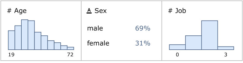
Visualization of data statistics. Displayed are two numerical features as histograms and the distribution percentages for a categorical feature.
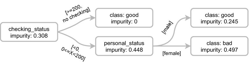
Visualization of a global surrogate. Displayed is a decision tree with five nodes to approximate an arbitrary black-box model. Each node contains either the feature used for this data split or in case of a leave node the majority class. Edges contain the conditions used for splitting the data.
For this study 36 participants with diverse backgrounds were recruited. Participants were acquired via a snowball sampling method, beginning with colleagues involved in data science, fellow researchers, contacts from research projects and company contacts. A total of of the participants assigned themselves the role data scientist, domain expert, and AutoML researcher. However, many participants also stated that a clear assignment to just one of these roles is difficult. A total of 44% of the participants worked in academia with 56% working in industry. The participants’ backgrounds can be further broken down into different professions: academia (25%), information technologies (22%), healthcare (17%), manufacturing (14%), robotics (8%), finance (8%), automotive (3%), and business administration (3%). In addition, participants were asked to rate their prior knowledge in ML and AutoML on a scale from 1 (very little) to 5 (very much). On average participants have an ML expertise of with several participants having no expertise with ML at all. Similarly, results for AutoML expertise () were also quite diverse with many participants having never heard of AutoML before. More information is available in Table 4 in the Appendix. In general, the group of participants was quite diverse with some participants having no prior experience using ML or AutoML and other participants being involved in either ML or AutoML or even both for many years.
Prior to the study, participants were informed about the nature of the study and its procedure. For the study itself, participants were invited to a roughly 20 minutes long online interview with one of the authors. First, demographics of the participants were collected. Next, as we did not expect all participants to have prior experience with AutoML, we provided a baseline AutoML interface based on screenshots of a commercial AutoML system excluding easily identifiable features like the company’s logo or name. The screenshots were presented and explained by one of the authors and covered the complete AutoML process from data import, manually selecting relevant features and the target feature, starting the optimization process, waiting for it to finish, and finally inspecting basic performance metrics of the created model. We also provided an introduction to AutoML from an end-user perspective while presenting the various screenshots. The goal was to familiarise participants with the high-level design goals of AutoML and to generate a general understanding of how AutoML can aid them in their work. The session was concluded by the actual card-sorting task using a collaborative website for brainstorming with sticky notes.
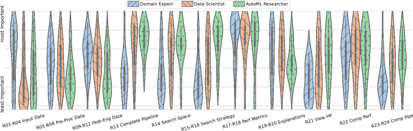
Results of the card sorting task. Fully described in the text and in Table 5.
Although participants were given the opportunity to add their own cards, only seven decided to use this option. Therefore, we first discuss the results of the pre-defined cards before considering the additional cards in more detail. Figure 2 provides the ranking of the importance of the predefined cards grouped by domain experts, AutoML researchers and data scientists. As expected, nearly all participants rank information about the final performance of a model, in textual (R17) or visual form (R18), as by far the most important information. Providing explanations for a model’s behaviour in form of local (R19) or global surrogates (R20), including the option to compare these values between different models (R22), is the second most important kind of information. Some information, like the ability to view the complete ML pipeline (R13) or compare different pipelines (R23), are more important to data scientists and AutoML researchers than domain experts. For the majority of cards, no clear preferences were found regarding the importance of the information we presented.
The seven additional cards cover three different topics. Five participants stated that they would like to modify candidates in-place to assess the impact of hyperparameters and different pipeline structures on the performance. Participant P5 expressed their desire to compare the created model with an analytical model, given that such a model already exists. P10 wanted to compare data produced by the different stages in an ML pipeline to validate that relevant information is still preserved.
3.3. Accommodating a Heterogeneous Target Audience
According to its self-proclamation, AutoML targets domain experts and data scientists (Zöller and Huber, 2021). A third (unintentional) user group is AutoML researchers and developers who spend considerable time studying various AutoML systems. Figure 2 shows that a clear distinction between the informational needs of domain experts, AutoML researchers and data scientists is not possible for most information. Even though slight differences between the three user groups are visible, those differences are often negligible or overlap significantly. Table 1 assigns the potential information to the user groups, given that significant differences in the importance exist. Only for eight cards, a significant difference () can be observed: Information about input data (R02 and R03) is more relevant for domain experts. Data scientists stated they would always perform an exploratory data analysis before building models with AutoML. Therefore, they do not require this information in an AutoML visualization. Furthermore, domain experts are significantly less interested in understanding and comparing pipeline structures (R13 and R23) and checking hyperparameters (R21) in comparison to the other two user groups. They primarily stated that knowing which algorithms are used in a pipeline would not be helpful as the background knowledge to interpret this information is missing. Finally, AutoML researchers were significantly more interested in a search space overview (R14) and search strategy visualizations (R15 and R16). For the remaining cards, the informational need does not correlate with one of the three roles but highly depends on the knowledge background of the person. Similar results were also observed in other studies (Drozdal et al., 2020; Crisan and Fiore-Gartland, 2021; Wang et al., 2021a).
| Information | DE | DS | AR | ||||
|---|---|---|---|---|---|---|---|
| DS | AR | DE | AR | DE | DS | ||
| R02 | View the meanings of columns in the raw input data | + | + | - | - | ||
| R03 | View statistics of raw input data | + | - | ||||
| R13 | View the complete processing pipeline | - | - | + | + | ||
| R14 | Know what the search space looks like | - | + | ||||
| R15 | Know how pipelines are chosen | - | - | + | + | ||
| R16 | Know how hyperparameters are chosen | - | - | + | + | ||
| R21 | View hyperparameters of model | - | + | ||||
| R23 | Compare differences between pipelines | - | - | + | + | ||
Current AutoML visual analytics tools always distinguish between either a domain expert, with no expertise in ML or programming, and a data scientist, who is only interested in technical model details but not the underlying domain (Cashman et al., 2019; Santos et al., 2019; Gil et al., 2019; Heyen et al., 2020; Gleicher et al., 2020; Wang et al., 2019a; Weidele et al., 2020; Park et al., 2021; Ono et al., 2021). We argue that the user basis is more diverse, with many shades between the classic domain expert and data scientist. Consequently, the visual analytics tool should not force users into either of the roles; rather, it should enable them to fully use their potential: A domain expert with no ML skills but knowledge in data visualization should be able to build their desired visualizations instead of being limited to the visual interface optimized for users with no technical experience. Instead of this one dimensional distinction of user groups, we propose to introduce three orthogonal knowledge dimensions related to the usage of AutoML: (1) Domain expertise for validating the predictions of a model, (2) MLexpertise for model improvement and behaviour validation, and (3) AutoMLexpertise for optimization refinement and debugging. As users can be proficient in multiple knowledge dimensions, eight different user groups can be deduced. It is important to note that all dimensions are continuous and no clear distinction between the eight user groups exists. Instead of creating dedicated visualizations for eight fluent, not clearly separable user groups, a visual analytics tool for AutoML should provide, to varying extents, useful information for all knowledge dimensions and users should be able to select relevant information.
For the context of this work, 53% of all participants have domain expertise, 75% ML expertise, and 28% AutoML expertise with 45% having only one proficiency and 55% having at least two proficiencies. For the remainder of this article we will refer to all participants being proficient in domain expertise as domain experts, independent of their other knowledge dimensions. The same holds true for data scientists and AutoML researchers.
3.4. Blending with the Data Science Workflow
To ease the use of the visual analytics tool, XAutoML should blend with the typical data science workflow. Wang et al. (2019b) proposed the data science workflow shown in Figure 3. This workflow contains three stages: preparation, modeling, and deployment, which can be further divided into 10 steps from data acquisition to runtime monitoring and model improvement. The execution of the steps data cleaning to model validation is usually an open-ended, exploratory and iterative process (Batch and Elmqvist, 2018; Cashman et al., 2019; Muller et al., 2019) which uses ad-hoc visual analytics extensively (Wang et al., 2019b). These visualizations enable practitioners to gain insights into their data and models quickly. In recent years, Jupyter has become the de-facto standard environment for such interactive visualization tasks (Rule et al., 2018; Drozdal et al., 2020).
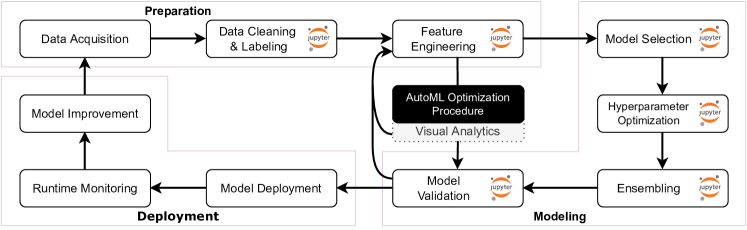
The usual data science workflow including a potential place for AutoML and the visual analytics. The ten different steps in the data science workflow are displace as circle and AutoML provides a shortcut between the steps feature engineering and model validation allowing users to skip three steps in the modeling phase. The visual analytics is intended as a direct extension to AutoML. In addition to the original data science workflow an additional branching from the visual analytics and model validation to feature engineering is added to indicate that modeling is an iterative procedure.
Jupyter Notebook (Kluyver et al., 2016) and its successor, JupyterLab (Project Jupyter, 2018), are web-based programming environments that support interactive data science and scientific computing. JupyterLab is built around the idea of computational notebooks, which combine code, execution results, and descriptive texts into a single file (Rule et al., 2018).
AutoML systems aim to (partially) automate the steps from feature engineering up to ensembling in the data science workflow. If AutoML would be more commonly used, it is reasonable to assume that it would be mainly used in the context of Jupyter as all surrounding steps in the workflow are also mostly executed in it. Instead of providing the visual analytics as a stand-alone external tool, it should be integrated with Jupyter to provide a cohesive environment for users (Crisan and Fiore-Gartland, 2021). This integration has an additional advantage: Data analytics range from simple statistical analysis to advanced ML techniques. It is virtually impossible for any single visual analytics tool to cover the complete range of possible analytics. Instead of pursuing this unreachable goal, we argue to provide easy options for experienced users to extend the visual analytics with their own ad-hoc visualizations in Jupyter. To encourage such behaviour, the tool should be designed as a data pipe in the data science workflow. In contrast to a data sink that only consumes data, namely the results of an AutoML optimization, a data pipe is able to emit new data the user can continue working with. Therefore, options for exporting (intermediate) datasets and ML artifacts should be implemented. Consequently, XAutoML could blend seamlessly with the data science workflow, as displayed in Figure 3.
Although Jupyter is a mighty tool for data scientists, programming skills are required to create notebooks, which makes it to a certain degree unsuitable for users with no programming skills. Following Grappiolo et al. (2019), we argue that Jupyter can become a useful tool for these users if additional visualization features are incorporated into notebooks that enable them to use Jupyter. Fortunately, JupyterLab provides a powerful extension application programming interface (API) that allows the inclusion of interactive JavaScript applications directly into notebooks. These extensions provide the opportunity to eliminate the prerequisite of programming skills, making Jupyter a usable environment for all types of users.
3.5. Visualization Needs and Design Goals
Based on the results from the initial requirements analysis and the literature review, we formulate three visualization needs, denoted as N1 to N3, that XAutoML aims to support. In addition, four non-functional design goals, denoted as G1 to G4, are listed.
N1. Effective and Efficient Validation of ML Models
The ability to understand and validate a model produced by AutoML is crucial for the prevalence of AutoML. If users decide not to use it due to missing trust in the results (Wang et al., 2019b), AutoML will fail to become relevant. Therefore, the primary goal of XAutoML is to provide necessary information to quickly assess the validity of single models and support users in selecting a model from the multitude of produced ones.
N2. Understanding and Diagnosing of AutoML Methods
AutoML methods are currently often designed as black-box optimizations. To provide a better understanding and interpretation of the complex and diverse optimization strategies in AutoML, we aim to provide an effective and intuitive visualization of (1) what the complete search space looks like, (2) how pipeline structures are synthesized, and (3) how hyperparameters are optimized. This visualization shall provide a rough understanding of the underlying search algorithm, without requiring extensive knowledge of AutoML.
N3. Search Space Refinements
As shown in Section 3.4, AutoML is usually used in an iterative workflow. Between two consecutive runs of AutoML, users have the option to adapt the underlying search space that is provided as a preset before performing the optimization. To effectively choose a refined search space, users should have information about which regions of the search space perform well and which regions can be pruned.
G1. Align with the Target Audience of AutoML
AutoML is aimed to assist domain experts and data scientists. Therefore, the visual analytics should also target these two groups. In addition, AutoML researchers should be able to extract useful information from the visual analytics.
G2. Blend with the Usual Data Science Workflow
We expect visual analytics to be constantly involved in the workflow of using AutoML. Therefore, it is crucial that the visual analytics blend seamlessly with the usual data science workflow. On one hand, this implies that output generated by an AutoML system has to be transferred easily to the visual analytics tool or that perhaps the visual analytics tool can be used to start an AutoML optimization. On the other hand, this implies that it has to be possible to transfer ML models back from the visual analytics tool to the usual data science environment, namely Jupyter.
G3. Always Provide more Detailed Information
The informational need of users is diverse. Following the idea of Five Whys (Serrat, 2017), XAutoML should provide information in a hierarchical fashion to prevent overloading users with unnecessary and undesired information. At the highest level, only very basic information should be available and users should have the option to dig deeper into certain analytics aspects to get more information. Ultimately, the visual analytics tool can not provide all the information required by a proficient user. Therefore, we aim to add options to break-out of XAutoML. This extends G2 by not only exporting selected models but also exporting artifacts related to models, e.g., intermediate datasets or sub-pipelines, for further manual inspection in Jupyter.
G4. Be Open to the AutoML World
The AutoML landscape is still rapidly developing and constantly shifting. To stay relevant, the visual analytics tool should not be coupled to a specific AutoML implementation. This implies that XAutoML should only depend on generic information provided by AutoML systems. Therefore, the common basis for the visual analytics and AutoML implementations should be scikit-learn (Pedregosa et al., 2011), NumPy (Van Der Walt et al., 2011) and pandas (McKinney, 2010), three commonly used libraries for ML in Python. Consequently, the visual analytics tool will be limited to scikit-learn pipelines for supervised classification on tabular data for now.
4. XAutoML: Exploring AutoML Optimizations
To fulfill the requirements, visual needs, and design goals identified in the previous section, we developed XAutoML. The interface of XAutoML is embedded in Jupyter and consists of an optimization overview, a candidate inspection to explore individual pipeline candidates, a search space inspection to gain insights about the optimization process and search space, and finally, an ensemble inspection view. The individual views are described in more detail in the following sections. Figure 4 provides an overview of XAutoML.
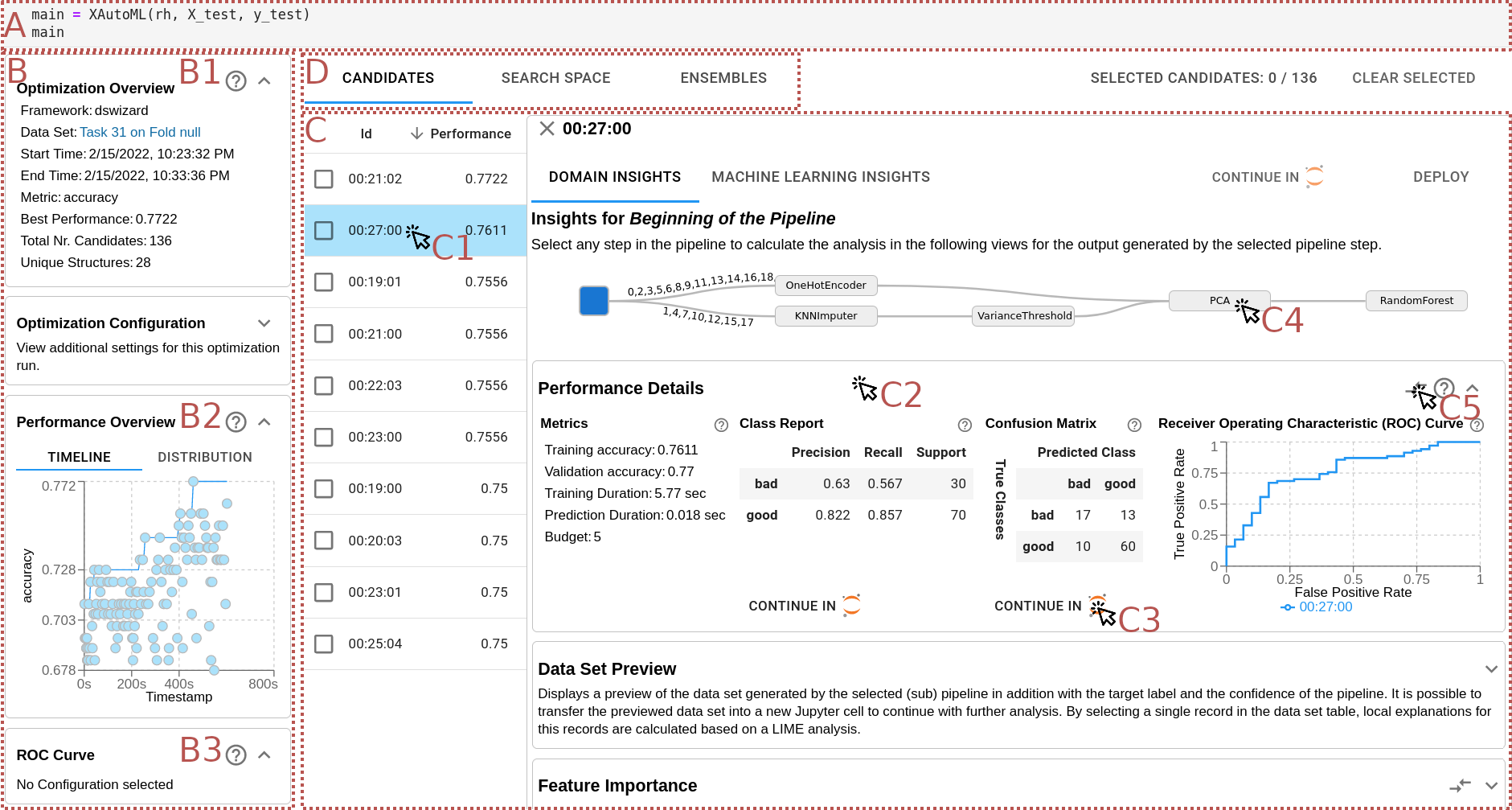
Screenshot of optimization overview and candidate inspection rendered in Jupyter. Fully described in the figure caption and in the text.
4.1. Optimization Overview
The optimization overview (Figure 4, B) provides an overview of the results of an AutoML optimization at a high level, including the total optimization duration, the number of evaluated candidates, and the performance of the best candidate. In addition, basic performance visualizations, namely the performance of all candidates over time and the number of candidates grouped by performance, are available. Users can select multiple candidates in the overview to compare their ROC curves. With these views, users can quickly identify interesting models for a detailed inspection. The candidate inspection view of interesting models can be opened directly from the overview.
4.2. Validating Machine Learning Models
The leaderboard (Figure 4, C) provides a tabular overview of all evaluated candidates. Each row displays the candidate id, performance (R17), average prediction time (currently not visible), and the used classifier (currently not visible) of a single candidate. Via the Continue in Jupyter button (currently not visible), the corresponding candidate can be exported to Jupyter. The leaderboard is intended to provide a rough first impression of the optimization with the option to select single candidates for further inspection.
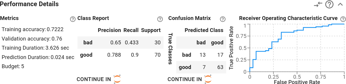
Screenshot of performance details view. Fully described in the text.
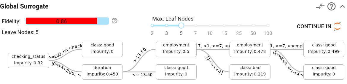
Screenshot of global surrogate view. Fully described in the text.
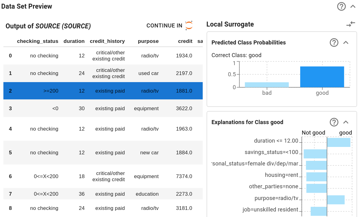
Screenshot of dataset preview view. On the left-hand side an extraction of the intermediate dataset is rendered as a table. On the right-hand side an optional assignment probability of the selected record to each potential class is displayed at the top. Down below the standard LIME visualization displaying the contribution of the various features to the predicted class is displayed.
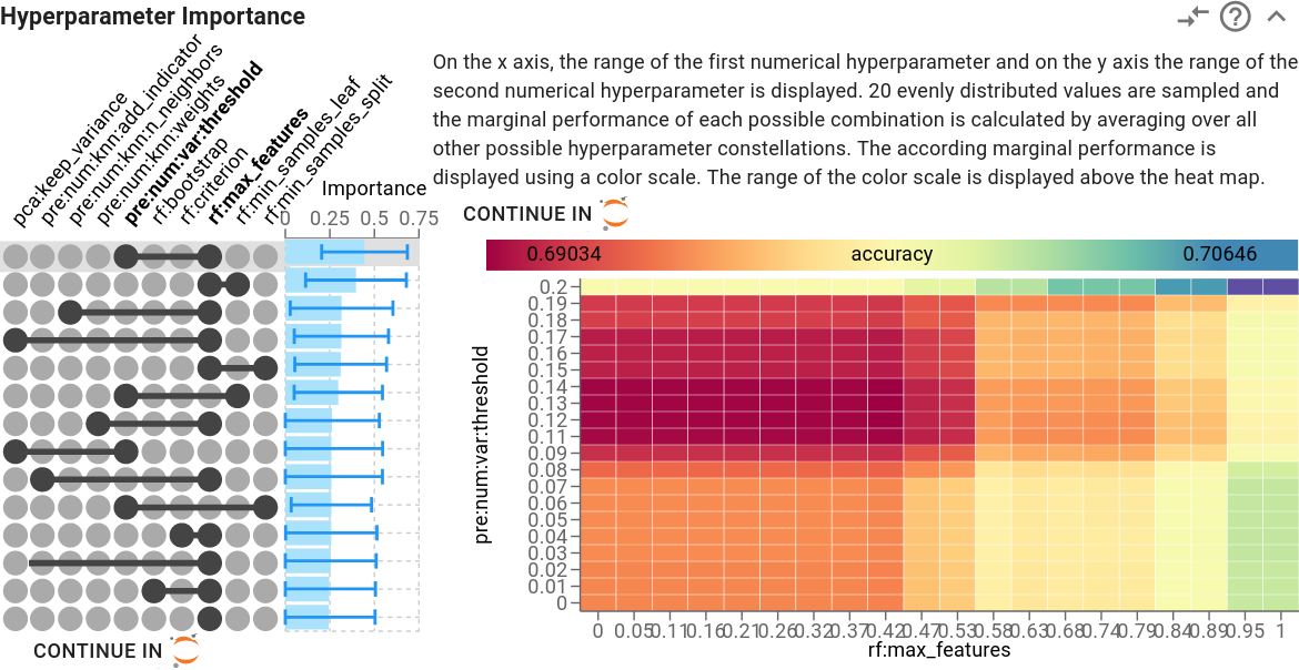
Screenshot of the hyperparameter importance view. On the left-hand side all hyperparameter (pairs) are listed sorted by their computed performance. The most important entry, the combination of two numerical hyperparameters, is selected. On the right-hand side, a heat map with the interactions of both selected hyperparameters is displayed. In addition, a description on how the read the heat map is given.
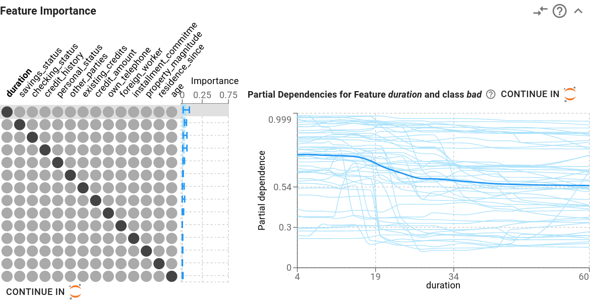
Screenshot of the feature importance view. On the left-hand side the same visualization as for the hyperparameter importance is used to list all features sorted by the importance. The most important feature is currently selected and the corresponding ICE and PDP plots on the right-hand side are given.
Users can reveal more details about candidates by selecting the corresponding entries in the leaderboard (Figure 4, C1). The candidate inspection view provides data and model transparency for a single ML pipeline. Users can find all required information to decide if the corresponding model is a “good” model worth selecting (N1). Therefore, existing XAI techniques are incorporated to provide a holistic visual user interface. Users can interactively control the level of detail they are interested in. The requirements analysis revealed no clear preferences regarding the presented information. Therefore, we decided to implement most of the model and data inspections and provide measures for users to visualize or extract the missing information on their own. Related information is aggregated in a card with a short description (Figure 4, C2) that can be revealed by selecting it. Figure 5 provides an overview of all implemented cards which are described in more detail later in this section. Inspections in each card are always computed based on the output of a single step in the pipeline. The complete pipeline structure is visible in a pipeline visualization view (Figure 4, C4). It renders all pipeline steps as a DAG that enables users to identify differences between the various candidates quickly (R13, R23). Even though the space for the pipeline visualization is quite limited, it is still sufficient to display typical pipelines constructed by modern AutoML systems containing at most 10 nodes and only a few parallel paths, e.g., (Feurer et al., 2015).
In Figure 4, a virtual data source node is currently selected and all inspections are calculated on the input data. Users can observe how the different steps in a pipeline affect the data by selecting the corresponding nodes in the pipeline visualization (Figure 4, C4) and inspecting the updated content of the different cards. The intention is to allow users to understand how each step in a pipeline modifies the input data. Each card provides at least one option to export the visualized data to Jupyter. Finally, users can also compare the information presented in a single card for various models (Figure 4, C5, R22, R23, R24).
The performance details view (Figure 5(a)) provides basic performance metrics (R17) and visualizations (R18). Displayed are training and test performance, duration of the training, duration of predicting new samples, and an optional multi-fidelity budget (Li et al., 2017) used for this model. The class report provides the precision and recall for each individual target class. In addition, a standard confusion matrix and ROC curve are displayed. This view shall enable users to assess the performance of an ML model in several dimensions. AutoML optimizes models against a single performance metric which may often be not enough to truly assess the predictive power and potential problems of a model. In addition, users can export the class report and confusion matrix to Jupyter for further analysis or visualization.
The global surrogate view (Figure 5(b)) fits a decision tree to the predictions of the selected candidate (R19). Users can interactively control the size of the decision tree by specifying the maximum number of leaf nodes, effectively weighting the explainability of the surrogate versus the fidelity to the black-box model. The fidelity bar provides an estimate of how good the decision tree resembles the actual model. The idea is to provide an easy option to generate an interpretable surrogate model with adaptable complexity. This may be used to validate and explain the behaviour of an ML model or even for legal auditions of it (Mohseni et al., 2021). Users can export the fitted decision tree to Jupyter for further analysis.
In the data set preview (Figure 5(c)), users can inspect the output dataset of the currently selected pipeline step (R1, R5, R9). This allows users to observe how each step in the pipeline modifies the input data and provides data transparency. Even without detailed understanding of each pipeline step, users may be able to deduce the rough impact of a step on the data. We deliberately decided not to support data visualizations. Study participants stated highly varying goals and desires for visualizations, covering gaining data insights, viewing statistical distributions, and generating cohorts for the analysis of FATE, just to name a few. Instead of providing only a limited data visualization—that would often be too restricted for users—, we rely on users to generate their own data visualizations in Jupyter and only provide tabular representations of the data. While this prevents users without knowledge in data visualization from visualizing the data, experienced users are not artificially limited by the visual analytics tool. Besides inspecting the tabular data, users can generate local surrogates (R20), computed via LIME (Ribeiro et al., 2016), for arbitrary records in the dataset. This provides a simple to understand attribution of feature values to the final prediction allowing users to gain insights into the model behaviour for single data instances to understand potential misclassifications.
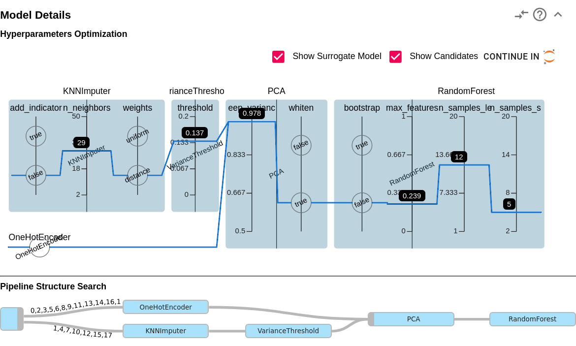
The selected hyperparameters of each step in the pipeline are listed in the model details view (Figure 5(d)). The hyperparameters are displayed in a CPC plot to visualize the respective search space (R14) and selected value for each hyperparameter (R21). In addition, the structure search graph at the time of sampling this pipeline structure is also displayed. More details regarding the CPC and structure search graph are available in Section 4.3.
Hyperparameters can have a significant impact on the performance of an ML model. In reality, only a few hyperparameters actually impact the performance significantly (Hutter et al., 2014) making it important to identify these. The hyperparameter importance view (Figure 5(e)) visualizes the importance of single hyperparameters and interactions between pairs of them (N3). The hyperparameter importance is calculated using fANOVA (Hutter et al., 2014). By selecting a hyperparameter, users get a detailed overview of well- and bad-performing regions in the search space. Using these visualizations, experienced users can extract valuable insights on how to modify the search space for the next optimization round by removing hyperparameters or adapting the search space limits.
Finally, the feature importance view (Figure 5(f)) reveals information about relevant features. Using a permutation feature importance (Breiman, 2001), the impact of each feature on the predictive power of the ML model is measured. Besides a ranking of all features, users can also view PDP and ICE plots. In case of a multi-class classification task, users can select the target class in PDP and ICE via a drop-down menu. This view should provide insights which features are important for the prediction and how feature values correlate with the predicted class. Both types of information can be used to validate the model behaviour.
4.3. Inspecting the AutoML Optimization Procedure
Besides validating models produced by AutoML, gaining insights to the actual AutoML optimization procedure was ranked as a desired information during the requirements analysis. This process transparency can help users to understand what the search space looks like, how different pipelines are chosen, and which strategy is used to optimize hyperparameters (N2). Furthermore, users are given information helping them to decide if the search space was sufficiently explored and the optimization algorithm is converging to a local minimum.
Pipeline Structure Search
A multitude of different search strategies have been proposed to synthesize pipeline structures. In general, pipeline structure search approaches can be divided into three different groups: (1) The simplest approaches use a fixed pipeline structure that does not change during the optimization. Instead, only the hyperparameters of the individual pipeline steps are fine-tuned. This pipeline structure is usually hand-crafted based on best-practices. (2) Template-basedapproaches also utilise a best-practise pipeline, but single steps in the pipeline are restricted to a set of algorithms instead of a fixed algorithm. The optimizer is allowed to, for example, pick a classification algorithm on its own instead of only tuning an SVM. (3) Approaches in the third group are able to build pipelines with flexible shape. The pipeline shape can be adopted to the given problem instance freely based on some internal optimization strategy.
For a user without strong AutoML expertise, it is often not obvious what the pipeline structure search space actually looks like and how the AutoML system traverses the search space. Consequently, users cannot easily deduce which kind of ML pipelines they can expect to be constructed by an AutoML optimizer. XAutoML provides a novel, intuitive visualization that allows users to grasp the general idea of the search procedure (R15), independent of the actual AutoML system. Therefore, we iteratively merge all constructed pipelines into a single structure search graph. Using a time-lapse function, users can observe how this structure search graph is constructed iteratively and can deduce the approximate search strategy and the corresponding structure search space. Figures 7 and 7 provide example visualizations for the template-based and flexible-shaped search strategies.

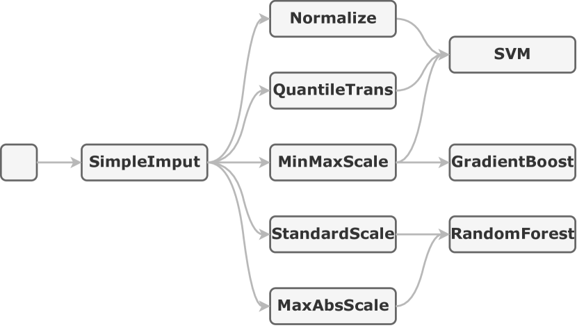
A template-based graph structure that becomes more complex with each iteration. In the first iteration, only a linear pipeline with three steps is displayed. After three iterations, the aggregated pipeline structure becomes more complex. The first pipeline step is still only a single algorithm, for the second step three alternatives can be selected, and for the last step two alternative are available. After the sixth iteration, the first step contains still only a single algorithm, but four and three different algorithms are available for the second and third step respectively.
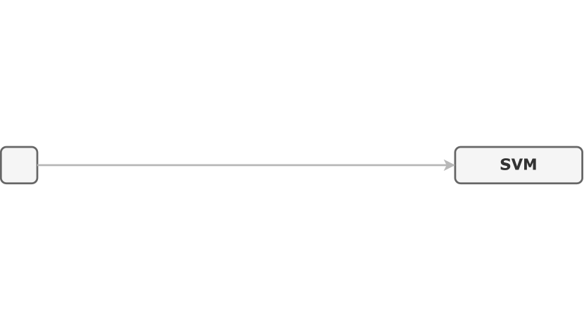
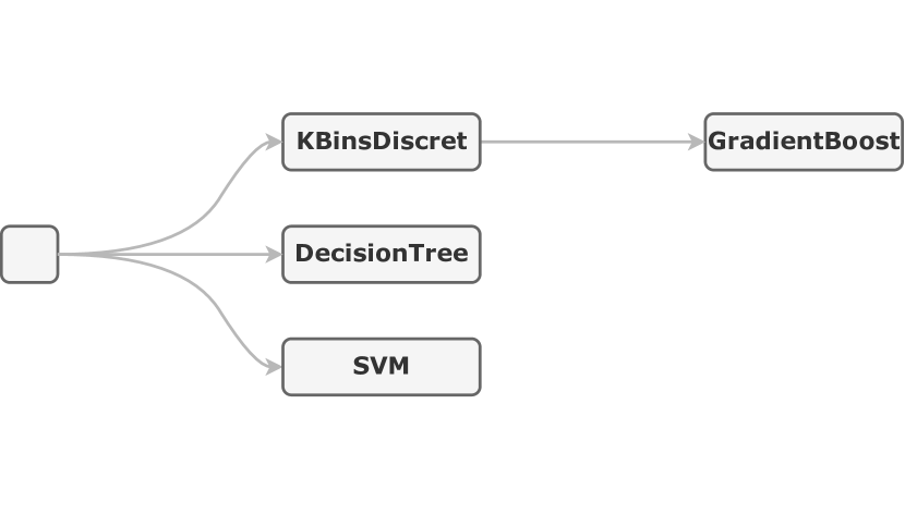
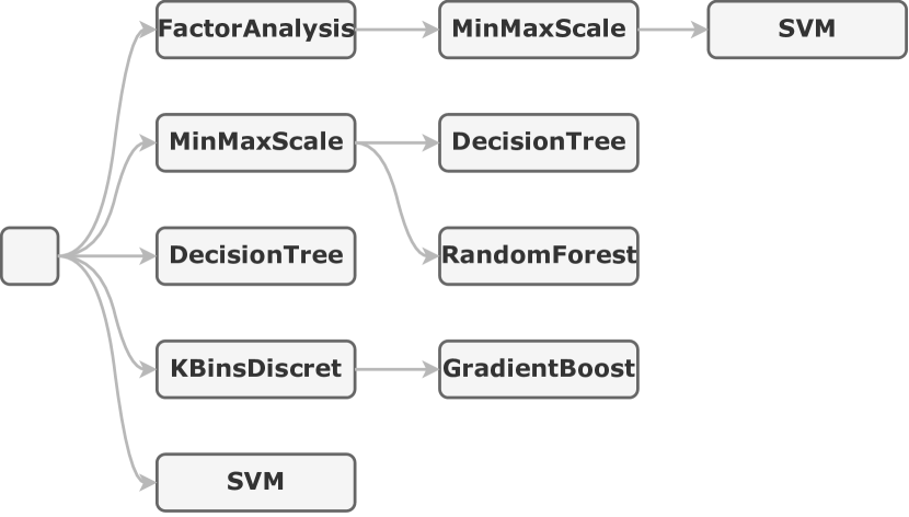
A flexible shaped graph structure that becomes more complex with each iteration. In the first iteration only a pipeline with a single step was produced. In the third iteration two pipelines with only a single step and one pipeline with two steps was produced. Finally, after six iterations, two pipelines with only one step, three pipelines with two steps, and a single pipeline with three steps were constructed.
Usually, a single ML pipeline is interpreted as a DAG in which each node is an ML primitive and edges indicate the flow of data between the primitives. ML pipelines often contain parallel paths, e.g., to use different pre-processing steps for numerical and categorical features. In the merged graph, it is not directly apparent if two child nodes of a node are actually part of the same pipeline using parallel paths or two different pipelines using identical steps at the beginning of the pipelines. A distinction between these two cases is important to correctly assess the pattern of constructed pipelines. In the case of parallel paths, we provide a visual guidance by adding the names of selected columns to out-going edges.
Merging two pipeline structures to a joint structure search graph can be interpreted as a bipartite graph matching problem. To merge two DAGs and , we use a simplified version of the graph matching algorithm proposed by Ono et al. (2021): Similar to computing the edit distance between two strings using dynamic programming, a cost matrix with all possible substitutions, additions, and deletions is constructed. Using the Hungarian algorithm (Kuhn, 1955), a mapping with minimal cost of rows to columns is computed. Two nodes are considered identical if they substitute each other, i.e., their substitution is selected in the cost matrix. and are merged by creating a compound node for identical nodes identified in the previous step and adding all remaining nodes from and to the new graph. Starting with the first two sampled pipeline structures, we repeat this procedure iteratively to merge the next pipeline structure into the joint structure search graph up to the currently selected timestamp in the time-lapse.
Conditional Parallel Coordinates for Non-Linear Pipelines
The conditional parallel coordinates (CPC) visualization proposed by Weidele et al. (2020) provides an intuitive way to inspect the hyperparameters of a complete ML pipeline. It is an extension of the original parallel coordinates visualization (Inselberg and Dimsdale, 1990) that allows users to interactively control the amount of information shown. Instead of showing all hyperparameters at once, CPC introduces different conditional layers of details. Users can drill down into particular steps of the ML pipeline (see Figure 8, A), revealing more details, namely all potential algorithms that can be used in this step, in form of a parallel coordinate plot (see Figure 8, B). Each algorithm can be expanded again to reveal its hyperparameters (see Figure 8, B1). For each hyperparameter a parallel coordinate axis is plotted containing the complete search space of it (see Figure 8, C). This hierarchical stacking of the axes fits naturally with AutoML search spaces. Search spaces are usually defined as tree structures due to conditional dependencies between hyperparameters (Hutter et al., 2009). To stick with the example in Figure 8, the pipeline highlighted in blue is configured to use a -Nearest Neighbors classifier. Consequently, the hyperparameters of a random forest classifier are inactive as they do not change the behaviour of the pipeline.
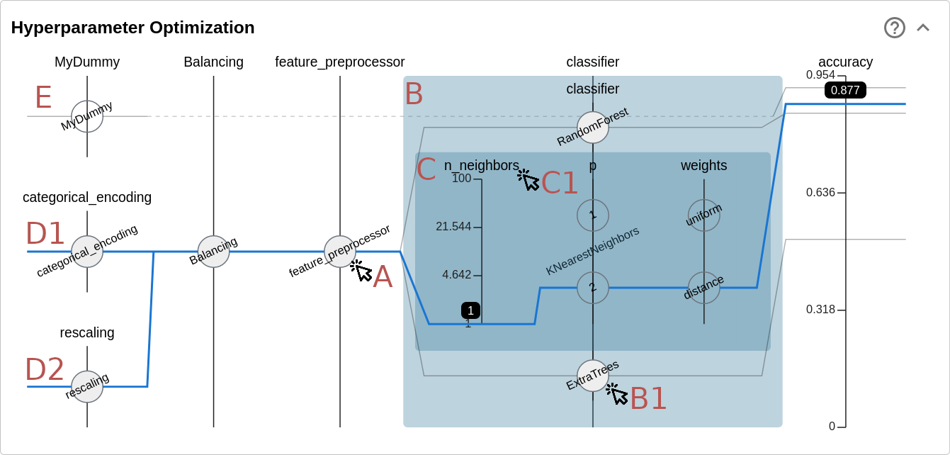
A conditional coordinate plot including all improvements proposed in the text. The CPC show a pipeline with a parallel path and in total eleven different steps. Two steps are expanded to reveal to available algorithms in these steps. In addition, the k-nearest neighbours classifier is expanded to reveal its three hyperparameters. The CPC plot contains multiple candidates and a single candidate, passing through all expanded axes is highlighted in blue.
The visualization proposed by Weidele et al. (2020) has two limitations, preventing the usage in combination with arbitrary AutoML systems. First, CPC requires a fixed number of coordinates present in all evaluated pipelines. This implies that all pipelines have to have the exact same number of steps. To resolve this limitation, we extend CPC by introducing the option to not provide values for selected coordinates. These missing values are indicated by a dashed line (see Figure 8, E). Second, CPC assumes a total order of pipeline steps. Yet, in reality, pipelines often contain parallel paths to use different pre-processing steps for categorical and numerical features. We extend CPC to support non-linear pipelines by splitting the vertical space into multiple simultaneous coordinates (see Figure 8, D1 and D2) for steps containing parallel paths. Consequently, the axes in CPC align with the actual pipeline shape again. This view should allow users to inspect the hyperparameter search space and sampled values of single hyperparameters for arbitrary complex pipeline structures.
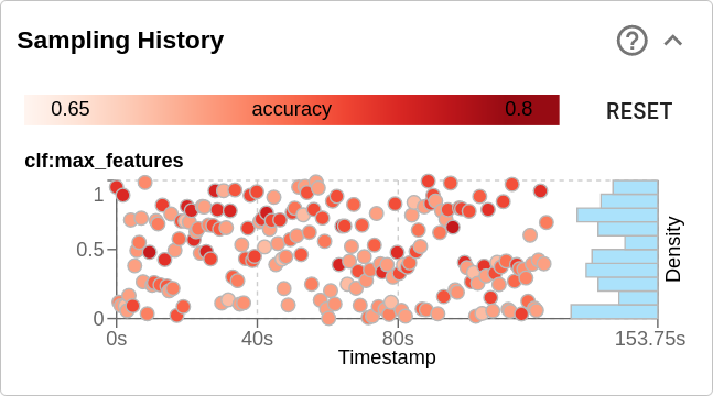
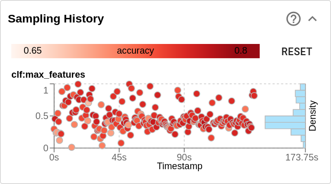
A visualization of sampled hyperparameter values over time using random search. The scatter dots are quite evenly distributed over the complete search space. The density histogram on the right-hand side of the scatter plots is roughly uniformly distributed.
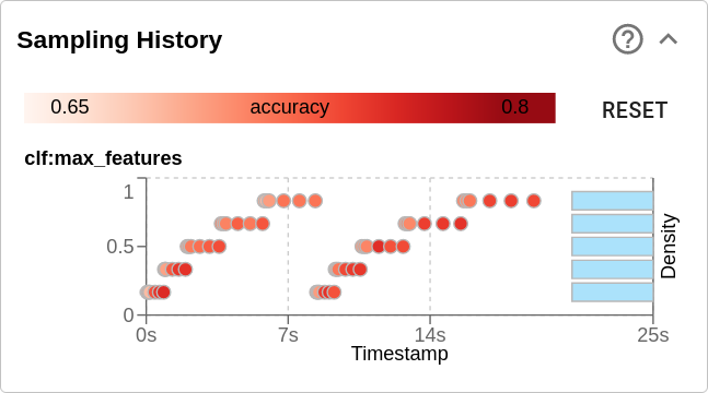
A visualization of sampled hyperparameter values over time using grid search. The scatter dots are perfectly evenly distributed over the complete search space. The density histogram on the right-hand side of the scatter plots shows a perfect uniform distribution of the sampled values.
A visualization of sampled hyperparameter values over time using Bayesian optimization. At the beginning of the optimization, the scatter dots are randomly distributed over the complete search space. After roughly 30 seconds of optimization, more values are around a specific value in the search space. In addition, some values are still sampled at random. The density histogram on the right-hand side of the scatter plots roughly resembles a uniform distribution. Only around the specific value, much more samples were generated.
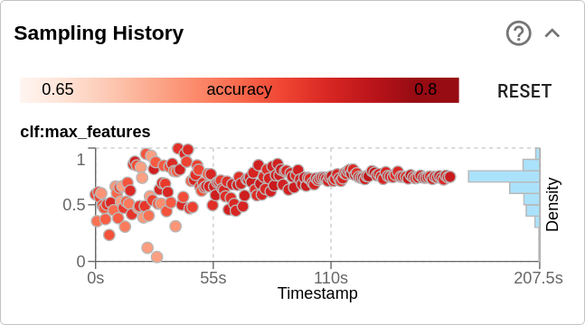
A visualization of sampled hyperparameter values over time using population-based optimization. At the beginning of the optimization, the scatter dots are randomly distributed over the complete search space. After roughly 50 seconds of optimization, the sampled values start to converge to a specific value in the search space. Over time, the variance in the sampled values becomes smaller and smaller. The density histogram on the right-hand side of the scatter plots roughly resembles a Gaussian distribution.
The CPC allows users to inspect single hyperparameters but the actual search strategy is not accessible as the sampling order of pipelines is not visible. To observe the sampling strategy of individual hyperparameters in a time-lapse (R16, N2), a sampling history view—inspired by the visualizations in HyperTendril (Park et al., 2021)—can be opened by selecting specific axes (see Figure 8, C1). The sampling history view, displayed in Figure 9, shows the sampled values of single hyperparameters over time. Each individual hyperparameter is visualized using a scatter plot: Each scatter point represents a single ML model, the -axis presents the timestamp at which the model was sampled, and the -axis represents the value of the selected hyperparameter. In addition, a color scale is used to encode the performance of each evaluated model such that users can confirm the optimization is converging to a local minimum. On the right-hand side, a histogram shows the distribution of sampled values over the possible search space. By selecting a scatter point, the details for the according model can be inspected. This view should allow users to deduce the rough hyperparameter search strategy. As an example, Figure 9 contains the visualization of four different search strategies that have very distinct sampling patterns. In addition, users can validate that indeed better models are found over time.
Finally, we integrate CPC with the remaining user interface. Users can highlight individual candidates for a more detailed inspection by brushing numerical axes or selecting a choice in categorical axes. Further details for interesting candidates identified in CPC can be accessed in the candidate inspection view by selecting the candidate.
Candidate Similarity and Search Space Coverage
Current AutoML systems do not provide measures for users to estimate the optimization progress. Users usually have to provide an optimization duration before starting the optimization but have no guidance on what duration is suited for their specific problem. An optimization duration is long enough if the search space was sufficiently explored and the optimizer converged to a local minimum. We propose a new procedure to visually inspect the coverage of an arbitrary AutoML search space, based on a non-linear metric in combination with multidimensional scaling (MDS) into two dimensions. A high-level overview of the procedure is given in Algorithm 1 and the final visualization in Figure 10.
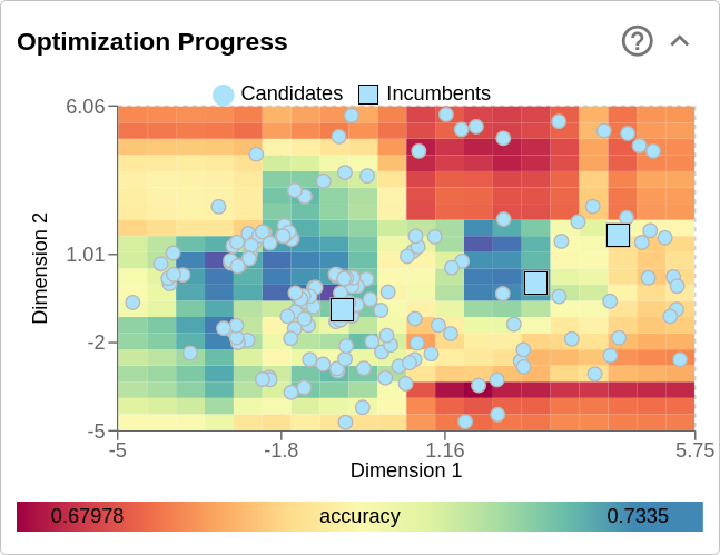
Visualization of the search progress using a scatter plot in combination with a heat map. The scatter dots are quite evenly distributed over the complete search space. At two points in the search space, clusters of scatter dots have formed. Those clusters are placed in regions which have a high accuracy according to the heat map indicating that the optimization has converged to a local minimum.
Given all previously evaluated candidates, their corresponding search space definitions, and their performances, we want to create a single plot that visualizes how well the search space was explored to provide guidance on a suitable optimization duration for users. As some AutoML systems use a progressive widening of the search space, e.g., (Zöller et al., 2021), a support of multiple search spaces is necessary. In the first step, we reuse the algorithm to merge different pipelines presented in the previous section to merge all hierarchical input search spaces into a single DAG . All existing candidates are padded with the default value of each newly introduced hyperparameter.
Next, boundary candidates are created with and being the lower and upper boundary of hyperparameter , respectively, and being the number of hyperparameters in . For high-dimensional search spaces this step is skipped due to the combinatorial explosion of possible candidates. Next, the pair-wise distances between all candidates are calculated respecting the tree-structured search space. Therefore, we assume that the importance of a hyperparameter is directly dependent on its depth in the hierarchical search space tree. The distance between two candidates is defined as a normalized heterogeneous euclidean distance weighted by as
| (1) |
For a numerical hyperparameter , is defined as
In case of being a categorical hyperparameter, is defined as
with being the indicator function.
Based on this distance matrix, all candidates are mapped into a 2d-space using an MDS. Furthermore, a regression model is fitted on the performance of the 2d candidates. This regression model is used to create a heat map showing the expected performance of the complete search space. In combination with an interactive time-lapse, users can check the sampled pipelines in the 2d representation over time. Virtually all modern AutoML optimizers combine an iterative exploration of the search space with an exploitation of knowledge about well-performing regions. If the optimization duration was too short, only exploration was performed. Consequently, the evaluated candidates would be scattered uniformly over the complete 2d representation. Once well performing regions have been identified, clusters of similar pipelines begin to form in the 2d representation. If these well-performing regions stop changing and only new points are added to the already existing clusters, without creating new clusters, increasing the optimization duration will probably not lead to significant performance improvements. Observing the sampled values in the time-lapse, users should be able to deduce a suitable cutoff duration for the optimization.
4.4. Ensemble Inspection
Many AutoML systems construct an ensemble of the best performing pipelines instead of yielding only the best candidate (Feurer et al., 2015; Olson and Moore, 2016; Zöller et al., 2021). Therefore, XAutoML provides an ensemble inspection view. This view contains the previously introduced candidate inspections for the complete ensemble. In addition, two visualizations are used to aid users in assessing the ensemble quality. We provide a tabular listing of all candidates in the ensemble with the according ensemble weighting. Users can open ensemble members in the candidate inspection view to get further details about the underlying ML model. In addition, users can compare the individual predictions of all ensemble members on any record in the input dataset. Finally, we provide a decision surface plot for all ensemble members and the complete ensemble. A decision surface is a hyper-plane separating data points in the input data space according to their predicted class label. By mapping these hyper-planes into a two-dimensional space via a principal component analysis (PCA) (Pearson, 1901) and using a color-coding for regions separated by decision surfaces, the decision making of a classifier can be visualized as a heat map. Even though these decision surface plots only provide a very rough impression of the actual decision making of the models, users can still get an impression of how the different ensemble members behave. The decision surface plots shall enable users to quickly identify interesting ensemble members that behave differently from the rest. Those models can then be inspected in more detail.
4.5. Dedicated Visualizations and Configuration
While the visualization shown in Figure 4 may provide a good opportunity for users to browse through all available information, it contains many superfluous information if a user is only interested in a specific subset of the available information. Therefore, XAutoML provides the option to render each of the visualizations presented in the previous sections in a dedicated Jupyter cell. Figure 11 shows an example of such a dedicated visualization.
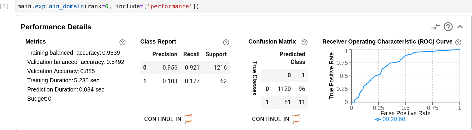
The performance details view described above is rendered in a dedicate Jupyter cell for the best performing pipeline candidate.
These dedicated visualizations are intended to allow experienced users of XAutoML to create visualization tailored to their very specific visualization needs. Splitting the visualization into smaller chunks may allow users to weave XAutoML into the computational narrative (Rule et al., 2018) of their notebook. As all visualizations are still part of XAutoML, users only interact with different views into the same underlying system exposing them to a consistent look and feel.
Similarly, specific information can also be excluded from XAutoML via simple configurations. For example, a domain expert can configure XAutoML to only display the optimization overview, leaderboard, performance details, dataset preview and global surrogates. Consequently, users without expertise in ML will not be exposed to technical ML details while still allowing them to explore the complete optimization.
4.6. Graphical Control Panel
Originally, XAutoML was intended to be only used by users with programming expertise within a Jupyter notebook. However, this would basically prevent users without programming skills from using XAutoML. Therefore, we also provide a simple control panel similar to Visus (Santos et al., 2019). This control panel allows users to upload a CSV file, select the target column from a tabular dataset preview and create an AutoML optimization procedure with according configurations through a graphical user interface. For now, only a limited set of AutoML frameworks with very basic configurations is supported. The optimization results are rendered in XAutoML, as described above, without the option to export insights as Python code to Jupyter.
4.7. Implementation Details
XAutoML is designed as a JupyterLab extension. The front-end is implemented in React (Meta Platforms Inc., 2013), Recharts (Recharts Group, 2015) and D3 (Bostock et al., 2011). The back-end, responsible for everything related to model evaluations, is implemented as a Python package using scikit-learn (Pedregosa et al., 2011), NumPy (Van Der Walt et al., 2011) and pandas (McKinney, 2010).
Execution results of AutoML systems—namely the fitted models, a description of the complete search space, and some minimal meta-information—can be imported into XAutoML via a small wrapper code. This code is responsible for translating the AutoML system specific formats to the one used by XAutoML. Developers of AutoML systems can provide adapters for their systems with roughly 100 lines of code. Supported AutoML systems are dswizard (Zöller et al., 2021), auto-sklearn (Feurer et al., 2015), grid and random search from scikit-learn (Pedregosa et al., 2011), FLAML (Wang et al., 2021c), and Optuna (Akiba et al., 2019). More AutoML systems may be added in future work.
To provide a seamless integration with Jupyter the imported execution results are rendered as a custom MIME type. The Jupyter extension connects this custom MIME type with the React application. In addition, the extension provides measures to export code snippets to new Jupyter cells which are used to extract artefacts from XAutoML and transfer them to Jupyter. Whenever the execution of Python code is necessary, e.g., for evaluating a single model, the extension provides a connection to the currently running user-kernel such that all code is executed in the same Python environment. The complete source code is publicly available on Github222 Available at https://github.com/Ennosigaeon/xautoml. and can also be installed easily via the Python package manager.
5. Evaluation
In this section, we demonstrate the usefulness and effectiveness of XAutoML in a user study. As discussed by Muller et al. (2019), many different roles are involved within data science projects. Similarly, AutoML also does not aim to support a single user group but tries to assist multiple roles. Accordingly, an evaluation of AutoML visualization methods should also be performed with multiple user groups. This user study was performed after the implementation of XAutoML was finished. We use the user study to answer the following three research questions:
- Q1:
-
Does XAutoML provide ML-related information understandable by a diverse user group?
- Q2:
-
Does XAutoML enable users with a diverse prior-knowledge of ML and the underlying domain to validate ML models?
- Q3:
-
Does XAutoML enable users with a diverse prior-knowledge of AutoML to understand AutoML optimizations?
5.1. Study Protocol and Participants
The user study was performed with the same 36 participants from the requirements analysis study in Section 3.2 in a semi-structured method after developing XAutoML. To answer the three research questions, we compared a set of items (displayed in Table 2) that participants were asked to answer for a baseline and for our proposed tool. These items aim to measure understanding of an AutoML optimization and trust in the constructed ML models. Identical input data was used to create the AutoML optimizations that are visualized in the baseline and our approach. All participants answered the items for both the baseline and our tool in a fixed order. In addition, for the proposed tool participants should solve a set of information retrieval tasks to control if participants were able to understand the provided visualizations. Participants were invited to a roughly 60 minutes long online interview with one of the authors. During the session, participants shared their computer screens and sessions were recorded. Participants were encouraged to speak freely in a think-aloud study, as it was done in other evaluations of visual analytics tools, e.g., (Wang et al., 2019a; Weidele et al., 2020; Ono et al., 2021; Park et al., 2021). We did not offer compensation for participating in the study. Each session consisted of four major phases:
-
(1)
First, we welcomed the study participants and introduced them to the background and goals of our study. In addition, this phase was used to gain a better understanding of the participants abilities. Participants were asked to introduce themselves and their daily work in regards to data analysis, ML and AutoML. Next, participants were asked to gauge their proficiency in the three aforementioned knowledge dimensions domain expertise, ML expertise and AutoML expertise. Therefore, participants were asked if they agree with the statement “I am a domain expert” on 4-point Likert scales with similar questions for ML and AutoML. Depending on their stated proficiency, participants were classified as either novices (strongly disagree and disagree) or experts (agree and strongly agree) in the respective area. In addition, participants without AutoML expertise were given a short, high-level introduction to AutoML from an end-user perspective to familiarise them with the goals and intended use cases of AutoML.
-
(2)
The second phase aimed at familiarizing the participants with the current state-of-the-art in AutoML. They were provided a filled Jupyter notebook containing a typical AutoML use-case333 Example notebooks are available with the source code. . First, basic information about the dataset was presented. The dataset was then used to train a classifier using auto-sklearn. Finally, the typical outputs produced by state-of-the-art AutoML systems, e.g., (Feurer et al., 2015; Olson and Moore, 2016; Wang et al., 2021c), namely a textual representation of the best pipeline, the test loss of the best pipeline, as well as a visualization of the training loss during the optimization were provided. Participants were guided through the notebook and given time to inspect the source code in detail if they wished to. Based on this information, participants were asked to provide a first evaluation of their understanding of AutoML to establish a baseline. Therefore, participants filled out a short questionnaire explained in more detail in Section 5.2 and displayed in Table 2.
-
(3)
Next, participants were asked to interact with XAutoML. To encourage the exploration of and to guide participants through the various aspects of XAutoML, participants were asked to solve small information retrieval tasks, which are described at the end of this section. A basic set of tasks covering all major parts of XAutoML should be solved by all participants. In addition, more tasks were added if users were experts in a specific area (see Phase 1). The tasks were designed to be solved by different visualizations and therefore guide the participants through all parts of XAutoML introduced in Section 4. The success or failure of solving each task was recorded by the interviewer. We reused the exact same input data from the second phase for all evaluations. After the participants had solved all assigned tasks, the understanding of AutoML methods was evaluated again using the exact same questionnaire as in Phase 2 with the goal to compare the answers before and after using XAutoML.
-
(4)
Afterwards, we wanted to test if the proposed option to create dedicated visualizations is useful for the participants. They were presented the options to configure XAutoML and render dedicated views. Using a 5-point Likert scale, participants were asked if this feature is helpful for them. Finally, the visual design and usability of XAutoML were recorded using the same 5-point Likert scale. In the end, participants were asked to reflect on any information that was missing in XAutoML. Therefore, participants were encouraged to examine the Jupyter notebook and XAutoML again. This opportunity was also used to let participants reflect on favored and unfavored elements of the proposed visual analytics tool. Finally, participants were given the chance to provide any remaining feedback freely.
Participants with domain expertise were provided with a dataset tailored to their professional background, instead of participants using their personal ones, to eliminate effects of different datasets. They were selected to be (1) a classification problem, (2) a relevant problem in the corresponding domain, (3) not trivially-solved by an ML algorithm, and (4) solvable by a domain expert. For example, participants with a healthcare background were asked to create an ML model predicting a high risk for a stroke based on 11 continuous and categorical features (Fedesoriano, 2021). Besides the raw data, participants were also provided with a description of all features and were allowed to familiarise themselves with the dataset. Participants without domain expertise were given one of the domain datasets at random.
The complete set of tasks participants solved in Phase 3 is listed in Table 6 in the Appendix. They can be split into four groups: (1) General Informationregarding the optimization, (2) Domain Expertisefor model validation and data insights, (3) MLExpertisefor model tuning, and (4) AutoMLExpertisefor optimization understanding. Each group contains tasks intended for all participants. In addition, a group may contain tasks requiring a profound prior knowledge in a knowledge dimension. Those tasks should only be solved by experts in the corresponding dimension.
5.2. Results and Participant Feedback
To answer our research questions, we analyze whether participants have a different understanding of the performed AutoML optimization and the generated ML models after using XAutoML in comparison to the baseline. We compared the answers to the questionnaire displayed in Table 2 that were given after using the baseline (Phase 2 of the study) with the answers after using the visual analytics tool (Phase 3 of the study). For each of the five questions in the questionnaire, the null hypothesis is “There is no difference in the answers after using the baseline and after using XAutoML” () for the current question under consideration. The alternative hypothesis is that the usage of XAutoML influenced the responses (). To compare the results, we performed two-sided -Tests (Student, 1908) with Holm-Bonferroni correction (Holm, 1979). We also provide effect sizes in terms of Cohen’s (Cohen, 1988).
| DE | DS | AR | All | ||
|---|---|---|---|---|---|
| Q11 | I understand how good the proposed model is. | ||||
| Q12 | I understand what the proposed model does. | ||||
| Q13 | I have enough information to decide if I want to use the model. | ||||
| Q14 | I have an idea what happened during the AutoML optimization. | ||||
| Q15 | I would trust a model constructed by AutoML. | ||||
Overall, XAutoML was able to increase the trust in AutoML systems significantly. On a scale from 1 (strongly disagree) to 5 (strongly agree), trust in ML models constructed by AutoML (Q15 in Table 2) increased from to , , 444 Given are mean standard deviation, the corrected -value, and the effect size in terms of Cohen’s (Cohen, 1988). after using XAutoML. Participants attributed the increased trust to a better understanding of the generated models and insights to the underlying optimization procedure. Accordingly, participants agreed to the statement that XAutoML is helpful for understanding and validating AutoML (). In the following, we take a closer look at how XAutoML improves process transparency and model validation. Furthermore, we discuss feedback provided by the participants. Details of all presented quantitative results are available in Tables 2 and 3.
Validating ML Models
Participants used XAutoML extensively to validate and compare ML models. Depending on their background in ML, different explanations were utilised. Unsurprisingly, users without knowledge in ML mainly focused on the performance metrics and global surrogates to gain insights into the behaviour of models. By inspecting multiple performance metrics on the train and test data in combination with the confusion matrix, users stated they received enough information to correctly assess the performance of a model (Q11, versus , , ). After picking a promising model, those users usually investigated the global surrogate to check if the model “does something sensible” (P23). Local surrogates and feature importance were consulted less often.
Experienced ML users did not focus on the global and local surrogates and feature importance. This can at least partially be attributed to the analysed dataset being selected at random. Consequently, those explanations had only minimal potential to provide new insights. Instead, participants focused more on gaining insights by inspecting the used algorithms in the different pipelines. ML practitioners liked the visualization of pipeline structures. The ability to observe changes in the data and the possibility to extract each intermediate dataset were considered very useful both for “visualizing the data” (P3) as well as “pipeline debugging” (P5). Some participants were able to detect ineffective or superfluous steps in the constructed pipelines using the intermediate datasets. Consequently, all participants were able to understand the behaviour of the constructed ML models significantly better using XAutoML (Q12, versus , , ) confirming research question Q2.
Understanding the AutoML Optimization Procedure
The second analytical need supported by XAutoML is aiding users in understanding the underlying AutoML search strategy and search space. Even though XAutoML was able to increase the understanding of the AutoML system (Q14, versus , , ), the results highly depend on the participant’s prior experience with ML. Users with little to no knowledge in ML had gained only minor insights into the AutoML procedures. They usually stated either missing knowledge in ML or math to understand the internals or were simply not interested in it.
In contrast, data scientists and AutoML researchers were able to gain insights into the AutoML optimization procedure. Even participants with no prior practical experience with AutoML were able to correctly identify and distinguish template-based, fixed, and flexible optimization strategies for pipeline structures. “The visualization is a good starting point to get into AutoML” (P32). Multiple users were surprised by the complexity of ML pipelines produced by some AutoML systems. “I thought AutoML is only good for hyperparameter optimization and pipeline construction is just a small extension” (P10).
Similarly, most users were able to correctly identify different hyperparameter search strategies like random search, grid search, or a model-based optimization. “Observing the search in a time-lapse is extremely helpful to understand the search algorithms” (P9). The combination of structure search graph and CPC enabled users to quickly identify the hyperparameters for each step in a potential ML pipeline. Nearly all users were able to formulate a rough concept of the underlying search space confirming research question Q3.
P12, an experienced AutoML user, highlighted the usefulness of the progress view for assessing the progress of the optimization run. “It is often quite hard to judge if the optimization has actually converged yet. The overview gives me this information at a glance” (P12). Yet, they also remarked that providing this information in real-time during the optimization procedure would be even more helpful. We discuss this issue of human guidance in Section 6.
AutoML in the Data Science Workflow
The integration with Jupyter and the option to export datasets and ML artifacts from XAutoML to Jupyter was received overwhelmingly positive. Only a single participant with programming skills said this integration is just a “nice gimmick” (P8) while all other participants highlighted the usefulness of this feature for their workflow. “Visualizations can only offer a subset of all potential analyses. Experts with domain knowledge are able to extract more information” (P2). Many participants confirmed our intended workflow presented in Section 3.4. They stated they could imagine using AutoML for creating an evaluation baseline in a new project they would aim to improve. Visual analytics are considered an integral part of AutoML. “Just because I was able to validate results in a single case, I will not trust AutoML in general” (P1). The current integration with Jupyter and the export of various artefacts from XAutoML does not force users to adapt their usual workflow. “There is simply no reason not to use the visualization” (P14). Unsurprisingly, the Jupyter integration was ignored by users without programming skills.
Grounding the Expectation in ML
An interesting effect we were able to observe is that participants’ proficiency in ML correlates negatively () with the understanding of what the proposed ML model does. Without providing additional explanations, participants with a low proficiency in ML reiterated the goal of the scenario when asked if they understood what the model does instead of questioning the actual behaviour of the ML model. Even when challenging this assumption, participants were still convinced that the provided ML model would solve their task. This is a good example of the risk of potentially “automating bad decisions” (Crisan and Fiore-Gartland, 2021) without noticing it by practitioners with minimal ML expertise. During the usage of XAutoML, most domain experts discarded the model initially suggested by the AutoML optimizer quickly using the global surrogate and performance metrics. Consequently, domain experts were able to identify invalid models, effectively preventing this pitfall.
Validating the Behaviour of the Search Algorithm
P11, an AutoML researcher, tested XAutoML with an AutoML system building increasingly more complex pipelines over time. The system uses an -greedy approach to explore new pipelines in the beginning of the optimization and picks from the already evaluated pipelines toward the optimization end. Using the time-lapse function of the structure search graph, P11 observed how during the first half of the optimization mostly new pipelines with increasing length are sampled, just as they expected. Yet, toward the end of the optimization, the search algorithm suddenly started favouring very short pipelines. Longer pipelines that were also previously evaluated are completely ignored. Confused by this observation, P11 checked the implementation of the search procedure after the user study and detected a bug enforcing the selection of the shortest possible pipeline in an exploitation step. Even though this information would have also been available by carefully studying the evaluated pipelines in the log file, XAutoML revealed this flaw in under two minutes.
Information Overload
In general, users were satisfied with the information presented in XAutoML as they had enough information to decide if they want to use a model constructed by AutoML (Q13, versus , , ). Even though not all information were relevant for all users, participants acknowledged the benefit of showing too much information instead of too little. “Users differ very much in their experience and knowledge. I like that people are able to pick the information they need” (P23). Furthermore, the information were presented in an understandable way as participants were able to solve of the given tasks with no big differences between tasks for all users () and expert-only tasks (). However, the current way of providing the information in XAutoML can still be improved. Multiple participants, with diverse proficiencies, remarked a visual information overload (Poursabzi-Sangdeh et al., 2021) during the first minutes of the user study. “There are too many features to grasp the complete program immediately” (P3). Yet, on average, participants agreed to the statements that the visual design is easy to learn () and understand (). From these apparently contradicting statements, we deduce that a better structuring of the presented information is necessary. Consequently, the research question Q1 is only partially fulfilled.
| DE | DS | AR | All | ||
|---|---|---|---|---|---|
| Q21 | The visual design is easy to learn. | ||||
| Q22 | The visual design is easy to understand. | ||||
| Q23 | XAutoML provides sufficient details for me. | ||||
| Q24 | XAutoML helps me to understand and validate AutoML. | ||||
| Q25 | XAutoML helps me with my computational narrative. | ||||
| Q26 | The configuration of XAutoML is helpful for me. |
Dedicated Views and Configuration
The option to render dedicated views of XAutoML received mixed ratings from the participants. Some data scientists highlighted the usefulness for presentations (P27, P30) or training (P31) while others ignored it. Most AutoML researchers and domain experts simply did not intend to use Jupyter for documentation or narrative purposes. Yet, as this feature is completely optional, on average, participants had a neutral feeling () about it. Similarly, participants had mixed feelings about the usefulness of configuring the displayed information in XAutoML (). While participants being proficient in only a single knowledge dimension acknowledged the benefits from hiding irrelevant information, other participants were indifferent to this option. In contrast, some participants even disliked it because they want to browse through all available information.
5.3. System Usability
The usability of XAutoML is evaluated using the system usability score (SUS) (Brooke, 1996). To compute the SUS, participants were asked to fill out the standard SUS survey at the end of the user study. The SUS contains 10 questions participants were asked grade on a scale of (strongly disagree) to (strongly agree) and ranks a system on a scale from 0 to 100. Our system reached points with detailed results being available in Table 7 in the Appendix. According to Bangor et al. (2008), this grades the usability of XAutoML in the middle region of Good making it acceptable. Domain experts ranked the system worse () than data scientists () or AutoML researchers (). The major criticism of participants was that they had problems imagining most people would learn to use the system quickly ( of possible points). We attribute this assessment to the information overload experienced by participants.
6. Discussion & Future Work
Study participants were interested in validating the behaviour of single ML models and/or understanding the internals of the AutoML optimization. This confirms our identified visualization needs N1 and N2. It is important to note that these two needs do not correlate with the traditional user groups of data scientists and domain experts but depend on a more diverse personal background knowledge of each participant.
Interestingly, most participants with ML expertise considered AutoML only as a baseline method for ML. Instead of using a proposed model directly, they wanted to build a custom model manually improving on the performance yielded by AutoML. A potential explanation could be that most study participants had no prior experience with AutoML and were therefore satisfied with AutoML building “good enough models” (P3) for a baseline. Finding the best possible ML model via AutoML was not a goal of the participants. Consequently, a search space refinement—and therefore identifying well-performing regions in the search space—for consecutive optimization runs was not interesting for the study participants. This contradicts our identified visualization need N3. Further research with users having a wider spectrum of prior knowledge in AutoML is necessary to validate our identified analytical needs.
Instead of designing XAutoML for a single user group, we decided to provide a lot of information and rely on users to pick the relevant and ignore the rest. The user study showed that participants from all three knowledge dimensions were able to extract relevant information from XAutoML supporting our design goal G1. Furthermore, study participants having programming skills highlighted the benefits of integrating XAutoML with Jupyter. Extracting data from the visual analytics for further manual analysis was considered an integral part for incorporating AutoML and the visual analytics into the usual workflow of the participants confirming design goals G2 and G3. Finally, AutoML systems can be integrated with XAutoML easily as only minimal information has to be provided by the AutoML system supporting our design goal G4. To prove this claim, XAutoML is currently able to visualize the results of five AutoML libraries.
As an alternative to using only a single visualization system, it would also have been possible to create multiple systems specialized for specific user groups, i.e., users with identical knowledge dimensions. We consider this approach suboptimal for several reasons: (1) A dedicated visualization for each knowledge dimension would expose users to up to three different systems. From a users perspective it is cumbersome to switch between different systems to collect information about basically one object of interest. (2) The requirements engineering revealed that even within only a single user group, e.g., pure domain experts, a clear preference which information should be available is not visible. This would expose users to undesired information even with multiple systems. (3) Some information can only be extracted when considering multiple knowledge dimensions at once, e.g., the impact of different preprocessing strategies on certain features related to FATE. This combination of insights would be hard to achieve with distinct systems. Even though one size fits all visualizations are extremely difficult to design in the context of AutoML, we still argue that a single system with the option to hide undesired information is the best compromise between overwhelming users with too many information and limiting users by not providing relevant information.
6.1. Current Limitations
Many participants stated that they were overwhelmed by the amount of different information presented in the visualization. This was the major criticism of XAutoML. We tried to prevent this visual information overload by designing XAutoML to provide information in different levels of details supporting our design goal G3. Yet, apparently, the current visual design fails at this task at least partially. This initial shock was usually overcome within roughly minutes of participants interacting with XAutoML. Further analysis on how to restructure the presented information and visualizations is necessary. During the study several participants suggested introducing additional layers to expose users to less information at once. Alternatively, it would be interesting to let users interact with pre-defined configurations of XAutoML tailored to their knowledge dimensions to show less information at once.
XAutoML is currently designed to create post-hoc explanations. Users can only analyse the results of an AutoML optimization run after it has finished. Based on the extracted insights, users can adapt the search space and dataset to guide the next optimization run into the right direction. From a user’s perspective, this workflow can be cumbersome as the lengthy completion of the AutoML optimization has to be awaited. In the spirit of human-guided ML, a tight coupling between AutoML system and visual analytics is highly desirable (Gil et al., 2019) to control the optimization procedure and modify the search space in-place during the optimization. Yet, this directly conflicts with the design goal to support many AutoML systems. In addition, it exposes users to internal information of the AutoML optimizer that could be hard to understand for end-users. On the other hand, multiple AutoML researchers requested exactly these internals for detailed system debugging. Further research is required to distill common user interactions with AutoML systems to a standardized framework coupling visual analytics and optimizer.
As a consequence of the post-hoc explanations and the abstraction of the underlying AutoML system, most visualizations are computed on the fly. These ad-hoc computations become quite time-consuming for large datasets, severely limiting the user experience. Even though all computed results are cached and the input data for costly operations is down-sampled, the initial computation of the requested data may still require too much time for an interactive system. Another drawback of being AutoML systems agnostic is the lack of information about the internal optimizer reasoning. XAutoML only provides visualizations based on the evaluated models over time. Given this information, users of XAutoML are able to make an educated guess about the internal reasoning of the AutoML optimizer. It would be better if AutoML systems provide more inherent information to explain their behaviour, but unfortunately, this is simply not the case with current state-of-the-art AutoML systems.
Multiple participants remarked that relevant information, they were looking for, was not easy to find due to a discrepancy in the used terminology. XAutoML uses established terms from ML, yet participants are often not familiar with ML and use other terms for the same concept, e.g., recall for binary classification and sensitivity. The effort to mentally map to known terms made usage of XAutoML unnecessary straining for some participants.
During the study, multiple study participants were interested in filtering the displayed ML candidates by various factors for further analysis. For example, participants wanted to use the importance of specific features for the analysis of FATE or the confidence of model predictions. Currently, it is not possible to filter candidates at all to ease the analysis.
In the user study, we compared XAutoML with a pure programmatic method of using AutoML in Jupyter. A comparison with an existing visual analytics tool as a baseline was not performed. Consequently, the observed improvements could potentially be attributed to the pure existence of (simple) visualizations and not the concrete design of XAutoML. Further insights, if similar improvements could be achieved with simpler approaches would be helpful to steer the future development of visual analytics tools for AutoML.
6.2. Future Work
During the user study, many users voiced their desire to create specific ML models based on the insights extracted from their detailed analysis of ML models, e.g., giving a higher importance to a specific feature. Gil et al. (2019) have analysed common requirements for human-guided ML. An option to incorporate human guidance into a running AutoML optimization, building single models specifically requested by the user, would be useful.
Currently, XAutoML provides the same visualizations for all ML pipelines. Yet, some XAI techniques are only applicable to specific ML models, e.g., attention mechanisms for neural networks. By considering the actual ML model of a pipeline, it would be possible to include additional model-specific visualizations.
XAutoML is currently limited to classification tasks on tabular data. An extension to further learning tasks and data types is desirable and was requested during the user study by multiple participants. Similarly, we plan the inclusion of further AutoML systems to increase the potential user basis of XAutoML.
Finally, we only considered the interaction of a single user with XAutoML. However, in practice data science tasks are often solved by cross-functional teams. It would be interesting to evaluate in further studies how XAutoML could be used to assist multiple users.
7. Conclusions
We presented XAutoML, an open-source visual analytics tool for understanding and validating AutoML procedures by making AutoML optimizations transparent and explaining ML models produced by AutoML. In a requirement analysis study, we have collected desired explanations and information from a diverse user basis containing 16 data scientists, 11 domain experts, and 9 AutoML researchers. The results indicate that designing visual analytics tools focused on a single user group is, in the context of AutoML, not helpful. A clear assignment of explanations to specific user groups is often not possible. XAutoML allows users to pick interesting information from a broad spectrum. In a user study, we were able to prove the effectiveness and usefulness of XAutoML. Our results showed that the usage of XAutoML significantly increased the understanding of AutoML systems and ML models produced by them leading to an increased trust of users in AutoML.
Acknowledgements.
The authors wish to thank the participants of the requirements analysis and the user study for their time and valuable input. This work was partially supported by the German Federal Ministry for Economic Affairs and Climate Action in the project FabOS (project no. 01MK20010N), by the German Federal Ministry of Education and Research in the project RESPOND (project no. 01—S8067A) and by the Baden-Wuerttemberg Ministry for Economic Affairs, Labour and Tourism in the project KI-Fortschrittszentrum “Lernende Systeme und Kognitive Robotik” (project no. 036-170017).References
- (1)
- Akiba et al. (2019) Takuya Akiba, Shotaro Sano, Toshihiko Yanase, Takeru Ohta, and Masanori Koyama. 2019. Optuna : A Next-generation Hyperparameter Optimization Framework. In International Conference on Knowledge Discovery and Data Mining. Association for Computing Machinery, 2623–2631.
- Alaa and Schaar (2018) Ahmed M. Alaa and Mihaela Van Der Schaar. 2018. AutoPrognosis: Automated Clinical Prognostic Modeling via Bayesian Optimization with Structured Kernel Learning. In International Conference on Machine Learning, J. Dy and A. Krause (Eds.). PMLR, 139–148.
- Bangor et al. (2008) Aaron Bangor, Philip T. Kortum, and James T. Miller. 2008. An Empirical Evaluation of the System Usability Scale. International Journal of Human-Computer Interaction 24, 6 (2008), 574–594.
- Batch and Elmqvist (2018) Andrea Batch and Niklas Elmqvist. 2018. The Interactive Visualization Gap in Initial Exploratory Data Analysis. IEEE Transactions on Visualization and Computer Graphics 24, 1 (2018), 278–287.
- Bergstra et al. (2011) James Bergstra, Rémi Bardenet, Yoshua Bengio, and Balázs Kégl. 2011. Algorithms for Hyper-Parameter Optimization. In Advances in Neural Information Processing Systems. Curran Associates, Inc., 2546–2554.
- Biedenkapp et al. (2018) André Biedenkapp, Joshua Marben, Marius Lindauer, and Frank Hutter. 2018. CAVE: configuration assessment, visualization and evaluation. In International Conference on Learning and Intelligent Optimization, R. Battiti, M. Brunato, I. Kotsireas, and P. M. Pardalos (Eds.). Springer International Publishing, 115–130.
- Bostock et al. (2011) Michael Bostock, Vadim Ogievetsky, and Jeffrey Heer. 2011. D3: Data-Driven Documents. IEEE Transactions on Visualization and Computer Graphics 17, 12 (2011), 2301–2309.
- Breiman (2001) Leo Breiman. 2001. Random Forests. Machine Learning 45, 1 (2001), 5–32.
- Brooke (1996) John Brooke. 1996. SUS: A ’Quick and Dirty’ Usability Scale. Usability Evaluation In Industry 189, 194 (1996), 4–7.
- Burkart and Huber (2021) Nadia Burkart and Marco F. Huber. 2021. A Survey on the Explainability of Supervised Machine Learning. Journal of Artificial Intelligence Research 70 (2021), 245–317.
- Cashman et al. (2019) Dylan Cashman, Shah Rukh Humayoun, Florian Heimerl, Kendall Park, Subhajit Das, John Thompson, Bahador Saket, Abigail Mosca, John Stasko, Alex Endert, Michael Gleicher, and Remco Chang. 2019. A User-based Visual Analytics Workflow for Exploratory Model Analysis. Computer Graphics Forum 38, 3 (2019), 185–199.
- Chen et al. (2018) Boyuan Chen, Harvey Wu, Warren Mo, Ishanu Chattopadhyay, and Hod Lipson. 2018. Autostacker: A Compositional Evolutionary Learning System. In Genetic and Evolutionary Computation Conference. Association for Computing Machinery, 402–409.
- Clouder (2018) Alibaba Clouder. 2018. Shortening Machine Learning Development Cycle with AutoML. Retrieved 01/03/2019 from https://www.alibabacloud.com/blog/shortening-machine-learning-development-cycle-with-automl_594232
- Cohen (1988) Jacob Cohen. 1988. Statistical Power Analysis for the Behavioral Sciences. Lawrence Earlbaum Associates. 20–26 pages.
- Crisan and Fiore-Gartland (2021) Anamaria Crisan and Brittany Fiore-Gartland. 2021. Fits and Starts: Enterprise Use of AutoML and the Role of Humans in the Loop. In Conference on Human Factors in Computing Systems. Association for Computing Machinery, 1–15.
- Das et al. (2020) Piali Das, Valerio Perrone, Nikita Ivkin, Tanya Bansal, Zohar Karnin, Huibin Shen, Iaroslav Shcherbatyi, Yotam Elor, Wilton Wu, Aida Zolic, Thibaut Lienart, Alex Tang, Amr Ahmed, Jean Baptiste Faddoul, Rodolphe Jenatton, Fela Winkelmolen, Philip Gautier, Leo Dirac, Andre Perunicic, Miroslav Miladinovic, Giovanni Zappella, Cedric Archambeau, Matthias Seeger, Bhaskar Dutt, and Laurence Rouesnel. 2020. Amazon SageMaker Autopilot: A White Box AutoML Solution at Scale. In Data Management for End-to-End Machine Learning. Association for Computing Machinery, 1–7.
- Dataiku (2021) Dataiku. 2021. Dataiku. Retrieved 16/10/2023 from https://www.dataiku.com
- DataRobot (2021) DataRobot. 2021. AI Cloud. Retrieved 30/12/2021 from https://www.datarobot.com/platform/
- Doran et al. (2017) Derek Doran, Sarah Schulz, and Tarek R. Besold. 2017. What Does Explainable AI Really Mean? A New Conceptualization of Perspectives. In Workshop on Comprehensibility and Explanation in AI and ML, T. R. Besold and O. Kutz (Eds.). CEUR-WS.org, 1–8.
- Drori et al. (2018) Iddo Drori, Yamuna Krishnamurthy, Remi Rampin, Raoni de Paula Lourenco, Jorge Piazentin Ono, Kyunghyun Cho, Claudio Silva, and Juliana Freire. 2018. AlphaD3M: Machine Learning Pipeline Synthesis. In International Conference on Machine Learning AutoML Workshop. 1–8.
- Drozdal et al. (2020) Jaimie Drozdal, Justin Weisz, Dakuo Wang, Gaurav Dass, Bingsheng Yao, Changruo Zhao, Michael Muller, Lin Ju, and Hui Su. 2020. Trust in AutoML: Exploring Information Needs for Establishing Trust in Automated Machine Learning Systems. In International Conference on Intelligent User Interfaces. Association for Computing Machinery, 297–307.
- Erickson et al. (2020) Nick Erickson, Jonas Mueller, Alexander Shirkov, Hang Zhang, Pedro Larroy, Mu Li, and Alexander Smola. 2020. AutoGluon-Tabular: Robust and Accurate AutoML for Structured Data. In International Conference on Machine Learning AutoML Workshop. 1–28.
- Falkner et al. (2018) Stefan Falkner, Aaron Klein, and Frank Hutter. 2018. BOHB: Robust and Efficient Hyperparameter Optimization at Scale. In International Conference on Machine Learning, J. Dy and A. Krause (Eds.). PMLR, 1437–1446.
- Fedesoriano (2021) Fedesoriano. 2021. Stroke Prediction Dataset. Retrieved 29/12/2021 from https://www.kaggle.com/fedesoriano/stroke-prediction-dataset
- Feurer et al. (2015) Matthias Feurer, Aaron Klein, Katharina Eggensperger, Jost Tobias Springenber, Manuel Blum, and Frank Hutter. 2015. Efficient and Robust Automated Machine Learning. In International Conference on Neural Information Processing Systems, C. Cortes, D. D. Lee, M. Sugiyama, and R. Garnett (Eds.). MIT Press, 2755–2763.
- Freitas (2019) Alex A. Freitas. 2019. Automated Machine Learning for Studying the Trade-Off Between Predictive Accuracy and Interpretability. In Machine Learning and Knowledge Extraction, A. Holzinger, P. Kieseberg, A M. Tjoa, and E. Weippl (Eds.). Springer International Publishing, 48–66.
- Friedman (2001) Jerome Friedman. 2001. Greedy Function Approximation : A Gradient Boosting Machine. The Annals of Statistics 29, 5 (2001), 1189–1232.
- Gil et al. (2019) Yolanda Gil, James Honaker, Vito D Orazio, Daniel Garijo, and Neda Jahanshad. 2019. Towards Human-Guided Machine Learning. In International Conference on Intelligent User Interfaces. Association for Computing Machinery, 614–624.
- Gleicher et al. (2020) Michael Gleicher, Aditya Barve, Xinyi Yu, and Florian Heimerl. 2020. Boxer: Interactive Comparison of Classifier Results. In Computer Graphics Forum, H. Hauser and P. Alliez (Eds.). Wiley, 181–193.
- Goldstein et al. (2015) Alex Goldstein, Adam Kapelner, Justin Bleich, and Emil Pitkin. 2015. Peeking Inside the Black Box: Visualizing Statistical Learning With Plots of Individual Conditional Expectation. Journal of Computational and Graphical Statistics 24, 1 (2015), 44–65.
- Golovin et al. (2017) Daniel Golovin, Benjamin Solnik, Subhodeep Moitra, Greg Kochanski, John Karro, and D. Sculley. 2017. Google Vizier: A Service for Black-Box Optimization. In International Conference on Knowledge Discovery and Data Mining. Association for Computing Machinery, 1487–1495.
- Google LLC (2022) Google LLC. 2022. Google Search Trends. Retrieved 16/10/2023 from https://trends.google.com/trends/explore?date=today5-y&q=automl,machinelearning
- Grappiolo et al. (2019) Corrado Grappiolo, Emile Van Gerwen, Jack Verhoosel, and Lou Somers. 2019. The Semantic Snake Charmer Search Engine: A Tool to Facilitate Data Science in High-tech Industry Domains. In Conference on Human Information Interaction and Retrieval. Association for Computing Machinery, 355–359.
- H2O.ai (2019) H2O.ai. 2019. H2O AutoML. Retrieved 08/11/2019 from http://docs.h2o.ai/h2o/latest-stable/h2o-docs/automl.html
- Heyen et al. (2020) Frank Heyen, Tanja Munz, Michael Neumann, Daniel Ortega, Ngoc Thang Vu, Daniel Weiskopf, and Michael Sedlmair. 2020. ClaVis: An Interactive Visual Comparison System for Classifiers. In Conference on Advanced Visual Interfaces. Association for Computing Machinery, 1–9.
- Holm (1979) Sture Holm. 1979. A Simple Sequentially Rejective Multiple Test Procedure. Source: Scandinavian Journal of Statistics 6, 2 (1979), 65–70.
- Hutter et al. (2011) Frank Hutter, Holger H Hoos, and Kevin Leyton-Brown. 2011. Sequential Model-Based Optimization for General Algorithm Configuration. In International Conference on Learning and Intelligent Optimization, C. A. C. Coello (Ed.). Springer Berlin, Heidelberg, 507–523.
- Hutter et al. (2014) Frank Hutter, Holger H. Hoos, and Kevin Leyton-Brown. 2014. An Efficient Approach for Assessing Hyperparameter Importance. In International Conference on Machine Learning, E. P. Xing and T. Jebara (Eds.). Association for Computing Machinery, 754–762.
- Hutter et al. (2009) Frank Hutter, Holger H. Hoos, Kevin Leyton-Brown, and Thomas Stützle. 2009. ParamILS: An Automatic Algorithm Configuration Framework. Journal of Artificial Intelligence Research 36, 1 (2009), 267–306.
- Inselberg and Dimsdale (1990) Alfred Inselberg and Bernard Dimsdale. 1990. Parallel Coordinates: A Tool for Visualizing Multi-Dimensional Geometry. In IEEE Conference on Visualization, A. Kaufman (Ed.). IEEE Computer Society Press, 361–378.
- Katz et al. (2017) Gilad Katz, Eui Chul Richard Shin, and Dawn Song. 2017. ExploreKit: Automatic feature generation and selection. In IEEE International Conference on Data Mining, R. Gottumukkala, X. Ning, G. Dong, V. Raghavan, S. Aluru, G. Karypis, L. Miele, and X. Wu (Eds.). IEEE, 979–984.
- Kluyver et al. (2016) Thomas Kluyver, Benjamin Ragan-Kelley, Fernando Pérez, Brian Granger, Matthias Bussonnier, Jonathan Frederic, Kyle Kelley, Jessica Hamrick, Jason Grout, Sylvain Corlay, Paul Ivanov, Damián Avila, Safia Abdalla, and Carol Willing. 2016. Jupyter Notebooks—a publishing format for reproducible computational workflows. In Positioning and Power in Academic Publishing: Players, Agents and Agendas, B. Schmidt and F. Loizides (Eds.). IOS Press BV, 87–90.
- Kotthoff et al. (2017) Lars Kotthoff, Chris Thornton, Holger H. Hoos, Frank Hutter, and Kevin Leyton-Brown. 2017. Auto-WEKA 2.0: Automatic Model Selection and Hyperparameter Optimization in WEKA. Journal of Machine Learning Research 18, 1 (2017), 826–830.
- Kuhn (1955) H. W. Kuhn. 1955. The Hungarian method for the assignment problem. Naval research logistics quarterly 2, 1-2 (1955), 83–97.
- Lake et al. (2017) Brenden M. Lake, Tomer D. Ullman, Joshua B. Tenenbaum, and Samuel J. Gershman. 2017. Building machines that learn and think like people. Behavioral and Brain Sciences 40 (2017), 1–58.
- Lam et al. (2017) Hoang Thanh Lam, Johann-Michael Thiebaut, Mathieu Sinn, Bei Chen, Tiep Mai, and Oznur Alkan. 2017. One button machine for automating feature engineering in relational databases. arXiv preprint arXiv:1706.00327 (2017), 1–9.
- Li et al. (2017) Lisha Li, Kevin G. Jamieson, Giulia DeSalvo, Afshin Rostamizadeh, and Ameet Talwalkar. 2017. Hyperband: A Novel Bandit-Based Approach to Hyperparameter Optimization. Journal of Machine Learning Research 18, 1 (2017), 6765–6816.
- Liao et al. (2020) Q. Vera Liao, Daniel Gruen, and Sarah Miller. 2020. Questioning the AI: Informing Design Practices for Explainable AI User Experiences. In Conference on Human Factors in Computing Systems. Association for Computing Machinery, 1–15.
- Liaw et al. (2018) Richard Liaw, Eric Liang, Robert Nishihara, Philipp Moritz, Joseph E Gonzalez, and Ion Stoica. 2018. Tune: A Research Platform for Distributed Model Selection and Training. arXiv preprint arXiv: 1807.05118 (2018), 1–8.
- Lipton (2018) Zachary C. Lipton. 2018. The Mythos of Model Interpretability: In Machine Learning, the Concept of Interpretability is Both Important and Slippery. Queue 16, 3 (2018), 31–57.
- Liu et al. (2019) Jiayi Liu, Samarth Tripathi, Unmseh Kurup, and Mohak Shah. 2019. Auptimizer - an Extensible, Open-Source Framework for Hyperparameter Tuning. In IEEE International Conference on Big Data, C. Baru, J. Huan, L. Khan, X. Hu, R. Ak, Y. Tian, R. Barga, C. Zaniolo, K. Lee, and Y. F. Ye (Eds.). IEEE, 339–348.
- McKinney (2010) Wes McKinney. 2010. Data Structures for Statistical Computing in Python. In Python in Science Conference, S. van der Walt and J. Millman (Eds.). SciPy, 56–61.
- Meta Platforms Inc. (2013) Meta Platforms Inc. 2013. React - A JavaScript library for building user interfaces. Retrieved 16/10/2023 from https://reactjs.org/
- Microsoft (2021a) Microsoft. 2021a. Azure Machine Learning. Retrieved 16/10/2023 from https://azure.microsoft.com/en-us/products/machine-learning/
- Microsoft (2021b) Microsoft. 2021b. Neural Network Intelligence. Retrieved 16/10/2023 from https://github.com/microsoft/nni
- Mohr et al. (2018) Felix Mohr, Marcel Wever, and Eyke Hüllermeier. 2018. ML-Plan: Automated machine learning via hierarchical planning. Machine Learning 107, 8 (2018), 1495–1515.
- Mohseni et al. (2021) Sina Mohseni, Niloofar Zarei, and Eric D. Ragan. 2021. A Multidisciplinary Survey and Framework for Design and Evaluation of Explainable AI Systems. ACM Transactions on Interactive Intelligent Systems 11, 3-4 (2021), 1–45. https://doi.org/10.1145/3387166 arXiv:1811.11839
- Molnar (2019) Christoph Molnar. 2019. Interpretable Machine Learning: A Guide for Making Black Box Models Explainable. LeanPub.
- Muller et al. (2019) Michael Muller, Ingrid Lange, Dakuo Wang, David Piorkowski, Jason Tsay, Q. Vera Liao, Casey Dugan, and Thomas Erickson. 2019. How Data Science Workers Work with Data: Discovery, Capture, Curation, Design, Creation. In Conference on Human Factors in Computing Systems. Association for Computing Machinery, 1–14.
- Olson and Moore (2016) Randal S. Olson and Jason H. Moore. 2016. TPOT: A Tree-based Pipeline Optimization Tool for Automating Machine Learning. In International Conference on Machine Learning AutoML Workshop. Springer International Publishing, 66–74.
- Ono et al. (2021) Jorge Piazentin Ono, Sonia Castelo, Roque Lopez, Enrico Bertini, Juliana Freire, and Claudio Silva. 2021. PipelineProfiler: A Visual Analytics Tool for the Exploration of AutoML Pipelines. IEEE Transactions on Visualization and Computer Graphics 27, 2 (2021), 390–400.
- Park et al. (2019) Heungseok Park, Jinwoong Kim, Minkyu Kim, Ji hoon Kim, Jaegul Choo, Jung woo Ha, and Nako Sung. 2019. VisualHyperTuner: Visual Analytics for User-Driven Hyperparameter Tuning of Deep Neural Networks. In SysML Conference, I. Dhillon, D. Papailiopoulos, and V. Sze (Eds.). mlsys.org, 1–2.
- Park et al. (2021) Heungseok Park, Yoonsoo Nam, Ji-hoon Kim, and Jaegul Choo. 2021. HyperTendril: Visual Analytics for User-Driven Hyperparameter Optimization of Deep Neural Networks. IEEE Transactions on Visualization and Computer Graphics 27, 2 (2021), 1407–1416.
- Pearson (1901) Karl Pearson. 1901. LIII. On lines and planes of closest fit to systems of points in space. The London, Edinburgh, and Dublin Philosophical Magazine and Journal of Science 2, 11 (1901), 559–572.
- Pedregosa et al. (2011) F. Pedregosa, G. Varoquaux, A. Gramfort, V. Michel, B. Thirion, O. Grisel, M. Blondel, P. Prettenhofer, R. Weiss, V. Dubourg, Jake Vanderplas, A. Passos, D. Cournapeau, M. Brucher, M. Perrot, and E. Duchesnay. 2011. Scikit-learn: Machine Learning in Python. Journal of Machine Learning Research 12 (2011), 2825–2830.
- Płońska and Płoński (2021) Aleksandra Płońska and Piotr Płoński. 2021. MLJAR: State-of-the-art Automated Machine Learning Framework for Tabular Data. Version 0.10.3. Retrieved 16/10/2023 from https://github.com/mljar/mljar-supervised
- Poursabzi-Sangdeh et al. (2021) Forough Poursabzi-Sangdeh, Dan Goldstein, Jake Hofman, Jennifer Wortman Vaughan, and Hanna Wallach. 2021. Manipulating and Measuring Model Interpretability. In Conference on Human Factors in Computing Systems. Association for Computing Machinery, 1–67.
- Project Jupyter (2018) Project Jupyter. 2018. JupyterLab. Retrieved 16/10/2023 from https://jupyter.org/
- Recharts Group (2015) Recharts Group. 2015. Recharts - A Composable Charting Library Built on React Components. Retrieved 16/10/2023 from https://recharts.org/
- Ribeiro et al. (2016) Marco Tulio Ribeiro, Sameer Singh, and Carlos Guestrin. 2016. “Why Should I Trust You?” Explaining the Predictions of Any Classifier. In International Conference on Knowledge Discovery and Data Mining, B. Krishnapuram and M. Shah (Eds.). Association for Computing Machinery, 1135–1144.
- Ribeiro et al. (2018) Marco Tulio Ribeiro, Sameer Singh, and Carlos Guestrin. 2018. Anchors: High-Precision Model-Agnostic Explanations. AAAI Conference on Artificial Intelligence 32, 1 (2018), 1527–1535.
- Ribeiro et al. (2020) Marco Tulio Ribeiro, Tongshuang Wu, Carlos Guestrin, and Sameer Singh. 2020. Beyond Accuracy: Behavioral Testing of NLP Models with CheckList. In Proceedings of the 58th Annual Meeting of the Association for Computational Linguistics, D. Jurafsky, J. Chai, N. Schluter, and J. Tetreault (Eds.). Association for Computational Linguistics, 4902–4912.
- Rule et al. (2018) Adam Rule, Aurélien Tabard, and James D. Hollan. 2018. Exploration and Explanation in Computational Notebooks. In Conference on Human Factors in Computing Systems. Association for Computing Machinery, 1–12.
- Santos et al. (2019) Aecio Santos, Sonia Castelo, Cristian Felix, Jorge Piazentin Ono, Bowen Yu, Sungsoo Hong, Claudio T. Silva, Enrico Bertini, and Juliana Freire. 2019. Visus: An Interactive System for Automatic Machine Learning Model Building and Curation. In Workshop on Human-In-the-Loop Data Analytics. Association for Computing Machinery, 1–7.
- Schaaf et al. (2019) Nina Schaaf, Marco Huber, and Johannes Maucher. 2019. Enhancing Decision Tree based Interpretation of Deep Neural Networks through L1-Orthogonal Regularization. In IEEE International Conference on Machine Learning and Applications, M. A. Wani (Ed.). IEEE, 42–49.
- Serrat (2017) Olivier Serrat. 2017. The Five Whys Technique. In Knowledge Solutions: Tools, Methods, and Approaches to Drive Organizational Performance. Springer Singapore, 307–310.
- Spinner et al. (2019) Thilo Spinner, Udo Schlegel, Hanna Schäfer, and Mennatallah El-Assady. 2019. explAIner: A Visual Analytics Framework for Interactive and Explainable Machine Learning. IEEE Transactions on Visualization and Computer Graphics 26, 1 (2019), 1064–1074.
- Student (1908) Student. 1908. The Probable Error of a Mean. Biometrika 6, 1 (1908), 1–25.
- Swearingen et al. (2017) Thomas Swearingen, Will Drevo, Bennett Cyphers, Alfredo Cuesta-Infante, Arun Ross, and Kalyan Veeramachaneni. 2017. ATM: A distributed, collaborative, scalable system for automated machine learning. In IEEE International Conference on Big Data, J.-Y. Nie, Z. Obradovic, T. Suzumura, R. Ghosh, R. Nambiar, C. Wang, H. Zang, R. A. Baeza-Yates, X. Hu, J. Kepner, A. Cuzzocrea, J. Tang, and M. Toyoda (Eds.). IEEE, 151–162.
- Van Der Walt et al. (2011) Stéfan Van Der Walt, S. Chris Colbert, and Gaël Varoquaux. 2011. The NumPy Array: A structure for Efficient Numerical Computation. Computing in Science and Engineering 13, 2 (2011), 22–30.
- Wang et al. (2021c) Chi Wang, Qingyun Wu, Markus Weimer, and Erkang Zhu. 2021c. FLAML: A Fast and Lightweight AutoML Library. In Machine Learning and Systems, A. Smola, A. Dimakis, and I. Stoica (Eds.). mlsys.org, 434–447.
- Wang et al. (2021a) Dakuo Wang, Josh Andres, Justin Weisz, Erick Oduor, and Casey Dugan. 2021a. AutoDS: Towards Human-Centered Automation of Data Science. In Conference on Human Factors in Computing Systems. Association for Computing Machinery, 1–12.
- Wang et al. (2021b) Dakuo Wang, Q. Vera Liao, Yunfeng Zhang, Udayan Khurana, Horst Samulowitz, Soya Park, Michael Muller, and Lisa Amini. 2021b. How Much Automation Does a Data Scientist Want? arXiv preprint arXiv: 2101.03970 (2021), 1–31.
- Wang et al. (2020) Dakuo Wang, Parikshit Ram, Daniel Karl I. Weidele, Sijia Liu, Michael Muller, Justin D. Weisz, Abel Valente, Arunima Chaudhary, Dustin Torres, Horst Samulowitz, and Lisa Amini. 2020. AutoAI: Automating the End-to-End AI Lifecycle with Humans-in-the-Loop. In International Conference on Intelligent User Interfaces. Association for Computing Machinery, 77–78.
- Wang et al. (2019b) Dakuo Wang, Justin D. Weisz, Michael Muller, Parikshit Ram, Werner Geyer, Casey Dugan, Yla Tausczik, Horst Samulowitz, and Alexander Gray. 2019b. Human-AI Collaboration in Data Science: Exploring Data Scientists’ Perceptions of Automated AI. Human-Computer Interaction 3, CSCW (2019), 1–24.
- Wang et al. (2019a) Qianwen Wang, Yao Ming, Zhihua Jin, Qiaomu Shen, Dongyu Liu, Micah J. Smith, Kalyan Veeramachaneni, and Huamin Qu. 2019a. ATMSeer: Increasing Transparency and Controllability in Automated Machine Learning. In Conference on Human Factors in Computing Systems. Association for Computing Machinery, 1–12.
- Weidele (2019) Daniel Karl I. Weidele. 2019. Conditional Parallel Coordinates. In IEEE Visualization Conference, A. Endert, B. Fisher, and W. Willett (Eds.). IEEE, 221–225.
- Weidele et al. (2020) Daniel Karl I. Weidele, Justin D. Weisz, Erick Oduor, Michael Muller, Josh Andres, Alexander Gray, and Dakuo Wang. 2020. AutoAIViz: Opening the Blackbox of Automated Artificial Intelligence with Conditional Parallel Coordinates. In International Conference on Intelligent User Interfaces, F. Paternò, N. Oliver, C. Conati, L. D. Spano, and N. Tintarev (Eds.). Association for Computing Machinery, 308–312.
- Zöller and Huber (2021) Marc-André Zöller and Marco F. Huber. 2021. Benchmark and Survey of Automated Machine Learning Frameworks. Journal of Artificial Intelligence Research 70 (2021), 409–472.
- Zöller et al. (2021) Marc-André Zöller, Tien-Dung Nguyen, and Marco F. Huber. 2021. Incremental Search Space Construction for Machine Learning Pipeline Synthesis. In International Symposium on Intelligent Data Analysis, P. H. Abreu, P. P. Rodrigues, J. Gama, and A. Fernández (Eds.). Springer Cham, 103–115.
Appendix A Detailed Study Results
| DE | DS | AR | All | ||
|---|---|---|---|---|---|
| P01 | I am confident in building my own ML pipelines. | ||||
| P02 | I am familiar with AutoML. | ||||
| P03 | I believe AutoML produces good models. |
| DE | DS | AR | All | ||
|---|---|---|---|---|---|
| R01 | View the input data | ||||
| R02 | Know context information about features in the input data | ||||
| R03 | View statistics of input data | ||||
| R04 | Visualize the input data | ||||
| R05 | View the pre-processed data | ||||
| R06 | Know how input data was pre-processed | ||||
| R07 | View statistics of pre-processed data | ||||
| R08 | Visualize pre-processed data | ||||
| R09 | View data after features engineering | ||||
| R10 | View statistics of data after feature-engineering | ||||
| R11 | Visualize data after feature-engineering | ||||
| R12 | Know how new features are derived from existing features | ||||
| R13 | View the complete processing pipeline | ||||
| R14 | Know which pre-processing, feature engineering, and modeling algorithms are available | ||||
| R15 | Know how pipelines are chosen | ||||
| R16 | Know how hyperparameters are chosen | ||||
| R17 | View performance metrics | ||||
| R18 | Visualize evaluation metrics | ||||
| R19 | View global surrogates for model | ||||
| R20 | View local surrogates for model | ||||
| R21 | View hyperparameters of model | ||||
| R22 | Compare performance and explanations of various models with each other | ||||
| R23 | Compare pipeline structures with each other | ||||
| R24 | Compare hyperparameters of identical pipelines |
| Correct % | |||
| Optimization Overview | |||
| T01 | All | What performance does the best pipeline have? | 100 |
| T02 | All | Is the best pipeline performing significantly better than the rest? | 100 |
| T03 | All | Are better pipelines found over time? | 94 |
| T04 | All | How many pipelines were generated in total? | 100 |
| T05 | All | How long did the optimization take? | 100 |
| T06 | All | How was the optimization configured? | 94 |
| Domain Expertise | |||
| T10 | All | What performance does the model have regarding specific metrics? | 100 |
| T11 | All | Why was a single sample predicted as ¡CLASS¿? | 94 |
| T12 | All | How does this model approximately work? | 100 |
| T13 | All | Which features are important? | 97 |
| T14 | Experts | Does the model produce sensible predictions? | 95 |
| T15 | Experts | Does the model select reasonable features for the predictions? | 100 |
| T16 | Experts | Are there superfluous features in the dataset? | 100 |
| ML Expertise | |||
| T20 | All | What steps does the pipeline have? | 97 |
| T21 | All | Which classifier does the pipeline use? | 100 |
| T22 | All | How fast is a prediction using this pipeline? | 97 |
| T23 | Experts | Which are the hyperparameters of this pipeline? | 93 |
| T24 | Experts | Which are the most important hyperparameters? | 96 |
| T25 | Experts | What range should ¡HYPERPARAMETER¿ be to yield a good performance? | 85 |
| AutoML Expertise | |||
| T30 | All | Can you explain how the search algorithm for pipelines works? | 92 |
| T31 | All | Can you explain how the search algorithm for hyperparameters works? | 83 |
| T32 | All | How many hyperparameters does the random forest have? | 97 |
| T33 | Experts | What does the search space look like? | 100 |
| T34 | Experts | Does the search algorithm converge to a local minimum? | 100 |
| T35 | Experts | Do you think the underlying search space is well selected? | 89 |
| DE | DS | AR | All | |
|---|---|---|---|---|
| I think that I would like to use this system frequently. | 7.50 | 7.98 | 7.50 | 7.64 |
| I found the system unnecessarily complex. | 7.63 | 8.08 | 8.33 | 7.93 |
| I found the system was easy to use. | 7.50 | 7.12 | 7.50 | 7.21 |
| I think that I would need support of a technical person to be able to use this system. | 7.89 | 8.37 | 8.33 | 8.00 |
| I found the various functions in this system were well integrated. | 7.63 | 8.17 | 8.06 | 7.86 |
| I thought there was too much inconsistency in this system. | 8.42 | 8.75 | 8.61 | 8.57 |
| I would imagine that most people would learn to use this system very quickly. | 7.11 | 7.40 | 7.22 | 7.14 |
| I found the system very cumbersome to use. | 7.89 | 8.27 | 7.50 | 8.14 |
| I felt very confident using the system. | 7.37 | 7.60 | 7.22 | 7.36 |
| I needed to learn a lot of things before I could get going with this system. | 7.37 | 8.08 | 8.61 | 7.65 |