An efficient combined local and global search strategy for optimization of parallel kinematic mechanisms with joint limits and collision constraints

Abstract

The optimization of parallel kinematic manipulators (PKM) involve several constraints that are difficult to formalize, thus making optimal synthesis problem highly challenging. The presence of passive joint limits as well as the singularities and self-collisions lead to a complicated relation between the input and output parameters. In this article, a novel optimization methodology is proposed by combining a local search, Nelder-Mead algorithm, with global search methodologies such as low discrepancy distribution for faster and more efficient exploration of the optimization space. The effect of the dimension of the optimization problem and the different constraints are discussed to highlight the complexities of closed-loop kinematic chain optimization. The work also presents the approaches used to consider constraints for passive joint boundaries as well as singularities to avoid internal collisions in such mechanisms. The proposed algorithm can also optimize the length of the prismatic actuators and the constraints can be added in modular fashion, allowing to understand the impact of given criteria on the final result. The application of the presented approach is used to optimize two PKMs of different degrees of freedom.

1 Introduction

A PKM is a closed-loop mechanism with multiple legs that are connected to the end-effector from the base. These mechanisms have seen recent rise in applications due to their high speed, high load and precision capacity in contrast to serial mechanisms [1]. Conversely, their design is more difficult because of singularities within their workspace and kinematic models that are difficult to calculate [2, 3]. The first applications of these architectures were flight simulators with the Gough-Stewart platform [4] and pick-and-place robots with the Delta robot [5].

Due to their advantages, PKM are used as sub mechanism modules in series-parallel hybrid robots in various fields such as humanoids, (THOR [6], LOLA [7], Charlie [8]), exoskeletons [9, 10], haptic interface [11], surgeries [12], and industrial applications [13, 14]), see [15] for an extensive survey. PKMs are also prominently employed in high speed industrial assembly lines, for example the DELTA + 1 DOF wrist robot [16]. Another important application of PKMs is the machining of parts, and they have been considered for milling operations as well as high speed machining tasks [17, 18, 19].
Given the wide applications, the design of PKM must meet user needs and process constraints. These needs may be related to the mobility of the robot, the size of its workspace, its movement accuracy, its dynamic performance, and its stiffness. Numerous performance indices have been defined to meet these requirements, which can be used in optimization problems [20, 21, 22]. These include the conditioning of the Jacobian matrix, velocity amplification factors and regular workspace shapes as discussed in [23]

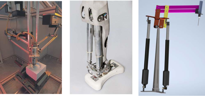
Figure 1: The parallel mechanisms used in different applications. From left: Orthoglide used in milling operations [19], active ankle used in humanoids [24], RCM mechanism used in surgery [12]

In the past, several optimization methods were proposed for mechanism synthesis. Some of them utilize the mathematical formulation of the objective function in order to implement the gradient descent method [25]. Where the objective function is not available in closed form and/or one cannot exploit gradient-based algorithms, numerical approaches and evolutionary algorithms were extensively implemented. Among them, we mention DE [26] and Genetic Algorithms (GA) [27] for single objective optimization and Branch and Prune [28], Interval based analysis [23] and NSGA-II [29, 30, 31, 32] for MOO, in which the theory of genetic evolution is implemented. Other evolutionary algorithms that have been implemented are PSO [33] and MOEA/D, which are claimed to be superior to NSGA-II [34]. In general, the above-mentioned algorithms are computationally expensive, and their efficiency highly depends on the population size. Also, only a guess of the required set of initial population is available for convergence in the global search. The computational time increases considerably with increasing population size and thus limits the application of such methodologies in case of computationally expensive objective functions and also limits the number of constraints that can be implemented.
A recent work in mechanism design optimization is co-optimization with the motion trajectories [35]. In this approach, the design parameters and the motion equations are represented implicitly and efficient algorithms are used to explore the implicitly defined manifold. This type of methodology utilizes all the advantages of expressing the problem as an implicit function, but it is not always possible to do the same.

To reduce the computational cost of optimizing a mechanism, a local search method can be implemented. To avoid the solution converging to a local optimum, different methodologies are employed to combine local optimization methodologies with global searches [36, 37, 38, 39]. Most of the literature presented above focuses primarily upon the problem formulation and use the existing methodology as an optimization tool. A deeper analysis into the implementation of the optimization algorithm for PKM provides more flexibility and capability to handle different constraints efficiently. The geometrical method of proposing the next best solution in Nelder-Mead algorithm is best suited for mechanism optimization as the properties of the mechanisms are influenced by the lengths of the links and the exploration of design space in Nelder-Mead approach is very relevant to convergence to optimized parameters.

In this work, we present a new design optimization methodology that can adapt to constraints involving internal collisions along with the physical joint limits and physical stroke of the actuator and classical criteria such as the condition number or the velocity amplification factor (VAF). We propose a fast local search algorithm, i.e. the Nelder-Mead algorithm, coupled with a global search procedure. A novel method is proposed to the local search by using different initialization in enabling one to compare results from a greater span in the optimization space. This method allows moving towards a global optimum faster, even for mechanisms that have computationally expensive objective functions. The overall output of the work is an accelerated general algorithm for PKM design optimization which is flexible with respect to the definition of the objective function as well as is modular and adaptive to any constraints. Two different PKMs used in different applications are optimized using the proposed method to illustrate the advantage in terms of flexibility of the methodology.

The paper is organized in the following way: Section 2 discusses the objective functions and constraints relevant to PKM design. It highlights the importance of choosing proper constraints for mechanisms with prismatic joint. Section 3 details the optimization methodology that combines local and global searches and illustrates the novelty in accelerating the local search. Section 4 provides the examples for the two PKM design optimization with different objective functions and constraints and their corresponding optimized parameters. In Section 5, some conclusions are presented, along with a few pointers to future work.

2 Design considerations in PKM optimization

In the parallel kinematic mechanism design the following choices have to be made:

1. Architecture of the manipulator (e.g: 3RRR(Revolute-Revolute(actuated)-Revolute), 3RPR(Revolute-Prismatic(actuated)-Revolute) etc.)

2. Type of joints: different combinations of joints to achieve the same dof (e.g: UPS(Universal-Prismatic(actuated)-Spherical), RUS, RRPS)

3. Pose of the joints: where to place and how to place a particular joint’s frame?

Making a particular choice is non-trivial, especially because of its effect on the workspace, the kinematic solutions and the size of the mechanism. Another interesting challenge is that the same architecture can be used to perform different tasks with either kinematic or dynamic constraints, and thus have to be optimized accordingly. The following subsections elaborate on the common objective functions and constraints involved in mechanism optimization to motivate the choice of the algorithm.

2.1 Objective function

It is important to evaluate the quality of the motion performed while designing a manipulator with kinematic characteristics. The quality indices widely used in the past are the conditioning number [20] and the manipulability ellipsoid [21]. The feasible workspace and the global quality of the manipulator are directly related in the presented case, and thus can be implemented together with appropriate weights.

2.1.1 Workspace of the manipulator

This work considers a RDW without singularity which is an n-dimensional sphere in the n-dimensional output space and the center of the workspace is the home configuration (i.e, where all the actuator values are zero). To allow the implementation of the mechanism for multipurpose applications, the required workspace is not treated as a constraint. Instead, the algorithm tries to achieve maximum feasible workspace in the desired RDW ($RDW_{d}$) [23].

In contemporary, the concept of safe working zone for parallel manipulators has been introduced in [40] where a feasible workspace is free of singularities and internal link collisions and satisfies passive joint limits. This work considers only the collision of actuating prismatic joints, as the rest of the links can be redesigned to counter the resulting collision issues, if any. The context of FS in this literature relates to the set of all points in the discretized op_space such that:

1. They are non-singular configurations

2. Respect passive joint limits

3. For any postures, there is no internal collision between the actuators and the moving platform

2.1.2 Quality of the manipulator

The cnum was introduced in [20] to quantify the quality of motion. It is defined as the value of the asymptotic worst-case relative change in the output for a relative change in the input, and is used to measure how sensitive the output is to changes in the input. The geometrical interpretation of cnum is the quantity proportional to the eccentricity of the ellipsoid, giving information about the ease of travel in a particular direction from a current end effector pose. When the cnum is equal to 1, we have a sphere, and it corresponds to the isotropic configuration. The value of cnum ranges from 1 to $\infty$ and so its inverse, $\kappa^{-1}$, is used for bounded values and is given by (1), where $\sigma$ are the singular values of the Jacobian matrix, $\mathbf{J}$.

$$\kappa^{-1}=\dfrac{\sigma_{min}}{\sigma_{max}},\hskip 8.53581pt\kappa^{-1}\in[0,1]$$ (1)

The conditioning number suffers from dimensional non-homogeneity of the Jacobian matrix and is not suitable for manipulators with both translational and rotational movements [41]. This is an important issue to consider while implementing the proposed optimization methodology for a general manipulator. The manipulators presented in Section 4 have only rotational, dof and so the inverse of the conditioning number is chosen as the quality index. A gqi (GCI), the mean of summation of the values of qi over the regular dextrous workspace, is defined as follows,

$$\kappa^{-1}_{g}:=\dfrac{\sum\limits_{1}^{RDW_{d}}\kappa^{-1}}{RDW_{d}}$$ (2)

2.2 Constraints

Parallel Kinematic Manipulators (PKMs) have three distinct features from a serial chain:

1. singularity inside the workspace where the control of the end-effector is lost;

2. passive joints whose orientation can be calculated but not controlled explicitly;

3. multiple legs - serial chains connecting the end-effector with the base.

These three features are of great importance as they affect the workspace of the manipulator as well as the nature of the motion. So, we take note that the passive joint limits and avoiding internal collisions among different legs of the PKM are two important constraints to be implemented in our optimization problem.

2.2.1 Non-singular constraint

The discretized output space (op_space) of the parallel mechanism is separated by the singularity surfaces, thus resulting into several connected regions also called aspects [42]. As it is not possible to travel from one aspect to another, it is important that the desired RDW ($RDW_{d}$) lies in a single aspect. As an example, Figure 2 represents the output space for a mechanism with 2 orientation dofs and the black circle is the desired workspace. Figure 2(left) illustrates a valid set of parameters whereas figure 2(right) corresponds to a non-valid architecture of the mechanism because it consists of multiple connected regions, then there are multiple aspects, and thus we cannot travel to every configuration in the RDW.

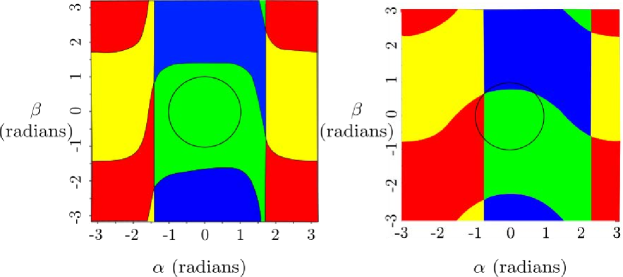
Figure 2: The aspects in the workspace with different parameters for the 2UPS-1U mechanism from [12, 43]

2.2.2 Passive joints

The architecture of PKM is such that there are multiple passive joints in each leg. These passive joints are of prime importance in deciding the nature of the degree of freedom as well as the singular configuration. The joint positions as well as their limits are critical for the analysis. The passive joints can be either prismatic, revolute or a higher pair of joints. It is considerably easy to specify the limits in case of prismatic or revolute joint, but it may not be easy when we use a universal joint or a spherical joint. Implementing passive joint limits in the optimization process allows achieving a practical result for the design and gives more clarity about the feasible workspace.

2.2.3 Link collisions

As PKM consists of multiple serial chains attached to the end effector from the base, internal collisions are an important aspect of workspace analysis and synthesis as they strongly affect the workspace and other kinematic properties. The theoretical workspace is generally different from the practical realization, because of the mechanical joint limits and link collisions in the mechanism [44]. Analysis of such self collisions is critical in parallel manipulators. The implementation of link collisions as a constraint is even more complicated since it depends not only on the architecture of the serial legs but also on the design of the links as well as their assembly. Different approaches have been used to calculate the collision between the links. The work reported in [45, 46] uses a common normal to determine the distances between two links, while a more modern approach is to use Computer Aided Design (CAD) [47, 48]. The presented work only considers the collision between the actuators, and thus the method suggested in [45, 46] suffices.

2.2.4 Feasible actuator range: constraint for mechanisms with prismatic actuators

Another important constraint while designing a PKM is the active joint ranges. This constraint is specifically relevant to the mechanisms with prismatic joints as actuators. The aim is to implement a constraint on the actuators to be chosen in order to maximize the points in $\mathcal{F}\bigcap RDW_{d}$. Generally, a prismatic joint is expressed as a constraint with a certain minimum and maximum range and with a constraint on the ratio between the length in completely actuated state and its default length:

$$\rho_{min}\leq\rho\leq\rho_{max}$$ (3)

$$\rho_{max}\leq\text{stroke}\cdot\rho_{min},\hskip 8.53581ptstroke\in[1,2]$$ (4)

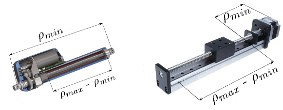
Figure 3: The industrial prismatic joints and the relation between $\rho_{min}$ and $\rho_{max}$. Source: Hanpose linear actuator HPV5 SFU1204, www.pngegg.com/en/png-mckkp.

Equation 4 comes from the physical structure of general prismatic joints. If the unextended length of the actuator is $\rho_{min}$, then it is not practical for common prismatic joints to extend beyond their original length ($\rho_{max}<2\cdot\rho_{min}$) as explained in figure 3. The novelty in expression of the actuator range in the present work is that we do not have a static value as a limit as mentioned in Equation 3, i.e, we express the constraint only in terms of the stroke ratio defined in Equation 4. This allows us to choose the best actuator ranges to maximize the feasible workspace without putting any constraint on the minimum or maximum size of the prismatic joint. This is illustrated in figures 4 and 5 which introduce an example for a 2 dof 2UPS-1U orientation mechanism from [12]. The points in the dotted space in figure 4 are pairs of values corresponding to the actuator lengths in a feasible configuration. The aim is to search for an optimized bracket, [$\rho_{min},\rho_{max}$], i.e, a bracket that includes as many blue points as possible with the constraint that the side of the square does not exceed a given proportion with respect to its minimum value.

The algorithm 1 explains the method used to get the optimized bracket for the actuators. After discretizing the $RDW_{d}$, we get the set of all valid points belonging to $\mathcal{F}$. Upon calculating the values for actuator length at each point, the minimum $\rho_{min}$ and maximum $\rho_{max}$ value for the actuator is obtained. The input of the algorithm is a n x 3 matrix for the n valid points, with columns corresponding to the actuator lengths and the evaluation at that point. If the ratio of maximum value to minimum value of the actuator length respects the stroke ratio, then the algorithm returns the actuator range without alteration. Otherwise, a bracket of [$\rho_{min}$, stroke.$\rho_{min}$] is generated and the values of the actuator lengths for each point in the set of valid points is checked against the bracket and the number of points satisfying the bracket is stored. This process is repeated by incrementing the $\rho_{min}$ till the value of stroke.$\rho_{min}$ is lower than $\rho_{max}$. The algorithm returns the optimized actuator lengths along with the corresponding evaluation of the objective function for given parameters.

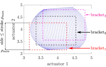
Figure 4: Different search brackets within the actuator space (ip_space). The dots correspond to the pair of lengths of actuators for a configuration in RDW.

(a) Feasible workspace (white) when bracket 1 in figure 4 is implemented

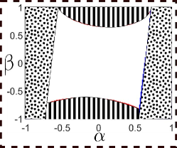
(b) Feasible workspace (white) when bracket 2 in figure 4 is implemented

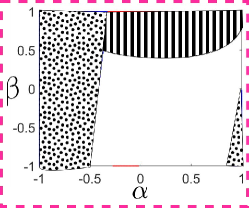
(c) Feasible workspace (white), bracket 3 in figure4 is implemented

Figure 5: Comparison of feasible workspace (white space) within the $RDW_{d}$ for different search brackets and a specific mechanism (2UPS-1U). The striped and dotted part represent the violation due to actuator lengths of first and second leg, respectively.

Result: evaluation, e, and corresponding range of actuators, $\mathbf{\rho_{range}}$

1 $\mathbf{input}$ $\rightarrow$ $\mathbf{valid\_points}$ that satisfy all the constraints;

2 $\mathbf{\rho_{range}}$ = [min($\mathbf{\rho_{vec}}$), max($\mathbf{\rho_{vec}}$)] = [$\rho_{min}$, $\rho_{max}$];

3 stroke : The maximum allowable stroke ratio, see Eq. (4);

4 steps : number of brackets used (see figure 4);

5

6 Checking for feasible set of the actuators;

7 if $\rho_{max}\geq stroke\cdot\rho_{min}$ then

8       for $\rho_{lower}$ from $\rho_{min}$ to $\dfrac{\rho_{max}}{stroke}$ by steps do

9             e = 0;

10             for n from $1$ to length($\mathbf{valid\_points}$) do

11                   if $\rho_{1},\rho_{2}\geq\rho_{lower}$ and $\rho_{1},\rho_{2}\leq$ stroke$\cdot\rho_{lower}$ then

12                         j = j+1 $\triangleright$ Incrementing the number of feasible points;

13                         e = e + $\mathbf{valid\_points}$[n, 3];

14                        

15                   end if

16                  

17             end for

18            $\mathbf{eval\_vector}$[k]= [e, $\rho_{min}$, j];

19             k = k + 1;

20            

21       end for

22      [$e_{1}$, $\rho_{min}$, $i_{1}$] = max($\mathbf{eval\_vector}$, 1);

23       e = $\mathbf{eval\_vector}$[$i_{1}$][1];

24       $\rho_{min}$ = $\mathbf{eval\_vector}$[$i_{1}$][2];

25       $\mathbf{\rho_{range}}$ = [$\rho_{min}$, stroke.$\rho_{min}$];

26      

27      

28else

29      e = max($\mathbf{valid\_points}$[3]);

30       $\mathbf{\rho_{range}}$ = [min($\mathbf{\rho_{vec}}$), max($\mathbf{\rho_{vec}}$)]

31 end if

return $e$, $\mathbf{\rho_{range}}$

Algorithm 1 Implementation for choosing the best actuator range

2.2.5 Implementation of constraints and evaluation function

Algorithm 2 illustrates the methodology used to evaluate a given set of parameters. The optimization space is discretized, and each point is evaluated for the constraints. Some constraints are implemented strictly, in the sense that if even one point in the $RDW_{d}$ violates the constraint, then we discard the given set of parameters as an invalid solution. The singularity constraint is a strict constraint in the present algorithm, in the sense that if the singularity curve intersects with even one point of $RDW_{d}$, the evaluation for given parameters is negative. In cases where the $RDW_{d}$ is singularity free, if all other constraints (e.g: passive joint limits, collision constraints) are satisfied at a particular point in the $RDW_{d}$ then it is rewarded by the corresponding $\kappa^{-1}$ value or if there is a violation of these constraints (except singularity) the point in $RDW_{d}$ is given 0 value. As we examine each point in the discretized workspace, the final evaluation is the cumulative value of $\kappa^{-1}$ over the workspace where all the constraints are satisfied. The rewarding strategy can be changed as per the designer’s needs, and desirable weightage can be assigned to the constraints to achieve an optimized design for a specific requirement.
The modularity of the algorithm with the constraints can also be observed in Algorithm 2. It can be seen that the constraints are completely independent of each other, allowing to activate, deactivate any constraint or add other constraints without requiring any change to the algorithm. This is especially useful for mechanism design, as it provides flexibility to experiment the effect of different constraints on the final feasible workspace. As each constraint can be designed individually to reward or penalize a particular set of parameters, the designer can have a blend of strict and non-strict constraints in the optimization. The designer can also identify which constraint stops the optimization and needs to be modified.

Result: evaluation at a given point in optimization space and the corresponding actuator lengths

1 $\mathbf{input}$ $\rightarrow$ $\mathbf{v}$ $\triangleright$ It is a n-dimension point in given n-dimension optimization space;

2 $x_{i},i\in{1,..,n}$, $\triangleright$ $i^{th}$ variable of the n-dimension optimization space;

3 $\rho_{1}$ and $\rho_{2}$ $\triangleright$ actuator lengths at a given configuration;

4 e = 0 $\triangleright$ Initialising the evaluation;

5 for $x_{1}$ from $x_{1min}$ to $x_{1max}$ by $interval_{i}$ do

6       … $\triangleright$ Add loops as a function of the dimension of the space

7       for $x_{n}$ from $x_{nmin}$ to $x_{nmax}$ by $interval_{n}$ do

8             f($\mathbf{v}$) $\triangleright$ function that solves IGS, collision distance and $\kappa^{-1}$;

9             [det($\mathbf{J}$), $\mathbf{q}_{p}$,  $\rho_{1}$,  $\rho_{2}$,  $\kappa^{-1}$, $d_{c}$] = f($\mathbf{v}$);

10             f($\mathbf{v}$) returns the value of the determinant of Jacobian, the passive joint angle vector, $\mathbf{q}_{p}$, actuator lengths, [$\mathbf{\rho}_{1},\mathbf{\rho}_{2}$], the inverse of the conditioning number, $\kappa^{-1}$ and the collision distance, $d_{c}$, between the actuators;

11            

12             $\triangleright$ 1. Checking for singularity constraints;

13             if det$(\mathbf{J})$ is 0 then

14                  e = -$\infty$;

15                   break;

16            else

17                  $reward$ = $\kappa^{-1}$

18             end if

19            

20             $\triangleright$ 2. Checking the passive joint limits;

21             for i from 1 to length of $\mathbf{q}_{p}$ do

22                  if $q_{pi}\geq q_{pmax}$ or $q_{pi}\leq q_{pmin}$  then

23                        $reward=0$

24                  else

25                        $reward$ = $\kappa^{-1}$

26                   end if

27                  

28             end for

29            

30             $\triangleright$ 3. Checking for collision constraints;

31             if $d_{c}\geq$ threshold then

32                  $reward$ = 0

33             end if

34            e = e + reward;

35             $\mathbf{valid\_points}$[i] = [$\rho_{1}$, $\rho_{2}$, reward];

36            

37       end for

38      …

39      

40 end for

41Implement the algorithm 1;

return $\mathbf{valid\_points},e,\mathbf{\rho}_{1},\mathbf{\rho}_{2}$

Algorithm 2 Method to calculate the evaluation and $\mathbf{\rho}_{range}$ for a set of parameters

3 Proposed Algorithm for Mechanism Optimization

In this section, the complete optimization methodology is illustrated. Recalling from the previous sections, the aim is to implement an algorithm that is capable of handling the non-smooth objective functions as well as the constraints related to PKM design. This section is divided in three subsections detailing the local search, the global search and the strategy used to couple them both for faster and more efficient solutions, respectively.

3.1 Local search algorithm: The Nelder-Mead (NM) algorithm

The Nelder-Mead algorithm is a derivative-free optimization algorithm proposed by John Nelder and Roger Mead [49]. It is also called the downhill-simplex algorithm, as it uses simplexes to search the space locally. In this section, we present the algorithm for a single start, which searches for the optimum solution in the local vicinity of the initial simplex. Later, we discuss the implementation of the algorithm in mechanism optimization and detail the method for extracting the best actuator ranges from the solution. The section is concluded with a summary of the algorithm and its implementation, highlighting few strengths and weaknesses of the same.

For a n-dimensional o_space, we require a simplex of at least n+1 points in o_space to avoid premature convergence. This can be explained with a simple graphics for 2-dimensional, o_space as show in figure 6.

(a) Example mapping with 2 optimization variables.

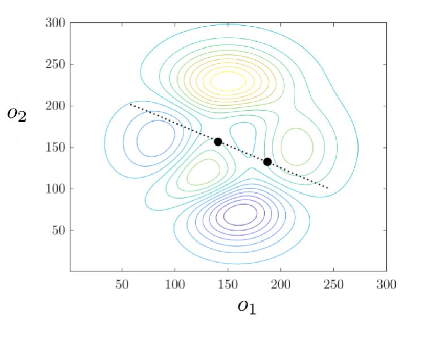
(b) The traversing in $\mathcal{O}$-space with 2 point simplex, we can explore the points on the line only

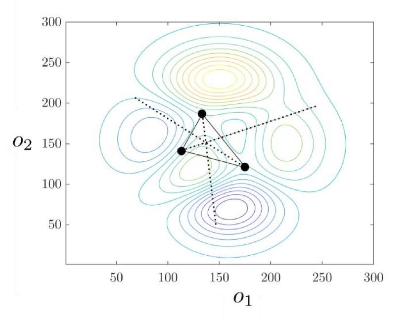
(c) The traversing in $\mathcal{O}$-space with 3 point simplex, allowing to explore the complete space

Figure 6: Premature convergence when using a simplex of less than (n+1) points in n-dimensional $\mathcal{O}$-space. The example is taken from Matlab function [X, Y, Z] = peaks(25), MATLAB 2021

The algorithm is initiated with a sorted simplex of n+1 points ($\mathbf{v_{0}},\mathbf{v_{1}},...\mathbf{v_{n}}$) such that the objective function evaluated of the $i^{th}$ vertex has a value better than or equal to that of the $(i+1)^{th}$ vertex. A mean point ($\mathbf{v_{m}}$) is calculated by excluding the worst point ($\mathbf{v_{n}}$):

$$\mathbf{v_{m}}:=\dfrac{\sum\limits_{i=0}^{n-1}\mathbf{v_{i}}}{n}$$ (5)

The optimization algorithm then compares the mean point and searches for better points by geometrical operations termed as (i) reflection, (ii) expansion, (iii) inside contraction, (iv) outside contraction and (v) shrinkage. These operations are defined as follows:

1. Reflection ($\mathbf{v_{r}}$) :

   $$\mathbf{v_{r}}=\mathbf{v_{m}}+r\,(\mathbf{v_{m}}-\mathbf{v_{n}}),\hskip 8.53581ptr=\text{reflection coefficient}\,(r>0)$$ (6)

2. Expansion ($\mathbf{v_{e}}$) :

   $$\mathbf{v_{e}}=\mathbf{v_{m}}+e\,\mathbf{(v_{r}-v_{m})},\hskip 8.53581pte=\text{expansion coefficient}\,(e>1)$$ (7)

3. Outside contraction ($\mathbf{v_{oc}}$) :

   $$\mathbf{v_{oc}}=\mathbf{v_{m}}+k\,(\mathbf{v_{m}}-\mathbf{v_{n}}),\hskip 8.53581ptk=\text{contraction coefficient}\,(0<k<r)$$ (8)

4. Inside contraction ($\mathbf{v_{ic}}$):

   $$\mathbf{v_{ic}}=\mathbf{v_{m}}-k\,(\mathbf{v_{m}}-\mathbf{v_{n}}),\hskip 8.53581ptk=\text{contraction coefficient}$$ (9)

5. Shrinkage:

   $$\forall\,i\in[1,n]\hskip 8.53581pt\mathbf{v_{i}}=s\,.\mathbf{v_{i}},\hskip 8.53581pts:=\text{shrinkage factor}\,(0<s<1)$$ (10)

The new point ($\mathbf{v_{n}}$) introduced in the simplex depends on the evaluation of the $\mathbf{v_{r}}$, $\mathbf{v_{e}}$, $\mathbf{v_{oc}}$ and $\mathbf{v_{ic}}$ (see Algorithm 4). The operation is continued until the stopping criteria are reached. The simplex stops if it shrinks below a certain value, $\epsilon_{1}$ and the evaluations of every vertex of the shrunk simplex vary by a maximum threshold $\epsilon_{2}$. The algorithm can be stopped by limiting the number of iterations, too. The stopping criteria was presented in Algorithm 3 and the complete procedure for one start of the NM-algorithm is given in Algorithm 4. An example of the operations in a 2-dimension optimization space, o_space, is illustrated in figure 7(a) to present the geometric nature of search of the o_space in NM-algorithm. In figure 7(b), an example of the points explored during an optimization process is graphically represented.

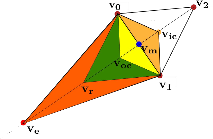
(a) An example of an operation on a simplex (defined by $v_{0},v_{1},v_{2}$) in 2-dimensional $\mathcal{O}$

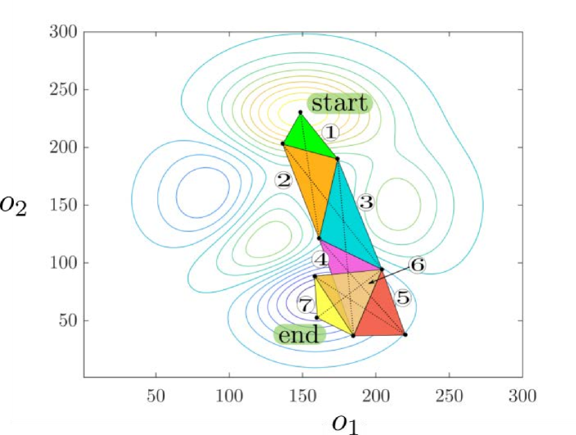
(b) An example of the travel path of optimization in Nelder-Mead algorithm on the contour plot of peaks(25) function

Figure 7: The single start of the Nelder-Mead local search

Result: Boolean for stopping condition

1 sorted simplex $\{\mathbf{v_{0}},\mathbf{v_{1}},\mathbf{v_{2}},...,\mathbf{v_{n-1}},\mathbf{v_{n}}\}$;

2 evaluations {$e_{0},e_{1},e_{2},...,e_{n-1},e_{n}$};

3 maximum iteration = max_iter… from algorithm 4;

4 iteration count = iter;

5 $l_{ij}$ = $\left\lVert\mathbf{v_{j}}-\mathbf{v_{i}}\right\rVert$… length of the side of simplex;

6 $e_{ij}$ = $|$$e_{i}$ - $e_{j}$$|$;

7 if max($l_{ij}$) $\leq\epsilon_{1}$ $\&\&$ max($e_{ij}$) $\leq\epsilon_{2}$ then

8      stop = 1

9      break

10 end if

11if iter $\geq$ max_iter then

12      stop = 1

13else

14      stop = 0

15 end if

Algorithm 3 Stopping criteria for the NM algorithm

Result: Local minimum evaluation and the optimized parameters

1 initial sorted simplex $\{\mathbf{v_{0}},\mathbf{v_{1}},\mathbf{v_{2}},...,\mathbf{v_{n-1}},\mathbf{v_{n}}\}$;

2 evaluations $\{e_{0},e_{1},e_{2},...,e_{n-1},e_{n}\}$;

3

4while stop = 0  do

5       calculate $\mathbf{v_{m},v_{r}}$ and $e_{r}$;

6       if ($e_{n}<e_{r}<e_{0}$) then

7             $\mathbf{v_{n}}$ = $\mathbf{v_{r}}$;

8            

9       else if ($e_{0}<e_{r}$) then

10             if ($e_{r}<e_{e}$) then

11                  $\mathbf{v_{n}}$ = $\mathbf{v_{e}}$;

12            else

13                  $\mathbf{v_{n}}$ = $\mathbf{v_{r}}$;

14             end if

15            

16      

17      else if ($e_{n}<e_{r}<e_{n-1}$) then

18             if ($e_{oc}>e_{r}$) then

19                  $\mathbf{v_{n}}$ = $\mathbf{v_{oc}}$;

20                  

21            else

22                  $\forall\,i\in[1,n]\hskip 8.53581pt\mathbf{v_{i}}=s.\mathbf{v_{i}}$;

23             end if

24            

25      

26      else if ($e_{r}>e_{n}$) then

27             if ($e_{ic}>e_{r}$) then

28                  $\mathbf{v_{n}}$ = $\mathbf{v_{ic}}$;

29            else

30                  $\forall\,i\in[1,n]\hskip 8.53581pt\mathbf{v_{i}}=s.\mathbf{v_{i}}$;

31             end if

32            

33       sort the simplex;

34       if $\mathbf{v_{0new}}>\mathbf{v_{0}}$ then

35            iter = 0

36      else

37            iter = iter + 1

38       end if

39      Update ’stop’ from Algorithm 3

40 end while

return $\mathbf{v_{0}},e_{0}$

Algorithm 4 Single start of the Nelder-Mead optimization algorithm

3.1.1 Pros and cons of the NM-algorithm

The Nelder-Mead algorithm is quite straightforward to model the optimization problem for mechanism design. This allows us to design a general methodology for optimizing any parallel mechanism. As it is a derivative-free algorithm, we can introduce complex objective functions that are hard to formalize. An example is the quality index, gqi, defined in Section 2.2. Also, as NM-algorithm is a local search algorithm, it returns a stationary point in a considerably low time compared to the currently implemented global optimization methodologies. This makes it possible for the designer to structure an objective function that is computationally expensive. Also, the constraints can be constructed in modular way, allowing to experiment with different constraints at any stage of the development. Another important advantage of the Nelder-Mead algorithm relevant to the mechanism design is its geometric search method. The basis of optimization space in NM-algorithm is the optimization variables themselves. It is logical to use this method because the next best design parameters are chosen as a result of the combination of parameters of previous simplex, rather than using complex methods to represent a mechanism in the optimization space which may not have geometrical explanation for choosing the next best proposal (e.g: chromosomes in Genetic Algorithm). We can also tune the exploring parameters, i.e., the reflection, expansion, contraction and shrinkage coefficients, with human intuition and some prior knowledge about the importance of different parameters.

Though suitable for our application, there are certain disadvantages of using the NM algorithm, too. Under some hypotheses, the algorithm has proof of convergence up to dimension 2 [50] and has no proof for convergence beyond 2-dimensional optimization. If not implemented correctly, it gets into a collapsing simplex patterns, thus converging to a non-stationary solution [51]. The convergence highly depends on the initial size of the simplex and the choice of the coefficients, as discussed in [52]. Despite these shortcomings, the NM-algorithm is useful in our case as the aim is not finding the absolute optimized design parameter but to satisfy all constraints and then get an acceptable quality of performance. Indeed, it has been implemented in various applications with great success [38, 39]. Different convergent variants have also been proposed to get around the premature convergence [53], allowing the algorithm to explore extra points in case of near collapse.

To get better results, local search of the NM algorithm is complemented with a multi-start technique for a global search in the optimization space, as discussed in the next section.

3.2 Global search algorithm

The NM algorithm combined with other global search methods such as low-discrepancy points [54], genetic algorithm [36] and Powell optimization [37] have been proposed in the past. We implement a multi-start Nelder Mead algorithm with low discrepancy points [55, 56, 57] for exploring a global optimization space. In this method, we execute the NM algorithm with different initial simplexes. It is very important to have a uniformly distributed initial simplexes over the optimization space, in order to explore the maximum area of the optimization space.

3.2.1 Initial simplexes for multi-start

An easily implementable way to obtain a sampling set $\mathcal{O}_{M}\subset\mathcal{O}$ is Monte Carlo sampling with a uniform distribution (see, e.g., [58]), i.e., random sampling. Unfortunately, it is known [56] that the resulting points have the tendency to form clusters, particularly in high-dimensional contexts, which undermine the uniformity of the discretization. A better choice consists in having the $\,M$ points of the discretization $\,\mathcal{O}_{M}$ of $\,\mathcal{O}$ spread “well-uniformly”. In particular, it is desirable that the points be close enough to one another, without leaving space regions under sampled. To this end, as done in [57, 59], one can use certain deterministic sampling techniques. The properties of such techniques are detailed in [57]. The work in [57] suggests that an efficient way of generating uniformly scattered deterministic sets of points consists in taking finite portions of so-called low-discrepancy sequences such as the Halton sequence, the Hammersley sequence and the Sobol sequence. The reported work utilizes initial simplexes chosen from the Sobol sequences, as they prove to be more uniformly distributed.

Figure 8 from [59] shows the comparison between a sampling of the 2-dimensional unit cube by a sequence of 500 points i.i.d. according to the uniform distribution and by a sampling of the same cube obtained via a low-discrepancy sequence (in this case, the Sobol sequence [60]). It can be clearly seen how the space is better covered by the second sequence, as well as how the largest empty spaces among the points appear in the first sampling scheme.

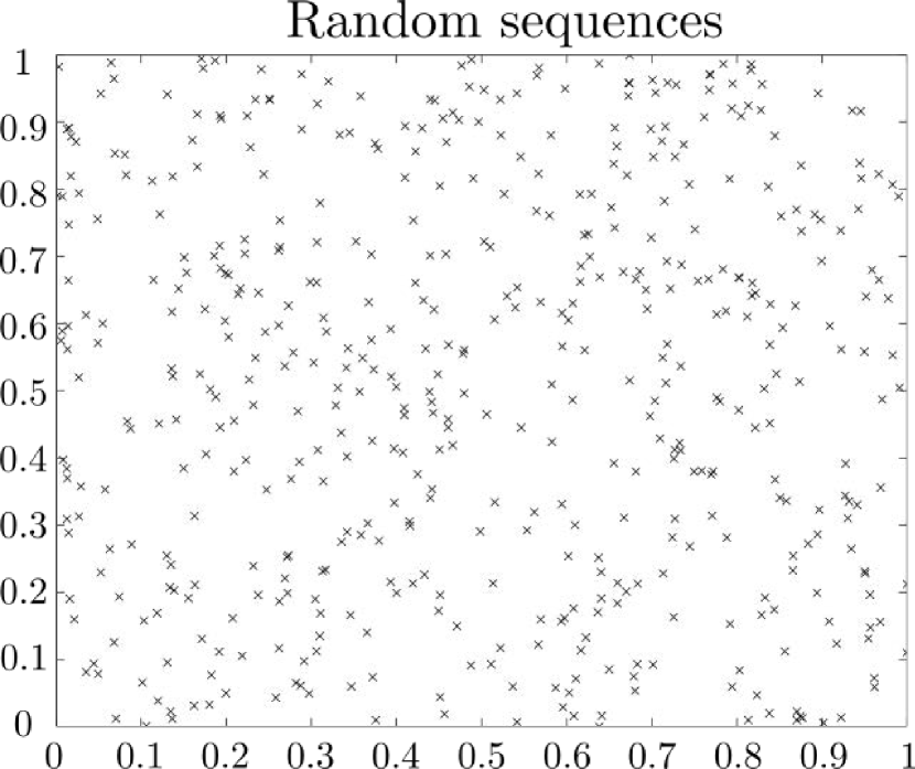
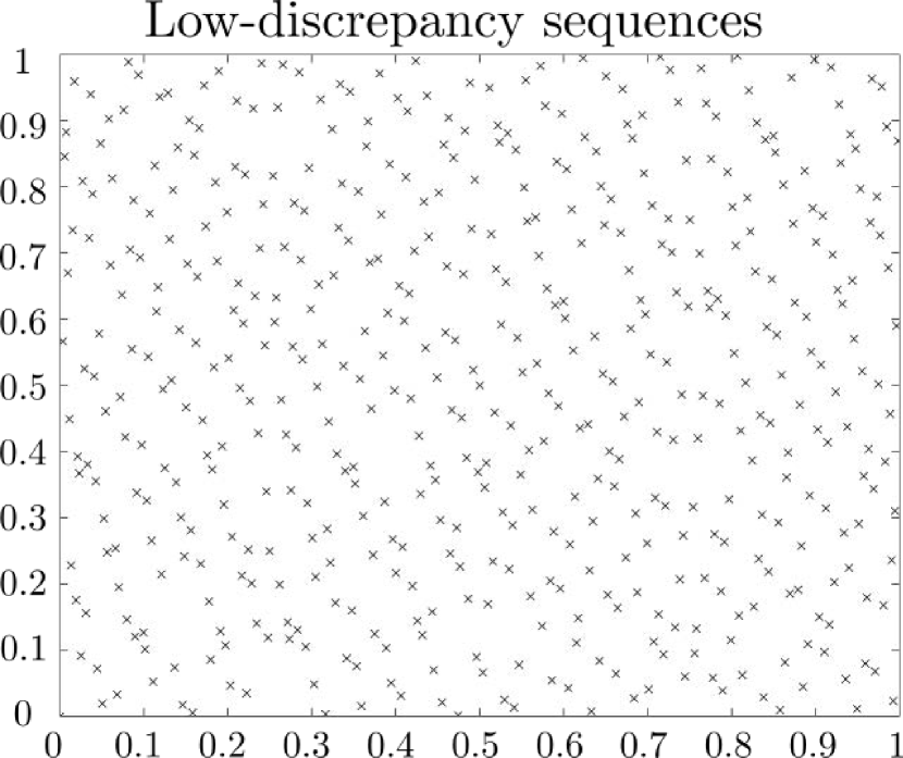
Figure 8: Comparison between random and low-discrepancy sampling of the unit square [59]

3.3 Cascade optimization

In a normal execution of the Nelder-Mead algorithm, the iteration stops either when the simplex has shrunk to a desirable size with near the same evaluations or if we have encountered the same best point for preset allowable maximum iterations, refer to Algorithm 3. In an attempt to decrease the time for local convergence, allowing us to explore more initial simplexes, we adapt a methodology inspired from the practice of rough and fine turning in lathe machines. In general, when we want to remove the excess stock from the workpiece as rapidly as possible, we increase the feed rate and do not focus on the finish of the work. Later, when we are close to desired dimensions, the feed is decreased and now the focus is shifted on the finishing of the work. Figure 9 illustrates the complete flow of the algorithm. In the beginning, the simplexes taken from the Sobol sequence are initialized in multi-start NM-algorithm and a coarse search is performed for the local optima. Later, the local optima from some chosen initialized simplexes are used to implement stricter stopping criteria, allowing them to converge to a stationary point with finer quality. Fundamentally, we are discarding the local optima that do not promise a good evaluation even after a longer search, decreasing the computational time considerably. Also, as we already have an optimized vertex as an initial simplex, we can build the rest of the vertices as per our choice, thus controlling the size of the initial simplex.

3.3.1 Coarse search

In the coarse search, we want to accelerate the local convergence, allowing us to maximize the number of starts in our optimization methodology. This is done by using a coarser search space and relaxing the stopping criteria. In the coarse search, the output space is discretized with an interval 10 times larger than in the finer search. This drastically brings down computational time. The aim of the coarse search is to find the simplexes that lie on relatively steeper slopes in the optimization space. By relaxing the stopping criteria, the maximum iterations allowed to repeat with the same evaluation is capped at 10 which helps in terminating the local search faster. One of such coarse implementation is detailed in Algorithm 5, where the condition of incrementing the iteration is changed. We implement a condition that the new evaluation found is better than the previous only if it exceeds the previous evaluation by 5% and the algorithm stops as soon as we have 90% of the maximum expected value.

Unlike other optimization problems, in the PKM design the maximum optimized evaluation is known. For example, if we are discretizing the output space in 1000 points and are rewarding a value of 1 for a feasible point and 0 for infeasible points, then the maximum evaluation of such rewarding strategy is 1000. This fact is so useful that we can now have criteria related to the maximum expectation and the current evaluation. In the coarse search, we implement a constraint such that if an evaluation is greater than 80% of the maximum evaluation, then terminate the iterations. This particular methodology lowers the optimization time drastically when the constraints are not too strict, and we have many parameters satisfying the constraints. It is interesting to note that this methodology can be used irrespective of the rewarding strategy.

3.3.2 Fine search

In the fine search, we filter the different local optima obtained from the coarse search. The evaluations of the local optima are arranged in increasing order, and the top 10% of the collected optima are chosen for further evaluation. In the fine search, we implement stricter stopping criteria, change the constraint of maximum expected evaluation to 100% and discretize the output space with a 10 times finer interval. The margin that is considered as an improvement is lowered to 1%. These changes directly affect the computational time and take much longer time with increasing dimension of the output space. All the optimized parameter sets from the NM-algorithm with finer constraints are compared, and the best point is proposed as an optimized parameter of the PKM.

Result: Optimised parameter set $\mathbf{v_{0}}$

1 input : Initial set of simplexes;

2 $e_{0}$ : the best evaluation from the previous iteration;

3 $e_{max}$ : Maximum expected evaluation;

4 limit : The percentage of maximum evaluation that is considered best;

5 For coarse search;

6 max_iter = 3 n;

7 margin = 1.05 … (suggesting $\geq$5% increment is considered improvement);

8 limit = 0.8 … (suggesting that 80% of maximum evaluation is a criterion to stop);

9 For fine search;

10 max_iter = 10 n;

11 margin = 1.01 … (suggesting $\geq$1% increment is considered improvement);

12 limit = 1;

13 stop = 0;

14 while stop = 0 do

15       Perform algorithm 4 except for last step of checking stop from algorithm 3;

16       Perform algorithm 2 with finer intervals;

17       if $e_{new}$ $\geq$ margin$\times e_{0}$ then

18            iter = 0

19      else

20            iter = iter + 1

21       end if

22      if iter $\geq$ max_iter then

23            return stop = 1;

24       end if

25      if $e_{new}\geq$ limit$\times e_{max}$ then

26            return stop = 1;

27       end if

28      

29 end while

return $\mathbf{v_{0}}$ from the algorithm 4

Algorithm 5 Implementation of coarse and fine local search criteria

Figure 9: The flowchart for the complete implemented optimization methodology

Result: Optimized parameter set of the mechanism and its evaluation

1 Assuming we have ‘m’ starts for a ‘n’ dimensional optimization problem;

2 Choose m.(n+1) valid n-dimensional points from the Sobol set generated;

3 Choose ‘k’ local optima for further fine search, generally, k $\leq$ 0.1 m;

4 for start = 1:m do

5       Initial simplex = $\{\mathbf{v_{(m-1).(n+1)}}...\mathbf{v_{mn+m-1}}\}$;

6       Implement Single start from Algorithm 4 with coarse search from Algorithm 5;

7       $\mathbf{v}_{chosen}(start,1:n+1)=[\mathbf{v}_{0},e_{0}]$;

8      

9 end for

10sort $\mathbf{v}_{chosen}$ by evaluation of the corresponding parameter set;

11 for fine_start = 1:k do

12       Generate n more parameter sets around $\mathbf{v}_{chosen}$(fine_start);

13       Implement Single start from Algorithm 4 with fine search from Algorithm 5;

14       $\mathbf{v}_{fine}$(fine_start, 1:n+1) = $[\mathbf{v}_{0},e_{0}]$;

15      

16 end for

17sort $\mathbf{v}_{fine}$ by evaluation of the corresponding parameter set;

return $\mathbf{v}_{fine}[1,1:n]$, $\mathbf{v}_{fine}[n+1]$

Algorithm 6 An example of implemented multi-start optimization

4 Results and discussion

The optimization algorithm detailed in the work was used to optimize two different parallel mechanisms to validate the general implementation. The mechanisms chosen for optimization are widely used in the industry, and the relevance of the objective function chosen is also detailed in this section. An open source implementation of the proposed algorithm and the examples are available at: https://github.com/salunkhedurgesh/ParaOpt.

4.1 1 dof lambda mechanism

The lambda mechanism is a single closed loop (1-RRPR) mechanism and is used in the legged robots as an abstraction of revolute joint [7, 61, 62] as shown in figure 10. This mechanism is used for a stiffer actuation where a compact, but powerful force is required, and non-linear transmission characteristics are desirable. The constraint equations are straightforward in this case and have been extensively discussed in [63]. The mechanism was optimized by using the value of the determinant of the Jacobian matrix which is a scalar for the given case, $j$, as the GCI and a modified VAF. For the lengths and variables shown in figure 10, the calculations these measures are:

$$\rho^{2} =l_{1}^{2}+l_{2}^{2}-2l_{1}l_{2}\cos(\theta)$$

$$j =l_{1}l_{2}\dfrac{\sin(\theta)}{\rho}$$

$$\text{GCI}_{i} =j$$

$$\text{VAF}_{i} \begin{matrix}\left.\begin{aligned} &=\dfrac{1}{1+\sqrt{2}(\textit{j}-1)^{2}}\\ &=0\end{aligned}\right\}&\begin{matrix}\text{VAF}_{min}<j<\text{VAF}_{max}\\ \text{otherwise}\end{matrix}\end{matrix}$$

GCI $$=\dfrac{\sum\limits_{i=1}^{n}\text{GCI}_{i}}{n}$$

VAF $$=\dfrac{\sum\limits_{i=1}^{n}\text{VAF}_{i}}{n}$$

Parameters	Value	Parameters	Value
optimization dimension	1	Range of parameter	[1, 4]
Number of starts	100	Number of iterations	10
Objective choice	Workspace, GCI, VAF	Velocity amplification range	[0.3, 3]
Workspace ($\theta_{1}$ range)	$45^{0}$ to $135^{0}$	stroke ratio	1.5

Table 1: The parameters set for the optimization of 1-dof lambda mechanism

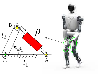
Figure 10: 1-dof lambda mechanism with real life implementation

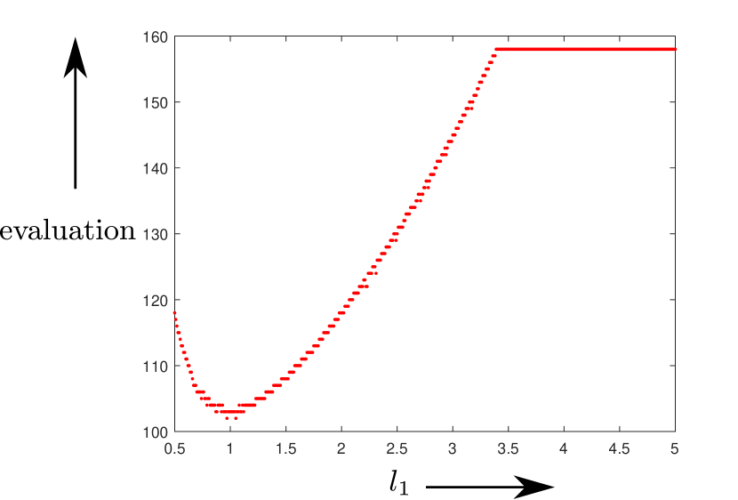
(a) Evaluation of the objective function with varying parameter range(higher the better)

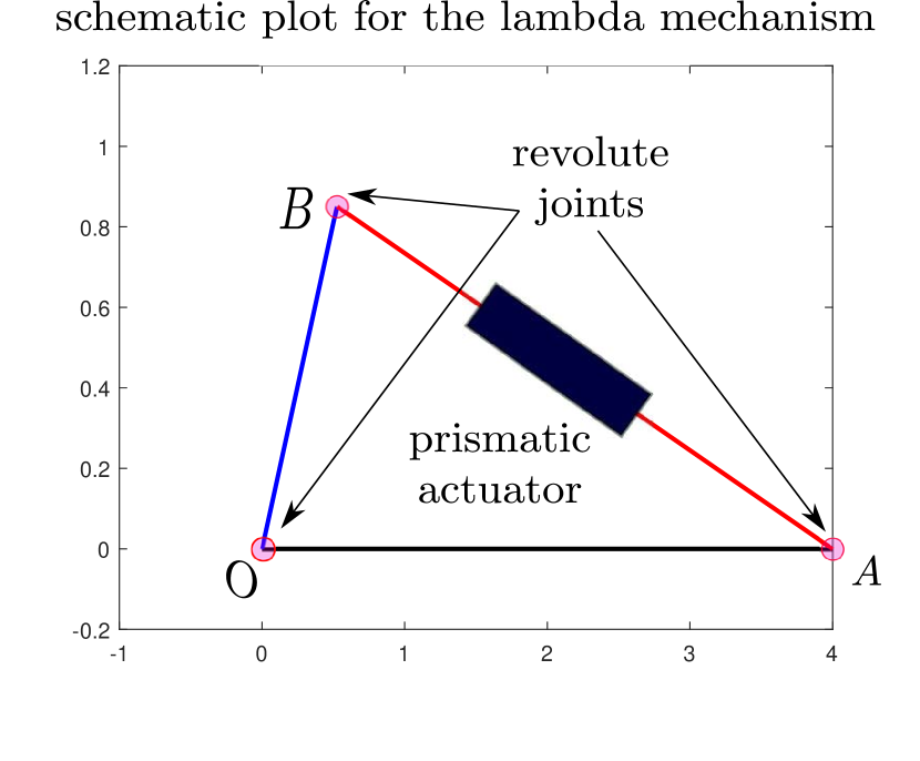
(b) The schematic diagram of optimized lambda mechanism

Figure 11: Evaluation function plot and the schematics of the lambda mechanism for optimized length

In this mechanism, the length of $l_{1}$(OA) is optimized with respect to $l_{2}$(OB) and 3 different objective functions were used with parameters given in Table 1. In the first attempt, the workspace was maximized in order to find a good length such as to cover the revolute joint’s travel from $45^{0}$ to $135^{0}$. Later, the GCI and VAF were used as objective functions. The acceptable velocity amplification range for the mechanism was from 0.3 to 3. The stroke ratio, i.e. the ratio of length in full extension by length in no extension of the prismatic actuator, was $\frac{3}{2}$. 100 different single starts of local Nelder Mead optimization were used to tend towards a better global optimum, and the number of operations to be continued for the same evaluation in a single start were limited to 10 iterations. For all the objective functions, there are multiple solutions with equal evaluation. It was observed that $l_{1}$ = 4 was suggested as the global optimum while optimizing for all the different objective functions. As the optimization dimension was only 1, this operation was very fast and performed 100 coarse single starts and 10 refined starts in 21 seconds. Figure 11(a) shows the plot for evaluation with different parameters. It can be observed that the evaluation increases till a certain value(=3.39) and then stays constant. This value is in fact the maximum possible evaluation in an ideal case, too. The results for the optimization of 1-dof lambda mechanism are summarized in Table 2.

Parameters	GCI	VAF
Time for 1 coarse evaluation	1 second	1 second
Time for single coarse start	0.01 seconds	0.01 seconds
Time for one fine evaluation	5 seconds	3.1 seconds
Time for single fine start	0.04 seconds	0.02 seconds
Best point($l_{2}$)	4	3.4
Best actuator range	[3.37 4.76]	[2.78, 4.17]

Table 2: The results for the optimization of 1-dof lambda mechanism

4.2 2 dof RCM mechanism

To extend the optimization algorithm in its application, we decided to optimize a widely used 2-dof parallel mechanism, 2UPS-1U. The mechanism can be assembled with double parallelogram to become a remote center of motion in order to facilitate tool mounting away from the actuators. This class of mechanisms have been used for medical applications [12] as well as in implementing joint modules in humanoids (see [24, 64] for application as ankle joint and [62, 65] for application as torso joint). This mechanism has three legs: the two first legs have 6 lower pair joints and include actuators. The third leg is a motion constraint generator, and the nature of the degree of freedom of the whole mechanism depends on the joint and its location. In the 2UPS-1U, the universal joint in the third leg defines the two axes of rotation as well as the center of rotation, which can be suitably displaced by using a parallelogram joint as shown in figure 12. The main advantage of such a manipulator is that it is free of constraint singularities and provides a rigid center of rotation. These advantages are very useful in surgeries and applications requiring precise motion in an intricate environment.

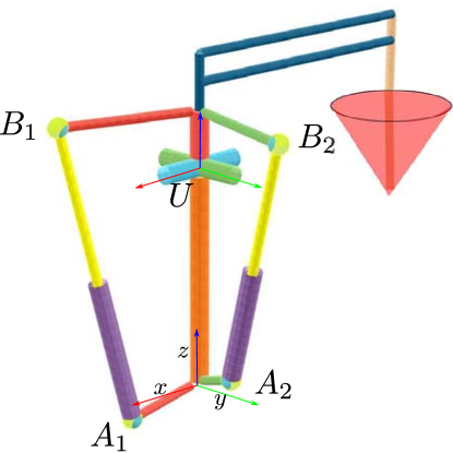
Figure 12: The parameters to be optimized in 2UPS-1U

The first joints in leg 1 and leg 2 with respect to the base can be given as:

$$A_{1}=\begin{bmatrix}a_{1}\cos\phi_{1}\\ a_{1}\sin\phi_{1}\\ h_{1}\end{bmatrix},\,A_{2}=\begin{bmatrix}a_{2}\cos\phi_{2}\\ a_{2}\sin\phi_{2}\\ h_{2}\end{bmatrix}$$

where, $a_{i}$ is the distance of the first joint of $i^{th}$ leg from the origin of the base frame and $\phi_{1}$ is the angle between the xy-projection of vector from the origin of the base frame to the joint and the x-axis. Similarly, $\phi_{2}$ is the angle between the xy-projection of vector from the origin of the base frame to the joint and the y-axis. The joints of each leg are at height $h_{1}$ and $h_{2}$ respectively. The universal joint (U) in the motion constraint generator leg is given as $[0,0,t]^{T}$ with respect to the base frame. The spherical joints in each leg are represented with respect to a frame with U as its origin and are given as:

$$B_{1}=\begin{bmatrix}b_{1}\cos\psi_{1}\\ b_{1}\sin\psi_{1}\\ h_{3}+t\end{bmatrix},\,B_{2}=\begin{bmatrix}b_{2}\cos\psi_{2}\\ b_{2}\sin\psi_{2}\\ h_{4}+t\end{bmatrix}$$

where, $b_{i}$ and $\psi_{i}$ are used to express the spherical joints in the legs and have similar interpretation as that of $a_{i}$ and $\phi_{i}$. The joints of each leg are at height $h_{3}+t$ and $h_{4}+t$ respectively.
Thus, the mechanism can be parameterized by 13 parameters after assuming that the motion constraint generator lies on the z-axis of the base. The 13 mechanism parameters to be optimized, as shown in figure 12 and detailed above are: $[a_{1},\phi_{1},h_{1},b_{1},\psi_{1},h_{2},a_{2},\phi_{2},h_{3},b_{2},\psi_{2},h_{4},t]$. The optimization parameters and the constraints along with their range are shown in Table 3.

Parameters	Value	Parameters	Value
optimization dimension	13	Range of $a_{i}$	[0.25, 1.5]
Range of $b_{i}$	[0.25, 2]	Range of $\phi_{i}$ and $\psi_{i}$	[-1.745, 1.745]
Range of $h_{i}$	[-0.1, 0.1]	Range of t	[1, 4]
Number of starts	200	Number of iterations	10 and 20
Objective choice	Workspace, GCI, VAF	Velocity amplification range	[0.3, 3]
Range of $b_{i}$	[0.25, 2]	Range of $\phi_{i}$ and $\psi_{i}$	[-1.745, 1.745]
Workspace (in roll and pitch)	circle of radius 1	stroke ratio	1.5
limits on spherical joints	$\pm\pi/6radians$	Collision constraint	considered

Table 3: The parameters set for the optimization of 2-dof RCM mechanism

The optimization of this mechanism was much longer than the previous example because of the increase in the optimization space, number of dof and the workspace considered. The regular dextrous workspace for the given mechanism is discussed in details in [43]. The results vary depending upon the objective choice as well as the rewarding strategy. We present the results obtained (Table 3) while optimizing for the GCI and rewarding a valid point in the workspace as 1 and 0 otherwise. The time required to evaluate one instance, i.e. one given set of parameters, was recorded along with the mean time for a single start, i.e. the complete operation till the algorithm stops to return the locally optimized parameters in 4. It was further analyzed to note the impact of different objective choices on the total optimization time. It was also noted that the fine search took a very long time compared to coarse searches, thus emphasizing the efficiency of the algorithm. The results are presented in Table 4 and computational time is recorded on the same system and is to be used for comparison only. Figure 13 presents the schematic plot for the mechanism optimized for maximum GCI along with the heatmap for the evaluation of GCI with the optimized parameters. Similarly, figure 14 illustrates the schematic as well as the heatmap of the quality related to the VAF for the corresponding optimized parameters. It is interesting to note from the schematics presented in both figures that the optimized parameters tend towards an architecture such that the actuated legs are $\frac{\pi}{2}$ radians apart and align along the axes of the universal joint present in the motion constraint generator. This observation also suggests that we can use human intuition and experience to reduce the dimension of the optimization space, resulting in faster optimization and designs that are easy to manufacture.

Parameters	GCI	VAF
Time for 1 coarse evaluation	14 seconds	18.3 seconds
Time for single coarse start	291 seconds	347.5 seconds
Time for one fine evaluation	50.5 seconds	51 seconds
Time for single fine start	1072 seconds	1077 seconds
Best point
$[a_{1},\phi_{1},h_{1},b_{1},\psi_{1},h_{2},a_{2},\phi_{2},$ $h_{3},b_{2},\psi_{2},h_{4},t]$ (refer figure 12)	[1.13, -1.02, -0.06, 1.47, -1.01, -0.05, 0.72, 0.44, -0.02, 1.52, 0.54, 0.02, 3.04]	[0.68, -0.25, 0.08, 1.03, 0.1, 0.04, 0.25, -1, 0.01, 1.1, -1.45, 0.17, 2.4]
Best actuator range	[2.54, 3.8]	[2, 3]
evaluation mean standard deviation	GCI 0.79 0.18	VAF 0.48 0.29
maximum evaluation configuration ($[\alpha,\beta])$	1 [0.39, 0.13]	0.99 [0, 0.43]
minimum evaluation configuration ($[\alpha,\beta])$	0.318 [0.86, 0.51]	-1.2 [-0.99, 0.14]

Table 4: The results for the optimization of 2-dof RCM mechanism

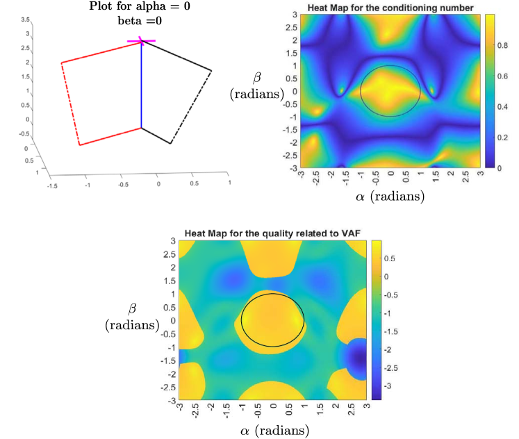
Figure 13: The schematic plot for the mechanism optimized for GCI and the heatmap for the evaluation. Calculation of GCI for this mechanism is discussed in [43]. The subfigure at the bottom is the heatmap for the VAF quality corresponding to the same parameters.

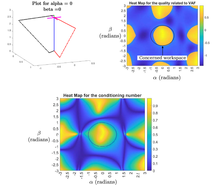
Figure 14: The schematic plot for the mechanism optimized for VAF and the heatmap for the evaluation. The subfigure at the bottom is the heatmap for the GCI corresponding to the same parameters.

5 Conclusions

In this paper, we present a novel optimization algorithm for parallel manipulators that is able to implement the joint limits and the collision of prismatic joints as constraints. The optimization methodology is also able to optimize the length of the actuator stroke, which enables the designer greater flexibility and clarity in the choice of the actuators. The algorithm uses geometrical traversing for optimization, which is very relevant for mechanism optimization. The algorithm implements a two-step search by combining a faster local search Nelder-Mead algorithm with initial simplexes spread over all the parameter space and then uses a finer search by using the locally optimized points in the step 1. The algorithm is general and can adapt to any non-redundant parallel mechanisms with prismatic as well as revolute joint. The paper presents two different mechanism optimization as an example to present the flexibility of the algorithm. The algorithm can be used in the systems that can propose different models based upon the requirements. In future works, the algorithm will be extended to multi-objective optimization to select the best architecture and corresponding design parameters of a robot for a given task.

References

- [1] J. P. Merlet, Parallel Robots, Springer, Netherlands, 2006.
- [2] Y. D. Patel, P. M. George, Parallel manipulators applications—a survey, Modern Mechanical Engineering 2 (3) (2012) 57–64.
- [3] A. Müller, D. Zlatanov (Eds.), Singular Configurations of Mechanisms and Manipulators, Vol. 589 of CISM International Centre for Mechanical Sciences, Springer International Publishing, Cham, Switzerland, 2019.
- [4] E. Gough, V, G. Whitehall, S, Universal tyre testing machine, in: Proceedings of International Congress FISITA, London, United Kingdom, 1962, pp. 117–137.
- [5] R. Clavel, Delta, a fast robot with parallel geometry, in: Proceedings of International Symposium on Industrial Robot, Lausanne, Switzerland, 1988, pp. 91–100.
- [6] B. Lee, C. Knabe, V. Orekhov, D. Hong, Design of a human-like range of motion hip joint for humanoid robots, in: Proceedings of the ASME 2014 International Design Engineering Technical Conferences & Computers and Information in Engineering Conference, Buffalo, New York, USA, 2014, pp. 8–18.
- [7] S. Lohmeier, T. Buschmann, H. Ulbrich, F. Pfeiffer, Modular joint design for performance enhanced humanoid robot LOLA, in: Proceedings 2006 IEEE International Conference on Robotics and Automation, IEEE, Orlando, FL, USA, 2006, pp. 88–93.
- [8] D. Kuehn, M. Schilling, T. Stark, M. Zenzes, F. Kirchner, System Design and Testing of the Hominid Robot Charlie: System Design and Testing of the Hominid Robot Charlie, Journal of Field Robotics 34 (4) (2017) 666–703.
- [9] S. Kumar, B. Bongardt, M. Simnofske, F. Kirchner, Design and kinematic analysis of the novel almost spherical parallel mechanism active ankle, Journal of Intelligent & Robotic Systems 94 (2) (2018) 303–325.
- [10] S. Kumar, H. Wöhrle, M. Trampler, M. Simnofske, H. Peters, M. Mallwitz, E. A. Kirchner, F. Kirchner, Modular design and decentralized control of the recupera exoskeleton for stroke rehabilitation, Applied Sciences 9 (4) (2019).
- [11] J. Arata, H. Kondo, M. Sakaguchi, H. Fujimoto, A haptic device delta-4: Kinematics and its analysis, in: Proceedings of World Haptics 2009 - Third Joint EuroHaptics conference and Symposium on Haptic Interfaces for Virtual Environment and Teleoperator Systems, Salt Lake City, UT, USA, 2009, pp. 452–457.
- [12] G. Michel, D. Salunkhe, D. Chablat, P. Bordure, A new RCM mechanism for an ear and facial surgical application, in: Proceedings of Advances in Service and Industrial Robotics, Springer International Publishing, Poitiers, France, 2020, pp. 408–418.
- [13] A. Dutta, D. H. Salunkhe, S. Kumar, A. D. Udai, S. V. Shah, Sensorless full body active compliance in a 6 DOF parallel manipulator, Robotics and Computer-Integrated Manufacturing 59 (2019) 278–290.
- [14] A. D. Udai, S. K. Saha, A. Dayal, Overlaid Orthogonal Force Oscillations for Robot Assisted Localization and Assembly, ISME Journal of Mechanics and Design 2 (1) (2018) 9–25.
- [15] S. Kumar, H. Wöhrle, J. de Gea Fernández, A. Müller, F. Kirchner, A survey on modularity and distributivity in series-parallel hybrid robots, Journal of Mechatronics 68 (2020).
- [16] J. Brinker, N. Funk, P. Ingenlath, Y. Takeda, B. Corves, Comparative Study of Serial-Parallel Delta Robots With Full Orientation Capabilities, IEEE Robotics and Automation Letters 2 (2) (2017) 920–926.
- [17] S. Caro, D. Chablat, R. Ur-Rehman, P. Wenger, Multiobjective design optimization of 3–PRR planar parallel manipulators, in: Proceedings of CIRP Design Conference, Nantes, France, 2010, pp. 373–383.
- [18] Z. Ma, A.-N. Poo, M. H. Ang, G.-S. Hong, H.-H. See, Design and control of an end-effector for industrial finishing applications, Robotics and Computer-Integrated Manufacturing 53 (2018) 240–253.
- [19] P. Wenger, D. Chablat, Kinematic analysis of a new parallel machine tool: the Orthoglide, in: Proceedings of Advances in Robot Kinematics, Slovenia, 2000, pp. 1–11.
- [20] C. Gosselin, J. Angeles, A global performance index for the kinematic optimization of robotic manipulators, Journal of Mechanical Design 113 (3) (1991) 220–226.
- [21] S. Chiu, Kinematic characterization of manipulators: an approach to defining optimality, in: Proceedings. 1988 IEEE International Conference on Robotics and Automation, Philadelphia, PA, USA, 1988, pp. 828–833.
- [22] D. Chablat, P. Wenger, F. Majou, The Optimal Design of Three Degree-of-Freedom Parallel Mechanisms for Machining Applications, in: In the Proceedings of 11th International Conference on Advanced Robotics, 2003, Coimbra, Portugal, 2003, pp. 1–6.
- [23] D. Chablat, P. Wenger, F. Majou, J.-P. Merlet, A novel method for the design of 2-dof parallel mechanisms for machining applications, International Journal of Robotics Research 23 (6) (2007) 615–624.
- [24] S. Kumar, A. Nayak, H. Peters, C. Schulz, A. Müller, F. Kirchner, Kinematic analysis of a novel parallel 2sprr+1u ankle mechanism in humanoid robot, in: Proceedings of Advances in Robot Kinematics, Bologna, Italy, 2018, pp. 431–439.
- [25] C. Germain, S. Caro, S. Briot, P. Wenger, Optimal design of the IRSBot-2 based on an optimized test trajectory, in: Proceedings of 37th Mechanisms and Robotics Conference, American Society of Mechanical Engineers, Portland, Oregon, USA, 2013, pp. 1–11.
- [26] M. H. Saadatzi, M. T. Masouleh, H. D. Taghirad, C. Gosselin, M. Teshnehlab, Multi-objective scale independent optimization of 3-RPR parallel mechanisms, in: Proceedings of 13th World Congress in Mechanism and Machine Science, Guanajuato, Mexico, 2011, pp. 1–11.
- [27] M. Gallant, R. Boudreau, The synthesis of planar parallel manipulators with prismatic joints for an optimal, singularity-free workspace, Journal of Robotic Systems 19 (1) (Jan. 2002).
- [28] S. Caro, D. Chablat, A. Goldsztejn, D. Ishii, C. Jermann, A branch and prune algorithm for the computation of generalized aspects of parallel robots, in: Principles and Practice of Constraint Programming, Berlin, Heidelberg, 2012, pp. 867–882.
- [29] S. Kucuk, A dexterity comparison for 3-DOF planar parallel manipulators with two kinematic chains using genetic algorithms, Mechatronics 19 (6) (2009) 868–877.
- [30] S. Ganesh, A. Koteswara Rao, B. Sarath kumar, Design optimization of a 3-DOF star triangle manipulator for machining applications, Materials Today: Proceedings 22 (12) (2020) 1845–1852.
- [31] A. Hassan, M. Abomoharam, Modeling and design optimization of a robot gripper mechanism, Robotics and Computer-Integrated Manufacturing 46 (2017) 94–103.
- [32] V. Muralidharan, A. Bose, K. Chatra, S. Bandyopadhyay, Methods for dimensional design of parallel manipulators for optimal dynamic performance over a given safe working zone, Mechanism and Machine Theory 147 (2020) 103721.
- [33] Z. Zhang, B. Chang, J. Zhao, Q. Yang, X. Liu, Design, optimization, and experiment on a bioinspired jumping robot with a six-bar leg mechanism based on jumping stability, Mathematical Problems in Engineering 2020 (2020) 1–23.
- [34] J.-A. Leal-Naranjo, J.-A. Soria-Alcaraz, C.-R. Torres-San Miguel, J.-C. Paredes-Rojas, A. Espinal, H. Rostro-González, Comparison of metaheuristic optimization algorithms for dimensional synthesis of a spherical parallel manipulator, Mechanism and Machine Theory 140 (2019) 586–600.
- [35] S. Ha, S. Coros, A. Alspach, J. Kim, K. Yamane, Computational co-optimization of design parameters and motion trajectories for robotic systems, The International Journal of Robotics Research 37 (13-14) (2018) 1521–1536.
- [36] N. Durand, J.-M. Alliot, A combined nelder-mead simplex and genetic algorithm, in: Proceedings of GECCO 1999, Genetic and Evolutionary Computation Conference, Orlando, FL, USA, 1999, pp. 1–7.
- [37] A. Koscianski, M. Luersen, Globalization and parallelization of Nelder-Mead and Powell optimization methods, in: Proceedings of Innovations and Advanced Techniques in Systems, Computing Sciences and Software Engineering, Dordrecht, Netherlands, 2008, pp. 93–98.
- [38] M. A. Luersen, R. Le Riche, Globalized Nelder–Mead method for engineering optimization, Computers & Structures 82 (23-26) (2004) 2251–2260.
- [39] P. Niegodajew, M. Marek, W. Elsner, Ł. Kowalczyk, Power plant optimisation—effective use of the Nelder-Mead approach, Processes 8 (3) (2020) 357.
- [40] R. A. Srivatsan, S. Bandyopadhyay, Determination of the safe working zone of a parallel manipulator, in: Proceedings of Computational Kinematics, Dordrecht, Netherlands, 2014, pp. 201–208.
- [41] K. H. Hunt, Review: don’t cross-thread the screw!, Journal of Robotic Systems 20 (7) (2003) 317–339.
- [42] D. Chablat, P. Wenger, Working modes and aspects in fully parallel manipulators, in: Proceedings of IEEE International Conference on Robotics and Automation, Vol. 3, Leuven, Belgium, 1998, pp. 1964–1969.
- [43] D. Chablat, G. Michel, P. Bordure, S. Venkateswaran, R. Jha, Workspace analysis in the design parameter space of a 2-DOF spherical parallel mechanism for a prescribed workspace: Application to the otologic surgery, Mechanism and Machine Theory 157 (Mar. 2021).
- [44] D. Chablat, P. Wenger, Moveability and Collision Analysis for Fully-Parallel Manipulators, in: Proceedings of RoManSy, Paris, France, 1998, pp. 1–8.
- [45] J.-P. Merlet, Trajectory verification of parallel manipulators in the workspace, The International Journal of Robotics Research 37 (13-14) (1994) 1–7.
- [46] J.-P. Merlet, Designing a parallel manipulator for a specific workspace, The International Journal of Robotics Research 16 (4) (1997) 545–556.
- [47] B. Danaei, N. Karbasizadeh, M. Tale Masouleh, A general approach on collision-free workspace determination via triangle-to-triangle intersection test, Robotics and Computer-Integrated Manufacturing 44 (2017) 230–241.
- [48] J. Pan, S. Chitta, D. Manocha, Fcl: A general purpose library for collision and proximity queries, in: 2012 IEEE International Conference on Robotics and Automation, 2012, pp. 3859–3866.
- [49] J. A. Nelder, R. Mead, A simplex method for function minimization, The Computer Journal 7 (4) (1965) 308–313.
- [50] J. C. Lagarias, J. A. Reeds, M. H. Wright, P. E. Wright, Convergence properties of the Nelder–Mead simplex method in low dimensions, SIAM Journal on Optimization 9 (1998) 7.
- [51] K. I. M. McKinnon, Convergence of the Nelder–Mead simplex method to a nonstationary point, SIAM Journal on Optimization 9 (1) (1998) 148–158.
- [52] P. C. Wang, T. E. Shoup, Parameter sensitivity study of the Nelder–Mead Simplex Method, Advances in Engineering Software 42 (7) (2011) 529–533.
- [53] D. Byatt, Convergent variants of the Nelder-Mead algorithm.pdf, Ph.D. thesis, University of Canterbury, England (2000).
- [54] S. Zapotecas Martínez, C. A. Coello Coello, A proposal to hybridize multi-objective evolutionary algorithms with non-gradient mathematical programming techniques, in: Proceedings of Parallel Problem Solving from Nature – PPSN X, Berlin, Heidelberg, 2008, pp. 837–846.
- [55] H. Niederreiter, Random number generation and quasi-monte carlo methods, in: Proceedings of CBMS-NSF regional conference series in applied mathematics, Vol. 63, Philadelphia, Pennsylvania, 1992, pp. 1 – 243.
- [56] K.-T. Fang, Y. Wang, Number-Theoretic Methods in Statistics, Chapman & Hall, London, 1994.
- [57] A. Alessandri, C. Cervellera, D. Macciò, M. Sanguineti, Optimization based on quasi-Monte Carlo sampling to design state estimators for nonlinear systems, Journal of Optimization 59 (2010) 963–984.
- [58] J. M. Hammersley, D. C. Handscomb, Monte Carlo Methods, Methuen, London, 1964.
- [59] A. Alessandri, C. Cervellera, M. Sanguineti, Design of asymptotic estimators: an approach based on neural networks and nonlinear programming, IEEE Trans. on Neural Networks 18 (1) (2007) 96–96.
- [60] I. M. Sobol’, The distribution of points in a cube and the approximate evaluation of integrals, Zh. Vychisl. Mat. i Mat. Fiz. 7 (1967) 784–802.
- [61] S. Bartsch, M. Manz, P. Kampmann, A. Dettmann, H. Hanff, M. Langosz, K. v. Szadkowski, J. Hilljegerdes, M. Simnofske, P. Kloss, M. Meder, F. Kirchner, Development and control of the multi-legged robot mantis, in: Proceedings of ISR 2016: International Symposium on Robotics, Munich, Germany, 2016, pp. 1–8.
- [62] J. Esser, S. Kumar, H. Peters, V. Bargsten, J. d. G. Fernandez, C. Mastalli, O. Stasse, F. Kirchner, Design, analysis and control of the series-parallel hybrid rh5 humanoid robot, in: 2020 IEEE-RAS 20th International Conference on Humanoid Robots (Humanoids), 2021, 2021, pp. 400–407.
- [63] S. Kumar, Modular and Analytical Methods for Solving Kinematics and Dynamics of Series-Parallel Hybrid Robots, Ph.D. thesis, University of Bremen, DFKI-RIC, Bremen, Germany (Sep. 2019).
- [64] C. Stoeffler, S. Kumar, H. Peters, O. Brüls, A. Müller, F. Kirchner, Conceptual design of a variable stiffness mechanism in a humanoid ankle using parallel redundant actuation, in: Proceedings of 18th International Conference on Humanoid Robots (Humanoids), Beijing, China, 2018, pp. 462–468.
- [65] M. Boukheddimi, S. Kumar, H. Peters, D. Mronga, R. Budhiraja, F. Kirchner, Introducing RH5 manus: A powerful humanoid upper body design for dynamic movements, in: 2022 IEEE International Conference on Robotics and Automation (ICRA), 2022.